Figure 5: Rain intensity in the control simulation at 05:00 UTC (corresponding with the time the S For flare is positioned over Australia). major rainfall increases occurred over land in Queensland and Indonesia (Figure 3b). Other flare simulations showed a similar behaviour for their respective regions (not shown).
is only slightly greater than its control simulation. This suggests that the presence of land is important for triggering convection and enhancing rainfall due to a superflare.
In order to observe the longer-term effects of the S For flare on a particular region, average daily rainfall was calculated over the boxes in Figure 2. Figure 4 shows time series of total daily rainfall for each box for the control and flare simulations as well as the corresponding means. The means of daily rain for superflare simulations are greater than the control simulations, therefore a greater amount of rain fell in the weeks following a superflare. Unlike the continental simulations, rainfall in the Pacific simulation
5. Discussion and Conclusion The S For flare is much more powerful than the others due to its higher energy and shorter duration. Its short duration also means that the affected area is much smaller. The difference between June and January SST is due to the maximum insolation being located in the North West Pacific Ocean in June and Australia in January. The o Aql and 5 Ser flares are five and three days in duration
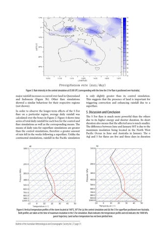
Figure 6: Vertical temperature profiles of the storm located at 140째E, 30째S for (a) the control simulation and (b) the S For superflare positioned over Australia. Both profiles are taken at the time of maximum insolation in the S For simulation. Black indicates the temperature profile and red indicates the 1000 hPa parcel trajectory. Land surface temperature has not been plotted here. Bulletin of the Australian Meteorological and Oceanographic Society Vol. 27 page 31