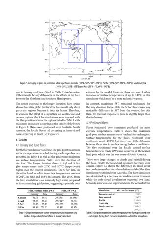
Figure 2: Averaging regions for positioned S For superflares. Australia (10°N–50°S, 90°E–170°E), Pacific (10°N–50°S, 180°E–260°E), South America (10°N–50°S, 255°E–355°E) and Asia (55°N–5°S, 60°E–140°E). run in January and June (listed in Table 2) to determine if there would be any differences in the effects of the flare between the Northern and Southern Hemispheres.
estimate by the model. However, there are several other instances of surface temperatures of up to 140°C in this simulation which may be a more realistic response.
The region exposed to the longer duration flares spans almost the entire globe, but the S For flare would only affect particular regions because it lasts six hours. Therefore, to examine the effect of a superflare on continental and oceanic regions, the S For simulations were repeated with the flare positioned over the regions listed in Table 3 with maximum insolation occurring at the centre of the boxes in Figure 2. Flares were positioned over Australia, South America, the Pacific Ocean (all occurring in January) and Asia (occurring in June) (see Figure 2).
In contrast, maximum SSTs remained unchanged for the long duration flares. Only the S For flare causes any noticeable difference in SST from the control. For this flare, the thermal response in June is slightly larger than that in January.
4. Results 4.1 January and June flares For the flares in January and June, the grid point maximum surface temperatures reached during each superflare are presented in Table 4 as well as the grid point maximum sea surface temperatures (SSTs) over the duration of the flare. The longer duration flares o Aql and 5 Ser give temperatures only 2.7°C and 5.7°C (respectively) higher than the control simulations. The S For flare, on the other hand, resulted in surface temperature maxima of 201°C in June and 188°C in January. The 201°C from the June simulation is an unusually high value compared to its surrounding grid points, suggesting a possible over Max. surface temp. (°C) January June Control 55.75 59.45 o Aql 58.35 58.45 5 Ser 59.45 65.15 S For 188.49 201.05
Max. SST(°C) January June 29.4554 30.4985 29.5149 30.503 29.5385 30.568 30.491 30.974
Table 4: Gridpoint maximum surface temperature and maximum sea surface temperature for each flare in January and June. Bulletin of the Australian Meteorological and Oceanographic Society Vol. 27 page 29
4.2 Positioned flares Flares positioned over continents produced the most extreme temperatures. Table 5 shows the maximum grid point surface temperatures reached for each region. Surface temperatures for the flares positioned over continents reach 202°C but there was little difference between them due to surface energy balance conditions. The flare positioned over the Pacific caused surface temperatures to reach 109°C and occurred at the nearest land point which was the west coast of South America. There were large changes to clouds and rainfall during the flares. Firstly, the total cloud coverage decreased over oceans. Figure 3a shows the difference in cloud cover fraction between the control simulation and the S For flare simulation positioned over Australia. The flare simulation was dominated by a decrease in cloudiness over the ocean while the only cloud development occurred over land. Secondly, rain was also suppressed over the ocean but the Simulation January control June control Pacific Australia South America Asia
Max. surface temp.!(°C) 55.65 59.25 110.65 203.75 203.45 203.25
Table 5: Grid point maximum surface temperature for flares positioned over each region during the S Fornacis simulations and control simulations.