D (sec)
∆W(B) (Wm-2)
1.00×1028
1030
220.33
27
2400
19.83
28
600
386.00
26
2100
2.26
S For
31
2.00×10
1120
466585.30
BD + 10
3.00×1027
2940
24.28
o Aql
9.00×1029
432000
49.57
5 Ser
30
259200
642.63
28
3420
487.05
Star Gmb 1830 k Ceti MT Tau Pi Uma
UU CrB
Energy (J)
2.00×10 1.00×10 2.00×10
7.00×10 7.00×10
Table 1: A list of superflares from Schaefer et al. (2000), including S Fornacis, with their total energies, durations D and the maximum anomalous radiation flux at the top of the atmosphere ∆W(B).
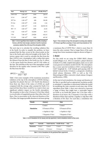
Figure 1: Time evolution of top of the atmosphere incoming solar radiation of S Fornacis superflares assuming 3.5 hours and 6 hours duration at 1 AU from the Sun.
The next step is to calculate the resulting radiation flux at the Earth. In order to simplify the problem, we have assumed that the flare occurs at the closest point on the Sun to the Earth and is directed straight at the Earth. The inverse square rule is used to calculate the flux from the flare (∆W(t)) over a hemisphere with a radius that spans the distance from the flare to the Earth (e.g. Eq. 5), where r is the mean Earth-Sun distance and R is the radius of the Sun. The total flux at the top of the atmosphere would therefore be the regular solar constant (1365 Wm-2) plus the flux from the flare.
a maximum flux of 22978 Wm-2, which is more than 16 times the solar constant. That is, longer flares of the same energy have lower maximum output as shown in Figure 1.
!! ! !
! ! !! ! ! !
(5)
!
Table 1 lists some examples of the maximum anomalous radiation at the top of the atmosphere (∆W(B)) during a superflare for planets that are 1 AU (Earth-Sun distance) from their star. Most of the values of ∆W(B) are small compared with the average solar constant for Earth. It is expected that these flares would be too weak to have any significant radiative impact on the Earth’s atmosphere. The exception to this is the S Fornacis (S For) flare which is several orders of magnitude greater than other observed flares. Due to uncertainty in the observed duration of the S For flare, the longest possible duration is six hours giving Month
Simulation
3. Model For this study we are using the CSIRO Mk3L climate model (Phipps et al., 2011) to simulate a planet identical to Earth. It is a fully coupled atmosphere, land, sea ice and ocean general circulation model (GCM). The atmosphere has a coarse spectral resolution of R21 corresponding to 5.625° longitude by ~3.18° latitude grid spacing with 18 hybrid vertical levels. It features a prognostic stratiform cloud scheme (Rotstayn, 1997) as well as the U.K. Meteorological Office convective cloud scheme (Gregory and Rowntree, 1990). At the start of each simulation, the energy and duration of the flare is specified and an appropriate insolation profile is calculated. A superflare is represented within the model by modifying the solar constant at each time step. Of the superflares from Table 1, three were selected to represent a range of flares that might have a noticeable impact on Earth or an Earth-like planet: the S For flare with a duration of six hours, the 5 Serpentis (5 Ser) flare with a duration of three days and the o Aquilae (o Aql) flare with a duration of five days. For each flare, a simulation was
January
June
Control
Control
S Fornacis (S For)
S Fornacis (S For)
o Aquilae (o Aql)
o Aquilae (o Aql)
5 Serpentis (5 Ser)
5 Serpentis (5 Ser)
Table 2: A list of simulations for the January and July experiment. Control simulations involve no flare event. Region
Australia
South America
Pacific Ocean
Asia
Simulation
Control
Control
Control
Control
S Fornacis
S Fornacis
S Fornacis
S Fornacis
Table 3: A list of simulations for the positioned flares experiment. Bulletin of the Australian Meteorological and Oceanographic Society Vol. 27 page 28