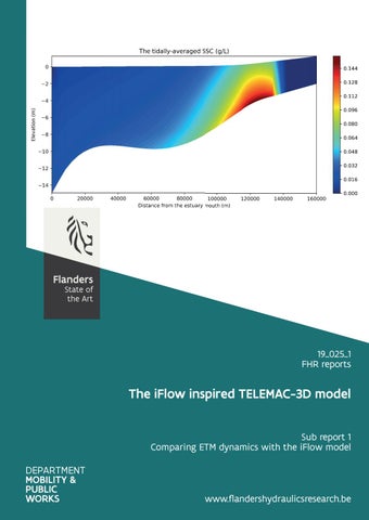
19_025_1 FHR reports
The iFlow inspired TELEMAC-3D model Sub report 1 Comparing ETM dynamics with the iFlow model
www.flandershydraulicsresearch.be
The iFlow inspired TELEMAC-3D model Sub report 1 – Comparing ETM dynamics with the iFlow model
Bi, Q.; Kaptein, S. J.; Schramkowski, G.; Smolders, S.; Mostaert, F.
Cover figure © The Government of Flanders, Department of Mobility and Public Works, Flanders Hydraulics Research Legal notice Flanders Hydraulics Research is of the opinion that the information and positions in this report are substantiated by the available data and knowledge at the time of writing. The positions taken in this report are those of Flanders Hydraulics Research and do not reflect necessarily the opinion of the Government of Flanders or any of its institutions. Flanders Hydraulics Research nor any person or company acting on behalf of Flanders Hydraulics Research is responsible for any loss or damage arising from the use of the information in this report. Copyright and citation © The Government of Flanders, Department of Mobility and Public Works, Flanders Hydraulics Research 2020 D/2020/3241/180 This publication should be cited as follows: Bi, Q.; Kaptein, S. J.; Schramkowski, G.; Smolders, S.; Mostaert, F. (2020). The iFlow inspired TELEMAC-3D model: Sub report 1 – Comparing ETM dynamics with the iFlow model. Version 3.0. FHR Reports, 19_025_1. Flanders Hydraulics Research: Antwerp Reproduction of and reference to this publication is authorised provided the source is acknowledged correctly. Document identification Customer: Keywords (3-5): Knowledge domains
Waterbouwkundig Laboratorium Ref.: WL2020R19_025_1 Numerical modelling, iFlow, Telemac, ETM Hydrodynamics > Tides > Numerical modelling Hydrodynamics > Current velocities and patterns > Numerical modelling Hydrodynamics > Water levels > Numerical modelling Sediment > Cohensive > Numerical modelling Sediment > Sediment balance > Numerical modelling
Text (p.): Confidentiality:
39 ܈No
Author(s):
Bi, Q.; Kaptein, S. J.; Schramkowski, G.
Appendices (p.): ܈Available online
9
Control Name Reviser(s):
Project leader:
Smolders, S.
Kaptein, S. J.
Signature Getekend door: Sven Smolders (Signature) Getekend op: 2020-09-16 09:19:38 +01:00 Reden: Ik keur dit document goed
Getekend door: Steven Kaptein (Signature) Getekend op: 2020-09-15 08:32:08 +01:00 Reden: Ik keur dit document goed
Approval Head of Division:
F-WL-PP10-2 Version 7 Valid as from 3/01/2017
Mostaert, F.
Getekend door: Frank Mostaert (Signature) Getekend op: 2020-09-14 15:06:14 +01:00 Reden: Ik keur dit document goed
The iFlow inspired TELEMAC-3D model - Sub report 1 – Comparing ETM dynamics with the iFlow model
Abstract This report is the first part of the comparison study of the two different modelling approaches, idealised modelling using iFlow, and idealised modelling using TELEMAC-3D. The TELEMAC computational domain used in this study is inspired by the iFlow model of the Scheldt estuary from Brouwer et al., 2018. In the iFlow study, the model is used for studying the time evolution of estuarine turbidity maximum (ETM) in the Scheldt. Both computational efficiency and the well-presented physical processes in this iFlow model makes capturing ETM zones possible. However, reproducing ETM dynamics still faces challenges in the TELEMAC-3D or other large-scale complex models. This study tries to find out the necessary model set-ups required for capturing an ETM in a TELEMAC-3D model, with the inspirations from the iFlow model.
Final version
WL2020R19_025_1
III
F-WL-PP10-2 Version 7 Valid as from 3/01/2017
The iFlow inspired TELEMAC-3D model - Sub report 1 – Comparing ETM dynamics with the iFlow model
Contents Abstract ............................................................................................................................................................ III Contents ............................................................................................................................................................ V List of tables...................................................................................................................................................... VI List of figures ................................................................................................................................................... VII 1
Introduction ............................................................................................................................................... 1
2
TELEMAC-3D – GAIA .................................................................................................................................. 2
3
2.1
The governing equations ................................................................................................................... 2
2.2
Turbulence models ............................................................................................................................ 2
2.3
Bottom boundary condition .............................................................................................................. 3
The iFlow-inspired Scheldt model ............................................................................................................. 4 3.1
3.1.1
Schematization of the Scheldt ................................................................................................... 5
3.1.2
The range of physical parameters ............................................................................................. 6
3.1.3
The boundary forcing ................................................................................................................ 6
3.2
5
The TELEMAC-3D model .................................................................................................................... 6
3.2.1
The Schematized unstructured mesh ........................................................................................ 7
3.2.2
Bottom friction law .................................................................................................................... 7
3.2.3
Sediment diameter and the settling velocity ............................................................................ 8
3.2.4
Lateral boundary conditions ...................................................................................................... 8
3.2.5
Bottom boundary condition .................................................................................................... 12
3.2.6
The initial concentration field ................................................................................................. 12
3.3 4
The inspirations from the iFlow model ............................................................................................. 5
Model comparison........................................................................................................................... 14
Investigating ETM with the TELEMAC-3D model..................................................................................... 18 4.1
The reference model ....................................................................................................................... 18
4.2
The influence of the initial concentration ....................................................................................... 25
4.3
The influence of the settling velocity .............................................................................................. 27
4.4
The influence of upstream discharge .............................................................................................. 28
4.5
The influence of the grid resolution ................................................................................................ 33
Conclusion ............................................................................................................................................... 38
Reference ........................................................................................................................................................ 39 Appendix I. Steering file of Telemac-3D (hydrodynamics) .............................................................................. A1 Appendix II. Steering file of GAIA (sediment transport) .................................................................................. A8
Final version
WL2020R19_025_1
V
The iFlow inspired TELEMAC-3D model - Sub report 1 – Comparing ETM dynamics with the iFlow model
List of tables Table 1 – iFlow Model parameter values representative for the Scheldt Estuary ............................................ 6 Table 2 – Model set-up of iFlow and TELEMAC-3D model .............................................................................. 14 Table 3 – List of the runs with the equilibrium boundary condition ............................................................... 18
VI
WL2020R19_025_1
Final version
The iFlow inspired TELEMAC-3D model - Sub report 1 – Comparing ETM dynamics with the iFlow model
List of figures Figure 1 – The Scheldt Estuary .......................................................................................................................... 4 Figure 2 – The measured and fitted geometry of the Scheldt Estuary ............................................................. 5 Figure 3 – The schematized domain of the Scheldt Estuary (Brouwer et al., 2018) used in the iFlow model .. 5 Figure 4 – The unstructured Telemac grid of the schematized Scheldt estuary ............................................... 7 Figure 5 – The bottom elevation of the unstructured Telemac grid ................................................................. 7 Figure 6 – Comparison of the concentration profiles given by the equilibrium boundary condition............. 11 Figure 7 – The vertical concentration profiles at the seaward boundary in 6 tidal cycles .............................. 11 Figure 8 – The tidally-averaged SSC from the iFlow model results with Q=60m3/s ........................................ 12 Figure 9 – The iFlow results (tidally-averaged surface SSC at 150 days) and the fitted data.......................... 13 Figure 10 – Comparison of M2 amplitude between iFlow and Telemac models ............................................ 15 Figure 11 – Comparison of M2 phase between iFlow and Telemac models ................................................... 15 Figure 12 – Comparison of M4 amplitude between iFlow and Telemac models ............................................ 15 Figure 13 – Comparison of M4 phase between iFlow and Telemac models ................................................... 16 Figure 14 – Comparison of the sediment concentration along the thalweg................................................... 16 Figure 15 – Comparison of the sediment transport rate along the thalweg................................................... 17 Figure 16 – The equilibrium boundary conditions at the seaward boundary ................................................. 19 Figure 17 – The initial concentration field derived from the iFlow result ....................................................... 19 Figure 18 – Tidally averaged SSC along the thalweg (EBC_ws=2.8mms_Q=20m³s_initSSC) after 294 days... 20 Figure 19 – Cumulative bed evolution (m) at the end of the simulation (EBC_ws=2.8mms_Q=20m³s_initSSC) ......................................................................................................................................................................... 20 Figure 20 – Time evolution of the residual advective sediment transport (EBC_ws=2.8mms_Q=20m³s_initSSC) ............................................................................................................. 21 Figure 21 – Time evolution of the sediment mass in the domain (EBC_ws=2.8mms_Q=20m³s_initSSC) ...... 21 Figure 22 – Time evolution of the residual reconstructed total sediment transport (EBC_ws=2.8mms_Q=20m³s_initSSC) ............................................................................................................. 22 Figure 23 – Reconstructed tidally averaged sediment transport and the changes of mass in bed (EBC_ws=2.8mms_Q=20m³s_initSSC), ............................................................................................................ 22 Figure 24 – Comparison of the residual sediment transport (EBC_ws=2.8mms_Q=20m³s_initSSC).............. 23 Figure 25 – Comparison of sediment flux at the seaward boundary (EBC_ws=2.8mms_Q=20m³s_initSSC) . 24 Figure 26 – Comparison of sediment flux at 10 km (EBC_ws=2.8mms_Q=20m³s_initSSC) ............................ 24 Figure 27 – Tidally averaged SSC along the thalweg (EBC_ws=2.8mms_Q=20m³s) after 294 days................ 25 Figure 28 – Time evolution of the residual advective sediment transport (EBC_ws=2.8mms_Q=20m³s_initSSC) ............................................................................................................. 25 Figure 29 – Time evolution of the sediment mass in the domain (EBC_ws=2.8mms_Q=20m³s) ................... 26 Final version
WL2020R19_025_1
VII
The iFlow inspired TELEMAC-3D model - Sub report 1 – Comparing ETM dynamics with the iFlow model
Figure 30 – Time evolution of the residual reconstructed total sediment transport (EBC_ws=2.8mms_Q=20m³s) .......................................................................................................................... 26 Figure 31 – Tidally averaged SSC along the thalweg (EBC_ws=2.0mms_Q=20m3s_initSSC) after 294 days .. 27 Figure 32 – Time evolution of the residual reconstructed total sediment transport (EBC_ws=2.0mms_Q=20m3s_initSSC) ............................................................................................................ 28 Figure 33 – Time evolution of the sediment mass in the domain (EBC_ws=2.0mms_Q=20m3s_initSSC) ..... 28 Figure 34 – Tidally averaged SSC along the thalweg (EBC_ws=2.8mms_Q=80m3s_initSSC) .......................... 29 Figure 35 – Comparison of the tidally-averaged depth average SSC along thalweg....................................... 29 Figure 36 – Cumulative bed evolution (m) at the end of the simulation (EBC_ws=2.8mms_Q=80m3s_initSSC) ......................................................................................................................................................................... 30 Figure 37 – Time evolution of the residual advective sediment transport (EBC_ws=2.8mms_Q=80m3s_initSSC) ............................................................................................................ 30 Figure 38 – Time evolution of the sediment mass in the domain (EBC_ws=2.8mms_Q=80m3s_initSSC) ..... 31 Figure 39 – Time evolution of the residual reconstructed total sediment transport (EBC_ws=2.8mms_Q=80m3s_initSSC) ............................................................................................................ 31 Figure 40 – Comparison of the residual sediment transport (EBC_ws=2.8mms_Q=20m3s_initSSC and EBC_ws=2.8mms_Q=80m3s_initSSC), ............................................................................................................. 32 Figure 41 – Reconstructed tidally averaged sediment transport and the changes of mass in bed (EBC_ws=2.8mms_Q=20m3s_initSSC and EBC_ws=2.8mms_Q=80m3s_initSSC),.......................................... 32 Figure 42 – Comparison of the grid size used in the model ............................................................................ 33 Figure 43 – Comparison of water level M2 and M4 amplitudes with different grids ..................................... 34 Figure 44 – Comparison of water level M2 and M4 phases with different grids ............................................ 34 Figure 45 – Comparison of horizontal depth averaged velocity M2 and M4 amplitudes with different grids 35 Figure 46 – Comparison of horizontal depth averaged velocity M2 and M4 phases with different grids ...... 35 Figure 47 – Comparison of the residual sediment transport with different grid sizes ................................... 36 Figure 48 – Time evolution of the residual reconstructed total sediment transport (EBC_ws=2.8mms_Q=80m3s_initSSC_fine_grid) ............................................................................................ 36 Figure 49 – Tidally averaged SSC along the thalweg (EBC_ws=2.8mms_Q=80m3s_initSSC_fine_grid) ......... 37 Figure 50 – Time evolution of the sediment mass in the domain (EBC_ws=2.8mms_Q=80m3s_initSSC_fine_grid) ............................................................................................ 37
VIII
WL2020R19_025_1
Final version
The iFlow inspired TELEMAC-3D model - Sub report 1 – Comparing ETM dynamics with the iFlow model
1 Introduction The iFlow model represents the an idealised, 'exploration' type of modelling approach while the TELEMAC-3D model represents the complex, three-dimensional 'case-study' type of modelling approach. Both the iFlow model and TELEMAC-3D model have their advantages and disadvantages. On the one hand, iFlow is renowned for its computational efficiency and capability of revealing many transport mechanisms in idealised modelling of hydrodynamics and sediment transport. However, it can only deal with simplified or schematized domains since it uses width-averaged governing equations. Additionally, the resolution of these equations in iFlow is based on the perturbation technique, which linearizes the equations but limits the reproduction of the high-order physical processes. On the other hand, TELEMAC-3D solves the Navier-Stokes equation in 3D domain, thus, it overcomes iFlow's disadvantages but at the expense of much higher computational cost. For example, in this study the average computational time for the iFlow model is within 1s on a laptop with one processor, while for Telemac-3D model one-year simulation is about 8 hours on a cluster with 36 processors. This feature makes the 'exploration' study, e.g. investigating the dynamics of estuarine turbidity maximum (ETM) zones in the Scheldt with a TELEMAC-3D model difficult, since it often requires a long simulation period for the system to reach the equilibrium. In addition, the calibration of a 3D sediment transport model requires searching for an optimal set of parameters in a high-dimensional parameter space. Therefore, not many studies were able to achieve this goal successfully using such complex numerical models. In the study of Brouwer et. al, 2018, the iFlow modelling approach is employed. An idealised Scheldt model was built using iFlow. The model was then used for studying the time evolution of ETM and its equilibrium state in the Scheldt. Both computational efficiency and the well-presented physical processes in this iFlow model made capturing ETM zones possible. Subsequently, this study tries to find out the necessary model set-ups required for capturing ETM in a TELEMAC-3D model, with the inspirations from the iFlow model.
Final version
WL2020R19_025_1
1
The iFlow inspired TELEMAC-3D model - Sub report 1 – Comparing ETM dynamics with the iFlow model
2 TELEMAC-3D – GAIA 2.1 The governing equations TELEMAC-3D is a module in the openTelemac suite for modelling 3D hydrodynamics. The hydrodynamics in TELEMAC-3D is modelled with 3D incompressible Reynolds-averaged Navier-Stokes equations. The Navier–Stokes equations for incompressible flows consist of two equations: the continuity equation and the momentum equation. Assuming that fluid density is constant, and applying the Boussinesq eddy viscosity approximation to the Reynolds stress term, the mass and momentum conservation equations read: ∇ ∙ đ??Žđ??Ž = 0
1 ∂đ??Žđ??Ž + (đ??Žđ??Ž â‹… ∇)đ??Žđ??Ž = − ∇đ?‘?đ?‘? + ∇ â‹… [(ν + ν đ?‘‡đ?‘‡ )∇đ??Žđ??Ž] + đ?? đ?? + đ??…đ??… Ď âˆ‚đ?‘Ąđ?‘Ą
(1)
(2)
where đ??Žđ??Ž is the Reynolds-averaged mean velocity field, đ?‘Ąđ?‘Ą is the time, đ?œŒđ?œŒ is the fluid density, đ?‘?đ?‘? is the mean pressure, đ?œˆđ?œˆ is the kinematic viscosity of the fluid, đ?œˆđ?œˆđ?‘‡đ?‘‡ is the turbulence eddy viscosity, đ?? đ?? is the gravitational force and đ??…đ??… is the other external forces, e.g. Coriolis force and centrifugal force. The suspended sediment transport can be solved by the following transport equation using the available numerical solvers in TELEMAC-3D: ∂đ?‘?đ?‘? + (đ??Žđ??Ž â‹… ∇)đ?‘?đ?‘? = ∇ â‹… (đ??ˇđ??ˇđ?‘‡đ?‘‡ ∇đ?‘?đ?‘? + đ??°đ??°đ??Źđ??Ź đ?‘?đ?‘? ) ∂đ?‘Ąđ?‘Ą
(3)
where đ?‘?đ?‘? is the sediment concentration, đ??ˇđ??ˇđ?‘‡đ?‘‡ is the turbulent diffusion coefficient, đ??°đ??°đ??Źđ??Ź is the settling velocity vector pointing downward. However, in order to provide the necessary bottom boundary conditions for the transport equation, the erosion and deposition fluxes have to be computed. This is done in GAIA, which is a sediment transport module in the openTelemac suite. Therefore, in order to have a complete 3D sediment transport model, TELEMAC-3D has to be coupled with GAIA. In many industrial and environmental flows, the density of the carrying phase is not a constant but varies as a function of the temperature, salinity and/or sediment concentration. The buoyancy effects due to the density gradient thus should be included in the governing equations in order to model the stratification properly. The varying density could be included in the Eq. (1) and Eq. (2). But there is also an alternative way that enables the treatment of buoyancy effect by means of the gravity term if the change of density ∆đ?œŒđ?œŒâ „đ?œŒđ?œŒ < 0.1. Based on this assumption, an extra term representing the buoyancy force can be derived and added into the momentum equation. The details can be found in the TELEMAC-3D theory guide.
2.2 Turbulence models To solve the above equations, The turbulence eddy viscosity ν đ?‘‡đ?‘‡ has to be closed with a turbulence model. In large-scale modelling, the water depth is often not of the same order of magnitude as the horizontal dimensions of the domain. Hence, the domain discretization usually leads to a much coarser mesh resolution in horizontal, and relatively finer mesh resolution in vertical, meaning that the turbulence eddies that represented in horizontal and in vertical are of different scales. Hence, it is necessary for the users to choose the turbulence models wisely depending on the application. Several turbulence models are available in the TELEMAC-3D. The most commonly used ones are đ?‘˜đ?‘˜ − Ďľ model, the Smagorinski model and the mixing-length model. It is also possible for the users to define constant eddy viscosity for horizontal and vertical, respectively. In this study the k-Ďľ model is adopted in all the simulations.
2
WL2020R19_025_1
Final version
The iFlow inspired TELEMAC-3D model - Sub report 1 – Comparing ETM dynamics with the iFlow model
The two-equation đ?‘˜đ?‘˜ − Ďľ model consists of two transport equations for the turbulence kinetic energy and its dissipation rate, It defines the eddy viscosity as: ν đ?‘‡đ?‘‡ = đ??śđ??śÎź
đ?‘˜đ?‘˜ 2 Ďľ
The two transport equations for the turbulence kinetic energy and its dissipation rate reads: ν đ?‘‡đ?‘‡ ∂đ?‘˜đ?‘˜ + đ??Žđ??Ž â‹… ∇đ?‘˜đ?‘˜ = đ?‘ƒđ?‘ƒ + ∇ â‹… ��ν + ďż˝ ∇đ?‘˜đ?‘˜ďż˝ − Ďľ + đ??şđ??ş Ďƒđ?‘˜đ?‘˜ ∂đ?‘Ąđ?‘Ą
ν đ?‘‡đ?‘‡ âˆ‚Ďľ Ďľ Ďľ2 ( ) + đ??Žđ??Ž â‹… âˆ‡Ďľ = đ??śđ??ś1Ďľ đ?‘ƒđ?‘ƒ + đ??śđ??ś3Ďľ đ??şđ??ş − đ??śđ??ś2Ďľ + ∇ â‹… ��ν + ďż˝ âˆ‡Ďľďż˝ ∂đ?‘Ąđ?‘Ą đ?‘˜đ?‘˜ ĎƒĎľ đ?‘˜đ?‘˜
(4) (5)
(6)
where đ??Žđ??Ž is the velocity vector, đ?‘˜đ?‘˜ is the turbulence kinetic energy, Ďľ is the dissipation rate at which turbulence kinetic energy is converted into thermal internal energy, đ?‘ƒđ?‘ƒ is the production term and đ??şđ??ş is the buoyancy term. đ??śđ??śÎź , đ??śđ??ś1Ďľ , đ??śđ??ś2Ďľ and đ??śđ??ś3Ďľ are model constants.
2.3 Bottom boundary condition
Both of the iFlow and TELEMAC-3D models assume the hydraulic rough condition at bottom (TELEMAC-3D can also deal with hydraulic smooth flow), and both of them need to compute shear velocity as the boundary condition at bottom when solving the governing equations. However, the major differences between iFlow and TELEMAC-3D resides in the treatment at the bottom boundary. On the one hand, TELEMAC-3D adopts the quadratic law for computing the shear velocity at bottom: ν
∂đ??Žđ??Žđ?›•đ?›• 1 = đ??śđ??śđ?‘“đ?‘“ đ??Žđ??Žđ?›•đ?›• đ??Žđ??Žđ?›•đ?›• , 2 ∂đ?‘›đ?‘›
(7)
∂đ??Žđ??Žđ?›•đ?›• = đ?‘†đ?‘†đ?‘“đ?‘“ đ??Žđ??Žđ?›•đ?›• , ∂đ?‘›đ?‘›
(8)
WL2020R19_025_1
3
where đ??śđ??śđ?‘“đ?‘“ is a dimensionless friction coefficient (drag coefficient), and đ?‘˘đ?‘˘Ď„ is the near-bottom velocity (on the lowest mesh layer) at a certain distance from the wall. On the other hand, iFlow assumes a similar partial slip condition, but with a linear formulation of the velocity dependence of the stresses at the bottom: ν
where ���� is a dimensionless friction coefficient in iFlow. For consistency with the iFlow model, the linear friction law Eq. (8) was implemented in TELEMAC-3D, as an additional option for the keyword LAW OF BOTTOM FRICTION.
Final version
The iFlow inspired TELEMAC-3D model - Sub report 1 – Comparing ETM dynamics with the iFlow model
3 The iFlow-inspired Scheldt model By far, capturing the dynamics of the estuarine turbidity maximum (ETM) in the Scheldt with a large-scale complex model still remains the most challenging. Not many numerical models succeed in reproducing stable ETM zones within their modelled domain. Usually it requires a long simulation period for the model to reach an equilibrium state, which is computational expensive, particularly for a 3D sediment transport model. Figure 1 – The Scheldt Estuary
One of the tricks often being used in the sediment transport models is placing a bed layer on the bottom as part of the initial conditions. This layer consists of the same sediment material used in the simulation, and can be a few centimetres thick. It provides the source for erosion and is available from the beginning. Due to the fact that, the third ETM zone also corresponds more or less to the region where the largest tidal energy occurs (Chen et al., 2005), it is possible to form a high concentrated zone due to high erosion rates and local re-suspension. However, this mechanism does not correspond to the main reason for the ETM zone formed here and it cannot sustain the ETM zone for a long period. As a consequence, the bed layer is continuously eroded and eventually the sediment supply runs out. The high concentration zone, therefore, gradually fades away. Most of the material is transported downstream and exported out of the modelled domain. In contrast, the iFlow model for the Scheldt is able to reproduce ETM zones in an schematized domain. The iFlow model is based on a totally different philosophy. When solving the governing equations for the hydrodynamics and sediment transport, instead of looking for the solutions for each time step, iFlow uses the perturbation technique to decompose the unknown variables, resulting in different orders of contributions, and then solve them in the frequency domain. Nevertheless, iFlow and TELEMAC-3D share the same governing equations. Therefore, they could, in principal, produce similar results when the application fulfils assumptions that hold in both models. However, one of the advantages of the iFlow model is the computational efficiency. For example, a one-year TELEMAC3D simulation (6744 nodes/per plane Ă— 6 planes, timestep 10s) would take about 6 days running on one processor. With the same computing power, the similar iFlow model needs less than 2 seconds to complete. Although the iFlow model is a two-dimensional vertical model, it lacks some information along the y-axis. For example, it does not take into account the inter-tidal areas explicitly. Despite these shortcomings, it is still useful when the study focus on the horizontal variations. Since the iFlow model is fast and able to capture the ETM zones in Scheldt, one of the goals in this study is to combine the efficiency of iFlow model and the 3D modelling capability of TELEMAC, to investigate how to capture the ETM zones in large-scale numerical models and which modelling parameters are important.
4
WL2020R19_025_1
Final version
The iFlow inspired TELEMAC-3D model - Sub report 1 – Comparing ETM dynamics with the iFlow model
3.1 The inspirations from the iFlow model The studies from Dijkstra et al. (2017) and Brouwer et al. (2018) provide many insights in terms of modelling the ETM dynamics in Scheldt using iFlow. Since both of them could reproduce ETMs in their models, in this report, we try to follow their approach in three aspects: • • •
the schematization of the domain, the possible range of parameters, and the boundary conditions.
With these input parameters, we will set-up a TELEMAC-3D model for simulating hydrodynamics and sediment transport in the Scheldt. 3.1.1
Schematization of the Scheldt
The geometry of the Scheldt Estuary has been schematized by a funnel-shaped domain in the studies of Dijkstra et al. (2017) and Brouwer et al. (2018), based on observations. As shown in Figure 2 and Figure 3, the schematized geometry is derived by fitting an exponential function of a ratio of two polynomials against observed width along the Scheldt estuary. Similarly, the bottom in the schematized domain is obtained by fitting a smooth function to the measured cross-sectionally averaged depth along the estuary. Figure 2 – The measured and fitted geometry of the Scheldt Estuary (Dijkstra et al., 2017)
Figure 3 – The schematized domain of the Scheldt Estuary (Brouwer et al., 2018) used in the iFlow model
Final version
WL2020R19_025_1
5
The iFlow inspired TELEMAC-3D model - Sub report 1 – Comparing ETM dynamics with the iFlow model
The schematized domain starts at Vlissingen the estuary mouth, and ends all the way up to the Gentbrugge where tidal locks were installed. The total length is 160km. The width is about 13.3km at the mouth and about 90m at the upstream boundary. 3.1.2
The range of physical parameters
Based on this schematized domain of the Scheldt Estuary, an idealised width-averaged process-based iFlow model has been created. Table 1 gives an overview of the important physical parameters used in the iFlow model. Table 1 – iFlow Model parameter values representative for the Scheldt Estuary (Brouwer et al., 2018)
For simplicity, turbulence is modelled with constant eddy viscosity. A linear roughness law (eq. 8) is used at the bottom as the partial slip boundary, and the roughness parameter is kept constant as well. For the sediment transport, a constant vertical diffusivity and a much larger horizontal eddy diffusivity are used to implicitly account for the additional diffusion caused by salinity, which is not included in the model. The sediment grain size remains fixed and uniform, as well as the settling velocity. The erosion parameter is a calibration parameter and it is chosen from 1.0 × 10⁻⁵ to 1.0 × 10⁻⁴. 3.1.3
The boundary forcing
The iFlow model has two open boundaries. At the seaward, a tidal forcing consisting of M2 and M4 harmonic constituents is prescribed. The two major tidal signals are superposed with a relative phase difference in order to generate tidal asymmetry that is similar to the observations. A sediment concentration is also imposed at the seaward boundary(see Table 1). The upstream boundary has a constant fresh water inflow, with no sediment input from the river.
3.2 The TELEMAC-3D model A TELEMAC-3D model, including hydrodynamics and sediment transport (by coupling with GAIA), was created using the same schematized geometry and bathymetry as described in §3.1.1. The model settings are also kept as close as possible to those in the iFlow model as they can be.
6
WL2020R19_025_1
Final version
The iFlow inspired TELEMAC-3D model - Sub report 1 – Comparing ETM dynamics with the iFlow model
3.2.1
The Schematized unstructured mesh
TELEMAC uses unstructured triangular mesh for the computation, meaning that the grid size can vary spatially. The advantage is that it can capture the exact geometry of the domain while remaining computational efficient by using coarser grid in the regions that do not require high accuracy. To make the exact the same computational domain, the geometry and bathymetry data is taken the same as in the schematized Scheldt iFlow model (Dijkstra et al., 2017 and Brouwer et al., 2018). Figure 4 – The unstructured Telemac grid of the schematized Scheldt estuary
0 km
160 km Figure 5 – The bottom elevation of the unstructured Telemac grid
0 km
160 km
The fitted geometry of the schematized Scheldt Estuary from iFlow Scheldt model is imported into Gmsh to create the unstructured mesh for TELEMAC-3D model. In order to have a lightweight mesh that allows the model running efficiently, the grid density is defined as a function of the width along the estuary. This results in a mesh that is symmetric about the x-axis. There are always four elements distributed along the y-axis at each kilometre, and those elements are aligned with the streamlines from downstream until the very upstream. The final mesh size ranges from about 4000m in the estuary mouth to about 30m in the upstream boundary (Figure 4). Then, the fitted bathymetry from the iFlow model is mapped to the TELEMAC-3D grid (Figure 5). The construction of the 3D mesh in Telemac is done by stacking multiple 2D planes together. In this study, six horizontal planes are distributed evenly in vertical (sigma layers). The total distance between the surface plan and the bottom plan equals to the water depth and it can change at each time step, but the ratios between them are always constant. 3.2.2
Bottom friction law
One of the major differences between TELEMAC-3D and iFlow is the bottom boundary condition. As stated before in §2.3, they both assume a hydraulic rough condition at bottom. But TELEMAC-3D employs a quadratic law for computing the shear velocity, while iFlow uses a linear friction law. For better comparison, the same linear friction law has been carefully implemented in the TELEMAC-3D model. To be more specific,
Final version
WL2020R19_025_1
7
The iFlow inspired TELEMAC-3D model - Sub report 1 – Comparing ETM dynamics with the iFlow model
the iFlow's linear friction law has been added to the source file telemac3d.dico as the 6th option for the TELEMAC-3D keyword LAW OF BOTTOM FRICTION. Then in the source file tfond.f, the corresponding part for computing the shear velocity is added: ELSEIF (KFROT.EQ.6) THEN DO N=1,NPOIN UETCAR(N) = SQRT(U3D(N)**2+V3D(N)**2)*RUGOF0 ENDDO ELSE
The roughness coefficient is read from the keyword FRICTION COEFFICIENT FOR THE BOTTOM and assigned to the variable RUGOF0. The bottom velocity is calculated as the norm of the velocity vector on the bottom plane. 3.2.3
Sediment diameter and the settling velocity
Settling velocity of the sediment is an important parameter since it is related to many physical processes, e.g. transport, erosion and deposition. The settling velocity in the TELEMAC-3D model is kept uniform and constant in time. It is calculated based on the sediment diameter from a so-called Stokes Law if the settling velocity is not given in the model set-ups: đ?‘”đ?‘”đ?‘‘đ?‘‘ 2 ďż˝Ď đ?‘?đ?‘? − Ď đ?‘šđ?‘š ďż˝ (9) đ?‘¤đ?‘¤đ?‘ đ?‘ = 18Îź in which, đ?‘¤đ?‘¤đ?‘ đ?‘ is the settling velocity, đ?‘”đ?‘” is the acceleration of gravity, đ?‘‘đ?‘‘ is the particle diameter, Ď đ?‘?đ?‘? is the particle density, Ď đ?‘šđ?‘š is the medium density and Îź is the dynamic viscosity of medium.
In this study, only one class of cohesive sediment is considered. The sediment diameter is chosen from the range 60 - 80 micrometre based on the measured mean particle diameter in the Scheldt (Fettweis et al., 2003; van Kessel et al., 2011; Dam and Bliek, 2013). The density is set to 1800 kg/m3, implicitly including the flocculation. Hence, the settling velocity ranges from about 1.5 mm/s to 2.8 mm/s. 3.2.4
Lateral boundary conditions
The TELEMAC-3D model also has two open boundaries, one downstream, at the landward side and the other upstream, at the seaward side. Seaward boundary conditions The seaward boundary has prescribed water levels. The same tidal forcing from the iFlow model consisting of M2 and M4 signals is imposed at the seaward boundary for both inflow and outflow: đ?œ đ?œ đ?‘ đ?‘ đ?‘ đ?‘ đ?‘ đ?‘ = đ??´đ??´đ?‘šđ?‘š2 đ?‘?đ?‘?đ?‘?đ?‘?đ?‘?đ?‘?(đ?œ”đ?œ”đ?‘šđ?‘š2 đ?‘Ąđ?‘Ą + đ?œ™đ?œ™đ?‘šđ?‘š2 ) + đ??´đ??´đ?‘šđ?‘š4 đ?‘?đ?‘?đ?‘?đ?‘?đ?‘?đ?‘?(đ?œ”đ?œ”đ?‘šđ?‘š4 đ?‘Ąđ?‘Ą + đ?œ™đ?œ™đ?‘šđ?‘š4 )
(10)
where đ?œ đ?œ đ?‘ đ?‘ đ?‘ đ?‘ đ?‘ đ?‘ is the water level prescribed at the seaward boundary, đ?‘Ąđ?‘Ą is time, đ??´đ??´đ?‘šđ?‘š2 and đ??´đ??´đ?‘šđ?‘š4 are the amplitude of M2 tide and M4 tide, respectively, đ?œ”đ?œ”đ?‘šđ?‘š2 and đ?œ”đ?œ”đ?‘šđ?‘š4 are the angular frequency of the M2 and M4 tides, respectively, and đ?œ™đ?œ™đ?‘šđ?‘š2 and đ?œ™đ?œ™đ?‘šđ?‘š4 are the phases of M2 and M4 tides, respectively. The water level prescribed at the seaward boundary is computed in the source file sl3.f):
!
APPLY THE HARMONIC CONSTITUENTS PI = ACOS(-1.D0) A_M2 = 1.77D0 A_M4 = 0.14D0 PHI_M2 = 0.D0 PHI_M4 = -1.3D0*PI/180.D0 FREQ_M2 = 2.D0*PI/(3600.D0*12.42) FREQ_M4 = 2.D0*FREQ_M2 SL3=A_M2*COS(FREQ_M2*TIME+PHI_M2)+A_M4*COS(FREQ_M4*TIME+PHI_M4)
8
WL2020R19_025_1
Final version
The iFlow inspired TELEMAC-3D model - Sub report 1 – Comparing ETM dynamics with the iFlow model
The sediment concentration is also imposed at the seaward boundary. By default, the imposed concentration is only prescribed during the inflow. During the outflow, the boundary type for the sediment is changed from Dirichlet to Neumann, meaning that the values at the boundary nodes are determined by the nearby concentration gradient. This treatment of the boundary is called Thatcher-Harleman boundary condition. However, instead of using the default option, we use another type of boundary condition called the equilibrium boundary for the sediment transport. The sediment concentration is prescribed during both inflow and outflow, unlike the Thatcher-Harleman boundary condition. Moreover, the concentration is not constant anymore. Instead, it is time-dependent and calculated based on the equilibrium condition at the bottom, under which the erosion rate is assumed to be the same as the deposition rate, as described hereafter. If we consider 1DV steady flow, the sediment transport is described as: đ?œ•đ?œ•đ?œ•đ?œ• đ?œ•đ?œ•đ?œ•đ?œ• đ?œ•đ?œ• + ďż˝đ??ˇđ??ˇđ?‘‡đ?‘‡ + đ?‘¤đ?‘¤đ?‘ đ?‘ đ??śđ??śďż˝ = 0 đ?œ•đ?œ•đ?œ•đ?œ• đ?œ•đ?œ•đ?œ•đ?œ• đ?œ•đ?œ•đ?œ•đ?œ•
(11)
in which, đ??śđ??ś is the sediment concentration, đ??ˇđ??ˇđ?‘‡đ?‘‡ is the eddy diffusivity of the sediment particles, đ?‘¤đ?‘¤đ?‘ đ?‘ is the settling velocity of the sediment, đ?‘Ąđ?‘Ą is time and đ?‘§đ?‘§ is the vertical coordinate.
Applying the equilibrium conditions at the sediment bottom by assuming constant and uniform settling velocity and eddy viscosity, one could end up with an exponential concentration profile that can be prescribed at the seaward boundary during both inflow and outflow: đ??śđ??ś (đ?‘§đ?‘§) = đ?‘?đ?‘?đ?‘?đ?‘? ∙ đ?‘’đ?‘’ −đ?‘¤đ?‘¤đ?‘ đ?‘ đ?‘§đ?‘§/đ??ˇđ??ˇđ?‘‡đ?‘‡
(12)
đ?‘?đ?‘?đ?‘?đ?‘? = đ??¸đ??¸/đ?‘¤đ?‘¤đ?‘ đ?‘
(13)
đ??¸đ??¸ = đ?‘€đ?‘€đ?œ?đ?œ?đ?‘?đ?‘?
(14)
đ?‘§đ?‘§ đ?œˆđ?œˆđ?‘Ąđ?‘Ą = đ?‘˘đ?‘˘âˆ— ∙ đ?œ…đ?œ…đ?œ…đ?œ… ∙ ďż˝1 − ďż˝ â„Ž
(15)
in which đ?‘?đ?‘?đ?‘?đ?‘? is the near-bed concentration, and it can be calculated from: The erosion rate is scale with the bed shear stress only, as it is computed in the iFlow:
Similarly, instead of a constant value over the entire water column, if we assume the eddy viscosity has a parabolic profile according to the mixing-length theory,
the concertation profile will become a so-call Rouse profile: đ??śđ??ś (đ?‘§đ?‘§) = đ?‘?đ?‘?đ?‘?đ?‘? ∙ ďż˝
đ?‘§đ?‘§ đ??ťđ??ť − đ?‘§đ?‘§đ?‘?đ?‘? −đ?‘¤đ?‘¤đ?‘ đ?‘ /đ?œ…đ?œ…đ?‘˘đ?‘˘âˆ— ďż˝ đ??ťđ??ť − đ?‘§đ?‘§ đ?‘§đ?‘§đ?‘?đ?‘?
(16)
in which, đ?œˆđ?œˆđ?‘Ąđ?‘Ą is the eddy viscosity, đ??ťđ??ť is the water depth, đ?‘§đ?‘§đ?‘?đ?‘? is the reference level for the near-bed concentration, đ?œ…đ?œ… is the von Karman constant and đ?‘˘đ?‘˘âˆ— is the shear velocity. In this study, the concentration at the seaward boundary is computed from eq. (13), eq. (14) and eq. (16).
The TELEMAC-3D source files user_bord3d.f and cvdf3d.f are modified to incorporate the equilibrium boundary conditions for sediment transport. The implementation consists of two parts. The first part is the modifications in cvdf3d.f to enforce the Dirichlet type boundary condition for sediment concentration during inflow and outflow. This is done by commenting the section from line 355 to line 369: ! ! ! !!
IF(NPTFR3.GT.0.AND.NFRLIQ.GT.0.AND..NOT.VELOCITY) THEN DO IPTFR=1,NPTFR3 IF(LIFBOL%I(IPTFR).EQ.KENT) THEN EXITS ARE TREATED AS FREE BOUNDARIES Final version
WL2020R19_025_1
9
The iFlow inspired TELEMAC-3D model - Sub report 1 – Comparing ETM dynamics with the iFlow model
! ! ! ! ! ! ! ! ! ! !
IP=NBOR3%I(IPTFR) IF(FLUEXTPAR%R(IP).GT.0.D0) LIFBOL%I(IPTFR)=KSORT ELSEIF(LIFBOL%I(IPTFR).EQ.KSORT) THEN IP=NBOR3%I(IPTFR) IF(FLUEXTPAR%R(IP).LT.0.D0) THEN LIFBOL%I(IPTFR)=KENT FBORL%R(IPTFR)=FN%R(IP) ENDIF ENDIF ENDDO ENDIF
The second part of the modifications are done in the file user_bord3d.f for computing the concentration at the boundary nodes. The reference level is chosen at 5 cm above the bed. Both upstream and seaward boundary are treated here, but for ensuring the zero sediment input from the river, the erosion rate at the upstream boundary is set to zero, hence the concentration over the whole water column is kept zero. ! !
!
! !
BEGIN OF EQUILIBRIUM BC FOR SEDIMENT ITRAC = 1 M1 = 0.D0 M2 = 6.0D-5 TAU_C = 0.1D0 ZB = 0.05D0 DO K=1,NPTFR2 IF(BOUNDARY_COLOUR%I(K).EQ.1350) J1=K ! middle point of upstream bc IF(BOUNDARY_COLOUR%I(K).EQ.2701) J2=K ! middle point of dowstream bc ENDDO
ROUSE PROFILE DO K=1,NPTFR2 DO NP=1,NPLAN IBORD = (NP-1)*NPTFR2+K IF(LITABL%ADR(ITRAC)%P%I(IBORD).EQ.KENT) THEN IF(BOUNDARY_COLOUR%I(K).GE.1348 .AND. & BOUNDARY_COLOUR%I(K).LE.1352) THEN J=J1 M=M1 ELSE J=J2 M=M2 ENDIF ZSURF=Z(NBOR3%I((NP-1)*NPTFR2+J)) ZZ=MAX(ZB,ZSURF-Z(NBOR3%I(J))) HH=Z(NBOR3%I((NPLAN-1)*NPTFR2+J))-Z(NBOR3%I(J)) WSS=WCHU%ADR(ITRAC)%P%R(IBORD) USTAR=DSQRT(UETCAR%R(NBOR3%I(J))) E=MAX(0.D0,M*(UETCAR%R(NBOR3%I(J))*1.D3)) TABORL%ADR(ITRAC)%P%R(IBORD)=E/WSS* & (ZZ/(HH-ZZ)*(HH-ZB)/ZB)**(-WSS/(0.4D0*USTAR)) ENDIF ENDDO ENDDO ! END OF EQUILIBRIUM BC FOR SEDIMENT
Figure 6 shows the different concentration profiles given by eq. (12) and eq. (16), respectively. Although the near-bed concentration is the same, the Rouse profile gives larger concentration gradient near the bottom 10
WL2020R19_025_1
Final version
The iFlow inspired TELEMAC-3D model - Sub report 1 – Comparing ETM dynamics with the iFlow model
and lower concentration in the water column, due to the more realistic parabolic profile for eddy viscosity (Mofjeld 1988). Hence, in this study, the Rouse profile is used in the equilibrium boundary conditions for sediment. The time evolution of the concentration profiles at the seaward boundary is illustrated in Figure 7. Figure 6 – Comparison of the concentration profiles given by the equilibrium boundary condition
Figure 7 – The vertical concentration profiles at the seaward boundary in 6 tidal cycles
Final version
WL2020R19_025_1
11
The iFlow inspired TELEMAC-3D model - Sub report 1 – Comparing ETM dynamics with the iFlow model
River boundary conditions The upstream boundary is a constant river discharge. In the model tests, the discharge is set to 20 m3/s for the low discharge scenario and 80 m3/s for the high discharge scenario. Furthermore, it is assumed that there is no sediment input from the river, the same assumption as in the iFlow model. 3.2.5
Bottom boundary condition
The following equation is used as the boundary condition near the bed for the suspended sediment transport equation (taken at a reference height đ?‘§đ?‘§đ?‘?đ?‘? above the bed): −đ??ˇđ??ˇđ?‘Łđ?‘Ł
đ?œ•đ?œ•đ?œ•đ?œ• − đ?‘¤đ?‘¤đ?‘ đ?‘ đ??śđ??ś = (đ??¸đ??¸ − đ??ˇđ??ˇ)đ?‘§đ?‘§đ?‘?đ?‘? đ?œ•đ?œ•đ?œ•đ?œ•
(17)
đ?œ•đ?œ•đ?œ•đ?œ• ďż˝ = đ??¸đ??¸ đ?œ•đ?œ•đ?œ•đ?œ• đ?‘§đ?‘§đ?‘?đ?‘?
(18)
where đ??ˇđ??ˇđ?‘Łđ?‘Ł is the vertical eddy diffusivity, đ??śđ??ś is the sediment concentration, đ?‘§đ?‘§ is the vertical coordinate, đ?‘¤đ?‘¤đ?‘ đ?‘ is the settling velocity, đ??¸đ??¸ is the erosion flux and the deposition flux đ??ˇđ??ˇ = đ?‘¤đ?‘¤đ?‘ đ?‘ đ??śđ??ś. Then the bottom boundary for the transport equation becomes: −đ??ˇđ??ˇđ?‘Łđ?‘Ł
This is a Neumann type boundary and it states that the diffusive flux is balanced by the erosion flux at the bottom. In TELEMAC-3D, the erosion flux has slightly different form from the one used in the iFlow model: đ?œ?đ?œ?đ?‘?đ?‘? đ??¸đ??¸ = max ďż˝0, đ?‘€đ?‘€ ďż˝ − 1�� đ?œ?đ?œ?đ?‘?đ?‘?
(19)
where, đ??¸đ??¸ is the erosion rate, đ?‘€đ?‘€ is the erosion parameter, đ?œ?đ?œ?đ?‘?đ?‘? is the bed shear stress and đ?œ?đ?œ?đ?‘?đ?‘? is the critical shear stress for erosion. In iFlow model, the erosion rate is simply scaled with the bed shear stress, as expressed in eq. (14). 3.2.6
The initial concentration field
One of the issues for sediment transport modelling is the model initialization. The iFlow model does not require initial conditions since the governing equations are solved in the frequency domain, thus only the boundary conditions are needed. On the other hand, the initialization of the 3D large-scale sediment transport model usually takes months to reach an equilibrium state. The main reason is that, the temporal and spatial varying concentration field adds more complexity to the system and slows down the evolution of the system towards the equilibrium. Figure 8 – The tidally-averaged SSC from the iFlow model results with Q=60m3/s (Brouwer et al., 2018)
12
WL2020R19_025_1
Final version
The iFlow inspired TELEMAC-3D model - Sub report 1 – Comparing ETM dynamics with the iFlow model
To accelerate the initialization of the model, the concentration filed computed from the iFlow model is used to initialize the concentration field in the TELEMAC-3D model. The tidally-averaged surface SSC from Brouwer et al. (2018) is adopted for making the initial concentration field for TELEMAC-3D model (Figure 8). Figure 9 – The iFlow results (tidally-averaged surface SSC at 150 days) and the fitted data
The tidally-averaged surface SSC after150 days is taken every 5 km along the estuary, then these data points are fitted with a polynomial of 20 degree. When imposing the initial concentration to the TELEMAC-3D model, the vertical concentration profiles are needed. For simplicity, the constant vertical profile is given, which means the values along vertical will be the same. Thus, the fitted polynomial is then multiplied by 2 for better approximating the depth-averaged SSC, and then the values are duplicated on each plane. In this way, the Initial mass will be well approximated. For imposing an initial concentration field to TELEMAC-3D model, the source file user_condi3d_trac.f is modified: DO I = 1,NPOIN2 DO IPLAN = 1,NPLAN J = (IPLAN-1)*NPOIN2 + I TA%ADR(1)%P%R(J) =(2.35800340405229D-94*X(I)**20.D0& 3.97026818398674D-88*X(I)**19.D0+ & 3.07898028631538D-82*X(I)**18.D0& 1.45963993753503D-76*X(I)**17.D0+ & 4.73416591751121D-71*X(I)**16.D0& 1.11404646362240D-65*X(I)**15.D0+ & 1.96835923762031D-60*X(I)**14.D0& 2.66593265227820D-55*X(I)**13.D0+ & 2.80156209981808D-50*X(I)**12.D0& 2.29793521819673D-45*X(I)**11.D0+ & 1.47259103829669D-40*X(I)**10.D0& 7.34674630481110D-36*X(I)**9.D0+ & 2.83028981870196D-31*X(I)**8.D0& 8.30657501557918D-27*X(I)**7.D0+ & 1.81962783285209D-22*X(I)**6.D0& 2.88569041869754D-18*X(I)**5.D0+ & 3.16159286915740D-14*X(I)**4.D0& 2.21783488576179D-10*X(I)**3.D0+ & 8.80050009327383D-07*X(I)**2.D0& 0.00204144732657153D0*X(I)**1.D0+ & 25.4929214733874D0)*2.D0/1.D3 ENDDO ENDDO
Final version
WL2020R19_025_1
13
The iFlow inspired TELEMAC-3D model - Sub report 1 – Comparing ETM dynamics with the iFlow model
3.3 Model comparison The iFlow-inspired TELEMAC-3D is compared with the iFlow model for checking if the two can match each other’s results.. The harmonic analysis is only performed with the water level along the thalweg points from both model results. The model set-up of both iFlow model and TELEMAC-3D model are listed in Table 2. The M2 and M4 components are shown in Figure 10 - Figure 13. Table 2 – Model set-up of iFlow and TELEMAC-3D model
Model settings
iFlow model
TELEMAC-3D model
Upstream discharge
80 m3/s
80 m3/s
Seaward BC - M2 amp., phase
1.77 m, 0.0 degree
1.77 m, 0.0 degree
Seaward BC – M4 amp., phase
0.14 m, -1.3 degree
0.14 m, -1.3 degree
Bottom roughness
Spatial varying coefficients
0.0048
Turbulence model
Spatial varying coefficients
k-epsilon model
Initial conditions
Not required
constant surface elevation, zero velocity, SSC field obtained from the iFlow model result
It is worth mentioning that iFlow model uses bottom roughness and eddy viscosity as calibration parameters for getting better agreement with the Telemac-3D model results. Hence, spatial varying coefficients are used in the iFlow model. Despite the differences in the parameters, in general, the M2 amplitudes obtained from the TELEMAC-3D model has a good agreement with the result from the iFlow model, with deviations in the region from 140 km to 160 km. The maximum difference is about 0.1 m at 152 km. The M2 phases also show a good agreement between the two models from 0 km to 140 km. Again, they start to deviate from each other in the region from 140 km to 160 km, and the difference becomes larger towards the upstream. The M4 amplitudes do not match very well between the TELEMAC-3D model and iFlow model. The maximum deviation is about 0.2 m at 132 km. But instead of giving lower values, this time the iFlow model predicts higher amplitude. It is known that some physics are not well caught in the iFlow model. In particular, iFlow is linearized based on the assumption that the tidal amplitude is small with respect to the water-depth, which is not satisfied in the upper part of the estuary. This feature could result in deviations in the M4 tide, hence this is no surprise here. The M4 phases obtained from the iFlow model and TELEMAC-3D model shows better agreement than the M4 amplitudes, with deviations only in the upstream from 142 km to 160 km.
14
WL2020R19_025_1
Final version
The iFlow inspired TELEMAC-3D model - Sub report 1 – Comparing ETM dynamics with the iFlow model Figure 10 – Comparison of M2 amplitude between iFlow and Telemac models
Figure 11 – Comparison of M2 phase between iFlow and Telemac models
Figure 12 – Comparison of M4 amplitude between iFlow and Telemac models
Final version
WL2020R19_025_1
15
The iFlow inspired TELEMAC-3D model - Sub report 1 – Comparing ETM dynamics with the iFlow model Figure 13 – Comparison of M4 phase between iFlow and Telemac models
The sediment distribution in the model is compared. In this comparison, multiple upstream discharges are tested in order to show the system reactions. It can be seen in Figure 14 that both models can capture the ETM with different discharges. The concentration is lower in the TELEMAC-3D model. This could be due to a slightly different erosion law used in the TELEMAC-3D, but more tests need to be done to investigate the exact reason. However, the ETM in both models react to the upstream discharge in a similar way. When the discharge becomes higher, the horizontal SSC profile tends to shift towards downstream, i.e. SSC decreases from 138 km to 160 km whereas it increases from about 40km to 138 km. But again, the shift is larger in the iFlow model and the location of ETM peak does not move in the TELEMAC-3D model. Figure 14 – Comparison of the sediment concentration along the thalweg (left: iFlow model, right: TELEMAC-3D model)
The total sediment transport rate along the thalweg also shows a similarity between the two models. After reaching the equilibrium, they both show a constant transport rate from the seaward boundary to a certain point in the upstream (Figure 15). The iFlow result has a different transport rate unit from the TELEMAC-3D result, but after conversion they show the same magnitude. For example, with the 80 m3/s upstream discharge, TELEMAC-3D model reaches about 1.3 kg/s constant transport rate in the downstream area. Then the transport rate decreases to zero because there is no input from the landward boundary. Both models show the similar behaviour when upstream discharge is increased. In this case, the transport rate becomes smaller, and the turning point shifts downstream.
16
WL2020R19_025_1
Final version
The iFlow inspired TELEMAC-3D model - Sub report 1 – Comparing ETM dynamics with the iFlow model Figure 15 – Comparison of the sediment transport rate along the thalweg (left: iFlow model, right: TELEMAC-3D model)
The comparisons of the hydrodynamics and the ETM dynamics between the two models suggest, although they belong to two different modelling approaches, and some of the model settings and parameters are different, they are able to produce similar results. Moreover, the similar system reactions to the upstream boundary conditions indicate both models could reproduce the similar physical processes.
Final version
WL2020R19_025_1
17
The iFlow inspired TELEMAC-3D model - Sub report 1 – Comparing ETM dynamics with the iFlow model
4 Investigating ETM with the TELEMAC-3D model For revealing the influence of different factors/conditions on the simulation results, e.g. initial conditions, settling velocity, discharge, etc., a reference model was created. Three additional runs, with slight different model settings were made for comparison with the reference. The list of the runs used in this section is shown in Table 3. Table 3 – List of the runs with the equilibrium boundary condition
Run ID
Settling velocity
Discharge
Initial concentration
EBC_ws=2.8mms_Q=20m3s_init.SSC (reference)
2.8 mm/s
20 m3/s
Derived from the iFlow model
EBC_ws=2.8mms_Q=20m3s
2.8 mm/s
20 m3/s
zero
EBC_ws=2.0mms_Q=20m3s_init.SSC
2.0 mm/s
20 m3/s
Derived from the iFlow model
EBC_ws=2.8mms_Q=80m3s_init.SSC
2.8 mm/s
80 m3/s
Derived from the iFlow model
In the four model runs listed in Table 3, two kinds of initial concentrations are tested, the initial concentration field derived from the iFlow model result, and zero initial concentration imposed in the whole domain; two settling velocities are compared, the first one is about 2.0 mm/s corresponding to the particle with diameter of 70 micrometre and density of 1800 kg/m3, the second one is about 2.8 mm/s corresponding to the particle with diameter of 80 micrometre and density of 1800 kg/m3; two river discharges are used at the upstream boundary, the low discharge scenario with 20 m3/s and the high discharge scenario with 80 m3/s; moreover, the influence of grid resolution is also investigated. The simulation period is 365 days and only the results near the end of the simulation are used for further analysis.
4.1 The reference model The reference model (EBC_ws=2.8mms_Q=20m3s_init.SSC) has the same M2 and M4 tidal forcing imposed at the seaward boundary as in the iFlow model. The forcing consist of a M2 signal with amplitude of 1.77 m and phase of 0 degree, and a M4 signal with amplitude of 0.14 m and phase of -1.3 degree. The water level is computed by the supposition of the M2 and M4 signals according to the Eq. (10) in §3.2.4, and then prescribed at the boundary. The equilibrium boundary condition for the sediment transport is implemented in the model. As explained in §3.2.4, the concentration imposed at the seaward boundary is computed according to the Eq.(16). Given the M2 and M4 forcing at the boundary, under the equilibrium condition between erosion and deposition at the bottom, the concentration profile can be computed as a function of the time, the reference bed level, the local shear velocity and the settling velocity, and imposed during both inflow and outflow (Figure 16).
18
WL2020R19_025_1
Final version
The iFlow inspired TELEMAC-3D model - Sub report 1 – Comparing ETM dynamics with the iFlow model Figure 16 – The equilibrium boundary conditions at the seaward boundary
Figure 17 – The initial concentration field derived from the iFlow result
The model starts with an initial concentration field derived from iFlow model results as described in §3.2.6. As shown in Figure 17, the concentration stays constant vertically, with variations only in horizontal. The thickness of bed layer in the model is initially set to zero. The settling velocity in the reference model is set to about 2.8 mm/s, which corresponds to the sediment particle with diameter of 80 micrometre and density of 1800 kg/m3, according to the Stokes law of settling velocity described in Eq. (9). The upstream discharge is 20 m3/s, resembling the low discharge scenario. As seen in Figure 18, the ETM zone is found in the reference model EBC_ws=2.8mms_Q=20m3s_initSSC with the low discharge scenario (20 m3/s). The ETM is formed in the region starting from about 105 km to 135 km. Moreover, a bed layer is formed a bit further upstream at about 150 km (Figure 19). As seen in the figures Figure 21, Figure 22 and Figure 23, the equilibrium is reached in the one-year simulation.
Final version
WL2020R19_025_1
19
The iFlow inspired TELEMAC-3D model - Sub report 1 – Comparing ETM dynamics with the iFlow model Figure 18 – Tidally averaged SSC along the thalweg (EBC_ws=2.8mms_Q=20m³s_initSSC) after 294 days
Figure 19 – Cumulative bed evolution (m) at the end of the simulation (EBC_ws=2.8mms_Q=20m³s_initSSC)
The time evolution of the net advective sediment transport in a tidal cycle is computed according to the Eq. (20) and plotted in Figure 20. đ?‘†đ?‘†đ?‘Žđ?‘Žđ?‘Žđ?‘Žđ?‘Žđ?‘Ž (đ?‘Ľđ?‘Ľ ) = ďż˝ �� đ?‘˘đ?‘˘(đ?‘Ľđ?‘Ľ, đ?‘Śđ?‘Ś, đ?‘§đ?‘§, đ?‘Ąđ?‘Ą) ∙ đ?‘?đ?‘? (đ?‘Ľđ?‘Ľ, đ?‘Śđ?‘Ś, đ?‘§đ?‘§, đ?‘Ąđ?‘Ą) đ?‘‘đ?‘‘đ?‘‘đ?‘‘đ?‘‘đ?‘‘đ?‘‘đ?‘‘ďż˝ đ?‘‘đ?‘‘đ?‘‘đ?‘‘ đ?‘‡đ?‘‡
đ?‘…đ?‘…
(20)
where, đ?‘†đ?‘†đ?‘Žđ?‘Žđ?‘Žđ?‘Žđ?‘Žđ?‘Ž is the net advective sediment transport in a tidal cycle, đ?‘‡đ?‘‡ is time period of a tidal cycle, đ?‘…đ?‘… is the transect area, đ?‘˘đ?‘˘ is the velocity, đ?‘?đ?‘? is the concentration, đ?‘Ľđ?‘Ľ, đ?‘Śđ?‘Ś, đ?‘§đ?‘§ are the coordinates, and đ?‘Ąđ?‘Ą is time. The integration is computed by the trapezoidal numerical integration method.
As can be seen in Figure 20, the net advective sediment transport changes from seaward transport (negative) to landward transport (positive) at about 75 km, then remains positive until the upstream boundary, where the sediment input is zero. The bed layer starts to form at the location, where the net sediment transport
20
WL2020R19_025_1
Final version
The iFlow inspired TELEMAC-3D model - Sub report 1 – Comparing ETM dynamics with the iFlow model
starts to decrease. This also means that the suspension capacity starts to decrease due to the influence from the upstream discharge. The time evolution of the sediment mass, including the mass of bed and mass in suspension, is plotted in Figure 21. It can be seen that the sediment mass in the system keeps increasing after 50 days, which indicates there is a sediment input from the boundaries. Since the upstream boundary is enforced to have zero sediment input, the sediment can only come from the seaward boundary. This deduction is in contradiction with the net downstream seaward advective transport observed at the seawards boundary in Figure 20. This feature implies that diffusive transport is responsible for the import of sediment and that the diffusive flux should have a similar magnitude as the advective flux. The net transport due to diffusion should be upstream to explain the total net upstream transport. The large diffusive flux is to balance the advective flux at the seaward boundary. This is determined by the fact that the equilibrium BC is imposed at the sea. The numerical diffusion may also play a role here. A test with finer grid for investigating numerical diffusion is done and described later. Figure 20 – Time evolution of the residual advective sediment transport (EBC_ws=2.8mms_Q=20m³s_initSSC) >0 means upstream transport, time evolves from green line towards black line
Figure 21 – Time evolution of the sediment mass in the domain (EBC_ws=2.8mms_Q=20m³s_initSSC)
Final version
WL2020R19_025_1
21
The iFlow inspired TELEMAC-3D model - Sub report 1 – Comparing ETM dynamics with the iFlow model
To investigate this claim, the total sediment transport was reconstructed based on the mass conservation, in order to get the full picture about the evolution of the system. The entire domain is divided evenly by 15 transects with interval of 10 km (17 transects in total including upstream and downstream boundaries) into 16 polygons. For each polygon: (đ??šđ??šđ?‘–đ?‘–đ?‘–đ?‘– − đ??šđ??šđ?‘œđ?‘œđ?‘œđ?‘œđ?‘œđ?‘œ ) ∙ ∆đ?‘Ąđ?‘Ą = đ?‘šđ?‘šđ?‘?đ?‘?đ?‘?đ?‘?đ?‘?đ?‘? (đ?‘Ąđ?‘Ą + 1) + đ?‘šđ?‘šđ?‘ đ?‘ đ?‘ đ?‘ đ?‘ đ?‘ đ?‘ đ?‘ (đ?‘Ąđ?‘Ą + 1) − đ?‘šđ?‘šđ?‘?đ?‘?đ?‘’đ?‘’đ?‘’đ?‘’ (đ?‘Ąđ?‘Ą) − đ?‘šđ?‘šđ?‘ đ?‘ đ?‘ đ?‘ đ?‘ đ?‘ đ?‘ đ?‘ (đ?‘Ąđ?‘Ą)
(21)
Where đ?‘Ąđ?‘Ą is time, đ??šđ??šđ?‘–đ?‘–đ?‘–đ?‘– and đ??šđ??šđ?‘œđ?‘œđ?‘œđ?‘œđ?‘œđ?‘œ is the incoming and outcoming sediment transport rate through transects of the polygon averaged over time interval ∆đ?‘Ąđ?‘Ą between two steps, đ?‘šđ?‘šđ?‘?đ?‘?đ?‘?đ?‘?đ?‘?đ?‘? is mass of bed and đ?‘šđ?‘šđ?‘ đ?‘ đ?‘ đ?‘ đ?‘ đ?‘ đ?‘ đ?‘ is mass in suspension. đ??šđ??šđ?‘–đ?‘–đ?‘–đ?‘– and đ??šđ??šđ?‘œđ?‘œđ?‘œđ?‘œđ?‘œđ?‘œ are a priori unknown. However for the first polygon in the upstream, đ??šđ??šđ?‘–đ?‘–đ?‘–đ?‘– is 0 due to the boundary condition. By assuming the mass conservation in each polygon, the sediment transport rate at each transect can be reconstructed and by extending from upstream to downstream iteratively for the entire estuary and will correspond to the real mass changes in the domain. Figure 22 – Time evolution of the residual reconstructed total sediment transport (EBC_ws=2.8mms_Q=20mÂłs_initSSC) >0 means upstream transport, time evolves from green line towards black line
Figure 23 – Reconstructed tidally averaged sediment transport and the changes of mass in bed (EBC_ws=2.8mms_Q=20m³s_initSSC), >0 means upstream transport
22
WL2020R19_025_1
Final version
The iFlow inspired TELEMAC-3D model - Sub report 1 – Comparing ETM dynamics with the iFlow model
As can be seen in Figure 22, the time evolution of the reconstructed total transport matches much better with the evolution of total mass shown in Figure 21. The sediment is exported from the domain in about 40 days from the beginning, then the system is evolving towards equilibrium and starts importing the sediment. After reaching the equilibrium, the total net sediment transport rate stays constant in the most part of the estuary. It only decreases at 150 km near the end of the ETM, where a bed layer is formed (Figure 23). The tidally averaged sediment transport after reaching the equilibrium is compared in Figure 24 with the tidally averaged net advective and diffusive transport. Since the diffusive transport is a priori unknown, it is assumed that it is equal to the difference between the total transport and the advective transport. The reconstructed total sediment transport remains importing sediment while the advective transport shows exporting of the sediment after 70 km. Hence, the assumed diffusive transport is responsible for importing the sediment from 0 km to 70 km. The diffusive flux becomes weak in the upstream region, where the advective transport starts to dominant. It is worth mentioning that the diffusive transport is scaled with the advective transport under the equilibrium condition. This is why it has the largest value at the seaward boundary. It is possible to compute the diffusive transport in the code, but that it requires some implementation effort that could not be met here due to the limited time. But this could be further inspected in the follow-up study. Figure 24 – Comparison of the residual sediment transport (EBC_ws=2.8mms_Q=20m³s_initSSC) >0 means upstream transport
Final version
WL2020R19_025_1
23
The iFlow inspired TELEMAC-3D model - Sub report 1 – Comparing ETM dynamics with the iFlow model Figure 25 – Comparison of sediment flux at the seaward boundary (EBC_ws=2.8mms_Q=20m³s_initSSC)
Figure 26 – Comparison of sediment flux at 10 km (EBC_ws=2.8mms_Q=20m³s_initSSC)
The time series of the sediment fluxes at transects along the estuary are also examined. Figure 25 and Figure 26 show the two transects near the seaward boundary. It can be seen that the total sediment flux is distorted by the diffusive flux, especially at the seaward boundary. But the amount of diffusive flux becomes less and less towards upstream. It also demonstrates that the small distortion by the diffusive flux can cause large accumulative difference in the results. The reason of the diffusive flux being the largest at the seaward boundary could be due to the fact that the advective flux has the largest gradient in horizontal there. Another possible explanation could be the grid resolution. The diffusive flux is further investigated in a testcase with refined grid.
24
WL2020R19_025_1
Final version
The iFlow inspired TELEMAC-3D model - Sub report 1 – Comparing ETM dynamics with the iFlow model
4.2 The influence of the initial concentration The model run with zero initial concentration (EBC_ws=2.8mms_Q=20m3s) is compared with the reference run EBC_ws=2.8mms_Q=20m3s_init.SSC to show the influence of the initial conditions. The two runs have the same model settings except that the concentration field in the run EBC_ws=2.8mms_Q=20m3s is simply set to zero uniformly for the entire domain. Without the initial concentration field derived from the iFlow result, the ETM is not found in the domain of the model run EBC_ws=2.8mms_Q=20m3s as shown in Figure 27. The concentration stays very low in the entire estuary, and there is no landward net advective sediment transport found in Figure 28. The total sediment mass in the domain increases and then reaches a (almost) constant amount (Figure 29), meaning that the system reaches equilibrium state, and advective transport is balanced by the diffusive transport, which results in an (almost) zero net transport from the seaward boundary (Figure 30). Figure 27 – Tidally averaged SSC along the thalweg (EBC_ws=2.8mms_Q=20m³s) after 294 days
Figure 28 – Time evolution of the residual advective sediment transport (EBC_ws=2.8mms_Q=20m³s_initSSC) >0 means upstream transport, time evolves from green line towards black line
Final version
WL2020R19_025_1
25
The iFlow inspired TELEMAC-3D model - Sub report 1 – Comparing ETM dynamics with the iFlow model Figure 29 – Time evolution of the sediment mass in the domain (EBC_ws=2.8mms_Q=20m³s)
Figure 30 – Time evolution of the residual reconstructed total sediment transport (EBC_ws=2.8mms_Q=20m³s) >0 means upstream transport, time evolves from green line towards black line
As observed in the results of the reference run (Figure 20), the domain can be split into two major sections with different characteristics, the hydrodynamics favours seaward advective transport from 0 – 75 km and it becomes just opposite from 75 km towards upstream. It seems that without influence from the initial concentration, the net diffusive transport is not large enough to move the sediment through the 0 – 75 km region. Thus, beyond a certain distance (~ 75 km), the landward net total transport that somehow cannot be generated in this case is more important to the formation of ETM. The dependency on the initial concentration and the different behaviours between upstream and downstream sections shown in in Figure 20 may also indicate that another important physical process could be missing in the model. This physical process could be an alternative mechanism for transporting the sediment upstream from 0 – 75 km, instead of only relying on the diffusive transport induced by the initial concentration field.
26
WL2020R19_025_1
Final version
The iFlow inspired TELEMAC-3D model - Sub report 1 – Comparing ETM dynamics with the iFlow model
It is worth mentioning that the dependence on the initial condition is a result of nonlinearity in the model, e.g. feedback on the hydrodynamics from bottom update, effect of concentration and fluid. However, due to the timeframe and scope of this project, this is not further investigated. Additional effort can be made by decoupling the concentration effect on the fluid, and disable the bottom update if there is a follow-up study.
4.3 The influence of the settling velocity Two model runs are compared for showing how the settling velocity affects the formation of ETM in the domain, the reference case EBC_ws=2.8mms_Q=20m3s_init.SSC and the run with smaller settling velocity EBC_ws=2.0mms_Q=20m3s_init.SSC. The reference model was described in §4.1. Here we only show the results from the second model run, in which the settling velocity is reduced to about 2.0 mm/s by reducing the sediment diameter from 80 micrometre to 70 micrometre. The tidally averaged concentration along the thalweg are plotted in Figure 31 and the net total sediment transport is shown in Figure 32. With the reduced settling velocity, the ETM is not reproduced in the estuary even if an initial concentration field is imposed. The sediment is not effectively trapped in the domain in this case. The total amount of sediment mass in the system decreases over time as shown in Figure 33, which suggests that the sediment is leaving the domain through the seaward boundary or the net transport direction is downstream (Figure 32). This could be due to the fact that the sediment trapping efficiency becomes lower when the settling velocity becomes smaller. In such case, only a smaller amount of sediment can be kept in the system, which is mainly in the region near the sea boundary. Figure 31 – Tidally averaged SSC along the thalweg (EBC_ws=2.0mms_Q=20m3s_initSSC) after 294 days
Final version
WL2020R19_025_1
27
The iFlow inspired TELEMAC-3D model - Sub report 1 – Comparing ETM dynamics with the iFlow model Figure 32 – Time evolution of the residual reconstructed total sediment transport (EBC_ws=2.0mms_Q=20m3s_initSSC) >0 means upstream transport, time evolves from green line towards black line
Figure 33 – Time evolution of the sediment mass in the domain (EBC_ws=2.0mms_Q=20m3s_initSSC)
4.4 The influence of upstream discharge The ETM zone that mostly resembles the iFlow model results (Figure 8) is found in the model run EBC_ws=2.8mms_Q=80m3s_init.SSC, in which a higher river discharge 80m3s is imposed at the upstream boundary. The rest of the model settings are the same as in the run with the low discharge scenario (EBC_ws=2.8mms_Q=20m3s_init.SSC). Figure 34 shows the 2DV concentration field averaged over 6 tidal cycles after about 294 days.
28
WL2020R19_025_1
Final version
The iFlow inspired TELEMAC-3D model - Sub report 1 – Comparing ETM dynamics with the iFlow model
A bed layer is also found in the area, where the ETM is located (Figure 36). This indicates the suspension capacity is reached in the ETM zone. Comparing to the run EBC_ws=2.8mms_Q=20m3s_init.SSC, the location of the bed layer responds to the higher discharge and it appears further downstream than that is found in Figure 19. However, the location of ETM does not shift significantly under the higher discharge as observed in nature. This suggests the settling velocity of 2.8 mm/s could be larger the real physical value. With the current model settings, it requires such high settling velocity to trap the sediment in the system, as we concluded from previous comparison with different settling velocity. This again indicates that an important physical process is missing in the model. This process is not only responsible for the net landward transport from 0 – 75 km, but also for more efficient sediment trapping. Figure 34 – Tidally averaged SSC along the thalweg (EBC_ws=2.8mms_Q=80m3s_initSSC)
Figure 35 – Comparison of the tidally-averaged depth average SSC along thalweg
Final version
WL2020R19_025_1
29
The iFlow inspired TELEMAC-3D model - Sub report 1 – Comparing ETM dynamics with the iFlow model Figure 36 – Cumulative bed evolution (m) at the end of the simulation (EBC_ws=2.8mms_Q=80m3s_initSSC)
The net advective sediment transport per tidal cycle is calculated and shown in Figure 37. As can be seen, the net advective transport direction at the seaward boundary is downstream. On the contrary, the total mass in the domain shows an upward trend, as well as the mass of bed (Figure 38). This is similar to the trend found in the run EBC_ws=2.8mms_Q=20m3s_initSSC, which again suggests that the sediment is imported from the seaward boundary. Figure 37 – Time evolution of the residual advective sediment transport (EBC_ws=2.8mms_Q=80m3s_initSSC) >0 means upstream transport, time evolves from green line towards black line
30
WL2020R19_025_1
Final version
The iFlow inspired TELEMAC-3D model - Sub report 1 – Comparing ETM dynamics with the iFlow model Figure 38 – Time evolution of the sediment mass in the domain (EBC_ws=2.8mms_Q=80m3s_initSSC)
Comparing to the run EBC_ws=2.8mms_Q=20m3s_initSSC, the net diffusive transport remain the same, but the net advective transport becomes slightly larger seaward in the region from 0 km to 80 km, and smaller landward from 90 km to 160 km (Figure 37). It also decreases faster towards upstream, resulting in a bed layer further downstream. This shows that the system responds to the discharge, but due to the large settling velocity, the response is smaller than expected in reality. Figure 39 – Time evolution of the residual reconstructed total sediment transport (EBC_ws=2.8mms_Q=80m3s_initSSC) >0 means upstream transport, time evolves from green line towards black line
Final version
WL2020R19_025_1
31
The iFlow inspired TELEMAC-3D model - Sub report 1 – Comparing ETM dynamics with the iFlow model Figure 40 – Comparison of the residual sediment transport (EBC_ws=2.8mms_Q=20m3s_initSSC and EBC_ws=2.8mms_Q=80m3s_initSSC), >0 means upstream transport
Figure 41 – Reconstructed tidally averaged sediment transport and the changes of mass in bed (EBC_ws=2.8mms_Q=20m3s_initSSC and EBC_ws=2.8mms_Q=80m3s_initSSC), >0 means upstream transport
The time evolution of the net total sediment transport is also computed and shown in Figure 39. It resembles the patterns seen in the run with lower discharge. And the constant net total transport rate derived at the end of the simulation (Figure 41) suggests the system reaches the equilibrium state, with a ETM formed in 110 - 140 km and it has continuous supply from the seaward region. Again, the comparison seen in Figure 41 shows the system response to the different discharge, which is as expected.
32
WL2020R19_025_1
Final version
The iFlow inspired TELEMAC-3D model - Sub report 1 – Comparing ETM dynamics with the iFlow model
4.5 The influence of the grid resolution The relatively large diffusive transport rate shown in the runs EBC_ws=2.8mms_Q=20m3s_init.SSC and EBC_ws=2.8mms_Q=80m3s_init.SSC is unintuitive and might seem unrealistic. Since numerical solvers such as Telemac are known for being numerically diffusive, this causes about the nature of the diffusion previously computed (i.e. if it is numerical or physical). It is worth mentioning that the numerical diffusion is inevitable in the numerical models. Taken the transport equation for example. Integrating it over a tidal period T gives: ďż˝
��
0
đ?‘‡đ?‘‡ đ?‘‡đ?‘‡ đ?œ•đ?œ•đ?œ•đ?œ• đ?‘‘đ?‘‘đ?‘‘đ?‘‘ + ďż˝ (đ??Žđ??Ž ∙ ∇)đ??śđ??śđ??śđ??śđ??śđ??ś = ďż˝ ∇ ∙ [(đ??ˇđ??ˇ + đ??ˇđ??ˇđ?‘‡đ?‘‡ )∇đ??śđ??ś ]đ?‘‘đ?‘‘đ?‘‘đ?‘‘ đ?œ•đ?œ•đ?œ•đ?œ• 0 0
(22)
đ?‘‡đ?‘‡ đ?›żđ?›żđ?›żđ?›ż đ?›żđ?›żđ?›żđ?›ż đ?›żđ?›ż ďż˝(đ??ˇđ??ˇ + đ??ˇđ??ˇđ?‘‡đ?‘‡ ) ďż˝ đ?‘‘đ?‘‘đ?‘‘đ?‘‘ + đ?‘ đ?‘ đ?‘ đ?‘ đ?‘ đ?‘ đ?‘‘đ?‘‘đ?‘‘đ?‘‘ + đ?‘ đ?‘ đ?‘ đ?‘ đ?‘ đ?‘ = ďż˝ đ?›żđ?›żđ?‘Ľđ?‘Ľđ?‘–đ?‘– đ?›żđ?›żđ?‘Ľđ?‘Ľđ?‘–đ?‘– 0 đ?›żđ?›żđ?‘Ľđ?‘Ľđ?‘–đ?‘–
(23)
The first term in eq. (22) becomes zero since the tidal signal is periodic. The second terms is the advection term and the third term is the diffusion term. The numerical diffusion appears after discretization: ��
� ���� 0
where ��/������ refers to discretization operators, NDA and NDD refer to the numerical diffusion associated with the advection and diffusion operators.
Numerical diffusion is an "uncontrolled" diffusion that is automatically introduced in the calculation and which is due to several reasons, such as the mesh resolution and the numerical schemes (Holleman et al. 2013). The numerical diffusion depends closely on the mesh size. It can be estimated in a 1Dh model by U*DX/2. This formula gives an estimation of the order of magnitude for a 3D case (Hervouet J.-M., Telemac forum). To better understand the influence of the numerical diffusion, a sensitivity test was performed with the run named EBC_ws=2.8mms_Q=80m3s_init.SSC_fine_grid. The idea is to use the identical model set-up from the run EBC_ws=2.8mms_Q=80m3s_init.SSC on a much finer grid. By evaluating the differences in hydrodynamics and sediment transport, it can give an indication to what extend the result will be influenced by the numerical diffusion. A finer grid is made with the same geometry and bathymetry, but the grid size is reduced to 1/10 in the downstream area, from about 3000 m to 300 m. Based on the linear relation with the grid size, the numerical diffusion should be significantly reduced. Figure 42 – Comparison of the grid size used in the model
Firstly, the hydrodynamic results have been compared. The time series of water levels and depth averaged velocity have been decomposed by Fourier analysis. Two dominant components M2 and M4 tides are compared in terms of amplitude and phase. The results from both water levels and horizontal velocities are shown in Figure 43 - Figure 46.
Final version
WL2020R19_025_1
33
The iFlow inspired TELEMAC-3D model - Sub report 1 – Comparing ETM dynamics with the iFlow model Figure 43 – Comparison of water level M2 and M4 amplitudes with different grids
Figure 44 – Comparison of water level M2 and M4 phases with different grids
34
WL2020R19_025_1
Final version
The iFlow inspired TELEMAC-3D model - Sub report 1 – Comparing ETM dynamics with the iFlow model Figure 45 – Comparison of horizontal depth averaged velocity M2 and M4 amplitudes with different grids
Figure 46 – Comparison of horizontal depth averaged velocity M2 and M4 phases with different grids
The differences in water level M2 and M4 amplitudes and phases computed on the different grids are negligible at all the locations along the estuary. There are slight differences in the velocity M2 and M4 amplitudes. The largest difference is found at the location at 10 km. The fine grid model gives about 1cm/s higher velocity M2 amplitude comparing to the coarse grid model. From 55 km and landwards, the differences are negligible. The velocity M4 amplitude along the estuary has negligible differences as well as its phase. The comparisons show the robustness in the hydrodynamics and it’s not sensitive to the grid size. The sediment transport are compared after the hydrodynamics. As mentioned before, the net sediment transport rate has been split into two components, the advective transport, the diffusive transport. The sum of the two are the total net transport that corresponds to the mass changes in the domain.
Final version
WL2020R19_025_1
35
The iFlow inspired TELEMAC-3D model - Sub report 1 – Comparing ETM dynamics with the iFlow model Figure 47 – Comparison of the residual sediment transport with different grid sizes >0 means upstream transport
It can be seen in Figure 47 that the diffusive transport has been reduced by about 25% with the fine grid. This suggests that the numerical diffusion indeed affects the sediment transport but not as significantly as expected, based on the linear relationship between numerical diffusion and the grid size mentioned above. With the reduced diffusive transport in the fine grid model, the net advective transport also responds, resulting into a slightly smaller net total transport in general but with an exception at the seaward boundary. At the seaward boundary the net total transport rate actually becomes larger than it is in the coarse grid model, which means the system is still evolving towards equilibrium due to smaller net importing rate. Combining with the spatial and temporal evolution of the net total sediment transport seen in Figure 48, it is clear that there is a trend for the net total transport increasing, starting from the sea boundary towards the upstream. It is also worth mentioning that the spatial pattern of the net diffusive transport shows resemblance with the spatial pattern of the tidally averaged eddy viscosity computed by the đ?‘˜đ?‘˜ − đ?œ–đ?œ– model, which indicates that it might represent the horizontal physical mixing to a certain extent. Figure 48 – Time evolution of the residual reconstructed total sediment transport (EBC_ws=2.8mms_Q=80m3s_initSSC_fine_grid) >0 means upstream transport, time evolves from green line towards black line
36
WL2020R19_025_1
Final version
The iFlow inspired TELEMAC-3D model - Sub report 1 – Comparing ETM dynamics with the iFlow model
The ETM is still formed in the model with the fine grid as observed in Figure 49 and it is almost identical to the one found in the corresponding coarse grid model (EBC_ws=2.8mms_Q=80m3s_init.SSC). This is then confirmed by the temporal evolution of the mass in the system in Figure 50. The temporal evolution of mass in suspension is almost the same as it is in the coarse grid model. The difference is in the temporal evolution of bed mass. The sediment importing rate drops, hence, the accumulation of bed material also slows down, but more importantly the mass of bed is still growing, which suggests a continuous supply from the sea. Figure 49 – Tidally averaged SSC along the thalweg (EBC_ws=2.8mms_Q=80m3s_initSSC_fine_grid)
Figure 50 – Time evolution of the sediment mass in the domain (EBC_ws=2.8mms_Q=80m3s_initSSC_fine_grid)
The above analysis demonstrates that the reduction of cell size indeed will decrease the numerical diffusion and affect the sediment transport, but not much on hydrodynamics. Reduction of the numerical diffusion leads the system to a different balance, but it doesn’t alter the most important behaviour of the system.
Final version
WL2020R19_025_1
37
The iFlow inspired TELEMAC-3D model - Sub report 1 – Comparing ETM dynamics with the iFlow model
5 Conclusion In this study, an iFlow-inspired TELEMAC-3D model with a schematized Scheldt domain has been made to compare with the iFlow model and then investigate the formation of ETM in the idealised Scheldt estuary. several modifications were made to the TELEMAC-3D model, to have similar physical basis to the iFlow model. The iFlow model settings and its results have also inspired the set-up of this TELEMAC-3D model. The model runs with the equilibrium boundary condition in general can produce the results with ETM. But it has to fulfil certain conditions: • • • •
•
In order to capture the ETM in the domain, an initial concentration field that is derived from the iFlow results is required. The settling velocity is crucial for the trapping efficiency. A relatively large settling velocity (2.8 mm/s) could keep the sediment in the domain under the current model setting. A smaller value will cause sediment being flushed out of the system. The sediment distribution in the model responds to the upstream discharge, not only in the water column but also in the bed evolution. However, due to the large settling velocity, the response is not as big as expected, at least in terms of ETM location. The diffusive transport is scaled with the advective transport under the equilibrium condition, this is the reason of having the largest value at the seaward boundary. The net landward diffusive transport plays an important role in importing sediment from the sea, at least from 0 km to about 80 km. This was unexpected. Nevertheless, the net landward advective transport becomes dominant after 80 km. The numerical diffusion affects the model results, mostly on the sediment transport. It can be reduced by using a finer grid in the model, leading the system to a different balance. However, it does not alter the fundamental aspects of the system such as the existence and the location of the ETM, as seen in the comparison.
The limitations of the model suggests that the ETM dynamics is complex and may require more tests to understand the role of different parameters and model settings. The following aspects are recommended for the follow-up study: •
• •
38
The effect of the bottom friction law. In this study we only tested the iFlow’s linear friction law. But for the TELEMAC-3D model, the quadratic law may be more physically correct. The friction law determines the bottom boundary conditions when solving the momentum conservation, thus, it is interesting to know how this will affect the shear velocity, erosion at bed and eventually the sediment transport in the system. The numerical diffusion is also needed to be investigated. In this study, the diffusive transport is important for importing sediment into the system. It still remains unknown how much is the contribution from the numerical diffusion and how reliable of the results. The model results seem to suggest that important physical process(es) could be missing. The missing process(es) could bridge the upper and lower part of the domain, which are split at about 75 km (seen in the net advective transport rate in Figure 20 and Figure 37), and also may allow using smaller settling velocities. It will be necessary to explore other possibilities in order to represent more realistic situations.
WL2020R19_025_1
Final version
The iFlow inspired TELEMAC-3D model - Sub report 1 – Comparing ETM dynamics with the iFlow model
Reference Baeyens, W., Van Eck, B., Lambert, C., Wollast, R., & Goeyens, L. (1998). General description of the Scheldt estuary. In Trace Metals in the Westerschelde Estuary: A Case-Study of a Polluted, Partially Anoxic Estuary (pp. 1-14). Springer, Dordrecht. Brouwer, R. L., Schramkowski, G. P., Dijkstra, Y. M., & Schuttelaars, H. M. (2018). Time evolution of estuarine turbidity maxima in well-mixed, tidally dominated estuaries: the role of availability-and erosionlimited conditions. Journal of Physical Oceanography, 48(8), 1629-1650. Chen, M. S., Wartel, S., Van Eck, B., & Van Maldegem, D. (2005). Suspended matter in the Scheldt estuary. Hydrobiologia, 540(1-3), 79-104. Dam, G. & Cleveringa, J. (2013). De rol van het slib in de sedimentbalans van de Westerschelde. VNSC Basisrapport grootschalige ontwikkeling G-3. Report G3; 1630/U12376/C/GD, Svasek Hydraulics, Rotterdam (NL), 35 pp. (in Dutch). Dijkstra, Y. M., Brouwer, R. L., Schuttelaars, H. M., & Schramkowski, G. P. (2017). The iFlow modelling framework v2. 4: a modular idealised process-based model for flow and transport in estuaries. Geoscientific Model Development, 10(7), 2691-2713. Fettweis, M., Sas, M., & Monbaliu, J. (1998). Seasonal, neap-spring and tidal variation of cohesive sediment concentration in the Scheldt Estuary, Belgium. Estuarine, Coastal and Shelf Science, 47(1), 21-36. Herman, P. M., & Heip, C. H. (1999). Biogeochemistry of the MAximum TURbidity Zone of Estuaries (MATURE): some conclusions. Journal of Marine Systems, 22(2-3), 89-104. Fettweis, M., & Van den Eynde, D. (2003). The mud deposits and the high turbidity in the Belgian–Dutch coastal zone, southern bight of the North Sea. Continental Shelf Research, 23(7), 669-691. Holleman, R., Fringer, O., & Stacey, M. (2013). Numerical diffusion for flow‐aligned unstructured grids with application to estuarine modeling. International Journal for Numerical Methods in Fluids, 72(11), 1117-1145. Mofjeld, H. O. (1988). Formulas for velocity, sediment concentration and suspended sediment flux for steady uni-directional pressure-driven flow. NOAA Technical Memorandum ERL PMEL-83. Pacific Marine Environmental Laboratory. Seattle, Washington. Van Kessel, T.; Vanlede, J.; de Kok, J. (2011). Development of a mud transport model for the Scheldt estuary. Cont. Shelf Res. 31(10, Suppl.): S165-S181. https://dx.doi.org/10.1016/j.csr.2010.12.006
Final version
WL2020R19_025_1
39
The iFlow inspired TELEMAC-3D model - Sub report 1 – Comparing ETM dynamics with the iFlow model
Appendix I. Steering file of Telemac-3D (hydrodynamics) /---------------------------------------------------------------------/ /
TELEMAC3D Version Trunk
/
/---------------------------------------------------------------------/ / Reference level is mean sea level TITLE = 'Schematize_Scheldt_Estuary' PARALLEL PROCESSORS = 2 DEBUGGER = 0 /---------------------------------------------------------------------/ /
INPUT-OUTPUT, FILES
/
/---------------------------------------------------------------------/ GEOMETRY FILE
=
'geo_idealized_Scheldt_adjusted_mirrored_v3.slf' BOUNDARY CONDITIONS FILE = 'bc_idealized_Scheldt_adjusted_mirrored_v3.cli' /LIQUID BOUNDARIES FILE = 'LBC_Q_WL_2013_MSL.txt' FORTRAN FILE
= 'user_fortran'
/FORMATTED DATA FILE 1 = '' /FORMATTED DATA FILE 2 = '' 2D RESULT FILE
= 'r2D_idealized_Scheldt.slf'
3D RESULT FILE
= 'r3D_idealized_Scheldt.slf'
/----------------------------------------------------------------------/ /
RESTART FILE
/
/----------------------------------------------------------------------/ /PREVIOUS COMPUTATION FILE = '' /PREVIOUS COMPUTATION FILE FORMAT = 'SERAFIND'
Final version
WL2020R19_025_1
A1
The iFlow inspired TELEMAC-3D model - Sub report 1 – Comparing ETM dynamics with the iFlow model
/COMPUTATION CONTINUED
= YES
/INITIAL TIME SET TO ZERO = NO /RESTART MODE /RESTART FILE
= YES = ''
/RESTART FILE FORMAT
= 'SERAFIND'
/RECORD NUMBER FOR RESTART = 0 /----------------------------------------/ COUPLING WITH GAIA /----------------------------------------COUPLING WITH = GAIA GAIA STEERING FILE = idealized_Scheldt_gaia.cas /---------------------------------------------------------------------/ /
INPUT-OUTPUT,TIME STEP, GRAPHICS AND LISTING
/
/---------------------------------------------------------------------/ TIME STEP
= 10.0
NUMBER OF TIME STEPS = 259200 /30 days NUMBER OF FIRST TIME STEP FOR GRAPHIC PRINTOUTS = 0 NUMBER OF FIRST TIME STEP FOR LISTING PRINTOUTS = 0 GRAPHIC PRINTOUT PERIOD = 60 LISTING PRINTOUT PERIOD = 60 VARIABLES FOR 2D GRAPHIC PRINTOUTS = U,V,S,H,US,HD,EF,DF,TA* VARIABLES FOR 3D GRAPHIC PRINTOUTS = Z,U,V,W,TA*,P1,P2,P3 ORIGINAL DATE OF TIME
= 2013;07;31
ORIGINAL HOUR OF TIME
= 22;20;00
MASS-BALANCE
= YES
INFORMATION ABOUT MASS-BALANCE FOR EACH LISTING PRINTOUT = YES /NUMBER OF BOTTOM SMOOTHINGS = 1 /NUMBER OF 2D PRIVATE ARRAYS = 1 /NAMES OF 2D PRIVATE VARIABLES = 'SALINITY
A2
PSU
'
WL2020R19_025_1
Final version
The iFlow inspired TELEMAC-3D model - Sub report 1 – Comparing ETM dynamics with the iFlow model
/---------------------------------------------------------------------/ /
FRICTION
/
/---------------------------------------------------------------------/ LAW OF BOTTOM FRICTION
= 6 / 6 Sf in iFLow
FRICTION COEFFICIENT FOR THE BOTTOM
= 0.0048 / 0.0048 in iFlow
LAW OF FRICTION ON LATERAL BOUNDARIES = 0 / no friction /FRICTION COEFFICIENT FOR LATERAL SOLID BOUNDARIES = 0.0 /---------------------------------------------------------------------/ /
EQUATIONS, BOUNDARY CONDITIONS
/
/---------------------------------------------------------------------/ VELOCITY PROFILES
= 1;1
PRESCRIBED FLOWRATES
= 20.0;0.0
PRESCRIBED ELEVATIONS
= 0.0;0.0
OPTION FOR LIQUID BOUNDARIES = 1;1 /---------------------------------------------------------------------/ /
EQUATIONS, INITIAL CONDITIONS
/
/---------------------------------------------------------------------/ NUMBER OF HORIZONTAL LEVELS = 6 MESH TRANSFORMATION INITIAL CONDITIONS INITIAL ELEVATION
= 1 /sigma transformation = 'CONSTANT ELEVATION' = 1.909963965305178
/---------------------------------------------------------------------/ /
TURBULENCE
/
/---------------------------------------------------------------------/ HORIZONTAL TURBULENCE MODEL VERTICAL TURBULENCE MODEL
=3 =3
COEFFICIENT FOR HORIZONTAL DIFFUSION OF VELOCITIES = 1.E-6 COEFFICIENT FOR VERTICAL DIFFUSION OF VELOCITIES
Final version
= 1.E-6
WL2020R19_025_1
A3
The iFlow inspired TELEMAC-3D model - Sub report 1 – Comparing ETM dynamics with the iFlow model
OPTION FOR THE BOUNDARY CONDITIONS OF K-EPSILON = 2 /MIXING LENGTH MODEL = 1 / in case of using ML model /DAMPING FUNCTION
= 3 / in case of using ML model
/---------------------------------------------------------------------/ /
CORIOLIS
/
/---------------------------------------------------------------------/ CORIOLIS
= NO
CORIOLIS COEFFICIENT
= 1.13522E-04
/----------------------------------------------------------------------/ /
TIDAL FLATS
/
/----------------------------------------------------------------------/ TIDAL FLATS
= NO
OPTION FOR THE TREATMENT OF TIDAL FLATS TREATMENT OF NEGATIVE DEPTHS MINIMAL VALUE FOR DEPTH
=1
=1 = -1000
/TREATMENT ON TIDAL FLATS FOR VELOCITIES
=0
/TREATMENT ON TIDAL FLATS FOR K-EPSILON
=0
/TREATMENT ON TIDAL FLATS FOR TRACERS
=0
THRESHOLD FOR VISCOSITY CORRECTION ON TIDAL FLATS = 0.2 /default vlaue BYPASS VOID VOLUMES = NO /----------------------------------------------------------------------/ /
WIND
/
/----------------------------------------------------------------------/ WIND OPTION FOR WIND
= NO =2
COEFFICIENT OF WIND INFLUENCE
= 0.565E-6
/----------------------------------------------------------------------/
A4
WL2020R19_025_1
Final version
The iFlow inspired TELEMAC-3D model - Sub report 1 – Comparing ETM dynamics with the iFlow model
/
TRACERS
/
/----------------------------------------------------------------------/ NUMBER OF TRACERS
=0
/NAMES OF TRACERS
= 'SALINITY
PSU
'
INITIAL VALUES OF TRACERS = 0.00 PRESCRIBED TRACERS VALUES = 0.0;0.04 /AVERAGE WATER DENSITY /DENSITY LAW
= 1025
= 2 /variation according to salinity
/COEFFICIENT FOR VERTICAL DIFFUSION OF TRACERS =1.E-6 /COEFFICIENT FOR HORIZONTAL DIFFUSION OF TRACERS =1.E-6 /TREATMENT OF FLUXES AT THE BOUNDARIES = 1;1 /TRACERS VERTICAL PROFILES = 1;1 /----------------------------------------------------------------------/ /
NUMERICAL SETUP
/
/----------------------------------------------------------------------/ NON-HYDROSTATIC VERSION = NO SUPG OPTION
= 1;0;1;1
/ The following keywords to be used with NON-HYDROSTATIC VERSION SOLVER FOR PPE
=1
MAXIMUM NUMBER OF ITERATIONS FOR PPE ACCURACY FOR PPE
= 104
= 1.E-6
PRECONDITIONING FOR PPE
=2
/----------------------------------------------------------------------/ /
ADVECTION
/
/----------------------------------------------------------------------/ ADVECTION STEP
Final version
= YES
WL2020R19_025_1
A5
The iFlow inspired TELEMAC-3D model - Sub report 1 – Comparing ETM dynamics with the iFlow model
SCHEME FOR ADVECTION OF VELOCITIES = 1 SCHEME FOR ADVECTION OF DEPTH
=5
SCHEME FOR ADVECTION OF TRACERS
=1
SCHEME FOR ADVECTION OF K-EPSILON = 1 NUMBER OF SUB ITERATIONS FOR NON LINEARITIES = 1 /----------------------------------------------------------------------/ /
DIFFUSION
/
/----------------------------------------------------------------------/ SCHEME FOR DIFFUSION OF VELOCITIES
= 1 /default implicit (0 value cancels diffusion)
SCHEME FOR DIFFUSION OF TRACERS
=1
SCHEME FOR DIFFUSION OF K-EPSILON
=1
/---------------------------------------------------------------------/ /
PROPAGATION
/
/---------------------------------------------------------------------/ LINEARIZED PROPAGATION
= NO
MEAN DEPTH FOR LINEARIZATION
=0
FREE SURFACE GRADIENT COMPATIBILITY DYNAMIC PRESSURE IN WAVE EQUATION
= 0.9
/only used with wave equation
= NO
/---------------------------------------------------------------------/ /
NUMERICAL PARAMETERS
/
/---------------------------------------------------------------------/ IMPLICITATION FOR VELOCITIES IMPLICITATION FOR DEPTH IMPLICITATION FOR DIFFUSION
=1 = 0.55 =1
SOLVER FOR DIFFUSION OF VELOCITIES = 1 SOLVER FOR PROPAGATION
=1
SOLVER FOR DIFFUSION OF TRACERS
=1
SOLVER FOR DIFFUSION OF K-EPSILON = 1
A6
WL2020R19_025_1
Final version
The iFlow inspired TELEMAC-3D model - Sub report 1 – Comparing ETM dynamics with the iFlow model
ACCURACY FOR DIFFUSION OF VELOCITIES = 1.E-6 ACCURACY FOR PROPAGATION
= 1.E-6
ACCURACY FOR DIFFUSION OF TRACERS = 1.E-6 ACCURACY FOR DIFFUSION OF K-EPSILON = 1.E-6 MAXIMUM NUMBER OF ITERATIONS FOR DIFFUSION OF VELOCITIES = 101 MAXIMUM NUMBER OF ITERATIONS FOR PROPAGATION
= 201
MAXIMUM NUMBER OF ITERATIONS FOR DIFFUSION OF TRACERS = 102 MAXIMUM NUMBER OF ITERATIONS FOR DIFFUSION OF K-EPSILON = 202 MAXIMUM NUMBER OF ITERATIONS FOR ADVECTION SCHEMES
= 20 /for schemes 13 and 14
PRECONDITIONING FOR DIFFUSION OF VELOCITIES = 2 PRECONDITIONING FOR PROPAGATION
=2
PRECONDITIONING FOR DIFFUSION OF K-EPSILON = 2 PRECONDITIONING FOR DIFFUSION OF TRACERS
=2
/ the higher to 1 the mass lumping parameter the more diagonal / the result matrix and the faster the computation, but the more the results are smoothened MASS-LUMPING FOR DEPTH
=1
MASS-LUMPING FOR VELOCITIES = 1 MASS-LUMPING FOR DIFFUSION INITIAL GUESS FOR DEPTH MATRIX STORAGE
=1
=1 =3
VELOCITY PROJECTED ON SOLID LATERAL BOUNDARIES = YES VELOCITY PROJECTED ON BOTTOM
= YES
&FIN
Final version
WL2020R19_025_1
A7
The iFlow inspired TELEMAC-3D model - Sub report 1 – Comparing ETM dynamics with the iFlow model
Appendix II. Steering file of GAIA (sediment transport) /--------------------------------------------------------------------/
GAIA
/--------------------------------------------------------------------/ GENERAL /--------------------------------------------------------------------/ TITLE = 'Schematize_Scheldt_Estuary' GEOMETRY FILE
=
geo_idealized_Scheldt_adjusted_mirrored_v3.slf BOUNDARY CONDITIONS FILE = bc_idealized_Scheldt_adjusted_mirrored_v3.cli RESULTS FILE
= r2D_gaia_idealized_Scheldt.slf
VARIABLES FOR GRAPHIC PRINTOUTS = 'E,TOB,M,QSBL' MASS-BALANCE = YES DEBUGGER = 0 PARALLEL PROCESSORS = 2 /--------------------------------------------------------------------/ NUMERICAL PARAMETERS /--------------------------------------------------------------------/ ZERO = 1e-12 MINIMAL VALUE OF THE WATER HEIGHT = 0.01 /--------------------------------------------------------------------/ PHYSICAL PARAMETERS /--------------------------------------------------------------------CLASSES TYPE OF SEDIMENT = CO CLASSES SEDIMENT DENSITY = 1800.0 CLASSES SEDIMENT DIAMETERS = 0.00007
A8
WL2020R19_025_1
Final version
The iFlow inspired TELEMAC-3D model - Sub report 1 – Comparing ETM dynamics with the iFlow model
CLASSES INITIAL FRACTION = 1.0 FLOCCULATION
= NO
/FLOCCULATION FORMULA = 2 /MCPBE VERSION
=1
NUMBER OF LAYERS FOR INITIAL STRATIFICATION = 1 LAYERS INITIAL THICKNESS
= 0.00
/Bedload computation BED LOAD FOR ALL SANDS = YES SLOPE EFFECT
= YES
BED-LOAD TRANSPORT FORMULA FOR ALL SANDS = 7 LAYERS NON COHESIVE BED POROSITY = 0.375 CLASSES SHIELDS PARAMETERS
= 0.2
/Suspended load computation SUSPENSION FOR ALL SANDS = NO EQUILIBRIUM INFLOW CONCENTRATION = YES SOLVER FOR DIFFUSION OF SUSPENSION = 3 MAXIMUM NUMBER OF ITERATIONS FOR SOLVER FOR SUSPENSION = 100 LAYERS MUD CONCENTRATION
= 500.0
LAYERS CRITICAL EROSION SHEAR STRESS OF THE MUD = 0.4 CLASSES CRITICAL SHEAR STRESS FOR MUD DEPOSITION = 1000.0 LAYERS PARTHENIADES CONSTANT = 1.D-04 SKIN FRICTION CORRECTION = 0 ADVECTION-DIFFUSION SCHEME WITH SETTLING VELOCITY = 0 /
Final version
WL2020R19_025_1
A9
DEPARTMENT MOBILITY & PUBLIC WORKS Flanders hydraulics Research Berchemlei 115, 2140 Antwerp T +32 (0)3 224 60 35 F +32 (0)3 224 60 36 waterbouwkundiglabo@vlaanderen.be www.flandershydraulicsresearch.be