EFFECTS OF INCOME INEQUALITY ON RENT AND CRIME

EFFECTS OF INCOME INEQUALITY ON RENT AND CRIME

By George Vajagich

INTRODUCTION

Major cities in the US are full of contrasts: rich and poor, skyscrapers and slums, expensive and dangerous. These present a serious problem for economic activity and growth because major cities are where most opportunities for economic advancement tend to be. However, if big cities are expensive and dangerous, it indicates fewer people will live in these cities and thus fewer will have access to economic opportunities.The largest urban cores in the US such as Boston (-3.09% 2020 to 2021), New York (-3.82% 2020 to 2021), and San Francisco (-6.72% 2020 to 2021) have recently seen an unprecedented exodus and rapid declines in population due to people leaving for smaller cities that are safer and more affordable than large cities are. The hypothesis this paper argues is that income inequality in major cities plays a role in why big cities are both very expensive and dangerous.

DATA

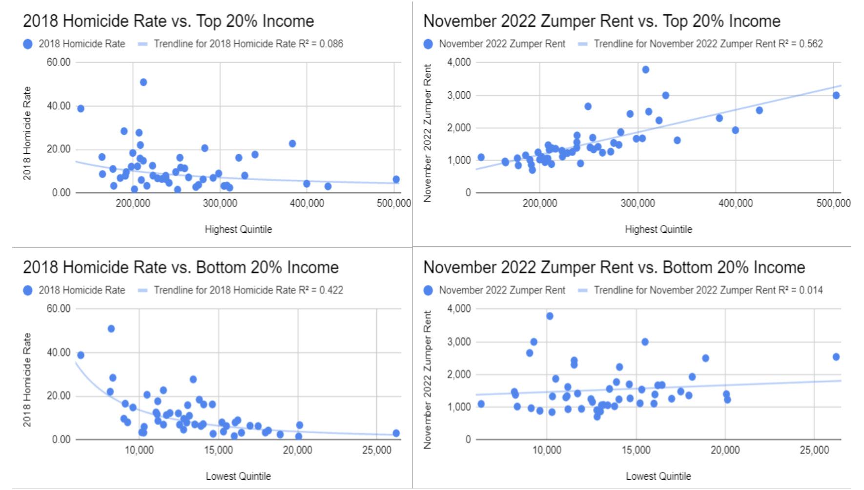
The data used for income is census data for the average income (after transfers, before taxes) of members of the top 20% and the bottom 20% of each of the top 50 largest cities in the US. The Zumper National rent report provided the data for typical one-bedroom apartment rents. The homicide rate data for the 50 largest cities in the country was sourced from Macrotrends.com (Note: unfortunately, 2018 was the most recent year with data), which in turn sourced it from the FBI (Macrotrends.com was used rather than directly sourcing from the FBI because Macrotrends.com formats data in a more usable format than the FBI). The homicide rate was used as a proxy for crime because homicide data is the most comparable crime across municipalities due to everyone defining homicide the same way unlike some other crimes which are more subjective in nature and would make for bad data. For example, the precise definition of a robbery differs by city based on local laws. It leads to the official crime statistics being a bit different in two cities with the same level of robberies, and a similar effect for other crimes. Homicide, on the other hand, is measured by every city using the same straightforward definition. Homicide rates tend to be higher in cities where crime is overall higher, such as Philadelphia and Chicago. Therefore, using this standardized measure as an overall proxy for crimes should be valid.

The homicide rate and rent datasets were merged with the income percentile dataset to investigate how the income of the top 20% and bottom 20% of a city correlate with the given city’s typical rent and homicide rate. Rent prices were predicted extremely well by how much people on the top of the economic spectrum in a given city made. Typical rent was predicted far better by the income of the top 20% of households than by the income of the bottom 20% of households. This is likely because the top 20% of households in a city can bid up the rent as much as they want, whereas lower-income households can’t bid up rent (Arefava, 2016). On the other hand, crime was extremely well predicted by how little people on the bottom of the economic spectrum in a given city made. Homicide was predicted far better by how much the bottom 20% of households earned than by how much the top 20% of households earned. This is likely because most crime is committed by people on the lower end of the economic spectrum (Patterson 1991). Because rent is correlated positively with the income of the top 20% and crime is correlated negatively with the income of the bottom 20%, it seems logical that the larger the gap between the top 20% and bottom 20% the higher rent and crime will be. With a high income gap, the rich will be “rich” enough that they massively bid up rent prices, and the poor will be so “poor” they commit lots of crimes. Major cities have lots of income inequality, with a vast gulf between the top 20% and the bottom 20% , it thus makes sense that major cities have high rent and high crime rates.

The most common way to measure income inequality is the Gini coefficient (Catalano, Lesie, & Pfaff, 2009). It is a number ranging from 0 to 1, where 0 is perfect equality and 1 is a single entity controlling all of a given resource. The census calculates the Gini coefficient of income inequality for each city in the US, and this dataset was merged with the previous two in order to investigate the relationship between income inequality and a measure of combined standardized rent and homicide rate. This combined standardized measure was created by adding the Z score of each city’s typical rent value and the Z score of that city’s homicide rate (Z score is a statistical method for standardizing data). When comparing this combined standardized measure of rent and homicide rate, the average income of people in the middle-income quintile of the R2 is nearly zero (0.021). However, if the urban cores of metropolitan areas with over 4 million are isolated, it is clear that the measure is higher in those cities than in the others (1.095 vs -0.426). There is clearly something driving this standardized measure of rent and homicide to be higher in big cities, and it may not be the income of a typical household since the correlation with the income of a typical household is nearly 0. The Gini coefficient was predictive of cities’ combined standardized rent and homicide rate (R^2 of 0.427), and

both of these stats are particularly high in the urban cores of the largest metropolitan areas in the country. Income inequality, rather than absolute income, best predicts rent and homicide in big cities.

The average Gini coefficient in urban cores of metropolitan areas with over 4 million people is 0.5268, compared to 0.4733 for other cities in the top 50. This may not appear to be a large gap on the surface; however, it is a gap of more than one standard deviation (the standard deviation for Gini coefficient of the 50 largest cities in the US is 0.0336). Using a two tailed unpaired t-test, the p-value for this difference is less than 0.0001, meaning the difference in mean Gini between large urban cores and other cities is statistically significant. The average combined Z score of rent and homicide rates in urban cores of metropolitan areas with over 4 million people is 1.0952, for other cities in the top 50, it is -0.4259. Using a two tailed unpaired t-test, the p-value for this difference is less than 0.0001; in other words, this difference between urban cores of metropolitan areas with over 4 million people and the other cities is also very statistically significant. Although it requires more rigorous methods to prove casualty, it seems that how expensive and dangerous a city is has to do with not just how much income there is but how that income is distributed. Our nation’s largest cities are currently in population decline due to being both expensive and dangerous, and this likely has to do with the fact that income is distributed very unevenly in those cities. If our nation’s major cities want to reverse this decline, they should likely look at reducing this trend of massive income inequality.

REFERENCES

Arefeva, Alina. “How Auctions Amplify House-Price Fluctuations.” Stanford University, February 2016.

Catalano, Michael T., Tanya L. Leise, and Thomas J. Pfaff. “Measuring Resource Inequality: The Gini Coefficient.” Numeracy 2, Iss. 2 (2009): Article 4.

Patterson, Britt E. “Poverty, Income Inequality, and Community Crime Rates.” Criminology, November 1991.

Data Citation

https://censusreporter.org/tables/ B19081/ https://censusreporter.org/tables/ B19083/ https://www.zumper.com/blog/ rental-price-data/ https://www.macrotrends.net/cities/us/md/Baltimore/murder-homicide-rate-statistics