TABLE II: KMO AND BARTLETT’S TEST

1) Test Results

χ2 = 2470.514; df = 153; p<0.0001

2) Statistical Decision

The null hypothesis that the correlation matrix of the variables is not significantly different from an identity matrix was rejected since the p-value was 0.0001 was less than 0.05 level of significance. This implied that the correlation matrix of the variables is significantly different from an identity matrix, and thus the sample correlation matrix did not come from a population in which the correlation matrix is an identity matrix. If the KMO statistics exceed 0.6 and Bartlett’s test of sphericity is statistically significant (p-value is less than 5%), then PCA is usually recommended for analysis. “A Kaiser-Meyer-Olkin measure of sampling adequacy that is greater than 0.7 is regarded to be a good sign that PCA is useful for the variables under consideration, according to the rule of thumb”. From the results in Table II, the correlations matrix was appropriate for component analysis because the KMO statistics was 0.865, which was more than the recommended 0.7. The Bartlett’s Test in Table II was precisely sufficient for the data under study. This is because Bartlett’s Test of Sphericity was used to test the difference between the correlation matrix for variables and the identity matrix was 2470.514. This showed that there was a significant difference. As a result, the correlation matrix for the measured variables differed significantly from the identity matrix and so remained consistent with the matrix’s factorable premise.

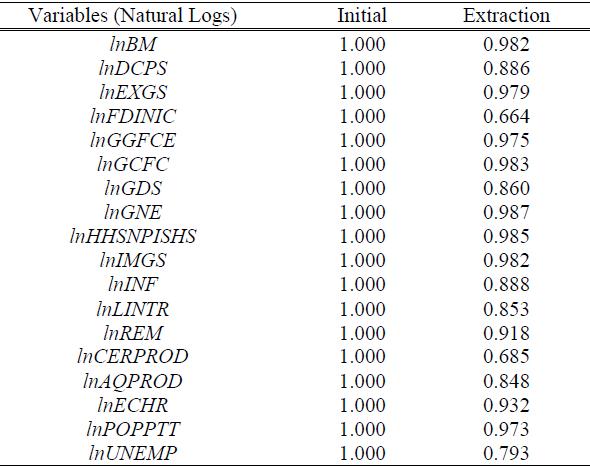
C. Communalities

The sum of the squares of the loadings of the iit variables on the ‘n’ common components, that is, the iit commonality, was carried out in the results presented in Table III.

Extraction Method: Principal Component Analysis.

All the macroeconomic indicators ranging from Broad money to total unemployment had a similar pattern and were highly correlated since the communalities of each indicator were greater than 0.65.

Furthermore, all the variables highly influence economic growth under the study period, as indicated by the high correlation.

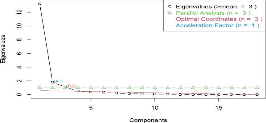
D. Scree Plot and Parallel Analysis

The scree plot and parallel analysis to help in the determination of the principal components to be retained were carried out, and the results are presented in Fig. 1.

Fig.1. Scree plot.

To visually examine the Eigenvalues for inflection points, we used the Scree test. The visual representation looks to have a downward slope after the third PC, indicating that the three preceding PCs may be precisely summarized to be reflective of the variables in totality. As seen in the scree graphic, the use of Eigenvalues retrieved three principal components from the data. In addition, we used parallel analysis to avoid over-and under-extraction. After parallel analysis, three components were chosen for further examination. The three components extracted and retained are a representation of all the original variables. Each of the three components contains a number of original variables. However, the number of original variables differs from one component to another. The number of variables in each component was identified using the rotated component matrix.

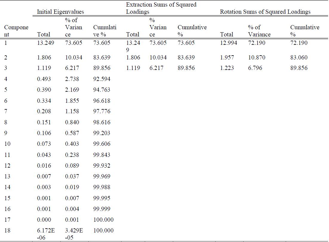
E. Total Variance Explained

The eigenvalues were used to carry out a test of the variation of the components, and the results are summarized in Table IV.

From Table IV and considering the eigenvalue-one criterion, the first component explained 73.61 percent of the overall Variance while the second one explains about 10.03 percent of the total Variance. The 3rd, 4th, 5th, 6th, and 7th PCs explained around 6.217%, 2.74%, 2.17%, 1.86%, and 1.16 percent of the total variation, respectively. The remaining components described less than one percent of the total Variance each. Clearly, the first component explained the largest variation, and as we progress from one component to the next, a descending trend emerges. Additionally, both the first and second components cumulatively explained approximately 83.64 percent of the overall Variance. By employing the orthogonal Varimax technique to produce the uncorrelated factor structures, the study found that the summarized total variation in the original set of data variables per the three retained components was about 89.86%.

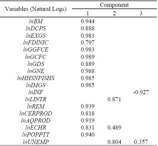
F. Rotated Component Matrix

The rotating component matrix aids in the decision-making process. It includes the calculated correlations between each variable as well as the estimated main components. It comprises the calculated main components as well as the estimated correlations between the variables. As shown in Table V, the Rotated Component Matrix displays the loadings for each item on each rotating component.

TABLE V: ROTATED COMPONENT MATRIX

Table V indicates that component 1 was highly correlated with 15 original variables, which included; broad money, domestic credit to the private sector, gross capital formation, population total, exports of goods and services, general government final consumption expenditure, foreign direct investment-net inflows, personal remittances received, gross domestic savings, gross national expenditure, aquaculture production (metric tons), households and NPISHs Final consumption expenditure, imports of goods and services, imports of goods and services, cereal production (metric tons), and official exchange rate. This component mostly resembles the monetary economy, the trade and openness of the economy with government activities, the consumption factor of the economy, and the investment factor of the economy. Likewise, the lending interest rate and total unemployment (percentage of the total labor force) had a higher positive loading into the second principal component. This component is closely related to both the labor economy and the monetary economy. Finally, the third principal component was highly correlated with only one of the original variables that is Inflation. This component resembles the trade and openness of the economy. Graphically, this can be presented using a biplot and factor analysis and a graph of variables.

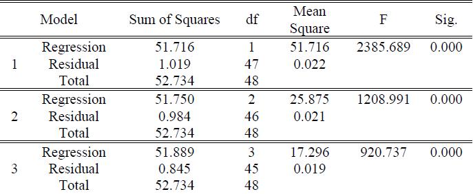
G. Hierarchical Regression Model

The hierarchical regression model was conducted to examine the effect of the predictor variables on the predicted variable. Three models were fitted, and the results are summarized in Table VI.

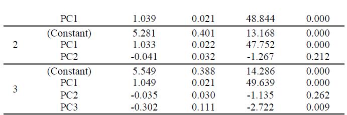
TABLE VI: ESTIMATES OF PARAMETER IN MODELS

In order to determine the association between the first component (with 15 original variables), the second component with two variables, the third component with only one original variable, and the GDP (dependent variable), the researcher conducted a hierarchical multiple regression analysis as presented in Table VI. As per the R generated output, the equation (�� = ��(����1, ����2, ����3) + ��) successively becomes;

In (19), the coefficient of the second component was negative and insignificant. Similarly, in (20), the coefficients of the second component were negative and insignificant, while the third component was negative and significant. After the insignificant coefficients were dropped, the retained coefficients formed (21), (22), and (23).

The constant terms, which are also the intercepts of the three models, were 5.086, 5.281, and 5.549, respectively. They showed an increasing trend as more components were added to the respective models, as shown in Table VIII. Since the t - values obtained had p - values of 0.000, which were less than the critical value of 0.05, all three constants were significant. The values 5.086, 5.281, and 5.549 are the values of GDP that do not depend on the macroeconomics variables (independent variables). The first component that contained 15 original variables and the gross domestic product was positively and significantly associated because the t value (48.844) attained had a p-value less than the 0.05 critical value (coefficient of X1 = 1.039, p = 0.000). This means that a unit increase in the first principal component holding other components constant would lead to an increase in GDP by 1.039 units, and the influence was significant. Further, after the addition of the second principal component (with two original variables), the results indicated that the first principal component and GDP were positively and statistically significantly related, whereas the second component and economic growth had a negative but the relationship was not statistically significant. This was supported by the t values of 47.752 and1.267 with their corresponding p values of 0.00 and 0.212, respectively. The coefficient of the first principal component was 1.033, while the second one had a coefficient of -0.041. This implied that a unit increase in the first principal component results in an increase in Kenya’s GDP by 1.033 units but GDP decreases by 0.041 units as the second component increase by one unit.

Finally, the third model included all the three extracted principal components as per the original variables. The first component was found to have a significant positive relationship with the GDP while the second one had a negative, but its relationship with economic growth was not statistically significant since its p-value (0.262) was greater than the five percent level of significance. The third component was found to have a significant negative association with the GDP. Additionally, the first component had the greatest influence since its unit increase resulted in a 1.049 unit rise in Kenya’s GDP. The second principal component had a coefficient of -0.035 with a p-value of 0.262, indicating that GDP decreases by 0.035 units as per unit increase in the second component, but the influence was insignificant. The coefficient of the last component was – 0.302 with its corresponding p-value of 0.009 and thus having an inverse relationship with the GDP. This shows that an increase in the third component by one unit would lead to GDP significantly reduced by 0.054 units.