Introduction
1 What Is Forensic Chemistry?
2 Precedent in Chemistry and the Law
3 Key Forensic and Legal Concepts
4 The Flow of a Forensic Analysis
OVERVIEW AND ORIENTATION
5 The Forensic Mind-Set 6 Forensic Chemistry Today 7 Becoming and Being a Forensic Professional
Forensic chemistry exists where science and the law overlap. You might expect the marriage of science and the law to be an easy and natural one, but frequently it is not. The widespread perception is that science and the judicial system both exist to seek the truth, but that is an incomplete description. Although tackling the definitions of scientific and legal truth is beyond the scope of this book, their intersection is at the heart of it, even when hidden behind chemical equations and reaction mechanisms. The term forensic refers to law enforcement, the judicial system, and the courts, and without forensic, there is no forensic chemistry. Accordingly, this brief chapter will provide you with the minimum legal context needed to explore forensic chemistry and the larger world of forensic science.
1 WHAT IS FORENSIC CHEMISTRY?
Forensic chemistry is applied analytical chemistry. If that were the extent of it, however, there would be no need for a separate course or textbook on the subject. What then makes forensic chemistry unique? Arguably, it is the same consideration that defines forensic science as a distinct discipline: the skill, art, and science of comparison. Analytical chemistry encompasses qualitative and quantitative analysis, but forensic chemistry adds comparative analysis to the task list. For example, spectroscopic analysis can quickly determine whether a fiber is made of nylon or whether a piece of plastic is polyethylene. These are analytical descriptors that answer analytical questions such as, What is it? and How much of it is there? Analytical chemistry provides qualitative and quantitative data that are required to answer forensic questions such as the following:
• Where could this fiber have come from?
• Could this piece of plastic have come from this plastic trash bag?
• Was weathered gasoline used to start this fire?
• Did this paint chip come from that car?
From Chapter 1 of Forensic Chemistry, Second Edition. Suzanne Bell. Copyright © 2013 by Pearson Education, Inc. All rights reserved.
Introduction
• Does this white powder contain a controlled substance?
• Do the quantities of drugs and metabolites found in these postmortem samples allow for determination of a cause of death?
The forensic question is often not the same as the legal question. For example, if a drug analysis section receives a white powder as evidence, the forensic question is probably, Does this white powder contain a controlled substance? If so, what and how much? The chemist performs the analysis and provides data such as “The sample was found to contain cocaine as the hydrochloride salt. The net weight of the powder was 6.234 g ± 0.012 g.” This statement provides a concise answer to the forensic question but not the legal question, which is probably, Is the defendant guilty of felony possession of a controlled substance? The forensic chemist has supplied data that can contribute to answering this question, but only a piece of the total answer. It is good practice to keep this distinction in mind.
A
The Origins of Science and Chemistry
Ancient chemistry was likely related to medicines and materials. Knowledge was based on experiment and experience and was passed on to a select few. Early humans used plant and animal products as treatments and learned from experience what worked and what did not, but there was no understanding of natural laws (i.e., science) to guide them. The Greeks were the first to set forth the idea of science as a system or method of looking at the world, and this system began to take shape 2500 years ago. By that time, chemistry was already well established in certain areas, including natural dyes, simple metallurgy, soapmaking, cosmetics, fermented beverages, and ceramics. The Greeks created a philosophy that allowed knowledge derived from experiment to be studied systematically and then extended logically to new situations.
Source: Salzberg, H. W. “Ancient Technology: The Roots of Chemistry,” in From Caveman to Chemist: Circumstances and Achievements. Washington, DC: American Chemical Society, 1991, 1–15.
When a forensic scientist works with an exhibit of evidence, generally there are three tasks to be accomplished. First is identification. In drug analysis, this task incorporates qualitative identification and, sometimes, quantitative analysis. In other cases,
EXHIBIT B
Live by the poison, die by the poison
The Greeks may have formulated the idea of science, but it was the practical Romans who formulated the first essential elements of forensic science. One of the most common, most feared, and most difficult crimes to detect in the ancient world was poisoning. A very early law outlawing this crime was set forth by Rome in 82 B C. Nearly 250 years prior to that, the Romans had executed a number of women convicted of poisoning husbands, fathers, other relatives, and significant others. The women were executed by being forced to drink their own concoctions, leading to various versions of the title quotation. The word forensic is tied to the Latin word forum, a place where the Romans conducted business and legal proceedings. To speak in the forum was to speak the truth (or so it was hoped or assumed), leading to the link between forensic and modern debate teams. However, the word also refers to speaking the truth in public, a good job description for forensic chemists.
EXHIBIT
Introduction
such as fiber analysis, identification is the easy part. The next step is classification of the evidence. Is the fiber nylon 6 or nylon 66? Is it red, yellow, or blue? Has it aged? What is its cross section? The answers to these questions reduce the size of the class to which the fiber belongs. The smaller the class membership, the more meaningful is the evidence. Taken to its logical conclusion, classification results in placing the fiber in a class with only one member. This process is referred to as individualization or establishing a common source, although this terminology seems to be losing favor in the forensic community. Regardless, the concept is a useful one, even if reducing the number of possible sources to a single entity is rarely possible.
Continuing with this example, assume that a fiber is found at a crime scene. The forensic analyst determines that it is a red nylon fiber with a circular cross section. A suspect wearing a red nylon windbreaker is arrested. Nylon fibers from the windbreaker (often labeled K for “known”) are subjected to the same tests as was the fiber in question (Q) from the scene, with similar results. The analysis demonstrates that Q and K belong to the same class, but this is not proof of a common source. Rather, this is an example of inclusive evidence (described below). In other words, the test fibers from the jacket and the fiber from the crime scene have not been individualized, and the analyst cannot assign a common source (the jacket) to Q and K. This does not mean that the evidence is useless, but it does limit what can be said with confidence. The jacket is not excluded as a possible source.
Drug analysis, both of physical and biological evidence, falls outside the traditional forensic framework of identification–classification–individualization. Analytical instrumentation, properly applied, nearly always allows for the unambiguous identification of a chemical compound, be it a drug or metabolite. Classification involves presumptive testing and screening tests, but identification follows classification rather than preceding it, as in the case of our hypothetical fiber. Identification, classification, and individualization are all involved in forensic chemistry, even if the order varies.
2 PRECEDENT IN CHEMISTRY AND THE LAW
Science exists to uncover a deeper understanding of the universe, guided by the principles of the scientific method. The tools used are experimentation and observation. Courts exist to settle disputes between individuals and the state (criminal law) or among individuals or entities (civil law). Courts are guided by the law, precedent, and function using an adversarial system. It would be a mistake to assume that the courts use a model similar to the scientific method or that science works on the basis of argument. There are elements of each in both systems, but to the forensic chemist, the differences are as important as the similarities (Figure 1).
Both science and the courts are tasked with deriving information from evidence pertinent to the issue at hand. Science employs the scientific method to do so, whereas the courts employ the adversarial system, in which two opposing parties present arguments before the trier of fact. Scientific evidence and testimony may support or refute either argument. The relative strengths of the arguments guide the court in settling the issue. Scientific knowledge and findings are part of that process, but only part. All scientists can and should do is produce the best science possible, followed by making the clearest presentation possible. How the data are used is for the courts to decide. Many such decisions are based on precedent, or that which has gone before. When a precedent is created, new rules or new applications of rules to decide a case or issue are developed and used.1 Precedent is a guide for decisions and is based on past lessons. In that sense, precedent is knowledge gained previously in similar settings. Science also invokes the concept of precedent, since new ideas are derived from previous observations and experiments.
Models and understanding of the natural world
Truth Settles disputes
1 Different paths toward similar, but not identical, destinations.
FIGURE
EXHIBIT C
The Origin of Law
The Greeks and the Romans could not have made their contributions to forensic science had it not been for a much earlier invention: the law. The first-known codified laws were put forth by the peoples who occupied the Tigris and Euphrates River valley areas in what were the earliest-known cities and civilization. The earliest-known laws and legal systems appeared around 2000 B C. Arguably, the most famous was Hammurabi’s code, named for the Babylonian king in power around 1700 B C
3 KEY FORENSIC AND LEGAL CONCEPTS
This is a chemistry text first and foremost, but because it is a forensic chemistry text, brief mention of the discipline’s legal foundation is in order. The central precepts applicable to forensic chemistry are summarized in the paragraphs that follow, and the “Further Reading” and “References” sections at the end of the chapter list additional resources.
3.1 Criminal and Civil Cases
Forensic chemists working in local, state, and federal laboratories are usually involved in criminal cases. Criminal law deals with crimes by a person or persons against the state, which can be any level of government, including cities, counties, states, and the federal government.1 Civil cases arise from disputes that involve private rights or from disputes such as those between two individuals or two corporations. Cases referred to informally as lawsuits, wherein the complainant is said to be “filing suit,” involve civil law.
3.2 Admission of Evidence
The history of the admissibility of scientific evidence in the United States is surprisingly short, less than a century old.2 To date, standards of admissibility are founded on four court rulings, and their application varies with the jurisdiction.
The Frye Rule (general acceptance): This standard of admission was established in a 1923 case heard in the District of Columbia Circuit Court: Frye v. United States, 293 F. 1013, 1014 (D.C. Cir. 1923). Distilled to its essence, the court’s ruling held that evidence produced by scientific analysis is admissible as long as the techniques are accepted as valid by the relevant scientific community.3 In effect, the court said that if the test has survived the rigor of the scientific method and peer review to reach the status of general acceptance, then it has already been tested and validated. For example, if a new technique was developed for the chemical characterization of dyes in ink, the results of tests performed in accordance with that technique would not be admitted under the Frye rule unless the court determined that analytical and forensic chemists generally recognized the technique as useful and reliable. The Frye standard was predominant into the early 1990s and is still used in some jurisdictions.
The Daubert Decision: This ruling, handed down by the U.S. Supreme Court (Daubert v. Merrell Dow Pharmaceuticals (113 S.Ct. 2786 (1993)), was based on the Federal Rules of Evidence enacted in 1975. The case focused particularly on Federal Rule 702. The decision in Daubert gave judges what is referred to as a gatekeeper in determining admissibility.
Introduction
Although this decision applied only to federal cases, several states have adopted the same approach to admissibility.
Daubert has had a significant impact on forensic science in the past decade, particularly in the realm of DNA evidence, which came of age under this decision. The Daubert decision provided judges with a list of tools and tests that could be used to determine the admissibility of evidence. General acceptance by the relevant scientific community is one of these, but a host of others were put forward including testability of the method, peer review (e.g., publication in peer-reviewed journals), existence of standards that can be used to test the method, and the existence of known error rates. In cases where admissibility is an issue, judges can convene admissibility hearings (also called Daubert hearings) to determine the merit of the method. The rigor required for acceptance under Daubert and the role of Daubert in hearings that determine admissibility are forcing a reexamination of forensic mainstays such as fingerprint evidence. No doubt forensic chemistry will be affected as this situation evolves.
General Electric v. Joiner (522 U.S. 136 (1997)): This case was the second of what is now called the Daubert trilogy. In this case, the issue was related to workplace exposure to hazardous chemicals (PCBs) and the outcome was clearly going to depend heavily on which scientific studies were admitted. In terms of admissibility, the ruling in the case stressed the need to weigh the relevancy of the data to the question at hand. For a method or technique to be considered admissible, it must be clearly and unambiguously pertinent to the question at hand.
Kumho: Daubert was extended by the 1999 decision in Kumho Tire Co., Ltd. v. Carmichael (119 S. Ct. 1167 (1999)). This ruling, which completes the trilogy, extended the scope of Daubert and the judge’s gatekeeper role to all expert testimony, not just scientific. The decision also acknowledged that standards for determining admissibility would differ, depending on the discipline in question.3
3.3 Inclusive versus Exclusive Evidence
Often, forensic chemists produce scientific evidence that can be described as either inclusive or exclusive. Recall the red fiber example mentioned earlier in the chapter. In that example, successive classification based on analytical data demonstrated that the red fiber from a crime scene belonged to the same class as fibers from a suspect’s red nylon jacket. This is an example of inclusive evidence: the jacket is included in the population of items that could have been the source of the fiber in question. Had the fibers from the jacket been found to have a cross section different from that of the fiber found at the scene, they would have been exclusionary evidence: The jacket could not have been the source.
3.4
Direct and Circumstantial Evidence
Direct evidence is that which is known to a person by personal knowledge, such as eyewitness testimony. Such evidence, if found to be true, would prove a point in contention without requiring any additional analysis or inference. 3 Forensic scientists, by contrast, produce circumstantial evidence, or evidence that requires inference to move logically from the information provided to the answer to a question. For example, if blood is found on a knife, and DNA typing showed that the blood matched that of a suspect, with a probability of 1 in 6 trillion, the trier of fact must still infer that the blood came from the suspect, since the deposition of the blood was not directly witnessed. Contrary to popular belief, circumstantial evidence is not, by definition, weak evidence.
3.5 Chain of Custody
The “chain” as it is called, is a paper form that tracks evidence from its creation or collection to its final disposal. A “cradle-to-grave” document that completely describes the history of a sample or an exhibit constituting evidence, the chain is initiated when the sample is collected or created and is updated each time the sample is transferred from one person to another. The chain ensures that the sample’s history has no gaps and that the sample was in the direct control of one person at all times, though not always the same person. When a sample is in the laboratory, it either is stored in a secure, locked storage area or is being analyzed. Any break in the chain, no matter how innocent or inadvertent, raises the possibility that the sample could have been tampered with. Accordingly, painstaking steps are taken to ensure the integrity of all evidence. Among these steps are establishing security measures, guaranteeing controlled access to storage areas, and implementing specific protocols for opening, marking, sealing, and transporting evidence. Maintenance of the chain is a fundamental responsibility of any forensic analyst.
3.6 Destructive Testing
If an exhibit of evidence is consumed in testing, the tests performed on it can never be repeated or verified. Although this is not a limitation when the case consists of several milliliters of blood or a large bindle of white powder, other cases are not so simple. If the exhibit is a single fiber or one tiny paint chip, analytical options are limited. Solubility tests would be a poor choice for a single paint chip, but microspectrophotometry (nondestructive) would be ideal.
Applying the Science 1 The Power of a Common Source and Circumstantial Evidence
The Wayne Williams case was made without eyewitnesses, without DNA, and without fingerprints. In 1982, Wayne Williams was convicted of murdering 2 young boys in Atlanta, but he was likely responsible for the killings of at least 10 others. The key evidence in the case was fibers and dog hair that represented an accumulation of circumstantial evidence the jury could not ignore. In 11 of 12 fiber correlations, fibers found on the victims and in Williams’s home or car were determined to be members of the same small class. Any one of these 11 correlations was inclusive evidence, but when they were considered together, the chances that 11 different fiber or hair types would be found both on the victims and in Williams’s environment were too small for the jury to consider as coincidence.
Source: Deadman, H. A. “Case Reading: Fiber Evidence and the Wayne Williams Trial.” In Criminalistics: An Introduction to Forensic Science, ed. R. Saferstein. Upper Saddle River, NJ: Prentice Hall, 2004.
4 THE FLOW OF A FORENSIC ANALYSIS
It is important to understand that forensic chemists work on the basis of a finite universe of substances that are of interest. The method selected must answer the forensic question, such as, Does this fire debris sample contain an accelerant? The forensic question dictates the method, which must be fit for the purpose of detecting accelerants. The chemist (and the legal system) is not interested in determining what kind of wood was in the fire or what other materials are present—only whether there was an accelerant. Similarly, in forensic toxicology, the universe of analytes consists of drugs, poisons, and their biotransformation products. If a postmortem blood sample arrives at the
laboratory, the toxicologist will not apply a method to determine the cholesterol level in the blood, because that information is not relevant to the case at hand (as per the Joiner decision). Such a method would not be fit for the purpose of detecting drugs, poisons, and metabolites. You should keep this in mind as we begin to delve deeper into the specifics of different analyses. A forensic analysis is usually a narrowing-down process, as shown in Figure 2 . Although the sample matrix may be known (blood, urine, fire debris, etc.), many samples are complex mixtures that require a systematic approach to characterize them. Generically, a forensic chemist relies on three groups of techniques: visual examination and inspection (both macroscopic and microscopic), organic chemical analysis, and inorganic chemical analysis. The sample or exhibit of evidence is often referred to as a general unknown, even though the analyst usually has some idea of what is or might be present in the sample.
Presumptive tests
All possible components
Definitive identification
Analysis starts with qualitative presumptive tests that narrow down the list of potential analytes and direct subsequent analysis. In some cases, visual or microscopic examination suffices as a first step. Presumptive tests utilizing chemical reagents belong to a family of analytical techniques referred to as wet chemical methods. Most are based on observing results when specific reagents are added to small portions of the samples. Color and crystal tests, as they are commonly called, are used in analyzing drugs, gunshot residues, and explosives. These tests will be discussed in detail in subsequent chapters. It is worth noting that as instrumentation improves and becomes more affordable, there is decreasing reliance on wet chemical methods; however they will continue to play a role for the forseeable future.
Once presumptive tests have focused the analysis on a small set of potential components, the next step usually involves the separation and isolation of target components, either for screening tests or for definitive identification. Typically, such steps involve extraction and chromatography. Forensic chemists often employ thin-layer chromatography (TLC) in the analysis of inks and drugs as a follow-up to presumptive tests, whereas toxicologists may use immunoassay to narrow the field of potential analytes. Chromatography can also be employed for sample cleanup and analyte isolation, as can solvent extractions, headspace methods, and solid-phase extractions. Confirmation of tentative identification follows, using instrumental techniques such as infrared spectrophotometry and gas chromatography–mass spectrometry (GC-MS). The latter is particularly valued because of its capabilities in separating, identifying, and quantitating analytes, although the degree of quantitative analysis required varies. In seized drug analyses, GC-MS is often the primary analytical instrument used, whereas for other purposes, such as analyzing fibers, it may be less important or even inapplicable.
As we discussed previously, the majority of forensic chemical analyses do not require the complete characterization of a sample. For example, a small resinous cube of brown material may be found to contain heroin along with many other materials; however, analytical interest usually ends with the identification of the illegal drug or substances. Occasionally, the materials used as cutting agents (diluents) are identified, but that is usually the extent of the testing. Although a complete characterization could be invaluable for linking the resin to others and for determining origins, testing for such purposes is not routinely performed, given the time and expense required. Like all analytical chemists, forensic chemists balance the need for accuracy, precision, and completeness against the reality of limited time, money, and resources. The overriding
Screening tests
Quantitative analysis
FIGURE 2 The flow of a forensic analysis.
consideration is always how well the method answers the forensic questions. The next chapter describes the acceptable compromises that yield useful, reliable, and legally defensible data.
5 THE FORENSIC MIND-SET
There is a core set of skills that any forensic scientist should cultivate as part of a forensic mind-set. The importance of comparison in forensic analyses imposes conditions on methods selected, how they are applied, and how the results are interpreted. Consider a case in which the forensic chemist is provided a tiny fragment of a thick, fibrous, silvery material with one adhesive surface. The evidence is the only remaining trace of the material that was used to bind a homicide victim. A suspect has been identified and a search of his house reveals three different rolls of duct tape. The forensic question is, From which roll, if any, could the fragment of tape have come? The identification part of analysis is simple: A quick look through a stereomicroscope shows the material to be duct tape. The challenge is how to proceed, given that the evidence cannot be destroyed.
If the analyst is lucky, it may be possible to physically match the fragment to one of the rolls (identifying a common source, or individualization). If not, the tape can be examined microscopically and with microspectrophotometry. Careful study of the fiber pattern in the tape, combined with some database searching and phone calls, may narrow the possible manufacturers of the tape (classification). A trip to the library (a building or an electronic repository) may uncover an article in a forensic, analytical, or industrial journal (e.g., Journal of Forensic Sciences, Forensic Science International, Canadian Journal of Forensic Science, Adhesives Age, or Adhesives and Sealants Industry) that describes how others have approached similar problems. Experimentation with tapes unrelated to the case can further refine the approach. Although this kind of case is not routine, it highlights the skills that constitute the forensic mind-set. Forensic scientists and forensic chemists should
• assume nothing.
• be resourceful. Finding at least two journals devoted to adhesives would be of significant help in the case and would take only minutes via an electronic search. Browsing articles could produce names of experts in adhesives to contact for assistance.
• think outside the discipline. Forensic science integrates many areas, chemistry being only one, but the core skills and principals of science are always the same. The analyst in this case would probably find reading adhesives journals easier than expected.
• be creative. Often, creativity is attributed to the arts (painting, music, etc.), but successful scientists and researchers must be creative as well. Creativity involves applying a novel approach to a problem or finding a novel application of existing tools and skills. All painters use paint, but there are an infinite number of ways to assemble the colors on a canvas. Similarly, all analytical chemists have access to the same set of tools; it is how they are applied that makes an approach creative. Challenging cases require creativity.
• build a big toolbox that never stops growing.
• know their limitations and never speak beyond what their data and expertise support.
• be flexible. Just because something works in this case does not necessarily mean that it will work in the next one. The more knowledgeable and resourceful a scientist is, the more flexible he or she is.
• be persistent. The case described in this section might at first glance have seemed hopeless to the analyst, but it was not. Difficult is not the same as impossible; a good forensic scientist recognizes the difference.
6 FORENSIC CHEMISTRY TODAY
Analytical chemistry in the forensic field is generally divided into two areas: forensic toxicology and forensic chemistry. The divisions are somewhat artificial, but an understanding of them is important. Forensic toxicologists work with biological evidence and follow the trail of drugs and poisons ingested by humans or other organisms. Forensic toxicology is often associated with death investigation and the medical examiner’s or coroner’s office, depending on the jurisdiction. Certainly, forensic toxicologists are also forensic chemists; the division between forensic toxicology and forensic chemistry and the use of those job descriptors are rooted in history and tradition.
Forensic chemists work with physical evidence and are often employed in what are often called “crime labs,” although this term seems to be falling out of favor. In general, qualifications for employment in either type of laboratory (crime lab or toxicology lab) are a B.S. in a natural science (preferably chemistry) with an emphasis on analytical and instrumental methods. Entry-level toxicology positions may require additional training or experience in toxicology or pharmacology. The moniker “drug chemist” is sometimes used if the person works exclusively in that area; some forensic chemists work in trace evidence and other forensic specialties. Forensic chemists also work with materials such as inks, dyes, fire debris, gunshot residues, dusts, explosives, polymers, paints, and glass. If there is physical evidence and it is amenable to, and benefits from, chemical analysis, a forensic chemist or someone trained in that area can be involved in analyzing that evidence.
EXHIBIT D
The First Forensic Testimony
In truth, the first instance may never be known. It has been reported that a surgeon who examined Julius Caesar’s body was asked to testify as to which wound was fatal to the emperor. However, one of the first instances of modern forensic testimony was given by a chemist, M. J. B. Orfila (1787–1853), in a poisoning case. Orfila, held by many to be the father of forensic toxicology, was a prominent toxicologist and skilled chemist when the case of Marie LaFarge crossed his path in 1840. Marie LaFarge was a young French widow who, at 24, remarried. Her second marriage, to Charles LaFarge (age 30), was reportedly not a happy one. In 1839, Charles died after eating cake made by his wife; the symptoms were consistent with arsenic poisoning. Marie was charged and chemical tests were performed on the body, but the results were inconclusive. The court was unsatisfied and commissioned Orfila to journey from Italy to France to conduct a review of the scientific work in the investigation. Orfila eventually had Charles’s body exhumed. A skilled analytical chemist, Orfila was able to detect arsenic in the tissues. He also showed an appreciation for the need for control samples, testing the soil in which Charles had been buried and demonstrating that the arsenic did not originate from it. Marie was convicted and sentenced to involuntary servitude, during which time she wrote a book.
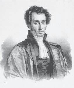

M. J. B. Orfila
Marie Lafarge National Library of Medicine
Mary Evans Picture Library/Alamy
7 BECOMING AND BEING A FORENSIC PROFESSIONAL
7.1 What Is a Profession?
Forensic science has evolved from an adjunct to medicine to a recognized profession— which raises the question, What defines something as a profession? A reasonable definition is that a profession is the practice of similar skills by a group of people who are paid to apply those skills in a more-or-less specified manner.4 A profession is differentiated from a job in that there is a governing body that oversees, regulates, and ensures that practitioners of the profession adhere to standard guidelines and meet certain minimum requirements. In a true profession, this regulation is derived internally, not imposed by an outside entity that does not practice the profession. For example, the American Medical Association (AMA) dictates how medicine is taught and practiced. The AMA works in concert with medical schools, hospitals, and government agencies, but, fundamentally, doctors dictate how doctors work and what the public can expect from physicians. Thus, a profession requires the existence of professional associations that have recognized and accepted authority within the profession.
7.2 Certification and Professional Organizations
A profession defines what prerequisites one must have and what minimal educational standards one must adhere to in order to participate in it. In forensic science, there are a number of professional organizations. The largest is the American Academy of Forensic Sciences (AAFS, www.aafs.org), founded in 1947. The AAFS is organized into sections such as jurisprudence, toxicology, criminalistics, and engineering. Of most interest to chemists are the criminalistics and toxicology sections. The AAFS specifies membership requirements and three levels of membership but does not certify individuals (although it is a partner in the process). The primary national professional organization for forensic toxicology is the Society of Forensic Toxicologists (SOFT, www.soft-tox.org). Certification of forensic toxicologists and accreditation of forensic toxicology laboratories is handled by the American Board of Forensic Toxicology (ABFT, www.abft.org). There is no single organization or association that deals exclusively with forensic chemists in the same way that SOFT and ABFT do with toxicologists. The American Chemical Society (ACS, www.chemistry.org) is the largest scientific society in the world and has sections devoted to analytical chemistry and just about every other chemical discipline imaginable. There is a section called “Chemistry and the Law,” but its scope includes things such as patent law—important, to be sure, but not directly forensic. The American Board of Criminalistics (ABC, www.criminalistics.com/abc/) offers certification of forensic scientists in several disciplines. General-service forensic science laboratories are accredited through the American Society of Crime Laboratory Directors LAB program (ASCLD, www.ascld.org).
Summary
Forensic science and forensic chemistry are young professions distinguished from other sciences by their relationship to the legal system and by the importance of comparison in laboratory analysis. Forensic chemists need an understanding of the legal foundation
of their chosen field, as well as a forensic mind-set, which relies on the fundamental precept of always being open to learning more and always adding tools to the toolbox. In that spirit, our journey into forensic chemistry can now begin.
Key Terms and Concepts
Admissibility hearing
Adversarial system
Chain of custody
Circumstantial evidence
Civil law
Classifications
Common source
Criminal law
Daubert decision
Daubert hearing
Problems FROM THE CHAPTER
Introduction
Daubert trilogy
Direct evidence
Exclusive evidence
Forensic question
Frye rule
Gatekeeper
General acceptance
General Electric v. Joiner
General unknown Identification
1. Compare and contrast the adversarial system and the scientific method. List the strengths and weaknesses of both in the context of criminal and civil law.
2. During a Daubert hearing, what entity ultimately decides on admissibility?
3. What role does peer review play in science and in the law? Compare and contrast.
4. Describe how a preponderance of inclusive circumstantial evidence can become conclusive in the eyes of a jury.
INTEGRATIVE
1. A great scientist can still be a terrible forensic scientist; a person who gives wonderful testimony can be a terrible
Further Reading
Bell, S. “Forensic Chemistry.” Annual Review of Analytical Chemistry 2 (2009): 297–319.
Bell, S. Crime and Circumstance: Investigating the History of Forensic Science. Westport, CT: Praeger, 2008.
Bliesner, D. M. Validating Chromatographic Methods Hoboken, NJ: Wiley, 2006.
James, S. H., and J. J. Nordby, eds. Forensic Science: An Introduction to Scientific and Investigative Techniques, 3d ed. Boca Raton, FL: CRC Press/Taylor and Francis, 2009.
References
1. Garner, B. A., ed. Black’s Law Dictionary. St. Paul: West Publishing Group, 2001.
2. Bell, S. “Admissibility and the Trilogy.” Chap. 18 in Crime and Circumstance. Westport, CT: Praeger, 2008.
Inclusive evidence
Individualization
Kumho
Legal question
Precedent
Relevancy
Trier of fact
Wet chemical methods
forensic scientist. Comment on these observations and their implications for forensic chemistry.
2. Can jurors ask questions of expert witnesses? Comment on your findings regarding this issue.
FOOD FOR THOUGHT
1. Is the analysis of drugs with instruments such as mass spectrometers and infrared spectrometry based on comparison?
2. How important is the way in which scientific evidence is presented? Comment on the relative importance of content versus presentation. Why is learning how to testify such an important skill?
Karch, S. B. A Brief History of Cocaine, 2d ed. Boca Raton, FL: Taylor and Francis, 2006.
Saferstein, R. Criminalistics: An Introduction to Forensic Science , 10th ed. Upper Saddle River, NJ: Pearson/ Prentice Hall, 2011.
Stajic, M. “Milestones of Forensic Toxicology,” in More Chemistry and Crime: From Marsh Arsenic Test to DNA Profile, ed. S. M. Gerber and R. Saferstein. Washington, DC: American Chemical Society, 1997.
3. Kennedy, D., and R. Merrill. “Assessing Forensic Science.” Issues in Science and Technology 20 (2003): 33–34.
4. Kovac, J. The Ethical Chemist. Upper Saddle River, NJ: Prentice Hall, 2004.
EXHIBIT A
Why Significant Figures Matter
In most states, a blood alcohol level of 0.08% is the cutoff for intoxication. How would a value of 0.0815 be interpreted? What about 0.07999? 0.0751? Should these values rounded off or are they truncated? If they are rounded, to how many significant digits? This is an artificial, but telling example. How numerical data are rounded depends on the instrumentation and devices used to obtain the data. Incorrect rounding might have consequences.
125.4 lbs 4 significant digits
FIGURE 2 Reading the scale results in four significant digits, the last being an educated guess or an approximation that, by definition, will have uncertainty associated with it.
Foundations
the data. The second point is to clearly distinguish between uncertainty and error. In the metrological context, error is defined as the difference between an individual measured result and the true value (i.e., accuracy).3 Thus, error and uncertainty are not the same and should not be treated the same, although both are important to making and reporting valid and reliable results. In this chapter, we will examine a simplified approach to calculating uncertainty. We will integrate additional information to generate more realistic and defensible estimates of uncertainty. Finally, keep in mind that the best we can do is estimate uncertainty; like a true value, it can never be known exactly.
2 SIGNIFICANT FIGURES, ROUNDING, AND UNCERTAINTY
Significant figures become tangible in analytical chemistry. The concept of significant figures arises directly from the use of measuring devices and equipment and their associated uncertainty. The rules of how significant figures are managed in calculations are covered in many introductory classes, so we will focus on the highlights here. However, you should review these rules to get the most out of this section. How that uncertainty is accounted for dictates how to round numbers resulting from what may be a complicated series of laboratory procedures. The rules and practices of significant figures and rounding must be applied properly to ensure that the data presented are not misleading, either because there is too much precision implied by including extra unreliable digits or too little by eliminating valid ones.3
In any measurement, the number of significant digits is defined as the number of digits that are certain, plus one. The last digit is uncertain (Figure 2), meaning that it is an estimate, but a reasonable one. With the bathroom scale example, one person might interpret the value as 125.4 and another as 125.6, but it is certain that the value is greater than 125 pounds and less than 126. The same situation arises when you use rulers or other devices with calibrated marks. Digital readouts of many instruments may cloud the issue a bit, but unless you are given a defensible reason to know otherwise, assume that the last decimal on a digital readout is uncertain as well.
Recall that zeros have special rules and may require a contextual interpretation. As a starting point, a number may be converted to scientific notation. If the zeros can be removed by this operation, then they were placeholders representing a multiplication or division by 10. For example, suppose an instrument produces a result of 0.001023 that can be expressed as 1.023 3 10 3. This demonstrates that the leading zeros are not significant, but the embedded zero is.
Trailing zeros can be troublesome. In analytical chemistry, the rule should be that if a zero is meant to be significant, it is listed, and conversely, if a zero is omitted, it was not significant. Thus, a value of 1.2300 grams for a weight means that the balance displayed two trailing zeros. It would be incorrect to record a balance reading of 1.23 as 1.2300. Recording that weight as 1.2300 would conjure up numbers that were useless at best and likely deceptive. If this weight were embedded in a series of calculations, the error would propagate, with potentially disastrous consequences. “Zero” does not imply “inconsequential,” nor does it imply “nothing.” In recording a weight of 1.23 g, no one would arbitrarily write 1.236, so why should writing 1.230 be any less wrong?
Another ambiguous situation that occasionally arises is associated with numbers with no decimals indicated. For example, how many significant figures are in 78? As with zeros, we need to know something about the context. If we are counting the number of students in a room, this is a whole, exact number. This number itself would not factor into significant figure determinations. The same is true of values such as metric
conversions. Each kilogram is comprised of 1000 grams. It’s not 1000.2 rounded down; 1000 is an exact number. If used in a calculation, you would assume an infinite number of significant figures; like 78 above, the number of digits plays no role in rounding considerations. In some analytical contexts, you may see notation such as 327. with a decimal point placed at the end of the number. This is done purposely to tell you that this number has 3 significant digits; it is not meant to represent a whole number or exact conversion factor. Finally, keep in mind that while metric conversions are based on exact numbers, not all conversions are. For example, in upcoming chapters, we will routinely convert body weights in pounds to kilograms. The conversion factor for that calculation is 1 pound 0.45359237 kilogram. It is up to you to decide how many significant figures are required for the calculation. When in doubt, keep them all and round at the end, but work on developing judgement skills that allow you to select the appropriate number. After all, the more digits kept, the more likely a transposition error. If you really do not need eight digits, do not use eight.
In combining numeric operations, rounding should always be done at the end of the calculation.3 The only time that rounding intermediate values may be appropriate is in addition and subtraction operations, although caution must still be exercised. In such operations, the result is rounded to the same number of significant digits as there are in the contributing number with the fewest digits, with one extra digit included to avoid rounding error. For example, assume that a calculation requires the formula weight of PbCl2:
The correct way to round or report an intermediate value would be 278.11 rather than 278.1. The subscript indicates that one additional digit is retained to avoid rounding error. The additional digit does not change the count of significant digits: The value 278.11 still has four significant digits. The subscript notation is designed to make this clear.
By definition, the last significant digit obtained from an instrument or a calculation has an associated uncertainty. Rounding leads to a nominal value, but it does not allow for expression of the inherent uncertainty. To do this, the uncertainties of each contributing factor, device, or instrument must be known and accounted for. For measuring devices such as analytical balances, autopipets, and flasks, that value is either displayed on the device, supplied by the manufacturer, or determined empirically. Because these values are known, it is also possible to estimate the uncertainty in any combined calculation. The only caveat is that the units must be the same. On an analytical balance, the uncertainty would be listed as 6 0.0001 g, whereas the uncertainty on a volumetric flask would be reported as 6 0.12 mL. These are absolute uncertainties that cannot be combined as is, because the units do not match. To combine uncertainties, relative uncertainties must be used. These can be expressed as “1 part per ” or as a percentage. That way, the units cancel and a relative uncertainty results, which may then be combined with other uncertainties expressed the same way (i.e., as unitless values).
Consider the simple example in Figure 3, in which readings from two devices are utilized to obtain a measurement in miles per gallon. The absolute uncertainty of each device is known, so the first step in combining them is to express them as “1 part per .” While not essential, such notation shows at a glance which uncertainty (if any) will dominate. It is possible to estimate the uncertainty of the mpg calculation by assuming that the odometer uncertainty of 0.11% (the relative uncertainty) will dominate. In many cases, one uncertainty is much larger (two or more orders of magnitude) than the other and hence will control the overall uncertainty.
FIGURE 3 Calculation of mpg (measurand) and an associated uncertainty estimate based on individual uncertainties from two measuring devices.
Better in this case is accounting for both uncertainties, because they are within an order of magnitude of each other (0.07% vs. 0.11%). Relative uncertainties are combined with the use of the formula:
For the example provided in Figure 3, the results differ only slightly when uncertainties are combined, because both are close to 0.1%, so neither overwhelms the other. Equation 1 represents the propagation of uncertainty (also called propagation of error in older references). The changeover from the “error” model to the uncertainty model occurred in the 1990s. It is useful for estimating the contribution of instrumentation and measuring devices to the overall uncertainty, but this approach is too simplistic for most forensic applications. For example, suppose some amount of gasoline in the preceding example overflowed the tank and spilled on the ground. The way you do the calculation does not capture this type of problem. The resulting calculation would be correct but not reliable. Spilling gasoline is the type of procedural error that is detected and addressed by quality assurance. In turn, quality assurance requires an understanding of the mathematics of multiple measurements, or statistics.
EXAMPLE PROBLEM 1
A drug analysis is performed with gas chromatography/mass spectrometry (GC/MS) and requires the use of reliable standards. The lab purchases a 1.0-mL commercial standard that is certified to contain the drug of interest at a concentration of 1.00 mg/mL with a reported uncertainty
Foundations
of 6 1.0%. To prepare the stock solution for the calibration, an analyst uses a syringe with an uncertainty of 6 0.5% to transfer 250.0 mL of the commercial standard to a Class-A 250-mL volumetric flask with an uncertainty of 6 0.08 mL. Using the NUS portions of the NUSAP model, report the concentration of the diluted calibration solution. NOTE: As recommended, final values are rounded at the end, and the calculation is done as one operation. Here, the intermediate steps are shown for illustrative purposes only.
Answer:
Commercial standard
Relative uncertainty = 0.010
ConcentratedDiluted C1V1 C2V2 = Volumetric flask Syringe 1.00mg mL 1.00mg mL 1.00mg ( 0.250 mL) 250.0 mL mL ± 1.00% 0.250 mL250.0 mL ? = 0.005
Relative uncertainty
Relative uncertainty
mL 250.0 mL = 0.00032 = 0.032 %
1. Calculate the final concentration:
2. Calculate the propagated uncertainty: 0.00100 mg mL = C2 =
1.00 g mL 1000 mL L × = 1000. ppb C2 = u t = √(0.010)2 + (0.005)2 + (0.0003)
u t = 0.011 µ
3. Apply to the final concentration: C2 (u t ) = 11. 0
4. Report concentration and uncertainty: 1000.0 ppb ± 11. ppb
N The calculated intermediate value is 0.0112, of which only one is significant, this significant digit is a zero.
Note the use of the decimal here; we are making it clear that 11 really does have 2 significant digits.
Percentage of people whose height falls between 70.2 and 75.1 inches
FIGURE 4 A histogram that approximates a Gaussian or normal distribution. Most measurements cluster around the central value (the mean), and the frequency of occurrence decreases as the value moves away from the mean. “Frequency” refers to how often a measurement occurs; 40% of the 5000 measurements were the mean value of 70.1 inches.
3 FUNDAMENTAL STATISTICS
The application of statistics requires replicate measurements. A replicate measurement is defined as a measurement of a criterion or value under the same experimental conditions for the same sample used for the previous measurement. That measurement may be numerical and continuous, as in determining the concentration of cocaine, or categorical (yes/no; green/orange/blue, and so on). We will focus attention on continuous numerical data.
Start with a simple example. Assume you are asked to determine the average height of people living in your town, in which 5,000 people live. You dutifully measure everyone’s height (N 5000) and calculate the average, which comes out to 70.1 inches. You count all the people whose height is between 70.2 and 75.1 inches and record the number. You do the same on both sides of the average height and then create a bar chart of number of occurrences within each five inch block. The results are shown in Figure 4, a presentation called a histogram. What it tells us is that most of the heights measured were close to the mean, but there are people whose height is significantly larger than the mean and those who are notably smaller. The farther you move from the mean, the fewer the number of people that fit into a given height box. The shape of the superimposed curve approximates a Gaussian distribution or normal distribution. There are numerous types of these probability distributions, but here we will work only with normal distributions. It is important to note that the statistics to be discussed in the sections that follow assume a normal distribution and are not valid if this condition is not met. The absence of a normal distribution does not mean that statistics cannot be used, but it does require a different group of statistical techniques.
In a large population of measurements (or parent population), the average is defined as the population mean m. In most measurements of that population, often (but not always) only a subset of the parent population (n) is sampled. In our height example, the entire population N was measured, but take a different example. You receive a kilogram block of cocaine and are asked to determine the percent purity, starting with
FIGURE 5 Hypothetical data for two analysts analyzing the same sample 10 times each, working independently. The chemists tested a white powder to determine the percent cocaine it contained. The accepted true value was 13.2%. In a small data set 1 n 5 10 2 , the 95% CI would be a reasonable choice to estimate uncertainty. The absolute error for each analyst was the difference between the mean that analyst obtained and the true value. Note that here,”absolute” does not mean the absolute value of the error.
TraineeForensic chemist
(absolute)
deviation (samples)
%RSD (CV) (sample)
Standard deviation (population)
%RSD (CV) (population)
Sample variance
Range
Confidence level (95.0%) 95% Cl range
a 1g sample. A reasonable approach would be to homogenize the block and draw, for example, 5 1g samples. This is n; you took a subset sample of the parent population for the analysis. The average value for a subset (the sample mean, or x) is an estimate of m In the cocaine purity example, your goal as an analyst is to obtain the best estimate of the true mean as possible based on your sample mean. As the number of measurements of the population increases, the average value approaches the true value. The goal of any sampling plan is twofold: first, to ensure that n is sufficiently large to appropriately represent characteristics of the parent population; and second, to assign quantitative, realistic, and reliable estimates of the uncertainty that is inevitable when only a portion of the parent population is studied.
Consider the following example (see Figure 5 ), which will be revisited several times throughout the chapter. As part of an apprenticeship, a trainee in a forensic chemistry laboratory is tasked with determining the concentration of cocaine in a white powder. The powder was prepared by the QA section of the laboratory, but the concentration of cocaine is not known to the trainee (who has a blind sample). The trainee’s supervisor is given the same sample with the same constraints. Figure 5 shows the result of 10 replicate analyses (n 5 10) made by the two chemists. The supervisor has been performing such analyses for years, while this is the trainee’s first attempt. This bit of information is important for interpreting the results, which will be based on the following quantities now formally defined:
The sample mean x : The sample mean is the sum of the individual measurements, divided by n. Most often, the result is rounded to the same number of significant digits as in the replicate measurements.3 However, occasionally an extra digit is kept, to avoid rounding errors. Consider two numbers: 10. and 11. What is the sample mean? 10.5, but rounding would give 10, not a terribly helpful calculation. In such cases, the mean can be expressed as 10.5, with the subscript indicating that this digit is being kept to avoid or address rounding error. The 5 is not significant and does not count as a significant digit, but keeping it will
Foundations
reduce rounding error.3 Having said that, in many forensic analyses rounding to the same significance as the replicates is acceptable and would be reported as shown in Figure 5. The context dictates the rounding procedures. In this example, rounding was to three significant figures, given that the known has a true value with three significant figures. The rules pertaining to significant figures may have allowed for more digits to be kept, but there is no point to doing so on the basis of the known true value and how it is reported.
EXHIBIT B
Statistics “Cheat Sheet”
Foundations
Absolute error: This quantity measures the difference between the true value and the experimentally obtained value with the sign retained to indicate how the results differ. Remember, error is not the same thing as uncertainty, as these applications of the term will clearly demonstrate. For the trainee, the absolute error is calculated as 12.9 13.2, or 0.3% cocaine. The negative sign indicates that the trainee’s calculated mean was less than the true value, and this information is useful in diagnosis and troubleshooting. For the forensic chemist, the absolute error is 0.1 with the positive indicating that the experimentally determined value was greater than the true value.
% Error: While the absolute error is a useful quantity, it is difficult to compare across data sets. An error of 0.3% would be much less of a concern if the true value of the sample was 99.5% and much more of a concern if the accepted true value was 0.5%. If the true value of the sample was indeed 0.5%, an absolute error of 0.3% would translate to an error of 60%. To address this limitation of absolute error, the % error is employed. This quantity normalizes the absolute error to the true value:
Deviation from mean, x
FIGURE 6 Two Gaussian distributions centered about the same mean, but with a different spread (standard deviation). This approximates the situation with the forensic chemist and the trainee.
% error 5 31 experimentally determined value true value 2 /true value 4 3 100 (2)
For the trainee, the % error is 2 5%, whereas for the forensic chemist, it is 0.5%. The percent error is commonly used to express the accuracy of an analysis when the true value is known. The technique of normalizing a value and presenting it as a percentage will be used again for expressing precision (reproducibility), to be described next. The limitation of % error is that this quantity does not take into account the spread or range of the data. A separate quantity is used to characterize the reproducibility (spread) and to incorporate it into the evaluation of experimental results.
Standard deviation: The standard deviation is the average deviation from the mean and measures the spread of the data. (See Figure 6.) The standard deviation is typically rounded to two significant figures.3 A small standard deviation means that the replicate measurements are close to each other; a large standard deviation means that they are spread out over a larger range of values. In terms of the normal distribution, 6 1 standard deviation from the mean includes approximately 68% of the observations, 6 2 standard deviations includes about 95%, and 6 3 standard deviations includes around 99% (see Exhibit B). A large value for the standard deviation means that the distribution is relatively wide; a small value for the standard deviation means that the distribution is relatively narrow. The smaller the standard deviation, the closer is the grouping and the smaller is the spread. In other words, the standard deviation expresses quantitatively the reproducibility of the replicate measurements. The experienced chemist produced data with more precision (less of a spread) than those produced by the trainee, as would be expected based on their skill levels.
In Figure 5, two values are reported for the standard deviation: that of the population 1 s 2 and that of the sample (s). The population standard deviation is calculated as
where i is the number of replicates, 10 in this case.* As we will see, 10 samples in such a case is a very small subset of the parent population. The value is the standard
*Although is based on sampling the entire population, it is sometimes used in forensic and analytical chemistry. One rule of thumb is that if n . 15, population statistics may be used. Similarly, if all samples in a population are analyzed, population statistics are appropriate. For example, to determine the average value of coins in a jar full of change, every coin could be included in the sampling, and population statistics would be appropriate.
Foundations
FIGURE 7 Area under the Gaussian curve as a function of standard deviations from the mean. Within one standard deviation (a), 68.3% of the measurements are found; (b) 95.4% are found within two standard deviations, and (c) 99.7% are found within three standard deviations of the mean. The y-axis is frequency of occurence.
deviation of the parent population. The use of s with small sample sets underestimates the true standard deviation that is the squared value of sigma s. 2 In such cases, a better estimate of s is given by
The value of s is the standard deviation of the selected subset of the parent population. Calculators and spreadsheet programs differentiate between s and s, so it is important to make sure that the correct formula is applied. The sample standard deviations (s) provides an empirical estimate of the expected spread and is frequently used for that purpose. If a distribution is normal, 68.3% of the values will fall between 6 1 standard deviation 1 6 1s 2 , 95.4% within 2s, and 99.7% within 6 3s from the mean. This concept is shown in Figure 7. This spread provides a range of measurements as well as a probability of occurrence. Frequently, the uncertainty is
Foundations
TABLE 1 Comparison of Ranges for Determination of Percent Cocaine in QA Sample, True Value m 5 13.2%
cited as 6 2 standard deviations, since approximately 95% of the area under the normal distribution curve is contained within these boundaries. Sometimes 6 3 standard deviations are used, to account for more than 99% of the area under the curve. Thus, if the distribution of replicate measurements is normal and a representative sample of the larger population has been selected, the standard deviation can be used as part of a reliable estimate of the expected spread of the data.
As shown in Table 1, the supervisor and the trainee both obtained a mean value within 6 0 3% of the true value. When uncertainties associated with the standard deviation and the analyses are considered, it becomes clear that both obtained an acceptable result. This is also seen graphically in Figure 8. However, the trainee would likely be asked to practice and try again, not because of the poor accuracy, but to improve reproducibility.
Variance (v): The sample variance (v) of a set of replicates is simply s2 , which, like the standard deviation, gauges the spread within the data set. Forensic chemists favor
FIGURE 8 Results of the cocaine analysis presented graphically with spread reported several ways. The shaded region is the range around the true value of the sample.
Foundations
standard deviation as their primary measure of reproducibility, but variance is used in analysis-of-variance (ANOVA) procedures as well as in multivariate statistics.
%RSD of coefficient of variation (CV or %CV): The standard deviation alone does not reflect the relative or comparative spread of the data. This situation is analogous to that seen with the quantity of absolute error. To compare the spread of one data set with another, the mean must be taken into account. If the mean of the data is 500 and the standard deviation is 100, that’s a relatively large standard deviation. By contrast, if the mean of the data is 1,000,000, a standard deviation of 100 is relatively small. The significance of a standard deviation is expressed by the percent relative standard deviation (%RSD), also called the coefficient of variation (CV) or the percent CV:
%RSD 5 1 standard deviation/mean 2 3 100 (5)
In the first example, %RSD 5 1 100/500 2 3 100, or 20%; in the second, %RSD 5 1 100/1,000,000 2 3 100, or 0.01%. Thus, the spread of the data in the first example is much greater than that in the second, even though the values of the standard deviation are the same. The %RSD is usually reported to one or at most two decimal places, even though the rules of rounding may allow more to be kept. This is because %RSD is used comparatively and the value is not the basis of any further calculation. The amount of useful information provided by reporting a %RSD of 4.521% can usually be expressed just as well by 4.5%.
EXAMPLE PROBLEM 2
As part of a method-validation study, three forensic chemists made 10 replicate injections each in a GCMS experiment and obtained the following data for area counts of a reference peak:
Assuming that analyst technique is the only significant contributor to the spread of the data, which chemist had the most reproducible injection technique?
Answer:
This problem provides an opportunity to discuss the use of spreadsheets—specifically, Microsoft Excel. The calculation could be done by hand or on a calculator, but a spreadsheet method provides more flexibility and less tedium. The example shown in Figure 5 (trainee and experienced chemist) was created via a spreadsheet. Note that as a result, the significant figures are not necessarily rounded as they would be in a final calculation. Reproducibility can be gauged by the %RSD for each data set. The data were entered into a spreadsheet, and built-in functions were used for the mean and standard deviation (sample). The formula for %RSD was created by dividing the quantity in the standard deviation cell by the quantity in the mean cell and multiplying by 100.
Foundations
Injection #
1 9995 10640 9814
2 10035 10118 10958
3 10968 10267 10285
4 10035 10873 10915
5 10376 10204 10219
6 10845 10593 10442
7 10044 10019 10752
8 9914 10372 10211
9 9948 10035 10676
10 10316 10959 10057
Analyst B produced data with the lowest %RSD and had the best reproducibility. Note that significant figure conventions must be addressed when a spreadsheet is used just as surely as they must be addressed with a calculator.
95% Confidence interval (95%CI): In most forensic analyses, there will be three or fewer replicates per sample, not enough for standard deviation to be a reliable expression of spread. Even the 10 samples used in the foregoing examples represent a tiny subset of the population of measurements that could have been taken. One way to account for a small number of samples is to apply a multiplier called the Student’s t-value as follows: confidence interval 1 CI 2 5 s 3 t "n (6)
where t is obtained from a table such as Table 2. Here, the quantity s !n is the measure of spread as an average over n measurements.The value for t is selected on the basis of the number of degrees of freedom and the level of confidence desired. In forensic and analytical applications, 95% is often chosen, and the result is reported as a range about the mean: x 6 s 3 t "n (7)
For the trainee’s data in the cocaine analysis example, results are best reported as 12.9 6 0.7, or 12.2 13.6 1 95%CI 2 . Rephrased, the results can be expressed as the statement
TABLE 2 Student’s t-Values (Abbreviated)
Foundations
that the trainee can be 95% confident that the true value 1 m 2 lies within the reported range. Note that both the trainee and the supervisor obtained a range that includes the true value for the percent cocaine in the test sample. Higher confidence intervals can be selected, but not without due consideration. As certainty increases, so does the size of the range. Analytical and forensic chemists generally use 95% because it is a reasonable compromise between certainty and range size.4 The percentage is not a measure of quality, only of certainty. Increasing the certainty actually decreases the utility of the data, a point that cannot be overemphasized.
EXHIBIT C
Is Bigger Better?
Suppose a forensic chemist is needed in court immediately and must be located. To be 50% confident, the “range” of locations could be stated as the forensic laboratory complex. To be more confident of finding the chemist, the range could be extended to include the laboratory, a courtroom, a crime scene, or anywhere between any of these points. To bump the probability to 95%, the chemist’s home, commuting route, and favorite lunch spot could be added. To make the chemist’s location even more likely, the chemist is in the state, perhaps with 98% confidence. Finally, there is a 99% chance that the chemist is in the United States and a 99.999999999% certainty that he or she is on planet Earth. Having a high degree of confidence doesn’t make the data “better”; knowing that the chemist is on planet Earth makes such a large range useless. A confidence interval is not a grade or measure of goodness, it is just a range. Recall that our goal is to deliver data that is both useful and reliable. The data here may be reliable (because the chemist is on earth) but the range is so large that the data has lost its utility.
4 ACCURACY, PRECISION, AND ERROR
With a few basic statistical definitions in hand, we can introduce some important related terms that rely on the foundational statistics just discussed (Figure 9).
• Accuracy: The closeness of a test result or empirically derived value to an accepted reference value.5 Note that this is not the traditional definition invoking the closeness to a true value; indeed, the true value is unknown, so the test result can be reported only as existing in a range with some degree of confidence, such as the 95%CI. Accuracy is often measured by the error (observed value minus accepted value) or by a percent error.
• Bias: The difference between the expected and experimental result; also called the total systematic error.5 Biases should be corrected for, or minimized in, validated methods. An improperly calibrated balance that always reads 0.0010 g too high will impart bias to results.
• Precision: The reproducibility of a series of replicate measurements obtained under comparable analytical conditions. Precision is measured by %RSD.
• Randomerror: An inescapable error, small in magnitude and equally positive and negative, associated with any analytical result. Unlike systematic error, random error is unpredictable. Random error, which can be characterized by the %RSD (precision), arises in part from the uncertainties of instrumentation. Typical micropipets have uncertainties in the range of 1–2%, meaning that, no matter how much care is taken, each use will produce a slightly different volume. The variation may be too small to measure, but it will be present. When all such discrepancies involved in a procedure are combined, the relative variation increases, decreasing reproducibility in turn and adding to random error. True random
FIGURE 9 Relationships among accuracy and precision, on the one hand, and random and systematic error, on the other.
• Accuracy acceptable
• Precision acceptable
• No bias
• Errors random
• Accuracy unacceptable
• Precision acceptable
• Bias present and predictable
• Errors systematic
• Accuracy unacceptable
• Precision unacceptable
• Bias indeterminant
• Errors indeterminant
errors of replicate measurements adhere to the normal distribution, and analysts strive to obtain results affected only by such small random errors.
• Systematicerror: Analytical errors that are the same every time (i.e., predictable) and that are not random. Some use this term interchangeably with “bias.” In a validated method, systematic errors are minimized, but not necessarily zero, as illustrated in Figure 9.
4.1 Types of Analytical Errors
In any analytical or forensic measurement, two central goals of method development, validation, and implementation are (1) minimization of errors and (2) development of a defensible uncertainty. To fix errors, they must first be found and diagnosed. An overview of the different sources that contribute to analytical errors is shown in Figure 10. Errors associated with the matrix cannot be controlled, but they can be taken into account.
One way to divide errors is to separate them into two broad categories: those originating from the analyst and those originating with the method. The definitions are as the names imply: The former is an error that is due to poor execution, the latter an error due to an inherent problem with the method. Method validation is designed to minimize and characterize method error. Minimization of analyst error involves education and training, peer supervision and review, and honest self-evaluation. Within a forensic laboratory, new analysts undergo extensive training and work with seasoned analysts in an apprentice role for months before taking responsibility for casework. Beyond the laboratory, there are certification programs administered by professional organizations such as the American Board of Criminalistics (ABC) and the American Board of Forensic Toxicologists (ABFT). Requirements for analyst certification include education, training, professional experience, peer recommendations, and passing certain written and laboratory tests. Certification must be periodically renewed.
Laboratory Field
Sample matrix
Nonrepresentative sample
ERROR
Nonrepresentative sample
Analyst error
Method error
Random errors
Systematic errors
FIGURE 10 Contributions to errors that lead to random and systematic errors in the data produced.
A second way to categorize errors is by whether they are systematic. Systematic errors are predictable and impart a bias to the reported results. These errors are usually easy to detect using laboratory checks and quality control procedures. In a validated method, bias is minimal and well characterized. Random errors are equally positive and negative and are generally small. Large random errors are sometimes categorized as gross errors* and often are easy to identify, such as a missed injection by an autosampler. Small random errors cannot be completely eliminated and are due to inherent and inescapable variations due to uncertainties such as illustrated in Example Problem 1.
A whimsical example may help clarify how errors are categorized and why doing so can be useful. Suppose an analyst is tasked with determining the average height of all adults, not just in a town this time, but every human adult. For the sake of argument, assume that the true value is 5 feet, 7 inches. The hapless analyst, who of course does not know the true value, has selected a large subset of the population to measure, gathered data, and obtained a mean of 6 feet, 3 inches, plus or minus 1 inch. Clearly, there is bias (a notable difference between the true value
*Large random errors are also known as OMG errors, for “Oh, my God!” or similar expressions that accompany their discovery.
Foundations
and the experimentally determined value), but what type of bias? The possibilities include the following:
• An improperly calibrated measuring tape that is not traceable to any unassailable standard. Perhaps the inch marks are actually less than an inch apart. This is a method error that is systematic and can be traced to the instrument being used. To detect it, an object of known height or length would be measured.
• The selected sample (n) included members of a professional basketball team. This is sample bias introduced by a poor sampling plan and is a case where n does not accurately represent the parent population.
• The tape was used inconsistently and with insufficient attention to detail. This is analyst error and would be classified as random. This is an example of a procedural, methodological, and/or analyst error. To detect it, the analyst would be tasked with measuring the height of the same person 10 times under the same conditions. A large variation (%RSD) would indicate poor reproducibility and would also suggest that the analyst needs to have extensive training in the use of a measuring tape and obtain a certification in height measurement.
5 HYPOTHESIS TESTING
5.1 Overview
One of the most useful forensic applications of statistics is hypothesis testing, also called significance testing. The goal of a significance test is to answer a specific question using calculations and statistical distributions. Through the selection of critical values ( or p value), levels of confidence can be assigned to the decision made. The steps involved in hypothesis testing are outlined in Figure 11. We will use several examples to illustrate the processes and concepts involved.
First, let’s return to the data associated with the two forensic chemists, the experienced analyst and the trainee (Figure 5). Let’s alter the scenario and say that these data, rather than coming from a proficiency test, originate from an actual case. The experienced analyst performed 10 analyses of white powder drawn from a homogenized exhibit, while the trainee analyzed 10 different samples drawn from the same parent exhibit. The true value is unknown; the goal of the analysis is to estimate it. Because all the samples originated from the same exhibit, all 20 should be representative of the same parent population. A reasonable question to ask would be: Is there any statistically significant difference between the value obtained by the trainee and the value obtained by the experienced analyst? Because we know that the spread of the trainee’s data is much larger than that of the trained analyst, our hunch would be that these two means are probably representative of the same population. The way to convert a hunch to a defensible decision is through a hypothesis test.
As shown in Figure 11, the first step, definition of the question, is to state the question as a hypothesis that can be proven or disproven. Here, the null hypothesis (H0) is that there is no statistically significant difference between the mean obtained by the trainee and the mean value obtained by the experienced chemist. In other words, xtrainee 5 xexperienced chemist. Any difference between them is due only to small random variations reflected in the normal distribution curve. The next step is to select the appropriate significance test. Several references can be used for this purpose, including most introductory statistics books. In this case, we have two data sets, both with n 5 10 and known values of standard deviation and variance. Furthermore, the values of s and v are different. This information is important for selecting the best test. According to a typical reference,6
Foundations
Step 1: Define the question or problem
Step 3: Select a reasonable hypothesis test
Step 5: Perform the required calculation (x calc)
Step 2: State as a null hypothesis (H0)
Step 4: Select the critical value (α)
FIGURE 11 A flow chart for hypothesis testing.
Step 7: Compare x calc with x table
Null hypothesis is rejected
Potential Type I error
Step 6: Select the corresponding table value based on (x table) x calc < x table
Null hypothesis is accepted
Potential Type II error
several tests for comparing means are available. One that fits is the t-test of means. Step 4 (Figure 11) requires selection of a critical value, here 0.05 corresponding to 95% confidence or 95% of the area under the normal distribution curve. The test statistic is given as
Step 5 involves doing the calculation:
The table for the normal distribution that is specified for the test gives a critical value of 1.96. Our calculated value is less than the table value (xcalc , xtable in Figure 11), meaning that the null hypothesis (i.e., the two means are not different) is accepted. There is only a slight (5% chance) that our acceptance is mistaken. The important point is that there is now a quantifiable level of certainty and risk associated with the decision
reached. Our hunch that the two means are not statistically significantly different has become a defensible probabilistic statement.
5.2 Outliers and Statistical Significance Tests
The identification and removal of outliers is dangerous,4 given that the only basis for rejecting one is often a hunch. A suspected outlier has a value that “looks wrong” or “seems wrong,” to use the wording heard in laboratories. The outlier issue can be phrased as a question: Is the data point that “looks funny” a true outlier? The point is (is not) an outlier. The corresponding null hypothesis is that the point is not an outlier, it falls within a range that is expected based on what we have observed for all of the other points.
Once again, let’s return to the trainee and experienced chemist data set (Figure 5) and return to the scenario where both are doing replicate analyses of a proficiency test sample. Suppose the supervisor and the trainee both ran one extra analysis independently under the same conditions and obtained a concentration of 11.0% cocaine. Is that datum suspect for either of them, neither of them, or both of them? Should they include it in a recalculation of their means and ranges? This question can be tested by assuming a normal distribution of the data. As shown in Figure 12, the trainee’s data have a much larger spread than those of the supervising chemist, but is the spread wide enough to accommodate the value 11.0%? Or is this value too far out of the normally expected distribution? Recall that 5% of the data in any normally distributed population will be on the outer edges far removed from the mean—that is expected. Just because an occurrence is rare does not mean that it is unexpected. After all, people do win the lottery. These are the considerations the chemists must balance in deciding whether the 11.0% value is a true outlier or a rare, but not unexpected, result.
Regarding the outlier in question, the null hypothesis for the chemist and the trainee states that the 11.0% value is not an outlier and that any difference be tween the calculated and expected value can be attributed to normal random variation. Both want to be 95% certain that retention or rejection of the data is justifiable. Another way to state this is to say that the result is or is not significant at the 0.05 ( p 5 0.05 or a5 0.05), or 5%, level. If the calculated value exceeds the value in the table, there is only a 1 in 20 chance that rejecting the point is incorrect and that it really was legitimate based on the spread of the data.
With the hypothesis and confidence level selected, the next step is to apply the chosen test (Step 5 in Figure 11). For outliers, one test used (perhaps even abused) in analytical chemistry is the Q or Dixon test:
Qcalc 5 gap /range (9)
To apply the test, the analysts would organize their results in ascending order, including the point in question. The gap is the difference between that point and the next closest one, and the range is the spread from low to high, also including the data point in question. The table used is that for the Dixon’s Q parameter, two tailed.7-10* If Qcalc . Qtable, the data point can be rejected with 95% confidence. The Qtable for this calculation with
*Many significance tests have two associated tables: one with one-tailed values, the other with two-tailed values. Two-tailed values are used unless there is reason to expect deviation in only one direction. For example, if a new method is developed to quantitate cocaine, and a significance test is used to evaluate that method, then two-tailed values are needed because the new test could produce higher or lower values. One-tailed values would be appropriate if the method were always going to produce, for example, higher concentrations.
Foundations
Outlier ? Outlier ? Outlier ?
FIGURE 12 On the basis of the spread seen for each analyst, is 11.0% a reasonable value for the concentration of cocaine?
TABLE 3 Outlier Tests for 11.0% Analytical Results
n 5 11 is 0.444. The calculations for each test are shown in Table 3. The results are not surprising, given the spread of the experienced chemist’s data relative to that of the trainee. The trainee would have to include the value 11.0 and recalculate the mean, standard deviation, and other quantities associated with the analysis.
In the realm of statistical significance testing, there are often several tests for each type of hypothesis. The Grubbs test, recommended by the International Organization for Standardization (ISO) and ASTM International, formerly known as the American Society for Testing and Materials (ASTM), is another approach to the identification of outliers: G 5 questioned x / s (10)
Analogously to obtaining Dixon’s Q parameter, one defines H0, calculates G, and compares it with an entry in a table. The quantity G is the ratio z that is used to normalize data sets in units of variation from the mean.
EXAMPLE PROBLEM 3
A forensic chemist analyzed a blind-test sample with high-performance liquid chromatography (HPLC) to determine the concentration of the explosive RDX in a performance test mix. Her results were as follows (all in units of parts-per-million or ppm):
Are there any outliers in these data at the 5% level (95% confidence)? Take any such outliers into account if necessary, and report the mean, %RSD, and 95% confidence interval for the results.
Answer:
For outlier testing, the data are sorted in order such that potential outliers are easily located. Here, the questionable value is the last one: 59.6 ppb. It seems far removed from the others, but can we justify removing it from the data set? The first step is to determine the mean and standard deviation and then to apply the two outlier tests mentioned thus far in the text: the Dixon and Grubbs approaches.
Mean 5 57.53˚˚Standard deviation 1 s 2 5 0.86˚˚n 5 10 Dixon Test (eq. 8)
Foundations
Table value 0.477
Qcalc , Qtable keep Grubbs Test (eq. 9)
2.39
Table value (5%) 2.176
Gcalc . Gtable reject
This is an example of contradictory results (compared to the Q test), and in such cases, ASTM recommends that the Grubbs test take precedence. Accordingly, the point is retained and the statistical quantities remain as is. The 95% confidence interval is then calculated:
For example, one of the data points obtained by the trainee for the percent cocaine was 15.0. To express this as the normalized z value, we have
This value is 2.26s, or 2.26 standard deviations higher than the mean. A value less than the mean would have a negative z, or negative displacement. By comparison, the largest percentage obtained by the experienced forensic chemist, 13.7%, is 2.00s greater than the mean. The Grubbs test is based on the knowledge that in a normal distribution, only 5% of the values are found more than 1.96 standard deviations from the mean.* For the 11.0% value obtained by the trainee and the chemist, the results agree with the Q test; the trainee keeps that value and the forensic chemist discards it. However, different significance tests may produce different results, with one indicating that a certain value is an outlier and another indicating that it is not. When in doubt, the typical practice in a forensic context is to use the more conservative test. Absent other information, if one says to keep the value and one says to discard it, the value should be kept. Finally, note that these tests are designed for the evaluation of a single outlier. When more than one outlier is suspected, other tests are used, but this situation is not common in forensic chemistry. Finally, there is a cliché that “statistics lie” or that they can be manipulated to support any position desired. Like any tool, statistics can be applied inappropriately, but that is not the fault of the tool. The previous example, in which both analysts obtained the same value on independent replicates, was carefully stated. However, having both
*The value 6 2 standard deviations used previously is a common approximation of 1.96s
obtain the exact same concentration should at least raise a question concerning the coincidence. Perhaps the calibration curve has deteriorated or the sample has degraded. Perhaps there an error has occurred in the generation of the report in which one result was reported twice. The point is that the use of a statistical test to eliminate data does not, and should not, take the place of laboratory common sense and analyst judgment. A data point that “looks funny” warrants investigation and evaluation before anything else. In summary, chemistry before statistics. Statistical testing and analysis is used to identify problems, but chemistry and lab work should be used to address them if at all possible.
5.3 Hypothesis Tests for Comparison of Data Sets
Another hypothesis test used in forensic chemistry is one that compares the means of two data sets. In the supervisor–trainee example, the two chemists are analyzing the same unknown, but obtain different means. The t-test of means can be used to determine whether the difference of the means is significant. The t-value is the same as that used in equation 6 for determining confidence intervals. This makes sense; the goal of the t-test of means is to determine whether the spread of two sets of data overlap sufficiently for one to conclude that they are or are not representative of the same population.
In the supervisor–trainee example, the null hypothesis could be stated as “H0: The mean obtained by the trainee is not significantly different than the mean obtained by the supervisor at the 95% confidence level 1 p 5 0.05 2 .” Stated another way, the means are the same and any difference between them is due to small random errors.
EXAMPLE PROBLEM 4
A toxicologist is tasked with testing two blood samples in a case of possible chronic arsenic poisoning. The first sample was taken a week before the second. The toxicologist analyzed each sample five times and obtained the data shown in the following table. Is there a statistically significant increase in the blood arsenic concentration? Use a 95% confidence level.
Possible arsenic poisoning Q: Has there been a statistically significant increase in the arsenic concentration?
Use Tools → Data analysis → t test unequal variance p = 0.05, hypothesized mean = 0 Output:
Mean Variance
Observations
Hypothesized mean difference
df t Stat
P(T<=t) one-tail
t Critical one-tail
P(T<=t) two-tail
t Critical two-tail
Null hypothesis that means are the same is rejected.
Foundations
Answer:
Manual calculations for the t -test are laborious and prone to error. The best way to work such problems is with Excel, as shown in the accompanying figure. The feature used is under “Data Analysis,” found in the “Tools” menu. This analysis pack is provided with Excel, although it has to be installed as an add-in. (See Excel help for more information on installing it.)
Once the data are entered, the analysis is simple. Notice that it was assumed that the variances were different; if they had been closer to each other in value, an alternative function, the t-test of means with equal variances, could have been used. Also, the t-statistic is an absolute value; the negative value appears when the larger mean is subtracted from the smaller. For this example, tcalc 5 4.37, which is greater than ttable 5 2.365. This means that the null hypothesis must be rejected and that the concentration of arsenic has increased from the first week to the second.
The equation used to calculate the test statistic is
where spooled, the pooled standard deviation from the two data sets, is calculated as
This calculation can be done manually or preferably with a spreadsheet, as shown in Example Problem 4. The result for the supervisor/trainee is a tcalc of 1.36, which is less than the ttable of 2.262 for 10 degrees of freedom. Therefore, the null hypothesis is accepted and the means are the same at the 95% confidence level, or p 5 0.05. This is a good outcome, since both chemists were testing the same sample. Note that the t-test of means as shown is a quick test when two data sets are compared. However, when more data sets are involved, different approaches are called for. It is important to reiterate that the selected test must fit the situation and that before use, all caveats and limitations of the test be considered. If not, the test is no better (and sometimes even worse) than a hunch.
5.4 Types of Error
Whenever a significance test is applied such that a null hypothesis is proposed and tested, the results are always tied to a level of certainty, 95% in the example in the previous section. With the forensic chemist’s data, the 11.0% data point was identified as an outlier with 95% certainty, but that still leaves a 1-in-20 chance that this judgment is in error. This risk or possibility of error can be expressed in terms of types. A Type I error is an error in which the null hypothesis is incorrectly rejected, whereas a Type II error is an error in which the null hypothesis is incorrectly accepted. Put in terms of the experienced chemist and the 11.0% value, H0 states that that value is not an outlier, but the null hypothesis was rejected on the basis of the calculations for the Q test and the Grubbs test. If that were in fact a mistake, and the 1-in-20 long shot came true, throwing out the 11.07% value would be a Type I error. In effect, the chemist makes a defensible judgment in rejecting that value, deciding that the harm done by leaving it in would be greater than the risk of throwing it out. This point is illustrated in Figure 11.
Foundations
Summary
The NUSAP framework combined with basic statistics forms a fundamental and quantitative component of quality assurance. Statistics is also a powerful tool for the forensic chemist, in that it can describe the accuracy and precision of data, assist in answering hypothesis-based questions, and identify trends and
Key Terms and Concepts
Absolute error
Absolute uncertainty
Accuracy
Bias
95% Confidence interval (95%CI)
Dixon’s test
Error
Grubbs test
Hypothesis testing
Problems FROM THE CHAPTER
Measurand Metrology
NUSAP
Outlier
Population Precision
Propagation of uncertainty
Random error Reliability
patterns in data. With this foundational information in hand, we are ready to explore quality assurance in detail, including topics such as method validation, figures of merit, and uncertainty. Together, these constitute the pedigree (P) of forensic data that are relevant and reliable.
Relative uncertainty
Significance test
Significant figures
Standard deviation
Systematic error
Type I error
Type II error
Uncertainty
Utility
Variance
1. A standard of Pb21 for a gunshot residue analysis using atomic absorption is prepared by first dissolving 1.0390 g dried Pb 1 NO3 2 2 in distilled water containing 1% nitric acid. The solution is brought to volume in a class A 500-mL volumetric flask with an uncertainty of 6 0.20 mL
The solution is then diluted 1:10 by taking 10 mL (via an Eppendorf pipet, tolerance 6 1.3 mL) and diluting this in 1% nitric acid to a final volume of 100 mL in a volumetric flask with a tolerance of 6 0.08 mL. The balance has an uncertainty of 6 0.0002 g
a. Using conventional rounding rules, calculate the concentration of the final solution of Pb21 , in ppm.
b. Determine the absolute and relative uncertainties of each value obtained in part a. Select the largest and report the results as a concentration range.
c. Report the results as a range by the propagation-oferror method.
d. Comment on your findings and why this case is unique.
2. If an outlier is on the low side of the mean, as in the example in the chapter, could a one-tailed table be used?
3. Find the following reference for Q -value tables: Rorabacher, D. B. “Statistical Treatment for Rejection of Deviant Values: Critical Values of Dixon’s ‘Q’ Parameter and Related Subrange Ratios at the 95% Confidence Level.” Analytical Chemistry, 63 1991, 139–148. For the
trainee/forensic chemist example used throughout this chapter, determine what the percent cocaine would have to be in the 11th sample for it to be eliminated at the following significance levels: 0.20, 0.10, 0.05, 0.04, 0.02, and 0.01. Present your findings graphically and comment on them.
4. Differentiate clearly between statistical and analytical errors.
5. Justify or explain the use of the factor 2 in equation 13.
6. In the quotation from the NAS report, what aspects of NUSAP are specifically addressed?
7. A forensic chemist prepares a standard of caffeine in chloroform for use in a quantitative assay. The caffeine is purchased from a reputable supply house and arrives with a certificate stating that it is 99.5% pure or better. The analyst needs to make a stock solution at a concentration near 1 mg/mL. To do so, he obtains a class A 50.00-mL volumetric flask ( 0.05 mL) and uses a microbalance to accurately weigh out 49.6 mg. The balance uncertainty is listed as 0.0003 g near the 50-mg range. The analyst quantitatively transfers the powder to the flask and carefully dilutes the solution to volume. Report the concentration of the solution in mg/mL and the propagated uncertainty associated with the value. Be sure to use the proper number of significant figures.
8. An analyst proposes a new method for analyzing blood alcohol. As part of a method validation study,
she analyzes a blind sample five times and obtains the following results: 0.055%, 0.054%, 0.055%, 0.052%, and 0.056%.
a. Are there outliers in the data?
b. On the basis of the results of the outlier analysis and subsequent actions, calculate the mean and the %RSD of the analyst’s results.
c. If the true value of the blind sample is 0.053% 6 0.002% (based on a range of 6 2s ), is the mean value obtained by the analyst the same as the true value at p 5 0.05?
9. In the scenario presented in Figure 5 and discussed in Section 5, would it matter if the data were normally distributed for application of a hypothesis test?
10. Using the Excel functions skewness and kurtosis, calculate these values for each data set and comment on their meaning. Is either or neither a hypothesis test? Explain.
INTEGRATIVE
1. Locate one or more hypothesis tests that can be used to determine whether a distribution is normal. Describe and apply the test(s) to the two distributions presented in Figure 5. Discuss the results. Hint: There are many resources available for this, including the R statistical package, available online for free at The R Project for Statistical Computing, http://www.r-project.org/, last accessed February 2011.
2. What is the difference between a confidence level and a probability?
3. A university instructs its professors to assign grades in the range from 0.0 for an F to 4.0 for an A. The letter grade is not recorded; only the number grade is. When students’ GPAs are calculated, they are reported to three decimal places. Can this practice be justified by the rules of significant figures?
4. A toxicology laboratory associated with a state medical examiner’s office purchases a new type of extraction system with the hope of improving on its current method of screening for fentanyl in postmortem blood samples.
Further Reading
Aitken, C. G. G., and F. Taroni. Statistics and the Evaluation of Evidence for Forensic Scientists, 2d ed. Chichester, UK: Wiley, 2004.
Bell, Stephanie. A Beginner’s Guide to Uncertainty of Measurement, Measurement Good Practices Guide No. 11 (issue 2). Teddington, Middlesex, UK: National Physical Laboratory, 2001; available free online (with registration) at http://publications.npl.co.uk/. Search for title. Last Accessed February 2011.
Berk, Kenneth N., and Patrick Carey. Data Analysis with Microsoft Excel. Belmont, CA: Brooks/Cole-Thomson Learning, 2004.
Billo, E. Joseph. Excel for Scientists and Engineers. Hoboken, NJ: Wiley, 2007.
To validate the change, lab analysts run 20 samples using the older extraction method and the same 20 samples using the new method (results given in µg/L). The laboratory director asks, “Is this new method more reproducible than the old method?” You elect to use a hypothesis test to answer the question, specifically the F-test. Use online or other resources to learn about the F-test and apply it to the question at hand. Explain why the F-test works, what your null hypothesis is, and whether the data support rejecting or accepting the null hypothesis at the 95% level (p 0.05). Is the new method “better” in terms of reproducibility?
5. Why can there never be a true value?
6. A government agency, the National Institute of Standards and Technology (NIST), provides certified reference materials to forensic laboratories. Research how NIST certifies a reference material, and comment on how this approach facilitates reliability.
7. What is the difference between a hypothetical question and a hypothesis-based question?
8. What court cases apply to the concepts of utility and reliability? How?
Billo, J. Excel for Chemists: A Comprehensive Guide, 2d ed. New York: John Wiley and, 2001. de Levie, R. How to Use Excel in Analytical Chemistry and in General Scientific Data Analysis. Cambridge, UK: Cambridge University Press, 2001.
EURACHEM. Quantifying Uncertainty in Analytical Measurement: Eurachem/CITAC CG4, 2007.
Hair, J. F., et al. Multivariate Data Analysis, 5th ed. Upper Saddle River, NJ: Prentice Hall, 1998. Kanji, G. K. 100 Statistical Tests. London: Sage Publications, 2000.
Kimothi, S. K. The Uncertainty of Measurements: Physical and Chemical Metrology; Impact and Analysis. Milwaukee, WI: ASQ Press (American Society for Quality), 2002.