2025 Scientific Journal Vol. 2

Transactions Scientific

THE OFFICIAL SCIENTIFIC JOURNAL OF THE GRAYSON SCHOOL

Scientific Transactions of the Grayson Society

Scientific Transactions is a year-end compendium of the work done in the Scientific Inquiry class of the Grayson School. In the second semester of the class, students conduct independent research on a variety of topics in biology, physics and chemistry, with support from the school’s diverse scientific and mathematical faculty. This work represents the immense combined time and effort of our science department, and we hope that it will serve as a guide and inspiration for future years of the Scientific Inquiry class.

Acknowledgments

In addition to the individual acknowledgements in each article, we would like to extend special gratitude to Mr. Michael Sizer, our teacher and mentor in undertaking these research projects. We extend a heartfelt thanks to the Grayson School at large for providing financial support and lab space.

We would also like to congratulate Nerya Freidenreich (Class of 2025) for being recognized as one of this year ’s finalists for the Regeneron Science Talent Search competition. Regeneron is the nation’s oldest and most prestigious science competition for high school seniors. Nerya’s paper was published in Scientific Transactions of the Grayson Society Volume 001 and was entitled “Accuracy of a timekeeping device calibrated on the beta decay from tritium.”

3 Julia Menschik

Table of Contents

Effect of carbonated water and oxygenated environment variation on petite Wisconsin fast plants (Brassica rapa)

13 Jacob Lee

Environmental stresses emulating the Great Oxidation Event as drivers of multicellular evolution

23 Jack Hafner

Examination of wood ash samples to determine the presence of metal cations Fe3+, Mn4+, K+, Na+, and Ca2+

28 Tani Nevins-Klein

Experimental determination of the photoactive frequencies of silver halides

36 Nerya Freidenreich

Feasibility of piezoelectric energy harvesters at The Grayson School

46 Rena L. Civan

Investigation into the thermal properties of five metals and their salts

55 Marcus Baptist

Synthesis of magnetite nanoparticle using the coprecipitation method

60 Beesan Muaddi

Synthesizing benzyl acetate, butyl acetate, and isoamyl acetate using Fischer esterification

67 Beatrix Lay

Tracking the spread of a simulated disease through a school using an enzyme-linked immunosorbent assay

Effect of carbonated water and oxygenated environment variation on petite Wisconsin fast plants (Brassica rapa)

Julia Menschik1

ABSTRACT

Previous research stemming back to the 1800s indicates that increased CO2 exposure, including via water irrigation, leads to better crop yields. Other conflicting research states that this methodology has negligible or negative effects on plant health. This paper seeks to discover the effects of increasing carbon dioxide in water and decreasing carbon dioxide in air using Petite Wisconsin Fast Plants® (Brassica rapa) as a model. Data on CO2 concentration, humidity, and temperature was collected through analog-to-digital sensors and graphed. Due to failure of controls the final results were deemed inconclusive.

INTRODUCTION

The basic principle of photosynthesis is that plants take in carbon dioxide and water from their environment and use the energy from light to convert those substances into necessary nutrients. This process releases oxygen into the atmosphere, an element necessary to human life.

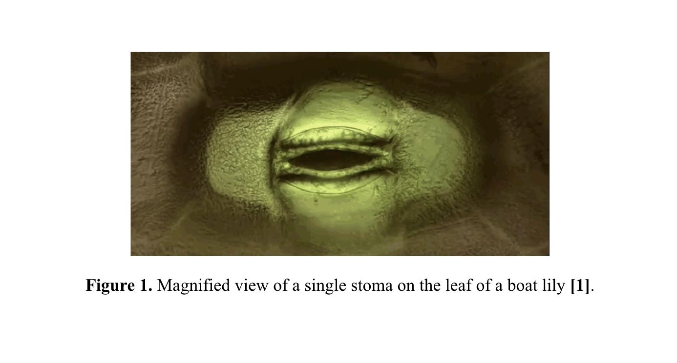
Plants take in carbon dioxide and water through two dif systems. They absorb water their root system and carbon through their leaves. On undersides of plants’ leaves other places depending on organism) are thousands of (Fig. 1), which open to allow When stomata are open, the inside the plant is exposed and water released into the environment. order to prevent the plant from drying out, open way

1 Corresponding author: jmenschik@thegraysonschool.org Department of Science, Class of 2026, The Grayson School, Radnor PA. Menschik, Scientific

balance between intake of CO2 and water [1]. Certain protein kinases, specifically MPK4/12 and HT1, help sense carbon dioxide in the environment and signal the stomata [2].

In 1804, research by Théodore de Saussure on pea plants exposed to high amounts of carbon dioxide indicated that elevated levels of carbon dioxide in the plant’s environment increased size and yield [10]. Carbon dioxide levels can be increased in the air, or alternatively by adding CO2 to the water. Several research papers have been published showing the results of the addition of carbon dioxide to water, creating carbonated water (CO2(g) + H2O(l) → H2CO3(aq)). The reaction for carbonated water creates carbonic acid, which shifts the water pH towards the acidic end of the scale. This factor may have effects on plant growth.

In 1980, Nakayama and Bucks experimented with buried trickle irrigation systems as a means of distributing carbonated water. They found a 10-20% increase in the yield of melon, potato, and wheat plants. In 1991, Novero et al. found that when using carbonated irrigation water there was a 16% yield increase in tomato plants. Over the years various experiments have shown that using carbonated water increased yield in plants such as corn, sunflower, sorghum, soybean, cotton, potatoes, and tomatoes. There are, on the other hand, studies showing negative or nonexistent impacts of carbonated water Hartz and Holt, in 1991, reported significant negative effects on the growth of cucumber and tomato plants. Storlie, in 1992 reported that carbonated water had no effect on the growth of pepper [3]

A sample that remains to be tested on is the Wisconsin Plant®, a common experimental plant model chosen for growth cycle. Wisconsin Plants® (B. rapa) were developed in 1987 by Williams, in the Department Plant Pathology at the University Wisconsin-Madison. The were first developed to speed research on the disease resistance cruciferous plants. Through years of breeding, fast plants from a 6-month life cycle 5-week life cycle, making model plant sample for rapid experimentation [9]. Petite Wisconsin Fast Plants are typically 5 to 15 centimeters tall, compared to the standard Wisconsin Fast Plants®, which are on average around 20 cm tall. This scaled down size helps allow the plant to grow to their full height in a smaller apparatus.

The result of a plant having access to carbon dioxide through only its water source, and being deprived of it in its atmosphere is so far unexplored. In this experiment there were four separate groups, raised in different environments. One group was grown in normal conditions, one group was given carbonated water, one group was given carbonated water and an oxygenated environment, and the last group was only given an oxygenated environment. To collect quantitative results, analog-to-digital sensors (Sensirion SCD41) were connected to an Arduino Uno programmed to collect continuous data on CO2 concentration, temperature, and relative humidity. Through these variations and data collection the individual effects of carbonated water on plant samples can be studied more thoroughly, using Petite Wisconsin Fast Plants®, a both convenient and interesting sample.

MATERIALS and METHODS

Growth Apparatus

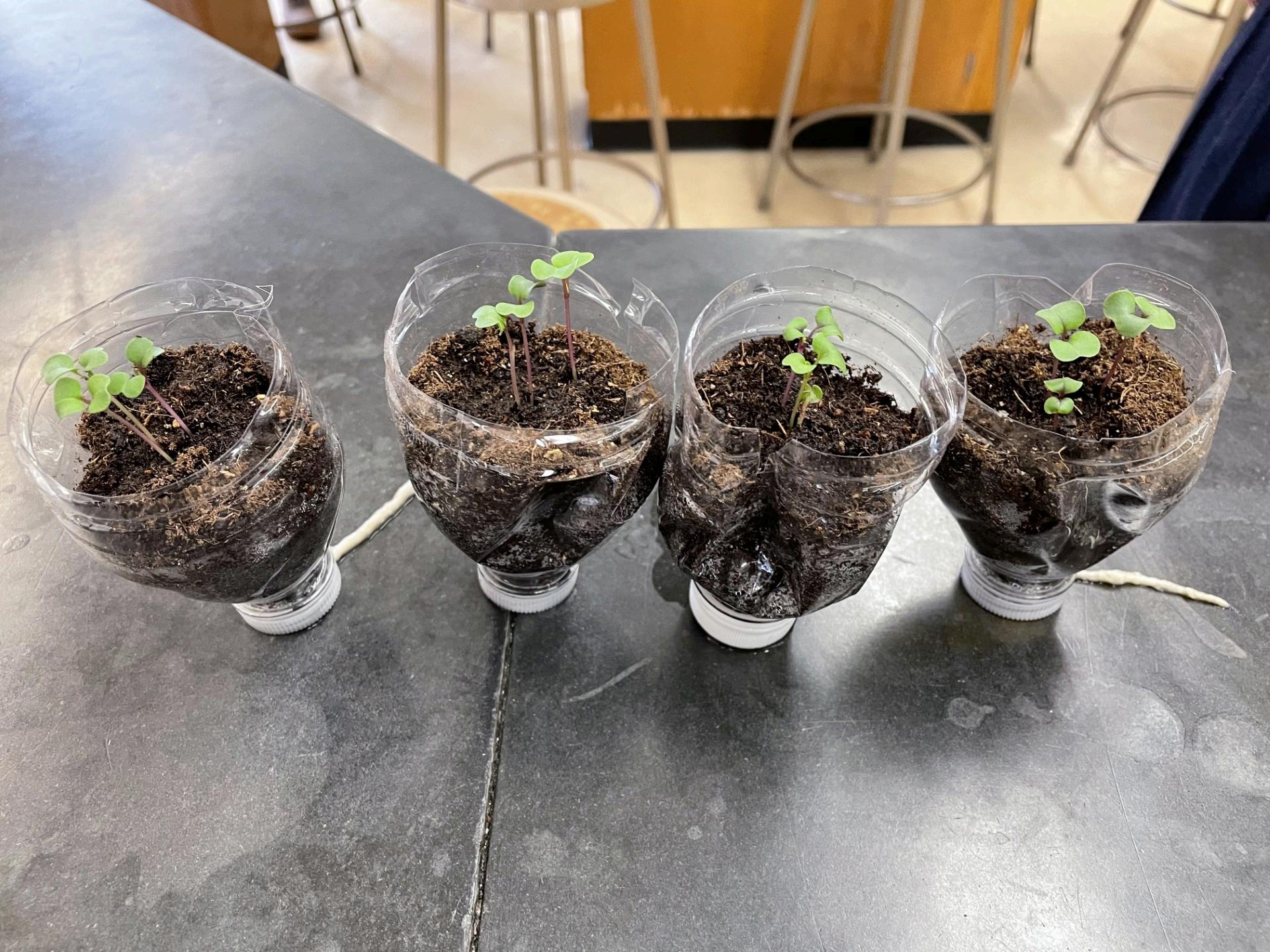
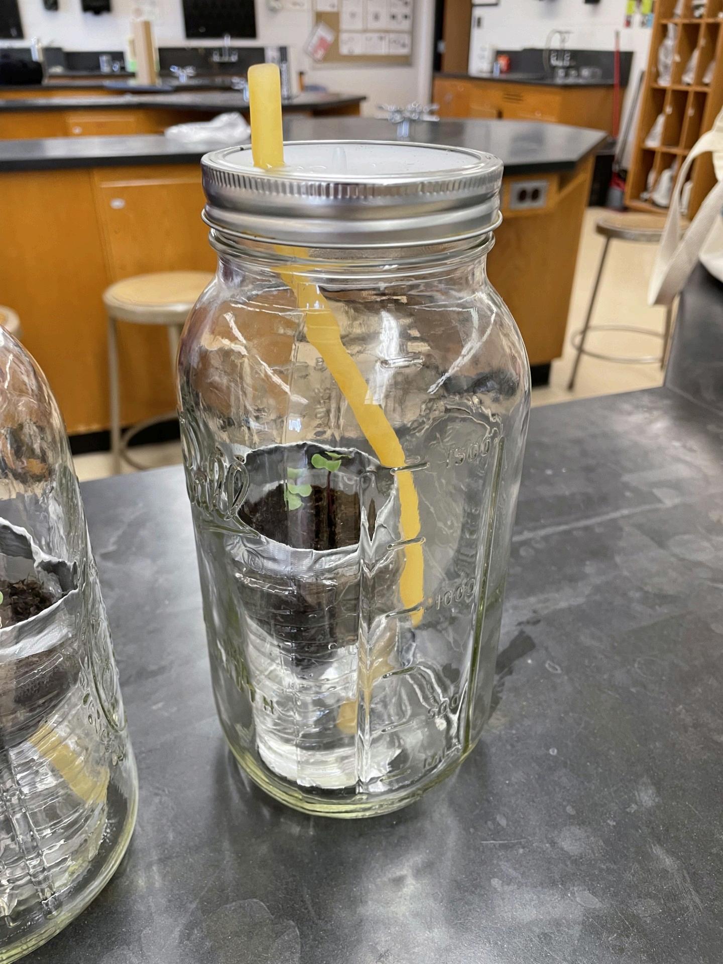
In four separate apparatuses, Petite Wisconsin Fast Plants® (B. rapa) were planted, with three seeds per planter. Wisconsin Fast Plants® require a constantly moist environment, so using an inverted bottle apparatus, the plants were watered through the traditional wick method. The upper container held the soil, the lower container held the water, and an absorbent wick connected the two (Fig. 3). Additionally, Wisconsin Fast Plants require constant light to grow, so all four plants were placed in a standard light box for the entirety of the experiment.

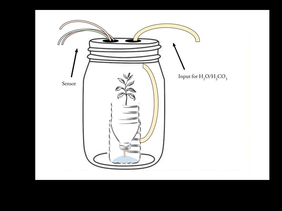
Figur plant, the lower wick connects chamber.

Data Collection

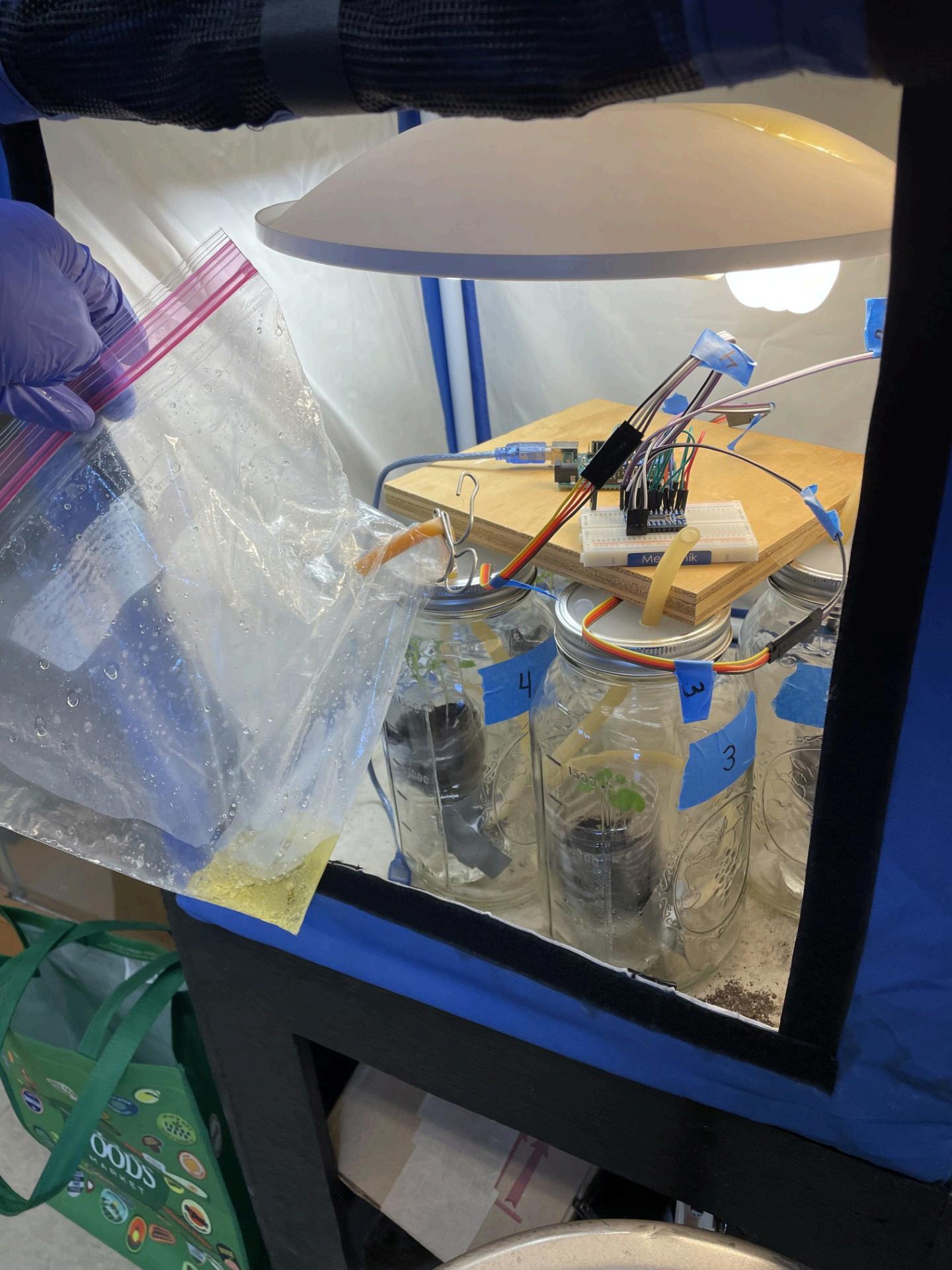
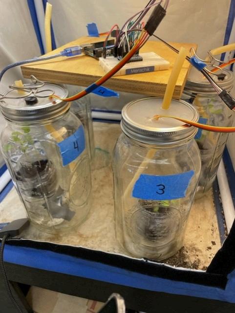
Four identical Sensirion SCD41 sensors were connected to an Arduino Uno using a multiplexer (Texas Instruments TCA9548A) to overcome the limitation of a single analog-to-digital channel on the Uno. The Uno was programmed to collect data on CO2 concentration in parts per million, temperature in Celcius, and relative humidity (Fig. 4). Data was collected every 5 seconds, alternating between the four sensors. The codebase is available at https://github.com/juliak8/sci-inquiry (as referenced in the appendix).

Figure 4. - Wiring diagram schematic connecting the Arduino, multiplexer (TCA9548A) and four SCD41 sensors, one placed in each controlled environment

On the 21st day of the plants’ life cycle the experiment ended and final data was collected. Each plant was measured for height and mass, and then prepared for a Vitamin C titration. For the titration, all three plants from each apparatus were crushed, along with 2mL of dH2O, with a mortar and pestle. A reference solution was created by adding 1.0g of oxalic acid to 100mL of dH2O, and then adding 0.100g of ascorbic acid to that solution. Then the 2,6-Dichloroindophenol solution was made by adding 0.06g of 2,6-Dichloroindophenol to 100mL dH2O. In a reaction plate, three samples (0.5 mL each) of each crushed plant solution were added to a reaction plate, along with three samples of the reference solution. Using a 1mL pipette, the 2,6-Dichloroindophenol solution was dropped into a reference solution plate one drop at a time until the solution turned faintly pink. The number of drops were recorded. This procedure was repeated with each plant sample.

Experimental Procedure

On the thirteenth day of the plants' life cycle, respective variables were added to each growth apparatus. Group 1 continued with normal tap water and the water tube was left open to the air In Group 2, a third hole in the lid of the jar was created, and O2 gas was fed in, while the air left through the open water port. To produce the O2 , KI salt was added to a 1 gallon sealable bag with a small tube. The air was removed from the bag using a syringe attached to the tube. Then using the syringe, 3% H2O2 was added, and O2 gas was produced. After the oxygen filled the jar the new hole was sealed. Then using the water tube the lower chamber of the bottle was filled with carbonated water The carbonated water was produced by reacting NaHCO3 and 5% acetic acid to create CO2 , and then slowly saturating tap water with the carbon dioxide. After filling the water chamber, the tube was sealed with a clamp. In Group 3 the carbonated water procedure was repeated, but no O2 was added to the jar The water tube was left open to the air In Group 4 the O2 procedure was repeated, but the plant continued to be fed standard tap water. A sensor was added to the left valve of each jar, and continually measured CO2 in ppm, relative humidity, and temperature in Celcius.

Table 1. Group variation in water type and gas environment.

Group Water Type Gases

1 Standard (H2O) N2 (78%), O2 (21%)

2 Carbonated (H2CO3) O2 (100% )

3 Carbonated (H2CO3) N2 (78%), O2 (21%)

4 Standard (H2O) O2 (100% )

RESULTS

The results of this experiment remain inconclusive. Group 4 (Mason Jar 4) was intended as a control deprived of carbon dioxide, which would in theory lead to plant deterioration or death, yet Group 4 remained alive and showed a comparable mass and height to the other groups, and even showed a significantly higher CO2 concentration than the other groups throughout the experiment (Fig. 5) (Fig. 6) (Fig. 7). The group that performed the best in mass and size was Group 1, which was grown under normal conditions. The Vitamin C titration procedure proved inconclusive on all plant samples, likely indicating that the ascorbic acid concentration in those samples was too low for detection.

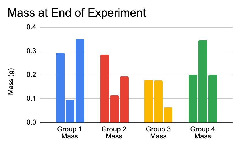
5. - Mass of each plant in each group at the end of the experiment (day 21 of life cycle).

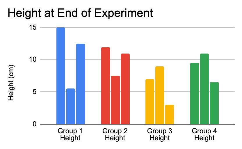
6. - Height of each plant in each group at the end of experiment (day 21 of life cycle).

Figure

Figure

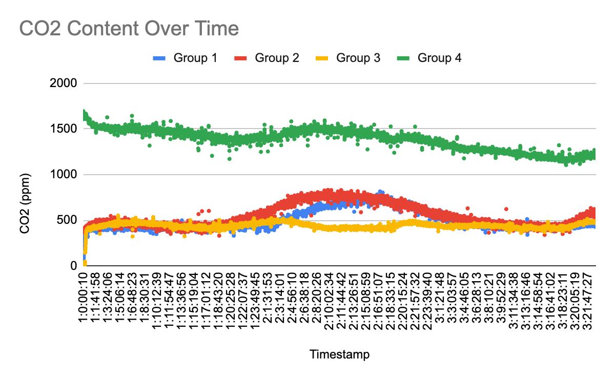
Figure 7. - Carbon dioxide concentration inside each apparatus, day 19-21 of life cycle, measured in parts per million. Timestamp measured in DAY:HOUR:MINUTE:SECOND since data collection began.

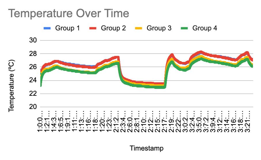
Figure 8. - Temperature inside each apparatus, day 19-21 of life cycle, measured in Celsius.

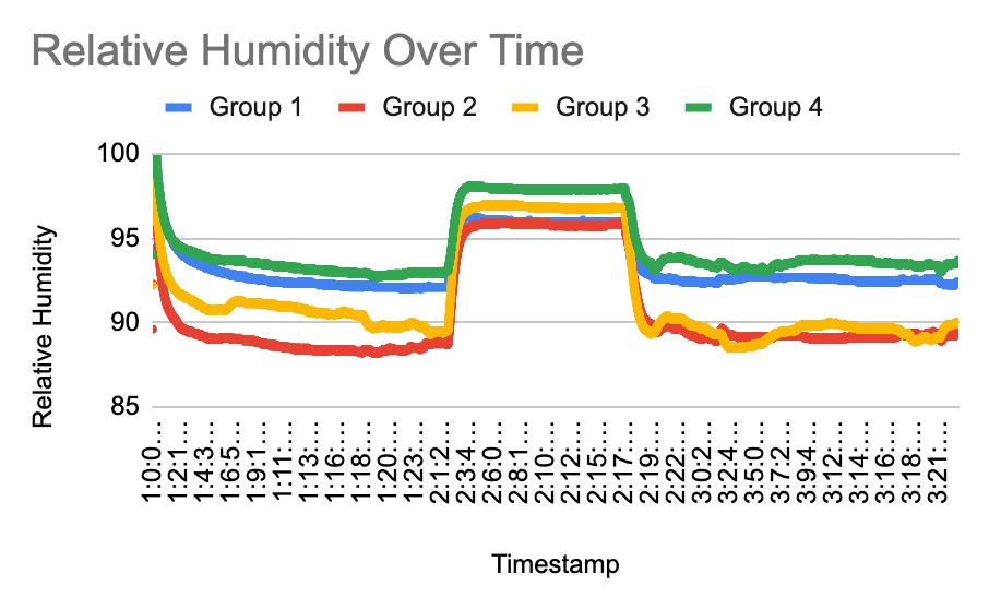
Figure 9. - Relative humidity inside each apparatus, day 19-21 of life cycle.

DISCUSSION

As previously mentioned, failure of the control indicates the data collected is inconclusive. This could be due to any number of factors. One possible conclusion is that an insufficient amount of O2 was added to the mason jar. Another conclusion is a failure in the sealing method, leading to oxygen slowly escaping while air flowed in. Sensor data collection was also stalled at the beginning of the experiment due to equipment malfunction. The author intends to rerun the experiment under more controlled conditions and revise her conclusions.

ACKNOWLEDGEMENTS

We would like to thank Flinn Scientific and University of Wisconsin-Madison for providing the materials used during this experiment. We thank E. Menschik, B. Muaddi, T Nevins-Klein, N. Freidenreich, M. Sizer, and classmates for their feedback on analysis and interpretation. The scientific results and conclusions and any views or opinions expressed herein are those of the author and do not necessarily reflect the views and policies of the Grayson School, Delaware County, or the US government and its agencies.

Funding: This experiment was supported by the Department of Science, The Grayson School. Competing interests: The authors declare no competing interests. Menschik, Scientific Transactions of

REFERENCES

1. Dashoff, Jared “Scientists discover mechanism plants use to control 'mouths '” NSF, 7 December 2022, https://www nsf gov/science-matters/scientists-discover-mechanism-plants-use-control Accessed 28 February 2025.

2. Takahashi, Yohei et al “Stomatal CO2/bicarbonate sensor consists of two interacting protein kinases, Raf-like HT1 and non-kinase-activity requiring MPK12/MPK4 ” Science, ScienceAdvances, 7 December 2022, https://www.science.org/doi/10.1126/sciadv.abq6161. Accessed 28 February 2025.

3. Alvino, A , et al “Physiological response of Gladiolus to carbonated water application under two water regimes ” Advances in Horticultural Science, vol 12, no 3, 1998, pp 145-152, https://www-jstor-org proxy library upenn edu/stable/pdf/42883202 pdf?refreqid=fastly-default%3A62e053 dbb247ca9636fbdfbf44a95ca8&ab segments=&initiator=&acceptTC=1.

4. “Potassium Iodide SDS (Safety Data Sheet) ” Flinn Scientific, 21 March 2014, https://www flinnsci com/sds 638-potassium-iodide/sds 638/ Accessed 28 February 2025

5. “Three mistakes to avoid for growing healthy Fast Plants.” Wisconsin Fast Plants, https://fastplants org/2018/10/17/growing-healthy-fast-plants/ Accessed 28 February 2025

6. “Teaching and Learning Through the Wisconsin Fast Plants® Life Cycle ” Wisconsin Fast Plants, 13 March 2017, https://fastplants.org/2017/03/13/life-cycle-fast-plants/. Accessed 28 February 2025.

7. Flinn Scientific, Inc “Oxalic Acid Dihydrate Safety Data Sheet (SDS) ” Flinn Scientific, 21 March 2014, https://www flinnsci com/sds 571-oxalic-acid-dihydrate/sds 571/ Accessed 4 March 2025

8. Flinn Scientific Inc. “2 6-Dichloroindophenol Safety Data Sheet (SDS).” Flinn Scientific, 16 January 2014, https://www.flinnsci.com/sds 303-2-6-dichloroindophenol/sds 303/. Accessed 4 March 2025.

9. University of Wisconsin-Madison “Origin - Wisconsin Fast Plants® ” Fast Plants, https://fastplants org/origin/ Accessed 6 May 2025

10. de Saussure, Théod. “Recherches chimiques sur la végétation.” Biodiversity Heritage Library, 1804, https://www biodiversitylibrary org/item/55536#page/2/mode/1up

APPENDIX

All code and schematics used for this experiment can be found at the following GitHub Repository: https://github.com/juliak8/sci-inquiry

Environmental stresses emulating the Great Oxidation Event as drivers of multicellular evolution

Jacob Lee1

ABSTRACT

The transition from unicellular to autonomous multicellular life was a major evolutionary milestone, yet the mechanisms behind this transition remain poorly understood. Multicellularity evolved independently in multiple eukaryotic lineages, many coinciding with the Great Oxidation Event (GOE), when photosynthetic cyanobacteria oxygenated the Archean atmosphere. This experiment explores this link by exposing Saccharomyces cerevisiae to environmental conditions simulating GOE-associated chemical stressors. After 3 weeks, aggregation was observed in response to both metal toxicity and oxidative stress. Metal exposure induced flocculation, a stress response, while high oxidative stress led to post-division retention—suggesting heritable multicellular behavior, though genetic confirmation is pending. These findings lend preliminary support to the hypothesis that the GOE fostered conditions that actively promoted the emergence of multicellular life.

INTRODUCTION

From single cells to the various eukaryotic organisms known today, the astonishing complexity of life has perplexed scientists for years. In 1953, Nobel laureate Harold Urey and then-graduate student Stanley Miller ushered in a new era of experimental research into the origin of life with the famous Miller-Urey experiment (1). By emulating the conditions of early Earth, they demonstrated naturalistic origins for the building blocks of life from inorganic precursors. Since then, naturalistic explanations for abiogenesis2 and the endosymbiotic3 origins of eukaryotes have advanced significantly (2) (3). However, the mechanisms driving the evolution of multicellularity remain unclear.

The transition to multicellularity was not a single, all-encompassing event, but rather unique to different types of organisms, emerging over 25 times independently across the phylogenetic tree (4). Still, researchers agree on a few common evolutionary advantages that facilitated it. Namely, protection against predation (5) (6); more efficient chemotaxis4 and mobility, leading to improved resource acquisition (7); and tolerance to abiotic stressors (8). These advantages became critical during major environmental upheavals. One such upheaval was the Great Oxidation Event (GOE)—a period of dramatic change in early Earth’s history

1 Corresponding Author.

2 The origin of life on Earth from non-living matter through natural processes

3 The original internalization of prokaryotes by an ancestral eukaryotic cell.

4 The directed movement of a cell or organism in response to a chemical stimulus

contemporaneous with the emergence of multicellularity, creating selective abiotic pressures that may have favored multicellular traits.

Between 2.3 and 2.5 billion years ago, Earth's atmosphere—initially anoxic and rich in nitrogen (N2), carbon dioxide (CO2), and methane (CH4)—began to oxygenate due to photosynthetic cyanobacteria, triggering the 200-million-year-long GOE (9). Oxygen accumulated in Earth’s atmosphere and surface waters causing chemical changes that acted as selective pressure for oxidative stress tolerance. The once anoxic, Fe2+ rich oceans oxidized, producing Fe3+ as a precipitate, and the presence of oxygen triggered the formation of hydroxyl radicals, H2O2, and other reactive oxygen species (ROS), which impaired the function of biomolecules (10). ROS such as hydrogen peroxide and hydroxyl radicals can damage DNA, proteins, and lipids, leading to heritable mutations as well as reversible physiological responses. In microorganisms, oxidative stress has been shown to increase mutation rates (11), potentially accelerating adaptive evolution under environmental pressure.

Previous studies have demonstrated that selective environmental pressures such as gravity or predation can encourage multicellularity in some single-celled eukaryotes (6) (12) Notably, in a 2012 experiment, Ratcliff et al. (12) repeatedly selected for fast-settling yeast, inducing the evolution of clonal, multicellular clusters coined “snowflake yeast.” These clusters exhibited key, heritable features of multicellularity, including cell-to-cell adhesion, and programmed cell death. Genomic analyses revealed mutations in genes relating to post-mitotic cell separation and apoptosis, suggesting a genetic basis for the transition.

In that model, multicellularity emerged due to physical selection favoring fast sedimentation rather than environmental stress. In contrast, this study investigates whether multicellular traits can be induced by oxidative and metal stressors associated with the Great Oxidation Event (GOE). By simulating chemical hostility, this experiment aims to determine if external stress can drive yeast toward multicellularity without the same level of selection for sedimentation.

S. cerevisiae, an ideal model organism due to its short generation time, conserved eukaryotic processes, and phenotypically observable evolutionary changes (13) (14), were used in 5 separate, easily reproducible trials (Table 1). This study hypothesizes that oxidative stress and metal toxicity will accelerate multicellular traits in S. cerevisiae, suggesting that environmental hostility during the GOE did not just coincide with, but actively facilitated multicellular evolution.

Table 1. Experimental Setup of Stressor Trials.

Each 10 mL culture contains S. cerevisiae and different combinations of stressors to simulate Great Oxidation Event-like environments.

Trial Stressor concentrations

Control N/A N/A N/A

Metal toxicity (ROS enhancers)

100 µM FeCl3·6H2O and 25 µM CuSO4·5H2O

Sub-lethal cytotoxicity and weak oxidative stress

Oxidative stress

100µM H2O2

Metal toxicity and oxidative stress

100 µM FeCl3·6H2O, 25 µM CuSO4·5H2O, and 100µM H2O2

Strong oxidative stress

The oxidation of Fe²⁺ to Fe³⁺ was accompanied by the oxidation of copper minerals, increasing the availability of Cu²⁺ in surface environments. (15)

UV irradiation and radiolysis of water generated H2O2 through the formation and recombination of reactive radicals (16)

Sub-lethal cytotoxicity and strong oxidative stress

See above (15) (16)

MATERIALS and METHODS

Yeast was initially aliquoted at 1 mg per 10 mL into five separate test tubes. Each 10 mL solution contained 0.2 g sucrose and 0.2 g peptone in distilled water as the nutrient medium. The concentrations of metal stressors and oxidants were chosen to be sub-lethal (17) (18) (19) yet sufficient to induce physiological stress and selective pressure (see Table 1 for details).

Selection and transfer

Transfers were done approximately every 24 hours (± 90-120 mins) using passive settling selection where 1 mL was taken from test tubes and allowed to settle for 30 minutes. The bottom 100 µL were then transferred into a new test tube with the same concentrations of nutrients and stressors. These daily transfers served two purposes: (1) to replenish nutrients and potentially degraded stressors, and (2) to mimic genetic drift by creating a population bottleneck, potentially accelerating adaptive responses (20). Passive selection was used instead of centrifugation, as strong sedimentation selection alone can induce multicellularity in S. cerevisiae, (12) potentially confounding results by making it a facultative response rather than one driven by environmental stressors.

Slide preparation and microscopy

To prepare slides for observation, the 1 mL yeast sample from the transfer procedure was subject to mild centrifugation to break apart loose clumps, potentially allowing for clearer distinction between true multicellular clusters and transient flocculation. A 10 µL aliquot from the pellet was stained with 1 µL methylene blue and mounted on a slide. To prevent dehydration during observation, a thin ring of clear nail polish containing ethyl acetate, nitrocellulose, butyl acetate, and camphor was applied around the coverslip. Slides were imaged using oil immersion microscopy at 1000x magnification.

Consistent with criteria from prior studies (13), key indicators included: (1) persistence of clusters after mild centrifugation; (2) geometric growth patterns (13); and (3) apparent cellular adhesion (as opposed to random collision which is determined primarily by the presence of a complete cell wall). While Ratcliff et al. confirmed multicellularity using gene sequencing and assays for apoptosis, this study used morphological proxies observed via light microscopy to identify early multicellular structures.

RESULTS

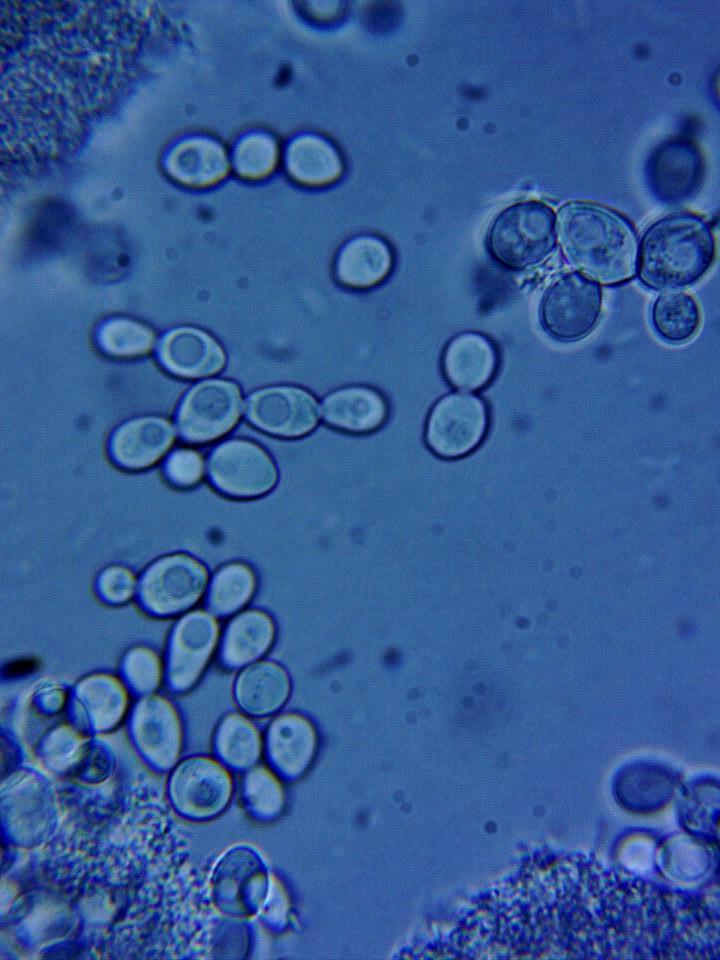
After 2 weeks of selection, some aggregation was observed in S. cerevisiae exposed to metal toxicity. Clear stress responses were observed in those exposed to oxidative stress with clumps of cells, some without complete cell walls indicating potential failed post-mitotic separation, a step towards early multicellularity (Figure 1).

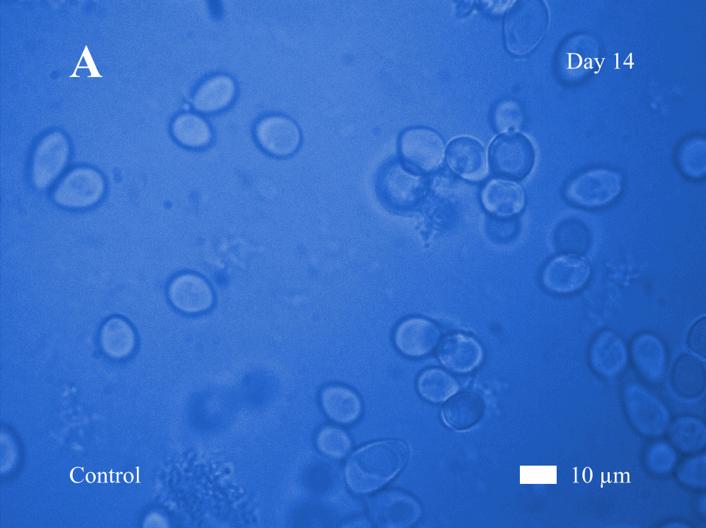
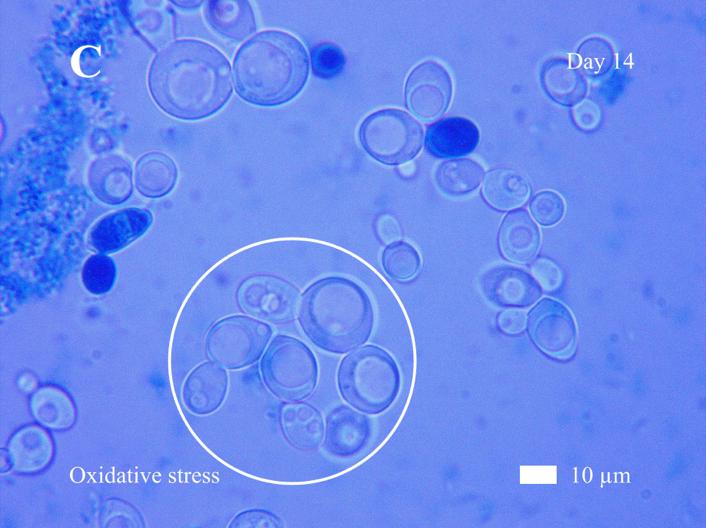
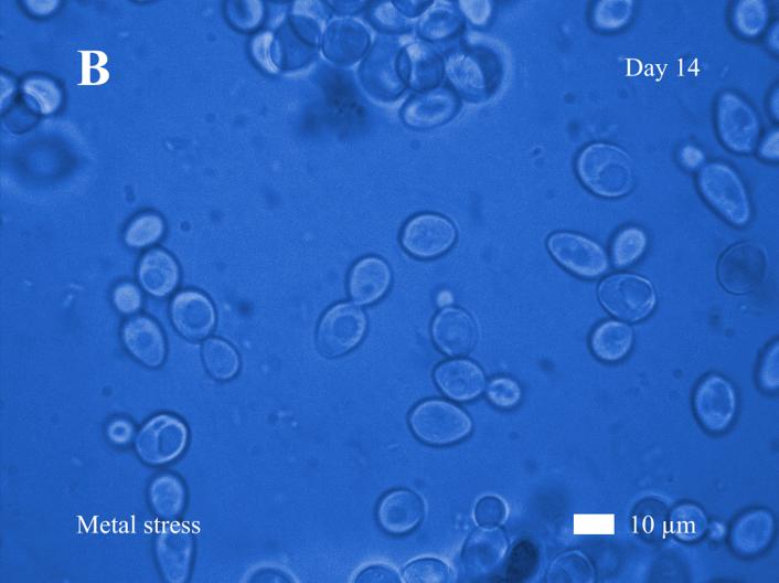
After 3 weeks of selection, more clear morphological changes were observed in S. cerevisiae across the various stress conditions (Figure 2). Microscopy revealed patterns of cellular aggregation consistent with the expected responses to oxidative and metal-induced stress. Cells exposed to metal toxicity (100 µM Fe3+ and 25 µM Cu2+) aggregated into large flocculation-like masses (Figure 2). However, individual cell boundaries remained distinct, and the aggregation was visibly distinct from the uniformity of clonal clusters. This morphology is consistent with what is known about flocculation; it is a reversible, stress-induced adhesion response (21) Yeast exposed to oxidative stress (100 µM hydrogen peroxide) also formed aggregates but appeared to have remained connected after division in small, clonal clusters

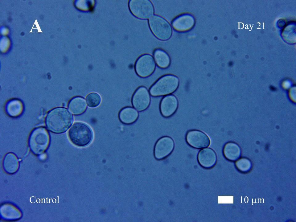
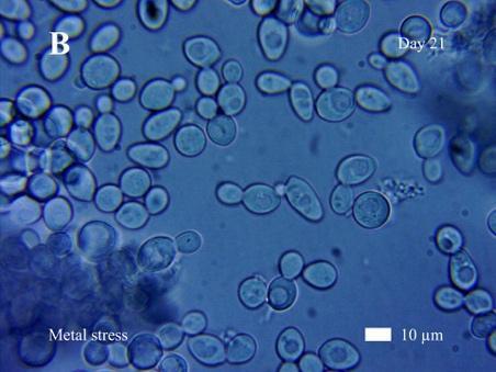
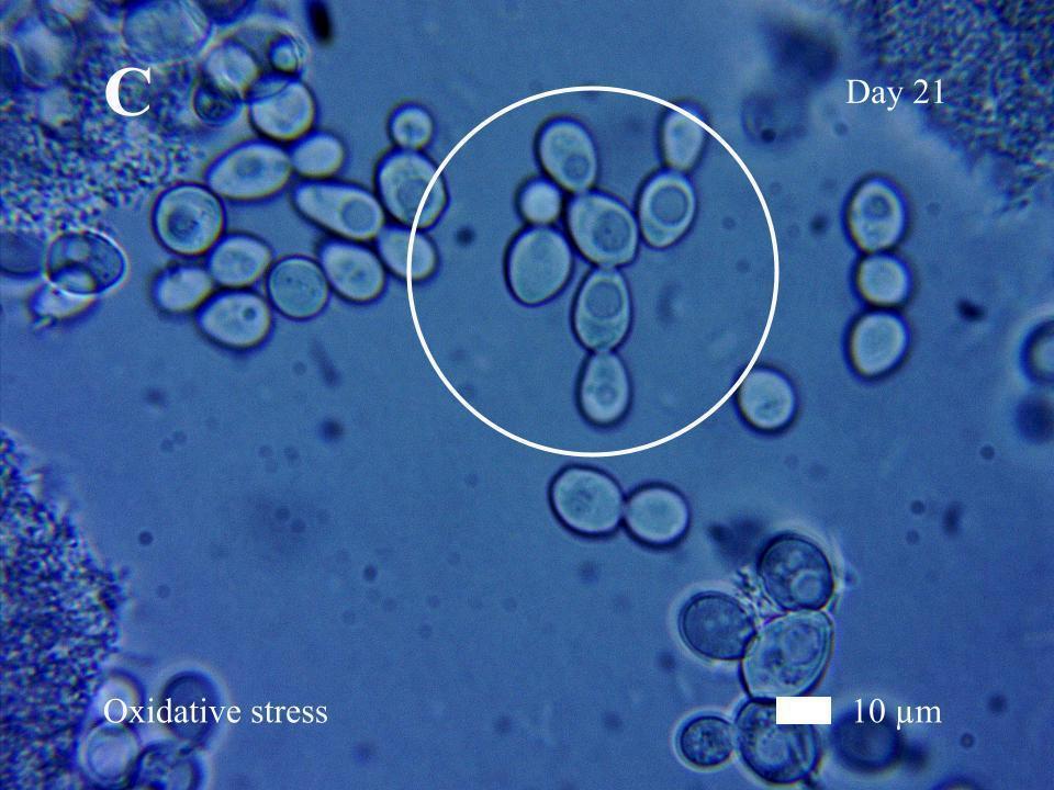
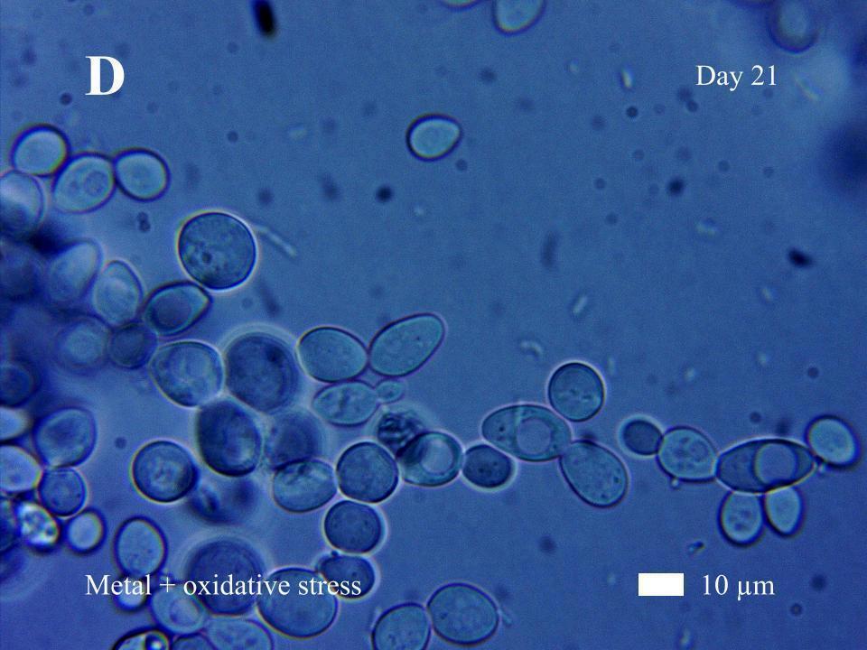
Figure 2. This post-division adhesion suggests possible suppression of daughter cell separation, a behavior previously associated with early multicellular development (13).

Groups under oxidative stress settled faster through liquid media by the end of the 3-week experiment (Figure 3). Settling speed is often a good indicator of aggregation, as larger clumps of cells settle more rapidly than smaller individual cells. These observations, while preliminary, are consistent with the evolution of increased cell-cell cohesion under oxidative stress.

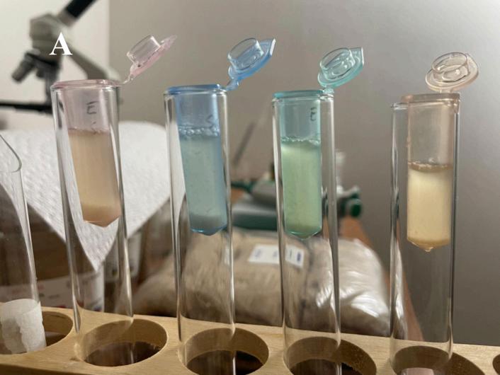
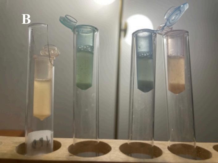
Table 2. Comparative morphology

Summary of morphological observations in S. cerevisiae over time after exposure to different GOE-like stress conditions

Trial Morphology (after 2 weeks) Morphology (after 3 weeks) Hypothesized mechanism

Control Single cells or normal budding, no clustering

Metal toxicity

Oxidative stress

Oxidative and metal induced stress

Single cells or normal budding, some clustering

Small, possibly clonal aggregates

N/A

Single cells or normal budding, no clustering

No stress so no aggregation

Non-clonal aggregates Flocculation and a phenotypic stress response

Smaller, uniform clusters of seemingly clonally linked cells

Post-division retention from genetic mutation

Dense, non-clonal aggregates Flocculation and a phenotypic response to acute stress

DISCUSSION

This experiment investigated how environmental stressors simulating the conditions of the GOE influence the development of multicellular traits in Saccharomyces cerevisiae. After three weeks, yeast exposed to oxidative stress (H2O2 alone) formed clusters suggestive of clonal multicellularity, whereas metal-exposed trials tended to show flocculation behavior indicative of stress-induced aggregation.

These findings support the hypothesis that oxidative stress may have acted as a selective driver of multicellularity during the GOE. As oxygen accumulated, organisms likely faced the risk of oxidative damage. The post-division adhesion of daughter to mother cells could have been an adaptive strategy to aid in stress tolerance. Mechanistically, post-division adhesion hints at a mutation in regulatory genes like ACE2, which governs mitotic separation (13).

In addition to causing physiological stress, ROS can directly induce mutations by damaging DNA bases and breaking strands (11) Over time, this can lead to adaptive genetic changes in stress-response or the critical cytokinesis genes such as ACE2 or AMN1. In this context, the observed post-division retention may indicate more than phenotypic plasticity; it

Lee, Scientific Transactions of the Grayson Society, May 2025

could reflect emerging genotypic adaptations to oxidative environments—linking stress directly to evolutionary innovation.

While these observations align with past studies showing that sedimentation selection or predation pressure can induce multicellularity (6) (12), this experiment is novel in its use of geochemical stress as a sole driver as well as early Earth analog and offers experimental support for the hypothesis that the conditions of the GOE not only coincided with, but actively catalyzed the evolution of multicellularity.

Several shortcomings in the experimental setup and execution must be acknowledged. The setup did not control for temperature and was unable to recreate the myriad of substances that would have been present in the ocean during the GOE with distilled water as the only solvent which compromises on the fidelity of the analog, oversimplifying the chemical complexity of GOE-era oceans. Moreover, the results here are from one group, as the various trials were not run with replicates compromising their generalizability The lack of significant numerical data limits the extrapolatory potential of these conclusions; future work should focus on acquiring more data points to get quantitative results.

While this experiment highlights a morphological shift toward multicellularity under GOE-like stressors, it remains uncertain whether these changes reflect true evolutionary adaptation or plastic physiological responses. A key next step would be to isolate evolved lineages and conduct whole-genome sequencing to identify recurrent mutations—especially in genes like ACE2 or AMN1, known to mediate post-mitotic separation (13) (22) Ultimately, this model opens new avenues to explore how geochemical phenomena may have shaped the earliest multicellular life.

ACKNOWLEDGMENTS

The author would like to thank M. Sizer for his guidance developing procedures and helping plan the experiment.

The scientific results and conclusions and any views or opinions expressed herein are those of the author and do not necessarily reflect the views and policies of The Grayson School, Delaware County, or the US government and its agencies.

Funding: This experiment was supported by the Department of Science, The Grayson School. Competing interests: The author declares no competing interests.

REFERENCES

[1] Stanley L. Miller, A Production of Amino Acids Under Possible Primitive Earth Conditions. Science 117, 528-529 (1953) DOI: 10 1126/science 117 3046 528

[2] Pross, Addy, and Robert Pascal “The origin of life: what we know, what we can know and what we will never know.” Open biology vol. 3,3 120190. 6 Mar. 2013, doi:10.1098/rsob.120190

[3] Archibald, John M “Endosymbiosis and Eukaryotic Cell Evolution ” Current biology : CB vol 25,19 (2015): R911-21 doi:10 1016/j cub 2015 07 055

[4] Grosberg RK, Strathmann R. 2007. The evolution of multicellularity: a minor major transition? Annual Review of Ecology, Evolution, and Systematics 38, 621–654.

Lee, Scientific Transactions of the Grayson Society, May 2025

[5] Herron, Matthew D et al “De novo origins of multicellularity in response to predation ” Scientific reports vol 9,1 2328 20 Feb 2019, doi:10 1038/s41598-019-39558-8

[6] Fisher, R. M., Bell, T., & West, S. A. (2016). Multicellular group formation in response to predators in the alga Chlorella vulgaris Journal of Evolutionary Biology, 29(3), 551–559 https://doi org/10 1111/jeb 12804

[7] Enrico Sandro Colizzi, Renske MA Vroomans, Roeland MH Merks (2020) Evolution of multicellularity by collective integration of spatial information eLife 9:e56349

[8] H. Isaksson, P. Lind, & E. Libby, Adaptive evolutionary trajectories in complexity: Transitions between unicellularity and facultative differentiated multicellularity, Proc Natl Acad Sci U S A 122 (4) e2411692122, https://doi org/10 1073/pnas 2411692122 (2025)

[9] Catling, D. C., & Zahnle, K. J. (2020). The Archean atmosphere. Science Advances, 6(9), eaax1420. https://doi org/10 1126/sciadv aax1420

[10] Shields, Hazel J et al “Beneficial and Detrimental Effects of Reactive Oxygen Species on Lifespan: A Comprehensive Review of Comparative and Experimental Studies.” Frontiers in cell and developmental biology vol. 9 628157 11 Feb 2021, doi:10 3389/fcell 2021 628157

[11] Afzal, Sheryar et al “From imbalance to impairment: the central role of reactive oxygen species in oxidative stress-induced disorders and therapeutic exploration.” Frontiers in pharmacology vol. 14 1269581. 18 Oct. 2023, doi:10.3389/fphar.2023.1269581

[12] W C Ratcliff, R F Denison, M Borrello, & M Travisano, Experimental evolution of multicellularity, Proc Natl Acad Sci U S A 109 (5) 1595-1600, https://doi org/10 1073/pnas 1115323109 (201)

[13] Ratcliff, W. C., Fankhauser, J. D., Rogers, D. W., Greig, D., & Travisano, M. (2015). Origins of multicellular evolvability in snowflake yeast Nature Communications, 6, 6102 https://doi org/10 1038/ncomms7102

[14] Botstein D, Fink GR Yeast: an experimental organism for 21st Century biology Genetics 2011 Nov;189(3):695-704. doi: 10.1534/genetics.111.130765. PMID: 22084421; PMCID: PMC3213361.

[15] Willem H Koppenol, Helmut Sies, Was hydrogen peroxide present before the arrival of oxygenic photosynthesis? The important role of iron(II) in the Archean ocean, Redox Biology, Volume 69, 2024, 103012, ISSN 2213-2317, https://doi.org/10.1016/j.redox.2023.103012

[16] Chi Fru, E , Rodríguez, N P , Partin, C A , Lalonde, S V , Andersson, P , Weiss, D J , El Albani, A , Rodushkin, I , & Konhauser, K O (2016) Cu isotopes in marine black shales record the Great Oxidation Event Proceedings of the National Academy of Sciences, 113(18), 4941–4946. https://doi.org/10.1073/pnas.1523544113

[17] Collinson, L P, and I W Dawes. “Inducibility of the response of yeast cells to peroxide stress.” Journal of general microbiology vol 138,2 (1992): 329-335 doi:10 1099/00221287-138-2-329

[18] Vasylkovska, Ruslana & Burdyliuk, Nadia & Semchyshyn, Halyna (2015) Involvement of Catalase in Saccharomyces Cerevisiae Hormetic Response to Hydrogen Peroxide. Journal of Vasyl Stefanyk Precarpathian National University 2 10 15330/jpnu 2 1 107-114

[19] Eduardo V Soares, Kristel Hebbelinck, and Helena MVM Soares 2003 Toxic effects caused by heavy metals in the yeast Saccharomyces cerevisiae: a comparative study. Canadian Journal of Microbiology. 49(5): 336-343. https://doi org/10 1139/w03-044

[20] Izutsu, Minako, et al “Effects of Periodic Bottlenecks on the Dynamics of Adaptive Evolution in Microbial Populations.” Microbiologyresearch.Org, Microbiology Society, 18 Sept. 2024, www.microbiologyresearch.org/content/journal/micro/10.1099/mic.0.001494.

[21] Ildar Nisamedtinov, George G Lindsey, Robert Karreman, Kerti Orumets, Mariane Koplimaa, Kaspar Kevvai, Toomas Paalme, The response of the yeast Saccharomyces cerevisiae to sudden vs gradual changes in environmental stress monitored by expression of the stress response protein Hsp12p, FEMS Yeast Research, Volume 8, Issue 6, September 2008, Pages 829–838, https://doi org/10 1111/j 1567-1364 2008 00391 x

[22] Fang O, Hu X, Wang L, Jiang N, Yang J, Li B, Luo Z Amn1 governs post-mitotic cell separation in Saccharomyces cerevisiae. PLoS Genet. 2018 Oct 1;14(10):e1007691. doi: 10.1371/journal.pgen.1007691. PMID: 30273335; PMCID: PMC6181423

Lee, Scientific Transactions of the Grayson Society, May 2025

Examination of wood ash samples to determine the presence of metal cations Fe3+, Mn4+, K+, Na+, and Ca2+

Jack Hafner1

ABSTRACT

Thirteen elements, specifically B, Zn, Fe, Mn, Cu, Cl, Mo, N, P, Ca, K, Na, and Mg, are considered macronutrients or micronutrients, and they are vital for plant growth and development. In this study, five experiments will be performed to test wood ash for the presence of the metal cations Fe3+, Mn4+, K+, Na+, and Ca2+—all of these being vital nutrients for trees. The pH of the ash will also be measured since many of the soluble compounds in wood ash are known to be alkaline.

INTRODUCTION

Dry wood obtained from trees is composed of about 50% carbon, 44% oxygen, 6% hydrogen2(1), and trace amounts of other elements, including boron, zinc, iron, manganese, copper, chlorine, and molybdenum (2). These seven elements, defined as “micronutrients,” are absorbed from the soil through the tree’s roots. They take up less than 1% of the tree’s mass, but play major roles in maintaining its health and are involved in critical enzymatic reactions such as photosynthesis and respiration (3). Each of these micronutrients has its own unique role; iron synthesizes chlorophyll, manganese works with enzymes to catalyze important reactions, boron supports cell walls and membranes, zinc supports gene expression, copper assists photosynthesis and respiration, molybdenum performs metabolism of atmospheric nitrogen, and chlorine supports osmosis (4).

Trees also require other elements, known as “macronutrients,” for growth and development. The primary macronutrients are nitrogen, which is instrumental in energy metabolism and protein synthesis, phosphorus, which transports and stores energy, forms organic compounds, and stimulates root growth, and potassium, which regulates water and transports reserve substances. The secondary macronutrients are calcium, which stabilizes the cell wall and helps cells grow, magnesium, which constitutes the chlorophyll molecule’s core, and sulfur, which helps form chlorophyll and increases plant defenses (5). It is vital for the health of all plants, trees included, that the aforementioned nutrients are present. Deficiencies in these nutrients can cause effects such as chlorosis—an abnormal loss of green color—stunted growth, and even the death of the plant (4,5). Wood ash, which contains approximately 6-10% of the burnt wood’s mass, is composed of a myriad of minerals and salts, which includes the elements this study is testing for, but also potentially some harmful heavy metals including lead, cadmium,

1 Corresponding author, <jhafner@thegraysonschool org>

2 These values are rounded up

thallium, thorium, uranium, and mercury. This experiment is testing solely for the presence of certain vital nutrients, but similar experiments can be conducted to test for these harmful metals. The ash is obtained through combustion of wood, and it is vital that the wood, ash, and combustion device are all completely dry, as many of the salts this experiment is testing for are soluble in water

In this study, many different methods will be used to test ash obtained from burnt wood for the metal cations Fe3+, Mn4+, K+, Na+, and Ca2+, which are all among these vital nutrients. The presence of these metal cations is expected, but a lack of their presence may be a cause for concern. Statistically, Fe3+, which takes up 5.6% of Earth’s crust, will be the most likely to appear, followed by Ca2+ at 4.3%, Na+ at 2.3%, K+ at 2.0%, and finally Mn4+ at 0.1% (6,7). The presence of metal cations can be influenced by other factors, such as the habitat and type of soil where the tree grew as well as pollution.

MATERIALS AND METHODS

Before any experiments were conducted, an aqueous 0.5% potassium ferrocyanide solution and a saturated sodium bicarbonate solution were made via mixing solid products with distilled water. Wood ash was also placed through a sieve to create a powder used for the experiments and remove unburnt carbon atoms. Some of the powder was placed in distilled water to create an aqueous wood ash solution.

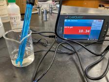
The first experiment was a pH test of the wood ash solution using a LabQuest digital pH meter. After the pH was tested, the solution was left to sit for 24 hours and the pH was tested again.

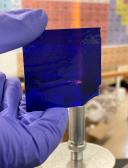
The flame test for metal cations was performed next using a piece of platinum wire that was heated until it started glowing. Then, it was dipped into 10% hydrochloric acid and subsequently into the wood ash. The side of the platinum wire with the wood ash on it was then held into the flame of a butane burner The flame’s color was observed for signs of Na+ and it was observed through a cobalt blue glass to look for signs of K+ Oxidizing melt was then created to test for the presence of manganese. A mixture composed of 0.75 grams of Na2CO3, 0.75 grams of NaNO3, and 0.5 grams of wood ash was created in a mortar and pestle and subsequently placed inside a porcelain crucible that was heated at a gentle flame to prevent NaNO3, an oxidizer, from posing a safety risk. The mixture melted and was left to cool. Once it had cooled, distilled water was added to the crucible and the aqueous contents were added to a test tube. A few drops of a saturated sodium bicarbonate solution were added to reveal the presence of Mn4+ This experiment did not succeed the first time because

unburnt carbon generated smoke and the heat from the butane burner was not enough to form the oxidizing melt, but it did succeed the

second time (Figures 3-4).

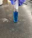
For the fourth experiment, 10% hydrochloric acid was placed in a test tube, as well as some ash which was quickly dissolved. Distilled water was added and the solution was placed through a filter. Then, a few drops of a yellow aqueous potassium ferrocyanide solution were added to create a blue color known as Turnbull’s Blue, revealing the presence of Fe3+

The fifth and final experiment started in the same way as the fourth: by adding 10% hydrochloric acid and some ash to a test tube. Then, distilled water was added and the solution was filtered. The solution was then neutralized with 5% ammonia, taking about 12 drops to do so. After each drop, the pH was measured; the pH meter did not work because of the small amount of solution, so pH strips were used instead. To ensure the presence of Ca2+, a potassium oxalate solution was added to create a white calcium oxalate precipitate.

Potassium oxalate (K2C2O4) and potassium ferrocyanide (C6FeK4N6) were purchased from Flinn Scientific for this study

RESULTS

The wood ash solution’s pH was measured at approximately 11.1. After it was left to sit in a closed container for a day, the pH dropped to 10.34 (Figure 1). This was an unexpected result, as the pH was expected to increase to around 12.

In the second experiment, an orange flame color was visible, confirming the presence of Na+, and a purple flame color was visible through the cobalt blue glass, confirming the presence of K+(Figure 2).

The first attempt at the third experiment failed, with lots of smoke appearing and the solution turning black. On the second attempt, far better results were found, but the solution ultimately tested negative for Mn4+ A positive result should be brown, but the solution remained transparent, indicating that Mn4+ was either not present or present in a very small concentration.

In the fourth experiment, Turnbull’s blue was observed in the sample, indicating the presence of Fe3+(Figure 5). Similarly, in the fifth experiment, a calcium oxalate precipitate was

seen, indicating the presence of Ca2+(Figure 6).

DISCUSSION

Two results obtained through the experiments defied expectations; namely, the negative Mn4+test and the pH test where the pH went down instead of up. The negative Mn4+test could indicate a lack of Mn4+ entirely, but the much more likely outcome is that the Mn4+ concentration was too low to detect. According to the United States Environmental Protection Agency, Mn takes up only about 0.1% of the Earth’s crust, compared to Fe, Ca, Na, and K, which take up 5.6%, 4.3%, 2.3%, and 2.0% respectively.

In the pH test, the solution tested was made of just wood ash and water, yet the pH dropped when it was kept in a closed container for a day. There are many possible causes for this unexpected result. Firstly, it could have dropped due to exposure to sunlight. In a study conducted by Yibeyin Mulualem et al assessing the impact on bottled water of sunlight exposure on a variety of factors, the pH value of bottled water dropped from 7.31 to 7.02 after exposure to sunlight multiple hours a day for a month (8). The pH of the water used in this study dropped from 11.1 to 10.34 in just a day, which is far larger of a difference in a far shorter time. Thus, sunlight exposure is most likely not what caused the drop in pH.

Another possibility to explain this result is that the container was not properly sealed and, because of that, CO2 from the air reacted with the water, forming carbonic acid that reduced the pH. This is the most likely cause, as no significant temperature fluctuations occurred while the solution was being stored.

Additionally, when the first solution for the pH test was made, it had an odd pink color, but the pink color did not appear upon making another solution in the exact same manner Hydrochloric acid was added to the pink solution and it quickly turned clear, indicating that the pink color was caused by accidental cross-contamination with phenolphthalein. The contaminated solution’s pH was not measured and it was disposed of. Another solution was then made.

ACKNOWLEDGEMENTS

I would like to thank Flinn Scientific for providing necessary chemicals, as well as Mr. Sizer for letting me use his lab as well as the materials and tools in it. I would also like to thank The Grayson School for providing funding.

The scientific results and conclusions and any views or opinions expressed herein are those of the author and do not necessarily reflect the views and policies of The Grayson School, Delaware County, or the US government and its agencies.

Funding: This experiment was supported by the Department of Science, The Grayson School.

Competing interests: The author declares no competing interests.

REFERENCES

1. US Department of Agriculture. “Cell Wall Chemistry | US Forest Service Research and Development.” Forest Service Research and Development, 2012, https://research.fs.usda.gov/treesearch/42245.

2. Peryea, Frank. “Managing Micronutrients in Pacific Northwest Orchards.” Washington State University, 1994, revised 2019, https://treefruit.wsu.edu/micronutrients/.

3 Nair, Ajay “Micronutrients Play Large Role in Keeping Plants Healthy ” Iowa State University, 2016, https://www.extension.iastate.edu/news/micronutrients-play-large-role-keeping-pl ants-healthy.

4. Soil Health. “Micronutrients and Their Role in Improving Plant Health Part 1: Intro to Micronutrients.” ST Biologicals, 2023, https://stbiologicals.com/micronutrients-and-their-role-in-improving-plant-health part-1-intro-to-micronutrients/

5 “Macronutrients in plants | AGQ Labs USA ” AGQ Labs USA, 2019, https://www agqlabs us com/macronutrients-in-plants/

6 Town of Rutland, Massachusetts “FAQ: What is manganese and is it dangerous?” https://www rutlandma gov/Faq aspx?QID=118#

7 LePan, Nicholas “Visualizing the Abundance of Elements in the Earth's Crust ” Visual Capitalist, 2021, https://www weforum org/stories/2021/12/abundance-elements-earth-crust/ ’ 8 Mulualem, Yibeyin “Assessing the effect of sunlight exposure on physicochemical properties of bottled water in Addis Ababa, Ethiopia: An experimental observational study ” Science Direct, 2023, https://www sciencedirect com/science/article/pii/S2468227622003593#sec0002

Experimental determination of the photoactive frequencies of silver halides

Tani Nevins-Klein12†

ABSTRACT

The photosensitivity of silver halide crystals has an extraordinary number of applications in photography, general chemistry, and archival media. We provide an introduction to the chemistry of the phenomenon and measure the photochemical properties of three silver halide salts (silver iodide, silver chloride, and silver bromide), including sensitivity to particular frequencies of visible light. While silver bromide and iodide proved too difficult to work with, silver chloride yielded close to expected results, strongly responding to low (violet) frequencies of light.

INTRODUCTION

The first permanent photograph was recorded in 1826 by inventor Joseph Niepce (1). Since that time, photography has blossomed into an immensely important artistic and scientific tool, and a direct application of and breeding ground for new applications of optical physics. Experimentation with the light sensitivity of silver halides – a class of photosensitive salts crucial to almost all photographic techniques is nearly as old, if not older than quantitative chemistry itself. It was known for many centuries that silver salts exhibited a color changing property3, but it was not until the 1720s when German physicist Johann Schulze, conclusively showed that, rather than being thermochromic (sensitive to specific changes in temperature), silver halides were in fact photochromic (sensitive to the radiation of visible light). Schulze placed silver salts in a hot oven and noted that the salts only changed color when exposed to light. In 1770, Swedish scientist Carl Scheele made the important realization that photographic salts underwent their color change by precipitating metallic silver and would “lose” their light sensitivity when exposed to a solution of ammonia, an important precursor to the photographic process.

1 Department of Science, Class of 2025, The Grayson School, Radnor, PA

2† Corresponding author, <tnevins-klein@thegraysonschool.org, tnevinsklein@gmail.com>

3 A historical footnote: a number of sources credit the first discovery of the photosensitivity of silver chloride to a 16th century alchemist named Georg Fabricius. This is false. A 1913 book by German science historian Josef Maria Eder, “Quellenschriften zu den frühesten Anfängen der Photographie bis zum XVIII Jahrhundert ” (trans Sources from the earliest beginnings of photography to the 17th century) writes (machine translation): I have already corrected this erroneous opinion, established in the literature for many decades, that Fabricius was supposed to have known the light sensitivity of silver chloride in 1881. [...] This long-standing uncertainty about the origins of photography is evidently due to the fact that Fabricius's work has become extremely rare and difficult to access. (9)

Nevins-Klein, Scientific Transactions of the Grayson Society, May 2025

Davy and Thomas Wedgwood, attempted to expand on the photographic process by mounting trays of salt inside of camera obscura, a renaissance-era optical device consisting of a large box with a tiny opening in one wall. When placed in a brightly lit environment, an inverted image of the surrounding area is projected onto the opposite wall, ideal for accurately painting landscapes. Davy noted that the image on his silver surface, a proto-photographic film, varied in color significantly based on the environment, though the images were too indistinct to be called photographs. (2)

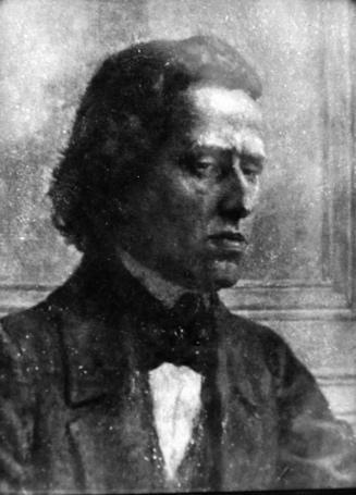
After Joseph Niepce pioneered the first successful photographic process in the mid 1820s, and Louis Daguerre applied Niepce’s optical techniques to a silver plate fumed with halide gasses (Figure 1), the modern photographic process was born. The historical significance of this development cannot be understated. The photographic process, previously inaccessible to all but few specially trained chemists, became a de facto medium for communicating visual information in newsprint, books, posters, and art.

After German-Swiss chemist Christian Schönbein developed a process for its practical production in 1846, nitrocellulose (actually, the sticky, transparent suspension of nitrocellulose in

Nevins-Klein,

ether and alcohol, called collodion) saw wide use as a method of evenly attaching silver halide salts to paper backing, in a process now known as wet-plate collodion photography. Representing significantly shorter exposure times and safer development, the process became immensely popular among professional photographers and hobbyists, despite the requirement for almost immediate development. Many subsequent photographic processes, including modern ones, are essentially variations on this, using a gelatinous medium to adhere and stabilize silver halides to a backing.

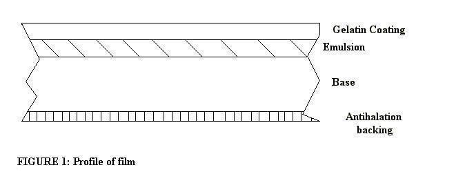
Modern black and white film is composed of four major components: an anti-halation (i.e. light absorbing) backing, an organic base, most commonly PET (polyethylene terephthalate), a silver halide emulsion, and a stabilizing gelatin layer. (3) (Figure 4).

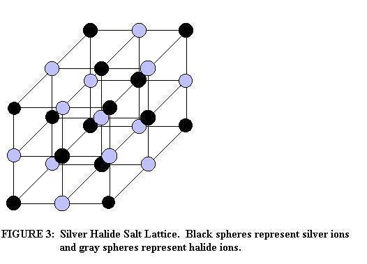
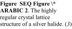
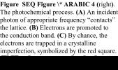
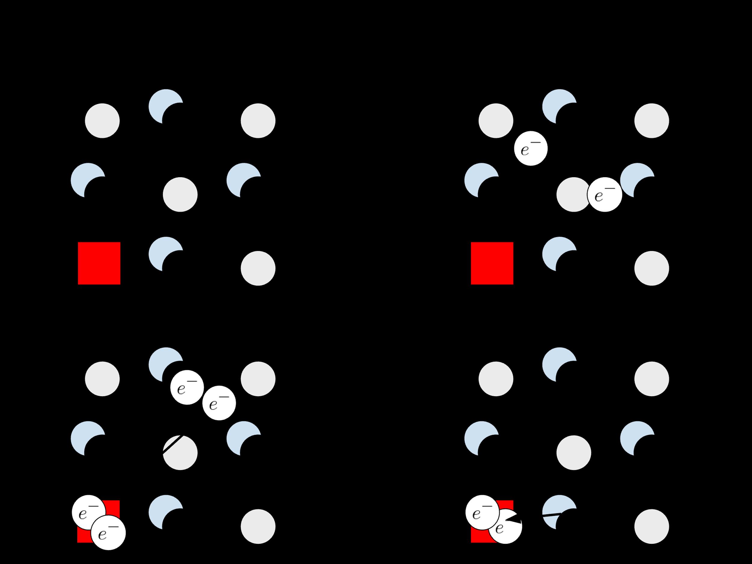
The most significant part of any photographic process is the photochemistry of silver halides. On a photographic plate, the silver and halide ions form into small crystals, called “grains” in the photography world, with a distinctive alternating rectangular lattice structure (Figure 2). Quantum mechanics dictates that the properties of the crystal structure are quantized, and in particular the allowable energies of a particular particle in the lattice are given by discrete bands of energy On contact with a photon, the valence electrons are promoted to a conduction band (i.e. an energy level where they can freely travel the lattice). When slightly perturbed, by either a small structural imperfection or impurity, the free electrons lose energy and settle in a new position, called an electron trap This negatively charged electron trap attracts positively charged silver ions, which form a silver deposit, called the latent image (1)

An important consequence of the quantization of energy is that only very specific energies of photons can activate the photographic process. By Planck’s formula , the � = ℎν energy of a photon is directly proportional to its frequency as a wave. Thus, only particular frequencies of photons can activate the deposition of silver and therefore the photographic process.

The development process reduces the remaining halides while enlarging the metallic silver deposits to be visible (2). This is accomplished in two main chemical steps: the developer, an alkaline mixture, which acts on the silver halides enlarges the deposits of silver ions.

A number of additional chemicals can be added to photographic films to increase or decrease their sensitivity and contrast. Of particular modern interest are activators (or, in the language of condensed matter theory, dopants), impurities added to the silver halide solution with the goal encouraging specific kinds of crystal formation. Activator-based techniques have led to significant advancement in the kinds of high-sensitivity photodetection useful in physics and chemistry. In their 2024 paper “Impact of MO doping on photo-sensing properties for ZnO thin films for advanced photodetection operations,” Shkir et al. investigate the use of doping zinc oxide to create highly effective particle detection systems. (4)

The specific frequencies (energies, by Planck’s formula ) of light that cause this � = ℎν process to occur for a given silver salt, despite their importance for determining exposure times, and understanding the tone composition of a photographic print (as most modern photographic film contains a carefully proportioned mix of the three silver halides), are not easy to calculate

Nevins-Klein, Scientific Transactions of the Grayson Society, May 2025

theoretically. Modern attempts, such as that of R.H. Victoria, make use of advanced quantum mechanical ideas, such as density functional theory (DFT), and still tend to underestimate positions of band gaps – a phenomenon directly related to the reactive frequencies of silver halides (5).

Following prior efforts, we will attempt to experimentally derive the minimum frequencies of light that catalyze the photographic reaction.

Due to the intense light sensitivity of silver halides, we will precipitate our desired silver salt as needed from silver nitrate, which is only slightly photosensitive, at time of experiment. The precipitation is described by the following simple single-replacement reaction common in the study of ionic compounds, where X is either potassium or sodium and Y is one of bromine, iodine, and chlorine (6).

Reaction 1: Precipitation of a silver halide from silver nitrate Here X denotes either sodium or potassium, and Y denotes a halide (either chloride, bromide, or iodide).

Standard literature puts the minimum photoactivation wavelength ranges of each of the salts at violet and ultraviolet for silver chloride ( ), mid-visible blue for silver bromide λ≈400�� ( ), and visible green for silver iodide ( We expect our experimental values λ≈450�� λ≈500��) to err close to this range.

MATERIALS and METHODS

The process of measuring the photosensitivity of the salts occurs in three separate phases: the precipitation of silver halides from silver nitrate, the even distribution of the halides to create a photographic plate, and the exposure of the plate to various frequencies of light. Given the highly photosensitive nature of the experiment, significant portions of the experiment were performed in a makeshift portable darkroom, partially inspired by the plans in Rogge and Bazur ’s 19th Century Photography in a Modern Chemistry Lab. (7) The base of the dark room is a studio lightbox, consisting of four reflective panels joined with flexible semi-transparent black cloth. At the top of a lightbox, a 5W halogen darkroom safe red lightbulb was installed behind a diffusion layer. Over the open side of the lightbox, three layers of very long black nylon cloth were attached to prevent light leakage around the experimenter ’s body. As a preliminary method of preparing photographic salts, a small quantity of silver chloride (AgCl) was precipitated from silver nitrate (AgNO3) and sodium chloride (NaCl). In two even batches, 1.06g AgNO3 and 0.69g NaCl respectively were combined with 20 mL of water in capped 25 mL plastic test tubes. Then, in the darkroom environment, the contents of the test tubes were combined and the result decanted into a crystalline white solid subsequently left to dry in the dark on a watch glass. A Nevins-Klein,

small sample of the resulting chemical was tested for color change in sunlight to confirm the presence of a silver halide. The resulting silver chloride was spread on a 25cm strip of filter paper, covered with glass slides, and exposed following the exposure procedure below.

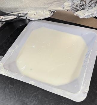
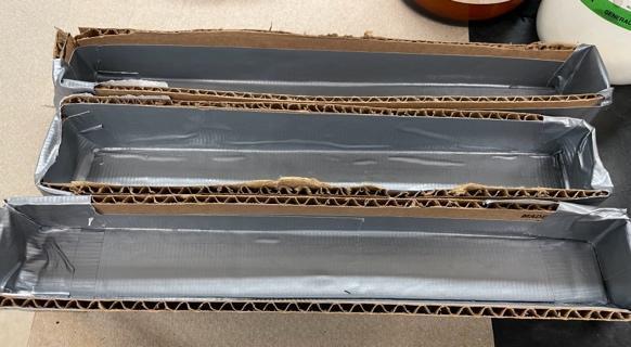
In order to prepare the final photographic plates, which should ideally be flat surfaces, two procedures for gelatin-set photographic media, inspired by Schaller and Mackenzie (8), were attempted. In the first, three molds (2.54cm by 25.4cm by 2.54cm) were constructed out of corrugated cardboard and waterproof tape, then labeled according to each of the final silver halides: bromide (AgBr), iodide (AgI), and chloride (AgCl). (Figure 3) In the second, each gel was set in a large weigh boat, then systematically covered and exposed to each frequency of light. (Figure 4)

In order to make each gel, 2.0g of an appropriate potassium or sodium halide was added to a 150 mL beaker, along with 2.5g of gelatin mixed in 25mL of distilled water, then heated to 50 C. In a separate 100 mL beaker, 25 mL of distilled water was mixed with a stoichiometrically

appropriate4 amount of silver nitrate (AgNO3), then heated to 40 C. (See Tables 1 and 2) The two ° beakers were mixed thoroughly in a dark environment under a safelight, allowed to cool for 10 minutes, then poured into their respective mold. The gels were cooled to approximately 5 C and ° allowed to set overnight.

Exposure for the preliminary salt precipitation and the cardboard set gels was procedurally identical. In a dark environment, an LED array consisting of eleven equally spaced colored lights was mounted an inch above the plate and exposed for approximately fifteen seconds.

Table 1. Proportions of halides, silver nitrate, water, and gelatin used in initial trials (no data collected). These amounts, though incorrectly calculated (see discussion), are reported for completeness.

4 In the first two (ultimately unsuccessful) trials, the amounts of silver nitrate in each experiment were 1-1.5g higher than stoichiometrically required (i e given by amount times ratio of molar masses times mole ratio) with the assumption that more impurities in the gel would serve as a doping agent, allowing more silver ions to collect. While a seemingly common amateur photographic practice, the overall efficacy of this remains to be tested (see Results/Discussion).

Nevins-Klein, Scientific Transactions of the Grayson Society, May 2025

Table 2. Proportions of halides, silver nitrate, water, and gelatin used in the final, data-gathering stage. These values were chosen to be consistent with Schaller, which includes 6.331g of the final silver halide salt per 150 mLs of water, though both the water and gel amounts were reduced from Schaller ’s original experiment.

RESULTS

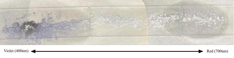
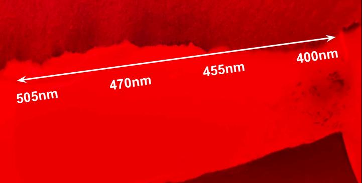
Given time constraints, only three iterations of the experiment were attempted. The preliminary AgCl salt precipitation was successful, despite less-than-ideal yield (approximately 70%) caused by product loss on the rimmed lip of the decanting vial. The resulting quantity of salt was enough to cover the 25cm filter paper, though the likely still high-water content in the salt meant that it was difficult to spread evenly Photoactivity measurements matched expected results, with significant activity in the violet region (350-435nm) and little other activity (Figure 7).

The first two gel experiments (Table 1, Trials 1 & 2) were ultimately a failure. The first iteration of the molds, which made

Nevins-Klein,

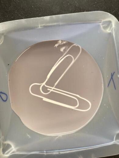
use of absorbent cardboard and permeable table disintegrated in the early stages of the gelatin setting and rendered all the gels, now set into the tray, unusable for experimental purposes. The second iteration, while somewhat sturdier, faced a similar issue and had to be discarded. Hasty calculation meant that these gels also used 1-2g less silver nitrate then required, and in particular the resulting potassium gel was barely photosensitive. Salvaged trays of silver emulsions (mainly silver chloride) were prepared and tested for basic photosensitivity using contact printing: a small object was placed on the surface of the gel and exposed with a violet flashlight.

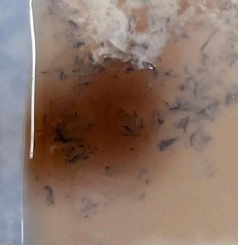
The second trial had mixed results. One gel (silver iodide) failed to set, and another (silver bromide) set completely dark and was impossible to distinguish when exposed to light, potentially indicating overly high sensitivity or a light leak. The third gel, silver chloride, yielded excellent, expected results with high reactivity to violet light, with a pronounced discoloration on the exposure surface under the violet ( ) LED (Figure 10). Also notable are the λ = 400�� presence of small, dark particulates, perhaps indicating large deposits of silver due to long exposure times.

DISCUSSION

The evidence reaffirms known experimental data about the preferred wavelengths of silver chloride and is inconclusive about the other silver halides, providing an avenue for further experiments or the creation of high-fidelity black and white photographic film.

In the first two (ultimately failed) gel-based trials, calculation errors would have meant that any data collected from the trials, had they been successful, would be significantly harder to use. To calculate the necessary mass in grams of one reactant, giving a fixed amount of another, limiting reactant, one uses basic principles of stoichiometry, converting the mass to a quantity in mols, multiplying by the mol ratio of the two reactants, and converting back to grams. I mistakenly switched the role of the two reactants and consequently multiplied by the reciprocal of the mass ratios, dramatically underestimating the amount of silver nitrate necessary, a mistake only partially offset by my decision to add more silver nitrate as a dopant. Thankfully, I caught this error before the third and final trial, and I don’t believe that this mistake has substantially affected the results of this paper

There are a few explanations for the partial failure of the third trial. The heating and cooling process of one of the gels (likely silver iodide) was left momentarily unsupervised. There is a possibility that the gel superheated, disrupting the structure of the gelatin and interrupting the gelling process. The amount of gelatin used was also approximately half that of Schaller, making setting tolerances more sensitive. The gels exhibited some unevenness at time of setting, indicating more mixing of the solutions is necessary

Future experiments could focus on more accurately measuring the photoactive ranges of silver salts, perhaps using a variable filter and digital analysis to determine the precise point of change. An experiment could also focus on the way that being set in a gel affects the optical properties of silver salt, and if factors such as gelatin concentration change required frequency and intensity of light.

Nevins-Klein, Scientific Transactions of the Grayson Society, May 2025

REFERENCES

[1] Witten, Nichole Marie. "Thesis: The Chemistry of Photography." 5 May 2016. University of South Carolina University Libraries, Scholar Commons 7 May 2025

[2] Boyd, Jane E "Silver and Sunlight " Distillations Magazine (n d )

[3] Johnson, Tim. Chemistry and the Black and White Photographic Process: The Making of a Negative . 2004. 6 May 2025

[4] Shikir et al "Impact of Mo doping on photo-sensing properties of ZnO thin films for advanced photodetection applications." Journal of Alloys and Compounds 985 (2024): 174009.

[5] Victoria, R H "Calculated electronic structure of silver halide crystals " Phys Rev B 56 (1997): 4417-4421

[6] Flowers, Paul Chemistry 2e Houston, Texas: OpenStax, 2019

[7] Rogge, Corina and Aniko Bazur. "19th Century Photography in a Modern Chemistry Lab." AIC Annual Meeting. Albuquerque, New Mexico, 2012

[8] Schaller, Robert and Alex Mackenzie "Basic recipe: unwashed emulsion " n d Film Labs

[9] Eder, Josef Maria. Quellenschriften zu den frühesten Anfängen der Photographie bis zum XVIII Jahrhundert. 1913.

ACKNOWLEDGMENTS

The author would like to thank American Scientific, Arbor Scientific, and Flinn Scientific for providing materials used in this experiment, Mr. Sizer, Head of Biological and Chemical Science at The Grayson School, for his continued guidance and support through all stages of the research process, and Nerya Friederich, Beatrix Lay, Beesan Muaddi, and the rest of the Scientific Inquiry class for their support in preparing samples. The scientific results and conclusions and any views or opinions expressed herein are those of the authors and do not necessarily reflect the views and policies of The Grayson School.

Funding: This experiment was supported by the Department of Science at The Grayson School. Competing interests: The author declares no competing interests.

License information: Copyright © 2025 the author Nevins-Klein,

Feasibility of piezoelectric energy harvesters at The Grayson School

Nerya Freidenreich✝

ABSTRACT

Piezoelectric energy harvesters (PEH) have received significant attention in the world of renewable energy innovations. In particular, studies into the feasibility and optimization of PEH for pedestrians, within buildings and other infrastructure, are an intriguing route for clean energy harvesting. This study aims to assess the efficiency and practicality of implementing PEHs at The Grayson School specifically.

INTRODUCTION

Piezoelectricity as a form of renewable energy generation has received dramatically increasing attention in the modern world of innovation. From 2000-2019, 1,172 papers were written about prospects in piezoelectric energy harvesting, and an additional 3,263 from 2019 to 2024 (1). A clean source of energy, with relatively easy implementation, piezoelectric generators seem to be a viable possibility for the future of energy technology.

Yet piezoelectricity, as a phenomenon, is far from being a new concept. First discovered by Jaques and Pierre Curie in 1880, piezoelectricity is an electric charge generated in response to mechanical stresses in certain solid materials (2). The piezoelectric effect is a reversible process, meaning that mechanical strain (vibrations, pressure, temperature, etc.) can produce electrical energy, and vice versa, electrical energy creating mechanical strain. It is also a dynamic process, such that the change in physical structure is what causes electrical output, not the state of the configuration itself (Fig. 1). In piezoelectric materials, application of external mechanical stress reconfigures dipole moments, thereby changing the polarization within the crystalline structure of the piezoelectric material. That change in polarization strength, dependent on the orientation of change in crystal symmetry and applied strength, appears as a

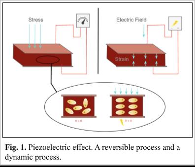
variation of surface charge density on the crystal faces, resulting in electric field and current generated. Voltage produced is directly proportional to the applied force of pressure or strain.

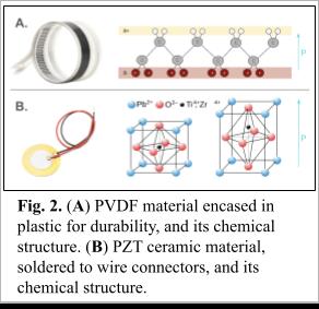
Sensitivity can vary depending on the piezoelectric material and how it is cut; ceramic materials, for example, have piezoelectric sensitivity roughly 2 orders of magnitude higher than quartz crystals (although crystals have longer durations of stability), and can be cut shear, transversely, or longitudinally (3). The most common piezoelectric ceramic is made of brittle lead zirconate titanate (PZT) crystals, which generate measurable piezoelectricity when structurally deformed by 0.1% of its original dimension (4) Recently, using polyvinylidene fluoride (PVDF) encased with a plastic film has garnered some attention as a piezoelectric, for its flexibility, high electrical output, and durability in comparison to PZT (Fig. 2). One study claims PVDF to have “10 times higher [high voltage output] than piezo ceramics for the same force input” (5) Although PVDF sensors are more temperature sensitive than PZT ones, they do offer a wider frequency compatibility range, high elastic compliance, and mechanical strength / impact resistance.

With advancements in micro- and nanoscale crystallization optimization and manufacturing processes, energy harvesting through piezoelectric generators has received much attention, due to its enhanced electromechanical coupling factor (in comparison to other electrostatic, electromagnetic, and triboelectric transduction options), flexibility, and miniaturization (6). Still, piezoelectric energy harvesting has some major limitations. The main concern is the ability to generate enough energy to make installation worthwhile. Technology is difficult to scale up and integrate into existing infrastructure, especially considering the geometric and circuit-related complexity of efficient piezoelectric energy conversion systems. Piezoelectric systems generate limited power output, to the order of microwatts for ambient vibrations, which may not be sufficient for powering high energy consuming devices. Other constraints include frequency and bandwidth limitations among individual piezoelectric materials, hysteresis and energy loss from lack of overall efficiency of the system, and environmental constraints and durability, considering extreme temperatures, humidity, and degradation due to long term mechanical stress (7).

Keeping in mind such limitations, piezoelectric energy harvesting systems have been successfully applied to commonplace activities, ranging from vehicle motion1, weather and

1 Piezoelectric roads work conceptually by converting vibrations from traffic into energy using PEHs embedded beneath asphalt, which can then be linked either to a collection point next to the road, or directly to the grid as Freidenreich, Scientific

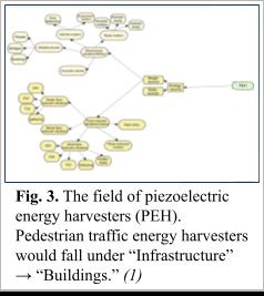
fluid-induced motion (8)(9), and animal/human bodily motion (10), to name a few (Fig. 3).

Piezoelectric infrastructure in walkways and buildings, specifically, has gained some public attention around the world. The idea is to replace some floor tiles with piezoelectric tiles, which will generate electricity in high pedestrian traffic areas as people walk over the floor. It is estimated that 1000 steps of an average human walking could produce nearly 80 W of power (4).

Maximizing energy output for piezoelectric walkway infrastructure involves multiple considerations. A) the resonant frequency of the piezoelectric energy harvester (PEH) should match the dominant frequency of motion. B) Heavier people create more energy, as do taller people. C) The average power gained from going downstairs is significantly higher than for going upstairs. D) Orientation of the PEH significantly affects the total amount of harvestable energy. E) Available potential energy for harvesting is directly proportional to tile deflection; the more flexible the floor tiling, the better2. However, this must be balanced with F), the mechanical stiffness of the walking surface, which plays an important role in controlling the human gait cycle. For largest success, a floor tile energy harvester should have similar deflection and stiffness to the rest of the floor.

Foot traffic pattern analysis goes hand in hand with piezoelectric walkways, both because PEHs allow for real-time monitoring of foot traffic, but also because finding the optimal placement of a piezoelectric walkway, using the considerations above, requires locating (using traffic pattern analysis) the highest traffic areas, the direction of traffic flow, demographic of walkers, and density flow per unit time.

There are many designs previously both created and implemented for PEHs for pedestrian traffic flow. Most commonly used is the PZT ceramic, but it can be limited due to its

2 In Virginia, there is a construction code detailing the maximum allowable deflection of a floor, making many piezoelectric tile designs, such as those created by Pavegen, illegal to install in buildings

another electrical input (11). The network of generators beneath the road has been arranged both in thin strips perpendicular to the lanes or as tiles running parallel to the lanes, and implemented successfully into both highway systems and airport runways. An Israeli company, Innowattech, for example, installed piezoelectric materials under a busy highway in 2009, and claimed to generate enough electricity to power 300-600 homes within 24 hours In 2011, piezoelectric crystals were installed under a stretch of road from Trieste to Venice. Saafi et al. (Lancaster University) tested one mile stretches in the UK and Italy, and measured 2 MW per km under normal traffic volumes (2,000-3,000 cars per hour), using that energy to power street lamps, traffic lights, and electric car charging stations (12) They found that the biggest challenges were cost, durability, and compatibility with asphalt and vehicle gas consumption. From 2017-2023, UC Merced installed and tested 2 cm wide multi-layer PZT piezoelectric generators on a 200 ft span of asphalt, and concluded the potential for 72,800 kilowatt hours of energy per year on a one-mile long roadway, and around 907,000 kWh with heavy trucks They also predicted a 4000 metric ton reduction of carbon dioxide, and calculated that outfitting all 386,604 miles of lanes in California with piezoelectric energy harvesting devices would yield a CO2 reduction of 115 million metric tons annually (13) Freidenreich,

brittle nature (14). To make it more durable, PZT is either paired with carpet (3.8 watts per step), or wood (2.9 W/step) (15). Otherwise, PVDF is used in a film form, usually encased in thin plastic for increased longevity.

Converting the mechanical energy into electrical energy for use requires a storage capacitor. The discontinuous nature of footsteps makes the power generated ill-suited for powering ordinary electric devices, which require continuous power. There is also typically not enough instantaneous energy produced by each footstep at a given time. Intermittent storage capacitors are required to accumulate the energy until a signal transmission can be powered.

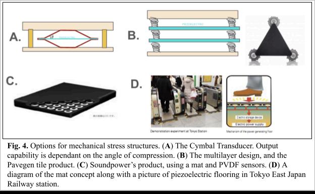
Options for mechanical stress structures are as follows (Fig. 4). As discussed above, highly flexible floors, often implemented on dance floors, generate electricity from the mechanical stress of bending and fluctuating pressure amplitudes, but they become less effective over time, requiring large deflection (up to 10mm) to be effective (10).

One design is the cymbal transducer, which has a strip of piezoelectric material strung between two trapezoidal hollow metal sheets, which when applied pressure, compress and apply stress on the piezoelectric interface. The amount of energy generated in this case is largely dependent on the angle of compression, with the largest amount of power possible equaling the furthest loaded state possible, and the limiting factor being the stress maximum in the piezoelectric layer3 (16). Usually this setup is estimated to output at the most 53 mW/step (17).

3 Virginia Tech did a study on the number of cymbal transducers optimal in a tile, finding that the number of transducers in a tile determines the stress each one experiences; the stress is distributed relatively evenly The more transducers used, the more potential energy can be harvested before the cymbals each become overloaded They found that the optimal number of transducers for an NFL football player sized person is 14, 8 for the average adult, and 6 for the average child

Freidenreich, Scientific Transactions of the Grayson Society, May 2025

Another option is a multiplayer stacked structure, where piezoelectric surfaces are compressed into four or more thin layers, with bars inside to apply pressure on the piezoelectric stacks inside the tile (18). The design’s efficiency is usually dependent on the orientation of the piezoelectric columns, with an expected maximum output of 129 mW assuming a 60 kg weight (19). Multiple commercial products using this technique can be found, including Pavegen, who advertises that each tile has wireless API device for transmitting real-time movement data analytics while funnelling power to specific areas, powers interactive messages, billboards, and to track footfall hotspots. A study by X. Li et al. at Macquarie University in Sydney Australia, integrated 1820 Pavegen tiles (3.1% of their total floor area) into a central hub building on their university campus, and calculated a total annual energy harvesting potential in an optimized model of 9.9 mWh/year, close to 0.5% of the annual energy needs of that building (8) (20). Other companies, such as Wayenergy Flooring, and Sustainable Energy Floor (SEF) have similar designs and energy output efficiencies (21)

Alternatively, rubber mats containing piezoelectric sensors require no deflection of the ground. Rather, the efficiency depends on the thickness of the mat, the force of the pedestrian, and the properties of the piezoelectric material (usually PVFD instead of PZT for durability and cost-cutting). Higher force and larger thickness generate a higher amount of surface changes. This design was implemented in 2008 at Shibuya station and Tokyo East Japan Railway stations, Japan, where footstep sensing floors harvested the crowd’s kinetic energy for powering the ticket gate operators and display systems (22) Using a 2.5 cm thick mat, and generating electricity in real time, along with a light display board that updates the amount of electricity created, they estimated that 2.4 million people pass through everyday, and that a person weighing 135 lbs generates 0.1 watts in the second they take to step on the time. Another company, Soundpower, uses a similar technology set up for applications in emergency stairwells, advertising a similar energy output of 0.1 watts (21)

In this study, the feasibility of piezoelectric walkway technology was investigated at The Grayson School. The inquiries for analysis were threefold: 1) What are the traffic patterns of an average school day? 2) How much electric energy can be produced from foot traffic on a given day? 3) How feasible and worthwhile is a piezoelectric set up at The Grayson School?

MATERIALS and METHODS

Material and Structure of PEH.

Originally, a design was created based on the cymbal transducer method. Creating mini transducers, bottle caps were used as plastic versions of the metal trapezoidal structure, with PZT piezoelectric disks suspended from the rim of the cap, creating a deflection when pressure was applied. Ten of these transducers were placed in series. Secondly, the mat method was implemented with a PVDF piezoelectric strip placed under a 1 cm thick carpet mat (Fig. 5). Testing both structure options with a voltmeter yielded a 3 ± 1 mV when force was applied.

Electrical connection of PEH.

The PEH was connected to a 10 bit analog input on an Arduino Uno microcontroller, with the piezoelectric wired in series with a 10Ω resistor to create a voltage divider (Fig. 6). The voltage divider was necessary in order for the analog pin of the microcontroller to detect changes in voltage. The Arduino generated 5 volts, and the voltage received by the analog pin fluctuated as the resistance in the PEH changed. The input values ranged between 0-1023, and a threshold of 1000 was established to reduce the hysteresis effect observed from the PEH. When pressure was applied on the PEH and the input exceeded 1000, an LED was turned on to give a visual indication that the PEH had detected a footstep. The LED would turn off whenever the input was less than 1000. While the light turning on was not directly powered by the piezoelectric system, it provided physical evidence of a significant enough change in resistance and voltage, corresponding to a wattage increase. The circuit was hooked up to an LCD screen, which displayed the real-time resistance levels along with the number of footsteps calculated. Implementing the PEH into The Grayson School.

Considering that more mechanical stress is placed when going down stairs, and keeping in mind the layout / traffic flow of The Grayson School, the PEH was placed in the stairway landing, directly by the front door. The piezoelectric PVDF strip was placed perpendicular to normal traffic flow, with the Arduino element and computer program tracker placed underneath the stairs (Fig. 7).

Reading the data.

Data was collected over the course of a week and a half. Some trials went overnight, some only during school hours. Data was collected at a baud rate of 9600 by the serial port of

RESULTS

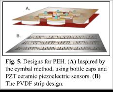
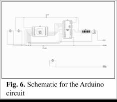
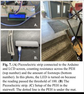
the Arduino IDE, and fed directly to a rust app created specifically to read any RS-232 data from Arduino and sensors connected to them (Fig. 8). The program both tracks and records sensor signals, and also graphs them in real time. The data is all the while saved natively from the port for each open graph while the code is running, and can be saved as either raw byte or as CSV. From the CSV file, more data analysis was performed using Microsoft Excel.

The original cymbal design was unsustainable, largely because of durability issues. The PZT was flimsy, especially in the soldering of the wire connection, and would have needed much more severe structural protection to be usable for the PEH. Meanwhile, the PVDF strip was encased in plastic, which made it strong but flexible. In addition, the PVDF had more sensitivity and frequency range than the PZT, making it the better candidate overall.

The PVDF strip measured a change in resistance of >800 Ω per footstep. Results were taken continuously over the course of multiple days, and each day measured in the range of 30,000 steps. As an individual’s weight landed on the strip, the sensor did respond accordingly with a spike in voltage through the system, a difference of 3.34 ± 1 V, and the voltage measured from a footstep ranging from 3.9 to 4.8 V (depending on whether the piezoelectric sensor strip was under the mat or not. It was more sensitive without the mat). It is evident, based on the graph, that the sensor was working well. One can see the increase in sensor activity during the hours of 8:00 am - 4:30 pm, exactly corresponding with the hours people are in the building (Fig. 9). However, during times when footsteps were measured, there was often acute hysteresis, to the point where the sensor would register a footfall up to a minute after the weight was removed, making analysis of traffic flow hard to measure.

DISCUSSION

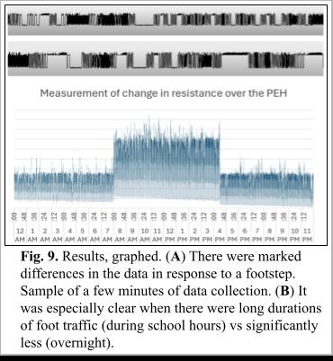
Results were mixed. On the one hand, the sensor was successful in measuring footsteps and calculating changes in resistance, and equally successful in measuring the lack of footsteps when there were long periods of no foot traffic. There was also enough traffic flow to register significant resistance data points throughout the school day using the PVDF based PEH. However, limitations with the Arduino technology and hysteresis made it hard to analyze and make definitive conclusions about both the traffic flow patterns and the amount of energy available for harvesting during school hours.

Contributing to the inability for traffic cycle analysis, only one sensor strip was used, due to the timeline of the project, but having multiple piezoelectric strips would have yielded better, more conclusive data, along with a much larger energy harvesting capability.

Another aspect to note is the uncertainty in how much of the population actually stepped on the sensor, as supposed to avoiding it altogether. This issue is twofold. First, although the sensor itself was hidden relatively inconspicuously underneath a mat, wiring gave it away as irregular flooring, and combined with certain teachers misguidedly advising others not to step on the mat or touch the sensors, for fear of tampering with the project, its estimated that less people stepped on the sensor than would normally step on that area of the floor otherwise. Secondly, it is crucial to note how the placement of the PEH on the stairway structure might have impacted its success. The PEH was placed, for this study, so that it bisects the landing, but considering the average adult gait cycle when going up and down stairs in a rush, it was noticed that the chosen area might be skipped over. Positioning the PEH at a different angle on the landing might yield different results (Fig. 10).

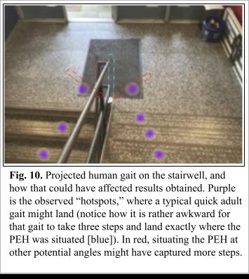
Overall, implementing a piezoelectric harvester system into The Grayson School is effective in getting students to talk about new sources of renewable energy, however results were inconclusive as to how feasible and efficient the structure would be within a school setting.

ACKNOWLEDGEMENTS

The author would especially like to thank Blaise Baptist for the use of his program for data collection, without which this study would not have been possible. Many thanks also to Marcus Baptist, Tani Nevins-Klein, Jordana Wilkes, and Dr. Colin Tinsman for their technical expertise on Arduino functioning. Deep gratitude to Mr. Michael Sizer for his continued support, guidance, and encouragement throughout the project.

The scientific results and conclusions and any views or opinions expressed herein are those of the author and do not necessarily reflect the views and policies of The Grayson School, Delaware County, or the US government and its agencies.

Funding: This experiment was supported by the Projects Department in collaboration with the Scientific Inquiry and Experimental Design program at The Grayson School.

Competing interests: The author declares no competing interests.

REFERENCES.

[1] Ghazanfarian, J , Mohammadi, M M , & Uchino, K (2021) Piezoelectric Energy Harvesting: A Systematic Review of Reviews. Actuators, 10(12), 312. https://doi.org/10.3390/act10120312

[2] What is Piezoelectricity? | OnScale (n d ) OnScale Solve Retrieved May 6, 2025, from https://onscale com/piezoelectricity/what-is-piezoelectricity/

[3] Damjanovic, D.. (2005). Piezoelectricity, Encyclopedia of Condensed Matter Physics, ISBN 9780123694010, Piezoelectric Materials (pp. 300-309), https://doi.org/10.1016/B0-12-369401-9/00433-2.

[4] Chakraborti CS PhD, S (2016) Harnessing Piezoelectricity for daily use::From footwear to lamps Rochester University

[5] Measurement Specialties, Inc. Sensor Products Division. (1999). Piezo Film Sensors Technical Manual. https://cdn sparkfun com/assets/d/a/a/b/b/Piezo Film Sensors Technical Manual pdf

[6] Sezer, N, Koç, M (2021) A comprehensive review on the state-of-the-art of piezoelectric energy harvesting, ISSN 2211-2855, Nano Energy Vol. 80, https://doi.org/10.1016/j.nanoen.2020.105567.

[7] Challenges And Limitations Of Piezoelectric Energy Conversion (n d ) FasterCapital https://fastercapital com/topics/challenges-and-limitations-of-piezoelectric-energy-conversion html

[8] Ilyas, M.A, Swingler, J. (2015). Piezoelectric energy harvesting from raindrop impacts, ISSN 0360-5442, Energy, Vol 90, Part 1, (pp. 796-806), https://doi.org/10.1016/j.energy.2015.07.114.

[9] Honde Technology, Co , Ltd (2025) Piezoelectric Rain And Snow Sensor: A New Breakthrough In Intelligent Monitoring https://www.hondetechco.com/news/piezoelectric-rain-and-snow-sensor-a-new-breakthrough-in-intelligentmonitoring/

[10] Qian, F , et al (2022) Bio-inspired bistable piezoelectric energy harvester for powering animal telemetry tags: Conceptual design and preliminary experimental validation. ISSN 0960-1481, Renewable Energy, Vol. 187, (pp 34-43), https://doi org/10 1016/j renene 2022 01 018

[11] Fadat, Y (2024) Energy Harvesting with Piezoelectric Roads: The Future of Sustainable Power Evolution of the Progress. https://evolutionoftheprogress.com/piezoelectric-roads/#google vignette

[12] Hurley, B (2017) A Piezoelectric Highway? Engineers Take Another Test Drive Tech Briefs https://www techbriefs com/component/content/article/27598-a-piezoelectric-highway-engineers-take-anot her-test-drive

[13] Sun, J.Q., Tian-Bing, X., Atousa, Y.. 2020. Ultra-High Power Density Roadway Piezoelectric Energy Harvesting System California Energy Commission Publication Number: CEC-500-2023-036

[14] Shreeshayana, R , Raghavendra, L , & Manjunath, V G (2017) Piezoelectric Energy Harvesting using PZT in Floor Tile Design International Journal of Advanced Research in Electrical, Electronics and Instrumentation Engineering, Vol. 6(Issue 12,), 1-8. DOI:10.15662/IJAREEIE.2017.0612018

[15] Shariffundin, P (2021) Piezoelectric energy floor tiles performance and effectiveness as building energy conservation measures for different types of buildings in Malaysia http://eprints.utar.edu.my/5210/1/Project 2000717.pdf

[16] Sharpes, N., Vučković, D., & Priya, S. (2015). Floor Tile Energy Harvester for Self-Powered Wireless Occupancy Sensing De Gruyter, Energy Harvesting and Systems, 1-19 DOI 10 1515/ehs-2014-0009

[17] Nia, E M et al (2017) A review of walking energy harvesting using piezoelectric materials Materials Science and Engineering 291 (2017) 012026 doi:10.1088/1757-899X/291/1/012026

[18] Song, G J et al (2019) Development of a pavement block piezoelectric energy harvester for self-powered walkway applications, ISSN 0306-2619, Applied Energy, Vol 256, https://doi.org/10.1016/j.apenergy.2019.113916.

[19] Elnaklah, R , & Rumman, S A (2024) Investigating the Energy Generation Potential of Piezoelectric Flooring in Educational Buildings IV International Conference on Electrical, Computer and Energy Technologies (ICECET 2024), Sydney-Australia.

[20] Li, X., Strezov, V. (2014). Modelling piezoelectric energy harvesting potential in an educational building, [21] ISSN 0196-8904, Energy Conversion and Management, Vol 85, (pp 435-442) https://doi org/10 1016/j enconman 2014 05 096

[22] Elhalwagy, A., Ghoneem, M., Elhadidi, M. (2017). Feasibility Study for Using Piezoelectric Energy Harvesting Floor in Buildings’ Interior Spaces, ISSN 1876-6102, Energy Procedia, Vol 115, (pp 114-126), https://doi org/10 1016/j egypro 2017 05 012

[23] Fermoso, J. (2008, December 17). Power Generating Floor in Train Stations Light Up Holiday Displays. WIRED https://www wired com/2008/12/power-generatin/

[24] Piezo Generators: How They Work | APC International (n d ) American Piezo https://www.americanpiezo.com/knowledge-center/piezo-theory/generators/

[25] Piezoelectric Generator : 7 Steps (with Pictures) (n d ) Instructables https://www instructables com/Piezoelectric-Generator-1/

Investigation into the thermal properties of five metals and their salts

Rena L. Civan1

ABSTRACT

This study investigates the thermal properties of five metals (cobalt, copper, iron, tin, and zinc) and their salts when combined with sulfate and chloride ions, and in particular, the properties of specific heat and enthalpy of solvation. Data is collected through constant pressure, or isobaric, calorimetry, and analyzed using equations and properties discovered by scientists including Joseph Black, Germain Hess, Pierre Louis Dulong, Alexis Thérèse Petit, and Max Born.

INTRODUCTION

In the mid-eighteenth century, Joseph Black began a study into the nature of heat. Along with establishing the idea of latent heat, which describes the phenomenon of added heat not changing the temperature of matter on the cusp of a phase change, he also formalized what he referred to as capacity for heat, which is now known as specific heat. In a lecture he gave at the University of Edinburgh, Black described that despite what many of his contemporaries believed, there was a distinction between the temperature of an object and the amount of heat contained in it. He justified his stance with Daniel Gabriel Fahrenheit’s experiments comparing the way mercury and water interact with heat. When combining equal parts of the two fluids, each at a measured temperature, water had a greater effect on the resulting mixture’s final temperature, despite mercury being over thirteen times denser. The difference in effect turned out to be in a fixed ratio, with two parts water having the same power as three parts mercury. Another experiment further proved the difference between the fluids when mercury placed near a fire rose in temperature much more quickly than the same volume of water at the same distance. The same pattern in rate of temperature change was observed when cooling the fluids as well. Black reasoned from these experiments that water must have a higher capacity for holding heat. He conjectured that this capacity was a property unique to each type of matter (1).

The modern formalized concept defines specific heat as the increase in heat required to raise the temperature of a mass unit of a substance by a given amount, and often measured in joules per gram per degree Celsius. It is found experimentally through use of the equation , where c is the specific heat, q is the heat added, m is the mass, and Δt is the � = �/(� · ∆�) change in temperature (2). Black was able to make these deductions which still hold true to our modern understandings, despite working in a previous framework of the caloric theory.

The theory argued that heat was made up of a liquid known as caloric that flowed between matter. Caloric was thought to be self-repulsive which would explain the tendency for temperatures of objects in a closed system to equalize, and its volume would always be

1 Corresponding author, rcivan@thegraysonschool org Civan,

conserved. The theory was quite prevalent, and believed by many prevalent scientists of the era including Benjamin Franklin and Antoine Lavoisier (3).

One of the first scientists to take on caloric theory was nineteenth century physicist James Prescott Joule. He described an experiment done by Sir Humphry Davy where he rubbed two pieces of ice together in a cold vacuum. While there was no initial “caloric” in the system, the friction between the pieces of ice created enough heat to melt some of the ice. Joule sought to formalize the relationship between heat and mechanical work. Using a brass paddle wheel propelled by dropping weights to agitate a sealed vessel of water, he deduced that it took 773.64 foot-pounds of work (equivalently, 1048.915 Joules) to raise the temperature of one pound of water one degree Fahrenheit (4).The amount of energy required to raise the temperature of one pound of water by one degree Farenheit was such a relevant quantity that it became the basis for the British thermal unit, a unit now used mainly for heating and cooling systems as well as fuel (5). Analogously, a calorie is the unit of energy required to raise the temperature of one liter of water by one degree Celsius or Kelvin, and it is often used to describe the energy contained in food (6).

This still left questions of what, if any, patterns or equations could predict the specific heat of a given substance. Pierre Louis Dulong and Alexis Thérèse Petit found that the heat capacity per mole of many metals is approximately equal to a common constant from empirical data. This constant was later found to be around three times the universal gas constant R (approximately 8.31 J/mol/K), making the law’s approximate specific heat of metals to be 24.94 J/mol/ºC (7). Since specific heat is easier to find experimentally than atomic weight, the equation proved to be a useful tool for molar mass calculations. In 1865, Kopp’s law used more data to extend the pattern to include more chemical compounds. Gilbert Newton Lewis also confirmed this law experimentally for a number of solids at 20 ºC in a 1907 paper (8). Though the pattern produces good approximations for common substances at medium temperatures, it quickly becomes a worse approximation at extreme temperatures and for substances of very low or high masses (7).

Building on Ludwig Boltzmann’s 1877 explanation involving harmonic oscillators, Albert Einstein postured that specific heat can be described by quantum harmonic oscillators. His theory took atomic vibrations into account and held up better for wider ranges of temperature, especially on the higher end (9). In 1912, Peter Debye put forth his own, adjusted, model, which also looked at the phonon, defined as the collective excitation or vibration of particles in condensed matter, contribution to specific heat (10).

When looking at the behavior of compounds, it can also be helpful to consider another property, known as enthalpy. Enthalpy is defined as a system’s internal energy added with the product of its pressure and volume. The change in enthalpy of a system is used to describe bond, lattice, formation, and solvation energies. Enthalpy of formation refers to the amount of energy needed to produce a mole of a product from its elements. In 1840 Germain Hess determined that it is a state function, meaning that given a set of specific initial reactants and final products, the

change in enthalpy does not depend on the intermediate steps of the reaction. This statement became known as Hess’s Law (11).

The measurement of change in enthalpy is a technique known as calorimetry. Since it was first used in 1789 by Lavoisier and LaPlace, there have been many forms of calorimetry including constant pressure (isobaric) calorimetry, constant volume/bomb (isochoric) calorimetry, and differential scanning calorimetry (12). All calorimetry performed in this paper would be considered constant pressure calorimetry at atmospheric pressure. The general approach behind it is to have some process in question occur in an insulated vessel of water, measure the change in temperature, and use the specific heat of water to determine the heat released or taken in by the process.

This paper seeks to explore the thermal properties of five metals, namely copper, iron, zinc, tin, and cobalt (Fig. 1). These were chosen as they are all relatively easy to obtain and safe to work with and all can form cations with a positive charge of two. The properties explored are the specific heats as well as the enthalpy of solvation of their salts formed with one sulfate anion (SO42-) and with two chlorine anions (Cl-). Since energy is conserved, the enthalpy of solvation, or the heat exothermically released into the water or endothermically taken in, should be the negative of enthalpy of formation.

The energy contained in the ionic bonds a crystal structure is known as the crystal's lattice energy Specifically, lattice energy refers to the energy it takes to convert between one mole solid ionic compound and its ions in gaseous form. The process of switching from gaseous ions ionic crystals is always exothermic, and the reverse is always endothermic, as the crystal state is more stable. The value is affected by the charge of the ions, positive and negative two for the salts examined here, and the distance between ions which itself is dependent on a number of factors including atomic radii and crystal structure. While in most cases, lattice energy cannot be measured directly, there are a number of equations and processes to approximate it including the 1918 Born-Landé equation, the 1919 Born-Haber Cycle, the further refined 1932 Born-Mayer equation, and the 1956 Kapustinskii equation. The Born-Haber cycle is typically the best way to estimate it using experimental data. Based on the conclusions of Hess’s Law, the cycle states that heat of formation is equal to the sum of the energy released from electron affinity forming the anion and lattice energy minus the sum of the sublimation energy of the metal, the dissociation or atomization energy of the substituents, and the ionization energy to form the cation. It can be expressed as the equation ΔHformation° = ΔHsublimation° + ½ D + IE - ΔHlattice - EA (13). Depending on the crystal, enthalpy of formation can either be positive or negative.

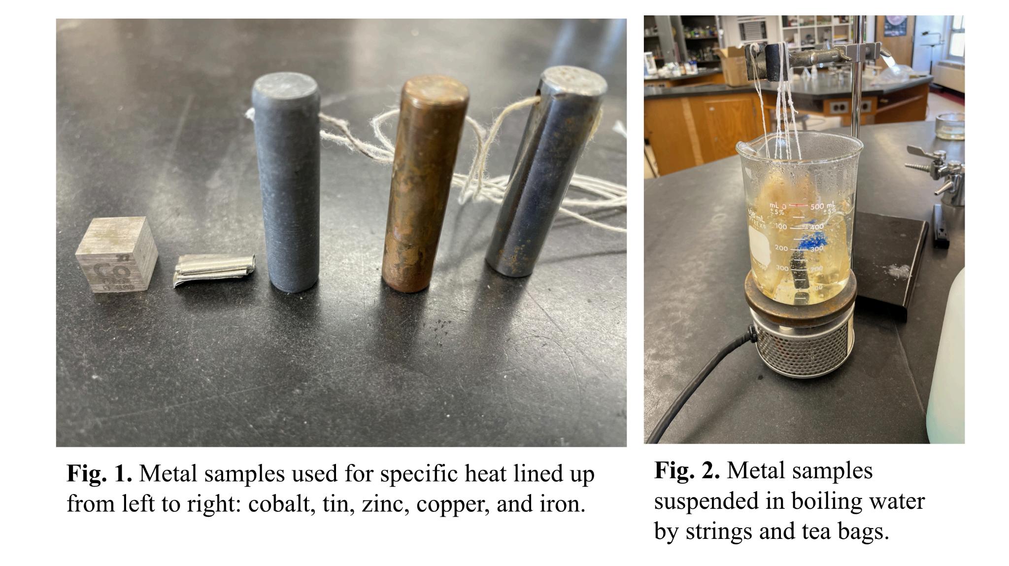
The salts obtained specifically were copper (II) chloride dihydrate, copper (II) sulfate pentahydrate, iron (II) chloride tetrahydrate, iron (II) sulfate heptahydrate, anhydrous zinc (II) chloride, zinc (II) sulfate heptahydrate, cobalt (II) chloride hexahydrate, cobalt (II) sulfate heptahydrate, and anhydrous tin (II) chloride). While initially tin (II) sulfate was intended to be used so that all five metals could be tested with sulfate anions, the salt was determined to be too deliquescent for this procedure, meaning it absorbs moisture from the air and dissolves in it (14). Hydrate crystals form when water, a dipolar molecule, is attracted to the charged ions of the salts; they are named with a prefix indicating the degree of hydration, meaning the ratio of moles of water to moles of salt. The degree of hydration of a crystal can affect properties from color to solubility to stability (15). The salts used in this study were chosen because they were all among the more stable varieties and water soluble.

MATERIALS and METHODS

First, specific heat analysis was performed on samples of each metal. The copper, iron, and zinc samples were 27.217 g, 24.015, and sourced was only 9.227 weighed, then placed to heat them to 100ºC. move them between the and tin were contained then submerged in 100 (≈ 22ºC) in a calorimeter digital thermometer that the system reached recorded. Since the tin was used for greater precision. was repeated three times. Using the equation with the water mass, change � = �/(� · ∆�) in water temperature, and a value of 4.184 J/g°C for the specific heat of water, the heat was calculated. This heat absorbed by the water was assumed to be equal to the heat released the metal. The metal’s specific heat was calculated by dividing the released heat by the metal’s mass and the change in temperature. While eight of the nine salts tested were sourced in solid form, the cobalt (II) sulfate was sourced as an aqueous solution. 65 mL of 0.1 cobalt sulfate solution was transferred to

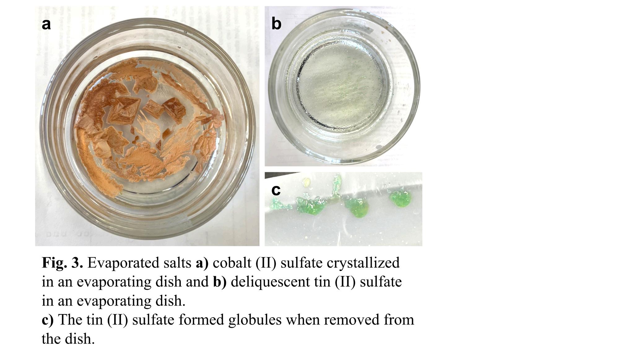
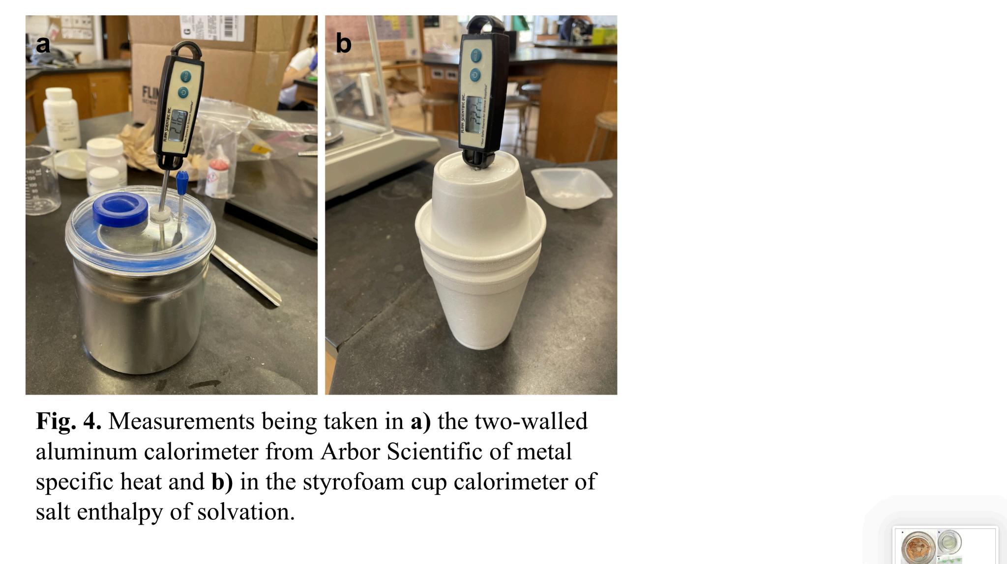
evaporating dish for several days to crystallize. A similar attempt was also made with aqueous tin (II) sulfate, however because of its deliquescence the salt was not used further (Fig. 3). T the enthalpy of solvation when water, approximately two added to one hundred calorimeter and the change salts dissolved was specific heat measurements, calorimeter with two with styrofoam, the done in a calorimeter cups as aluminum has of the ones used, and interfering with the equipment (Fig. 4). gently and consistently swirled until the salt was fully dissolved. The amount of heat this motion could have added was considered less impactful to the results as the potential for heat to dissipate from the calorimeter if the salts took several hours to dissolve without mechanical help. The salts were each given three trials with two exceptions: the cobalt (II) sulfate heptahydrate had one trial as only 1.3 grams was collected from the evaporation and the anhydrous tin (II) chloride was given an extra trial in a higher salt to water ratio as the thermometer was not sensitive enough to pick up any change in temperature in the standard ratio.

RESULTS

When using the specific heat formula for each trial, then averaging the results of the three trials the cobalt yielded a specific heat value of 0.305 J/g/ºC, the copper 0.341 J/g/ºC, the iron 0.393 J/g/ºC, the tin 0.342 J/g/ºC, and the zinc 0.349 J/g/ºC. When compared to literature values, the three metals with larger samples, copper, iron, and zinc, gave percent errors in the 10-12% range. The cobalt gave an error of around 27% and the tin 61%. The Dulong-Petit Law approximations were also considered, and found to all have percent errors in the 0.5-2% range

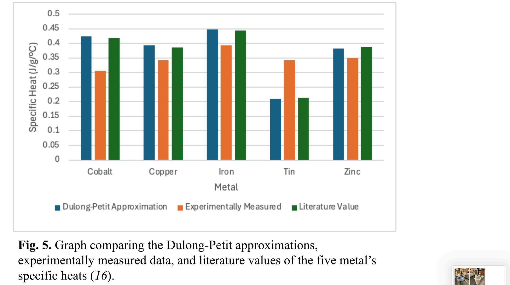
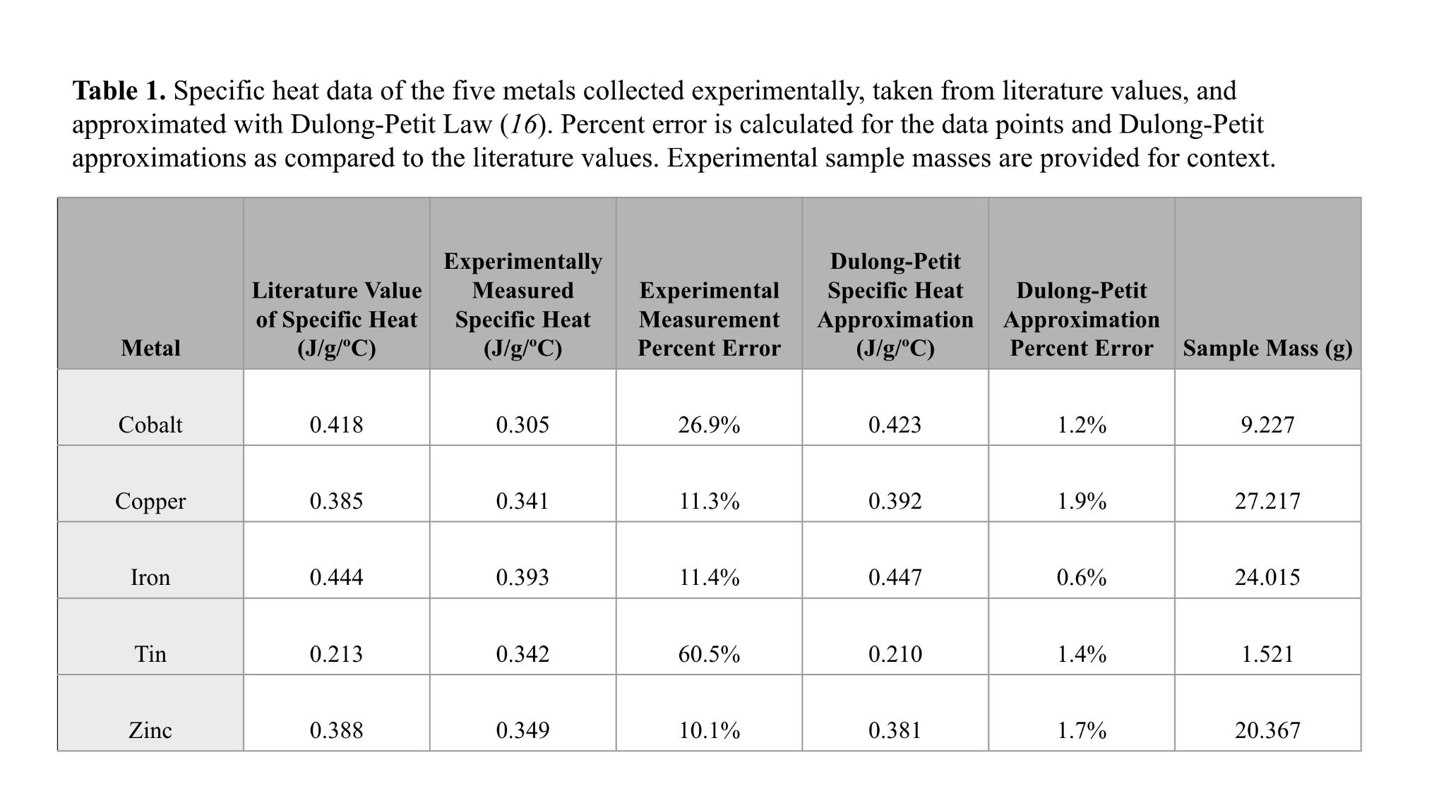
as compared (Fig. ) ( ). unfortunate, expected as, due to its small mass, the digital thermometer only measured a 0.1 ºC increase in every trial, the smallest increment the instrument gives. Notably, in the one trial where the water mass was reduced to around 50 g, the specific heat calculated was 0.188 J/g/ºC, with only a 12% error as compared to the literature value.

In terms of enthalpy of solvation, copper (II) sulfate pentahydrate, zinc (II) sulfate heptahydrate, cobalt (II) chloride hexahydrate, and cobalt (II) sulfate heptahydrate were found to be endothermic while copper (II) chloride dihydrate, iron (II) chloride tetrahydrate, iron (II) sulfate heptahydrate, zinc (II) chloride (anhydrous), and tin (II) chloride (anhydrous) were exothermic (Table 2). The anhydrous zinc (II) chloride appeared the exothermic, around 59,000 measured, cobalt (II) chloride hexahydrate most endothermic around -9,600 measured. There not appear to correlation enthalpy of solvation between salts same cation or anion. Civan,

DISCUSSION

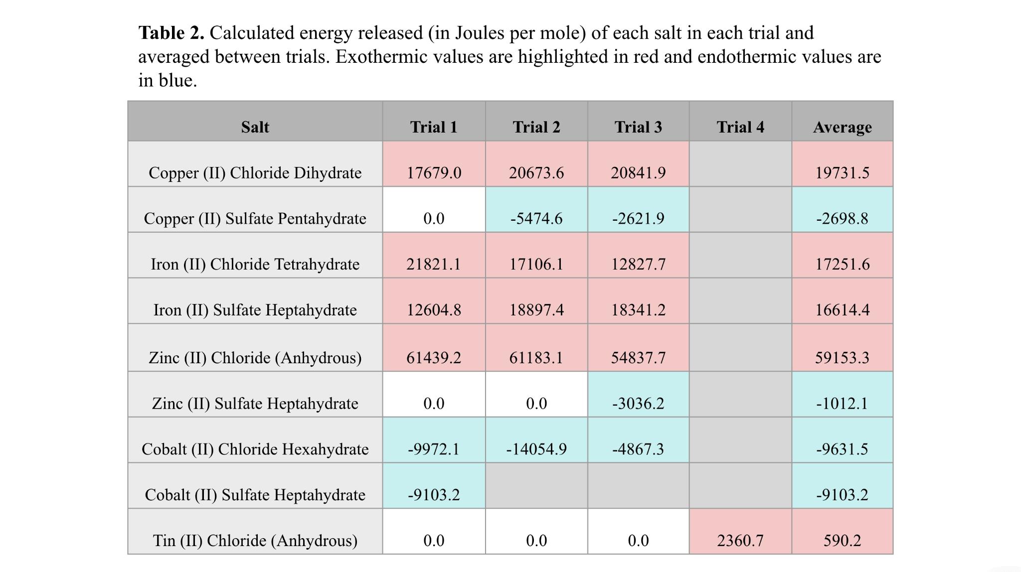
With the calculated enthalpies of solvation, the Born-Haber cycle could be used to find the lattice energies of the salts. While modifications would be needed from the cycle described here for the hydrous crystals, the lattice energies of the anhydrous salts are fairly straightforward to use with the equation. Using the calculated average 59.15 kJ/mol enthalpy of formation of zinc (II) chloride, the resulting lattice energy is 2253 kJ/mol; for tin (II) chloride when using the calculated average enthalpy of formation of 0.5902 kJ/mol, the resulting lattice energy is 1846 kJ/mol (Fig. 6).

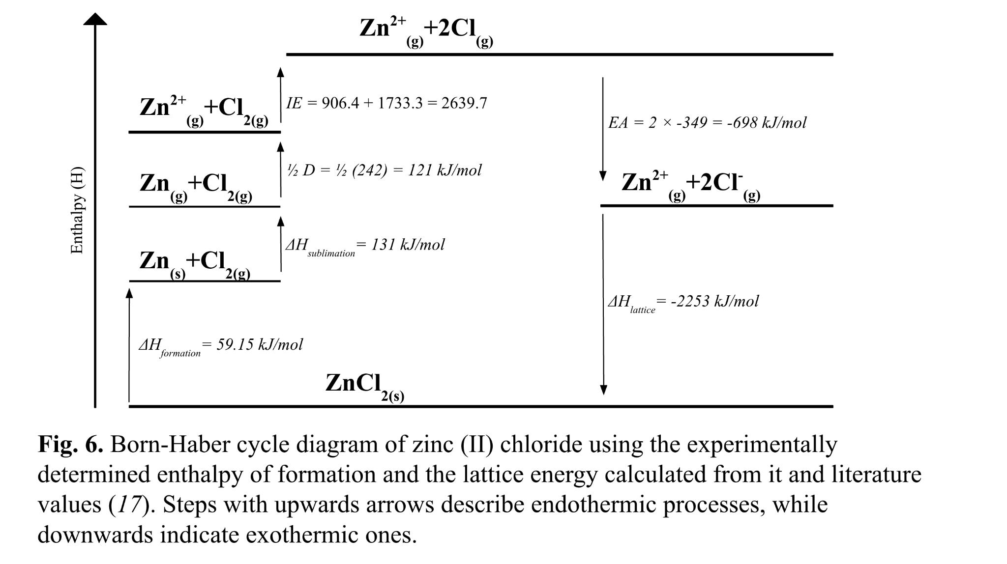
The measured values both for specific heat and enthalpy of solvation differed significantly from literature values. While there are many potential sources of error including thermometer precision, insulation of calorimeters, and purity of samples, the gest factor was likely the amount of water used relative to sample mass. The amount of temperature change measurable in the water from a given process is inversely related to the volume of water used. One hundred grams of water was a useful amount of water for these experiments because of the calorimeter setups and thermometer sizes, however when there was limited choice in metal samples for specific heat measurements and limited salts for enthalpy of solvation, the water volume proved to be an obstacle. This was especially difficult to overcome because the thermometer available could only measure in increments of tenths of a degree celsius. If the same procedure were to be repeated in larger calorimeters with higher sample to water ratios or more precise instruments, the accuracy would likely improve. Given more time and resources it would be interesting to repeat this experiment with more directly analogous salts of various metals. For instance, anhydrous chloride salts of all the metals or all heptahydrate sulfates. With isomorphic crystals, which vary only in ion, the correlation with other properties could be better investigated. Potentially correlated properties to further explore include cation molar mass, atomic radius, and specific heat.

ACKNOWLEDGMENTS

I would like to thank M. Sizer for his expertise, support, and guidance, as well as N. Freidenreich for her assistance.

The scientific results and conclusions and any views or opinions expressed herein are those of the author and do not necessarily reflect the views and policies of The Grayson School, Delaware County, or the US government and its agencies.

Funding: This experiment was supported by the Department of Science, The Grayson School. Competing interests: The author declares no competing interests.

REFERENCES

1 Black, Joseph “Joseph Black Excerpts on Specific Heat and Latent Heat From Lectures on the Elements of Chemistry Delivered in the University of Edinburgh by the Late Joseph Black, M D ” Le Moyne, 1803, web.lemoyne.edu/giunta/blackheat.html.

2 Thermtest “Specific Heat Explained ” Thermtest, 19 Aug 2024, thermtest com/specific-heat Accessed 14 Apr 2024

3. Fowler, Michael. Teaching Heat: The Rise and Fall of the Caloric Theory. galileoandeinstein physics virginia edu/more stuff/TeachingHeat htm

4 Joule, James Prescott “On the Mechanical Equivalent of Heat ” Philosophical Transactions of the Royal Society of London, vol. 140, 1850, pp. 61–82. JSTOR, http://www.jstor.org/stable/108427. Accessed 7 May 2025.

5 U S Energy Information Administration “British Thermal Units (Btu) ” Independent Statistics and Analysis U S Energy Information Administration, 29 Oct 2024, www.eia.gov/energyexplained/units-and-calculators/british-thermal-units.php#:~:text=What%20is%20a%2 0British%20thermal,(approximately%2039%C2%B0%20F) Accessed 2 May 2025

6 Osilla, Eva V , et al “Calories ” StatPearls - NCBI Bookshelf, 12 Sept 2022, www.ncbi.nlm.nih.gov/books/NBK499909/#:~:text=Calories%20are%20a%20measure%20of,to%20the%2 0calories%20in%20food Accessed 5 May 2025

7 Fitzgerel, Robert K , and Frank H Verhoek “The Law of Dulong and Petit ” Journal of Chemical Education, vol. 37, no. 10, Oct. 1960, p. 545. https://doi.org/10.1021/ed037p545.

8. Lewis, Gilbert Newton. “THE SPECIFIC HEAT OF SOLIDS AT CONSTANT VOLUME, AND THE LAW OF DULONG AND PETIT ” Journal of the American Chemical Society, vol 29, no 8, Aug 1907, pp 1165–68 https://doi org/10 1021/ja01962a002

9. Klein, Martin J. “Einstein, Specific Heats, and the Early Quantum Theory.” Science, vol. 148, no. 3667, 1965, pp 173–80 JSTOR, http://www jstor org/stable/1715511 Accessed 7 May 2025

10 LibreTexts “Debye Model for Specific Heat ” Engineering LibreTexts, 8 Sept 2021, eng.libretexts.org/Bookshelves/Materials Science/Supplemental Modules (Materials Science)/Electronic Properties/Debye Model For Specific Heat#:~:text=This%20model%20correctly%20explains%20the,ac curacy%20suffers%20at%20intermediate%20temperatures Accessed 25 Apr 2025

11. Leicester, Henry M. “Germain Henri Hess and the Foundations of Thermochemistry.” Journal of Chemical Education, vol 28, no 11, Nov 1951, p 581 https://doi org/10 1021/ed028p581

12 Meschel, S V “A Brief History of Heat Measurements by Calorimetry With Emphasis on the Thermochemistry of Metallic and Metal-nonmetal Compounds.” Calphad, vol. 68, Dec. 2019, p. 101714. https://doi.org/10.1016/j.calphad.2019.101714.

13 LibreTexts “Lattice Energy: The Born-Haber Cycle ” Chemistry LibreTexts, 30 June 2023, chem libretexts org/Bookshelves/Inorganic Chemistry/Supplemental Modules and Websites (Inorganic Chemistry)/Crystal Lattices/Thermodynamics of Lattices/Lattice Energy%3A The Born-Haber cycle. Accessed 2 May 2025

14 Mauer, Lisa J, and Lynne S Taylor “Water-solids interactions: deliquescence ” Annual review of food science and technology vol. 1 (2010): 41-63. doi:10.1146/annurev.food.080708.100915

15. Faith, Azubuike. “Water of Crystallization | Unveiling the Mystery.” Medium, 21 Dec. 2023, medium com/teach-chemistry/water-of-crystallization-unveiling-the-mystery-5e72eddf8799#:~:text=Its%2 0presence%20affects%20the%20crystal%27s,hydrated%20to%20an%20anhydrous%20form

16. Specific Heats. owl.oit.umass.edu/departments/Chemistry/appendix/SpecificHeats.html. Accessed 3 May 2025

17 “Periodic Table - Ptable ” Ptable com, ptable com/#Properties/Ionization/1st

Synthesis of magnetite nanoparticle using the coprecipitation method

Marcus Baptist✝

ABSTRACT

Although pure liquids show little to no magnetic properties, a suspension of magnetic nanoparticles (MNP) in solution can create liquids that act magnetically These magnetic liquids called ferrofluid can be made with many kinds of MNPs. When synthesizing ferrofluid, Fe3O4 or magnetite MNPs were used as they can be easily created by coprecipitation. This approach is useful as it is relatively easy and does not require any expensive equipment or chemicals. After the magnetite nanoparticles were produced, a custom-made dynamic light scattering (DLS) setup was used to determine particle size and investigate the efficacy of less prohibitively expensive equipment.

INTRODUCTION

The suspension of magnetite nanoparticles in a solution has been shown to have interesting properties and applications. In 1982 Stephen Papell had a novel idea for fuel pumps in space, where a lack of gravity prevented fuel in tanks from flowing to pumps. His solution was to include magnetic particles that could be drawn to the pump in a zero-g environment. While its use in fuel pumps in space never caught on, his invention, now called ferrofluid, has also been used to have many biomedical applications (1, 2). Not only has ferrofluid been used as a drug delivery mechanism within the body, but it has large potential benefits in cancer treatment. Ferrofluids are widely used for magnetic hyperthermia in which the nanoparticles are heated magnetically and, due to cancer cells’ lower resistance to heat, destroy them with minimal side effects. As well as being used for magnetic hyperthermia, ferrofluids are also being used to mechanically destroy cancer cells by moving the particles into and out of cells (2, 3). While the exact mechanism of this is not fully understood, it is known that shape anisotropy and a specific method of magnetic application is important (3). As well as being able to destroy cancer cells, the magnetite particles are able to pass through the lysosome membrane without damaging it, allowing for drugs to be administered directly inside of cells.

Iron (II, III) Oxide or ferrous ferric oxide is composed of 2 Fe3+ ions and one Fe2+ ions for a total charge of +8. This is balanced by four oxygen anions. This ferrous ferric oxide is also known as magnetite due to its strong magnetic properties and was used in this ferrofluid. When producing the ferrofluid used for this analysis, coprecipitation was the chosen method of synthesis. Compared to other methods, coprecipitation's main benefit is increased safety, coprecipitation does not require high temperatures and the hazardous chemicals are only dilute. coprecipitation allows almost all the reactants to become magnetite if correct ratios of reactants are used and has minimal losses during the washing process. Thermal decomposition, which requires solvents at their building point as well as requiring more expensive and toxic chemicals but allows for a much more consistent size of particles (4).

As well as coprecipitation being a safer and cheaper option, an analysis of more accessible techniques is valuable in the context of more accessible equipment. It is important for ferrofluid research to be able to analyze particle size because of the role it plays in ferrofluid applications. This is most clearly seen in magnetorheological (MR) fluids, in which the particles are large enough that under a magnetic field it becomes a solid as the particles conglomerate and are unable to stay suspended in solution.

MATERIALS and METHODS

When creating the ferrofluid, it was important to be aware of whether the surfactant was polar or nonpolar because a polar surfactant needs to be used with a nonpolar solvent and vice versa. Because the polar surfactant oleic acid was used, it was important to use a nonpolar solvent. Kerosene is a common choice for ferrofluids.

The iron salts used were aqueous 1 M iron(III)chloride or ferric chloride, which was purchased in that form, and aqueous 1 M iron(II)chloride. The iron(II)chloride or ferrous chloride was made by adding 1g of steel wool to 10 ml 1 M ferric chloride solution. In order to account for the change in molarity due to 2 moles of ferric chloride being reduced into 3 moles of ferrous chloride, 5 ml distilled water was added to create a 1M solution from a 1.5 M solution. The ferrous chloride was stored in a sealed container with a nail to prevent oxidation back to ferric chloride.

In order to produce many small batches, 2.8 ml of ferric chloride and 1.5 ml of ferrous chloride were used. While stoichiometrically, the ratio of ferric to ferrous chloride should be 2:1

because of ferrous chloride oxidizing back into ferric chloride, a slightly smaller ratio can produce nanoparticles that contain higher purity magnetite (Fe3O4).

The synthesis of magnetite requires a base to cause the salts to be oxidized and precipitate. For this, ammonium hydroxide was used. Starting with a solution of 30% ammonium hydroxide, it was necessary to dilute it to around 3%, so the precipitation would be more spread out and result in smaller particles. Also because 30% ammonium hydroxide is volatile so diluting makes it safer to be around.

To perform the synthesis, the aqueous salts were added into 150 ml of distilled water and a stir bar was added for consistent stirring. As soon as the stirring was started, the ammonium hydroxide solution was added dropwise until the pH reached 10. It is important that the pH reaches 10 because before that ferrous oxide does not precipitate.

When a pH of 10 was reached, the surfactant can be added. The surfactant used was oleic acid, which is polar, meaning the final liquid will have to be non-polar To prepare the oleic acid, ammonium hydroxide was added until it became soapy ammonium oleate and did not flow 5 ml were then pipetted into the magnetite, where it would cover the nanoparticles in fatty tails that would prevent the nanoparticles from fusing. After stirring for about 3 minutes to allow all the nanoparticles to be coated, dilute hydrochloric acid (HCl) was added to convert the ammonium oleate back to oleic acid.

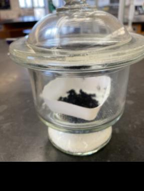
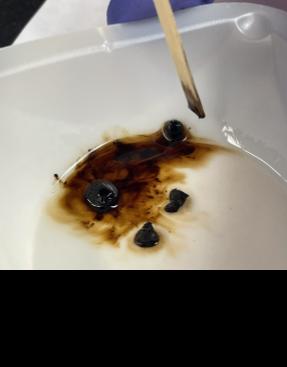
The resulting precipitate was then washed 3 times with distilled water. In each of the washings, a magnet was held to the bottom of the beaker to collect the magnetite before the water was poured off. This also helps to reduce the amount of low quality magnetite that is not

able to stick to the magnet. Three washings in 90% isopropyl alcohol were then performed to destroy any oleic acid that was not coating the magnetite. The powder was then dried with drierite, a desiccating salt composed of anhydrous calcium sulfate, desiccator for 48h. Drierite is also coated in cobalt chloride, which changes from blue to pink as water is absorbed.

Due to initial difficulties in making ferrofluid with the scaled down procedure, a batch following the reference exactly was created. Because the large batch resulted in much more magnetite than was needed for analysis, it was turned into a display. To do this, 3g of magnetite were put into a wayboat. Then 3g of kerosene was added. After this, the magnetite and kerosene were stirred together with a wooden splint until no more magnetite would disperse. Once the kerosene was saturated, it was pipetted out into a bottle full of distilled water.

RESULTS AND DISCUSSION

When originally attempting the synthesis, because of a lack of familiarity with the exact mechanism of coprecipitation, not enough ammonia was used. While stoichiometrically, 8 moles of ammonia hydroxide should be used for each mole of ferrous chloride, the solution needs to be at a pH above 9 for the ferrous oxide to begin to precipitate. This is made harder to observe because ferric oxide is able to precipitate at a pH of around 8 before quickly dissolving back into solution. Due to this lack of understanding, although stoichiometrically enough ammonia was used, magnetite was not able to precipitate and multiple attempts to produce ferrofluid failed. Because of this, another scientist attempted the exact procedure laid out and realized that a high pH is important for the precipitation of magnetite.

As well as being used for opacity measurements, some ferrofluid was stored in a bottle as a display. While in one batch the ferrofluid only stuck to the walls of the glass container where it contacted it before the water, when creating a larger display with the excess ferrofluid it stuck to the wall even after the distilled H2O was added. This was interesting to observe and showed how small changes in things like the glass used can cause large qualitative differences.

After the successful synthesis of magnetite nanoparticles coated in the oleic acid surfactant, the transparency of 1 g magnetite per 80g kerosene compared to around 1 to 1 used in commercial products. Even with this high of a dilution, only about 20% of visible light was transmitted, indicating just how opaque this solution is. This was measured with a model 721 spectrophotometer

ACKNOWLEDGMENTS

The author would like to acknowledge Mr Michael Sizer for his continued support and help troubleshooting the procedure.

The scientific results and conclusions and any views or opinions expressed herein are those of the author and do not necessarily reflect the views and policies of The Grayson School, Delaware County, or the US government and its agencies.

Funding: This experiment was supported by the Department of Science, The Grayson School.

Competing interests: The author declares no competing interests.

REFERENCES

1. Arrighi, Robert. “Novel Rocket Fuel Spawned Ferrofluid Industry.” NASA, 25 Feb. 2021, www.nasa.gov/history/novel-rocket-fuel-spawned-ferrofluid-industry/. Accessed 7 May 2025.

2 Minuti, Anca Emanuela, et al “Fe-Cr-Nb-B Ferrofluid for Biomedical Applications ” Nanomaterials, vol 12, no 9, Apr 2022, p 1488, https://doi org/10 3390/nano12091488 Accessed 7 May 2025

3. H. Chiriac, et al. “Fe-Cr-Nb-B Ferromagnetic Particles with Shape Anisotropy for Cancer Cell Destruction by Magneto-Mechanical Actuation ” Scientific Reports, vol 8, no 1, Nature Portfolio, July 2018, https://doi org/10 1038/s41598-018-30034-3 Accessed 7 May 2025

4. Socoliuc, V., et al. “Ferrofluids and Bio-Ferrofluids: Looking Back and Stepping Forward.” Nanoscale, vol. 14, no 13, 2022, https://doi org/10 1039/d1nr05841j Accessed 7 May 2025

5 Hackster io “OpenDLS, an Open-Source Dynamic Light Scattering ” Hackster io, Hackster, 3 July 2019, www.hackster.io/etienner/opendls-an-open-source-dynamic-light-scattering-bff60f. Accessed 7 May 2025.

6 Li, Jian “The Increase of the Light Transparency Induced by a Magnetic Field for the Colloid Film Based on α–FeOOH Nanoparticles ” Optica org, 2025, opg.optica.org/ome/fulltext.cfm?uri=ome-2-12-1760&id=245431. Accessed 7 May 2025.

7. Oehlsen, Oscar, et al. “Approaches on Ferrofluid Synthesis and Applications: Current Status and Future Perspectives ” ACS Omega, vol 7, no 4, Jan 2022, pp 3134–50, https://doi org/10 1021/acsomega 1c05631 Accessed 7 May 2025

8. Park, Jongnam, et al. “Ultra-Large-Scale Syntheses of Monodisperse Nanocrystals.” Nature Materials, vol. 3, Nov 2004, pp 891–95, https://doi org/10 1038/nmat1251 Accessed 7 May 2025

9 Sanz-Felipe, Ángel, et al “Optical Transmission of Ferrofluids Exposed to a Magnetic Field: Analysis by Electromagnetic Wave Propagation Numerical Methods.” Journal of Molecular Liquids, vol. 315, Oct. 2020, p 113713, https://doi org/10 1016/j molliq 2020 113713 Accessed 7 May 2025

10 Yerin, Constantine V , and Victoria I Vivchar “Effect of a Magnetic Field on the Transmission Spectra of Magnetic Fluids with Different Sizes of Nanoparticles.” Journal of Magnetism and Magnetic Materials, vol. 595, no. 171437, North-Holland, Oct. 2023, https://doi.org/10.1016/j.jmmm.2023.171437. Accessed 7 May 2025

Synthesizing benzyl acetate, butyl acetate, and isoamyl acetate using Fischer esterification

1*☨

Beesan Muaddi

ABSTRACT

Benzyl acetate, n-butyl acetate, and isoamyl acetate were synthesized in this study via fischer esterification, both in small samples in-vial and larger samples using a reflux apparatus. Purification of esters were performed using sodium bicarbonate for acid neutralization, anhydrous salt dehydration, and distillation. Isoamyl acetate yielded the clearest product, resulting in a pale yellow liquid with a banana-like scent. N-butyl acetate and benzyl acetate presented more complications.

INTRODUCTION

Esters are organic compounds that fall under the carbonyl category (Fig. 1A) A carbonyl is an organic molecule that contains a double bonded oxygen. Esters contain this double bonded oxygen in addition to an alkoxy group adjacent to the carbonyl portion. Esters are used in a wide variety of products, including but not limited to food flavorings, cosmetics, essential oils, and perfumes [1]. They can be naturally produced or synthesized generally by reacting an alcohol with another organic molecule, typically carboxylic acids, acid anhydrides or acid chlorides [2] They are naturally found in fats, oils, fruits, flowers as well as some biological molecules like pheromones. (Fig. 1B-D).

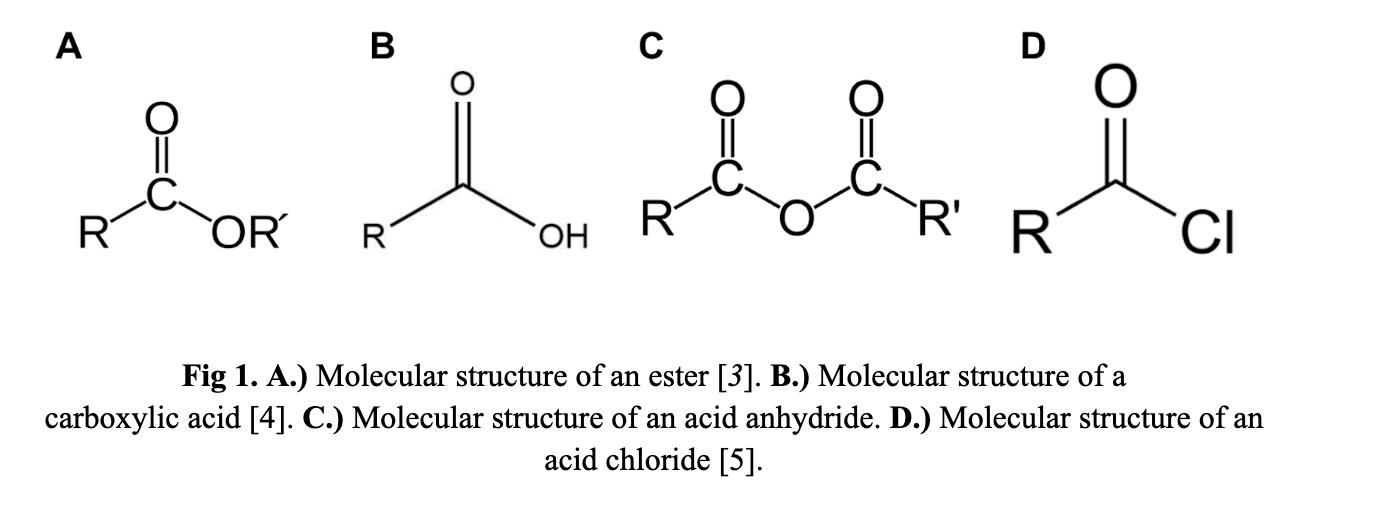
1Department of Science, Class of 2026, The Grayson School, Radnor PA.

2Department of Science, Class of 2026, The Grayson School, Radnor PA.

*Lead author of this work

☨ Corresponding author: bmuaddi@thegraysonschool.org

Muaddi, Scientific Transactions of the Grayson Society, May 2025

The term “ester” was coined by a German chemist, Leopold Gmelin, who discovered esters in 1848. The name is likely derived from the German word Essigäther, meaning acetic ether.

German chemist, Leopold Gmelin, discovered and named esters in 1848, likely derived from the German word Essigäther, meaning acetic ether. [6] However, the modern understanding of ester ’s structure and synthesis was not understood until 1895 when Emil Fischer discovered Fischer esterification. Fischer esterification uses a mixture of carboxylic acids and alcohols to produce esters. [7]

The general mechanism that esterification follows has 5 steps. First, the carbocation intermediate is formed: the electron from the oxygen’s pi bond in the carbonyl forms a bond with the hydrogen ion in the catalyst (Fig. 2A). A carbocation is a molecule containing a positively charged carbon atom, it is typically found as an intermediate stage in organic reactions. Then, the oxygen in the alcohol creates a bond with the carbocation (Fig. 2B) The oxygen in the alcohol becomes positive, and the hydrogen bonded to it transfers to another hydroxyl group to form a good leaving group, H2O (Fig. 2C) The pi bond is formed by eliminating the leaving group and the catalyst bonds with the hydrogen that is attached to the double bonded oxygen (Fig. 2D-E) This results in the formation of the ester, and water It is important to note that this reaction is reversible. In the presence of water, esters hydrolyze and break down into its alcohol and carboxylic acid components. If the ester is to be preserved it is essential that it is dehydrated [2].

Dehydration can be done in a number of ways. The methods attempted in this study were using anhydrous salts and distillation. Calcium chloride was used as the anhydrous salt for dehydration.

Esters synthesized in this study include n-butyl acetate, benzyl acetate, and isoamyl acetate. Specific uses for n-butyl acetate include a solvent for lacquers, paints, pharmaceuticals, and adhesives. It is also used as an artificial flavor in pharmaceuticals as well as a scent in cosmetic products. N-butyl acetate is a transparent liquid that smells like pear or apple, much like ethoxy ethyl acetate, but due to n-butyl acetate’s low toxicity and environmental impacts, it is more commonly used [8]. Benzyl acetate is an oily, colorless, liquid that is typically used for soaps and essential oils. It can be naturally found in jasmine, ylang-ylang, tobira, and other flowers [9]. Isoamyl acetate is a translucent yellow liquid that has a fruity banana-like fragrance. It is commonly used in foods and

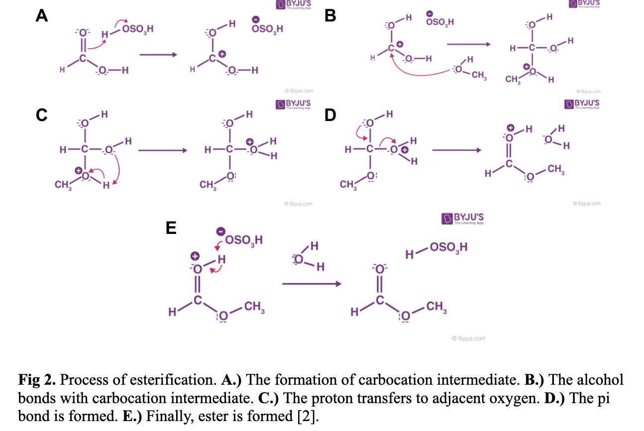
drinks such as honey, butterscotch, artificial coffee, as well as perfumes [9].

MATERIALS AND METHODS

Using Fischer esterification, synthesis and purification of isoamyl acetate, n-butyl acetate, and benzyl acetate were attempted.

There were 4 samples synthesized, each in 4.5 mL vials with seals. The first sample contained 1.2 mL of isoamyl alcohol and 2.5 mL of glacial acetic acid. Two vials contained 1 mL of n-butyl alcohol and 1.5 mL of acetic acid. The last vial contained 1 mL of benzyl alcohol and 1.5 mL of acetic acid. Then, 5 drops, approximately half of a milliliter, of sulfuric acid was added to each vial. All of the vials were sealed and placed in boiling water, heated by an immersion heater. (Fig. 3) The isoamyl acetate mixture was heated for 25 minutes, the n-butyl acetate mixture was heated for 30 minutes and the benzyl acetate mixture was heated for 31 minutes. Vials were removed from the hot bath for a minute before being placed into an ice bath for 3 minutes. [11]

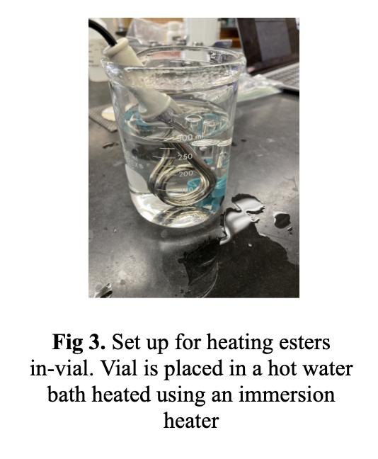
To purify the ester, contents of each of the vials were transferred to test tubes containing ice water. The organic layers were transferred back into the synthesis vials. 2 ml of saturated sodium bicarbonate solution was slowly added to the vials. This is done to neutralize any excess acetic acid or sulfuric acid. The aqueous layer was then removed. This process was completed twice. Finally, distilled water was added to the vial then removed to wash the ester.

A boiling point test was performed on the isoamyl acetate sample to assess the purity of the ester. The isoamyl acetate was transferred to a test tube and it was connected to a thermometer using a rubber band. A capillary tube was placed, open side facing down, into the test tube containing the ester. The thermometer and test tube were placed in the thiele tube containing silicone oil. The thiele tube was then heated until the temperature reached above the expected boiling point of isoamyl acetate. The sample was then allowed to cool. Once the sample began to fill the capillary tube, that was the temperature recorded as the boiling point (Fig. 4) [12].

Synthesis of n-butyl acetate and benzyl acetate was then performed using a reflux apparatus. For the n-butyl acetate sample, 10 ml of n-butyl alcohol and 12 ml of acetic acid and 15 drops of concentrated sulfuric acid were added to

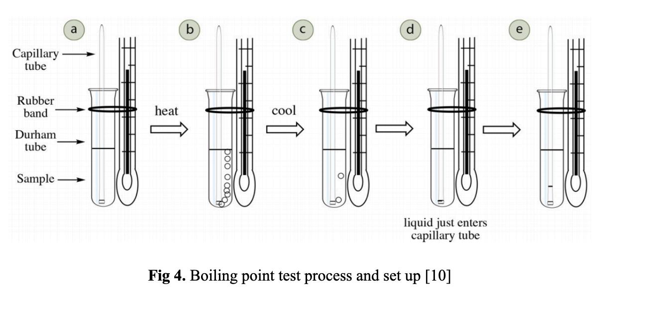
a round bottom flask. For the benzyl acetate sample, 10 ml of benzyl alcohol and 30 ml of acetic acid with only 5 drops of sulfuric acid were added to a round bottom flask. A reflux condenser was connected to the flask, then it was placed in a boiling water bath (Fig. 5) [13]. The n-butyl acetate mixture heated for 30 minutes, and the benzyl acetate mixture heated for 2 hours. After the mixture cooled, it was placed in a separatory funnel that contained a sodium carbonate solution composed of 15 ml of distilled water and roughly 4.5 g of solid sodium carbonate and carbon dioxide was produced. Once bubbling stopped, the separatory funnel was capped and shaken, to produce more carbon dioxide. It was then unsealed, to let out more carbon dioxide. This was repeated about 20-30 times, until all of the carbon dioxide was released. The separatory funnel was placed back on the ring stand and the bottom aqueous layer was discarded and the remaining organic layer was transferred to a flask and sealed. Then, each of the samples were washed with distilled water

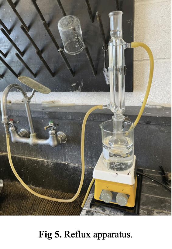
Calcium chloride was added as a drying agent to the esters and decanted to further purify the samples, ridding them of any remaining water [14].

Finally, a distillation was performed on n-butyl acetate. The apparatus included a hot sand bath in which a round bottom flask containing approximately 12 ml of n-butyl acetate and boiling stones was inserted. A thermometer was inserted above the round bottom flask. Additionally, a condenser is attached, with a receiving flask at the end. (Fig. 6) It is critical to note that the round bottom flask that is heated should never be heated to dryness. This is because high-boiling explosive compounds may be present, possibly resulting in an explosion or damage of glassware. The material left in the flask is called the “holdup.” [15]

RESULTS

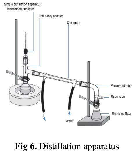
For the 4 samples synthesized in the vials, results varied. The isoamyl acetate sample turned black and cloudy in the hot water bath. The butyl acetate sample remained clear For the benzyl acetate sample, when the sulfuric acid was added, a red precipitate formed. The precipitate turned white and solidified at the bottom of the vial. After one day, the precipitate turned into a gel (Fig. 7)

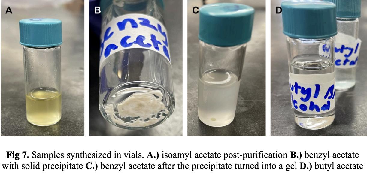
Despite some of the unanticipated results, the purification process was still performed on all samples. Once purified, the isoamyl acetate sample became a translucent yellow color and smelled like banana (Fig. 7A). The butyl acetate sample failed to form a meniscus, therefore the organic layer was not isolated. When the purification process was performed on the benzyl acetate sample, it was too difficult to distinguish between the precipitate, organic layer, and aqueous layer. The benzyl and butyl acetate samples were discarded. Additionally, the aroma for both butyl and benzyl acetate did not smell fruity or floral. For this reason, only isoamyl acetate had the boiling point test performed to assess the purity. The boiling point of isoamyl acetate is 142°C, the sample synthesized had a boiling point of 140°C.

The butyl acetate that was synthesized using a reflux apparatus yielded far more product than the butyl acetate synthesized in the vials. When heated, the sample remained clear When the butyl acetate was added to the sodium carbonate solution, it created a considerable amount of CO2 bubbles. Once the bubbles stopped, there were two menisci, leaving 3 layers (Fig. 8A) Once the incremental shaking and releasing of CO2 was performed, there was only 1 meniscus (Fig. 8B) Once purified, the butyl acetate was a pale yellow color and smelled floral and fruity

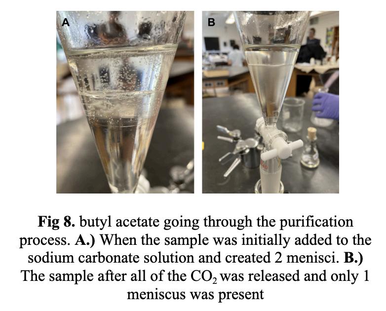
The benzyl acetate synthesized using the reflux apparatus worked. The precipitate still formed, but after heating it seemed to have disappeared. When the distillation was performed, the boiling point of n-butyl acetate, 117°C, was not reached. However, the liquid in the receiving flask was clear and still smelled like n-butyl acetate, suggesting that the n-butyl acetate was purified.

DISCUSSION

The in-vial synthesized butyl acetate failed to form a meniscus, this is likely due to the extremely small yield. Therefore, the synthesis was repeated, increasing the reactants by tenfold, which resulted in a greater yield.

The precipitate created by the benzyl acetate is likely the sulfuric acid polymerizing the benzenes. In the end, the desired result was achieved, so it seems that this side reaction is negligible. When the ester was being washed with water it failed to form a meniscus, due to how similar the density is to water (Fig. 9) Adding salt to the water to change the density is a simple fix to this issue.

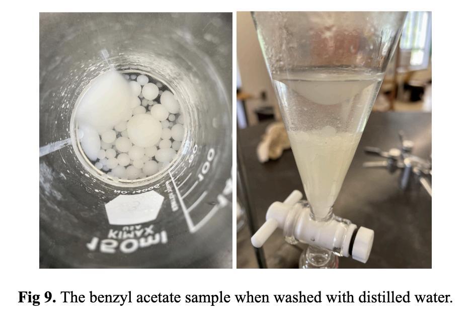
The isoamyl acetate, although not going through the anhydrous salt dehydration still proved to be relatively pure with the boiling point varying by 2 degrees.

When distillation of n-butyl acetate was performed, the temperature rose approximately 10-20 degrees, then dropped 5-15 degrees repeatedly. This likely occurred due to the lower boiling point components distilling, requiring more heat to distill the higher boiling point components. [15]

ACKNOWLEDGMENTS

We would like to thank Consolidated Chemical & Solvents LLC for providing the materials used during this experiment. We thank M. Sizer and classmates for their feedback on analysis and interpretation. The scientific results and conclusions and any views or opinions expressed herein are those of the authors and do not necessarily reflect the views and policies of the Grayson School, Delaware County, or the US government and its agencies. Funding: This experiment was supported by the Department of Science, The Grayson School. Competing interests: The authors declare no competing interests. License information: Copyright Ⓒ 2023 the authors.

REFERENCES

1. “Ester.” BYJU'S, BYJU'S, https://byjus.com/chemistry/ester/. Accessed May 2025.

2 “Esterification ” BYJU'S, https://byjus.com/chemistry/esterification/#:~:text=5:%20Ester%20formation-,Esterification%20Methods,F rom%20carboxylic%20acid%20and%20alcohol Accessed May 2025

3. Helmenstine, Anne Marie. “What Is an Ester in Chemistry?” ThoughtCo, 4 January 2020, https://www thoughtco com/definition-of-ester-605106 Accessed 7 May 2025

4. Fisch, Kyle. “Naming Carboxylic Acids.” Study.com, https://study com/skill/learn/naming-carboxylic-acids-explanation html Accessed May 2025

Muaddi, Scientific Transactions of the Grayson Society, May 2025

5 Reid, Danielle “Acid Chloride | Uses, Formation & Reaction ” Study com, https://study com/academy/lesson/acid-chloride-formation-reaction html Accessed 7 May 2025

6 “Functional Groups Names, Properties, and Reactions – Introductory Chemistry ” UEN Digital Press with Pressbooks, https://uen pressbooks pub/introductorychemistry/chapter/functional-groups-names-properties-and-reaction s/ Accessed 27 May 2025

7 Carboxylic Acids to Esters: Acid-Catalyzed (Fischer) Esterification Overview https://www jove com/science-education/v/12348/carboxylic-acids-to-esters-acid-catalyzed-fischer-esterific ation#:~:text=April%2030%2C%202023-,Overview,drive%20the%20reaction%20to%20completion.

8 Liu, Kun “Separation of organic compounds from water by pervaporation in the production of n-butyl acetate via esterification by reactive distillation.” Science Direct, 2005, https://www sciencedirect com/science/article/abs/pii/S0376738805001638 Accessed May 2025

9. Hongjie, Lu. “AN OVERVIEW ON SYNTHETIC METHODS OF BENZYL ACETATE.” European Chemical Bulletin, 2013, https://epa.hu/02200/02286/00015/pdf/EPA02286 European Chemical Bulletin 2013 05 272-274.pdf. Accessed May 2025

10. Torres, Sebastian. “Banana flavor: insights into isoamyl acetate production.” https://epa hu/02200/02286/00015/pdf/EPA02286 European Chemical Bulletin 2013 05 272-274 pdf Accessed May 2025.

11 McPherson “GRANULAR CALCIUM CHLORIDE AS A DRYING AGENT ” ACS Publications, 1917, https://pubs.acs.org/doi/pdf/10.1021/ja02252a004. Accessed May 2025.

12 Flinn Scientific “Vial Organic™ Ester Lab ” Accessed 2025

13. Flinn Scientific. “How to Use a Thiele-Dennis Tube.” https://www flinnsci com/api/library/Download/46b1e79b05414c7f8e4164d9df5215ff?srsltid=AfmBOoqPd CkdwdqloRtgqitNsr9CHMnhILJ8iRb7u1isLZ2-jIf5Cz-E.

14 Thermo Scientific “Fisher Esterification Synthesis of Isopentyl Acetate (Banana oil): picoSpin 45 ” Thermo Scientific. Accessed 2025.

15 Nichols, Lisa “7 19: Using Drying Agents ” Chemistry LibreTexts, 7 April 2022, https://chem libretexts org/Bookshelves/Organic Chemistry/Organic Chemistry Lab Techniques (Nichols )/07%3A Technique Summaries/7 19%3A Using Drying Agents Accessed 7 May 2025

16 Distillation1 UNIVERSITY OF MASSACHUSETTS AMHERST pdf

POSTER:

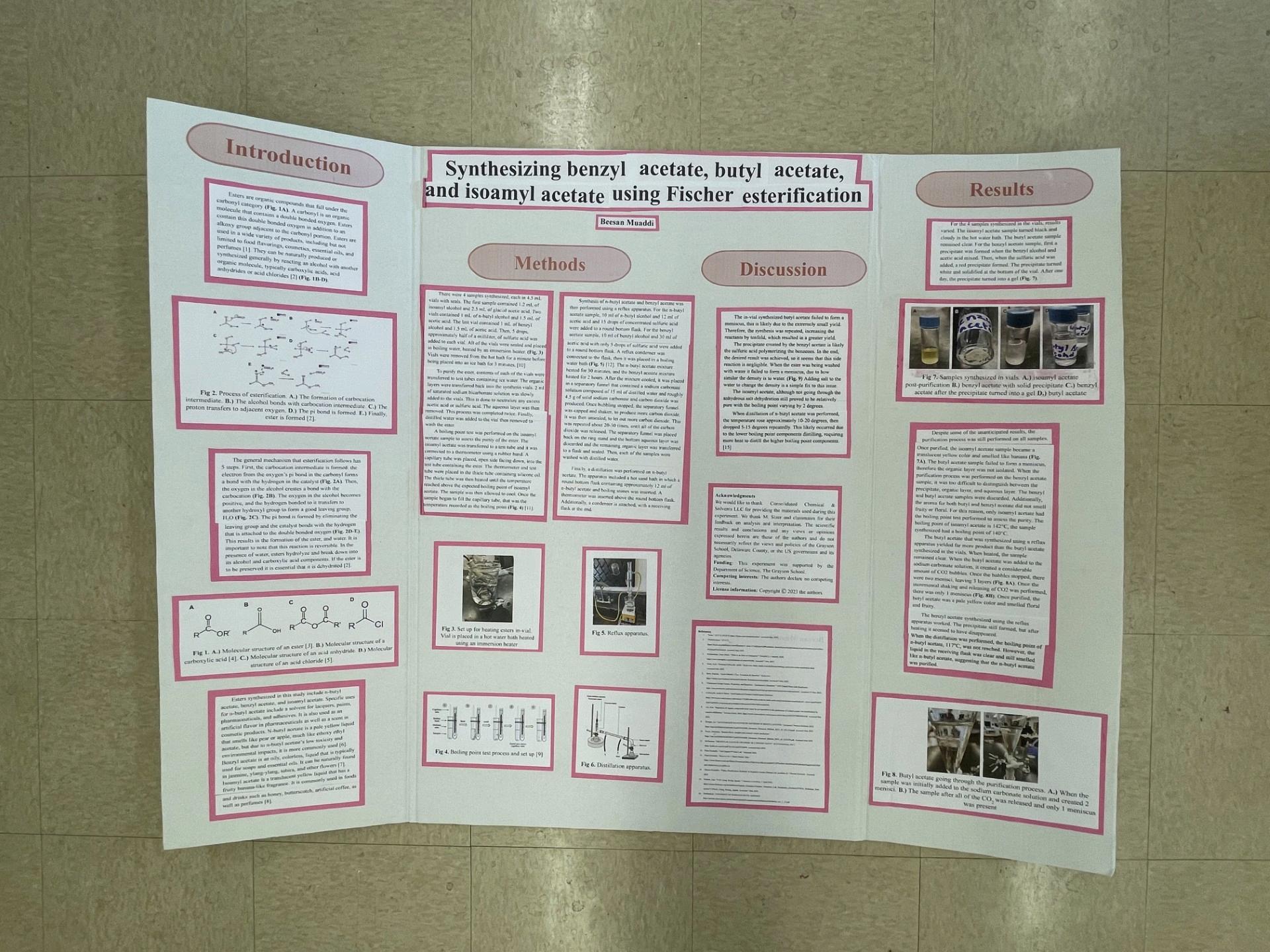
Tracking the spread of a simulated disease through a school using an enzyme-linked

immunosorbent assay

Beatrix Lay1

ABSTRACT

Throughout the 50+ years since its discovery, the enzyme-linked immunosorbent assay (ELISA) has been adapted for numerous scientific processes, but none have been proven to be as important as ELISA testing for viral antigens. In this experiment, a disease-spreading simulation was performed using g-immunoglobin (IgG) from chickens, with one participant given a positive sample. The antigen was “spread” between participants in controlled rounds and all sharing partners were recorded. An ELISA was run on all samples, and all participants who were predicted to yield a positive result presented a positive result. This study confirmed previous findings about the efficacy of ELISA to detect viral antigens and measure the spread of a disease.

INTRODUCTION

There has hardly been a technical innovation which has affected the field of epidemiology more than enzyme-linked immunosorbent assays. The ELISA method was developed in 1971 by Eva Engvall and Peter Perlmann as a way of testing for either the presence or the concentration of certain biological substances. As our understanding of microbiology grew in the 20th century, scientists like Engvall and Perlmann explored the relationship between antibodies and antigens as a route to further the study of epidemiology The antibody—a protein that is a vital part of the human body’s immune defense—is a near-surefire way of detecting if a person has encountered the antigen—a substance foreign to the body—in question, due to their fundamentally correlative nature (Figure 1) (1).

Prior to the development of ELISAs, testing for the presence of an antigen or antibody had to be achieved by performing radioimmunoassays. Radioimmunoassays (RIA) are a way to read antibody/antigen interactions using a radioactive isotope, commonly iodine-125 (2). The radioactive isotope is bound to the known antigen, and the patient’s antibodies bind with the antigen, therefore once the radioactive substrate is added the ratio of unbound antibodies can be analyzed (3). The initial discovery was made with insulin as the antigen, but soon it was seen how useful RIAs really were, as they enabled all sorts of drug, cancer, and other biological research

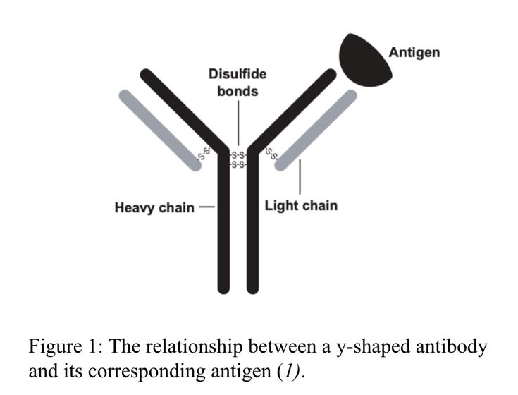
1 Department of Science, Class of 2025, The Grayson School, Radnor, PA Lay, Scientific Transactions of the Grayson Society, May 2025

(4). The downside, however, was that RIAs were expensive (synthesizing radioisotopes must be done with a nuclear reactor) and hard to safely run and dispose of (the half lives of the isotopes can be very short, meaning tests are hard to repeat if necessary). Scientists were looking for a way to test the same biological substances with a similar sensitivity but much cheaper and safer (5). This is when Engvall and Perlmann discovered the ELISA technique.

The fundamental difference between the ELISA and the RIA is the elimination of the radioactive isotope to tag the antibodies with a specialized enzyme instead of a radioisotope (6). In Engvall and Perlmann’s historic 1971 experiment, the antigen used was Immunoglobin G (IgG) from a rabbit (7). Next, matching antibodies with the enzyme indicators (most commonly horseradish peroxidase (HRP) and alkaline phosphatase (AP)) were loaded into the wells (8). If the targeted antigen was present in the initial sample, the antibodies would bind, whereas if the sample did not contain the antigen in question, then the antibodies would get washed out during the washing step. The final addition to their ELISA procedure is the substrate, which is a solution that produces a visual change in wells containing the antigen. In 2012, however, de la Rica et. al. discovered a way to use gold nanoparticles at very low concentrations that can be read by a machine so that the tests can provide not only qualitative, but also quantitative results, as in the case of checkerboard or sensitivity analysis (9). The method as described by Engvall and Perlmann was what is now referred to as a direct ELISA (figure 2). In a direct ELISA, the antigen is loaded into the wells of a microtiter plate and is let to bind during incubation before getting washed out.

Apart from direct ELISA, there are two other common ways to run an ELISA test. The indirect method simply requires both a primary and secondary antibody and is typically used when the primary antibody is harder to come by/poses issues when attached with the enzyme, and so an additional antibody is added for ease of use (10). A sandwich ELISA also uses two different antibodies, but instead of the antigen getting added to the wells first, one of the antibodies is bound to the plate, then the antigen, and lastly the second antibody (6). This type of test is the most sensitive, but also the most time consuming and expensive. Over the years, these variations on ELISA have been developed as needed to adjust all of the variables that can make the tests as accurate and specific for each application (11).

ELISA is used in labs for a myriad of purposes, including but not limited to: viral antigen testing, pregnancy testing, drug testing, GMO testing in plants, detecting toxins/contaminants in waterways or the environment, blood testing for diseases, checking vaccine status, cancer screenings, and allergy testing (1). Since the discovery of ELISA in 1971, the process has been adapted

Lay, Scientific Transactions of

Grayson Societ

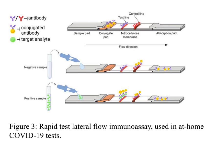
numerous times for a number of biological processes. While normally performed in a “wet lab” setting, scientists have adapted a “dry-lab” technique from the ELISA process, known as a rapid test. Rapid antigen tests, like the one in Figure 3, work similarly by collecting a sample and mixing the sample into a solution, then letting the solution run through a paper loaded with two regions of antibodies with indicator (12)(13).

Of all the applications for ELISA tests, some of the most important ones in recent memory are rapid tests, famously used during the COVID-19 pandemic to provide quick reliable results and prevent spread of disease. Because of the easily adaptable framework of the tests, ELISA was also the first method to detect HIV in the 1980’s, which swiftly increased scientists and doctors ability to identify and treat the disease (14). The high sensitivity of ELISA is particularly important for diseases like HIV due to the low rate of false positives (15). Over the years, ELISA testing for viral antigens has evolved, and ELISA is still the primary test used to determine if a person has HIV and at-home COVID-19 tests are based on an immunoassay format (16).

For diseases which cause epidemics like HIV and COVID-19, tests such as ELISA are extremely useful not only in diagnosing patients, but also in finding the root causes of the diseases by understanding the vector in which people get infected. When AIDS was first discovered in 1981, people did not know that it was caused by HIV. It was only through studies such as Auerbach et. al. that researchers attempted to track the spread and could identify key characteristics of the disease (17). Without this sort of initial research of sexual partners (as in the case of HIV) or people who otherwise had contact with a known infected person, public health measures cannot be put in place and information cannot be spread about how to protect oneself or get treatment.

ELISA has played a vital role in quickly and accurately recognizing the presence of an antigen in the context of the AIDS and COVID-19 pandemics, but also in the greater picture of public health. In this experiment, we ran a disease simulation by inviting volunteers to the lab and having participants “spread” the disease by pipetting their samples into each other ’s vials. Each student exchanged their sample with others three times. One participant was given an infected sample which contained the antigen, while others became infected through the course of the simulation. An ELISA was then run on all samples in addition to positive and negative controls. The results were interpreted and compared to the predicted results based on the spreading simulation.

MATERIALS and METHODS

All antigens, antibodies, and other specific materials were obtained as part of the Biotechnology Explorer™ ELISA Immuno Explorer™ Kit from Bio-Rad.

In preparation to run the experiment, 90 ml of distilled water and 10mL of 10X Phosphate-Buffered Saline (PBS) were added to a bottle, making 1x PBS solution. The wash

buffer was made by combining 805mL distilled water, 90 mL of 10X PBS buffer and 4.5 mL 10% Tween 20. The antigen, primary antibody and secondary antibodies were rehydrated by adding 0.5 mL of 1X PBS solution to each vial; all three vials were then closed and shook for 5 seconds until mixed. To dilute the antigen, 150 µL of 50X antigen and 7.5 mL 1X PBS were added to a bottle and mixed before being labelled 1X Ag. Next, 24.5 mL of wash buffer and 0.5 mL of primary antibody were added to a bottle, shaken, and labeled 1X PA. This step was repeated with the secondary antibody and labeled 1X SA. Then, 14 yellow tubes were labeled #1-14 to be used as the samples. Tube #7 (the positive sample) had 650 µL of 1X PBS and 100 µL of 50X AG were added. All other tubes were filled with 750 µL of 1X PBS. The sample tubes and all other reagents were closed and placed in a 4° C fridge for a week.

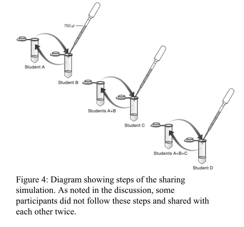
A week later, all the samples were taken out of the fridge. Fourteen participants were selected to participate in the “bodily fluid sharing” simulation (figure 4). Each participant was given a microcentrifuge tube filled with one of the samples labeled #1-14 and a pipet. Each round of swapping consisted of participants pairing up, emptying the contents of one sample into the other, mixing gently with the pipet, and taking half of the sample back into the other tube. Three rounds of swaps ensued, with participants asked to record who they swapped with in each round. Participants were instructed to swap with different people each time, yet due to a mistake one pair of participants swapped with each other in both rounds one and three. This concluded the disease sharing simulation.

Each 12-well microtiter strip was labeled with three plus signs “+” for positive controls, three minus signs “-” for negative controls, and two numbered samples, each in triplicate (for example, the strip with samples five and six would have read “+++---555666”). Once labeled, 50µL of the positive control were added to all wells marked “+” in increments of two 20µL measurements and one 10µL measurement. Next 50µL of the negative control were added to all wells marked “-” in the same increments. 50µL of each numbered sample were added to the wells with the corresponding number. Pipet tips were changed when a new substance was added, or periodically to prevent contamination. Once all substances had bound to the wells, the washing step began. Each strip was removed from the tray and gently tapped out onto a dry paper towel to remove all excess liquid. A couple drops of wash buffer were carefully added to each well before the wells were turned over once again onto a dry paper towel. This process was repeated twice for each strip.

After washing, 50µL of primary antibody was added to every well, once again in increments of two 20µL measurements and one 10µL measurement. Pipet tips were changed only with discretion when contamination could have occurred. After the incubation period, the washing process was repeated for the primary antibody with each strip getting washed twice. Once the wells were washed, 50µL of secondary antibody was then added to all wells in the same increments. Pipet tips were also changed only when contamination could have occurred. After a similar incubation period, the washing process was repeated for the secondary antibody.

To conclude the ELISA, 60µL of HRP-enzyme substrate was added to all wells in three 20µL increments. Almost immediately all positive wells began to change color and after letting the strips sit for 1-2 minutes, photos were taken, and results were recorded.

RESULTS

Figure 6 shows the results of the ELISA 3-5 minutes after the substrate was added. All positive controls were bright blue, and all negative controls were clear, indicating no visible contamination. Samples 1, 2, 3, 5, 7, 9, 10, 11, 13, and 14 were positive. All samples that were predicted to be infected, as seen in Figure 7, did turn out to be positive. The progression of infection is shown in Figure 8, with each column indicating a “round” of sample swapping.

DISCUSSION

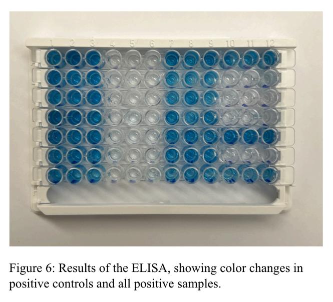
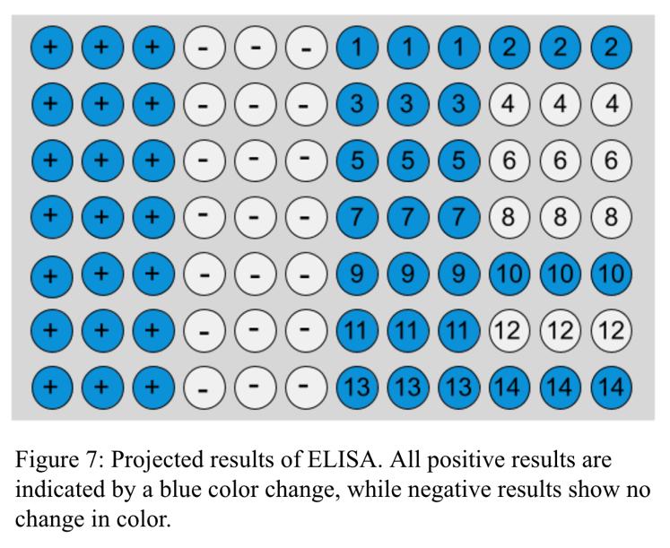
For a result to be interpreted as positive, that is, containing the antigen, we were looking for a blue color change. In samples that turned blue (1, 2, 3, 5, 7, 9, 10, 11, 13, 14; all positive controls) this means the antigen, γ-Immunoglobin, bound to the microtiter wells. This means when the primary antibody was added, the primary antibody bound to the antigen, as it does in the body when fighting an infection. The HRP-linked secondary antibody was then able to bind to the primary antibody in wells with the antigen. Therefore, when the substrate was added all

the necessary parts of the framework were there and the color of the well changed. In all samples that stayed clear, no detectable amount of antigen was present in the initial samples (non-infected participant samples, negative controls) and no detectable contamination occurred during the procedure.

A slight error occurred during the sharing simulation. The directions dictated clearly delineating between each round so that each participant was trading with someone else also on that same round as them.

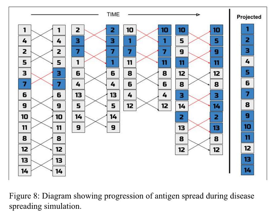
Samples 8, 10, 11 and 12 did not trade within the second round (second column), meaning that they made their second trade while their partners were making their third trade. This extra "mini-round" generated two more positive samples than the algorithm (if done correctly) should generate, since the amount of positive samples per round should theoretically only double. This mistake had no significant effect on the outcome other than producing a higher-than-anticipated number of positive results. Had people’s trading partners not been written down, it would have been much harder to track the spread of disease. Doctors rely on this sort of documentation to track diseases, such as HIV.

Another variation occurred between the instructions and the actual procedure. The directions dictate to let each well sit with the proteins for five minutes. An intentional choice was made to not time each step, because these directions had in mind that someone was only working on one strip at a time. Instead, each step was completed over the whole tray left to right, top to bottom, and the next step would immediately follow In many cases, these steps took well over five minutes to complete.

This study confirmed that ELISA is a highly sensitive and effective way to both detect antigens and track the spread of disease. Scientists can continue to rely on ELISA to accurately diagnose people with viral diseases. While assays using a sample with a high viral load, like this one, often yield accurate and precise results, developments could be made to improve the result accuracy for samples with lower viral loads, for example, right after a person was exposed.

REFERENCES

1. Bio-Rad. "Biotechnology Explorer™ ELISA Immuno Explorer™ Kit." n.d. Instruction Manual.

2. Harvard Department of Environmental Health and Safety. "Radioimmunoassay with Iodine 125: Standard Operating Procedure." Harvard University, n.d. Lab procedure.

3 Yalow, Rosalyn S and Solomon A Berson "General principles of radioimmunoassay " Clinica Chimica Acta (1968): 51-69

4 Craer, Jennifer R Radioimmunoassay: Embryo Project Encyclopedia 11 October 2013 7 May 2025

5 Taylor, F G , D Patel and F J Bourne "Comparison of sensitivities of ELISA and radioimmunoassay for detection of class-specific antibody in mouse serum" Journal of Immunological Methods (1983): 65-73

6. Alhajj, Mandy, Muhammad Zubair and Aisha Farhana. Enzyme-Linked Immunosorbent Assay. 23 April 2023. E-Book.

7. Engvall, Eva and Peter Perlmann. "Enzyme-linked immunosorbent assay (ELISA) quantitative assay of immunoglobin G " Immunochemistry (1971): 871-874

8 ThermoFisher Scientific ELISA Enzyme Substrates 2025 7 May 2025

9 de la Rica, Roberto and Molly M Stevens "Plasmonic ELISA for the ultrasensitive detection of disease biomarkers with the naked eye " Nature Nanotechnology (2012): 821-824

10 ThermoFisher Scientific ELISA technical guide and protocols n d Document

11 Fields, H A , et al "Experimental conditions affecting the sensitivity of enzyme-linked immunosorbent assay (ELISA) for detection of hepatitis B surface antigen (HBsAg) . " Bulletin of the World Health Organization (1983): 135-142.

12. National Institute of Health. Rapid Tests. 4 September 2024. 7 May 2025.

13 Mirica, Andreea-Cristina, et al "Latest Trends in Lateral Flow Immunoassay (LFIA) Detection Labels and Conjugate Process " Frontiers in Bioengineering and Biotechnology (2022)

14 Alexander, Thomas S "Human Immunodeficiency Virus Diagnostic Testing: 30 Years of Evolution " Clinical and Vaccine Immunology (2016): 249-253

15 Stanford Health Care Enzyme-Linked Immunosorbent Assay (ELISA) 2025 7 May 2025

16. Center for Disease Control. Getting Tested for HIV. 2024. 7 May 2025.

17. Auerbach, David M., et al. "Cluster of cases of the acquired immune deficiency syndrome: Patients linked by sexual contact." The American Journal of Medicine (1984): 487-492.

ACKNOWLEDGMENTS

The author would like to thank Bio-Rad for providing materials and the procedure used in this lab. Many thanks to M. Sizer for his assistance and support in preparing to run and executing the lab, and to N. Freidenreich for help during the procedure. The author would also like to thank all 12 volunteers from The Grayson School who participated in the sharing simulation. The results and any opinions expressed herein are those of the author and do not necessarily reflect the views or opinions of The Grayson School.

Funding: The materials in this experiment were funded by the Department of Science at The Grayson School.

Competing interests: The author declares no competing interests.

License Information: Copyright © 2025 the author.