
Sample Read

© All rights reserved
Price : ` 895
First Published : July 2026
Published by :
Taxmann Publications (P.) Ltd.
Sales & Marketing : 59/32, New Rohtak Road, New Delhi-110 005 India
Phone : +91-11-45562222
Website : www.taxmann.com
E-mail : sales@taxmann.com
Regd. Office : 21/35, West Punjabi Bagh, New Delhi-110 026 India
Printed at :
Tan Prints (India) Pvt. Ltd.
44 Km. Mile Stone, National Highway, Rohtak Road Village Rohad, Distt. Jhajjar (Haryana) India
E-mail : sales@tanprints.com
Disclaimer
Every effort has been made to avoid errors or omissions in this publication. In spite of this, errors may creep in. Any mistake, error or discrepancy noted may be brought to our notice which shall be taken care of in the next edition. It is notified that neither the publisher nor the author or seller will be responsible for any damage or loss of action to any one, of any kind, in any manner, therefrom.
No part of this book may be reproduced or copied in any form or by any means [graphic, electronic or mechanical, including photocopying, recording, taping, or information retrieval systems] or reproduced on any disc, tape, perforated media or other information storage device, etc., without the written permission of the publishers. Breach of this condition is liable for legal action.
For binding mistake, misprints or for missing pages, etc., the publisher’s liability is limited to replacement within seven days of purchase by similar edition. All expenses in this connection are to be borne by the purchaser. All disputes are subject to Delhi jurisdiction only.
Preface v Syllabus vii
UNIT I
MATRICES AND DETERMINANTS
Chapter 1: Matrices and Matrix Algebra
1.1 Introduction to Matrices1.3
1.1.1 Order of Matrix − Rows × Columns1.3
1.2 Types of Matrices1.4
1.2.1 Rectangular Matrix1.4
1.2.2 Square Matrix1.4
1.2.3 Triangular Matrix1.4
1.2.4 Diagonal Matrix1.5
1.2.5 Identity Matrix1.5
1.2.6 Scalar Matrix1.5
1.2.7 Null (or Zero) Matrix1.5
1.2.8 Symmetric Matrix1.5
1.2.9 Vector1.6
1.3 Algebra of Matrices1.6
1.3.1 Matrix Equality1.6
1.3.2 Matrix Addition1.6
1.3.3 Matrix Subtraction1.8
1.3.4 Matrix Multiplication1.8
1.3.5 Integral Power of Square Matrix1.10
1.4 Determinants, Minors and Cofactors1.10
1.4.1 Determinant of a 2 × 2 Square Matrix 1.10
1.4.2 Minors and Cofactors1.11
1.4.3 Determinant of a 3 × 3 square matrix 1.12
Chapter 2: Application of Matrices to Business and Economics
Chapter
3.1
3: Input-Output Analysis
Chapter 4:
Chapter 5: Application of
UNIT II
CALCULUS I
5.9
5.5.1
UNIT III
CALCULUS II
Chapter 8: Integration
UNIT IV
MATHEMATICS OF FINANCE
Chapter 10: Rates of Interest: Compounding and Discounting
UNIT V
LINEAR PROGRAMMING
Chapter 13: Simplex Method for LPP
Chapter 14:
UNIT VI
SPREADSHEET PRACTICALS
in Business

CHAPTER
Learning Objectives
By the end of this chapter, students will be able to:
Define matrices, classify their types, and perform basic matrix algebra.
Compute determinants, minors, cofactors, and find the transpose, adjoint and inverse of a matrix.
Express systems of linear equations in matrix form and solve them using the Matrix Inversion Method and Cramer’s Rule (Determinant Method).
Solve systems of linear equations using Gauss Elimination and Gauss-Jordan Elimination techniques.
1.1 INTRODUCTION TO MATRICES
A matrix is a collection of data arranged into a fixed number of rows and columns. Usually, the data consists of real numbers. In general, matrices can contain complex numbers, but they are not going to be used herein for an apparent application in business and eco-
nomics. Here is an example of a matrix with three rows and three columns: 243 71 54 386 . .
The top row that consists of data items {2, 4, 3} is row 1. The leftmost column that consists of data items {2, 7, 3} is column 1. This matrix is a 3 × 3 matrix because it has three rows and three columns. In describing matrices, the rows-by-columns format is used.
Each number that makes up a matrix is called an element of the matrix. These elements in a matrix have specific locations, identified by their respective row and column. The location of the element in the upper left corner of the matrix is row 1 and column 1. In the above matrix, the element in row 1 and column 1 has the value 2. The element in row 2 and column 3 has the value 5.4. A matrix (and its plural, matrices) in mathematics is a rectangular array of numbers, symbols, or expressions that are arranged in rows and columns. The individual items in a matrix are called elements or entries. The 3 by 3 matrix as given above is composed of 3 rows and 3 columns and consequently has 3 × 3 = 9 elements. Every matrix is named and denoted by a capital letter such as A, B, C … X, Y, Z.
1.4
Formally, a matrix is constituted by a set of m × n numbers that are arranged in the form of a rectangular array of m rows and n columns, as:
The first subscript m in an element. a mn of a matrix refers to the row number, and the second subscript n refers to the column number. It is important to remember this convention for performing matrix operations. Concisely, the above matrix is also denoted by A = []. aijmn Such a matrix is called an m by n matrix. If m = n, then the matrix is called a square matrix, as it will have the same number of rows and columns.
1.2 TYPES OF MATRICES
There are many types of matrices, each of which has distinctive properties. A few primary types of matrices are explained below.
A matrix that is formed by an unequal number of rows (m) and columns (n) is called a rectangular matrix, i.e., it has m ≠ n. For example, A = 32 26 59 is a 3 × 2 rectangular matrix
because the number of rows is not equal to the number of columns.
A matrix that is formed by an equal number of rows (m) and columns (n) is known as a square matrix, i.e., it has m=n. For example, A = 372 210 145 is a 3 × 3 square matrix because the number of rows (m) is equal to the number of columns (n).
A square matrix which has zero elements either above or below the principal diagonal is called a triangular matrix. Thus, there are two types of triangular matrices: (a) Upper triangular matrix and (b) Lower triangular matrix.
(a) Upper Triangular Matrix: A triangular matrix in which all the elements below the principal diagonal are zero is called an upper triangular matrix. For example, A = 621 054 009 is an upper diagonal matrix because the elements below its principal diagonal are zero.
(b) Lower Triangular Matrix: A triangular matrix in which all the elements above the principal diagonal are zero is called a lower triangular matrix. For example,
A = 300 590 414 is a lower triangular matrix because the elements above its principal diagonal are zero. If all diagonal elements of a triangular matrix are zero, it is called strictly triangular.
A square matrix which has non-zero elements in the principal diagonal and zero elements above and below the principal diagonal is called a diagonal matrix. A diagonal matrix is both an upper and lower triangular matrix. Consider the following 3 × 3 matrix. A = 300 050 002 is a diagonal matrix because its principal diagonal has the elements {3, 5, 2} and the elements below and above this diagonal are zero. Therefore, it is a diagonal matrix.
1.2.5 Identity Matrix
A diagonal matrix, in which all the elements of the principal diagonal are unity (i.e., one), is known as an identity matrix. Such a matrix is denoted by I. For example, I = 100 010 001 is an identity matrix of the order 3 because all its diagonal elements are one, and the rest of the elements below and above its principal diagonal are zero.
A diagonal matrix in which all the elements of the principal diagonal are the same but neither zero nor unity is known as a scalar matrix. For example, A = 600 060 006 is a scalar matrix of the order 3 because it has all its diagonal elements the same, i.e., 6.
A null (or zero) matrix is one which has all its elements equal to zero. For example, A = 000 000 000 is a zero matrix of order 3 because it has all its elements equal to zero. A zero matrix is usually denoted by O.
A symmetric matrix is a square matrix in which aij = aji for all i and j, where i denotes the row number and j denotes the column number of an element. In the following example, matrix A is symmetric, whereas matrix B is not symmetric.
A = 915 162 527 and B = 914 262 517
1.2.9 Vector
A vector is a matrix that has only one row (called a row vector or row matrix) or one column (called a column vector or column matrix). For example, matrix A is a column vector, while matrix B is a row vector: A = 5 9 9 and B = [] 386
1.3 ALGEBRA OF MATRICES
A generalized algebra that deals with the operations and relations among matrices is called the algebra of matrices. It refers to a part of algebra that deals with the theory of matrices. In this section, certain algebraic operations on matrices, such as equality of matrices, addition of matrices, multiplication of a matrix by a scalar, and difference and multiplication of matrices, shall be explained.
Two matrices A and B are said to be equal, expressed as A = B, only if these matrices are of the same order and their corresponding elements are equal.
Example 1.1: Given that there are two matrices, A = xy xy 6 4 and B = 26 144 such that A = B. Find out the value of x and y.
Solution: Equality of the given matrices implies that corresponding elements of A and B, viz., x – y and 2 are equal, i.e., xy 2. Similarly, xy 14. Solving for the values of x and y, we get x 8 and y 6.
1.3.2 Matrix Addition
For any two matrices, A and B of the same order m × n, their addition, denoted by A + B, is obtained by adding the corresponding elements of A and B. For example, if A = 341 526 ; B = 484 373 , then A + B = 7125 899
1.3.2.1 Properties of Matrix Addition:
There are six important properties of matrix addition.
1. Commutative Property: If A and B are matrices of the same order, then A + B = B + A.
2. Associative Property: If A, B and C are matrices of the same order, then (A + B) + C = A + (B + C).
3. Additive Inverse Property: If there is a matrix A, then there exists another matrix (denoted by A), which is obtained by reversing the sign of every element of matrix A. This matrix is called the additive inverse of A. The sum of the matrix A and the additive inverse of A is a zero matrix i.e., A + (– A) = (– A) + A = O.
4. Additive Identity Property: If there is a matrix A (with real numbers) and another matrix O (with zero elements), of the same order, then A + O = O + A = A. The matrix O is called the additive identity of matrix A.
5. Distribution of Scalar Multiplication over Addition: If A and B are two matrices of the same order, and there is a scalar k, then k(A + B) = kA + kB.
6. Applicability of Cancellation Laws: If there are three matrices A, B and C of the same order so that A + C = B + C, then A = B, by cancelling C on both sides.
Example 1.2: You are given the following 3 by 2 matrices:
Demonstrate the properties of matrix addition.
Solution:
(i) Commutative property: A + B = 54 69 414 and B + A = 54 69 414 .
This demonstrates that A + B = B + A.
(ii) Associative property: (A + B) +
(iii) Additive inverse: A + (–A) =
−A is the additive inverse of matrix A.
which shows that matrix
(iv) Additive identity: A + O = 42 35 17 + 00 00 00 = 42 35 17 which demonstrates that when zero matrix is added to matrix A, the elements of matrix A remain unchanged.
(v) Distribution of scalar multiplication over addition: Let k = 3 (scalar), then
kA + kB = 3 42 35 17 + 3 16 94 57 = 126 915 321 + 318 2712 1521 = 1512 1827 1242
Thus, kkk (A+B)=A+B.
Given that there are two matrices, A and B, of the same order m × n, their subtraction, denoted by A – B, is obtained by subtracting each element of matrix B from the corresponding element of matrix A.
Example 1.3: You are given the following matrices A and B:
A = 941 576 ; B = 480 353 . Subtract matrix B from A and show that A + (–B) = A – B.
Solution:
A – B = 944810 537563 = 541 223
A + (–B) = 941 576 + 480 353 = 541 223 . Thus, A + (–B) = A – B.
(i) Multiplication of Matrix by a Scalar
If there is a matrix A of the order m × n and a scalar k, then the matrix obtained by multiplying each element of A by the scalar k is called the scalar multiple of A denoted as kA = [] kaijmn . For example, if there is a scalar k = 4 and a matrix A = 240 156 437 , then 4A = 244404 145464 443474 = 8160 42024 161228 .
Properties of Scalar Multiplication:
1. Distributive Property: If there are two matrices A and B of the same order and a scalar, k, then k(A + B) =kA + kB.In case there are two scalars k1 and k2 and a matrix A, then (k1 + k2)A =k1 A + k2 A.
2. Associative Property: If there are two scalars k1 and k2 and a matrix A, then k1(k2 A) = (k1 k2) A.
3. Closure Property: If there is a matrix A of the order m×n and a scalar k , then kA is also a m × n matrix.
4. Commutative Property: If there is a matrix A of any order and a scalar k, then kA = Ak.
(
5. Identity Property: When matrix A of any order is multiplied by scalar k = 1 , then the resultant matrix is the same as matrix A, i.e., 1 × A = A.
6. Multiplicative Property of –1: When a matrix A of any order is multiplied by scalar k = –1 , then the resultant matrix is the additive inverse of matrix A, and is expressed as (–1)A= – A.
7. Multiplicative Property of Zero: When a matrix A of any order is multiplied by scalar k= 0 , then the resultant matrix is a zero matrix as expressed by A × 0 = [0]m×n.
ii)
Multiplication of Matrix by another Matrix
Two matrices A and B are conformable for multiplication if and only if the number of columns of matrix A is equal to the number of rows of matrix B. The order of the resultant product matrix AB will have the number of rows of matrix A and the number of columns of matrix B. The elements of the product matrix are obtained by taking rows of A and columns of B, multiplying them element-wise and taking their summation. Wherein matrix A is called the pre-factor and matrix B is called the post-factor. Hence, if matrix
. It may be noted that if AB is
defined as the product of matrix A and matrix B, then it does not necessarily mean that BA is also defined. However, both AB and BA are defined if both A and B are square matrices of the same order.
Example 1.4: Find the product of matrices A and B given below: A = 21 35 43 and B = 132 453 Solution:
Properties of Multiplication of a Matrix by another Matrix:
1. Distributive Property: If there are three matrices A, B and C of the order m × n, n × p and n × p respectively, then Am×n(B
p + C n×p) = (AB)m×p + (AC)m×p
2. Associative Property: If there are three matrices A, B and C of the order m × n, n × p and p × q respectively, then Am×n(Bn×p C p×q) = (Am×n B n×p)Cp×q .
3. Non-commutative Property: If there are two conformable matrices A and B, then in general AB ≠ BA (non-commutative), except under the following circumstances: when a square matrix is multiplied by an identity matrix of the same order; when two matrices are inverse of each other.
4. Multiplicative Inversion Property: If there are two matrices A and B of the same order such that their product is commutative (i.e., AB = BA) and also their product results in an identity matrix, then these matrices are multiplicative inverse of each other.
That is, when AB = BA = I, (where I = identity matrix), the matrices A and B are said to be multiplicative inverse of each other.
5. Multiplicative Identity Property: If there is a square matrix A and an identity matrix I of the same order, then they are not only commutative but their product also equals matrix A. That is, AI = IA = A.
6. Non-applicability of Cancellation Law: If there are three matrices A, B and C, such that AB = AC, then it does not mean that B = C after A is cancelled from both the sides.
For any square matrix A of order n and any positive integer k, Ak = A · A … A (k times). If there are two different matrices A and B of the same order, then (A + B)2 = A2 + AB + BA + B2 (A + B) (A – B) = A2 – AB + BA – B2
However, (A + B)2 ≠ A2 + 2AB + B2 and (A + B) (A – B) ≠ A2 – B2 because matrix multiplication is non-commutative i.e., AB ≠ BA.
Example 1.5: Find A3 for the following matrix: A = 134 321 142 .
Solution:
A3 = A2A
A2 = A.A =
A3 = A2 · A =
1.4 DETERMINANTS, MINORS AND COFACTORS
Associated with every square matrix is a real number, which is referred to as its determinant, denoted by “det A” or |A|. For any square matrix A = aa aa 1112 2122 , the determinant is |A| = aaaa 11222112 . For example, if there is a matrix: A = 37 45 then |A| = 3547152813. The determinant of a matrix will be zero if:
(a) An entire row is zero.
(b) Two rows or columns are equal.
(c) A row or column is a constant multiple of another row or column. On the basis of the value of determinant, the matrix can be either singular or non-singular.
(i) Singular matrix: If |A| = 0, then the matrix A is referred to as a singular matrix.
(ii) Non-singular matrix: If |A| ≠ 0, then the matrix A is called a non-singular matrix.
1.4.2 Minors and Cofactors
(i) Minor: A minor for any element of a determinant is the determinant obtained by deleting the row and column by which the element is identified. It is denoted by the notation Mij for the element aij, which is in row i and column j. For example, M21 would mean the minor for the element in row 2 of column 1.
If there is a square matrix A of the order n, then Mij of element aij of A is the determinant of the square sub-matrix of order (n –1) that is obtained by deleting the ith row and jth column of the matrix A.
For a 2 × 2 matrix, A = aa aa 1112 2122 , M11 = Minor of a11 = a22; M12 = Minor of a12 = a21; M21 =
Minor of a21 = a12; and M22 = Minor of a22 = a11. For example, for matrix: A = 62 53 then M11 = 3; M12 = 5; M21 = 2; M22 = 6.
For a 3 × 3 square matrix, A =
, M11 = minor of a11 in |A| =
= aaaa 22332332 ; M12 = minor of a12 in |A| = aa aa 2123 3133 = aaaa 21332331 and M13 = minor of a13 in |A| = aa aa 2122 3132 = aaaa 21322231 . Thus, nine such minors corresponding to each of the nine elements of |A| can be obtained.
Example 1.6: For the following 3 × 3 matrix: A = 315 273 942 , construct the Matrix of Minors for |A|.
Solution: Let M be the matrix of minors for |A|. M = 73 42 23 92 27 94 15 42 35 92 31 94 15 73 35 23 31 27 = 724322932497 124532953491 137533253 7 721 = 22355 18393 32119
(ii) Cofactors: A cofactor for any element is either the same as the minor or has the opposite sign of the minor, depending on the position of the element in the original determinant. If the row and column number of the element add up to an even number, then the cofactor has the same sign as that of the minor. If the row and column number of the element add up to an odd number, then the cofactor has the opposite sign of the minor. Cij = Cofactor of aij in |A| = (–1)i + j Mij where Mij is the minor of aij in |A|.
To put it simply, Cij = Mif is even Mif is odd ij ij ij ij
Example 1.7: Find out the cofactor of a12, a31 and a23 in the 3 × 3 determinant of
A = aaa aaa aaa 111213 212223 313233 = 316 425 134
Solution:
C12 = (–1)1 + 2 aa aa aaaa 2123 3133 21333123 = ()() 441516511
C31 = (–1)3 + 1 aa aa aaaa 1213 2223 12232213 = ()() 15265127
C23 = (–1)2 + 3 aa aa aaaa 1112 3132 11323112 = ()() 3311918
For any 3 × 3 matrix A = aaa aaa aaa 111213 212223 313233 , the determinant is defined as the sum of any row (or column) elements multiplied by their respective cofactors as shown below:
|A| = aaa 111112121313 CCC = aaa 111112121313 MMM
The determinant of the matrix is always a unique value and does not vary according to the row or column used for its computation.
|A| = aaaaaaaaaaaaaa 1122333223122133312313213231 ()()( a22 )
It may be reiterated that a matrix is invertible and non-singular if and only if the determinant is non-zero. If the determinant is zero, then the matrix is singular, and it does not have an inverse.
Example 1.8: For the matrix: A = 315 273 942 , compute the determinant by using the first row.
Solution:
|A| = aaaaaaaaaaaaaa 1122333223122133312313213231 ()()( a22 )
Applying the above formula, we compute the determinant as shown below:
|A| = 3(7 × 2 – 4 × 3) – 1(2 × 2 – 9 × 3) + 5(2 × 4 – 9 × 7) = 3(14 –12) – 1(4 – 27) + 5(8 – 63) = 3 × 2 – (–23) + 5(–55) = 6 + 23 – 275 = –246
Example 1.9: You are given the following matrix: A = 316 425 134 . Compute its determinant by using its rows and columns alternatively.
Solution: The required matrix of minors, M and matrix of cofactors, C, shall appear as under:
The value of |A| can be ascertained by multiplying the corresponding elements of rows of A with that of C, as shown below:
First Row: |A| = 3711161021116028 ()()()
Second Row: |A| = 414265856124028 ()()()
Third Row: |A| = 173942727828 ()()()
The value of |A| can also be ascertained by multiplying the corresponding elements of columns of A with that of C, as shown below:
First Column: |A| = 37414172156728 ()()()
Second Column: |A| = 111263911122728 ()()()
Third Column: |A| = 61058426040828 ()()()
1.5 TRANSPOSE OF MATRIX
If there is a matrix A of the order mn, then the transpose of A, denoted by At or A , is a matrix of order nm, which is constructed by interchanging the rows and columns of matrix A.
For example, if A = 32 17 69 then its transpose, At = 316 279
1.5.1 Properties of Transpose
For matrices A and B and a scalar, k, we have the following properties corresponding to transpose:
(i) The transpose of the transpose of a matrix A shall result in the matrix A itself, i.e., (At)t = A.
(ii) For any two matrices A and B of the same order, the addition (or subtraction) of the matrices, when transposed, results in the addition (or subtraction) of the individual transposes of the matrices, i.e., (A ± B)t = At ± Bt .
(iii) The transpose of a matrix A after multiplying it by a scalar, k, equals the scalar multiplied by the transpose of the matrix, i.e., (kA)t = kAt
(iv) The transpose of the product of two square matrices is equal to the product of the individual transposes taken in the reverse order, i.e., (AB)t = BtAt .
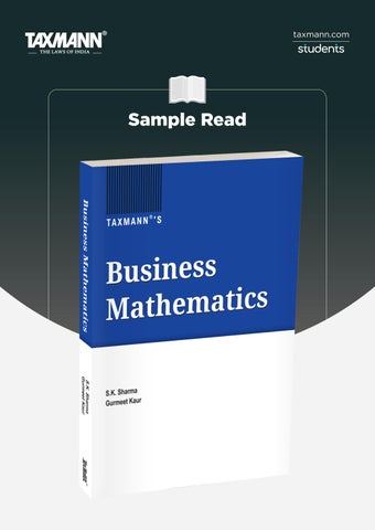
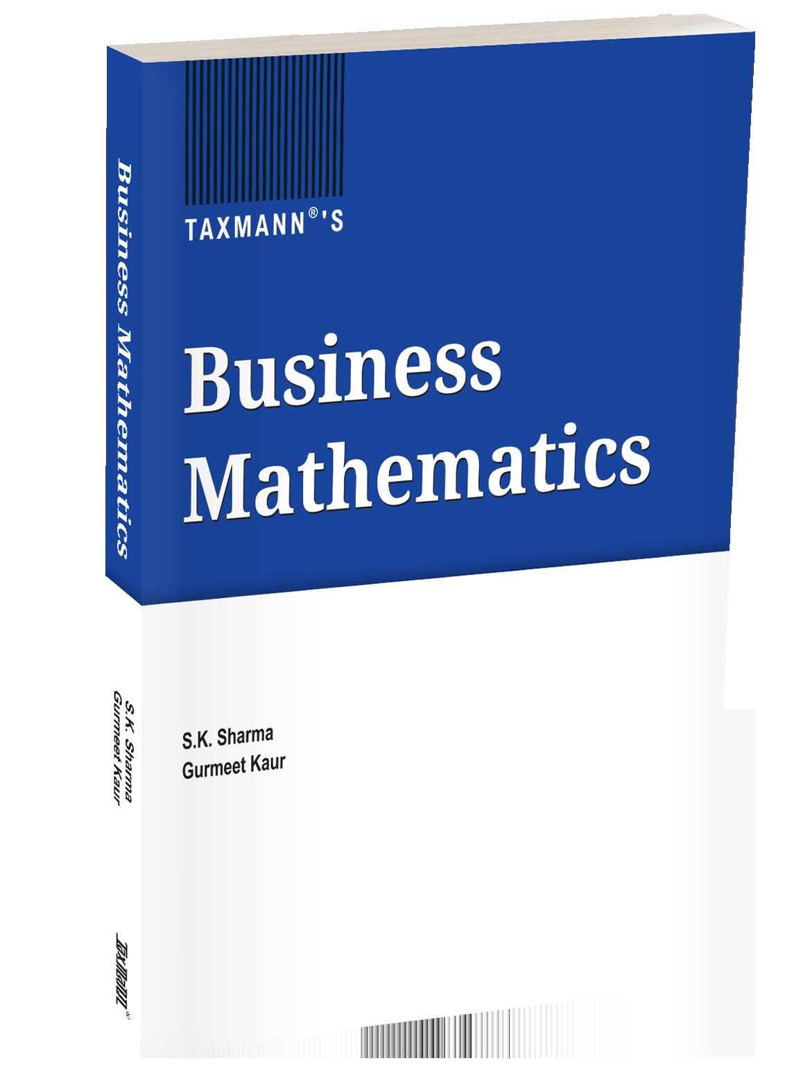
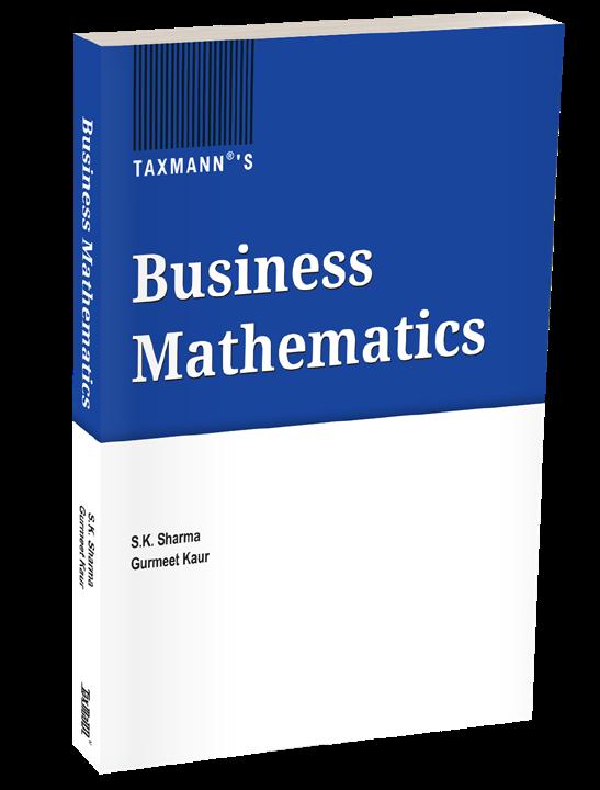
Business Mathematics
AUTHOR : S.K. Sharma, Gurmeet Kaur
PUBLISHER : Taxmann
DATE OF PUBLICATION : July 2026
EDITION : 2026 Edition
ISBN NO : 9789375612544
No. of Pages : 652
BINDING TYPE : Paperback
Rs. 895
DESCRIPTION
Business Mathematics is a comprehensive, application-driven textbook presenting the complete quantitative toolkit a commerce student needs—matrices and determinants, differential and integral calculus, mathematics of finance, and linear programming—through the lens of real business, economic, and financial decision-making.
The book rests on a clear premise: successful business professionals are those who make quick, informed decisions by applying mathematical reasoning to complex situations. Accordingly, no technique arrives as abstract theory. The authors organise the entire treatment around three domains of application:
• Business — Investment decisions, return analysis, sales and profit determination, cost allocation, production capacity utilisation, pricing strategy, commission calculation, product requirement planning, transportation logistics, and optimisation of sales mix and production systems
• Economics — Equilibrium pricing, elasticity of demand and supply, income determination, demand and supply analysis, production and cost functions, revenue assessment, and consumer and producer surplus
• Finance — Effective interest rates, equated payment times, annuities, depreciation schedules, loan amortisation, bond valuation, and sinking funds
What sets the book apart is a structural decision running through almost every chapter: each solved example is mirrored by a same-numbered end-ofchapter exercise posing the identical task with different data—which is why 11 of the 14 chapters carry exactly as many exercises as examples. The student reads the method worked in full, then performs it unaided on parallel data, with an answer supplied for comparison.
Behind that architecture sits a substantial body of worked material: 493 fully solved examples and 486 numbered exercises, every exercise with an answer key and most carrying multiple sub-parts. 294 problems are tagged to actual University of Delhi examination papers from 42 sittings between 1981 and 2026—and 254 of those sit on the solved examples, so the student sees the real exam question worked end to end rather than merely set as practice. Written in deliberately clear language, the book is aimed at beginners and at students who have found mathematics intimidating. Concepts are developed step by step and anchored to Indian, rupee-denominated business contexts—so students learn not merely to compute, but to read what the computation says about the decision at hand. It is structured to align with the B.Com. (Hons.) and B.Com. syllabi under the UGCF–NEP 2020 framework of the University of Delhi, with both syllabi reproduced in full in the front matter, and is equally suited to comparable curricula at other central universities in India and abroad. This book is intended for the following audience:
• B.Com. (Hons.) Students, University of Delhi
• B.Com. Students, University of Delhi
• Students at Other Central Universities in India and Abroad
• Students of Commerce, Economics, Management, and Allied Disciplines
• Beginners and Mathematics-averse Learners
• University of Delhi School of Open Learning (SOL) Students
• Candidates for Professional and Competitive Examinations
• Faculty Seeking a Classroom Text
The Present Publication is July 2026 Edition, authored by S.K. Sharma & Gurmeet Kaur, with the following noteworthy features:
• [Learn It, Then Do It | A Matched-Pair Learning Design] Each solved example is shadowed by a same-numbered exercise posing the same task on fresh data—the book’s defining structural feature, and the reason its example and exercise counts align chapter for chapter
• [Worked in Full | 493 Fully Solved Examples] Numbered continuously within each chapter and weighted toward the application-heavy topics
• [Practice with Answers | 486 Graded End-of-Chapter Exercises] Every one carries an answer key, with multiple sub-parts per question, so the true problem count runs well beyond the numbered total
• [45 Years of the Paper | 294 University of Delhi Past-Paper Questions, Tagged by Year] Spanning 42 sittings from 1981 to 2026, with 254 worked in full as solved examples
• [NEP-aligned Outcomes | Learning Objectives Open All 14 Chapters] Measurable, outcome-based statements using Bloom-style action verbs—Define, Compute, Apply, Analyse, Evaluate, Interpret
• [Revision-ready | KEY FORMULAS Boxes] Closing the six most formula-dense chapters—Input-Output Analysis, Differentiation, Integration, Applications of Integration, Rates of Interest, and Annuities
• [Business Context Throughout | Practical Applications in a Candid and Lucid Fashion] Examples drawn from recognisable Indian business situations
• [Visual Intuition | 62 Numbered Figures Across Eight Chapters] Concentrated where seeing it matters most—Annuities (18 timeline diagrams), Application of Differentiation (16 cost/revenue curves), the spreadsheet chapter (10)—supported by LPP feasible-region graphs and 56 worked simplex tableaux
• [Nothing Skipped | Step-by-Step Solutions] Full working shown at every stage rather than assumed
• [Beyond the Number | Answers That Interpret, Not Just Compute] In the LPP chapters especially, answer keys carry the full economic reading: optimal product mix, maximum revenue, shadow prices, which centre to expand and why, unutilised capacity, and whether the solution is degenerate with reasons
• [Practical-ready | A Dedicated Spreadsheet Practicals Unit (Unit VI)] 43 pages documenting 18 Excel functions argument by argument, plus Solver
• [Value-added Coverage | Content Beyond the Prescribed Minimum] Gauss Elimination and Gauss-Jordan Elimination alongside the syllabus-mandated Matrix Inversion and Cramer’s Rule, and the closed Leontief model as well as the open model the syllabus requires
• [No Extra Books Needed | Self-Contained Appendices] A how-to on reading logarithmic tables, plus seven numbered tables—common logarithmic, antilogarithmic, exponential, FVIF, PVIF, FVIFA and PVIFA