Monitoring rocky reef biodiversity by underwater geo-referenced

Gonzalo Bravo1,2,3,* Juan Pablo Livore1 and Gregorio Bigatti1,2,3,4 1LARBIM, Instituto de Biología de Organismos Marinos (IBIOMAR), CCT CONICET- CENPAT, Puerto Madryn, Argentina 2Universidad Nacional de la Patagonia San Juan Bosco (UNPSJB), Puerto Madryn, Argentina 3Fundación ProyectoSub, Puerto Madryn, Argentina 4Universidad Espíritu Santo (UEES), Ecuador

Received 13 December 2020; Accepted 26 January 2021

Abstract

Digital images are an excellent tool for divers to sample hard-bottom subtidal habitats as bottom time is limited and high-definition images can be collected quickly and accurately. The present paper describes a sampling protocol for benthic rocky reef communities using geo-referenced photoquadrats and tests the method over several rocky reefs of Atlantic Patagonia. This method was tested in two localities, separated by 100 km in a semi-enclosed gulf, covering a total of 5800 m of 11 rocky reefs using track roaming transects. The protocol is non-destructive, relatively low-cost and can adequately assess changes in marine habitats as rocky reefs. The implementation of artificial intelligence analysis using human expert training may reduce analysis time and increase the amount of data collected. The present study recommends this sampling methodology for programs aimed at monitoring changes in biodiversity.

Keywords: scientific diving, benthic survey, global positioning system (GPS), underwater imaging

1. Introduction

Underwater sampling by SCUBA diving is challenging, and cost-effective methods are necessary to efficiently use available bottom time. Videos and still images have been shown to be an excellent tool for divers to sample hard-bottom subtidal habitats. They allow fast sampling which divers can complement with casual or qualitative in situ observations that may help to understand ecological patterns (Underwood et al., 2000).

The benefits and limitations of photoquadrats for subtidal surveys are well described (Preskitt et al., 2004; Sayer and Poonian, 2007; van Rein et al., 2011; Beijbom et al., 2012; Eleftheriou, 2013; Berov et al., 2016; Beisiegel et al., 2017). Among the benefits, less bottom time and non-destructive sampling are the main reasons why photoquadrats are chosen. Despite their limitation for taxonomic resolution, they are an efficient tool for detecting changes in benthic communities (e.g. Parravicini et al., 2009). This type of sampling has been used in several monitoring programmes, such as Census of Marine Life-NAGISA (Rigby et al., 2007), Victorian Subtidal Reef Monitoring Program (Hart et al., 2005), AIMS Long Term Monitoring Program (Thompson et al., 2014); some have included citizen participation (e.g. Reef Life Survey, Edgar and Stuart-Smith, 2014), with taxonomic expertise not a requisite for divers.

With the continuous development of technology, the use of image-based tools for underwater surveys has increased. Digital photography has significantly improved image resolution, sensor sensitivity, image compression, battery life, apparatus size and cost. Therefore, photoquadrats should display improved quality, and combined with extra instruments (e.g. GPS, depth loggers) and basic computer skills, post-analysis should become easier and faster. Recent advances in machine learning for automated or semi-automated analysis of photoquadrats have shown promising results (Beijbom et al., 2015; González-Rivero et al., 2016; Gormley et al., 2018; Williams et al., 2019). The adequate use of this method of image analysis can aid in closing the gap between the rapid acquisition of numerous images and their required processing time.

Underwater sampling protocols are often adapted or modified after field-testing under variable conditions as visibility, currents, depth, type of

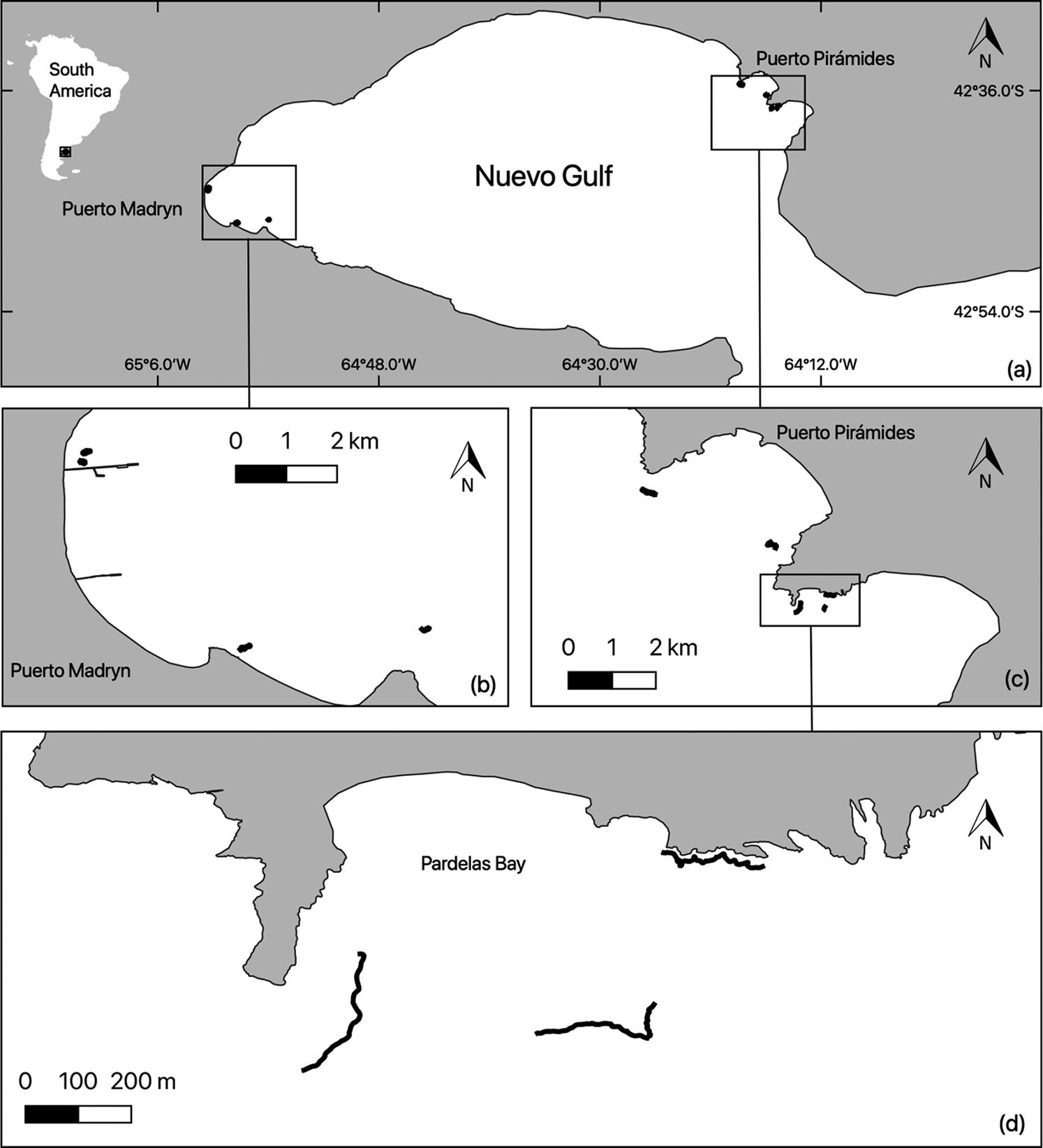
Fig 1: (a) Study site with black dots representing rocky reefs sampled; (b) southwest regions; (c) northeast regions; and (d) close-up of Pardelas Bay. Black lines represent the tracked transects on three reefs Fig 2: Diagram of diver with the sampling equipment: GPS buoy on the surface; PARALENZ (www.paralenz.com) video camera on the diver mask; underwater camera with flashes and stainless-steel structure frame. H = horizontal surfaces; V = vertical surfaces; O = overhang surfaces; and C = cavefloor surfaces. Original reef drawing by Gaston Trobbiani

habitat, etc. Small upgrades are not often shared in scientific articles, although some online platforms (e.g. protocols.io, ocean best practices) include this information and keep it up to date.

In Nuevo Gulf, Atlantic Patagonia (Fig 1), several rocky reefs provide an excellent scenario to test sampling methodologies. The rocky reef extensions range from 100 m to more than 1500 m, and shapes are normally lineal with an edge that gives place to small caves (see Fig 2). The present paper describes a sampling protocol for benthic rocky reef communities using geo-referenced photoquadrats and testing the method over several rocky reefs of Atlantic Patagonia.

2. Materials and methods 2.1 Equipment set-up

For the photoquadrats, a Canon 100D (SL1) camera placed in an Ikelite housing up to 60 m depth rating was used. This camera is one of the smaller and cheaper options for DSLT underwater photography, and a full-change battery can take more than 400 photos in water temperature between 12 °C–18 °C. The camera used had an 18 mm–55 mm Canon lens, and all images were taken with a focal length of 18 mm, auto focus, ISO 400 and exposure 1/200 s at f/11. As most underwater professional photographers recommend strobes for still photography, two Ikelite DS-161 strobes were used. These flashes provide more than 300 shoots (in the temperature range 12 °C–18 °C), which is a much greater amount than that provided by continuous dive lights. The through-the-lens (TTL) function was used in order to have optimal lighting in each photo, and the directions of strobes were crucial to avoid backscatter in low visibility conditions (Fig 3).

The system was mounted on a rigid stainless steel structure with a 50 cm distance between the lens and the sea floor, giving a 0.0625 m2 quadrat (0.25 m × 0.25 m) in the middle of the photo. A stainless steel structure (not PVC as in Bravo et al., 2015) of 6 mm diameter was used in order to increase the stability and resistance of the tetrapod. The latter is important when taking photos in rough conditions such as strong currents or shore breaks which can cause the camera frame to suffer substantial collisions. The stainless steel structure was painted in order to avoid flash reflection. The camera and strobes were attached to the stainless steel tetrapod by a Velcro system that allowed removal of the camera from the structure whilst diving if a close-up photo is needed. The frame, camera and flashes weighed a total of 8.8 kg, which needed to be taken into consideration for the diving weight calculations.

A dive computer (Oceanic Geo2) was mounted on one side of the quadrat to record depth (± 0.3 m) and temperature (±1 °C) of each photo. This information was used for descriptive and comparative purposes; for precise use of this type of data, computers should be accurately calibrated (see Azzopardi and Sayer, 2012). Divers carried a PARALENZ video camera (https://www.paralenz.com) on the

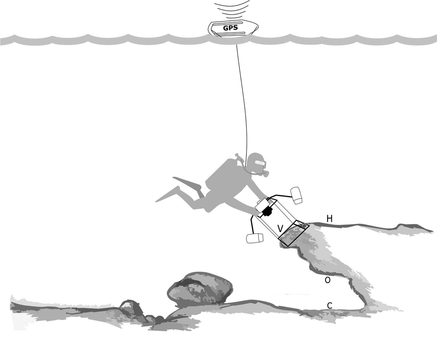
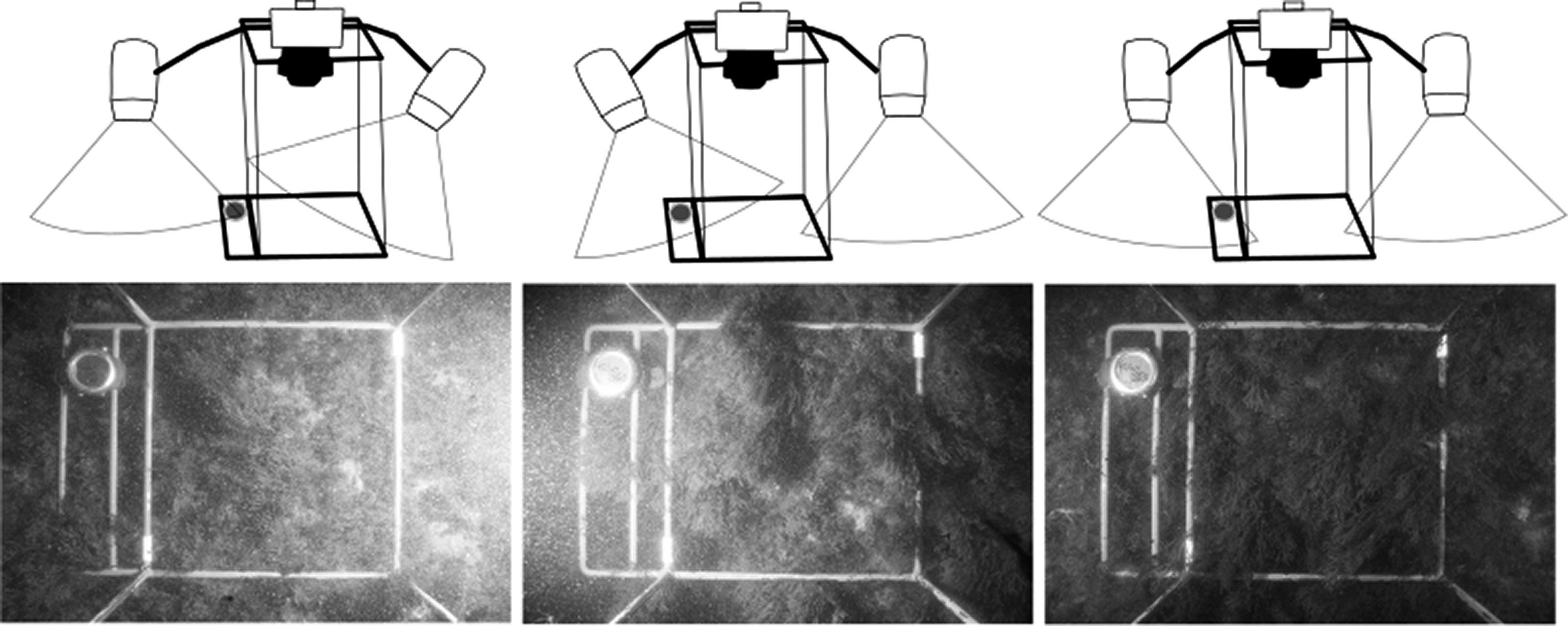
Fig 3: Flash direction and its effect on backscattering under low visibility conditions. The diving computer can be seen in the top left of the photos

mask filming the transect, and recording depth and temperature. The information from these videos was used to characterise the rocky reefs (results not presented in this paper).

A zodiac boat followed the divers’ path with the buoy on the surface as reference. When dives were performed without zodiac assistance, the reef was not further than 300 m from the coast line; a diver supervisor followed the buoy and assisted with the entrance and exit at sites that were explored before each dive.

3. Sampling

Photoquadrats separated by at least 1.5 m were taken randomly along tracked roaming transects on the rocky reef. The presence of cavities with heights of 1.5 m–3 m below the rocky reef ledges provided enough space to sample four different surface orientations (horizontal, vertical, overhang and cave floor; Fig 2); when the cavities were smaller, only horizontal and vertical surfaces were sampled. Horizontal and vertical surface orientations were sampled in all reefs. In order to compare rocky reefs from two regions of Nuevo Gulf, six rocky reefs in the southwest and five reefs in the northeast were sampled during the same year. Reefs were separated by more than 100 m within each region.

3.1. Georeferencing photoquadrats The geolocation procedure used for transects was: 1) GPS and camera time were synchronised. This was done by aligning the camera clock with the

GPS clock before each dive. 2) The GPS was set on track mode recording one waypoint every 3 seconds. 3) The portable GPS (e.g. Garmin etrex 10) was placed in a dry bag on top of a rescue can buoy connected to the diver by a monofilament line using a diving reel (Fig 2). The use of two GPS devices on the buoy was ideal to reduce the risk of losing data caused by low battery or other drawbacks of the GPS. 4) Divers maintained the monofilament line as tightly as possible in order to avoid angles between the buoy and the diver. This could produce a vertical force over the diver, and the reel with the line needed a safety fast release. 5) At the end of the survey, divers saved the track file on the GPS. 6) Photos were georeferenced using the function

‘Auto-tag photos’ in Adobe Lightroom Classic version: 9.1. This software allows uploading of .gpx files and synchronises photos using time.

Other options for performing this task are:

GPS-Photo Link software, the open-source code

‘benthic photo survey’ (Kibele, 2016) or a customised R code (e.g. https://github.com/gonzalobravoargentina/photoquadrats). 7) GPS position was stored on the metadata of each photo, and this information could be processed in a GIS software.

3.2. Image analysis Images were prepared for analysis using photo processing software (Adobe Lightroom Classic version: 9.1). Lightroom presents many functionalities which improve the organisation and processing of photos, such as the ‘Auto Sync’ tool which allows changes to be applied to a set of photos (e.g. cropped area of interest, lens corrections, addition of metadata). All images passed through the same workflow in the Lightroom program:

(1) geo-referencing with the gpx file using ‘Autotag photos’; (2) including depth, site and surface orientation data on photo´s metadata; (3) white balance selecting a white tape on the frame; (4) cropping the area of interest (0.25 m × 0.25 m); and (5) automatic lens distortion correcting using the lens profile. Blurry or out-of-focus images were discarded and those that were too dark or bright were corrected.

In order to follow the same guidelines in the metadata information, depth was included on the elevation field, surface orientation was included in the caption field, and site was included on the sublocation field in the Lightroom program. The process of including depth on the metadata information can be time demanding as it must be done individually for each photo in Lightroom. An alternative would be to use an R code to merge GPS, depth and temperature data to each photo and obtain a .csv file (e.g. https://github.com/gonzalobravoargentina/photoquadrats).

The photoquadrat analyses were performed in CoralNet (https://coralnet.ucsd.edu). This open source and free software can be used from any computer via an internet server and allows several users to work on the same source. The metadata for all photos was uploaded using a .csv file that was created by reading photo metadata by R code. While some studies suggested changing the photo name in order to have all metadata information included in the file name, it was noted that leaving the original name of the photo or an ID number allows faster filtering when using CoralNet and Lightroom. Percentage cover of algae and sessile invertebrates was calculated using a 100-point grid overlaid on each photo. Grid points lacking substrate were removed and percentage cover of each taxa was recalculated without these. All slow mobile fauna per image were counted to calculate density of each species.

At the end of the process three matrices were obtained: 1) percentage cover; 2) density; and 3) presence-absence combining species from cover and density data. Some species that are difficult to identify by photo were grouped in a category or taxonomic group using the classification proposed

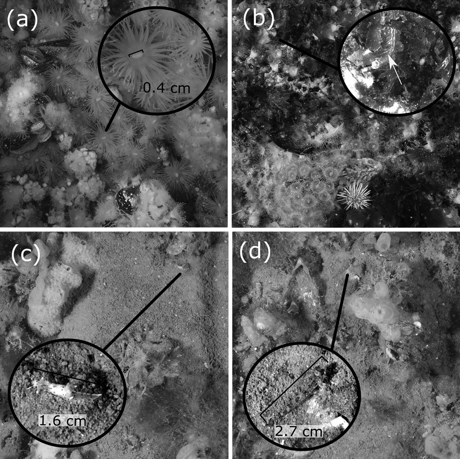
Fig 4: Cropped photoquadrats (0.25 m × 0.25 m) examples. Close-ups to show image definition of: (a) anemone; (b) ribs on laminated algae; (c) nudibranch; and (d) small benthic fish

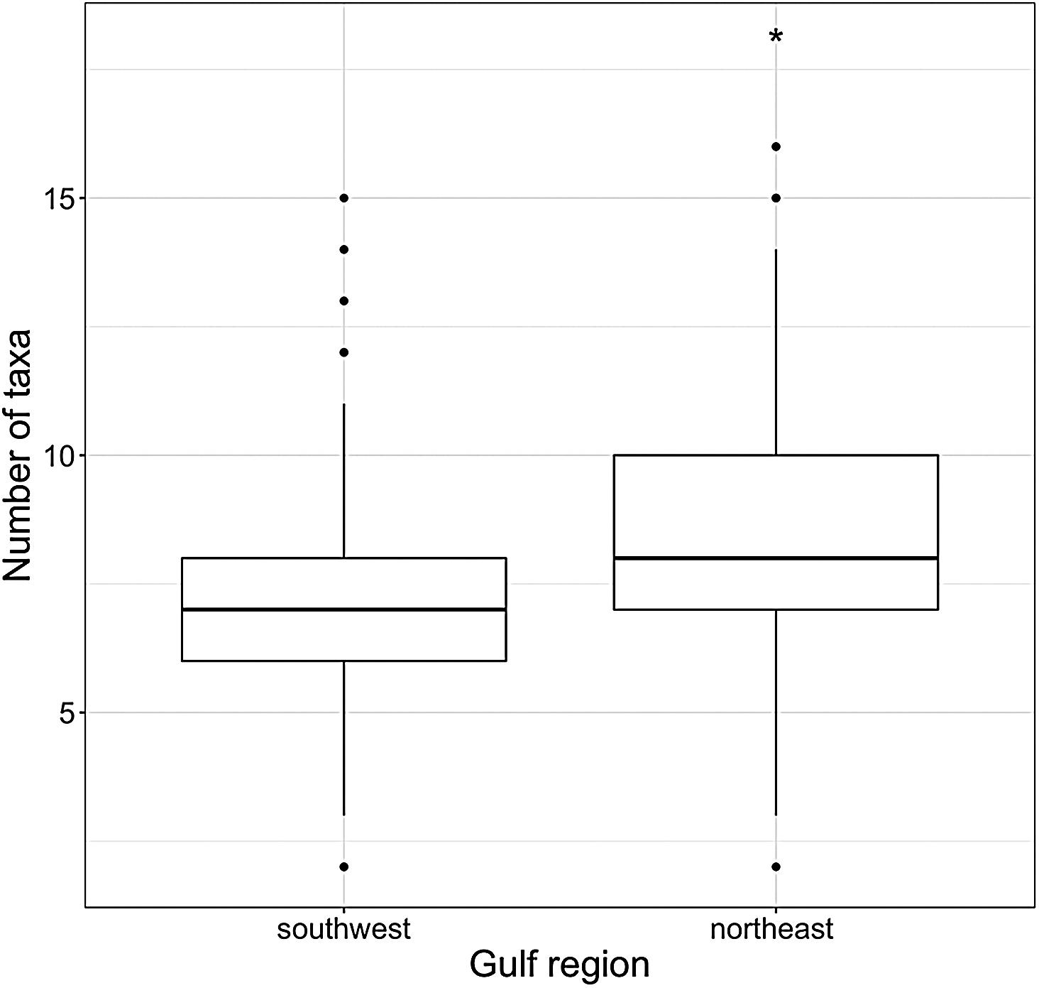
Fig 5: Boxplot of taxa richness among southwest (n = 424 photoquadrats) and northeast (n = 470 photoquadrats) region of Nuevo Gulf. The * indicates p < 0.001, obtained by randomisation test using the R package ‘rich’ (Rossi, 2011) with the presence-absence matrix of horizontal and vertical surfaces as input

by the Collaborative and Automated Tools for Analysis of Marine Imagery (CATAMI, Althaus et al., 2015) to standardise the analysis. As CoralNet provides machine learning, all photos analysed manually served to train the robot of the source.

4. Results and discussion

The underwater survey protocol using georeferenced photoquadrats to estimate percentage cover and density of epibenthic communities was tested, with good results obtained under various conditions of visibility, water currents and low water temperature at two zones (northeast and southwest) of Nuevo Gulf, Patagonia. Of note is that all bottom time was used for displacement and taking photos, which allowed the exploration of larger areas; this is important when studying habitats with high spatial heterogeneity (Beisiegel et al., 2020). A total of 20 transects were performed, covering 5800 m of rocky reefs during seven diving days. On average, transect length was 305.65 m (SD:149 range: 101–629), which took 25 minutes (SD:11.11, range:1147) at a depth range of 2 m -15 m and an average speed of 0.77 km/hr with more than 123 photos per transect. The extension of the survey could be increased using underwater scooters (see Bryant et al., 2017). However, this involves a higher cost, more logistics and greater difficulty upon water entry on shore dives.

The use of flashes for photoquadrats resulted in high-quality images that enabled the detection of small species with good definition (Fig 4a, c, d; for more examples, see https://coralnet.ucsd.edu/ source/1933/), and assisted in taxonomic identification. In some cases, the observation of morphological features such as ribs on laminated algae was useful for genus or family distinction (Fig 4b). Species that were difficult to identify by photo (e.g. Porifera and colonial tunicates) were pooled into functional groups in accordance with the CATAMI classification scheme which has well described and updated documentation. As the images are stored on the CoralNet server and the annotations are searchable, it is possible to review previous annotations. The latter feature also helps to train new users with the taxa identification. Photoquadrats (n = 894) detected 76 taxa in total in the Nuevo Gulf region. The northeast region presented a higher richness (65 versus 53) and a greater number of species per quadrats than the southwest sites (Fig 5).

Small (<5 cm) cryptic fish species such as Helcogrammoides cunninghami (Fig 4c) were distinguished on images, and density estimations using photoquadrats should be compared with visual quadrats under the same conditions in order to test if the method presented in the present study is adequate for cryptic fish estimations. This protocol was designed for estimation of cover and abundance of benthic sessile or slow moving species. However, incorporating visual census for estimation of fish abundance and diversity, similar to Reef Life Survey (2017), will improve the present study’s data. The videos recorded by the Paralenz camera carried by divers were unstable and unsuitable for fish counts, and were only used for describing the habitat.

The most common method for fine-scale sampling on rocky bottoms is quadrats along transects with a variation in quadrat size (1 m2, 0.25 m2 and 0.0625 m2). The choice of the sampling unit should consider the size of the sampled organism and the aggregation among them (Underwood and Chapman, 2013). However, in subtidal habitats water visibility must also be considered when using photoquadrats. In most parts of the Atlantic Patagonian coasts, visibility ranges from 0.5 m to 10 m (with an average of 4 m), and in order to obtain a 0.50 m × 0.50 m photoquadrat the camera must be positioned at least 0.60 m from the bottom. Under low visibility this distance results in poor-quality photos which are unsuitable for analysis. The present study used 0.25 m × 0.25 m quadrats, as the resulting photoquadrats were suitable under various visibility conditions. Concurrently, a large number of small-sized quadrats rather than fewer larger-sized quadrats represent the spatial variability with better accuracy (Bohnsack, 1979; Andrew and Mapstone, 1987; Sayer and Poonian, 2007).

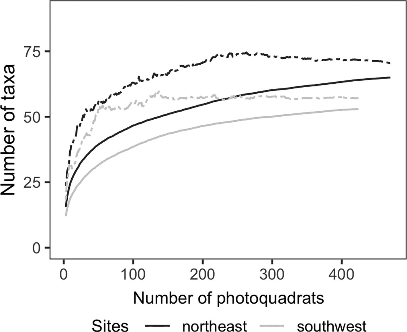
Fig 6: Taxa accumulation curve and expected number of taxa (Chao2 = dashed lines) for rocky reefs assemblages on northeast and southwest sites in Nuevo Gulf. Calculated with the ‘poolaccum’ function of the ‘Vegan’ R package (Oksanen et al., 2019)

The use of track roaming transects provided numerous benefits, such as: 1) time is not spent having to deploy tape measures; 2) each photoquadrat is geo-referenced for better accuracy, which provides coordinates to return to a specific area of interest; 3) the path is not required to be straight; 4) parts of the reef that are not suitable for sampling can be avoided; and 5) GPS position assists in labelling photos by transect, site and location. Although portable GPS devices have been available since the early 1990s, existing literature that used geo-referencing techniques on subtidal photoquadrats is scarce. There are some examples that used similar techniques for fish census (Lynch et al., 2015; Irigoyen et al., 2018) and benthic surveys (Roelfsema and Phinn, 2009; Niedzwiedz and Schories, 2011; Sanamyan et al., 2015). However, most likely owing to the added complexities on diving logistics, the use of GPS devices on surface buoys is not a common practice. Other options with the same principle and floating antennas include the GPS diving computer (Kuch et al., 2012) or a GPS inside a housing (Niedzwiedz and Schories, 2014). However, the use of cables presents additional problems (Niedzwiedz and Schories, 2014) and cables often do not resist the same strain as ropes.

In the present study, the use of a robust floating device (rescue can buoy) presented good hydrodynamics and enabled tensing of the cord to provide less difference between the position of the diver and the GPS. Recently developed technologies for underwater geolocation offer high precision without the use of cables or ropes, giving greater freedom to divers (https://uwis.fi/en). However, the costs of these technologies are high which limits the ubiquity of their use globally.

Species accumulation curves are often used for determining the sampling effort (i.e. minimum number of photoquadrats) to obtain reliable estimations of richness (Ugland et al., 2003). Species accumulation curves performed for southwest and northeast sites in the Nuevo Gulf showed that with 200 photos the horizontal asymptote is nearly reached, capturing 87 % and 85 % of the total species richness in each gulf area, respectively (Fig 6). This shows that the actual number of photoquadrats per transect (~124) should be increased in order to achieve a better estimation of richness. However, increasing this number is challenging owing to the time required for analysis. Artificial intelligence could help to reduce this processing time, enabling a greater number of photos and better estimations of richness. CoralNet software provides semi- and fully-automated annotations after a large set of photos are analysed by experts. The Alleviate operational mode (semi-automated) decides when to make an automated annotation using a classification score. Beijbom et al. (2015) showed that 50 % of the annotations performed by the robot had no effect on the quality of percentage cover of estimates of 20 categories. Using this mode for processing photoquadrats can increase the total number of photoquadrats analysed.

The non-destructive and relatively low-cost protocol of our study can adequately assess changes in marine habitats as rocky reefs (as was shown in the same area of the present paper; see Bravo et al., 2020) which provide important ecosystem services. Essential Ocean Variables (EOVs; Miloslavich et al., 2018) such as macroalgal cover, benthic invertebrate abundance and benthic invertebrate diversity can be estimated with this methodology. This is useful for broad scale monitoring programmes such as MBON (Duffy et al., 2013). The present method relies on high-quality, underwater images taken under a standardised method, which reduces the variation in photo resolution, angle of view, distance to the sea floor, and compensation of light attenuation, and will assist with the implementation of artificial intelligence analysis that may be affected by these variations.

Acknowledgement

The present authors are grateful to the divers and technicians who participated in the field work: Ricardo Vera, Néstor Ortiz, Facundo Irigoyen, Fabián Quiroga, Julio Rua, Nicolás Battini, Claudio Nicolini, Yann Herrera Fuchs, Axel Schmid, Gastón Trobbiani and Alejo Irigoyen. Special thanks are

given to Punta Ballena (https://www.puntaballena. com.ar) for logistical assistance in Puerto Pirámides. Field studies in Natural Protected Areas were done under permit (Nº 014- MTyAP-19). The present work was funded by Patagonia Inc. (grant award TF2002-089196), Rapid Ocean Conservation grant (Waitt Foundation-https://www.waittfoundation. org) and PICT-2018-0969 (ANPCyT- ARGENTINA). This is publication number 147 of LARBIM.

References

Althaus F, Hill N, Ferrari R, Edwards L, Przeslawski R,

Schönberg CHL, Stuart-Smith R, Barrett N, Edgar G,

Colquhoun J, Tran M, Jordan A, Rees T and Gowlett-

Holmes K. (2015). A standardised vocabulary for identifying benthic biota and substrata from underwater imagery:

The CATAMI classification scheme. PLOS ONE 10: 1–18. Andrew NL and Mapstone BD. (1987). Sampling and the description of spatial patterns in marine ecology. Oceanography and Marine Biology 25: 39–90. Azzopardi E and Sayer M. (2012). Estimation of depth and temperature in 47 models of diving decompression computer. Underwater Technology 31: 3–12. Beijbom O, Edmunds PJ, Kline DI, Mitchell BG and Kriegman D. (2012). Automated annotation of coral reef survey images. In: Proceedings of 2012 IEEE Conference on Computer Vision and Pattern Recognition, 16–21 June,

Providence, USA, 1170–1177. Beijbom O, Edmunds PJ, Roelfsema C, Smith J, Kline DI,

Neal BP, Dunlap MJ, Moriarty V, Fan TY, Tan CJ, Chan S,

Treibitz T, Gamst A, Mitchell BG and Kriegman D. (2015). Towards automated annotation of benthic survey images: Variability of human experts and operational modes of automation. PLOS ONE 10: 1–22. Beisiegel K, Darr A, Gogina M and Zettler ML. (2017). Benefits and shortcomings of non-destructive benthic imagery for monitoring hard-bottom habitats. Marine Pollution Bulletin 121: 5–15. Beisiegel K, Darr A, Zettler M, Friedland R, Gräwe U and

Gogina M. (2020). Spatial variability in subtidal hard substrate assemblages across horizontal and vertical gradients: a multi-scale approach by seafloor imaging. Marine

Ecology Progress Series 633: 23–36. Berov D, Hiebaum G, Vasilev V and Karamfilov V. (2016).

An optimised method for scuba digital photography surveys of infralittoral benthic habitats: A case study from the SW Black Sea Cystoseira-dominated macroalgal communities. Underwater Technology 34: 11–20. Bohnsack JA. (1979). Photographic quantitative sampling of hard-bottom benthic communities. Bulletin of Marine

Science 29: 242–252. Bravo G, Márquez F, Marzinelli EM, Mendez MM and Bigatti

G. (2015). Effect of recreational diving on Patagonian rocky reefs. Marine Environmental Research 104: 31–36. Bravo G, Livore JP and Bigatti G. (2020). The importance of surface orientation in biodiversity monitoring protocols:

The case of Patagonian rocky reefs. Frontiers in Marine Science 7: 1–12. Bryant DEP, Rodriguez-Ramirez A, Phinn S, González-

Rivero M, Brown KT, Neal BP, Hoegh-Guldberg O and

Dove S. (2017). Comparison of two photographic methodologies for collecting and analyzing the condition of coral reef ecosystems. Ecosphere 8: 1–17. Duffy JE, Amaral-Zettler LA, Fautin DG, Paulay G, Rynearson TA, Sosik HM and Stachowicz JJ. (2013). Envisioning a marine biodiversity observation network. BioScience 63: 350–361. Edgar GJ and Stuart-Smith RD. (2014). Systematic global assessment of reef fish communities by the Reef Life

Survey program. Scientific Data 1: 1–8. Eleftheriou A (ed.). (2013). Methods for the study of marine benthos. 4th edition. Chichester: John Wiley & Sons, pp. 496 González-Rivero M, Beijbom O, Rodriguez-Ramirez A,

Holtrop T, González-Marrero Y, Ganase A, Roelfsema C,

Phinn S and Hoegh-Guldberg O. (2016). Scaling up ecological measurements of coral reefs using semi-automated field image collection and analysis. Remote Sensing 8: 30. Gormley K, McLellan F, McCabe C, Hinton C, Ferris J, Kline

DI and Scott BE. (2018). Automated image analysis of offshore infrastructure marine biofouling. Journal of

Marine Science and Engineering 6: 1–20. Hart SP, Edmunds M, Elias J and Ingwersen C. (2005). Victorian subtidal reef monitoring program: The reef biota on the western Victorian coast. Parks Victoria Technical

Series. Number 72. Vol 2. Melbourne: Parks Victoria.

Available at: https://www.yumpu.com/en/document/ view/31797052/victorian-subtidal-reef-monitoring-program-parks-victoria, last accessed <7 February 2021>. Irigoyen AJ, Rojo I, Calò A, Trobbiani G, Sánchez-Carnero

N and García-Charton JA. (2018). The ‘Tracked Roaming Transect’ and distance sampling methods increase the efficiency of underwater visual censuses. PLOS ONE 13: 1–15. Kibele J. (2016). Benthic photo survey: Software for geotagging, depth-tagging, and classifying photos from survey data and producing shapefiles for habitat mapping in

GIS. Journal of Open Research Software 4: 1–5. Kuch B, Buttazzo G, Azzopardi E, Sayer M and Sieber A. (2012). GPS diving computer for underwater tracking and mapping. Underwater Technology 30: 189–194. Lynch T, Green M and Davies C. (2015). Diver towed GPS to estimate densities of a critically endangered fish. Biological Conservation 19: 700–706. Niedzwiedz G and Schories D. (2011). GPS supported monitoring by scientific divers within a Chilean-German

Antarctic project. In: Paschen M and A Soldo (eds.).

Contributions on the theory of fishing gears and related marine systems 7: 13–24. Niedzwiedz G and Schories D. (2014). Advances using divertowed GPS receivers. In: Ya-Hui H (ed.). Global positioning systems: Signal structure, applications and sources of error and biases. New York: Nova Science Publishers, 155–186. Oksanen J, Blanchet FG, Friendly M, Kindt R, Legendre P,

MsGlinn D, Minchin PR, O’Hara RB, Simpson GL, Solymos P, Stevens HHM, Szoecs E and Wagner H. (2019).

Vegan: Community Ecology Package. R package version 2.5-5. Available at: http://packages.renjin.org/package/ org.renjin.cran/vegan, last accessed <7 February 2021>. Parravicini V, Morri C, Ciribilli G, Montefalcone M, Albertelli G and Bianchi CN. (2009). Size matters more than method: Visual quadrats vs photography in measuring human impact on Mediterranean rocky reef communities. Estuarine, Coastal and Shelf Science 81: 359–367. Preskitt LB, Vroom PS and Smith CM. (2004). A rapid ecological assessment (REA) quantitative survey method for

Benthic algae using photoquadrats with scuba. Pacific Science 58: 201–209.

Rigby PR, Iken K and Shirayama Y (eds.). (2007). Sampling biodiversity in coastal communities: NaGISA protocols for seagrass and macroalgal habitats. Kyoto: Kyoto University

Press, pp. 160 Roelfsema CM and Phinn SR. (2009). A manual for conducting georeferenced photo transects surveys to assess the benthos of coral reef and seagrass habitats. Version 3.0. Brisbane: University of Queensland. Available at: https://epic.awi.de/id/eprint/31165/1/GPS_Photo_

Transects_for_Benthic_Cover_Manual.pdf, last accessed <7 February 2021>. Rossi JP. (2011). rich: An R package to analyse species richness. Diversity 3: 112–120. Sanamyan NP, Sanamyan KE and Schories D. (2015). Shallow water Actiniaria and Corallimorpharia (Cnidaria:

Anthozoa) from King George Island, Antarctica. Invertebrate Zoology 12: 1–51. Sayer MDJ and Poonian C. (2007). The influences of census technique on estimating indices of macrofaunal population density in the temperate rocky subtidal zone. Underwater Technology 27: 119–139. Thompson AA, Lønborg C, Costello P, Davidson J, Logan

M, Furnas M, Gunn K, Liddy M, Skuza M, Uthicke S,

Wright M, Zagorskis I and Schaffelke B. (2014). Marine Monitoring Program. Annual Report of AIMS Activities 2013–2014. Inshore water quality and coral reef monitoring. Report for the Great Barrier Reef Marine Park

Authority. Townsville: Australian Institute of Marine Science. Available at: https://elibrary.gbrmpa.gov.au/ jspui/handle/11017/2975, last accessed <7 February 2021>. Ugland KI, Gray JS and Ellingsen KE. (2003). The species–accumulation curve and estimation of species richness.

Journal of Animal Ecology 72: 888–897. Underwood AJ, Chapman MG and Connell SD. (2000).

Observations in ecology: you can’t make progress on processes without understanding the patterns. Journal of

Experimental Marine Biology and Ecology 250: 97–115. van Rein H, Schoeman DS, Brown CJ, Quinn R and Breen J. (2011). Development of benthic monitoring methods using photoquadrats and scuba on heterogeneous hardsubstrata: A boulder-slope community case study. Aquatic

Conservation: Marine and Freshwater Ecosystems 21: 676–689. Williams ID, Couch CS, Beijbom O, Oliver TA, Vargas-angel

B, Schumacher BD and Brainard RE. (2019). Leveraging automated image analysis tools to transform our capacity to assess status and trends of coral reefs. Frontiers in

Marine Science 6: 1–14.