Industry Threshold

How Can Microfracturing Improve Reservoir Management

Mayank Malik - Formation Testing Expert at Chevron, Houston, Texas

Introduction Hydraulic fracturing has changed the landscape of hydrocarbon production and reservoir dynamics, especially in unconventional reservoirs, and has also proved to be very successful in conventional reservoirs, but “getting it right” can still be very challenging for profitable production. One important factor for success is having accurate and sufficient knowledge of the stress profile across the reservoir. Historically, Hubbert and Willis (1957) discussed the relation between overburden and horizontal stress and showed experimental results indicating that hydraulic fractures will propagate perpendicular to the minimum confining stress. Asset teams are interested in how the in-situ stress field affects the rock’s response to engineering activity, such as drilling and hydraulically fracturing wells. There are several techniques for determining the in-situ state of stress, such as wireline logs and various injection tests.

Injectivity tests use the pressure response during the initiation, propagation, and closure of a hydraulic fracture to directly determine the state of stress. Compared with leakoff tests (LOT) or diagnostic fracture injection tests (DFIT), microfracturing tests are focused and faster (Nguyen and Cramer, 2013; Malik et al., 2014). Microfracturing targets short intervals of about one meter, rather than several meters (Desroches et al., 1995). Therefore, this technology enables testing of a specific reservoir zone or lithology. The injected volumes have been reduced from barrels to liters. Consequently, the shut-in times between injections are shorter. As a result, many intervals may be tested quickly.

Microfracturing Technique Wireline formation testers can be used to determine the minimum in-situ stress within a wellbore interval. A microfracture is created by increasing fluid pressure between two inflated packers or by inflating a single packer to directly breakdown the formation (Fig. 1). The minimum stress is determined by allowing controlled volumes of fluid to leakoff into the microfracture. The technique may be repeated multiple times (injection/falloff cycles) during a single trip.

During each cycle, a certain volume of fluid is injected into the packer interval, the planned volume should be derived using the desired fracture half-length, Young’s modulus of the rock being tested, the net pressure encountered after fracture initiation, and an estimated fracture height. After that, the operators stop the injection, record instantaneous shut-in pressure (ISIP), and monitor the formation leakoff for signs of closure by plotting pressure versus G-function time (Nolte, 1979) and pressure versus the square-root of time (SQRT). Under normal leakoff conditions, the pressure decline is a linear function with respect to the G-function and can be used to interpret closure pressure and time. The closure pressure is the pressure at which the fracture closed completely after shut-in and it is considered an accurate measure of the minimum stress normal to the fracture surface. The basic procedure of the microfracture test is illustrated in (Fig. 2).

Fig. 2 - A hypothetical microfracture response showing fracture initiation, propagation, and closure for two cycles.

Returning to hydrostatic pressure between cycles gives a better reopening pressure measurement on the subsequent cycle. These injection/falloff cycles can be repeated multiple times in order to reopen, further propagate, and close the fracture. Cycles are repeated until an agreement is reached that a dependable and repeatable fracture closure (i.e., minimum in-situ stress) has been recorded.

Fracture initiation pressure must overcome the hoop stress to initiate a fracture. The dominance of hoop stress could result in a false high minimum horizontal stress measurement (Fig. 3); therefore, ensure that total injected volume is high enough to propagate the fracture at least four wellbore radii away; otherwise, the closure pressure derived from microfracturing is not representative of the formation.

Microfracturing vs. DFIT Microfracturing is typically performed in vertical, openhole pilot wells whereas DFITs are usually performed in the first stage of the cased hole lateral. Table 1 compares these two injectivity testing techniques. Compared to DFITs, microfracture tests are fast and focused. A DFIT is usually pumped with a frac pump

which cannot pump slowly. This commonly leads to unconfined height growth, a large fracture diameter and “penny” fracture geometry.

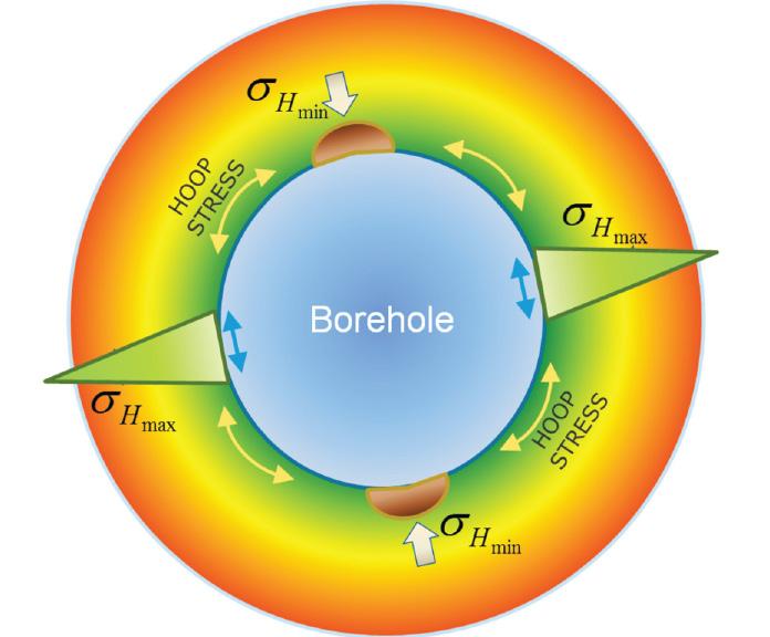
Fig. 3 - Hoop stress concentrates around the near-wellbore region during drilling operations.

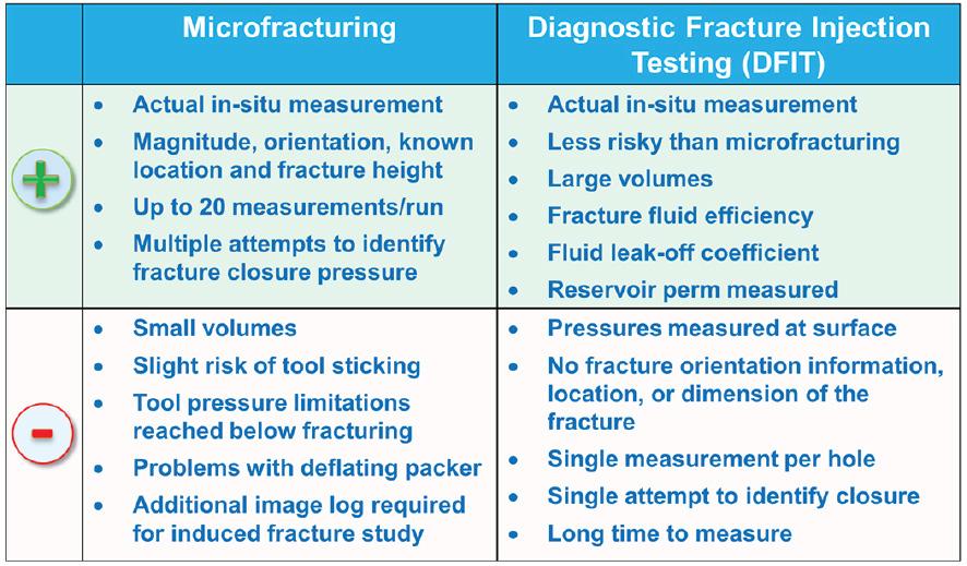
Fig. 4 - Pressure vs. time plot of one of the microfracture tests performed in the Avalon Shale (Delaware Basin). Figure 5 displays the SQRT plot for the first falloff cycle. Closure pressure is measured at the time when the pressure during shut-in deviates from a linear trend on the square-root of shutin time. Since the fracture is induced over a relatively short (3.3- ft) straddled interval, the closure time is only 7.9 min for the first cycle and the closure pressure is 5,575 psi.

Table. 1 - Comparison of Microfracturing vs. DFIT. By contrast, a microfracturing job is pumped so slowly that the height growth is contained. This extremely slow rate translates to a very small fracture diameter, so the ratio of (fracture length) / (volume pumped) is orders of magnitude higher for microfracture than DFIT. Formation tester microfractures incorporate a downhole hydraulic pump, at least one downhole quartz pressure gauge, and provides real-time control through the wireline cable. Thus, microfracturing is similar to using a “downhole rock mechanics lab” for economically obtaining vertically distributed stress measurements prior to casing and completing the well. By combining microfracturing in an open hole with DFITs in a cased hole, the understanding of the stress state, its variation, and its influence on hydraulic fracturing can be substantially improved, thereby enhancing the fracturing test results (Naidu et al., 2015).

Case Study 1: Delaware Basin, USA Seven lithofacies across the Avalon shale and Bone Spring sands were targeted for obtaining independent direct measurements of closure stresses with a microfracturing tool.

Figure 4 shows a pressure vs. time plot for a microfracture test. Two injection and falloff cycles were performed in succession at the same depth to validate consistency and repeatability. The total volume of drilling mud injected in the fracture is 2.7 liters. In the first falloff, an ISIP of 5,695 psi was observed, whereas when the test was repeated, an ISIP of 5,675 psi was observed. ISIP is not used to determine the minimum stress but still can be used as an upper boundary for closure pressure and for comparison with the square-root of time, G-Function, and other results. Fig. 5 – Square root of time vs. pressure plot from the first falloff cycle of the microfracture test.

Case Study 2: North Sea, UK Water injection is used in a field located in the outer Moray Firth to maintain reservoir pressure above the bubblepoint. In the target reservoir sections, the injection pressure is constrained to 14.9 lbm/gal to minimize any risk of seal breach. However, there was a general lack of information on the rock stresses in the overlying caprock intervals. The injection pressures were constrained on values derived from sonic logs. There was a general concern that the injector wells might be over constrained.

Wireline stress measurements using microfracturing were used to determine a more accurate minimum horizontal stress in the overlying formations (Fig. 6), allowing a substantial increase in the water injection rate and a 1,000 to 2,000 BOPD increase in oil production.

Fig. 6 - Pressure vs. time plot for the microfracture test in the caprock.

How “Non-Unique” is Reservoir Simulation Really?

Dwayne Purvis, P.E. - Consultant, Reservoir Engineering and Management

When someone asserts that reservoir simulation generally isn’t worth the time and effort because the results are “non-unique”, they show to me how shallow their experience and insight really are. First and foremost it tells me that they have never tried to come up with one of those (supposedly) many solutions. It can be hard to find even a single history match! Since the person making the complaint has little or no experience with modeling, then it is easy to see why they do not comprehend good model-building or the value it generates. In a century of our discipline, we have only identified six methods for the estimation of reserves. Simulation incorporates and benefit reservoir development in ways no other technique can.

All models are wrong, but some are useful So goes the aphorism attributed to mathematician George Box. The apologist made the assertion in the context of expounding on the wisdom of what makes for a good model, in this case “parsimony”. Creating a model requires the engineer to examine consciously and quantitatively every characteristic of a reservoir system; every aspect becomes an input to the model. Then, in the running and testing of the model, the user can calculate and not merely guess at the significance of each uncertainty and about what

Fig.1 – An example showing the distribution of forecast results when multiple history-matches have been achieved.

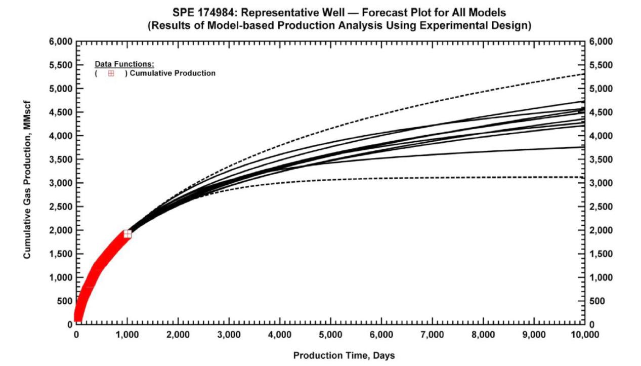
thus constrains the answer by all of the relevant physics and thus has fewer degrees of freedom in aggregate. It is true that simulation requires many inputs and that some much have large uncertainties. On the other hand, though, sits Arps decline curve analysis which has very few constraints. The history-match and then sense-check of a simulation against actual history uses the same processes as Arps, and it honors a cabinet of other parameters about the nature of the rock and the fluid which are known. Rate-transient analysis has more constraints and thus more uniqueness than historical decline analysis and it may feel more comfortable, but even RTA is constructed from a model, and that model with more simplifications than inherent to full reservoir simulation. Moreover, we can sometimes quantify the effects of the non-uniqueness. The power of new algorithms, software and hardware has enabled work processes to generate sometimes multiple history-matches, and Fig.1 is just one example showing the distribution of forecast results when multiple history-matches have been achieved. It is Interesting to note that the distributions of results are narrower than for decline curve analysis. Regardless of the inherent uncertainty, even with a single history-match or none at all, a prudent process of simulation can truly matters to our plans for the reservoir. Modeling in general and reservoir simulation in particular should not be treated as a plug-and-chug, black-box technique. It is a tool for understanding not an algorithm for an answer. Almost regardless of the outcome of the simulation, the process of deconstructing and testing the reservoir leads to greater insights and thus better development decisions. It should also not be treated as the world’s most expensive curve-fitting tool. Excessive elaboration is, in the words of Dr. Box, “often the mark of mediocrity. Less pejoratively, excessive elaboration is a rookie mistake which violates established wisdom of model-building. The insight of William of Occam has endured since the 14th-century, namely answers should favor solutions which require fewer prerequisites to be true. To find and focus on the truly key parameters, to explain the dynamics simply and elegantly, those are the requisites to a successive development campaign. In the ultimate step, simulation allows for a well or a field to be developed virtually in any number of ways before it is developed in real life. It is by far the most economical venue for experimentation and optimization in this industry without prototypes or do-overs. For sure, simulation is not the appropriate tool in every case but it probably should be used much more.

䬀唀圀䄀䤀吀

䐀攀猀瀀椀琀攀 琀栀攀 猀攀爀椀漀甀猀 挀栀愀氀氀攀渀最攀猀 漀昀 琀栀攀 漀椀氀 ☀ 最愀猀 椀渀搀甀猀琀爀礀Ⰰ 䄀䐀䔀匀 猀甀挀挀攀攀搀攀搀 椀渀 攀砀瀀愀渀搀椀渀最 椀琀猀 漀瀀攀爀愀琀椀漀渀猀 眀椀琀栀椀渀 䴀䔀一䄀 爀攀最椀漀渀 戀礀 愀挀焀甀椀爀椀渀最 渀攀眀 漀渀猀栀漀爀攀 搀爀椀氀氀椀渀最 爀椀最猀 ☀ 漀昀昀猀栀漀爀攀 䨀愀挀欀ⴀ甀瀀 爀椀最猀 椀渀 䔀最礀瀀琀Ⰰ 䄀氀最攀爀椀愀 愀渀搀 匀愀甀搀椀 䄀爀愀戀椀愀 椀渀 愀搀搀椀琀椀漀渀 琀漀 椀渀琀爀漀搀甀挀椀渀最 琀栀攀 ǻ爀猀琀 椀渀琀攀最爀愀琀攀搀 䴀伀倀唀 ☀ 䘀匀伀 ⠀䴀漀戀椀氀攀 伀昀昀猀栀漀爀攀 倀爀漀搀甀挀琀椀漀渀 唀渀椀琀 ☀ 䘀氀漀愀琀椀渀最 匀琀漀爀愀最攀 愀渀搀 伀昀昀ⴀ氀漀愀搀椀渀最⤀ 猀漀氀甀琀椀漀渀 椀渀 䔀最礀瀀琀⸀ 䄀䐀䔀匀 䜀爀漀甀瀀 栀愀猀 最爀漀眀渀 椀琀猀 昀愀洀椀氀礀 琀漀 ⬀㄀ 㐀 栀椀最栀氀礀 焀甀愀氀椀ǻ攀搀 攀洀瀀氀漀礀攀攀猀 眀椀琀栀 昀漀挀甀猀 漀渀 琀爀愀椀渀椀渀最 愀渀搀 搀攀瘀攀氀漀瀀椀渀最 琀栀攀椀爀 挀愀瀀愀戀椀氀椀琀椀攀猀 琀漀 洀攀攀琀 漀甀爀 昀甀琀甀爀攀 猀琀爀愀琀攀最椀挀 攀砀瀀愀渀猀椀漀渀 挀栀愀氀氀攀渀最攀猀 愀渀搀 漀戀樀攀挀琀椀瘀攀猀⸀

Why to Model an Oil Field

Mario Pereira de Carvalho - Senior Geologist Partner, General Geology Consultants Ltd.

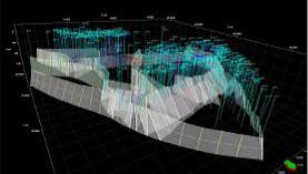
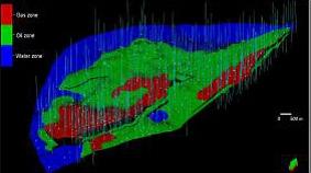
3D Geological Modeling is the best issue to visualize, in three dimensions, an oil field in its integrity.

A well-constructed 3D Geological Model allows for the visualization of all rock layers and their different geometries, the faults and displacements, relay ramps, the complex distribution of porosity, permeability, fluids, and more.

The best 3D Geological Modeling software programs have well-elaborated geostatistical interpolation and extrapolation algorithms, derived from Kriging.

The South African Mining Engineer Daniel G. Krige, along with the French Mathematician Georges Matheron, developed the Kriging process in the 1960s. Although their intent was to apply it in mining, it began to be used in E&P activities of the Oil Industry in the 1980s. Today, it is widespread in this industry.

Kriging is a regression method used in geostatistics to interpolate and extrapolate data. It assumes that the correlation of a variable with its point of origin (real data) becomes weaker with distance, and may even disappear.

Simply put, what Kriging does is to estimate, many times over, unknown values between and beyond known values (real data), using the real values as calibrators, until the average of the errors (deviations between real values and estimated values) is null, at which point the solution has been reached.

Kriging is considered a BLUE (Best Linear Unbiased Estimator) type method: it is Linear because its estimates are linearly weighted combinations against the real data; it is Unbiased because it seeks that the average of the error to be zero; and it is the Best Estimator because the estimation errors have minimum variance (estimation variance).

The application of 3D Geological Modeling in the petroleum industry is more reliable than in the mining sector because of the greater volume of data generated during the E&P of petroleum, which, in this case, are seismic and electric logs from the drilled wells.

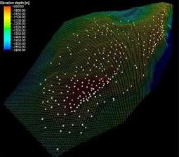
A conventional 3D seismic survey for reservoir development usually generates one seismic input every 20 meters along the surface of the reservoir layer, and the electric logs of the wells generate vertical information every 20 centimeters. For example, in an oil field with thirty million cubic meters VOIP, 100 drilled wells, two different reservoirs layers distributed in an economic target section measuring 400 meters thick, 2,500 meters length, and 1,500 meters width, and which is integrally surveyed by 3D seismic, will contain 375,000 seismic data points at the surface of the two layers, and 600,000 electric log data points generated by gamma ray, density and resistivity electric logs, totaling 225 billion inputs!

Is there another way to work and take advantage of this volume of information?

2D models do not take advantage of all of this valuable information.

The best knowledge about the structural geology of the oil field can be achieved applying the 3D Geological Modeling process, since seismic trace, for example, has a maximum resolution of around 30 meters that does not define faults with displacements smaller than this magnitude. Additionally, drilled wells, which depend on their horizontal spacing, that are almost always of the order of several tens of meters, do not define small structures either. Thus, faults with displacements smaller than 30 meters usually go unidentified, greatly reducing the satisfactory management of the flows—production and injection—and the results of infill drilling.

However, when this large amount of data is correctly manipulated in 3D Geological Modeling, all these geological structures can be visualized.

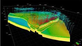
Additionally, the information provided by electric logs, cores, and other analyses from analogous oil fields allows the elaboration of 3D Geological Models of Petrophysical Attributes, such as porosity, permeability, and oil saturation—thus taking advantage of another geostatistical function offered by the software (viz. Co-Kriging) when an attribute is modeled from the spatial distribution of a different attribute.

Last, but not least, is the application of the Numerical Flow Simulation, which incorporates new attributes to the 3D Geological Model, such as Qo, Qw, Qg, GOR, relative permeability curves, compressibility, etc. and dynamically activates the 3D Geological Model trough the time, making it possible to extrapolate the future flows behavior and optimizing the reservoir oil field management.

My experience with 3D Geological Modeling started at Petrobras S.A., in 2005, where I elaborated twenty-three 3D Geological Models of Oil and Gas Fields in the Campos and Reconcavo basins, with about two thousand wells drilled.

I won the National Petrobras’ Prize PRI 2011 - Prize of Recognition and Incentive, for my contributions in the activities of the 3D Geological Modeling Process.

Step 1 – Wells and Electric Logs Download. Step 2 – Well Tops and Seismic Data Download.

Step 3 – Fault Modeling.

Step 5 – the Last Step of the 3D Grid Construction. Step 4 – Cells Size Determination.

Step 6 – Lithological Modeling.

Step 7,8 – Petrophysical Modeling. Step 9 – Fluids Modeling.

Step 10 – Upscaling for Flow Simulation.

Step 11 – 3D Geological Model Upload.

Are You Getting the Results You Want?

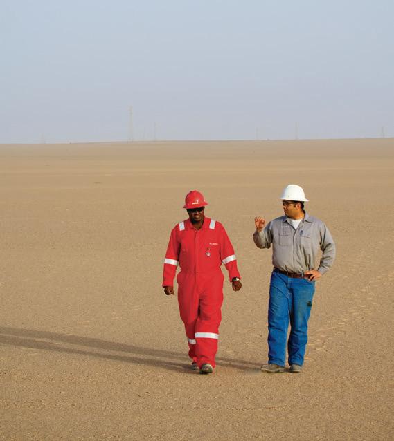
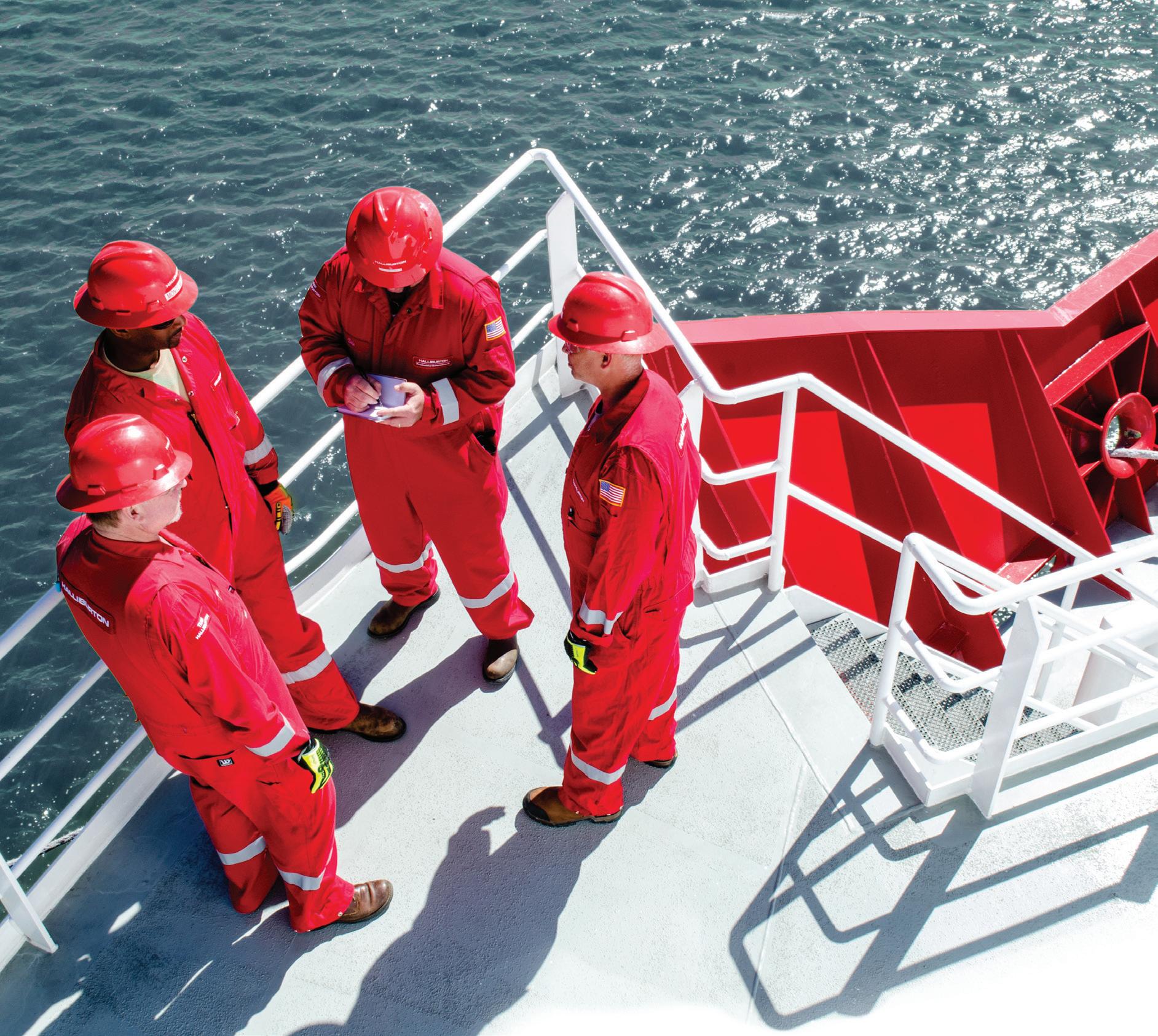
WE CAN ACHIEVE THEM, TOGETHER Whether your focus is deep water, mature fields, or unconventionals, Halliburton experts will work with you every step of the way to help maximize recovery, increase operational efficiency, and lower your cost per BOE. That’s not an empty promise. That’s our commitment to you.

Halliburton Conquering Unconventionals through Collaboration and Technology

As the world’s energy needs continue to rise and more countries pursue greater degrees of energy independence, the new frontier of unconventionals will continue to expand. The success of unconventionals across North America will find greater footing in the Middle East and North Africa. The exploration, development and production of unconventional resources are highly variable and require a collaborative, holistic understanding of the subsurface and the reservoir. Enhanced recovery techniques, such as hydraulic fracturing, combined with innovative technologies can optimize well placement and well design, identify sweet spots and improve fracture treatment and spacing to get more production at the lowest cost. Halliburton’s expertise in unconventionals spans decades as it collaborates with customers to engineer solutions that maximize asset value and lower the cost per barrel of oil equivalent. This objective is realized by accelerating reservoir understanding and reducing uncertainty through subsurface insight, developing fluids to increase drilling efficiency and well productivity through customized chemistry and delivering reliably and efficiently at the wellsite while reducing the environmental footprint. FracInsight® analysis, a workflow that leverages the best available horizontal well data to select perforation clusters and stage locations, is one of the technologies that play a significant role in developing high performing wells. It is designed to create a more consistent fracturing operation by eliminating the fracturing of nonproductive rock and predicting how the reservoir will respond to stimulation. The service is especially valuable in new and undeveloped unconventional assets that often require operators prove reserves without the expense of drilling dozens of wells to establish a learning curve. Technologies like FracInsight that draw on basin specific data are critical to driving better producing wells at lower costs. Accurate well placement is another challenge in unconventional reservoirs. Halliburton developed the Radian™ Azimuthal Gamma Ray and Inclination Service, a geosteering solution that provides real-time, high-quality borehole images and continuous inclination measurements, to help operators accurately place the wellbore in the sweet spot for increased production and lower costs per BOE. Radian recently helped an operator identify previously unseen differences between formation layers to provide a much clearer understanding of the geological structure and position of the well. This resulted in cost savings by avoiding more expensive logging while drilling technology on the job. Companies expanding their unconventionals presence across the Middle East and North Africa must also overcome the unique challenges they face. Due to the need for long horizontal drilling in the region, and the challenges this presents, Halliburton designed the Geo-Pilot Duro Rotary Steerable System to increase drilling efficiency with a higher rate of penetration. New drilling motor technology has also enhanced reliability so operators can drill longer runs while reducing costly non-productive time resulting from motor failure. As demonstrated in North America, unconventionals hold great promise and technologies that help reduce uncertainty and increase production are critical to their success.