Predictive Dissolution Modeling –Driving Towards Real Time Release Testing



Presenter: Tessa M. Carducci, PhD (she/her)
Disso America 2022

SPDS
Dissolution Science: Principles and Applications Westborough, MA Session 3: Understanding of Dissolution Mechanism to Guide Robust Formulation Development September 20, 2022 10:00 –10:30 AM EST Q = 80% in 20 minutes
Overview of talk


Role of modeling in mechanistic understanding and identifying factors that impact dissolution
Intro to in vitro predictive dissolution modeling (PDM) for drug product release

Development of a PDM for release of a drug product

2
Role of modeling in mechanistic understanding and identifying factors that impact dissolution

3
Types of dissolution modeling in the realm of predictive technology


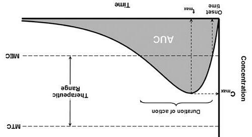
Formulation and manufacturing process Drug product dissolution performance In vivo response In vitro predictive dissolution Process monitoring in continuous manufacturing Critical materials attributes (CMAs) Critical process parameters (CPPs) In vitro–in vivo correlation/relationship (IVIVC/R) Physiologically-based biopharmaceutics model (PBBM) Q = 80% in 20 minutes 4
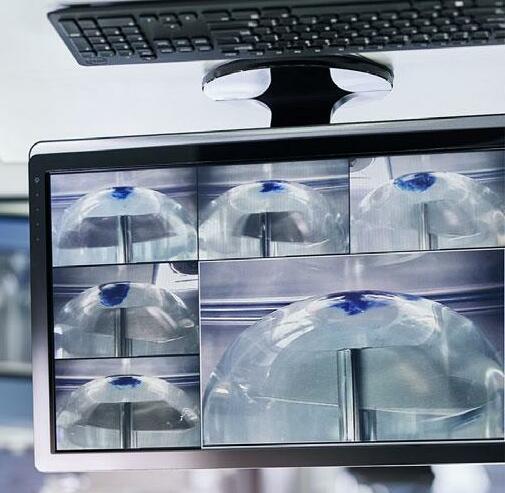
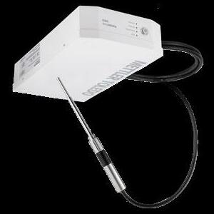
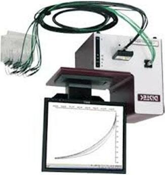
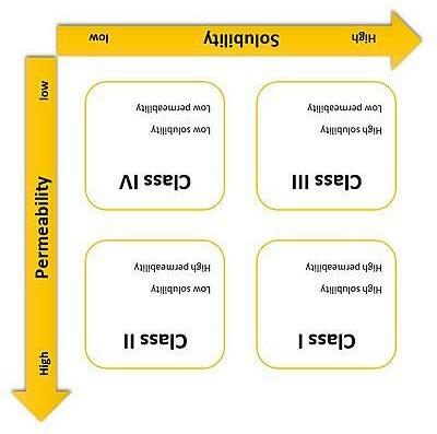
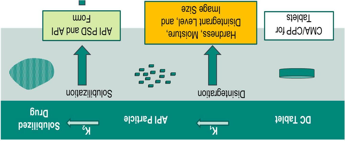
BCS II/IV likely to be solubility rate limited

5
First
modeling approach

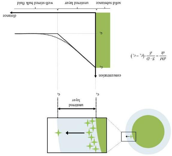
Nernst-Brunner
principles
~20 µm 1904:
Equation Fick’s 1st Law: ���� ���� ���� ���� �� �� �� Dissolution dependent on: • Solubility • Surface Area • Stirring / Agitation • Temperature 6 Mathematical modeling of drug dissolution -ScienceDirect
Case example using first principles modeling to test dissolution mechanism understanding
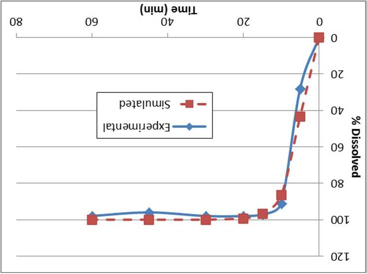
• Parameters that are likely to impact dissolution: API particle size and media pH
• Modeled according to first principle models (NernstBrunner, DDD+ Software)
• Simulated results compared to dissolution experiments of tablet DoE made with 3 different API PSD in different pH media
• Ensured the DoE would be foundational to future multivariate modeling efforts by including additional measurements, e.g. NIR, hardness, and disintegration
7 pH 1.2
Nernst Brunner Modelusing DDD+
Early stage multivariate modeling
Regression using Weibull Model
of
on
8 8 • Non-linear
• Dependence
dissolution
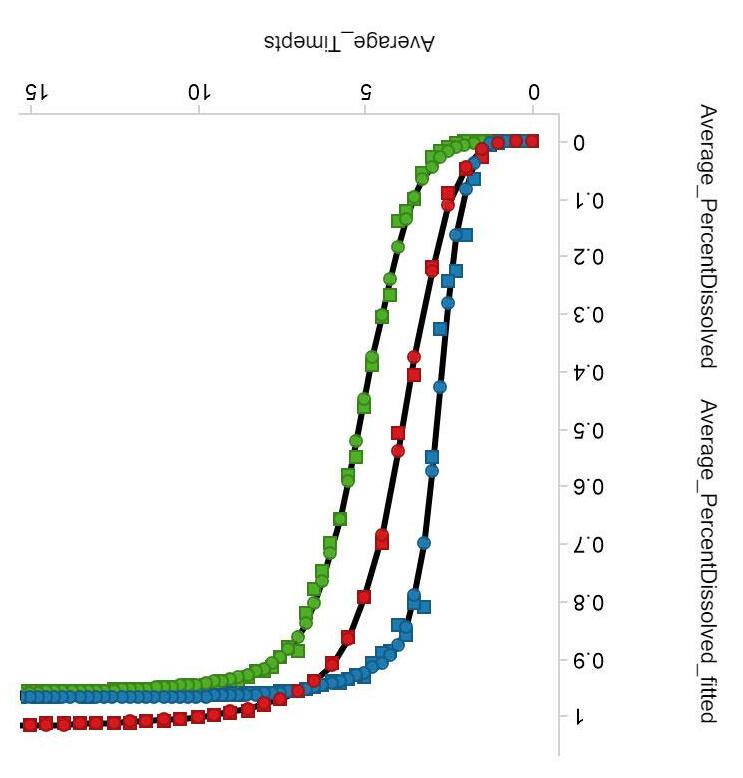
compression force is evident • Dissolution predictors could be confirmed through model crossvalidation 0 10 20 30 40 50 60 70 80 90 100 05101520 % Dissolved time (min) Run7200mpaActual Run7200mpaWeibullfit run7300mpaActual Run7300mpaweibullfit ∅ �� 1 exp �� ��
Learnings for dissolution mechanistic understanding
Need multivariate model that uses training set
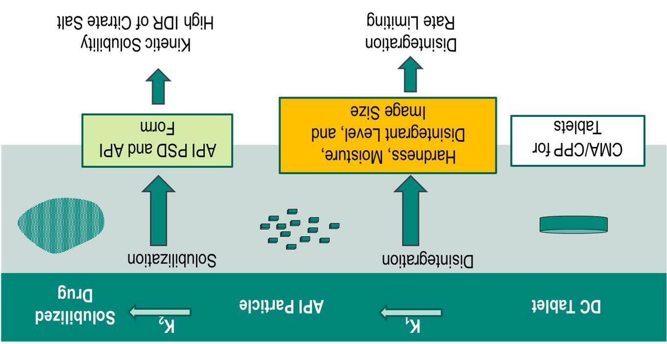
• Although tablet is BCS IV the dissolution is rapid across pH exhibiting “pseudo-BCS III” behavior
• First principles model used equilibrium solubility measurement so failed to predict the rapid dissolution in pH 6.8
• Addition of apparent solubility measurement into the model increases prediction accuracy but does not incorporate CMAs/CPPs
• Rate limiting step in this case is disintegration meaning that compression force and other scale effects are likely to play a significant role in the prediction of
dissolution response
9
Fishbone diagram for dissolution performance understanding
Blending Compression
Blend uniformity
Extent of blending
Tablet weight Blending sensitivity
Compression force
Tablet hardness
Blend physical properties
Tablet relaxation
API concentration Dissolution
Tablet temperature
API physical attributes
Water activity
Excipient physical attributes
Weight gain
Raw Materials
Film Coating
10
Intro to in vitro predictive dissolution modeling (PDM) for drug product release
11
What is in vitro predictive dissolution modeling (PDM) for release?
2012 Q8, Q9, and Q10 Q&A FDA guidance for industry
•“…a multivariate model (e.g. a partial least squares (PLS) model), when appropriate, can be used as a surrogatefor traditional dissolution testing. In this case, the PLS model should be developed in terms of inprocess parameters and material attributes and can be used to predict dissolution.” -
EMA’s 2012 “Guideline on Real Time Release Testing”
•“Attributes relating to the properties of a tablet granule such as porosity, particle size, surface area, bulk/tapped density etc. if shown to have a predictive relationship with dissolution behaviour could serve as RTR testing surrogates for dissolution testing. These dependencies would have to be confirmed on a productby-product basis.”
•“Predictive dissolution modeling is an emerging methodology defined as the ability to mathematically generate a time profile of the dissolved amount of an API based on information regarding material properties, dissolution method conditions, formulation composition, and process parameters.”
IQ Workshop Summary Report, 2022



•First-principles and empirical approaches to predicting in vitro dissolution for product release testing…predicting a quantitative value of the level of drug released at a specific time point, as is done traditionally with a physical dissolution test.
 AAPS Whitepaper 2019
12First-Principles and Empirical Approaches to Predicting In Vitro Dissolution for Pharmaceutical Formulation and Process Development and for Product Release Testing | SpringerLink http://dissolutiontech.com/issues/202208/DT202208_A04.pdf
Can we implement RTRT for any/every product?





Immediate release
BCS class I or III
Very stable (no degs)
Drug loading Dev. timeline constraints
Global regulatory acceptance

Real time release testing scheme for non-BCS I/III drug product
API Blend Lubricant Blend Compress Film coat Rapid Release Testing Manufacturing Floor NIR ID Appearance Manufacturing Floor NIR Composite Assay NIR Content Uniformity Traditional Release Approach Laboratory Lab Tests HPLC Content Uniformity Composite Assay Degradates Identity Dissolution Appearance Lab Test Dissolution RTRT Manufacturing Floor Addition of Dissolution Model for release to replace lab test 14
(current)
(future)

peak volume, RTRT has 34% FTE savings benefit incremental to Rapid Release

What is the value of PDM? 0 1 2 3 4 5 6 7 8 9 10 202120222023202420252026202720282029203020312032203320342035 FTE Savings Year Rapid Release
RTRT
At
21 4 0 0 1 1 9 9 9 0 5 10 15 20 25 30 35 Baseline ProductRapid ReleaseRelease with Predictive Dissolution CALENDAR DAYS Testing/Release Cycle Time/Batch Lab Testing Shop Floor Testing QA Review FTE Savings Inventory Savings+ Total USD savings= 15
Batch
-Large, centralized facilities
-Few campaigns in large batches
-Large inventories
Continuous
-Agile facilities
enables flexibility
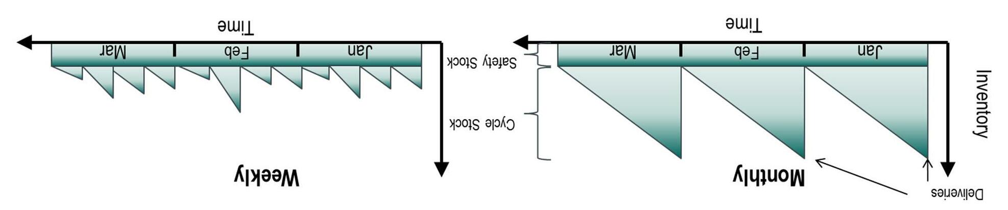
-Many campaigns with quick turnaround -Smaller inventory
To realize full benefits of continuous manufacturing, RTRT is imperative
RTRT is required to keep up with batch release!
16
for release yields strategic and business benefits
business drivers
RTRT to low solubility
PDM
Extends
for
products Typical drug product candidate for RTRT is BCS I or III (high solubility) “Rapid release” strategy will not realize full benefits Enabler of CM strategy for BCS II/IV Avoidance of wet lab dissolution testing Safety and compliance Digitization and data integrity Decrease or streamline dissolution related investigations in supply Enhanced dissolution mechanistic understanding Dissolution mechanism and kinetics Identifying dissolution sensitivities and CMAs/CPPs Troubleshooting support 17
Overview of developing a PDM for release
Early development
Latedevelopment
Validation and implementation
mechanistic understanding of dissolution response
dissolution sensitivities through small scale
QC method selection justification is strong
materials risk assessment
through
dissolution
dissolution method robustness and minimize unwanted variability
regression between
response
the
maintenance
18
~FIH to IIb •Gain
•Investigate
DoEs •Ensure
•Raw
~Ph III to FSS •Confirm
sensitivities
scale‐up DoEs •Optimize
•Multivariate
predictors and
dissolution
Prior to PPQ •Model cross validation and evaluation of independent data •Control strategy and implementation •Site readiness and
plan
Development of a PDM for release of a drug product
19
Dissolution performance
specification strategy
•
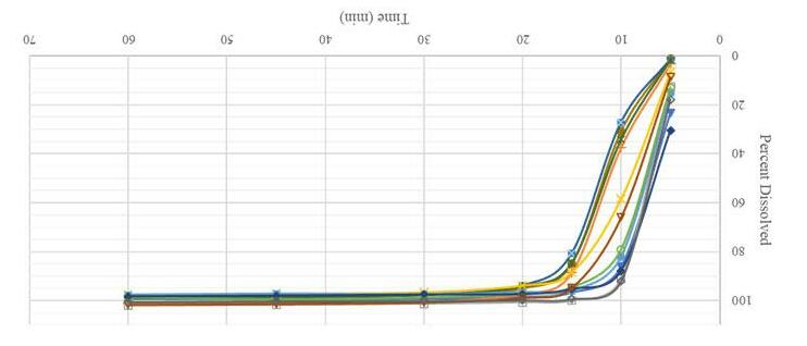
dissolution method: 100 rpm baskets, pH 6.8
Q = 80% in 20 minutes
Time(min)
model strategy
BCS IV but relatively fast dissolution due to high apparent solubility of the API across pH
• Supersaturation in pH 6.8 disso media stabilized by HPMC in the formulation
• Dissolution is sensitive to tablet hardness, and %RH at early time points
Method is discriminating for API form as exhibited by lower plateau region in presence of freebase
Initial lag time due to film coat removal but has little/no impact at Q time point
Early time points have high variability
•
•
•
0 20 40 60 80 100 0102030405060 Percent Dissolved
Proposed
QC
20
strategy for

0.0 20.0 40.0 60.0 80.0 100.0 120.0 0.002.004.006.00 Dissolved (% Label Claim) Time (Minutes) Predicted vs Measured End to end
predictive dissolution modeling Empirical or Hybrid Model Design of Experiments (Predictors) 0.0 20.0 40.0 60.0 80.0 100.0 120.0 0.005.0010.00Dissolved (% Label Claim) Time (Minutes) Predictors NIR data Dissolution Profiles Routine Use Routine Verification Periodic VerificationIf needed Model Update Re-validate model Routine Use in Supply Curve fitting for dissolution profiles e.g., Weibull curve fit % ���� �� 1 exp Step 1 Regress the parameters of curve fitting in Step 1 against predictors and NIR data (e.g., PLS, nonlinear regression) �� �� �� , �� , �� ,…, ������ b �� �� , �� , �� ,…, ������ c �� �� , �� , �� ,…, ������ Step 2 21
Fishbone diagram for dissolution performance understanding
Blending Compression
Blend uniformity
Extent of blending
Tablet weight Blending sensitivity
Compression force
Tablet hardness
Blend physical properties
Tablet relaxation
API concentration Dissolution
Tablet temperature
API physical attributes
Water activity
Excipient physical attributes
Weight gain
Raw Materials
Film Coating
22
PDM DoE at commercial scale, sampling strategy, and data aggregation
• Parameters: API size, blending and lubrication, film coating conditions, compression conditions, and film coating weight gain
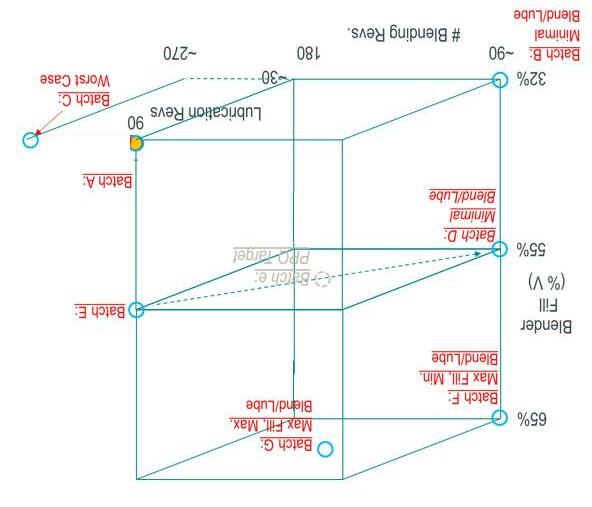
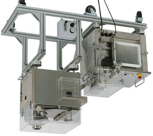
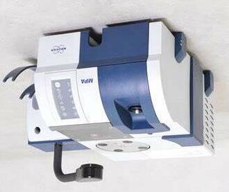
• Scanned tablets by NIR for %LC and spectral information before dissolution
• Measured tablet weight, thickness, and diameter before dissolution
• Utilized Spotfire platform to combine dissolution and process data together
23
Y-block, and model selection strategy
X-block,
24 • Single time point modeling -exploratory analysis Build understanding how/which process conditions affect various timepoints of dissolution profiles, spanning early timepoints to Q. Multivariate regression of process parameters (X) and % dissolved at various single time points (Y) Utilized set of relevant process data and early dissolution timepoints at 5 –15 minutes • Full profile modeling –iterative process towards final model Develop a multivariate model based on process conditions (X) and disso profile fit coefficients (Y), where the fit coefficients describe the full dissolution profile Evaluate fit equations and compare model rank and condition number Evaluate effect of low resolution dissolution with 6 time points vs. high resolution fiber optic profile Parameters that do not significantly impact dissolution performance can be excluded from X block
Variance in the dissolution data is systematic and/or random
Early time points in profile are highly variable, expected to be more sensitive to systematic process and environmental conditions
R2 is a measure of the percentage of variance captured by the model
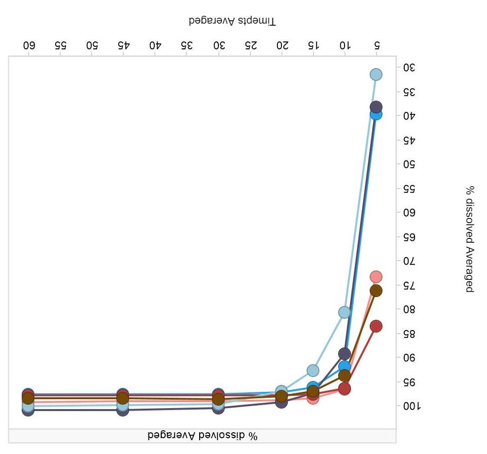
Later time points have less variance (both systematic and random)

25
Exploratory analysis: regression at 5 min dissolution timepoint
Loading plot (shows directionality of impact)
% dissolved (measured) vs % dissolved (predicted)
Predicted vs. measured shows high (~90%) of variance explained by model
26
Exploratory analysis: regression at 10-and 15-minute timepoints
% dissolved (measured) vs % dissolved (predicted) @ 10 min
% dissolved (measured) vs % dissolved (predicted) @ 15 min
Predicted vs. measured at later time points shows high accuracy but lower % of variance explained (as expected)
27
Preliminary model X-block
Core tablet weight

Correlates with API conc. for DC process






Encompasses impact of moisture
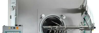
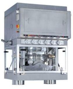
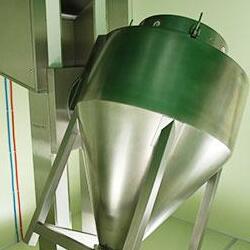
comp force
Encompasses impact of API PSD, fill depth, etc.
Hardness
Main
28 Batch size, blending revs, and lubrication revs Blending K Film coat lag time at early time points FC weight gain API concentration NIR
Model the full dissolution profile via fit coefficients
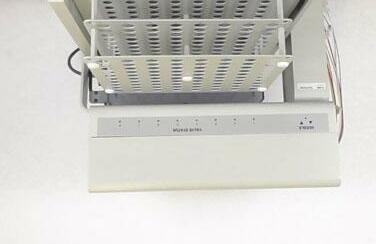
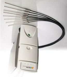
Low resolution
Whitney
High resolution
Gompertzequation

0 20 40 60 80 100 051015202530 %Dissolved Time (min)
Three models were evaluated against full scale DoE at commercial site: Modified Noyes
framework ∅ �� 1 exp ���� , �� �� 1 exp �� �� Weibull equation ∅ �� 1 exp �� ��
∅ �� exp exp �� �� ��
29
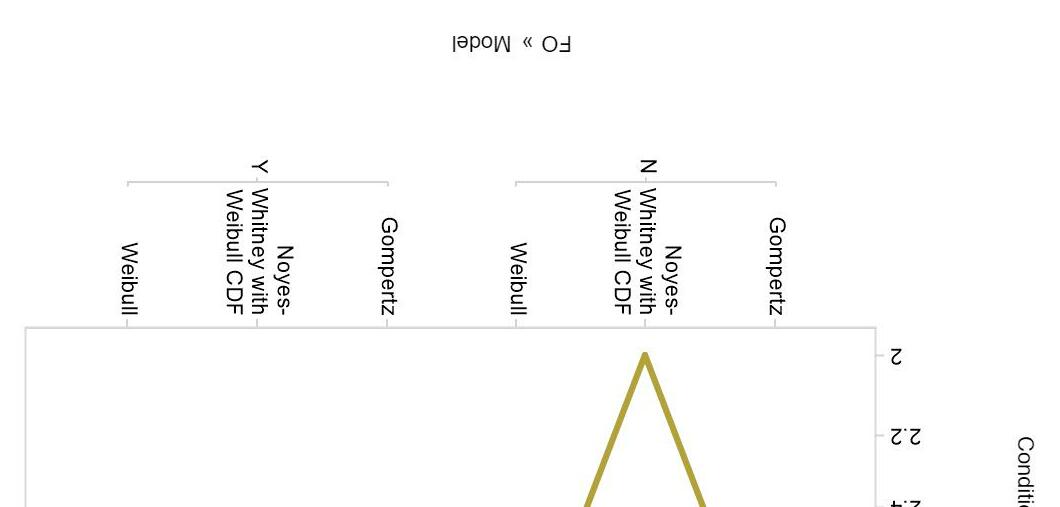
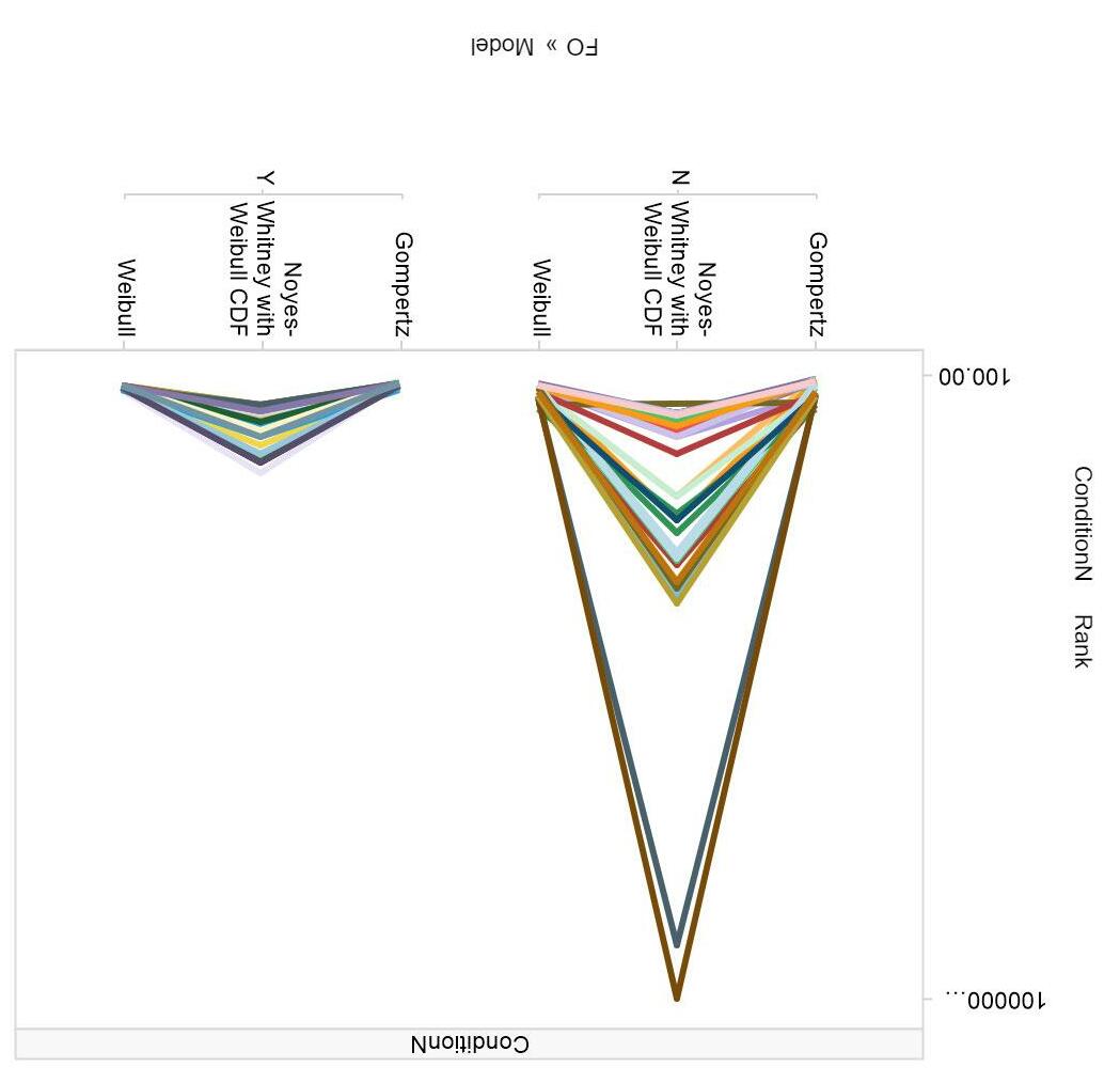
Model options analysis based on technical performance
Rank of FIM ⇒ number of parameters that can be uniquely estimated (measure of correlation)
Condition Number of FIM ⇒ indirect measure of accuracy, measures if the matrix is ill-conditioned
ModelLow resolutionHigh resolution
MNWVery high condition number
Inconsistent rank across the design space

Weibull Very low condition number
Consistent rank (= the number of total parameters)
Gompertz Very low condition number Consistent rank (= the number of total parameters)
Relatively higher condition number (higher covariance expected) Consistent rank (= the number of total parameters)
Very low condition number Consistent rank (= the number of total parameters)
Very low condition number Consistent rank (= the number of total parameters)
•
• Low resolution data preferred for ease of model maintenance in supply
• Not possible to estimate all the parameters in MNW model using low-res data
Gompertz model explained the disso profile better especially at approach of the plateau region
30
Step 1 Model: Demonstration of model via fit equations
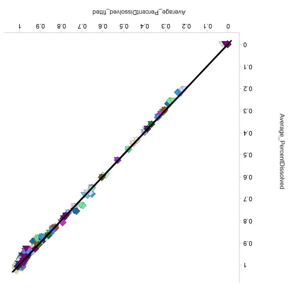
Step 1 –Apply the fit equation model through a set of lab dissolution (low res) profiles
Comparing the Gompertz fit vs actual % dissolved Gompertz equation
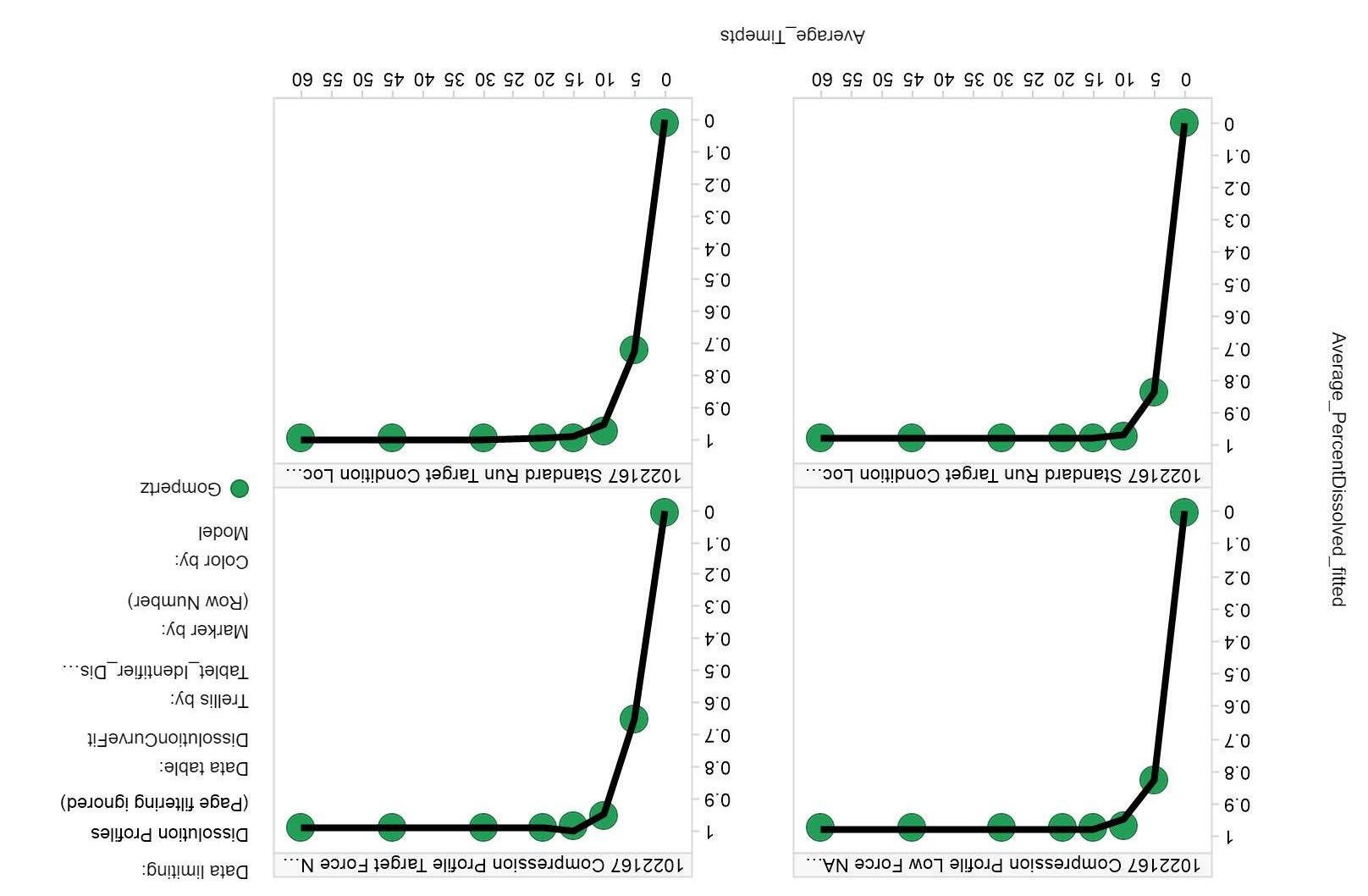
R2 = 0.99
∅ �� exp exp �� �� �� 31
Regressing disso curve parameters against process conditions
DissolutionStep2Model_May2022.M8 (PLS), Gompertz k1 - old
according to Obs ID (Batch Identifier)
block
5.413e-008
0.5166
Compression Force
Depth
K
DissolutionStep2Model_May2022.M9 (PLS), Gompertz k2 -
according to Obs ID (Batch Identifier)
block
1.988e-007
32
X
Colored
y = x +
R2 =
0 0.2 0.4 0.6 0.8 1 00.20.40.60.81 YPred[2](0) RMSEE = 0.155783 RMSEcv = 0.157744 Batch A Batch B Batch C Batch D Batch E Batch F
old X
Colored
y = x +
R2 = 0.7532 1 2 3 4 5 6 7 8 12345678 YPred[3](1) RMSEE = 0.760027 RMSEcv = 0.758435 Batch A Batch B Batch C Batch D Batch E Batch F Gompertz: �� exp exp �� ∗ �� �� Process Parameters: Tablet Weight Tablet Hardness Main
Fill
Blending
Step 2 Model:
Step 2 Model: Regressing disso curve parameters against process conditions
Parameters:
Weight
Weibull: �� 1 exp
Hardness
Compression Force
Depth
K
DissolutionStep2Model_May2022.M6 (PLS), Weibull k1 - old X block Colored according to Obs ID (Batch Identifier)
= x + 7.765e-008 R2 = 0.4912
= 0.431989 RMSEcv = 0.433865
B
C Batch D Batch E
A
DissolutionStep2Model_May2022.M7 (PLS), Weibull k2 - old X block
Colored according to Obs ID (Batch Identifier)
= x + 5.06e-007
= 0.7305
F
= 1.35908
= 1.36993
A Batch B Batch C Batch D Batch E Batch F
33
y
0.5 1 1.5 2 2.5 3 0.511.522.53 YPred[2](0) RMSEE
Batch
Batch
Batch
Batch
y
R2
0 2 4 6 8 10 0246810 YPred[2](1) RMSEE
RMSEcv
Batch
Process
Tablet
Tablet
Main
Fill
Blending
Predicted vs. measured for calibration training set
Red –Measured
Black –Predicted
Average residual is 1% and most predicted dissolution results at spec time point are within 3% of the lab dissolution result
34
Next steps for model validation and implementation
Refine model development
analysis
quantification
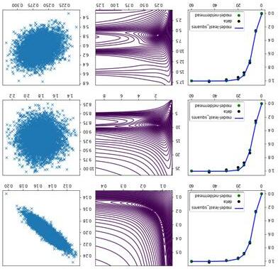
x-block (iterative)
Model operationalization & maintenance
Model validation strategy
•Based on classical validation elements
independent data
there is consensus in field that validation is only needed for Q timepoint
Use
Verification
•Residuals
•Uncertainty
•Revisit
•Cross-validation •Evaluate
•Generally
Routine
Routine
Periodic VerificationIf needed Model Update Re-validate model 35
Can we build a model using scale independent parameters?
Scale –dependent
Main compression force
Hardness
Blending constant
NIR (%LC)
Core tablet weight
Film coat weight gain
Scale –independent

Hardness
Bulk/tapped density
NIR (%LC)
Core tablet weight
Film coat weight gain
Pros: Likely to be lower cost for development and model maintenance, can use small scale equipment so does not need to take up time on manufacturing site equipment, more easily able to do batch perturbations at development site to push towards failure points
Cons: Parameters may not be equivalent, model may not be as robust, and parameters may not always be easier to measure
36
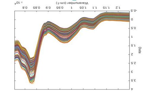
Alternate modeling approach: spectrum-based (PAT-based) model
NIR classification model has shown distinction between slower dissolving batches
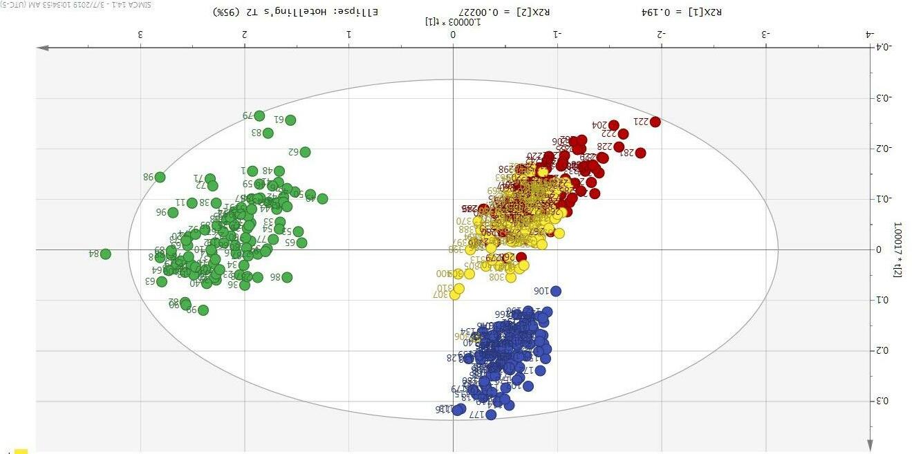
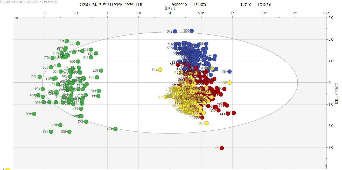
Pros: NIR spectrum is a tablet measurement –no need to regress process parameters, measurement is applied to the final product which gives more confidence in product quality
Cons: Phenomena being measured may not always be understood or may not be meaningful
37
for a batch versus a continuous process:
PDM
Commercial scale blending & dissolution study (6) Blender Steady States (SS) (21) Feed Frame (FF) & Turret Speed Steady States (5) Hardness samples per blend SS (1) Hardness samples per FF SS (6) Film Coating Conditions Batch: 6 batches totaling 2060 kg of blend ~$200k in API cost Blending/lubrication design along with varying press parameters 2+ weeks of manufacturing If executed as a continuous study: 150 -300 kgs depending on executional efficiency < 1 week of manufacturing 38
Open questions –#1
How does sampling and assessing against the specification work for PDM?
Dissolution models for release previously approved by FDA followed USP <711> using N = 12 tablets and assessing against Stage 2 acceptance criteria.
Following USP <711> will allow for most alignment between lab disso and disso model sampling and result assessment and will also make model maintenance more straightforward
Another possible approach is to use a statistically-based assessment criteria with a larger number of replicates
This approach may make more sense for continuous processes where large(r) N is needed
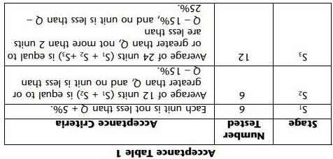
Additionally, RSD at Q timepoint for this product is low and does not necessitate an increased number of replicates.
•
•
•
39
Open questions -#2
How to show discriminatory power of the PDM model?
• Dissolution model are expected to be as sensitive as the lab QC dissolution method especially for CMAs/CPPs
• For multivariate models, the model inherits the variance (discrimination power and random variability) of the lab QC dissolution method because the model is trained using real data as input.
• The dissolution mechanism and method selection are important foundations to model development. For a multivariate model, changing the QC dissolution method would render the model training set basically useless.
• Need to ensure that the input data covers the various dissolution dependencies that exist and incorporates many potential sources of variation in the inputs (i.e. raw materials attributes).
• Ability of PDM model to detect specification failure is very important either using a real batch (ideal) or by using a virtual batch as input.
• In routine supply, the model can be updated with more data as more variation of inputs are seen.
40
Open questions –#3
How are lab dissolution and PDM results handled when generated simultaneously?
There are scenarios where both lab dissolution results and model results will be generated for the same batch i.e. during routine parallel testing for model maintenance or for countries that do not have the disso model filed/approved
Lab dissolution may also be run shortly after the model prediction as post release testing (i.e. TOI or stability T0) by downstream sites.
How will we gauge if model and lab results are aligned? Do we need to?
Define when assessment needs to be performed in the quality system
Use a sound statistical approach (i.e. 95% CI) and/or follow method transfer criteria (i.e. % dissolved at Q is within +/-5%)
Having f2 or other profile similarity criteria is not ideal because a dissolution profile is not routinely measured for release by lab
What happens if the lab disso result does not align with the result predicted by the model? Model maintenance will be triggered and involve updating the model.
•
•
•
41
Open questions –#4
How close are we to global acceptance of PDM for release?
• There are several successful examples of PDMs for release approved in US, EU, and possibly other markets.
• There was recently a new MFDS (Korean agency) regulation on RTRT for new products that mentions predictive dissolution modeling.
• Our efforts to influence regulatory guidelines and put forth innovative filing applications for new products will pave the way for future programs with RTRT strategies towards global acceptance.
• Can be used in combination with physiologically-based biopharmaceutics modeling (PBBM) to support clinically relevant justifications. Building clinical relevance into RTRT can help strengthen package and boost chances of regulatory acceptance.
42
Overall summary and conclusions
•
Mechanistic understanding matters for dissolution method selection, justification, and to lay a foundation for future commercial release strategies
• Investment in modeling to understand dissolution mechanism may prove useful in investigations down the line
• Predictive dissolution modeling for release can be a key enabler for RTRT and CM strategies for low solubility drug products
• Although there are already successful approvals for use of predictive dissolution modeling for release, it is still a relatively new regulatory concept that will benefit from pharmaceutical companies pushing the envelope by filing innovative strategy proposals globally for model validation, assessment, etc.
43
Acknowledgements
Contributors & supporters
Nathan Pixley
Jasdeep Mandur
Andre Hermans
Leah Xiong
Kevin Reuter
Anushka Gupta
Diana Watkins
Chitra Telang-Lobo
Kevin Reuter
Plinio de los Santos
Chris Pridgen
Courtney Stanton
Azzeddine Lekhal
Brandye Smith-Goettler
Plamen Grigorov
Andrew Buss
Shailesh Singh
Mano Ramasamy
Asha Rajapakshe
Krista Witkowski
•
•
•
•
•
•
•
•
•
•
•
•
•
•
•
•
•
•
•
•
44
Thank you!