1 Technical feasibility of biogas production

1.1 Introduction to feasibility study

Singh Farming and Griffith University have identified surplus sugarcane bagasse (20,000 t/a) and mill mud (30,000 t/a) as potential feedstocks for anaerobic digestion (AD) with locally sourced chicken manure (5,000 t/a) to generate biogas (i.e., codigestion). In addition to biogas, the AD process would also produce a nutrientrich digestate. The digestate can be pasteurised and separated into solid and liquid fractions. The solid fraction would be sold as a soil conditioner/organic fertiliser while the liquid fraction would be recycled as process water in the AD plant.

To assess the feasibility of the proposed project, different scenarios were designed with an aim to evaluate the possible market opportunities for biogas uses and the overall return on investment (ROI) it generates Scenario development is important to determine the outcomes of project development in a context that is relevant for stakeholders. Further, the studied scenarios will also help in the process of decision-making. Based on the biogas usage, three different scenarios were considered in this feasibility study and are presented in Table 1.

• Scenario 1: CHP Biogas is used for electricity and heat generation in a combined heat and power (CHP) plant.

• Scenario 2: CHP + BioCNG A portion of biogas is used for CHP to generate electricity and heat to meet the parasitic demand of the biogas plant and the remaining biogas is upgraded and compressed (BioCNG) for vehicle fuel or distribution via virtual pipeline (road transport)

• Scenario 3: CHP+ BioRNG—Similar to Scenario 2 but the biogas is upgraded to renewable natural gas (BioRNG) for grid injection.

Under both Scenarios 2 and 3, the carbon dioxide (CO2) will be recovered and liquified to be sold as food grade BioCO2

Biogas

1.2 Drivers for feasibility study

The cost of sugarcane crop production in Queensland is increasing every year. Of the total production costs, water and pumping accounts for 15% each while diesel fuel accounts for 10%. Diesel consumption is estimated at 3 L/t cane. The high costs of water, electricity and diesel are severely limiting crop yields and farm profitability since farmers are unable to afford sufficient water at critical crop growth stages. A highly prospective opportunity to reduce energy costs is to produce biogas using sugar industry wastes, given their high energy content. By generating electricity onsite, we can reduce the retail and transmission costs by up to 50% of total electricity costs. The biogas can also be upgraded to BioCNG to replace grid-supplied electricity and diesel used for irrigation, farming, and transport.

Currently, sugar industry wastes are used for on-site energy generation in boilers, which were designed as incinerators for burning bagasse rather than recovering full energy potential of biomass. Mill mud is currently spread on farms as soil conditioner Biogas can play an important role by providing an opportunity to meet our renewable energy targets and decarbonise our economy, as well as provide a holistic solution for the sugar industry and other livestock farms and municipalities in managing their wastes. The national biogas industry is likely to expand, as there is significant potential for growth in feedstock, coupled with rising electricity prices and landfill levies.

This project will repurpose sugar industry wastes to reduce operating costs for Australian sugar farms and help them in transitioning to renewable energy.

1.3 Methodology for feasibility study

1.3.1 Plant location

The plant will be located at Mossman Sugar Mill, Mossman, Queensland

1.3.2 Biogas plant design calculations and assumptions

Techno-economic evaluation of biogas production from the studied feedstocks was performed as per the designed total electrical power output of 2.2 MW. Based on the best methane yields obtained in the biochemical methane potential (BMP) study, codigestion of sugarcane bagasse and mill mud with chicken manure was selected The biogas plant will be operated all year round with some days allocated for repair and maintenance. The plant will operate 24/7 and is expected to be equipped with sufficient instrumentation and telemetry to allow for remote access and control of the plant. An estimated operational period of 8,300 h/year was considered.

The plant will be operated as follows:

• waste streams delivered to biogas plant 7 days/week during sugarcane harvesting and processing season

• biogas generation 24/7, year-round with 95% plant availability

• BioCNG/RNG/electricity production 24/7, year-round

• power demand (where applicable) 24/7, year-round

• liquid digestate discharge 24/7, year-round

• solid digestate offtake 4–5 days/week, year-round

Table 2 shows the feedstock quantities (t/d), chemical composition and methane potentials used for the design calculations. Sugarcane bagasse and mill mud will be collected from Mossman Sugar Mill while chicken manure will be procured from Mareeba. The road transport distance is estimated to be 75 km. The methane yields used in the study were normalised to standard temperature and pressure (STP) conditions (0°C, 1 atm).

Table 2. Feedstock amounts along with their chemical composition and methane yields used for design calculations of farm-scale biogas plant.

1 TS – total solids, VS – volatile solids

2 w/w: wet weight

3 Methane yields (Nm3/kg VSadded) are calculated after being normalised to standard temperature and pressure

1.4 Biogas plant design

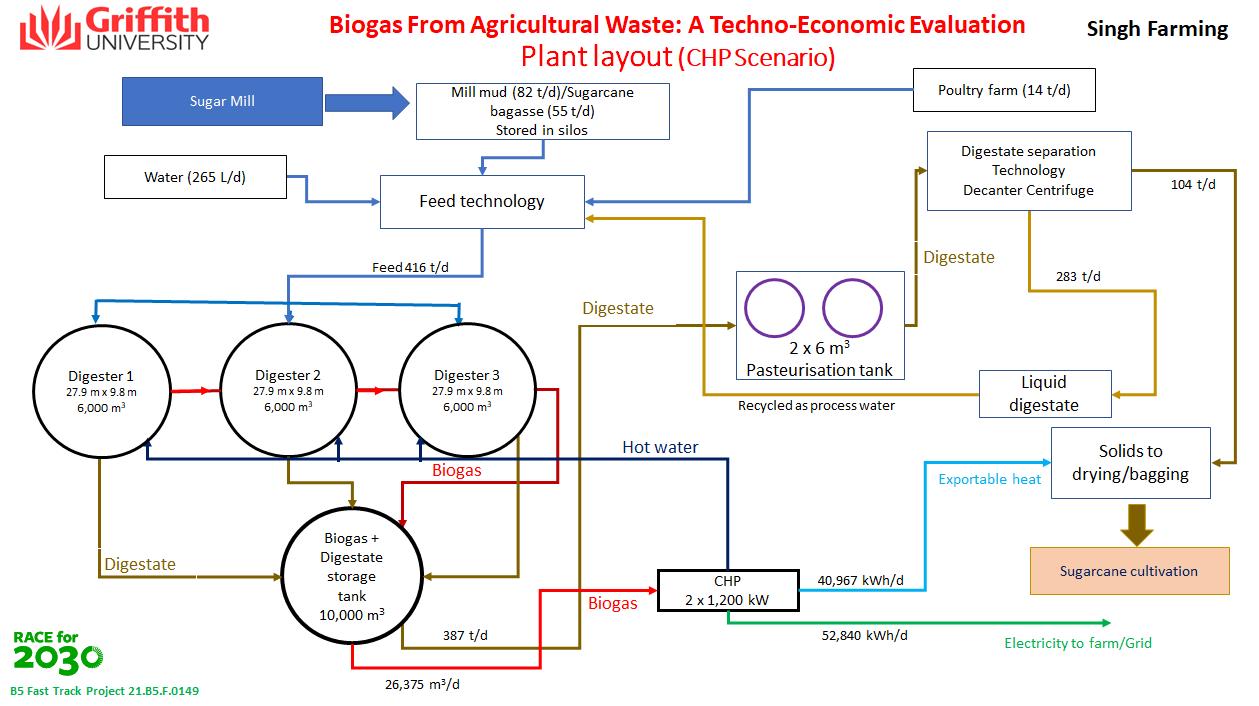
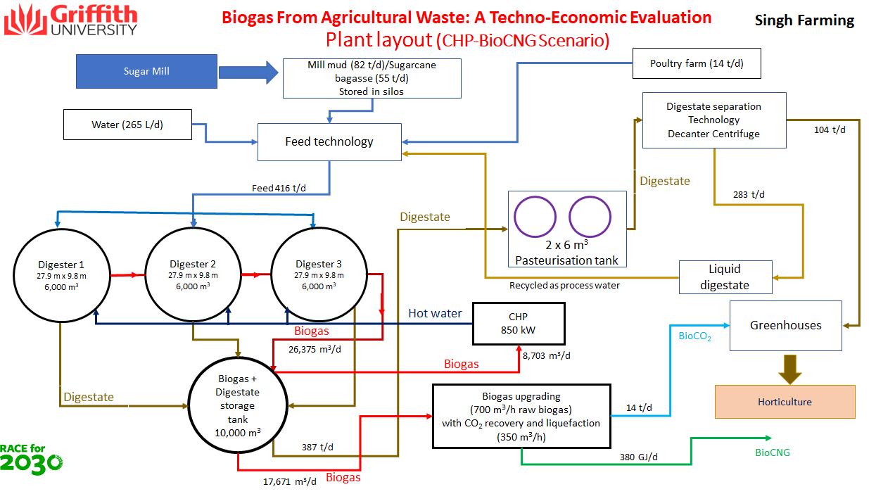
The biogas plant concept and process flowchart for CHP generation (Scenario 1) and for CHP + BioCNG with additional BioCO2 production (Scenario 2) are presented in Figure 1 and Figure 2, respectively The process flowchart for Scenario 3 is not presented as it is similar to Scenario 2, with only minor changes in biomethane use equipment. Both bagasse (55 t/d) and mill mud (82 t/d) generated during the cane crushing season (June to December) will be used as feedstock For off-season supply, biomass produced during the on-season will be ensilaged and stored as silage in concrete bunker silos. Two concrete bunker silos (10 m × 4.5 m × 2.5 m) were considered for the ensilation process. Lactic acid bacteria at the rate of 4–5% on fresh weight basis will be used. Possible storage losses were not considered in this study On the other hand, chicken manure (14 t/d) is procured from poultry farms in Mareeba

The feeding technology consists of maceration coupled with an augur feeding system and feed buffer tank. Feedstocks are macerated, mixed, homogenised and fed into the buffer tank In the buffer tank, chicken manure is added along with process water (265 kL/d) and liquid fraction of the digestate, to adjust the solids content to <8%. The feed buffer tank (2,900 m3) was designed to prepare feed for five working days (Monday through Friday). Feed rates were designed so that the feedstocks will be consumed evenly throughout the year. The prepared feed is then fed to the biogas reactors (Figure 1 and Figure 2).

Three semi-continuously stirred tank reactor (CSTR) systems (3 × 6,000 m3) were designed to enable the implementation of the proposed codigestion system in a full-scale plant. CSTR technology is widely applied in the European biogas plants for a range of residues including energy crops and livestock manure AD (Janke et al., 2016)2 . The reactors have mechanical agitators to mix the reactor contents. The rectors will be operated at an organic loading rate (OLR) of 3.3 kg VS/m3/d, hydraulic retention time (HRT) of 35 d and process temperature of 37°C. The well-insulated upright galvanised steel CSTR reactor has sufficient headspace for biogas to evolve and flow to a post-storage tank.

The biogas and digestate produced from the three CSTR reactors are stored in the post-storage tank (10,000 m3). Prior to solid–liquid separation of digestate, the whole digestate is sent to pasteurisation (2 × 6.0 m3) and carried at 70°C for 1 h to kill the zoonotic pathogens in the digestate. The pasteurised material is then separated into solid and liquid fractions by using a decanter centrifuge (48.3 m3/h). The solid fraction is sold as soil conditioner while the liquid fraction is returned as process water to dilute the incoming feedstock.

The biogas train consists of a biogas blower, desulphurisation unit and a flare. In Scenario 1, desulphurised biogas is fed to the CHP plant (2 × 1,200 kW) by a biogas blower (1,060 m3/h) to produce heat and electricity (Figure 1).

Two stationary internal combustion engines (electrical output of 899–1,500 kW and thermal output of 95–1,812 kW) with an electrical conversion efficiency of 0.424 and thermal conversion of 0.426 were used After meeting the parasitic electricity needs, the surplus electricity is fed to the grid Heat as hot water from the CHP plant is used internally for heating the reactors.

In Scenario 2, approximately 8,703 m3/d of biogas (33% of total production) is fed to the CHP plant (850 kW) to produce heat and electricity to meet the parasitic demands of the biogas plant. The remaining biogas (17,671 m3/d) is fed to a membrane biogas upgrading unit (700 m3/h raw biogas) coupled with CO2 recovery and liquefaction plant (350 m3/h) to produce BioCNG and bioCO2, respectively. The PurePac Medium biogas upgrading system (400–1,000 Nm3/h raw biogas) and CO2 recovery system, manufactured by Bright Biomethane (the Netherlands) was considered. A methane yield of 99.5% is guaranteed in this highly efficient membrane upgrading technology. A 2% BioCH4 slip was considered during biogas upgrading This reflects the worst-case scenario within the range (1–2%) usually observed in upgrading technologies (Muñoz et al., 2015)3 In case of emergency, biogas can be flared on site by using the biogas flare (539.5 m3/h).

1.5 Mass balance

Table 3 details the mass balance for the studied scenarios. For all scenarios, anaerobic codigestion of 151 t/d of the studied feedstock and 265 kL of water will produce 26,376 m³/d of biogas (30 t/d) and 386 t/d of digestate. Separation of the digestate into solid and liquid fractions by using a decanter centrifuge resulted in 104 t/d of solid fraction and 283 kL/d of liquid fraction. The solid fraction accounted for 27.16% w/w of the total digestate and had a solids content of 30% (Table 4). The liquid fraction had a solids content of 1.2%.

Table 3. Mass and energy balance of anaerobic codigestion of sugar mill by-products with chicken manure.

1.6 Energy balance

Table 3 shows the energy balance for the studied scenarios. For all scenarios, a daily biogas production of 26,376 m3/d was obtained from 151 t/d of feed. In Scenario 1, use of the produced biogas for heat and electricity generation in CHP resulted in 61,456 kWh/d of electricity and 58,304 kWh/d of heat. Considering the energetic performance in Scenario 1, the installed capacity of the biogas plant is 2.2 MW. For Scenario 2, use of biogas (33% of total production) for heat and electricity cogeneration in a smaller size CHP plant (1 × 850 kW) produced 19,797 kWh/d of electricity and 19,276 kWh/d of heat. The remaining biogas, when used for biogas upgrading with integrated CO2 recovery and liquefaction, can produce 380 GJ/d of BioCNG and 14 t/d of foodgrade BioCO2. The produced BioCNG can be used to replace fossil fuel in vehicles (Scenario 2) or injected into the natural gas grid (Scenario 3), depending on the production level and the distance to the natural gas grid. In contrast to electricity generation in Scenario 1, where heat losses usually account for over 50% of the available

‘raw energy’ (i.e., the installed capacity of the biogas plant), the energy potential of BioCNG production could reach values as high as 98% owing to the much lower energy loss levels (2% in this case).

The parasitic energy demand for biogas plants in the studied scenarios varied and was dependent on the process configuration and the plant equipment used In Scenario 1, parasitic energy demand was 8,615 kWh/d of electricity and 17,337 kWh/d of heat. This energy demand was supplied by the produced heat and electricity from onsite CHP plant. Thus, import of heat (natural gas) and electricity (grid electricity) was not required. For Scenario 2 and 3, the parasitic energy demands were relatively high (15,191 kWh/d of electricity). This high energy demand is attributed to the energy requirements of the BioCNG (4,560 kWh/d electrical) and for liquefaction of BioCO2 (2,016 kWh/d electrical) The electrical energy requirement for biogas cleaning and upgrading with compression was 0.3 kWh/m3 raw biogas (Scenario 2) and without compression was 0.22 kWh/m3 raw biogas (Scenario 3). The corresponding electrical energy requirement for CO2 recovery and BioCO2 liquefaction was 0.24 kWh/m3 CO2 (Scenarios 2 and 3). The surplus electricity of 52,840 kWh/d is available for grid injection in Scenario 1 The corresponding values in Scenarios 2 and 3 were 4,605 and 5,133 kWh/d, respectively

Apart from economic and environmental implications, BioRNG production largely outperforms the energetic exploitation of biogas compared to electricity generation on a conservative basis. Total energy content in the biomethane in Scenario 2 or 3 was 380 GJ/d (Table 3). This considerable amount of surplus biomethane could be also used to produce electricity, characterising a highly flexible AD plant. In the current sugar industry scenario, bagasse can be used in boilers for production of baseload power during the cane crushing season only With AD of bagasse, we can store the biogas to allow for year-round power generation It also gives the operator the flexibility to generate power only during peak periods This will provide higher feed-in tariff value and improves the economics of the biogas plant. Thus, the utility value of the biomass is improved through application of AD for sugar mill wastes. Future techno-economic assessments should indicate the most feasible layouts and operational strategies for codigestion plants.

1.7 Digestate management and use

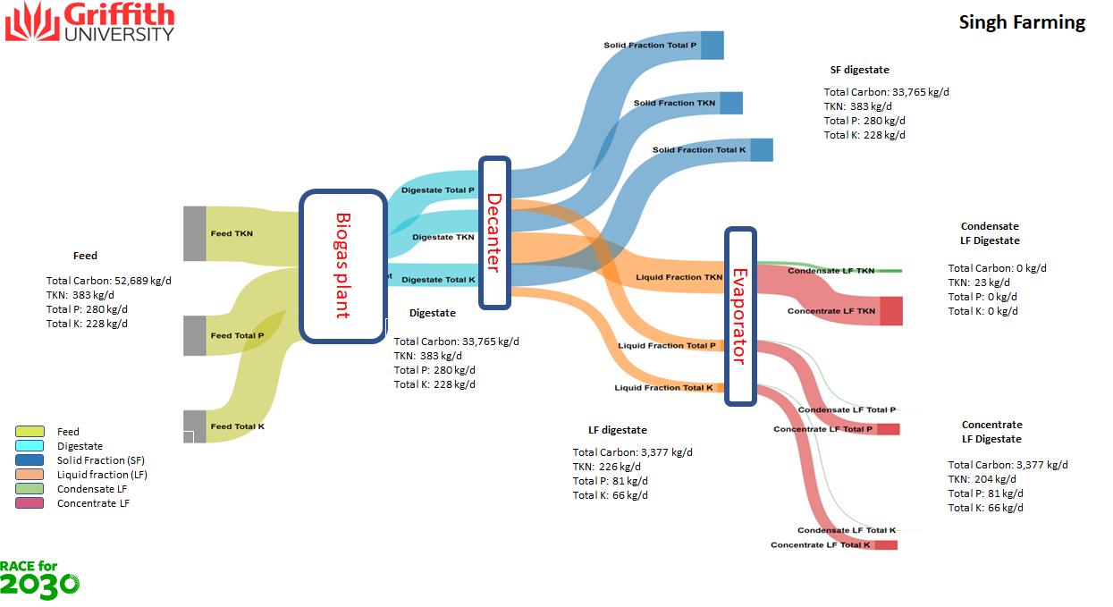
The mass balance and nutrient distribution in the whole digestate and after solid-liquid separation is presented in Table 4 and Figure 3, respectively. The whole digestate had a solids content of 6.1%. An attempt to improve the nutrient content of the digestate was made by separating the digestate into solid and liquid fractions using a decanter centrifuge. Results showed that the solid fraction with 30% solids and 74% w/w by mass accounted for 41, 71 and 71% of total Kjeldahl nitrogen (TKN), phosphorous pentoxide (P2O5) and potassium oxide (K2O) content of whole digestate, respectively. On the other hand, the liquid fraction (1.2% solids) accumulated the remaining TKN, P2O5 and K2O (see Table 4)

The nutrient content and fertiliser value of different fractions of digestate are presented in Table 5. The N, P and K fertiliser content (%) in digestate were 1:0.7:0.6. Separation of the digestate into solid and liquid fractions did not improve the fertiliser value of the fractions. Solid digestate had N:P:K values of 0.15:0.19:0.16. One option is to dry the solid fraction and sell it as soil conditioner. Based on the nutrient value, the solid fraction can be sold at $10/t. The liquid fraction (1.2% TS) with relatively low N content (0.93 g/kg FM) will be recycled as process water. An attempt was made to improve the fertiliser value of the liquid by using evaporation technology (see Table 5) Evaporation of the liquid fraction with 90% volume reduction can concentrate (27.96 t/d) the N:P:K content to 0.65:0.26:0.21 but will incur an energy requirement of 540 kWh/d. The market value for this product has been estimated to be $15.72/t. Mixing the dried solid fraction with the concentrate did not improve the overall value of the product as fertiliser and thus its market value remained low ($10.50/t). Thus, recycling of the liquid fraction as process water in the biogas plant and sale of solid digestate are the best digestate management options

1.8 Greenhouse gas emission reduction

Table 6 presents the annual greenhouse (GHG) emissions that could be avoided on adopting AD technology for generating renewable biogas and using it for heat and electricity generation (Scenario 1), BioCNG (Scenario 2) and BioRNG (Scenario 3). Total GHG emissions from fossil fuel use in the transport of 5,000 t/a of chicken manure has been estimated at 50 t/a carbon dioxide equivalence (CO2-e). Emissions from the transport of bagasse and mill mud is not included as these two feedstocks are available on site. GHG emissions from their current business-as-usual (BAU) applications vis-à-vis as feedstocks in AD process were also calculated. Diverting 30,000 t/a of mill mud from current stockpiling (BAU) to an AD pathway would avoid 29,944 t/a CO2-e. Similarly, diverting 20,000 t/a of bagasse from combustion in boilers (BAU) to an AD pathway would avoid 269 t/a CO2-e, while diverting 5,000 t/a of chicken manure from composting (BAU) would avoid 105 t/a CO2-e. Thus, the total GHG emissions avoided from current management practices of these feedstocks was estimated to be 30,318 t/a CO2-e. Renewable energy in the form of heat and electricity generation in Scenario 1 could replace 15,429 t/a CO2-e of emissions generated from equivalent heat produced from natural gas and electricity from coal, respectively. Similarly, use of biogas for BioCNG production and use in Scenario 2 could avoid 7142 t/a CO2-e emissions from natural gas. Finally, the annual emissions saved on the use of anaerobic digestate in the studied scenarios is about –354 t/a CO2-e. Overall, the net GHG emissions avoided in Scenario were 45,343 t/a CO2-e, which is 6,942 t/a CO2-e more than the values obtained for Scenarios 2 and 3

1.9 Economic analyses

For economic analyses, capital costs (CapEx), operating costs (OpEx), revenue and return on investment (ROI) along with payback period (PBP), net present value (NPV) and internal rate of return (IRR) were calculated. In addition, sensitivities to different project parameters were also calculated and compared for the three studied scenarios. The economic assessment undertaken is based on the best available data and uses a combination of internal plant and equipment cost data and literature reports adjusted for plant size. Where equipment cost data are used, the associated discipline costs for installation have been apportioned based on industry experience for the delivery of process plants within Australia. Operating costs are determined independently for each of the four main components. There remains an opportunity to integrate elements of plant operation and further reduce these costs by examining the control systems and remote monitoring and through more detailed analysis. Economic analyses were carried out for plant life of 25 years and that there is no assumed change to plant outputs over the course of its life.

Project CapEx includes the following parameters:

• project development fee

• engineering, procurement, and construction management (EPCM) 18% of CapEx

• plant equipment

• plant infrastructure (civil works, concrete works, roads, pipe work, powerlines)

• plant commissioning

• contingency 30% of total CapEx.

Project OpEx includes the following items:

• electricity to plant

• biomass ensilation

• BioRNG grid connection metering

• O&M costs

The operation and maintenance (O&M) cost estimate represent a site-based attendance for plant operation and as-required maintenance regime and is based on a percentage of the mechanical and electrical equipment as well as manpower estimates. An estimated 8% of the CapEx including contingency was considered as O&M costs. The following assumptions have been used for the financial modelling:

• Feedstock cost of $40/t of chicken manure and $25/t of sugarcane bagasse and $0/t of mill mud

• Fossil fuel electricity cost at $160/MWh to meet parasitic electrical and heating demand of the biogas plant.

• Biomass ensilation cost of $0.16/kg.

• Biomethane grid connection metering cost of $0.8/GJ.

• Biogas plant revenue was calculated at sale prices of $8.5/GJ of BioRNG to grid, $16/GJ for BioCNG and $200/t for uncompressed food-grade BioCO2

• Feed-in tariffs of $85/MWh for electricity to grid injection and sale of solid digestate at $10/t as soil conditioner.

• Liquid digestate sale is not considered due to low nutrient content.

• Australian Carbon Credit Units (ACCUs) at $30/t CO2-e and green certificates at $3/GJ were considered in the financial model. ACCUs were calculated for the total GHG emissions avoided from use of renewable energy and the associated GHG emissions (see Table 6). Green certificates were calculated for energy content in the biomethane produced.

Profitability Analysis

The profitability of the plant was assessed using four metrics:

- the return on investment (ROI)

- the payback period (PBP)

- the net present value (NPV)

- the internal rate of return (IRR)

The NPV represents the economic value of the project at present by considering the time value of money throughout the project lifetime of 25 years. A positive NPV indicates economic feasibility.

������������ = ������������ +

TCI – Total Capital Investment Cost

CFn - cash flow of the year n r – discount rate

The payback period (PBP) expresses the period which is necessary for full investment recovery.

������������ =

PNET – net yearly profit.

The IRR corresponds to the discount rate when the NPV becomes zero.

The ROI is the percentage of the investment recovered in a year of operation.

������������ = ����������������

• NPV was calculated at a discount rate of 10%

• Cash flow was scheduled at an inflation rate of 0% at the start of the project Year 1 and then NPV was calculated at a fixed net income over the project life of 25 years. About 80% of CapEx payment is scheduled in the Year 1 and the remaining 20% in Year 2.

1.9.1 Capital cost (CapEx) estimate

Table 7 and Figure 4 summarise CapEx for the three studied scenarios. The general breakdown of the individual categories of CapEx into sub-components depends on the equipment of the biogas plant’s process line with some significant and recurring categories of expenditure. Total CapEx increased from $13 million in Scenario 1, when biogas was used for 100% heat and electricity generation in CHP, to $15–16 million, when the biogas is upgraded and compressed to BioCNG (Scenario 2) or to BioRNG (Scenario 3). Investment in both CHP and biogas upgrading equipment in Scenarios 2 and 3 would incur an additional CapEx of $3–4 million. Of the total CapEx, biogas plant alone accounts for 77% in Scenario 1, 66% in Scenario 3 and 63% in Scenario 2.

Thus, the total investment required varied from a low of $20 million for Scenario 1 to $24–25 for the other two scenarios (Table 7).

1.9.2 Operating cost (OpEx) estimate

OpEx costs were calculated and are presented in Table 7 and Figure 4 O&M costs accounted for 8% of the CapEx and thus varied slightly from Scenario 1 to Scenario 3. The major operating cost is derived from the cost of the feedstock (bagasse and chicken manure import) and biomass storage with this cost representing ~37–42% of total operating costs. In Scenarios 1 and 3, O&M accounted for 58% of OpEx costs. The corresponding values for Scenario 2 was 62%.

Commissioning cost

Development fee

Balance of plant

Feed storage and feeding system

Infrastructure

Biogas collec�on and storage

Biogas reactor

Post-storage tank

Digestate processing

Pasteurisa�on

CHP

BioCO 2 recovery and liquifac�on

Biogas Upgrading Unit incl comp

1.9.3 Revenue and ROI

Earnings (earnings before interest, tax, depreciation and amortisation or EBITDA) analysis was undertaken for the project to assess aspects associated with operating cash flows. The results of this analysis are shown in Table 7 and Figure 5 The data shows that the project concept at the scale of 2.2 MW biogas plant would result in revenue of ~$3.4 million per year for Scenario 1 and $4.3 million for Scenario 3 while Scenario 2 would generate $5.3 million per year. In Scenario 1, 48% of revenue would result from the sale of electricity to the grid while the remaining revenue comes from ACCUs and sale of solid digestate

However, ACCUs are not currently available in Australia and a methodology to ascertain methane emissions from these feedstocks is required. Sale of BioCNG and BioCO2 in Scenario 2 accounted for 60% of the revenue. Internalising the environmental benefits of avoided GHG emissions through inclusion of ACCUs and green certificates, the ROIs for the studied scenarios are 4.8, 10.6 and 6.7% for Scenarios 1, 2 and 3, respectively. Conversely, ROIs without ACCUs and green certificates would be –1.9 to 4.2%. Thus, ACCUs

($30/t CO2-e) and green certificates ($3/t CO2-e) play an important role in making bioenergy projects such as this economically viable and provide confidence to investors.

1.10 Sensitivity analysis

Table 8 and Figure 6 present the results of a sensitivity analyses carried out to understand the importance of feedstock gate fees, government grants, feed-in tariffs and ACCUs in improving the revenue and thereby ROI of bioenergy projects The influence of feedstock gate fees of $0–50/t for future organic wastes (e.g food organics and garden organics (FOGO) or food wastes) showed that an increase in gate fees will increase the ROI linearly. Overall, Scenario 2 showed the best response to an increased gate fee, indicating that use of biogas for BioCNG and sale of surplus electricity will bring better economic ROI In Europe especially in Denmark and Germany, feedstock gate fees of €20–40/t have been widely used. Similarly, the influence of investment grants on ROI showed that any investment grant support <30% of the total CapEx will have only marginally increase ROI On the other hand, an investment grant support of >40% of total CapEx will have a significant impact on ROI. As expected, an increase in the feed-in tariff price for electricity from $0.085/kWh to $0.21/kWh increased the ROI linearly Similarly, ACCU prices of $30–70/t CO2-e also showed a similar trend as that of gate fees, indicating that both gate fees and ACCUs are the major economic parameters required to make these bioenergy projects economically viable.

The scale of production was calculated at four different plant sizes - 2.2 MW, 4.4 MW, 6.6 MW and 8.8 MW. CapEx was increased by 50% from 2.2 MW plant to 4.4 MW and 6.6 MW. On the other hand, OpEx increased linearly by 20% and 30% from the 2.2 MW plant size to the 4.4 and 6.6 MW plants, respectively For the 8.8 MW plant size, CapEx increased by 100% while OpEx increased by 40% than the 2.2 MW plant.

Notes 1 DR: discount rate electricity price

Overall, scale of production has a more profound influence on the ROI and production costs of electricity, BioCNG and BioRNG than any of the parameters studied (Figure 7 and Table 8). When increasing the plant design capacity from 2.2 to 8.8 MW, the cost of electricity production drops sharply when the plant size is increased from 2.2 to 4.4 MW and then drops more steadily as the plant size is increased from 4.4 to 8.8 MW. At the same time, the ROI increases significantly when the plant size is increased from 2.2 to 6.6 MW and flattens thereafter Both these results suggest that a large-scale centralised biogas plants with an average plant size of about 6.6 MW and digesting 450 t/d of feedstock would be economically viable in Australia with a ROI of 27–33%.

1 and

1 (CHP + electricity), Scenario 2 (CHP + BioCNG) and Scenario 3 (CHP + BioRNG). Please note that Scenarios 2 and 3 use biogas for BioCNG and BioRNG production, rather than electricity production, so are not present on the electricity price figure as they do not export electricity return on investment (ROI)

Figure 7. The influence of plant capacity on return on investment (ROI, %) and cost of electricity ($/MW), BioCNG ($/GJ) and BioRNG ($/GJ) for Scenario 1 (CHP + electricity), Scenario 2 (CHP + BioCNG) and Scenario 3 (CHP + BioRNG). Please note that the values for costs in Scenarios 2 and 3 are identical, so Scenario 2 is also represented by the red dots.

The cost of production of electricity (in $/kWh) or biomethane (in $/GJ) is presented in Figure 7. The cost of production of electricity decreased from $0.11/kWh at a 2.2 MW plant size to $0.04/kWh when the plant size reached 8.8 MW. Similarly, the estimated cost of biogas upgrading and feeding biomethane into the natural gas grid decreased from $19.71/GJ at 735 m3/h of raw biogas upgrading capacity to $6.9/GJ when the upgrading capacity is 2940 m3/h raw biogas. For BioCNG production, the cost of production decreased with an increase in upgrading capacity from $19.56/GJ (750 m3/h raw biogas) to $6.84/GJ (3000 m3/h raw biogas).

1.11 Conclusion

The study shows that a 2.2 MW biogas plant can generate approximately 9.35 million Nm3 of biogas per year through codigestion of 20,000 t/year of sugarcane bagasse and 30,000 t/year of mill mud with 5,000 t/year of locally available chicken manure. Nonetheless, it is necessary to further improve the energy and product efficiency to make the biogas plant economically viable. Financial analyses show that the total investment required for the biogas plant could vary from $20.43 to 24.95 million and depends on the technology and equipment used for biogas use. However, the ROI depends on the revenues generated especially from variable parameters such as feedstock gate fees, government investment grants and guaranteed feed-in tariffs, ACCUs and green certificates. Internalising the environmental benefits of avoided GHG emissions through inclusion of ACCUs and green certificates, the ROIs for the studied scenarios are 4.8, 10.5 and 6.7% for Scenarios 1, 2 and 3, respectively. Conversely, ROIs without ACCUs and green certificates would be –1.9 to 4.2%. Sensitivity analyses showed that an AD plant of 6.6 MW capacity will significantly reduce costs and become among the most competitive technologies in renewable energy and carbon markets with ROIs of 27–33%. Thus, onsite production and/or use of renewable energy will enable farmers to achieve sustainable management of agricultural wastes and help to decarbonise the agricultural sector.

Far Northern Milling, owners of Mossman Sugar Mill, have selected Helmont Energy as the proponent of their AD project, and plan to achieve practical project completion by 2024.