Queenwood acknowledges the Cammeraigal people who are the traditional custodians of the land on which the School is built and we pay respect to Elders past, present and emerging.
DR
CAMILLA HOYOS Q1998
B.APPSC (CONSUMER SCIENCE), B.SC (HONS), MPH, PHD
What I love about being a scientist is that I get to ask and answer questions that will potentially go on to help people. Science is all about discovery and the great thing is that there are so many areas that still need investigating. New discoveries can affect our lives in so many ways. This includes advancing new scientific knowledge that allows us to create new technology, address societal issues, solve everyday problems, and help to inform the decision makers of our community. What drew me to Science was the critical thinking and problem solving it involved. I liked having a question to answer and learning how to answer it. My journey into Science would have not happened without the amazing experience I had at Queenwood and the teachers that made lessons very enjoyable. I was also interested in
Queenwood Alumnus and CSIRO STEM Collaborator in schools Dr Camilla Hoyos reflects on the value of studying Science in society.
research from a young age, which grew during my university degree. Even though I had done a Science degree, I had focused more on health and had not completed labbased courses. I decided I wanted to do an honours project where I worked researchers and benefitted greatly from my experiences in a public health unit. After graduating I started looking for jobs in clinical research and my first job involved working with people living with asthma. I loved my job and where I worked, so much so I still work at the same medical research institute 21 years later. I learned new techniques such as lung function testing and met new people every day. Very quickly, however, I found that I wanted to learn more so I could identify the questions that needed to be answered and then design the studies to answer them. I chose to do a Master of Public Health and then a few years later a PhD in sleep medicine, the area in which I still work today.
One of the great things about being a researcher is new opportunities, some of them rather unexpected. A few years ago, I decided to volunteer for the CSIRO STEM professionals in schools’ program which matches scientists of all kinds with different schools. To my delight an opportunity to partner with Queenwood arose. In 2018/19 I was involved in the Researchers Initiative where the students were able to develop their own research question and study. We also had a visit to the Woolcock Institute where students visited the sleep lab and did activities such as driving simulation and learning how we measure sleep. It is these experiences that become prominent highlights of my work. Engaging with the community and particularly young people who will go on to be the next generation of researchers, answering difficult questions and making amazing, life-changing discoveries is one of the most enjoyable elements of my job! •
DR MICHELLE GLEESON HEAD OF SCIENCE
B.SC (BIOTECH), B.SC (HONS), PHD, GRAD DIP ED
I am delighted to introduce the Queenwood Journal of Science Extension, Volume 2, 2024. Science Extension is a multidisciplinary one-unit course studied by Year 12 students in addition to one or more of the Biology, Chemistry and Physics courses in Stage 6.
Science Extension was first taught in NSW in 2019 and is unique in being the only course to culminate in a 2 hour online examination. In addition to the exam, students design and conduct an individual research project and prepare a Scientific Research Report. A selection of these reports, somewhat like an Honours thesis in miniature, are showcased here to demonstrate the depth of their talent, initiative and perseverance.
So, why should students study Science Extension? It is a unique opportunity for students
Our Head of Science, Dr Michelle Gleeson introduces the Science Extension program at Queenwood.
to branch out into an area of passion or interest beyond the constraints of the curriculum. The course is less about content and knowledge, than the processes of working scientifically. Via the course, students move from studying science to experiencing what it means to becoming a scientist themselves. The tangible benefits include substantial gains in critical thinking and analytical skills, which are transferrable to their other courses and onwards into their future studies. The next generation of scientists have a massive job on their hands. They will need to devise innovative solutions for problems we do not even know about yet, to support a growing world population existing in a dynamic and deteriorating environment. There is a reason why Science Extension students are being courted by top universities through their mentoring programs, as they are ready to hit the ground running and thrive in the tertiary Science environment.
2024 marked the sixth year of running Science Extension at Queenwood, a vibrant and richly collaborative environment facilitated by two teachers. The cohesive nature of the class environment is key to its success. Thrill and disappointment, resilience and determination each come to the fore when students work on their individual projects during this course and we would like to congratulate them on their outstanding performances. These Scientific Research Reports are a fitting tribute to the tenacity, tears, and ultimately the triumph of accomplishment.
We hope you enjoy exploring their work, and we are sure you will agree that our future is in great hands. We look forward to seeing where this experience leads them. •
MS MERRILYN LEAN SCIENCE EXTENSION TEACHER B.SC DIP ED
Science is a unique process that involves asking questions, making observations, thinking creatively and critically, and testing hypotheses based on the scientific method. This is the core of the practice of Science. Science Extension is a course that I love to teach as it allows students to deeply explore a research question of their choosing in a way that is not possible in other subjects. I have been teaching for a long time, both the HSC and IB, in more than one state in Australia, and this course is unique as it provides students with the opportunity to think like a scientist, and not think just about Science. Analysing evidence-based research increases the ability of the students to identify the intent and thus validity of the vast amounts of information that they encounter in mass media, generating more discerning viewpoints through
Science Extension Teacher Ms Merrilyn Lean, discusses the unique process involved in the subject.
their questioning. Science Extension is a course unlike any other in the HSC. Discussions, exploration of scientific papers, and model development and analysis provide opportunities for students to learn from each other and explore their varying opinions to identify what makes them reason differently and ultimately make the decisions that they do. It is a joy to be a part of learning experiences that open the eyes of students as they progress through the course, starting with content that they are very familiar with like bias, and ending with ideas that are highly complex and that are fundamental to the history of philosophy and thus science, such as rationalism and empiricism. I love the passion and confidence that the students demonstrate as their ability to explore their own ideas scientifically grows, and when they recognise that they are now experts in whatever subject they have chosen to investigate. I love
being a part of the development of the critical thinking and problemsolving skills of the students, as they gain more experience in manipulating technological equipment and data bases, confidently taking the lead on their own projects. It is highly rewarding seeing the students give so much of themselves, gaining insights into their own strengths and weaknesses. This course prepares students for the experiences that they will encounter in their future studies at University.
There is a great sense of achievement and pride amongst the students when they finally submit their work and it is a great pleasure to present these Scientific Research Reports. •
Introduction Jessica Mulcahy Q2023
JESSICA MULCAHY
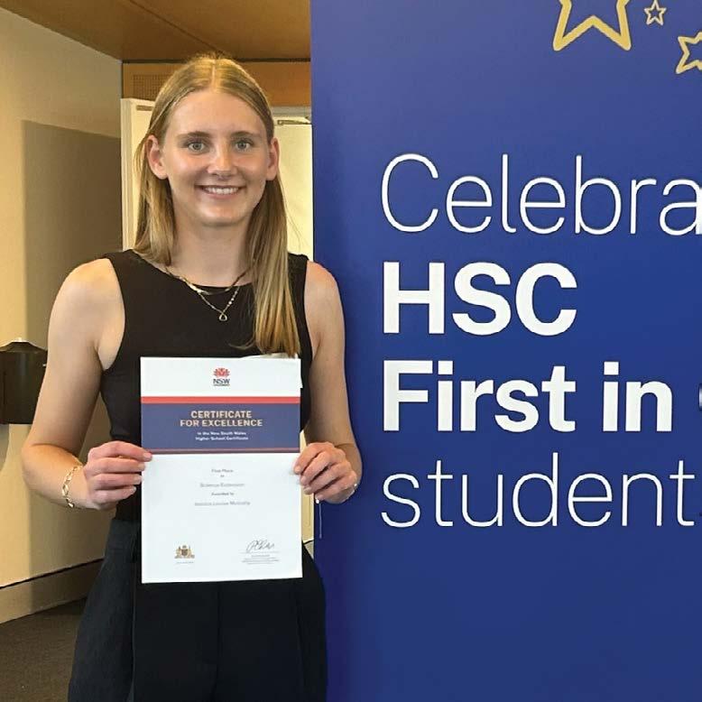
Q2023 FIRST IN STATE SCIENCE EXTENSION
From starting off in 2024 enrolled in a Medical Studies degree at Sydney University to a couple of months later moving to the Gold Coast after getting into Medicine at Bond University, what I have learnt in Science Extension has continuously helped me throughout the last two years. The Science Extension course equipped me with the necessary skills to meet the challenges of a university degree and the ability to balance the work within my course. The Science Extension course involved research of my own scientific project, as well as data analysis. This background knowledge of how to interpret data has helped me in the statistics topics within my course, as well as my understanding of research papers when writing assignments. On another level, the more self-directed nature of parts of the course allowed me to
Jessica Mulcahy reflects on her Science Extension experience as a student at Queenwood.
continue to build independence in Year 12, which is essential in university, which requires much self-motivation. I found Science Extension helped build confidence in my ability to manage my workload, and it has increased my ability to understand new and difficult concepts.
Since leaving school, I have been able to reflect upon my time at Queenwood and have come to realise the importance of giving everything a go. Whilst doing extension subjects can seem daunting, choosing Science Extension was one of the most beneficial and rewarding choices I have made, where the course allowed me to further my interest in science and research many new things. Science Extension is definitely a course I would recommend, as you never know where it may lead you! •
To investigate an alternative method to determine the glucose content and therefore glycaemic index of different types of rice.
JESSICA MULCAHY Q2023
Abstract
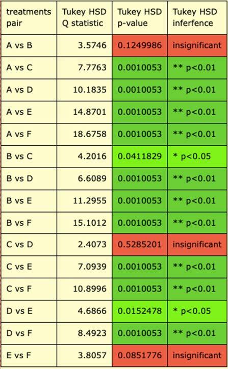
The purpose of this study is to determine an alternate method to investigate differences in the glucose concentration of different types of rice. Globally, rice provides 35-60% of the caloric intake of over 3 billion people’s diet; however, there is a lack of knowledge about the glucose content of the varieties. A spectrophotometric analysis measured the glucose content of brown, white, brown basmati, white basmati, jasmine and risotto rice at a wavelength of 740λ . An ANOVA found a significant difference (p = 3.4688 × 10 -6) between the glucose concentrations of the 6 types of rice. The Tukey HSD test found the differences between the following types of rice to be significantly different: jasmine and brown basmati, jasmine and white, jasmine and risotto, jasmine and brown, white basmati and white, white basmati and brown, brown basmati and brown, white and brown. Brown rice had the lowest average glucose concentration, followed by risotto rice, both brown basmati and white rice, white basmati rice and jasmine rice. The results from this study can inform decisions about the type of rice eaten to prevent and manage type 2 diabetes, as there is a causal link between the Glycaemic Index (GI) of foods and type 2 diabetes. Diets with high GI foods predispose people to higher blood glucose levels, increasing their risk of developing the disease.
1. Literature review
Glucose is a monosaccharide that is critical to essential metabolic processes including respiration. When glucose enters the bloodstream, it serves as the primary source of energy for the body, and excess glucose is stored in the liver and muscles as glycogen (Goyal, 2022).
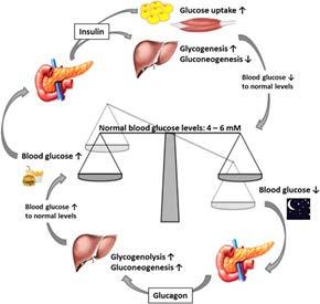
As seen in Figure 1, to maintain stable blood glucose levels, the body relies on the coordination of two hormones: insulin and glucagon. Insulin is produced by beta cells in the pancreas and increases in response to elevated blood glucose levels. Its main function is to promote glucose uptake by liver and muscle cells, converting it into glycogen for storage, while also facilitating the uptake of glucose by other body cells. Conversely, if the blood glucose level is too low, the alpha cells in the pancreas are stimulated to produce glucagon which breaks glycogen in the liver into glucose to release it into the blood (Miller et al, 1997). Simultaneously, a drop in glucose will cause a decrease in insulin and inhibitive signalling to alpha cells, thereby producing more glucagon and triggering the efflux of glucose from cells via breakdown of glycogen. This action helps regulate blood glucose levels and maintain homeostasis (Goyal, 2022).
Glucose is a component of complex carbohydrates including polysaccharides and glucosides, and consequently, holds significant importance in food products (Roder, 2016). The determination of glucose content as well as other nutrients such as vitamins enables a precise evaluation of the nutritional composition, and thus potential health impacts of food. The monitoring of sugar intake is particularly pertinent to type 2 diabetes as it is necessary for people to control the levels of glucose substantially via diet in their blood. Diabetes is a non-infectious disease that occurs when glucose level is constantly too high in the bloodstream, above tolerance levels of 3.5-8mmol/L (Omar, 2018). The disease affects 9.3% of the global adult population aged between 20 to 79 years (World Health Organisation, 2023). There are two types of diabetes, which differ based on their disease mechanism.
Type 1 diabetes is an autoimmune condition where the body’s immune system destroys the beta cells in the pancreas that are responsible for the production of insulin (Smith, 2023). The cause of this autoimmune disease is not comprehensively understood, although many believe that it is linked to a Coxsackie virus B infection in which shared antigens contribute to the development of an autoimmune response (Zafer, 2019). There is currently no cure for type 1 diabetes, but it can be managed through monitoring of glucose levels and use of insulin injections (Smith, 2023). In type 2 diabetes the body becomes resistant to the effects of insulin. In early stages of the disease, insulin levels are very high as the beta cells increase production of the hormone to attempt to overcome the high amount of resistance. Subsequently beta cells become overworked and damaged, losing the capacity to produce enough insulin. The disease can result from an unhealthy diet, weight gain and a lack of exercise, and many people need oral medications and insulin injections to manage the disease (Goyal, 2022). Type 2 diabetes accounts for approximately 8590% of all diabetes cases and is growing in prevalence (World Health Organisation, 2023). Over time, type 2 diabetes can lead to heart, blood vessel, kidney, nerve, and eye damage due to the high glucose levels leading to advanced glycation end-products where there is an interference with the blood supply to tissues, resulting
in systemic inflammation. This inflammation reduces the elasticity of blood vessels as it interferes with the production of nitric oxide (NO) in the endothelial cells of the blood vessel walls, leaving people prone to atherosclerosis (Smith, 2023).
The Glycaemic Index (GI) of individual foods is one way of classifying types of food. It grades food on a scale from 0 to 100 based on the rate at which the food is digested and the resultant increase in the blood glucose levels, usually over a period of two hours (LeWine, 2021). Glucose has a GI value of 100, and other foods are then compared against this rate, where a low GI value is between 1-55 and includes foods such as green vegetables and eggs. A medium GI value is between 56-69 and includes foods such as raisins and multigrain bread and a high GI value is 70+ and includes foods such as white rice and potatoes (LeWine, 2021). The GI of foods is impacted by many different factors such as the type of starch and sugar present, acidity, and the ripeness of the food (Ellis, 2019).
The Glycaemic Index is directly related to type 2 diabetes, as foods with higher GI will increase the blood glucose levels at a faster rate (Ellis, 2019). Higher GI foods can make it harder to control type 2 diabetes as they are rapidly digested which results in larger spikes in blood glucose. Beta cells will have to work particularly hard with a constant large intake of high GI foods, which can result in insulin resistance. For people who have been diagnosed with type 2 diabetes, lowering their intake of high glycaemic index foods can help control and maintain a stable blood glucose level (Endocrine Society, 2022). This information is also important for people without types 2 diabetes as it can assist in weight loss, and as a preventative measure for the disease.
Rice is a food staple for over 3 million people throughout the world and knowledge of the differences in the types of rice is extremely important in planning meals, to reduce glucose intake (World Health Organisation, 2023). Rice with lower GI include brown rice (GI 55), risotto rice (GI 58) and brown basmati rice (58). Rice with higher GI include jasmine rice (GI 68), white basmati rice (GI 65), white rice (GI 72) (Sydney University, 2020). The glycaemic index of a food is determined by measuring the incremental
area underneath a blood glucose curve of a person over the duration of two hours after a meal. This is a complex method to determine a singular number, and this study will aim to investigate an alternate method to determine the glucose concentration in rice. In addition, there is a lack of conclusive evidence from the limited studies within this area and hence further research is required to be undertaken to directly compare these six different types of rice. This information is essential as it can assist governments and organisations develop education programs and campaigns to educate the public about the differences in glucose within types of rice, with the aim of preventing type 2 diabetes. This study will seek to fill the gaps in this area to determine whether this alternate method is an appropriate measure of glucose concentration within different types of rice which correlates with the glycaemic index. Due to the effects from type 2 diabetes, it is necessary for further research to be conducted into an alternate method to the current complex method of determining the glycaemic index to determine the availability of glucose levels in different foods, to make people aware of how they could alter their diet to reduce the risk of developing the disease.
2. Scientific research question
To evaluate an alternate method of determining the glycaemic index of different types of rice.
3. Scientific hypothesis
The glucose concentration of rice varieties, as measured by the spectrophotometric analysis, will correlate with the glycaemic index scale.
Jessica Mulcahy
FIGURE 1: Glucose homeostasis (Roder, 2016)
4.1 Risk/ethical assessment
Risk Amelioration
Glass beakers dropping on the floor and smashing, where glass could cut a person’s skin causing lacerations.
If water is spilt on the ground, a person could slip on it and fall over, causing bruising or head injuries.
Ensure to keep the beakers away from the edge of the desk, and immediately clean up any broken glass.
Keep beakers with water away from the edge of the desk and if any water is spilt, immediately clean it up.
8. Data was graphed for the standard curve. 4. Methodology
Getting a finger caught or stuck in the centrifuge whilst it is spinning the supernatant.
Keep hands far away from the centrifuge whilst it is operating and ensure it has been completely turned off before retrieving the supernatant solutions.
Ethical considerations: Within this investigation, there is no use of animals or humans within the testing of glucose concentrations which meant there were minimal ethical considerations. However, a reduction of resources for the food materials used was considered to ensure that excess materials were not wasted during the investigation.
4.2 Justification of equipment
Within the experiment a centrifuge will be utilised, to ensure the solution will be spun at a sufficient rate to separate the heterogenous mixture into the supernatant and solid components. The spectrophotometer is able to read absorbance to three decimal places, ensuring accurate readings, which is also the case for the mass balance. The micropipette has 0.5 ų L increments, with an uncertainty of ±0.25 ų L, further ensuring accurate data is collected.
4.3 Complications of experimental process
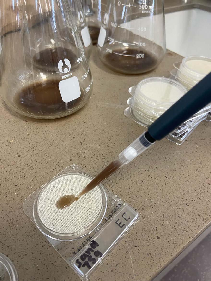
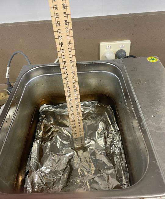
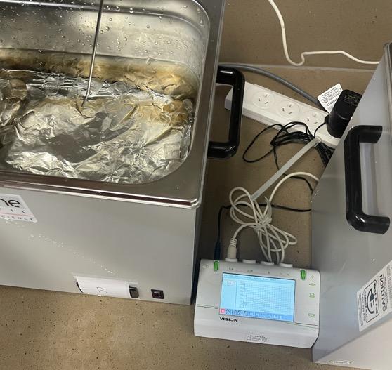
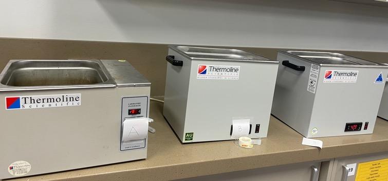
Within this investigation, data was successfully collected for the standard curve, measuring the absorbance of different concentrations of glucose. When determining the absorbance of the six different types of rice, the first method as stated below in section 4.4 was attempted to be followed; however, in addition the supernatant solution of rice, starch, amylase and Benedict’s solution was heated prior to the solution being spun in the centrifuge which was not successful after over a month of manipulating the method and trialling different equipment. The method was then revised to what is described in section 4.5, however, after numerous trials this method was also unsuccessful. Therefore, by using the standard curve as well as published information about the Glycaemic Index levels of different types of rice (Sydney University, 2020), data was extrapolated to create an estimated data set for the research project, suitable for further analysis in the absence of experimentally derived data.
4.4 Method for creating the standard curve
1. 1mL of Benedicts solution and 0.5mL of water were collected using a micropipette and added into a 1.5mL Eppendorf tube and mixed well to ensure sufficient integration.
2. Step 1 was repeated 7 times but the 0.5mL of water was replaced with 0.5mL of 5%, 10%, 15%, 20%, 25%, 30% and 35% glucose solutions.
3. The eight Eppendorf tubes were spun down for 5 minutes in the centrifuge.
4. After 5 minutes, for each concentration of glucose, 0.5mL of the supernatant was placed in a cuvette using a micropipette.
5. 2.5mL of water was added to each of the 8 cuvettes and mixed well.
6. The first cuvette with distilled water was placed into the spectrometer, where the absorbance value was read at the wavelength at 740λ from the computer which is suitable due to the reagent of Benedicts solution being used.
7. Step 6 was repeated 7 more times with the remaining concentrations of glucose, where all absorbance values were recorded.
4.5 Method for measuring the absorbance of rice solutions
1. 2g of brown rice was measured using a mass balance and blended in a blender until in the form of a powder.
2. The rice was further ground into smaller fragments with minimal grains present using a mortar and pestle.
3. 100mg of brown rice was poured into a 1.5mL Eppendorf tube using a small funnel.
4. 5mL of a 1% starch solution was measured using a micropipette and poured into the 1.5mL Eppendorf tube with the rice and mixed well.
5. 0.5mL of a 1% amylase solution was collected using a micropipette and added into the same Eppendorf tube.
6. The Eppendorf tube was left upright for 10 minutes.
7. 0.5mL of the supernatant from the Eppendorf tube and 1mL of Benedicts solution were collected, added into a small Eppendorf tube and mixed together.
8. The Eppendorf was placed in the centrifuge and spun for 5 minutes.
9. 0.5mL of this supernatant and 2.5mL of water was measured and placed into a clean cuvette.
10. The cuvette was placed into the spectrometer, and the absorbance value was read at the wavelength of 740λ from the computer.
11. Steps 3-11 were repeated 4 more times for brown rice.
12. Steps 1-12 were repeated with the different rice types of risotto, white, brown basmati, white basmati and jasmine rice.
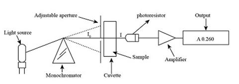
FIGURE 2: The functioning of a spectrophotometer (Trumbo et al., 2013)
5.1 Graph and table of standard curve:
Absorbance readings at 740λ based on percentage glucose
glucose (%) Absorbance (Au)
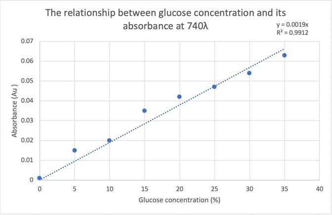
The overall trend in Table 2 and Figure 3 is that as the glucose concentration of a solution increases, the absorbance also increases, highlighted by the very high correlation as the R2 value is 0.9912. The R2 value indicates a positive relationship and a very high correlation between the glucose concentration and absorbance. The equation of the line is y = 0.0019x, which will then be used to determine the glucose concentration of solutions of rice.
*Refer to the appendix for the raw data.
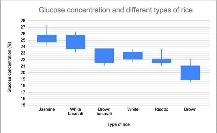
Figure 4 shows the variation in glucose concentration in different types of rice, where brown rice has the lowest concentration and jasmine rice has the highest. The glucose concentration was calculated using the equation of the standard curve y = 0.0019x where each absorbance value was substituted into the y value. The equation was then rearranged to get x as the subject to determine the glucose concentration for each rice.
Sample calculation:
Jasmine rice absorbance = 0.047 Au
y = 0.0019x where y = 0.047 Au
x = 0.047/0.0019 x 100
x = 24.737%
The types of rice with the highest absorbance were jasmine rice which had an average absorbance of 0.048 and white basmati rice which had an average absorbance of 0.046 and their glucose concentrations were 25.474% and 24.737% respectively when digested with enzyme. Both brown basmati rice and white rice had an average absorbance of 0.043 and average glucose concentration of 22.632%. Risotto rice had an average absorbance of 0.041 and average glucose concentration of 22.061%, and brown rice had the lowest average absorbance of 0.038 and average glucose concentration of 20.116%.
5.2 Graph of difference in the glucose concentration of rice
Jessica Mulcahy
TABLE 1: Spectrophotometer readings at 740 λ based on percentage glucose
FIGURE 4: Glucose concentration of different types of rice (p = 3.4688 x 10 -6).
FIGURE 3: Standard Curve of spectrophotometer readings based on percentage glucose.
5.3 Statistical analysis
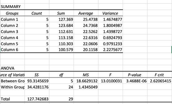
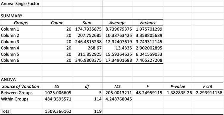
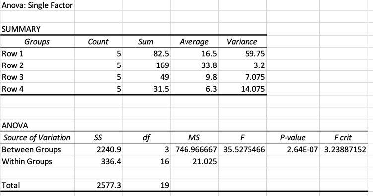
An ANOVA test was conducted as there was one independent variable where the means of more than 2 groups was being compared. The assumptions for an ANOVA test were met including data is quantitative, randomly sampled, data has normal distribution, the variation in each group is similar, means for more than two groups, replicates and not repeats and the investigation is falsifiable. The ANOVA test was conducted on Excel and the p value was determined to be 3.4688 × 10 -6 which is less than 0.05 meaning there is a statistical difference between the glucose concentration in the six groups and therefore the alternate hypothesis is to be accepted. All the assumptions for an ANOVA test were satisfied such as a large sample size, the data is quantitative, randomly sampled, the variances in each group was similar as shown in Figure 5, means for more than two groups were calculated and the investigation was falsifiable.
Jasmine and Brown basmati
Jasmine and White
Jasmine and Risotto
Jasmine and Brown
White basmati and White
0.0080463
0.0111964
0.0018067
0.0010053
0.0186683
White basmati and Brown 0.0010053
Brown basmati and Brown 0.0411424
White and Brown 0.0302201
6. Discussion
6.1 Comparison of types of rice and errors in results
The data recorded supported the hypothesis and identified jasmine and white basmati rice with the highest average glucose concentrations of 25.474% and 24.737%, which also directly correlate with the fact that both these types of rice are high glycaemic (GI) foods with GI indexes of 68 and 65. In the middle of the range, brown basmati rice and white rice had slightly lower average glucose concentrations of 22.632%. Brown basmati rice has a GI of 58, which is lower than jasmine and white basmati rice, corresponding with the decrease in glucose concentration. Risotto and brown rice had the lowest average glucose concentrations of 22.061% and 20.116% respectively. Risotto rice has a GI of around 58 and brown rice has a GI of 55, which both correlate with the decrease in absorbance and glucose concentration. However, white rice is a rice with a GI of 72 and is considered a high glycaemic index food with higher levels of glucose in comparison to the other rices tested (Sydney University, 2020). The results recorded the glucose concentration as 22.632%, which is a possible inconsistency in the results, and further repeats would need to be conducted to determine whether this is the pattern for other repeats, or other finding are recorded.
6.2 Recommendations of types
of rice
The type of rice that should be recommended to prevent type 2 diabetes are those with a lower glucose concentration, which based on the results from this study are brown and risotto rice. This is because the sugar within these foods will be absorbed into the bloodstream at a slower rate, resulting in a smaller rise in blood glucose (Zafer, 2019). Additionally, brown rice and risotto rice would be beneficial for people with type 2 diabetes as it will help them maintain a steady blood glucose level and reduce the effect of postprandial hyperglycaemia. People who have been diagnosed with type 2 diabetes or at a greater risk of developing the disease due to genetic or family history should seek to avoid consuming jasmine rice and white basmati rice due to their high glucose concentrations
which if consumed too often or in high portions will result in sudden increases in the blood glucose levels, where the beta cells will have to work at high rates to produce insulin in order to counteract the effects (Omar, 2018). Therefore, an understanding of the glucose concentrations of different types of rice can assist people in finding alternates to higher GI rice types such as jasmine rice and replace it with lower GI rice for example brown rice.
6.3 Suitability of alternate method
The method that was conducted throughout the investigation proved to be a simpler variation to how the Glycaemic Index of foods is usually determined which involves measuring the incremental area underneath a blood sugar curve of an individual person over two hours after a meal, which is a very complex process. With more time and additional resources, this simpler and less time-consuming method could be effectively implemented within laboratories to determine the glucose concentrations of different foods which correlate with their known GI. The method discussed in sections 4.4 and 4.5 was used in a study looking into ‘Quantification of Reducing Sugars Based on the Qualitative Technique of Benedict’ (Hernández-López et al., 2020), however this method focussed on looking into the differences in carbohydrates in different types of sugars. The method in sections 4.4 and 4.5 is essential in determining whether the process would be successful when analysing rice, as rice is a staple food throughout the world, where minimal changes in someone’s diet can lead to a reduction in the incidence of cases of type 2 diabetes. The method discussed was more effective than the other techniques attempted such as using a glucose meter, glucose strips, and heating the Benedict’s reagent as quantitative data is able to be collected allowing for a statistical test to be conducted. Although further experimentation needs to be conducted into the specificities and equipment requirements for this method, the outcomes of this investigation were ultimately able to answer the scientific research question and identified the potential effectiveness of this technique.
FIGURE 5: ANOVA test table which shows the level of statistical significance between the means of the different types of rice.
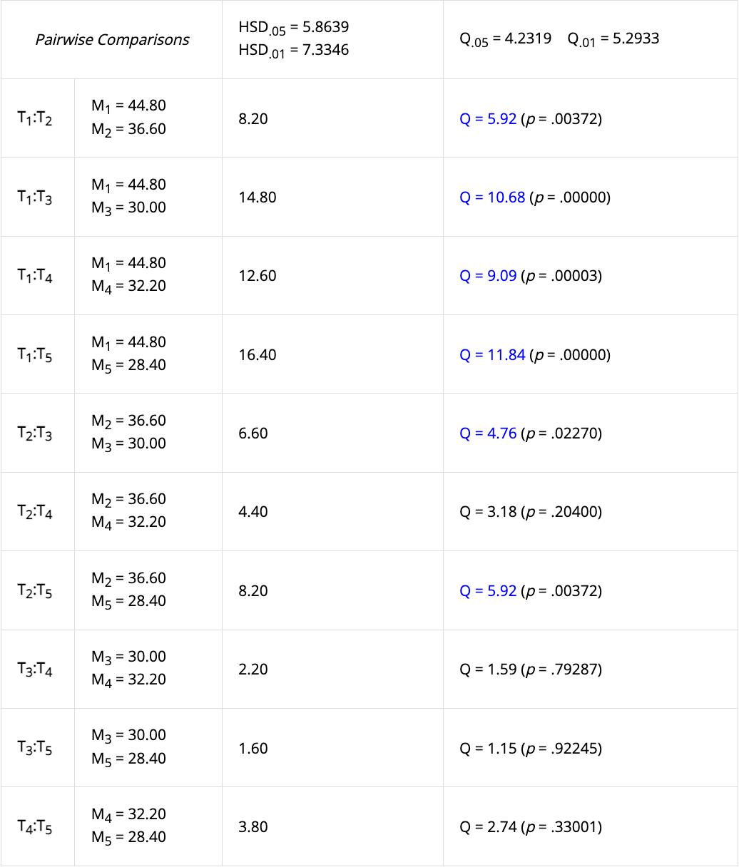
TABLE 2: Tukey HSD test which shows what types of rice are significantly different to one another.
6.4 Other studies investigating the Glycaemic Index
Studies have been undertaken to determine the link between the glycaemic index (GI) and the risk of developing type 2 diabetes in both women and men. The Nurses’ Health study uses epidemiology to analyse a variety of factors including hormones, nutrition and disease development. A 61-item food frequency questionnaire was completed by 84 360 women in 1980 to assess the link between nutrient intake and the risk of diabetes. This was followed by an evaluation of each woman’s glycaemic load which linked 915 type 2 diabetes diagnosis with their diet (Liu et al., 2002). The results from this study showed that women in the highest quartile of glycaemic load had a 40% increased risk of developing type 2 diabetes in comparison to women in the lowest quartile. In addition, the study found that cereal fiber was inversely related to the disease risk, where women with a low cereal fibre intake and high glycaemic load had a 2.5-fold higher risk of developing type 2 diabetes. The study found that women in the top quartile of whole-grain consumption had a 27% lower risk of developing diabetes, with a relative risk of 0.73 (p < 0.0001) (Liu et al., 2002).
The Health Professional’s Follow-Up Study is another Harvard based study which evaluates aspects of men’s health and the incidence of diseases. The results were similar for men who were studied as part of this study where it was found that the relative risk for developing type 2 diabetes was 2.17 for men in the highest quartile of glycaemic index and low cereal fibre intake (Liu et al., 2002). These two respective studies highlight the link between the glycaemic index and a person’s risk of developing type 2 diabetes.
6.5 Validity, reliability and accuracy of data
Repeats were conducted for this study, which allowed for an average to be calculated, minimising the chance of random errors; however, other factors such as time and equipment constraints meant consistent data was not able to be collected. Due to technical and time issues, the data for the standard curve was only able to be measured for one repeat, meaning this data recorded was not reliable as more repeats were needed to ensure the results are similar and there are no outliers.
The experiment was accurate as all the measuring equipment used had small increment values, ensuring precise data was gathered. For example, to measure the volume of various liquids, a micropipette was used which accurately measures 0.5 ų L, with an uncertainty of ±0.25 ų L, and the spectrophotometer read absorbance values to 3 decimal places. However, although the mass balance measured values to 3 decimal places, it was often hard to measure the exact mass on the mass balance of the rice as it was a small value of 2g, which could have resulted in some measurements having slightly different values in comparison to the true value. The apparatus used within the experiment was effective in measuring specific masses and volumes, although, with each of these equipment pieces, there were uncertainties that doing more repeats cannot eliminate. The investigation was valid as only the independent variable was changed which was the type of rice, whilst the dependent variable was measured which was the absorbance of the rice, and variables such as the same centrifuge and same volume of supernatant were controlled throughout the process. However, there were other variables that were harder to control, for example in Method 2 for Step 6 when needing to leave the Eppendorf tube upright for exactly 5 minutes for all rice types, it was hard to leave them for exactly 5 minutes as all the timers were started at different times. This resulted in some Eppendorf tube solutions being left for slightly longer than others, which could have impacted the separation of the mixtures and the overall glucose concentration of the rice solution. However, during the investigation, it was difficult to make the method work as the centrifuge was not able to spin the solution of rice, starch, amylase and Benedict’s solution at a fast enough rate to separate the heterogenous mixture into two components. Ultimately, this resulted in inconsistent results in the absorbance values between different types of rice.
6.6 Limitations and improvements
of study
A key limitation of the investigation is that due to the availability of equipment in the school laboratory, the method was not able to yield consistent results. Throughout the experimental process, numerous
variations of the method were trialled such as using a glucose meter, glucose strips, and heating the Benedict’s reagent before attempting to determine its absorbance. The limitations to do with the equipment available meant no method was able to yield consistent and meaningful results. Accessing the required equipment such as a larger centrifuge that is able to spin the Eppendorf tubes at a faster rate, would determine whether this is a suitable alternate method to measure the glucose concentration within foods. The results were extrapolated by utilising the limited results collected, research on the different GI indexes of rice as well as Excel to create a suitable data set to be analysed.
6.7 Future directions of scientific research
Currently, there has been minimal large-scale investigations into determining the differences in the glucose concentration of different types of rice and how this directly links to type 2 diabetes. Therefore, a future direction of scientific research could be to investigate further the significance of this link with the aim of informing governments and agencies to promote healthy eating. Education programmes and campaigns could be developed by governments to spread information about the type that should be incorporating into the diet of those at risk of type 2 diabetes. In the long term this would have numerous benefits on society as it can act as a prevention method to aim to reduce the incidence of type 2 diabetes.
7. Conclusion
This alternate method for measuring glucose concentration in different types of rice is a simpler variation to how the glycaemic index of foods is usually determined, which can be further implemented by laboratories. All types of rice had differences in their absorbance which correlated to different glucose concentrations. The order of rices from the highest to lowest glucose concentration was jasmine, white basmati, white, brown basmati, risotto and brown rice. The results recorded using the alternate method showed a correlation between glucose concentrations and the known glycaemic index rating of the different types of rice, highlighting the suitability of this method. The information collected within this investigation is applicable to wider society where people are aiming to decrease or monitor the amount of glucose they are consuming. They should mainly eat brown and risotto rice which have lower glucose concentrations and ultimately have a decreased effect on the blood glucose levels. However, advanced research is required to do with this area to investigate the suitability of the process as an alternate method to determine the glucose concentrations of different types of rice which correlate with their known glycaemic indexes. •
Jessica Mulcahy
8. References
Ellis, E. (2019). What is glycaemic index. https:// www.eatright.org/health/wellness/diet-trends/ what-is-glycemic-index
Goyal, R. (2022). Type 2 Diabetes. https://www. ncbi.nlm.nih.gov/books/NBK513253/ Hernández-López, A., Felix, D., Sierra, Z., Bravo, I., Dinkova, T., & Avila-Alejandre, A. (2020). Quantification of Reducing Sugars Based on the Qualitative Technique of Benedict. Retrieved from https://www.ncbi.nlm.nih.gov/ pmc/articles/PMC7758970/#!po=28.0488
LeWine, H. (2021). Glycaemic index for 60+ foods. https://www.health.harvard.edu/ diseases-and-conditions/glycemic-indexand-glycemic-load-for-100-foods.
Liu, S., Manson, J., Willett, W. (2002). Glycaemic index, glycaemic load and risk of Type 2 Diabetes. https://www.sciencedirect.com/ science/article/pii/S0002916523058732
Miller, J., Foster-Powell, K., & Colagiuri, S. (1997). The glycaemic index solution. Hodder & Stoughton
Omar, A. (2018). Linear relationship between absorbance and concentration of aqueous sucrose. https://www.researchgate.net/figure/ Linear-relationship-between-absorbanceand-concentration-of-aqueous-sucroseat-k-959_fig2_254364567
Roder, P. (2016). Pancreatic regulation of glucose homeostasis. https:// www.ncbi.nlm.nih.gov/pmc/articles/ PMC4892884/#:~:text=Through%20 its%20various%20hormones%2C%20 particularly,referred%20to%20as%20 glucose%20homeostasis
Smith, H. (2023). What is diabetes? https:// www.niddk.nih.gov/health-information/ diabetes/overview/what-is-diabetes
Sydney University. (2020). Glycaemic Index. https://glycemicindex.com/2020/12/food-forthought-2/
Trumbo, T., Schultz, E., Borland, M., Pugh, M. (2013). Applied spectrophotometry: analysis of a biochemical mixture. https://pubmed.ncbi. nlm.nih.gov/23625877/ World Health Organisation. (2023). Diabetes. https://www.who.int/health-topics/ diabetes#tab=tab_1
Zafer, M. (2019). Low-glycaemic index diets as an intervention for diabetes: a systematic review and meta-analysis. https://pubmed. ncbi.nlm.nih.gov/31374573/
9. Appendix
The effect of Anabolic Androgenic steroids on Lipoproteins.
TABLE 3: The relationship between absorbance and different types of rice in a solution.
TABLE 4: Glucose concentration of different types of rice.
Abstract
In recent years, the use of Anabolic Androgenic steroids (AAS) has gained significant attention due to their potential performanceenhancing effects and increased use to gain an athletic advantage. In this, the impact of AAS on lipid metabolism, particularly lipoproteins, triglycerides, and cholesterol, requires further investigation. Administration of AAS is associated with alterations in lipoprotein levels, including an increase in low-density lipoprotein (LDL) cholesterol and triglycerides, while potentially decreasing highdensity lipoprotein (HDL) cholesterol. These changes to lipoprotein profiles can increase the risk of atherosclerosis and cardiovascular disease. However, there is considerable variation in results for studies investigating impacts of AAS usage, potentially due to differences in AAS dosage, duration of use, and individual susceptibility. Further research is needed to elucidate the underlying mechanisms and long-term consequences of AAS-induced alterations in lipoprotein metabolism. Additionally, interventions targeting lipid abnormalities and cardiovascular risk factors should be considered in individuals using AAS to mitigate potential adverse effects on lipid profiles and overall cardiovascular health. This study investigated the effects of AAS on lipoprotein profiles and lipid parameters.
Jessica Mulcahy
PHOEBE CAMPBELL Q2023
Phoebe Campbell Q2023
Literature review
Lipoproteins in the blood are intricate round molecular complexes that play a vital role in lipid transport throughout the body (Cleveland Clinic, 2022.) Comprised of lipids and proteins, lipoproteins possess a hydrophobic core that contains triglycerides and cholesteryl esters, while the surface is composed of phospholipids, cholesterol, and apolipoproteins (Feingold, 2000). The phospholipids form a bilayer on the surface, with their hydrophilic heads facing outward and their hydrophobic tails interacting with the core (Feingold, 2000). Apolipoproteins, with their hydrophilic and hydrophobic regions, anchor at the surface, allowing interactions with other lipoproteins and receptors (Liu et al., 2021.)
Cholesterol is distributed within the hydrophobic core and surface monolayer, contributing to stability and modulating the fluidity of cell membranes. (Cleveland Clinic, 2022.) This structural arrangement enables lipoproteins to transport hydrophobic lipids in the aqueous environment of bodily fluids, facilitating their delivery to various tissues and organs in the body (Feingold, 2000).
Lipoproteins are classified according to their density, including chylomicrons, very-low-density lipoproteins (VLDL), intermediate-density lipoproteins (IDL), low-density lipoproteins (LDL), and high-density lipoproteins (HDL) (Thompson, 2022). Lipoproteins function as transport vehicles, enabling the absorption, distribution, and utilisation of lipids. Chylomicrons transport dietary lipids, VLDL and IDL deliver endogenous (not attributable to external factors) triglycerides and cholesterol, LDL transports cholesterol to peripheral tissues, and HDL participates in reverse cholesterol transport (Cleveland Clinic, 2022.) The concentration and distribution of lipoproteins in the bloodstream have significant implications for cardiovascular health, with elevated LDL cholesterol and low HDL cholesterol associated with an increased risk of atherosclerosis (Goldberg, 1996.) Lipoprotein abnormalities, such as familial hypercholesterolemia or apolipoprotein deficiencies, can lead to lipoprotein disorders and associated clinical manifestations (Mahmood et al., 2008). Therapeutic interventions, including pharmacological agents and
lifestyle modifications, aim to regulate lipid levels and mitigate cardiovascular risk.
The investigation of low-density lipoprotein (LDL) and high-density lipoprotein (HDL) stands as a pivotal axis in comprehending lipid metabolism and its implications for cardiovascular health. LDL, recognised as the "bad cholesterol," facilitates the transportation of cholesterol to peripheral tissues, thereby contributing significantly to the development of atherosclerosis. Conversely, HDL, often designated as the "good cholesterol," plays a pivotal role in the reverse cholesterol transport process, actively participating in the removal of cholesterol from arterial walls and exerting a protective effect. The intricate interplay and equilibrium between LDL and HDL are fundamental to unravelling the complexities of cardiovascular risk and formulating targeted therapeutic strategies for lipid-related disorders. High-density lipoprotein (HDL) encompasses distinct subfractions, notably HDL-2 and HDL-3, each characterised by varying lipid and protein compositions. HDL-2 exhibits larger particle size and greater cholesterol content than HDL-3. HDL-C represents the total cholesterol carried by HDL particles. These subtypes play pivotal roles in reverse cholesterol transport, mediating the efflux of excess cholesterol from peripheral tissues to the liver for excretion. HDL-2 is associated with enhanced anti-atherogenic properties, while HDL3 may exhibit a less pronounced protective effect. Disparities in HDL subfractions and HDL-C levels contribute to the modulation of cardiovascular risk, with higher levels generally associated with improved cardiovascular outcomes.
Anabolic Androgenic steroids (AAS) are synthetic derivatives of testosterone, a hormone that plays a key role in the development of male reproductive tissues and secondary sexual characteristics (Ganesan et al., 2019.) These steroids have regulated medical purposes that are primarily utilised as a treatment method for hypogonadism. (Cleveland Clinic, 2023.) Hypogonadism is the failure of the gonads to produce the hormones necessary for the effective functioning of the male and female reproductive systems. However, they gained popularity in the 1960s with highperformance athletes and bodybuilders looking for quick and effective gains in muscle strength (National Institute of Drug Abuse, 2023.) AAS upregulates the number of androgen receptors, leading to the potential to increase training intensity, indirectly contributing to increased muscle strength and size (Ganesan et al.,
2019.) They have a stimulatory impact on the brain through their effect on neurotransmitters, antagonism of glucocorticoids and stimulation of growth factors within the central nervous system (Bertozzi et al., 2017). There are a variety of AAS that are used illegally to achieve different physical benefits that are commonly used in conjunction with each other to maximise benefits. Nandrolone phenpropionate and decanoate are slow-acting AAS with the roles of increasing muscle mass through nitrogen retention and providing joint pain relief by promoting collagen synthesis and enhancing bone mineralisation (National Institute of Drug Abuse, 2023.) These slow acting molecules also contribute to an increased production of red blood cells and stimulation of appetite. Dromostanolone is a synthetic AAS that increases the retention of phosphorus, nitrogen and potassium (National Institute of Drug Abuse, 2023.) As a result, increased protein anabolism and a decrease in catabolism of amino acids occur (National Institute of Drug Abuse, 2023.) This is most commonly used by bodybuilders as it increases the density and hardness of muscle. There are limitations in determining the exact number of AAS users, the type of drugs they are using and the severity of their abuse as information about AAS doses and cycle abuse is self-reported and difficult to objectively assess. Additionally, due to the stacking of multiple performance-enhancing drugs, it is difficult to know the true effect caused by AAS (Liu et al., 2021.) It is estimated that the global prevalence of AAS use is between 1% and 5% (AlShareef et al., 2022) currently and is projected to increase in the future. The incidence of AAS misuse has progressively risen in the past two decades (Graham 2014.) A comprehensive synthesis of 187 studies unveiled that engagement in athletic activities and of male gender were linked to the improper use of AAS (Sagoe et al., 2014.) The prevalence of AAS abuse in males is 6.4%, compared with 1.6% in females (Sagoe et al., 2014.) According to the National Institute of Drug Abuse (NIDA) in 2018, the misuse of AAS is primarily observed among male weightlifters in their twenties or thirties. Use of AAS amongst Australian high school students has decreased (National Institute on Drug Abuse, 2021), although levels are still too high according to medical professionals. In a German study, 48.1% of individuals misusing AAS and frequenting fitness centres acquired their supply through interactions with healthcare providers (AlShareef et al., 2022.) According to a 2006 survey involving 500 AAS users, the predominant
route of administration chosen by the majority (99.2%) was through self-administered injections (Sagoe et al., 2014). Approximately 13% of users disclosed involvement in hazardous injection practices like sharing needles, reusing syringes, and vial sharing (AlShareef et al., 2022.)
Much research has been carried out on the impacts of AAS on lipoproteins. The results consistently point to AAS usage causing modifications in lipoprotein profiles. Specifically, AAS use has been associated with an increase in low-density lipoprotein (LDL) levels and triglycerides, while potentially decreasing high-density lipoprotein (HDL) levels (Vanberg & Atar, 2009.) These changes in lipoprotein composition may disrupt the balance of lipoprotein particles, ultimately increasing the risk of atherosclerosis and cardiovascular disease (Jones et al., 2012). However, there is inconsistency of results across research, which can be attributed to differences in AAS dosages, usage durations, and personal vulnerability (Sagoe et al., 2014.) There remains a requirement for additional inquiry to investigate the fundamental mechanisms and enduring repercussions of AAS-triggered shifts in lipoprotein metabolism to develop precise strategies that address potential negative implications on lipid profiles and holistic cardiovascular health (Ferenchick et al., 1995.)
This research is important to educate users of AAS such as athletes and bodybuilders on the longand short-term effects that it may have on their health. Research into the impact of lipoproteins can help users make more informed decisions about the potential risks and benefits of using these substances. This information can guide users in weighing the shortterm gains in muscle mass and performance against the potential long-term health consequences. Research findings can contribute to public health campaigns aimed at educating the general population about the risks associated with AAS use. By highlighting the potential impact of AAS on lipoproteins and cardiovascular health, authorities can discourage the misuse of these substances and promote safer alternatives for achieving fitness goals. It can also inform policies and regulations regarding the use of AAS in sports and recreational settings. Governments and sports organisations can use research findings to implement measures that deter the non-medical use of AAS and protect the health of athletes and the public.
Scientific research question
To investigate the effects of Anabolic Androgenic steroids (AAS) on lipoproteins through a review of published literature and database analysis
Scientific hypothesis
The administration of Anabolic Androgenic steroids (AAS) would have a significant impact on lipoproteins, triglycerides, and cholesterol levels, resulting in alterations in lipid metabolism. It is hypothesised that AAS usage will lead to an increase in low-density lipoprotein (LDL) cholesterol and triglyceride levels, while potentially decreasing high-density lipoprotein (HDL) cholesterol levels.
Methodology
Study Identification
A suitable data set that represented the impact of AAS on lipoproteins was required for this experiment. Thus, it was essential to undertake a comprehensive search to identify relevant studies. This investigation utilised databases such as PubMed, Embase and Scopus using appropriate keywords including ‘Anabolic Androgenic steroids,’ ‘Lipoproteins,’ and ‘cholesterol.’
Inclusion and Exclusion Criteria
Initially, the publication date range was set within 20 years (2003-2023), however, due to the limited reports it was expanded to a 40-year range (1983-2023.) Studies were included if they used human or rodent subjects, reported quantitative data on lipoprotein outcomes and were published in a peer-reviewed journal. Large non-human animal, in-vitro studies and those that did not focus on the effects of AAS on lipoproteins were excluded. Additionally, only research papers with a statistically significant p-value (p<0.05) were included.
Study Selection
In the initial phase, titles and abstracts were assessed to identify studies that could be of potential relevance. Following this, the complete articles of the selected studies were thoroughly examined to determine their eligibility based on the established inclusion and exclusion criteria.
Data Extraction
Data from the selected studies was extracted using a standardised data extraction form. The extracted data included study characteristics (e.g., author, year, sample size), participant demographics (e.g., age, sex), AAS intervention details (e.g., type of AAS, dosage, duration), lipoprotein outcomes (e.g., LDL cholesterol, HDL cholesterol, triglycerides), and relevant statistical data (e.g., means, standard deviations).
Data Analysis
In a professional research environment, a metaanalysis would be conducted to calculate the overall effect of AAS usage on lipoprotein levels. These would be calculated using specialist standardised mean differences (Cohen’s) or other appropriate measures (Haidich, 2010). This would be performed using paid statistical software (e.g. RevMan) that are used for data synthesis. In a secondary schooling context, this is not a feasible method, hence I undertook a report based on study design, participant characteristics and AAS dosage.
Ethical Considerations
As this study involves the analysis of previously published data, ethical approval is not required. However, ethical considerations regarding participant confidentiality and proper citation of the original studies have been upheld.
Safety Considerations
As this study involves gathering data from various sources, external email or video calls involved my teacher to reduce risk of harm. Malware software was utilised to decrease the likelihood of risk from hackers.
Results
This is a summary of the results from all 7 papers included in the report. A full listing of all results, is included in Table 9 in the appendix.
Effects of Androgenic-Anabolic steroids on apolipoproteins and lipoproteinz
(Hartgens, 2004).
Units = mmol/L
Replicates = 35
Conducted across a span of 14 weeks, this study engaged a cohort of 35 participants, composed of 19 AAS users and 16 non-AAS users, all of whom were healthy male strength athletes. The research methodology adhered to a randomised, double-blinded design, wherein blood samples were meticulously collected at baseline, as well as after 8 and 14 weeks. Table 1 shows that after 8 weeks on Anabolic Androgenic steroids (AAS), there were significant changes observed in triglyceride levels, total cholesterol levels, and the various subtypes of high-density lipoprotein cholesterol (HDL-C), with all changes being statistically significant, as shown in the p values, all of which are below 0.05.
Diminished cholesterol efflux mediated by HDL and coronary artery disease in young male anabolic androgenic steroid users
(Souza et al., 2019)
Replicates = 50
AAS user AAS non-user Sedentary control p value
HDL-C 31 (9) 52 53 0.04
Triglycerides 14 23 29
HDL- phospholipids 47 83 86
cholesterol efflux mediated by HDL and coronary artery disease in young male anabolic androgenic steroid users.
TABLE 1: Effects of Androgenic-Anabolic steroids on apolipoproteins and lipoprotein.
TABLE 2: Diminished
This study utilised 20 strength-trained AAS users aged 25+-5 years, 20 age-matched strengthtrained non-AAS users and 10 sedentary controls that were enrolled in the cross-sectional study. The methodology included a blood sample being collected in the morning between 8 am and 10 am after 12 hours of fasting and after 30 minutes of resting for lipid assessment. Table 2 shows that individuals using Anabolic Androgenic steroids (AAS) have significantly lower levels of HDL-C and HDL-phospholipids compared with AAS non-users and sedentary controls, while triglyceride levels appear to be higher in AAS users. The results are statistically significant with a p value of 0.04.
Adverse effect of the anabolic–androgenic steroid mesterolone on cardiac remodeling and lipoprotein profile is attenuated by aerobic exercise training
(Fontana et al. 2008)
Units = mg/dL
Replicates = 24
Have
This study spanned the duration of 12 weeks in which 32 healthy Wistar rats were randomly separated into four groups that were administered vehicle, nandrolone decanoate, taurine or a combination of all three. Table 4 shows that the administration of nandrolone decanoate, taurine, or their combination in experimental groups resulted in significantly altered lipid profiles compared to the vehicle group, with changes observed in total cholesterol, triglycerides, HDL-C, and LDL-C levels. The differences in all lipid parameters were statistically significant, p<0.02, indicating the impact of these substances on lipid metabolism.
Chronic Users of Supraphysiological Doses of Anabolic Androgenic Steroids Develop Hematological and Serum Lipoprotein Profiles That Are Characteristic of High Cardiovascular Risk
(Souto Maior et al., 2011)
Replicates = 44
TABLE 3: Adverse effect of the anabolic–androgenic steroid mesterolone on cardiac remodeling and lipoprotein profile is attenuated by aerobic exercise training
Spanning a 12-week duration, 24 adult mice that were 2 months old were randomly allocated into four groups, each comprising 6 mice. A control was included with no added AAS that involved sedentary and exercised cohorts. During the 6 weeks of their respective training or sedentary periods, the experimental groups – both sedentary and exercised – were administered with the AAS mesterolone. The exercised mice underwent an intensive 6-week regimen of exercise training, systematically implemented across 5 days of every week. Table 3 shows that rats with AAS had significantly higher cholesterol, triglycerides and LDL-C than the control. Rats with AAS who were sedentary had higher cholesterol, triglycerides, LDL-C and lower HDL-C than AAS users who exercised. All results are statistically significant, with p<0.001.
Lipid Profile Changes Induced by Chronic Administration of Anabolic Androgenic Steroids and Taurine
( Rosca et al., 2019)
Replicates = 35
This study included 22 adult male subjects that were immersed in a routine of regular engagement encompassing both strength training and low-level aerobic exercises for 12 weeks. The selected cohort was characterised by their status as non-smokers, abstaining from alcohol, and devoid of any illicit drug use. Crucially, every AAS user within the cohort boasted an extensive history of self-administering anabolic-androgenic steroids for a duration surpassing 5 years. Table 5 shows that AAS users have significantly elevated total cholesterol, triglyceride, and low-density lipoprotein cholesterol (LDL-C) levels. In stark contrast, their high-density lipoprotein cholesterol (HDL-C) levels remained notably subdued, both during resting states and subsequent to exercise. This disparity between the AAS user group and their non-AAS-using counterparts exhibits a statistical significance with p <0.001.
Reduced High-Density Lipoprotein-Cholesterol in Power Athletes: Use of Male Sex Hormone Derivates, an Atherogenic Factor
(Alén and Rahkila, 1984) Units =
Replicates = 7
TABLE 6: Reduced High-Density Lipoprotein-Cholesterol in Power Athletes: Use of Male Sex Hormone Derivates, an Atherogenic Factor
TABLE 4: Lipid Profile Changes Induced by Chronic Administration of Anabolic Androgenic Steroids and Taurine
TABLE 5: Chronic Users of Supraphysiological Doses of Anabolic Androgenic Steroids Develop Hematological and Serum Lipoprotein Profiles That Are Characteristic of High Cardiovascular Risk
This study inlcuded a cohort comprising 7 AAS users and 7 non-AAS users, all of whom were categorised as power athletes with a documented absence of AAS usage within the 3 months preceding the investigation. During the 8 weeks of this study the participants self-administered an average dose of 45mg AAS. Blood samples were taken initially and at the completion of the study. Table 6 shows that after 8 weeks of AAS use, there was a significant decrease in high-density lipoprotein cholesterol (HDL-C) levels compared to the initial baseline levels, indicating a negative impact on lipid metabolism. The difference observed in HDL-C levels between the initial and post-AAS use groups was statistically significant with p <0.001.
Serum Lipids in Power Athletes Self-Administering Testosterone and Anabolic Steroids
(Alén and Rahkila, 1985)
Units = mmol/L
Replicates = 32
TABLE 7: Serum Lipids in Power Athletes Self-Administering Testosterone and Anabolic Steroids
Spanning a duration of 9 months, this study compared the HDL-C levels of 5 AAS users and 6 nonAAS users, all distinguished as National-level elite athletes across diverse sporting disciplines. The study was carried out during a comprehensive 9 month strength training regimen, during which the AAS users exhibited self-administered an average of 57 ± 24.9mg per day over the initial 6 months of the 9 month study. Table 7 shows that AAS users had significantly lower levels of highdensity lipoprotein cholesterol (HDL-C) compared to non-AAS users, indicating a negative impact of AAS use on HDL-C levels. The difference observed in HDL-C levels between the two groups was statistically significant with a p-value of 0.04.
Summary of Results
conducted on rats
8: Study of Results
Discussion
The present systematic review examined the effects of AAS on lipoprotein profiles and cholesterol levels based on data from seven selected studies and highlights the impact of AAS on lipid parameters, including total cholesterol, high-density lipoprotein cholesterol (HDL-C), low-density lipoprotein cholesterol (LDL-C), and triglycerides, in various populations.
Of the selected studies, two were conducted on rodents. The study involving Wistar rats investigated the chronic administration of AAS and its effects on lipid profiles (Rosca et al., 2019). These results demonstrated that AAS users exhibited higher total cholesterol and triglyceride levels in comparison to the control group. Furthermore, HDL-C levels were significantly reduced in the AAS users. In the other rodent study (Fontana et al., 2008), adult male mice aged 2 were used to investigate the adverse effects of the AAS mesterolone (a synthetic derivative of testosterone) on lipid profiles and cardiac remodelling. Sedentary AAS users exhibited higher total cholesterol and triglyceride levels compared to the control group as well as lower HDL-C. The adverse effects of AAS on lipid profiles observed in this study align with the findings from Rosca et al., 2019., further supporting the notion that AAS use can have detrimental effects on lipid profiles. Both of these studies had similar methodologies lasting 12 weeks of drug administration, in which the control and AASadministered rats were randomly placed into groups and blood samples were taken at the beginning and end of the triple-blinded studies. Both studies highlight the potential cardiovascular risks associated with AAS use. Dyslipidaemia, characterised by elevated total cholesterol and triglyceride levels and reduced HDL-C levels, is a known risk factor for cardiovascular disease. The observed lipid profile alterations in rats following AAS administration mirror those reported in human studies, suggesting that these animal models can provide valuable insights into the physiological effects of AAS on lipid metabolism. By being a tripleblinded animal study, the data is more robust and reliable than human studies which rely on users honestly describing their illegal activities. Studies were conducted through animal models, and while they
provide useful information, caution must be exercised when extrapolating findings to human populations. Therefore, further research involving human subjects is necessary to confirm these observations and elucidate the underlying mechanisms.
The earliest study examination of the effects of AAS on HDL-C levels in male power athletes was conducted by Alén & Rahkila (1984). Over an 8-week training period, the study found reduced HDL-C levels in AAS users compared to non-users, suggesting an atherogenic (plaque formation in the arteries of the heart) effect of AAS.
Following that, Alén et al.,(1985) explored serum lipid profiles in national-level top athletes selfadministering testosterone and AAS over a 9-month period. The study revealed significant changes in lipid profiles, including elevated total cholesterol and triglyceride levels, further indicating the adverse effects of AAS use on lipoproteins. It is important to note that both of these studies were conducted at the same research institution by the same researcher.
Advancing to more recent studies, the study Hartgens (2004) examined the effects of AAS on apolipoproteins and lipoprotein in healthy male strength athletes over a 14-week period. This is beneficial as changes can be analysed within lipoproteins, however, if the use is restricted to only 14 weeks, the negative impacts are mostly reversible (Hartgens 2004.) This study employed a randomised, double-blinded design and found significant alterations in lipoprotein profiles among AAS users compared to non-users. These alterations further suggest a negative impact of AAS on lipoprotein metabolism.
The study conducted by Souto Maior et al., (2011) focused on chronic users of supraphysiological (amounts greater than normally typically found in the body) doses of AAS. While this study did not specify the duration, it utilised a questionnaire to assess serum lipoprotein profiles associated with high cardiovascular risk. The findings suggested that chronic users exhibited haematological and serum lipoprotein profiles indicative of increased cardiovascular risk. This highlights the potential long-term consequences of excessive AAS use on cardiovascular health.
Lastly, the study Souza et al., (2019) investigated the impact of AAS use on cholesterol efflux mediated by
Phoebe Campbell
HDL and the prevalence of coronary artery disease. This cross-sectional study included strength-trained AAS users and non-users, as well as sedentary controls, exhibiting exercise's effect on the impact of AAS. The results indicated diminished cholesterol efflux and a higher prevalence of coronary artery disease among AAS users. These findings suggest that AAS use may impair the beneficial function of HDL and contribute to the development of coronary artery disease.
Between the studies earliest studies in 1984 and the most recent in 2019, development of analysis techniques has occurred that led to more accurate results due to higher sensitivities. This could explain disparities in results.
In summary, the findings of these studies consistently demonstrate that AAS use is associated with unfavourable alterations in lipoprotein profiles and cholesterol levels. AAS users exhibit dyslipidaemia (imbalance of lipids) characterised by reduced levels of HDL-C, elevated total cholesterol, triglycerides, and lipoprotein levels. These changes collectively contribute to an increased risk of cardiovascular complications in AAS users.
It is important to consider the limitations of these studies. Some studies lacked information regarding the duration of the study, which may impact the interpretation of the findings as impacts of short term AAS use are mostly reversible. Additionally, the sample sizes in some studies were relatively small, limiting the generalisability of the results. Furthermore, the studies predominantly focused on male populations engaged in strength training or athletic activities, which may limit the extrapolation of the findings to other demographic groups. Future research should aim to address these limitations and expand the scope to include diverse populations and longer-term investigations.
Ensuring the integrity of reported research findings necessitates a critical appraisal of the transparency and objectivity maintained by journals. The potential skewing of data due to confirmation bias and funding influences is a paramount consideration. Confirmation bias, which entails unconsciously favouring data that aligns with preconceived notions (Casad & Luebering, 2023), has the capacity to distort objectivity. In parallel, funding sources, though often
subtle, can exert a significant impact on research outcomes. Navigating these complexities, it was vital to conscientiously acknowledge the intricate interplay between these biases and the fidelity of research findings. This awareness played a pivotal role in shaping the formulation of the conclusions, fostering an environment of unbiased assessment. In striving for robustness, the journals referenced underwent rigorous peer reviews and demonstrated transparent disclosure of funding sources. These measures aimed to mitigate the potential biases that might permeate the literature that was utilised. This commitment to transparency and objectivity enhances the credibility of the research, underscoring a dedication to a comprehensive and unbiased exploration of the subject matter. In striving for robustness, the journals referenced underwent rigorous peer reviews and demonstrated transparent disclosure of funding sources.
In the course of conducting this research report, it is imperative to acknowledge the potential influence of personal biases, which could be rooted in preconceived notions and prior knowledge. Educational background, cultural context, and past experiences may have impacted the search for scientific papers. To address this, self-awareness was maintained throughout the research process. The assessment and analysis of data was approached with balance and impartiality, recognising that these unconscious predispositions could skew the interpretation of findings. Measures were implemented to mitigate potential bias, such as review by two teachers and my mentor. Their input and critique served as a corrective lens, helping to identify and rectify any inadvertent bias. This multi-layered approach, including self-awareness and external feedback, enhances the credibility and rigour of this research. It attests to a commitment to objective inquiry and contributes to the broader pursuit of unbiased knowledge.
Further research is warranted to explore the mechanisms underlying the observed lipid alterations and to investigate potential strategies for mitigating the adverse cardiovascular effects of AAS use. Understanding these mechanisms could facilitate the development of preventive measures and interventions to protect individuals using AAS from the detrimental consequences on cardiovascular health.
References
Alén, M., & Rahkila, P. (1984). Reduced highdensity lipoprotein-cholesterol in power athletes: use of male sex hormone derivates, an atherogenic factor. International Journal of Sports Medicine 5(6), 341–342. https://doi. org/10.1055/s-2008-1025929
Conclusion
In summary, the outcomes derived from this investigation provide insights into the impact of using AAS on lipoprotein patterns and cholesterol concentrations. The collective analysis of existing research consistently indicates that AAS usage correlates with unfavourable modifications in lipid processing, notably marked by diminished highdensity lipoprotein cholesterol (HDL-C) levels, heightened total cholesterol, elevated triglycerides, and increased lipoprotein concentrations. These shifts collectively elevate the susceptibility of cardiovascular complications among AAS users, potentially culminating in severe outcomes like fatal coronary embolisms or strokes. Understanding the mechanisms underlying the observed lipid alterations and their impact on cardiovascular health is crucial for developing preventive strategies and interventions. Further studies should investigate the specific pathways through which AAS use affects lipid metabolism and explore potential interventions to mitigate the cardiovascular risks associated with AAS use. By gaining a deeper understanding of these mechanisms, healthcare professionals can develop targeted interventions and provide guidance to individuals using AAS to protect their cardiovascular health. •
Alén, M., Rahkila, P., & Marniemi, J. (1985). Serum Lipids in Power Athletes Self-Administering Testosterone and Anabolic Steroids. International Journal of Sports Medicine 06(03), 139–144. https://doi.org/10.1055/s-2008-1025827
AlShareef, S. and Marwaha, R. (2020). Anabolic Steroid Use Disorder [online] PubMed. Available at: https://www.ncbi.nlm.nih.gov/books/ NBK538174/.
Bertozzi, G., Sessa, F., Albano, G. D., Sani, G., Maglietta, F., Roshan, M. H. K., Volti, G. L., Bernardini, R., Avola, R., Pomara, C., & Salerno, M. (2017). The Role of Anabolic Androgenic Steroids in Disruption of the Physiological Function in Discrete Areas of the Central Nervous System. Molecular Neurobiology 55(7), 5548–5556. https://doi.org/10.1007/s12035-017-0774-1
Cleveland Clinic. (2022, May 22). Lipoproteins: What They Are, Function and Importance. Cleveland Clinic. https://my.clevelandclinic.org/ health/articles/23229-lipoprotein
Feingold, K. R. (2000). Introduction to Lipids and Lipoproteins (K. R. Feingold, B. Anawalt, A. Boyce, G. Chrousos, W. W. de Herder, K. Dhatariya, K. Dungan, J. M. Hershman, J. Hofland, S. Kalra, G. Kaltsas, C. Koch, P. Kopp, M. Korbonits, C. S. Kovacs, W. Kuohung, B. Laferrère, M. Levy, E. A. McGee, & R. McLachlan, Eds.). PubMed; MDText. com, Inc. https://www.ncbi.nlm.nih.gov/books/ NBK305896/#:~:text=Lipoproteins%20are%20 complex%20particles%20that
Ferenchick, G. S., Hirokawa, S., Mammen, E. F., & Schwartz, K. A. (1995). Anabolic-androgenic steroid abuse in weight lifters: evidence for activation of the hemostatic system. American Journal of Hematology, 49(4), 282–288. https:// doi.org/10.1002/ajh.2830490405
Fontana, K., Oliveira, H. C. F., Leonardo, M. B., Mandarim-de-Lacerda, C. A., & Da CruzHöfling, M. A. (2008). Adverse effect of the anabolic-androgenic steroid mesterolone on cardiac remodelling and lipoprotein profile is attenuated by aerobicz exercise training. International Journal of Experimental Pathology, 89(5), 358–366. https://doi.org/10.1111/j.13652613.2008.00601.x
Ganesan, K., Haque, I. U., & Zito, P. M. (2019, October 22). Anabolic Steroids. Nih.gov; StatPearls Publishing. https://www.ncbi.nlm.nih. gov/books/NBK482418/
Goldberg, I. J. (1996). Lipoprotein lipase and lipolysis: central roles in lipoprotein metabolism and atherogenesis. Journal of Lipid Research 37(4), 693–707. https://pubmed.ncbi.nlm.nih. gov/8732771/
Graham, E.M. (2014). The Utility of Steroids in Pediatric Cardiac Operations*. Pediatric Critical Care Medicine, [online] 15(5), pp.492–493. doi:https://doi.org/10.1097/ pcc.0000000000000139.
Haidich, A.B. (2010). Meta-analysis in medical research. Hippokratia [online] 14(Suppl 1), pp.29–37. Available at: https:// www.ncbi.nlm.nih.gov/pmc/articles/ PMC3049418/#:~:text=Meta%2Danalysis%20 is%20a%20quantitative [Accessed 22 Aug. 2023].
Hartgens, F. (2004). Effects of androgenicanabolic steroids on apolipoproteins and lipoprotein (a). British Journal of Sports Medicine, 38(3), 253–259. https://doi.org/10.1136/ bjsm.2003.000199
Jones, J.L., Comperatore, M., Barona, J., Calle, M.C., Andersen, C., McIntosh, M., Najm, W., Lerman, R.H. and Fernandez, M.L. (2012). A Mediterranean-style, low–glycemic-load diet decreases atherogenic lipoproteins and reduces lipoprotein (a) and oxidized low-density lipoprotein in women with metabolic syndrome. Metabolism, 61(3), pp.366–372. doi:https://doi. org/10.1016/j.metabol.2011.07.013. Liu, T., Chen, J.-M., Zhang, D., Zhang, Q., Peng, B., Xu, L., & Tang, H. (2021). ApoPred: Identification of Apolipoproteins and Their Subfamilies With Multifarious Features. Frontiers in Cell and Developmental Biology, 8. https://doi. org/10.3389/fcell.2020.621144
Mahmood Hussain, Rava, P., Pan, X., Dai, K., Dougan, S. K., Iqbal, J., Lazare, F., & Khatun, I. (2008). Microsomal triglyceride transfer protein in plasma and cellular lipid metabolism. 19(3), 277–284. https://doi.org/10.1097/ mol.0b013e3282feea85
National Institute on Drug Abuse (2021). Monitoring the Future. [online] National Institute on Drug Abuse. Available at: https://nida.nih.gov/ research-topics/trends-statistics/monitoringfuture [Accessed 22 Aug. 2023].
National Institute of Drug Abuse. (2023, May). Anabolic Steroids and Other Appearance and Performance Enhancing Drugs (APEDs). National Institute on Drug Abuse. https://nida.nih.gov/ research-topics/anabolic-steroids
Rosca, A. E., Stancu, C. S., Badiu, C., Popescu, B. O., Mirica, R., Căruntu, C., Gologan, S., Voiculescu, S. E., & Zagrean, A.-M. (2019). Lipid Profile Changes Induced by Chronic Administration of Anabolic Androgenic Steroids and Taurine in Rats. Medicina, 55(9), 540. https:// doi.org/10.3390/medicina55090540
Sagoe, D., Molde, H., Andreassen, C.S., Torsheim, T. and Pallesen, S. (2014). The global epidemiology of anabolic-androgenic steroid use: a meta-analysis and meta-regression analysis. Annals of Epidemiology, [online] 24(5), pp.383–398. doi:https://doi.org/10.1016/j. annepidem.2014.01.009.
Souto Maior, A., Belchior, C., Sanches, R., Oliveira Da Silva, T., Leonelli, T., Schwingel, P., Simão, R., Marocolo, M., Hamilton, J., & Nascimento, M. (2011). Chronic Users of Supraphysiological Doses of Anabolic Androgenic Steroids Develop Hematological and Serum Lipoprotein Profiles That Are Characteristic of High Cardiovascular Risk. International Journal of Sport and Exercise Science, 3(2), 27–36. https://www.doping.nl/ media/kb/6550/Maior%20et%20al%202011.pdf
Souza, F. R. de, Dos Santos, M. R., Porello, R. A., Fonseca, G. W. P. da, Sayegh, A. L. C., Lima, T. P., Ferreira, F. D., Oliveira, T. F. de, Yonamine, M., Takayama, L., Pereira, R. M. R., Negrão, C. E., Passarelli, M., Rochitte, C. E., & Alves, M. J. de N. N. (2019). Diminished cholesterol efflux mediated by HDL and coronary artery disease in young male anabolic androgenic steroid users. Atherosclerosis, 283, 100–105. https://doi. org/10.1016/j.atherosclerosis.2019.02.006
Thompson, T. (2022). Lipid - Classification and formation. Encyclopedia Britannica. https://www. britannica.com/science/lipid/Classification-andformation
Vanberg, P., & Atar, D. (2009). Androgenic Anabolic Steroid Abuse and the Cardiovascular System. Handbook of Experimental Pharmacology, 411–457. https://doi. org/10.1007/978-3-540-79088-4_18
NAME OF STUDY DATE PERIOD OF STUDY AMOUNT OF PEOPLE INVOLVED
Reduced HighDensity LipoproteinCholesterol in Power
Athletes: Use of Male Sex Hormone Derivates, an Atherogenic Factor
Serum Lipids in Power Athletes
Self-Administering Testosterone and Anabolic Steroids
Effects of androgenicanabolic steroids on apolipoproteins and lipoprotein (a)
Adverse effect of the anabolic–androgenic steroid mesterolone on cardiac remodelling and lipoprotein profile is attenuated by aerobicz exercise training
1984 8 weeks 14 (7 AAS users, 7 non-AAS users)
DEMOGRAPHIC OF PEOPLE METHODOLOGY
Male power athletes No subject had used AAS during previous 3 months before study
1985 9 months 11 (5 users, 6 non-users)
2004 14 weeks 35 (19 AAS takers, 16 Non-users)
2008 12 weeks 24 adult mice, aged 2 months
Blood specimens were collected prior to and following an 8-week training phase. In the case of AAS users, they selfadministered a daily dosage of 45mg (with an average distribution of nandrolone 4mg, methandienone 15mg, stanozolol 7mg, and testosterone 19mg).
National level top athletes Over a duration of 9 months, a regimen of strength training was implemented. During the initial 6-month period, individuals classified as AAS users self-administered an average of 57 ± 24.9 mg per day.
Healthy male strength athletes Randomised, double blinded, blood sample collected at baseline, after 8 weeks and after 14 weeks
Adult mice, aged 2 months
Chronic Users of Supraphysiological Doses of Anabolic Androgenic Steroids Develop Hematological and Serum Lipoprotein Profiles That Are Characteristic of High Cardiovascular Risk
2011 12 weeks 22 Male adult subjects who maintained a regular routine of strength training (with a mean frequency of 6 sessions per week) and also engaged in lowlevel aerobic training (averaging 2 sessions per week) were encompassed in the study. Importantly, all participants were non-smokers, abstained from alcohol, and did not use illicit drugs including cocaine, marijuana, and heroin.
In terms of the AAS group, it's significant to note that these individuals had been employing steroids for a duration surpassing 5 years.
Twenty-four male adult mice, aged 2 months, were divided into four distinct groups, each containing six animals. The control groups, namely sedentary (Sed-C) and exercised (Ex-C), were administered gum arabic [at a dosage of 2 ųg/g body mass (BM) through orogastric means] over the last 3 weeks of their respective training or sedentary periods. On the other hand, the experimental groups, sedentary (Sed-M) and exercised (Ex-M), received mesterolone (ProvironÔ; Schering, Sao Paulo, SP, Brazil) – an AAS – [also at a dosage of 2 ųg/g BM through orogastric administration] during the concluding 3 weeks of their training or sedentary periods.
Subsequent to an initial period of acclimatisation, the exercised mice underwent a demanding 6-week training regimen involving intensive treadmill running. This exercise routine was implemented five days a week.
18 question survey
Lipid Profile Changes Induced by Chronic Administration of Anabolic Androgenic Steroids and Taurine
Diminished cholesterol efflux mediated by HDL and coronary artery disease in young male anabolic androgenic steroid users
2019 12 weeks 32 Healthy Winstar rats
2019 Individuals identified as AAS users (AASU) were found to be self-administering anabolicandrogenic steroids in cyclical patterns that spanned 8 to 12 weeks each, consistently practiced for a minimum of 2 years, averaging 2 to 4 cycles annually. It's noteworthy that all AAS users within the study were actively engaged in a steroid cycle throughout the entire duration of the research.
50 This cross-sectional study involved the participation of twenty individuals who were users of anabolic-androgenic steroids (AASU), with an average age of 29 ± 5 years. Additionally, there were twenty individuals who did not use AAS but were matched in age and engaged in strength training (AASNU). Ten sedentary control participants (SC) were also included in the study.
Allison Kwok Q2023
Randomised separation into 4 groups that determined the drug they were given, tested blood samples at end
A blood specimen was gathered in the AM hours (between 8:00 and 10:00) subsequent to a 12-hour fasting period, following a half-hour period of rest. This was done to evaluate lipid levels (including total cholesterol, LDL, HDL, and triglycerides), glucose content, high-sensitivity C-reactive protein (hs-CRP), as well as biomarkers for liver and kidney function, along with hormonal indicators.
Impact of the antimicrobial properties of Lactobacillus casei Shirota on Staphylococcus epidermidis.
ALLISON KWOK Q2023
Abstract
Staphylococcus epidermidis is an opportunistic pathogen targeting people with a lowered immune system that is found to be resistant to many antibiotics such as penicillin, tetracycline and erythromycin Lactobacillus casei strain Shirota (LcS) was evaluated as an alternative method to antibiotics for treating infections and was tested for antimicrobial properties against S. epidermidis using the disk diffusion method. A Pilot study was set up to determine the effectiveness of the bacteria’s antimicrobial properties against S. epidermidis, varying the concentration and incubation period for both LcS and a Lactobacillus/ Streptococcus mixture. The cell free supernatant of LcS was collected and diluted to test the effects of antimicrobial properties of different concentrations of LcS specifically. Results were extrapolated and analysed via a regression line, an ANOVA test and a post hoc Tukey test which revealed the significance of data with p<0.05 and a very high positive relationship between the concentration of LcS and S. epidermidis from the R2 correlation coefficient of 0.9958. While the ANOVA test proved a general causation between the percentage of supernatant and the bacteria’s increasing antimicrobial properties, the post hoc Tukey test shows treatment pairs that were insignificant against each other, namely supernatant percentage 50% to 60%, 70% to 80% and 90% to 100%. Future studies can focus on antimicrobial properties of different strains Lactobacillus against other bacteria through proteomic analysis or a replication of the study to attain greater data.
Keywords: Lactobacillus casei Shirota (LcS), Staphylococcus epidermidis, antimicrobial properties.
Literature review
Staphylococcus is a gram-positive, facultative anaerobic bacteria (Zhou & Li, 2015), that is present on the surface of skin and other mucous membranes in humans along with other endothermic animals. S. epidermidis is usually harmless when in its natural environments, acting as a microbiome within the innate immune system to prevent skin infections and damage. (Brown and Horswill, 2020). However, upon invasion into the bloodstream it acts as the major contributor to nosocomial infections, relating to infections acquired from hospitals. S. epidermidis has a low virulence in comparison with other species such as Staphylococcus aureus that can cause invasive infections. (Howden, 2022; Encyclopedia Britannica, 2023). S. epidermidis can produce a biofilm that protects itself from the immune system or other antimicrobial substances, causing infections that vary in severity, ranging from fever to sepsis, which can be lethal if not treated. This is as a common problem within hospitalised patients who have a weakened immune system, (Lee and Anjum, 2022; McGill University Health Centre, 2017). Antibiotic resistance remains as one of the greatest problems to health due to the misuse of these antimicrobial substances and the process of natural selection, resulting in prolonged hospital stays, higher medical costs, increased mortality (World Health Organisation, 2020; Howden, 2022), and impacts on the microbiome, leading to a reduction in the effective functioning of the immune system. (Patangia et. al., 2022) Studies have shown more than 70% of pathogenic bacteria are resistant to at least one antibiotic commonly used in treatment (USFDA, 2016), something that is also present in the species of S. epidermidis, containing a 95.65% resistance rate to penicillin, 91.30% tetracycline and other antibiotics as well. (Chabi and Momtaz, 2019). In addition, antibiotics have multiple side effects, including dizziness, nausea, severe allergic reactions and much more, in turn demonstrating the potential impacts of using these drugs in humans. (CDC, 2021; Grill & Maganti, 2011). Yet despite the high resistance rate in some bacteria and countless evidence supporting the negative and adverse impacts antibiotics can have on organisms, they are still the main way to treat bacterial
infections (Healthdirect, 2022), compounding the problems of antibiotic resistance. Therefore, an alternative method to antibiotics should be devised to maximise the health of patients.
In recent decades, probiotics have become increasingly popular as a result of increased research into their benefits, which include contributing to the treatment of gastrointestinal problems and benefitting digestion. Common probiotics include Lactobacillus sp., a bacterium used for centuries in yogurt and cheese production. (Rogers, 2023). It is also part of the microbiome, being typical inhabitants of the human gastrointestinal system, vaginal tract, and the mouth. (Encyclopedia Britannica, 2022). Lactobacillus sp. can promote mucus production to trap pathogens and secrete antimicrobial proteins and substances such as hydrogen peroxide, in addition to its ability to metabolize carbohydrates to form lactic acid. Studies have shown that low concentrations of lactic acid inhibit the growth of pathogens such as Salmonella, Escherichia coli and Listeria monocytogenes. (Dempsey and Corr, 2022; Vieco-Saiz et.al., 2019). The effectiveness of Lactobacillus sp. as a antimicrobial agent is further supported in a study by Ikai et. al. (2013) that compared the risk of inducing bacterial resistance using hydrogen peroxide and common antibiotics. Bacterial species tested quickly become resistant to antibiotics whilst showing no signs of bacterial resistance to hydrogen peroxide, even with prolonged exposure. Lactobacillus sp. produces hydrogen peroxide, supporting its usage as an antimicrobial agent against bacteria such as S. epidermidis
Lactobacillus casei strain Shirota (LcS) is present in the fermented milk drink Yakult. Multiple trials and studies that demonstrate the use of Lactobacillus sp. in regulating the digestive system and treating other infections. (Pietrangelo, 2017). The overuse of antibiotics leads to a decrease in the microbiome, such as Lactobacillus sp. Given its benefits, the consumption of the probiotic drink Yakult would be able to compensate for the destruction of Lactobacillus sp. within the gut to rebuild the weakened immune system in hospitalised patients. Supporting studies have indicated the inhibitory properties of Lactobacillus on bacteria including Porphyromonas gingivalis (oral bacteria), Fusobacterium nucleatum (oral bacteria)
and Helicobacter pylori (stomach bacteria). (Sutula et al., 2013; Sgouras et al., 2004). Despite these benefits, there is little evidence of probiotics combating bacterial infections long term (Pietrangelo, 2017) Other studies associate probiotics with severe bacterial infections of the bloodstream. (Rogers, 2023).
There is scarce research on the use of LcS as a biological antimicrobial agent against common infections caused by S. epidermidis. The scope of this study is to determine if LcS contains inhibitory properties against S. epidermidis.
Scientific research question
How does Lactobacillus casei Shirota impact the growth of S. epidermidis?
Scientific hypothesis
Lactobacillus inhibits the growth of S. epidermidis producing zones of inhibition around the LcS paper disks.
General risk assessment
Risks Amelioration
Incubation of bacteria at 37ºC can increase chances of the development of human pathogens
Do not open the agar plates after incubation, use parafilm to seal the plates, incubate agar plates at 25ºC, store plates in freezer prior to commercial biohazard disposal
Place glassware in the centre of the laboratory bench.
No open flame in proximity to ethanol
Ethical
considerations
• Reducing the number of agar plates used with lawns while ensuring reliability of experiment so that fewer resources are used to decrease plastic usage to minimise effects on the environment
• Inoculating agar plates at 25ºC and wrapping agar plates with parafilm so to prevent the release of potentially harmful human pathogens into the environment
• Disposing of any biohazardous waste according to safety and scientific protocols to prevent exposure to any pathogenic organisms and/or materials
Methodology
General equipment for both pilot testing and final experiment: premade liquid broth of LcS and S. epidermidis, ethanol, micropipette, Bunsen burner, micropipette tips, glass spreader, metal spatula
Agar plates (for pilot testing):
2x DeMan Rogosas Sharpe (MRS) agar plates each with 250 ų L and 500 ų L of LcS made 96 hours prior to testing
2x MRS agar plates each with 250 ų L and 500 ų L of LcS made 24 hours prior to testing
2x MRS agar plates with 250 ų L of Lactobacillus/Streptococcus solution made 24 prior to testing
31x nutrient agar plates with 250 ų L of S. epidermidis made on the day
Agar plates (for final experiment):
6x nutrient agar plates with 250 ų L of S. epidermidis
1.1 Making bacterial lawns
1. Sterilise the bench by spraying ethanol solution and then wipe it down.
2. After about 30 seconds, light a Bunsen burner to create a sterile zone.
3. Open the lid of the bacterial broth and sterilise the edges of the opened container near the Bunsen burner and immediately close it.
4. Swirl the bacterial solution.
5. Using the micropipette, apply the required volume of liquid culture to agar plate and spread with sterile glass spreader in a uniform manner.
6. Immediately close the lid of agar plate and label with bacteria and required incubation time.
7. Repeat steps 4-8 for other required concentrations and volumes.
8. Seal all lawns with parafilm and place in incubator at 25ºC.
1.2 Adding agar plugs on top of S. epidermidis lawn
Equipment (for pilot testing only): 1000 microlitre and tips, beaker, ethanol, forceps, metal spatula, paper towels, 1 pair of gloves, black fine point sharpie.
1. Take all agar plates made from method 1.1.
2. Set aside one S. epidermidis lawn to be used as a control experiment.
3. Take all the Lactobacillus/Streptococcus and LcS lawns and use a black sharpie to outline areas on the bottom of the agar plate that lack bacterial growth, evident if the agar remains translucent.
4. Sterilise all equipment to be used with ethanol.
5. Dry the forceps in the ethanol solution with paper towels.
6. Take 1 micropipette tip with forceps.
7. Puncture 10 holes in each Lactobacillus with Streptococcus and LcS lawns using the wider end of the micropipette tip, not including the outlined areas on the agar plates, then close the lid of the plates.
8. Dry the metal spatula and the forceps with paper towels.
9. Gently scoop 1 circular agar piece from the punctured agar plates using the metal spatula, ensuring that they do not crack or break.
10. Using the forceps, place the circular agar piece gently onto the S. epidermidis lawns, and repeat until there are 4 plugs on each S. epidermidis lawn.
11. Seal plate with parafilm.
12. Repeat steps 13-17 for the remaining stacks of agar plates.
13. Incubate all agar plates agar side down at 25ºC for 3 days.
1.3 Bacterial dilutions
Equipment (for final experiment only):
premade LcS broth, premade S. epidermidis broth, centrifuge, 6x micro centrifuge tubes, micropipette, 7x micropipette tips, paper disks, distilled water, black sharpie, tweezers, empty agar plates.
1. Take the 6 cultured S. epidermidis lawns from method 1.1.
2. Take the premade LcS broth in a cylindrical container and place it in centrifuge to be spun down for one minute.
3. Extract the supernatant and prepare solutions according to the dilutions in Table 1. Place diluted supernatant into individual micro centrifuge tubes that are labelled with the percentage of supernatant.
4. Take out 6 paper disks using forceps and place on an empty petri dish.
5. Attach sterile tips of a micropipette.
6. Place 20 ų L using a micropipette of one type of supernatant solution onto each paper disks.
7. Repeat steps 4-6 for all the diluted concentrations of the supernatant.
8. On the bottom of all S. epidermidis lawns, use a black sharpie and red sharpie to mark positioning of paper disks (see Appendix 1)
9. Using sterile forceps that are dried, place 1 paper disk on each of the marked sections on the S. epidermidis lawn until all disks of the same concentration are placed.
10. Press the paper disks lightly onto the agar so that they do not move.
11. Repeat steps 9-10 for all other concentrations.
12. Seal the agar plates with parafilm strips and place in incubator at 25ºC for 3 days with the agar side up and record result.
Results
Table 2: Raw data of LcS concentration against inhibition within Pilot testing using 250 ųL of LcS cultured one day prior to the testing date.
The experiment done within the pilot testing demonstrated LcS’ antimicrobial effects towards S. epidermidis as a result of the formation of clearing zones, however it also shows that the data is varied, with a variance of 2.9 and therefore requires testing to confirm the effectiveness of LcS as an antimicrobial agent.
one day prior to the testing date.
Clearing zones were only observed within the usage of agar plugs from LcS lawns within 250 ų L cultured one day prior. Mean diameter was 13.44mm. Results were extrapolated and appropriated with a 9-13% increase and or decrease for other concentrations of LcS.
Table 3: Raw data of LcS concentration on disks against inhibition of S. epidermidis lawns
The data shows that with an increasing percentage of the LcS supernatant, the larger the diameter of the zones of inhibition, and therefore the increasing nature of its inhibition against S. epidermidis, supported with the largest average for the zones of inhibition created with 100% of supernatant used. There were the largest variation in the data for 100% percentage of supernatant with a variance value of 7.46.
3: Raw data of LcS concentration on disks against inhibition of S. epidermidis lawns.
Table 1: Dilutions of LcS solutions
TABLE 2: Raw data of LcS concentration against inhibition within Pilot testing using 250 ųL of LcS cultured
TABLE
Summary of diameter of antimicrobial clearing zones produced by different concentrations of LcS disks against S. epidermidis lawn measured using a digital caliper with uncertainty value of ±0.005. Paper disks were dipped in specific concentrations of LcS and placed onto the S. epidermidis lawn, with incubation period of 48 hours. Agar plates were placed in fridge to halt activity and results were measured 72 hours after incubation period. Due to the difficulties in obtaining results for this experiment, the data in Table 2 was generated from the results that were obtained in the initial study using appropriate means and standard deviation values in order to produce data suitable for statistical analysis required in the report.
Summary of diameter of antimicrobial clearing zones produced by different concentrations of LcS disks against S. epidermidis lawn measured using a digital caliper with uncertainty value of ±0.005. Paper disks were dipped in specific concentrations of LcS and placed onto the S. epidermidis lawn, with incubation period of 48 hours. Agar plates were placed in fridge to halt activity and results were measured 72 hours after incubation period.
Figure 1: LcS concentration on disks against inhibition of S. epidermidis lawns
There is an increasing pattern between the percentage of LcS supernatant, but also demonstrated the increase in variation in data as depicted from the increasing length of the error bars on top of the box plots.
Diameter of antimicrobial clearing zones against concentrations of LcS dillutions
Box and whisker graph of diameter of antimicrobial clearing zones produced by different concentrations of LcS disks against S. epidermidis lawn. Results are based on 20 paper disks as presented in Table 3. Different colored boxplots represent different concentrations of LcS disks as presented in key given in the diagram. An outlier is shown at 80% dilution in the box and whisker graph. The horizontal line within the boxplot represents the median result of the dataset, where the cross represents the mean result of the dataset.
Table 4: LcS concentration on disks against average inhibition of S. epidermidis lawns
Average diameter of clearing zones produced by different concentrations of LcS disks against S. epidermidis lawns measured using a digital caliper with uncertainty value of ±0.005. Results are averaged based on data collected represented in Table 1.
Figure 2: Plotted LcS concentration against average inhibition fitted with linear regression line and standard deviation error bars.
Average diameter of antimicrobial clearing zones from concentration of LcS dilutions
Scatter graph presenting data points based on average diameter of antimicrobial clearing zones produced by different concentrations of LcS against S. epidermidis. Datapoints and standard deviation plotted are based on results presented in Table 2. Use of average results is for the display of the linear regression line y=0.1708x + 0.163, presenting positive correlation based on R2 correlation coefficient value of 0.9958.
2: Plotted LcS concentration against average inhibition fitted with linear regression line and standard deviation error bars
Scatter graph presentingw data points based on average diameter of antimicrobial clearing zones produced by different concentrations of LcS against S. epidermidis. Datapoints and standard deviation plotted are based on results presented in Table 2. Use of average results is for the display of the linear regression line y=0.1708x + 0.163, presenting a strong positive correlation based on an R2 value of 0.9958.
Table 3: Raw data of LcS concentration against inhibition within Pilot testing using 250 µL of LcS cultured one day prior to the testing date
Diameter of antimicrobial clearing zones (mm) (±0.005) Agar plate 1 Agar plate 2 Agar plate 3 Agar plate 4 Agar plate 5
FIGURE 1: LcS concentration on disks against inhibition of S. epidermidis lawns
TABLE 4: LcS concentration on disks against average inhibition of S. epidermidis lawns. solutions
Figure
FIGURE 2: Plotted LcS concentration against average inhibition fitted with linear regression line and standard deviation error bars.
Figure 1: LcS concentration on disks against inhibition of S. epidermidis lawns
ANOVA test results table
A significant difference between diameter of clearing zones was found at <0.05 (p = 1.382 x 10⁻²⁶). The assumptions of the ANOVA test were also met from the usage of quantitative data and a variance value of 2.29 > 0, in addition to a normal distribution of the data set.
While the ANOVA test demonstrated a significant difference between the diameter of clearing zones was found as a result of a p value less than 0.05 (p = 1.382 x 10⁻²⁶), the post hoc Tukey test compares each treatment in terms of the percentage of the supernatant. An insignificant Tukey HSD inference shows treatment pairs that were insignificant against each other, namely supernatant percentage 50% to 60%, 70% to 80% and 90% to 100%. While the other treatment pairs are significant based on the Tukey HSD inferences, and therefore are significantly different to each other.
Discussion
The results from the final experiment supports Lactobacillus sp.’s ability to inhibit the growth of S. epidermidis. Using an ANOVA test, a p value was found to be < 0.05 (p = 1.382 x 10⁻²⁶). As a result of the p value, the hypothesis that Lactobacillus sp. inhibits the growth of S. epidermidis would be accepted. Based on table 3, high concentrations of LcS gave an average diameter of 17.35 ± 0.005 mm, whilst low concentrations of LcS gave an average diameter of 8.74 ± 0.005 mm. The 8.61 ± 0.01 difference between the two results confirms that higher concentrations of LcS were more effective in the eradication of S. epidermis. It can be reliably concluded that LcS demonstrates antimicrobial properties against S. epidermidis. The diameter of clearing zones created demonstrates the antimicrobial properties of LcS as a result of the implementation of the agar disk diffusion method, a method routinely used for antimicrobial susceptibility testing. (Balouiri et al., 2016) While agar plugs were first used in the Pilot testing, traditional approaches use paper disks, and therefore the change from agar plugs to paper disks was implemented for the final experiment. Based on Kirby Bauer’s disk diffusion method, antimicrobial agents from LcS disks diffuse outwards from the disk in all directions to the S. epidermidis lawn, with an associated decrease in concentration further away from the disk. The zone of inhibition stems from LcS antimicrobial substances, inhibiting further growth of S. epidermidis on the agar plate. The concentration of LcS antimicrobial substances will eventually become too low to inhibit S. epidermidis growth, leading to a clear zone, that lacks bacterial growth. (Hudzicki, 2009; Libretexts Biology, 2020) The formation of the clearing zones allows the quantification of data using a digital caliper. The selection of the Kirby Bauer’s disk diffusion method is based on the premise of its low costs and its simplicity, which is fitting as both the Pilot testing and the final experiment were conducted using school equipment. (Balouiri et. al., 2016).
Dempsey and Corr (2022) and Vieco-Saiz et al. (2019) demonstrated the inhibitory properties of Lactobacillus against Salmonella, E. coli and L. monocytogenes but no studies have identified the
effects of LcS effects on S. epidermidis. (Lee and Anjum, 2022). This study revealed the inhibitory effects of LcS supernatant on S. epidermidis lawns. The inhibitory effect is thought to arise from its apparent secretion of antimicrobial substances such as hydrogen peroxide and lactic acid (Gibbs, 1987), where hydrogen peroxide has a pKa of 11.62 and lactic acid has a pKa of 3.86 (National Center for Biotechnology Information, 2023a; National Center for Biotechnology Information 2023b). pKa is a representative of the acidity of a compound, in which the lower the pKa, the more acidic the compound is (Hans Reich's Collection, 2017). As S. epidermidis’ growth rate remains relatively stable between pH 5.5-7 (Korting et al., 1992), the secretion of acidic compounds has the potential to inhibit the growth of S. epidermidis This is consistent with the regression line plotted in figure 2, providing a R2 value of 0.9958, demonstrating a very high correlation between the concentration of LcS dilution and the average diameter of clearing zones and therefore the increasing trend of antimicrobial properties of LcS with increasing concentrations of LcS cell free supernatant.
However, the primary limitation within both experiments were their inability to produce analysable results. Both experiments used the disk diffusion method, the former agar cubes and the latter used paper disks. Despite changes in the techniques used, the second technique did not produce repeatable results. Results were produced for the LcS agar plugs with 250 ų L of LcS culture on S. epidermidis lawns with a 24-hour incubation period during the Pilot testing, and these results were then approximated and extrapolated to generate data for other concentrations of LcS. An explanation for the inability to collect results could be inferred from a study that used LcS to reduce tongue plaque formation from microbiota which showed that anaerobic species were unaffected when treated with LcS probiotics. (Sutula et al., 2013). S. epidermidis is considered as a facultative anaerobic species from its ability to survive both aerobic and anaerobic environments. Thus the addition of LcS could have had a limited impact on the growth of S. epidermidis Lambers et al., (2006) investigated the presence of S. epidermidis ’ on human’s skin which often leans towards the acidic side of the pH scale varying between pH 4-7. The tolerance of S. epidermidis could have developed
to withstand low levels pH and therefore remain unaffected by the presence of LcS However, Kang et al. (2017) observed the effectiveness of other strains of LcS against another gram-positive bacteria Staphylococcus aureus while altering the pH within the cell-free supernatant of LcS. It is equally likely that strain of Lactobacillus sp. could affect its inhibitory properties due to variations in the production of inhibitory proteins and enzymes that allow for more effective antimicrobial mechanisms towards pathogenic bacteria. Due to the time constraints for my experiment, I was unable to explore more factors that could positively benefit my experimental results. Collaboratively, my teachers and I took 2 months planning out a possible and accessible method that would allow me to deduce and infer results however to no avail, and only a limited scope of data was collected after the first pilot experiment. Attempts were made on an ongoing basis throughout an additional 5 months however no analysable data could be collected. In order to generate data, the limited data that was collected in the first pilot was extrapolated so that I could create suitable results to analyse and run statistical tests on.
Future research could be carried out to test other strains of LcS against S. epidermidis. In addition, proteomic analysis could be performed on different strains of Lactobacillus sp. to identify which strain producers the most secreted proteins that have known antimicrobial substances. The prevalence of antibiotic resistance, side effects of antibiotics and the expenditure devoted to the development of new medications and vaccinations provide evidence for the need for further proteomic analysis to identify novel methods to treat patients.
Conclusion
This preliminary study has demonstrated a positive correlation between the concentration of LcS supernatant extracted and inhibition against S. epidermidis based on the data that was generated from the Pilot testing. The regression line plotted from averaged results produced a linear equation of y=0.1708x + 0.163, with a strong positive correlation constant (R2) of 0.9958. The results also indicate the acceptance of the alternate hypothesis based on the ANOVA test that provided a statistically significant p value that is less than 0.05. The post hoc Tukey test also shows treatment pairs that were insignificant against each other, namely supernatant percentage 50% to 60%, 70% to 80% and 90% to 100%, while the comparison between other treatment pairs are significantly different. However, further experimentation is needed to obtain analysable results. •
References
Balouiri, M., Sadiki, M., & Ibnsouda, S. K. (2016). Methods for in vitro evaluating antimicrobial activity: A review. Journal of pharmaceutical analysis, 6(2), 71–79. https://doi.org/10.1016/j. jpha.2015.11.005
Brown, M.M. & Horswill, A.R. (2020, November 12). S. epidermidis - Skin friend or foe? PLoS pathogens, 16(11), e1009026. https:// www.ncbi.nlm.nih.gov/pmc/articles/ PMC7660545/#:~:text=epidermidis%20is%20 crucial%20for%20development,between%20 commensal%20and%20pathogenic%20 bacteria
Chabi, R. & Momtaz, H. (2019, December 5). Virulence factors and antibiotic resistance properties of the S. epidermidis strains isolated from hospital infections in Ahvaz, Iran. Tropical Medicine and Health, 47(56). https://doi.org/10.1186/s41182-019-0180-7
Centers for Disease Control and Prevention. (2021, October 6). What you should know about antibiotics. https://www.cdc.gov/ antibiotic-use/q-a.html
Dempsey, E., & Corr, S.C. (2022, April 6). Lactobacillus spp. for Gastrointestinal Health: Current and Future Perspectives. Frontiers in immunology, 13, 840245. https://doi. org/10.3389/fimmu.2022.840245
Gibbs, P.A. (1987, December). Novel uses for lactic acid fermentation in food preservation. Journal of applied microbiology, 63(16), 51-58. https://doi.org/10.1111/j.1365-2672.1987. tb03611.x
Grill, M. F., & Maganti, R. K. (2011). Neurotoxic effects associated with antibiotic use: management considerations. British journal of clinical pharmacology, 72(3), 381–393. https://doi.org/10.1111/j.1365-2125.2011.03991.x
Hans Reich's Collection. (2017, October 27). Bordwell pKa Table. American Chemical Society Division of Organic Chemistry. https://organicchemistrydata.org/hansreich/ resources/pka/
Howden, B. (2022, March 11). Staphylococcus aureus and S. epidermidis School of biomedical sciences. https:// biomedicalsciences.unimelb.edu.au/ sbs-research-groups/microbiologyand-immunology-research-groups/ molecular-epidemiology,-genomicsand-pathogenesis-of-antimicrobial-
Hudzicki, J. (2009, December 8). Kirby-Bauer Disk Diffusion Susceptibility Test Protocol. American Society for Microbiology. https:// asm.org/getattachment/2594ce26-bd4447f6-8287-0657aa9185ad/Kirby-Bauer-DiskDiffusion-Susceptibility-Test-Protocol-pdf.pdf
Ikai, H., Odashima, Y., Kanno, T., Nakamura, K., Shirato, M., Sasaki, K. & Niwano, Y. (2013, November 25). In Vitro Evaluation of the Risk of Inducing Bacterial Resistance to Disinfection Treatment with Photolysis of Hydrogen Peroxide. Plos one. https://journals. plos.org/plosone/article?id=10.1371/journal. pone.0081316#references
Kang, M. S., Lim, H. S., Oh, J. S., Lim, Y. J., Wuertz-Kozak, K., Harro, J. M., Shirtliff, M. E., & Achermann, Y. (2017). Antimicrobial activity of Lactobacillus salivarius and Lactobacillus fermentum against Staphylococcus aureus. Pathogens and disease, 75(2). https://doi. org/10.1093/femspd/ftx009
Korting, H. C., Lukacs, A., Vogt, N., Urban, J., Ehret, W., & Ruckdeschel, G. (1992, June). Influence of the pH-value on the growth of Staphylococcus epidermidis, Staphylococcus aureus and Propionibacterium acnes in continuous culture. Zentralblatt fur Hygiene und Umweltmedizin = International journal of hygiene and environmental medicine, 193(1), 78–90. https://pubmed.ncbi.nlm.nih. gov/1503605/
Lambers, H., Piessens, S., Bloem, A., Pronk, H., & Finkel, P. (2006, October 28). Natural skin surface pH is on average below 5, which is beneficial for its resident flora. International journal of cosmetic science, 28(5), 359–370. https://doi.org/10.1111/j.14672494.2006.00344.x
Lee, E. & Anjum, F. (2022, September 26). S. epidermidis StatPearls [Internet]. https://www. ncbi.nlm.nih.gov/books/NBK563240/ Libretexts Biology. (2020, April 22). KirbyBauer Disk Susceptibility Test. https://bio. libretexts.org/Courses/Northwest_University/ MKBN211%3A_Introductory_Microbiology_ (Bezuidenhout)/07%3A_Antimicrobial_ Drugs/7.05%3A_Measuring_Drug_ Susceptibility/7.5.02%3A_Kirby-Bauer_Disk_ Susceptibility_Test
McGill University Health Centre. (2017, June 22). Biofilms: The eradication has begun: Scientists take a step forward in the fight against microbial armor. ScienceDaily. www.sciencedaily.com/ releases/2017/06/170622082513.htm
National Center for Biotechnology Information (2023a). PubChem Compound Summary for CID 612, Lactic Acid. https:// pubchem.ncbi.nlm.nih.gov/compound/ Lactic-Acid.
National Center for Biotechnology Information (2023b). PubChem Compound Summary for CID 784, Hydrogen Peroxide. https://pubchem.ncbi.nlm.nih.gov/ compound/Hydrogen-Peroxide.
Patangia, D. V., Ryan, C. A., Dempsey, E., Ross, R.P., & Stanton, C. (2022, February). Impact of antibiotics on the human microbiome and consequences for host health. MicrobiologyOpen, 11(1), e1260. https://doi. org/10.1002/mbo3.1260
Pietrangelo, A. (2017, March 21). Why You Should Use the Probiotic Lactobacillus casei. Healthline. https://www.healthline.com/ health/digestive-health/Lactobacillus-casei
Rogers, K. (2023, March 4). Probiotic. Encyclopaedia Britannica. https://www. britannica.com/science/probiotic
Sgouras, D., Maragkoudakis, P., Petraki, K., Martinez-Gonzalez, B., Eriotou, E., Michopoulos, S., Kalantzopoulos, G., Tsakalidou, E., & Mentis, A. (2004, January). In vitro and in vivo inhibition of Helicobacter pylori by Lactobacillus casei strain Shirota. Applied and environmental microbiology, 70(1), 518–526. https://doi.org/10.1128/ AEM.70.1.518-526.2004
Sutula, J., Coulthwaite, L. A., Thomas, L. V., & Verran, J. (2013, October 29). The effect of a commercial probiotic drink containing Lactobacillus casei strain Shirota on oral health in healthy dentate people. Microbial ecology in health and disease, 24. https:// www.ncbi.nlm.nih.gov/pmc/articles/ PMC3813825/
U.S. Food & Drug Administration. (2016, April 5). Battle of the Bugs: Fighting Antibiotic Resistance. https://www.fda.gov/drugs/ information-consumers-and-patientsdrugs/battle-bugs-fighting-antibioticresistance#:~:text=More%20than%2070%20 percent%20of,is%20not%20a%20new%20 phenomenon.
Vieco-Saiz, N., Belguesmia, Y., Raspoet, R., Auclair, E., Gancel, F., Kempf, I. & Drider, D. (2019, February 11). Benefits and Inputs From Lactic Acid Bacteria and Their Bacteriocins as Alternatives to Antibiotic Growth Promoters During Food-Animal Production. Frontiers in microbiology, 10. https://www.frontiersin.org/articles/10.3389/ fmicb.2019.00057/full
World Health Organisation (WHO). (2020, July 31). Antibiotic resistance. https://www. who.int/news-room/fact-sheets/detail/ antibiotic-resistance
Zhou, X. & Li, Y. (2015). Supragingival Microbes. Atlas of Oral Microbiology: From Healthy Microflora to Disease. 41-65. https:// doi.org/10.1007/978-981-15-7899-1_3
Appendices
APPENDIX 1: Markings to be placed on the bottom of S. epidermidis in a clockwise direction.
APPENDIX 2: Sterile environment set up.
The effects of different skin closure methods on the tensile strength of pig skin (Sus scrofa domesticus), mimicking the methods used for surgical lacerations.
EMERSON STOCK Q2023
Abstract
Surgery and post-operative wound management are essential for the healing and rehabilitation of patients. This report examines the techniques used to repair surgical incisions, in particular comparing the tensile strength of each closure method and thus the ability to close postoperative lacerations using pig skin (Sus scrofa domesticus).
A 5cm laceration was made in 25 pieces of pig skin to mimic a surgical incision. 4 different closure methods were examined, specifically nonabsorbable sutures, absorbable sutures, staples, and super glue. The control skin that lacked a connection method was also included.
The average measured tensile strength of each surgical technique varied between 331.46N for the non-absorbable suture to 187.55N for the absorbable sutures, 96.11N for the staples, and 61.78N for the super glue. The value of standard deviation for the data obtained was 0.00005 Newtons.
A p value was calculated as 0.0000003 in an ANOVA test and a subsequent Post Hoc Tukey test’s pairwise comparisons showed that only setups 1 and 3 and setups 3 and 4 were not statistically significant. All other pairwise comparisons demonstrated a Q value of <.05 and thus were statistically significant. Based on the tensile strength, the non-absorbable sutures were shown to be the most effective surgery repair method in terms of its ability to withstand the movements of post-operative patients.
Literature review
Scientific investigations drive new ideas and research that allow for advancements in particular areas of interest. Surgery is a branch of medicine primarily concerned with the treatment of injuries, diseases and other disorders by manual or instrumental means (Britannica, 2023b). It encompasses the management of acute injuries and illnesses, as well as chronic, slowly progressing diseases (Britannica, 2023b). The first surgical procedure dates to 6500 B.C. (Mountain View Hospital, 2020), demonstrating its longevity. The 18th century was a time when knowledge of anatomy advanced, allowing more intricate operations to be undertaken, including those surrounding extremity amputations and tumour excisions on the body’s surface (Britannica, 2023b). Thus, surgery has evolved over many years to provide a resolution for many medical conditions.
Today, surgery is undertaken for many reasons including the removal or repair of diseased tissues or organs, removal of an obstruction, or the reposition of structures to their normal position (Johns Hopkins, 2019). It may be either an elective or emergency procedure.
A wound is a disruption to the integrity of the skin, causing an increase in a patient’s post-operative vulnerability to pain and susceptibility to infection. With the skin being the largest organ on the human body, it is responsible for a range of processes including protection, sensation, thermoregulation, metabolism and excretion (The Royal Childrens Hospital Melbourne, 2023). It is vital that optimal management of post-operative wounds is undertaken to prevent potential surgical site complications, such as infections and wound dehiscence (Yao et al., 2013). Without proper management, post-operative patients are prone to further disease and extensive rehabilitation programs beyond what they may already require.
The skin acts as an interface between the body and the environment. The placement of incisions and choice of appropriate closure techniques are dependent upon a surgeon’s knowledge of the variability of the skin’s physical properties (Karki, 2023). The choice of closure technique depends on the location and type of the incision, and this also impacts the
surgical outcomes, in terms of reduced infection rates, decreased inflammation and limited damage to the surrounding skin.
Pig and human skin share some similarities regarding their properties, including structure, thickness, hair follicle content, pigmentation, collagen, and lipid composition (Summerfield et al., 2015). Pig skin has a similar epidermal structure to human skin with comparable thickness, and both kinds of skin are divided into two layers, namely the papillary layer and a reticular layer (Genoskin, 2020). The dermal collagen found in porcine skin is also like human dermal collagen on a biochemical level (Genoskin, 2020). Comparatively however, the fatty subdermal layer of the skin, the hypodermis, is much thicker in pigs than humans, acting as the main insulation component (Genoskin, 2020). Furthermore, human and pig skin have similar appendages and blood supply, although pig skin does not contain eccrine glands like humans which produce sweat on glabrous (non-hairy e.g. palms, soles) and non-glabrous (hairy) surfaces (Baker, 2019) . In addition to this, apocrine glands are distributed through the pig skin surface rather than in certain areas such as on humans (Genoskin, 2020). The skin of pigs and humans is firmly attached, however unlike humans, some pig breeds do not have particular pigments (Genoskin, 2020). Thus, while pig and human skin do present differences, their similarities allows for experimentation on pig skin to best mimic the results that could be obtained if conducted on human skin, which would be unethical to use, driving the reason for using this resource for this investigation.
Wound management is an integral part of medicine. Wound management primarily refers to when clinicians care for lacerations or abrasions, ranging from minor to complex (Azmat & Council, 2023). Wound closure techniques have evolved significantly (Azmat & Council, 2023) and surgical incisions can now be closed via several means, including staples, suture materials, and tissue glue (Cleveland Clinic, 2023).
Staples are used in circumstances when there is a linear laceration located on the scalp or extremities (Azmat & Council, 2023). Staples provide the advantage of being able to be placed quickly which is valuable where there is abrupt bleeding and mass
casualties where multiple wounds must be attended to (Azmat & Council, 2023). Additionally, staples provide the benefit of being cost-effective, easily replaceable, requiring minimal training, and have comparable healing times and infection rates to that of sutures (Azmat & Council, 2023).
Sutures are the primary standard for wound closure and can be absorbable or non-absorbable (Rose & Tuma, 2023). Non-absorbable sutures are preferred to close superficial wounds, while absorbable sutures are integrated within a double layer closure for deeper wounds (Azmat & Council, 2023), although both sutures may be involved in the same surgery when necessary. Non-absorbable sutures are greatly utilised due to the fact that the body’s immune system will not identify them as foreign and attack, and are thus retained during the natural healing process (Azmat & Council, 2023). Absorbable sutures on the other hand are developed to be destroyed by the body’s tissue metabolism though proteolytic enzymatic degradation (Schneider & Feussner, 2017). The choice of suture is dependent upon factors such as the type of wound, wound depth, degree of tension, and desired cosmetic result (Azmat & Council, 2023). The type of suture technique used also effects the outcome of the suture and its tension, influencing the mechanical strength of the incision (Höer et al., 2001). The Surgeon’s Knot is an ideal suture technique with many advantages. It is easy for the surgeon to handle, provides appropriate strength and security, can tolerate wound changes such as swelling, and causes minimal inflammation or infection risk. It is also easily visible and the suture material is relatively inexpensive (Rose & Tuma, 2023). Adhesives such as skin or super glue are useful for percutaneous wounds or simple paediatric cases due to their quick and painless nature (Azmat & Council, 2023). They are also a useful adjunct to deeper sutures as they cause minimal wound inflammation and have a lower infection rate than sutures (Azmat & Council, 2023). Adhesives, however, do present disadvantages, such as delayed healing and the inability to provide an immediate seal (Yepremyan et al., n.d.).
The tensile strength of an object is the maximum load that a material can support without fracture when being stretched (Britannica, 2023a). A material will return completely or partially to its original shape and
size when stresses lower than the tensile strength are removed (Britannica, 2023a). Surgical repair methods require a degree of tensile strength to ensure surgical wounds heal correctly. It is important for sutures in particular to have a high tensile strength in order to withstand knotting and the imposed stress used to bring soft tissues into apposition (von Fraunhofer et al., 1985). Should a suture have a low tensile strength, it has a higher chance of breaking either in surgery or post-surgery, potentially impacting optimal patient recovery (von Fraunhofer et al., 1985). In relation to society, the tensile strength of closure methods ensures that wounds cannot be easily opened by a patient’s slight movements, preventing additional pain, requirements to reclose wounds, and diminishing the need for additional rehabilitation programs. As a result, patients are able to return to normal life at a faster rate as they do not experience post-surgical wound complications, decreasing costs and limiting resources expended on revisits due to problems throughout the healing process.
This study was conducted due to my personal interest in the medical field as it aligns with my aspirations to pursue a medical career, in particular with my ambitions to become a doctor who specialises in surgery. I wanted to develop and conduct a unique experiment to broaden my own and others understanding of disparities between different closure methods traditionally utilised, to reduce post operative wound complications.
Scientific research question
To what extent do different skin closure methods impact the tensile strength of pig skin (Sus scrofa domesticus), mimicking the methods used for repairing lacerations.
Scientific hypothesis
The type of closure method will affect its tensile strength. The non-absorbable sutures will give the highest tensile strength and thus be most appropriate for surgical wound closure.
Methodology
Risk assessment
Risk Amelioration
The sharp blade of the knife used to cut the pig skin may potentially cut the hand of the individual conducting the investigation. This will result in an injury that may be prone to infection or require additional assistance such as stitches.
Potential pathogens may be transmitted from the residue left on or within the pig skin that may cause for pathogens to be transmitted to the individual handling it (zoonosis).
Ensure that the individual’s fingertips are curled and away from where the incision is to be cut. Ensure that a steady hand is used with a firm grip and pressure to hold the knife and cut the pig skin in order to prevent it accidentally slipping and cutting the individual’s hand. Additionally, ensure that the knife is stored safely (i.e. with a covering over the blade) and out of reach when not in use.
Ensure that PPE is worn at all times (i.e. gloves, glasses, and laboratory coats). Keep hands away from eyes, nose, and mouth when handling the skin to ensure no pathogen is able to enter the human body. Ensure that the workspace used is sterilised before and after with 70% ethanol to ensure there is no cross contamination after the investigation is complete. The pig skin is also frozen prior to experimentation to decrease the chance of a pathogen being present.
The pig skin may contribute to zoonosis and cause for pathogens to arise, harming individuals.
The staples from the staple gun may become lodged into the individual’s finger if utilised incorrectly, causing great harm and pain to the individual.
In order to prevent the spread of pathogens from the pig skin to humans, the workspace used was sterilised using 70% ethanol. The pig skin was also disposed of appropriately. This included double bagging the pig skin and disposal in landfill.
Ensure that the hand holding the pig skin is away from where the pig skin will be stapled into the wooden block. Ensure enough pressure is used to keep the staple gun stable when used to prevent it slipping and impaling human skin. Two hands can also be used to staple the pig skin as this will prevent the chance of a hand being in the way.
FIGURE 1: Table demonstrating the risk assessment undertaken in the investigation.
Ethical considerations
>> Ethical consideration How the issue is minimised
The skin of a non-human animal is being tested.
The animal skin tested was not alive and was sourced from a butcher from an animal that had already been killed for its meat. The skin were offcuts and thus this experiment reduced the wastage that would have been produced. Therefore, no animals were directly harmed in any way in order to facilitate and further this investigation.
Concerns regarding where the pig skin was sourced.
The pig skin may contribute to zoonosis and cause for pathogens to arise, harming individuals.
The pig skins utilised for this investigation were those collected from scraps sourced from a reliable and dependable butcher. The source of this resource thus has no ill intention for the pigs and can be trusted for the investigation, and therefore this does not pose as an ethical issue.
In order to prevent the spread of pathogens from the pig skin to humans, the workspace used was sterilised using 70% ethanol. The pig skin was also disposed of appropriately. This included double bagging the pig skin and disposal in landfill.
2: Table demonstrating the ethical considerations undertaken in the investigation.
Validity
Independent Variable The type of surgical closure method (i.e. absorbable sutures, non-absorbable sutures, super glue, and staples)
Dependent Variable The tensile strength of each closure method when tested on pig skin.
Controlled Variables
• The same type of skin
• The same thickness of skin
• The same size of the laceration
• The same amount of time the skin was left to freeze
• The same butcher was used to source the skin
• The same equipment was used for each setup
Control A control setup was included where no surgical closure method was utilised to ensure that the independent variable caused the change.
3: Table demonstrating the variables investigated in order to ensure the validity of the experiment.
Reliability
Reliability was ensured when undertaking this investigation as a repetition of methods and replicates was conducted. An average and standard deviation value was also calculated for each surgical closure setup to minimise the effect of random errors that may have been obtained in the results. By ensuring the investigation was reliable, it enhances the strength of the results and demonstrates that it is the independent variable that causes the change in results.
Method undertaken
Preparing the skin:
1. A clean, flat workspace was established on a table to minimise the risk of the surrounding space damaging the skin and prevented the transfer of potential food-borne diseases or bacteria from the raw pig skin. In the absence of human skin due to ethical issues, pig skin ensured a comparable result can be obtained.
2. The proper personal protective equipment was utilised. This constituted wiping surfaces with 70% ethanol before use, ensuring the skin did not come into contact with other apparatus not required in the investigation, and wearing PPE such as gloves, safety glasses and a laboratory coat to prevent the spread of pathogens that may be inherent in the raw meat.
3. A plastic chopping board was placed on the surface and the defrosted pig skin was prepared by laying it flat on top. The pig skin was measured with a mm ruler to ensure a thickness of 5mm and was at room temperature to allow the repair methods to be implemented with ease. A plastic chopping board was ideal rather than wooden as it did not absorb substances from the skin which may have caused contamination and disease.
4. A mm ruler was used to measure out 25 separate pieces of pig skin, each piece measuring 15cm x 7cm, which were then cut using a serrated knife.
5. A mm ruler was used to measure a 5cm long line in the centre of the pig skin and was marked with a permanent marker.
6. Using a serrated knife, the pig skin was sliced completely along the marked line to create a slit.
7. Steps 5 and 6 were completed for all 25 pieces of pig skin.
8. The cut pig skin pieces were separated randomly into 5 groups containing 5 pieces of skin apiece. Each pile was used to test a different closure method or the control with no surgical repair.
9. All materials required for each closure method were collected and prepared. This included absorbable sutures, non-absorbable sutures, a preloaded medical staple gun, super glue, mosquito forceps, a Hegar needle holder, and scissors.
10. The sterile packet of absorbable sutures was opened, and the mosquito forceps were used to remove them from their casing.
11. The forceps inserted the needle perpendicular to the skin 3mm from above the cut in the middle of the skin.
12. The curve of the needle was used to pass the suture through the skin and the wrist was rotated to allow the suture to pass through with minimal tissue injury.
13. The needle was hooked 3mm from the bottom of the slit and step 12 was repeated, bringing the suture back through and to the top of the skin.
14. A Surgeon’s Knot was tied to close the skin, ensuring an appropriate amount of tension with the closure (the two sides of the skin incision were firmly closed yet did not overlap each other). Refer to Figure 4.
15. 4 sutures were completed, evenly spaced along the slit. The sutures were in even 1cm increments along the slit cut.
16. Steps 10-15 were repeated for the 4 other strips of pig skin to have a total of 5 replicates.
17. The skin was moved to a fridge and left for 24 hours.
18. Steps 10-17 were repeated using non-absorbable sutures on the next group of 5 pig skins.
19. The staple gun was unwrapped from its sterile packaging.
20. 5 staples were evenly distributed along the cut in the pig skin. This step was repeated for a total of 5 pieces of pig skin. The skin was moved to a fridge and was left to sit for 24 hours.
FIGURE
FIGURE
FIGURE 4: Image demonstrating the Surgeon’s Knot suture technique utilised in this investigation.
21. Using gloves for protection, the super glue was opened and super glue was applied to the inside edges of the cut of the pig skin. The edged were held together so that they touched and stuck together.
22. The skin was moved to a fridge and 24 hours was allowed for the glue to fully dry on the skin and close the wound. This step was repeated for a total of 5 pieces of pig skin.
23. The final 5 pieces acted as a control setup to test that it was the independent variable that caused for a change in the independent variable.
24. The skins for each surgical technique were placed into a separate Ziplock plastic bag and frozen for 1 week before being defrosted for testing.
Testing the skin:
1. A ruler and saw were used to measure and cut 50 blocks of square wooden dowel, measuring 12cm x 2cm x 2cm each.
2. The pig skin was stapled to each block using an industrial staple gun with 8 staples placed vertically. This step was completed for all pig skin repeats. Refer to Figure 5 for setup.
3. Separately, 2 rectangular chain connectors were screwed to a flat wooden board, measuring 8 cm apart to each respective centre.
4. One half of the wooden dowel setup that contained the pig skin with the absorbable sutures was hooked through the chain connectors on the wooden board.
5. 2 chains with circular rings were attached around each end of the other half of the dowel setup.
6. The two chains were connected at a point and their circular rings were hooked through the hanger at the bottom of the weight scale (refer to Figure 6 for full setup).
7. Once the setup was completed, the wooden board was gently stepped on to ensure it does not move once force is applied.
8. The weight scale was pulled taught and was continually pulled until the absorbable sutures broke.
9. The maximum weight required to break the sutures for each replicate was observed.
10. Steps 4-10 was completed for all surgical closure methods.
11. The results obtained were recorded and a one-way ANOVA test was conducted to draw a conclusion.
Testing the sutures individually:
1. A ruler and scissors were used to rule and cut 30cm of absorbable suture. Note: no pig skin was utilised in this test.
2. The absorbable suture was looped through one of the chain connectors at the bottom of the wooden plank setup used to test the pig skin.
3. A knot was tied so that there was a full circle wrapped around the circular ring.
4. The loop of the suture was hooked onto the hook of the weight scale and pulled taught until the absorbable suture broke.
5. The breaking force required was recorded.
6. Thus setup was repeated 2 more times to have a total of 3 repeats for the absorbable suture setup.
7. Steps 1-6 were repeated with the non-absorbable suture.
8. The results were recorded.
Results
Preliminary testing – testing the sutures.
A table to show the breaking force of each individual suture type (kilograms)
Average tensile strength of suture types (kg)
Connection Trial 1 Trial 2 Trial 3
FIGURE 7: A table to show the breaking force of each individual suture type (kilograms)
Figure 7. Table showing the average tensile strength of different suture types (absorbable and non-absorbable sutures), measured in kilograms.
A table to show the breaking force of each individual suture type (Newtons)
Average tensile strength of suture types (Newtons) ∓ 0.00005 Connection Trial 1 Trial 2
8: A table to show the breaking force of each individual suture type (Newtons)
Figure 8. Table showing the average tensile strength of different suture types (absorbable and non-absorbable sutures), measured in Newtons. The data obtained demonstrates that the absorbable suture can withstand the largest amount of force between the two suture types before breaking when tested alone and exclusive of any external factors that may influence the results, such as liquids that may result in the preliminary dissolving of the sutures.
FIGURE 5: Image demonstrating the setup of each piece of pig skin onto the wooden dowels for testing.
FIGURE 6: Image showing the setup constructed to measure the tensile strength of each wound closure method.
FIGURE
Results – testing the skin
A table to show the breaking force of each surgical closure method (kilograms)
Repeats
Control 0 0 0 0 0 0 0
9: A table to show the breaking force of each surgical closure method (kilograms)
Figure 9. Table showing the tensile strength (in kilograms) each connection method is able to withstand for each trial before breaking.
A table to show the breaking force of each surgical closure method (Newtons)
Repeats (Newtons)
Figure 10. Table showing the tensile strength (in Newtons) each connection method is able to withstand for each trial before breaking. The results acquired highlight that when tested in conjunction with the pig skin, the non-absorbable suture is the surgical closure method best able withstand the largest amount of force, thus making it the most effective operative technique. This is followed by the absorbable suture, staples, and finally super glue as the least effective surgical wound closure method.
11: A box and whisker plot to demonstrate the tensile strength of different suture methods (in Newtons)
Figure 11. Box and whisker plot representation of the tensile strength of each connection method in Newtons. The box for each box and whisker plot shows the interquartile range (Quartile 2 and 3). The cross is representative of the mean and the line through the middle of each box is representative of the median. The bars extending from the box demonstrate the variation in data above and below the first and third quartile respectively. The setup testing the absorbable suture had the greatest variation in the data obtained, with the lowest value being 58.84 Newtons and the highest 225.55 Newtons.
12: Column graph representing the average strength and standard deviation of each surgical closure method.
Figure 12. Column graph representing the standard deviation of the tensile strength of each closure method. The non-absorbable suture setup has the lowest standard deviation value, followed by staples, super glue, and finally the absorbable sutures. Absorbable sutures had the largest standard deviation value due to the fact that there was the greatest variation in the results obtained in comparison to the other setups. There was a 166.71 Newton difference between the lowest value of 58.84N and the highest value 225.55N.
FIGURE 10: A table to show the breaking force of each surgical closure method (Newtons).
FIGURE
FIGURE
FIGURE
Results – ANOVA analysis
13 A
Figure 13. A one-way ANOVA statistical test was conducted on this data. The p value for this group of data was 0.000000264, which is <.05, therefore the results were statistically significant and the results were not due to random chance. This statistical test was utilised as the investigation met the assumption criteria. The assumptions for this test were as follows: the data was quantitative, the data obtained was independent of each other and randomly sampled, the variation in each group was similar, means were calculated for each group, replicates were conducted and not repeats, and falsifiability could occur through a null and alternate hypothesis.
Results – Post hoc tukey test analysis
Pairwise Comparisons
14: Post hoc tukey test analysis.
Figure 14. A Post Hoc Tukey Test was undertaken to assess the significance of differences between pairs of group means. A pink value indicates a significant result. From the test conducted, it can be determined that the pairwise comparison between groups 1 and 3 as well as groups 3 and 4 are not significantly different. This is due to the fact that both groups presented a Q value >.05, being .13711 and .63142 respectively. As the values for all other pairwise comparisons were <.05, this demonstrates that they are significantly different.
Discussion
The results obtained demonstrate that there is variation within the tensile strength of different methods used for the closure of surgical wounds. This is highlighted through the one-way ANOVA statistical test that was conducted as there was one independent variable and more than 2 groups being tested. The ANOVA test determined that there is a 0.000264% chance that the differences in these results were due to random chance, therefore the null hypothesis can be rejected. Non-absorbable sutures have the highest average tensile strength, followed by absorbable sutures, staples, and finally super glue with the lowest average tensile strength. The Post Hoc Tukey Test demonstrated that all pairwise comparisons were significantly different except for pairs T1:T3 and pairs T3:T4 which did not produce a Q value <.05. The variation in results is primarily due to their differences in physical and chemical properties that determines their ability to withstand extensive pressure. There were also influences made by the limitations met to measure the tensile strength of each method as well as those provided by the work environment and equipment available that impacted the results obtained.
The results of this study align with other research. Non-absorbable sutures are primarily made of a synthetic, monofilament material produced via the catalytic polymerization of polypropylene (Dart & Dart, 2011). The great tensile strength and lack of appreciable reduction in strength after implantation makes it a highly suitable material for wound closure (Dart & Dart, 2011). Its low tissue reactivity, categorisation of being the least thrombogenic suture material (tendency of a material to generate blood clotting when in contact with blood) (Braune et al., 2018), and high plasticity allows it to accommodate oedema and swelling without injuring the skin (Dart & Dart, 2011). Polypropylene non-absorbable sutures and their withstanding tensile strength and low tissue reactivity allow it to perform as a desirable closure method for skin and thus in surgery. However, while polypropylene non-absorbable sutures pose many benefits, they also exemplify limitations. The cut ends of the suture are sharp and can cause irritation and
should multiple be used, it can amplify pain for patients (Suzuki & Resnik, 2018). The high memory of the suture can also decrease knot security as the material attempts to move back into its original shape (Tree, 2023). The effectiveness of non-absorbable sutures as a surgical wound closure method found in this study aligns with the results found by Sofii et al who investigated the effect of differing suturing materials for abdominal fascia wound closure on the collagen I/III expression ratio in rats (2020). Their results demonstrated that a significantly higher collagen I/III ratio was observed with monofilament non-absorbable sutures than multifilament absorbable sutures showing that non-absorbable sutures provided a more beneficial effect on decreasing the occurrence of an incisional hernia post-surgery (Sofii et al., 2020). This supports the findings of this current study that non-absorbable sutures are an effective surgical wound closure method. According to the results obtained, the absorbable suture was the closure method with the second highest tensile strength measured with an average of 187.55 Newtons and a standard deviation value of 75.90N. This is concurrent with previous research, where absorbable sutures are seen to retain their tensile strength for a limited time period as when inserted into the human body they lose most of their tensile strength in 1-3 weeks and are fully absorbed within 3 months (Bregstein et al., 2011). Comparatively, non-absorbable sutures retain their tensile strength for over 2-3 months (Chu, 2013). In the week where the pig skin was frozen and then defrosted, the absorbable sutures began to dissolve and thus its subsequent tensile strength was lower than that of the non-absorbable suture, even though it was higher when tested independently and without liquid present. The pig skin was frozen due to equipment technicalities that forbade testing to be undertaken immediately and thus freezing it ensured that the skin stayed viable to test in the future. Absorbable sutures provide many benefits for surgical wound closure as their material makeup, such as polymers, can easily dissolve into the body and do not need to be removed by a doctor (WebMed Editorial, 2021), making them ideal for surgical sites as the body can break them down over time. They can also be inserted into areas inside the body that surgeons would not be able to reach after the surgery is complete and
FIGURE
one-way ANOVA statistical test was conducted on this data.
FIGURE
the topmost surgical entry point is sealed (WebMed Editorial, 2021). Some individual’s bodies may be extra-sensitive and recognise absorbable sutures as a foreign substance, thus reacting and delaying the healing process, a limitation of this method (WebMed Editorial, 2021). The results obtained in this investigation can be supported by a study undertaken to compare suture strengths for clinical applications (Vasanthan et al., 2009). Polyglactin (PG) and polyglactin-fast absorbing (PG-FA) were two absorbable sutures tested by combining them with sterile human saliva and human serum within this study. The results obtained demonstrated that between days 1 and 3 of testing, the tensile strength of both these absorbable suture types decreased significantly (Vasanthan et al., 2009), aligning with this investigation as the absorbable suture’s tensile strength was higher prior to its contact with and preliminary dissolving of the pig skin. The results obtained from the Post Hoc Tukey Test also support these findings where the pairwise comparison between the absorbable and non-absorbable sutures created the value Q = 8.44 (p = .00011), demonstrating they are statistically significant. By being statistically significant, it exemplifies the difference in the tensile strength of the two setups is not due to random chance.
Staples had the third highest tensile strength of all the methods tested with an average of 96.11 Newtons and a standard deviation of 26.08N. Like sutures, staples close surgical incisions, although they do not dissolve into the skin nor need to be tied manually to be inserted (Jewell, 2019). They do, however, need to be removed by a medical professional. Staples are inserted into the skin via a staple gun, decreasing closure time by 3-4 times compared to traditional sutures (Physician One, 2023), serving as a major advantage when dealing with large openings. Metal staples, however, cause a much greater risk of infection. In a study by Smith et al, the risk of developing a superficial wound infection after orthopaedic surgical procedures was over three times greater after staple closures than suture closures (2010). Surgical staples are commonly made of stainless steel and titanium (Turner, 2022), allowing for its high tensile strength. Plastic staples can also be utilised for patients with metal allergies or scar tissue remnants (Turner, 2022). Surgical staples compress
tissue, connecting two pieces of skin together with staggered rows of B-shaped staples (Turner, 2022). With this mechanism, the staple is not fully inserted through the skin like that of a suture, but rather sits on the skin’s surface, resulting in its reduced comparative tensile strength (Trott, 2012).
Surgical glue, also known as octyl-2-cyanoacrylate adhesives or liquid stitches, are commonly used by doctors to close wounds such as lacerations, incisions made during laparoscopic surgery, and wounds on the face (Ponkshe, 2023). Surgical adhesives provide many benefits, such as decreased infection rates, reduced time required in the operating theatre, minimised scarring, is child-friendly, allows patients to return to everyday life quickly, and no material is needed to be removed (Ponkshe, 2023). However, surgical glue is more expensive than sutures, individuals may have an allergic reaction to the glue, and the glue cannot be used for slow-healing processes (Ponkshe, 2023). As shown in this study, surgical adhesives have a moderate tensile strength as it forms a bond across wound edges (Doctors Express, 2021), but like staples, it does not penetrate all layers like a suture.
With the resources available in a high school setting, there were limitations that arose with experimental design throughout the investigation. The initial method to measure the tensile strength of each connection method was not successful as it was difficult to attach manual weights to the pig skin without compromising its integrity (i.e. tearing the skin to attach the hook would have caused an unfair test). Moreover, the pieces of skin cut to test were initially too large as the skin to connection method ratio was too great, testing the tensile strength of the skin itself rather than the tensile strength of the connection method. The length and width of the skin pieces were both minimised accordingly. Another limitation is that the movement utilised to test the tensile strength may not entirely reflect how a patient moves postsurgery. The investigation conducted only tested the tensile strength in one direction, while a patient would potentially have a much greater range of movements, such as lateral, diagonal, and twisting motions. Freezing the skin for a week added the additional limitation that particularly targeted the nonabsorbable suture as they began to break down due
to the secretions in the skin and defrosting process, diminishing the ability for this setup to be at its tensile strength. Therefore, the value and data obtained would be lower than the actual tensile strength value for the absorbable suture setup.
In order to improve this investigation, preliminary testing of each surgical closure method in the pig skin could have been conducted prior to the actual experimentation in order to ensure that the apparatus was suitable for the investigation. Additionally, by conducting this experiment in a scientific laboratory, a Universal Testing Machine (UTM) could be accessed to test the tensile strength of each closure method more accurately than the home-made apparatus designed for this experiment.
Continued research into methods of closure may result in an eradication of infection rates, limited irritability to the patient (i.e., due to the ends of suture materials), as well as be able to withstand the multiple multi-directional movements patients undertake post-surgery. This would lead to less post-operative complications derived from wound closure methods and thus decrease additional rehabilitation programs or assistance required for patients, including closing wounds that may reopen due to patient movement.
Validity, accuracy, reliability
Validity
This experiment is valid because the scientific method was followed as all variables are kept constant (such as the size of the pig skin, the length of the incision, the laboratory conditions, and the time taken to test each connection method), except for the independent variable, which is the type of surgical connection method. A control was also included, which was no connection method holding the skin together. The control allows for a comparison with the other setups so that it is determined that it is the independent variable that causes the difference in the results. The method addressed the research question. The validity of this experiment, however, would have been improved through controlling the width of each piece of pig skin. While they were relatively similar at approximately 5mm, they were not the exact size due to them being offcuts which may have influenced the results obtained.
Accuracy
The experiment is accurate because measuring instruments were used that allowed precise data to be gathered. For example, rulers were used which measure in millimetre increments. The weight scale however was more prone to human error as it measured in half-kilogram increments and thus readings could not be done on a smaller and more precise scale. If we had used an electric weight scale which measured to grams and 3 decimal places, it would have made the experiment more accurate.
Reliability
The experiment is reliable due to the replicates undertaken for each closure technique, and an average and standard deviation value was calculated for each setup to minimise the effect of random errors. The repeats were checked to see if they were concurrent for each situation and no values obtained were ignored as no outliers were present within the data. The experimental setup for this investigation, however, would have been more reliable if repeats had been conducted at least 10 times before calculating an average for each setup.
Conclusion
When comparing methods for surgical wound closure, the most effective method was found to be non-absorbable sutures followed by absorbable sutures, staples, and finally super glue as the least effective method. All methods provided both advantages and disadvantages that are necessary when considering surgical wound closure, however the tensile strength in particular varies greatly between setups. Non-absorbable sutures are the most effective due to their consistently high tensile strength. Their formation via the catalytic polymerization of polypropylene also allows it to withstand biochemical processes, preventing its breakdown by the body’s own enzymes and immune system. Absorbable sutures are not as effective as non-absorbable sutures due to the fact that its tensile strength decreases as they begin to dissolve. Staples are the third most effective method of wound closure as they are not fully inserted through the skin like a suture but instead sit on the surface. Super glue was observed to be the least effective method of repair, also addresses only the top layer of the skin. Ultimately, while each setup can be utilised for post-operative surgical wound closure, setups such as the nonabsorbable and absorbable sutures are more ideal than staples and super glue as they provide the greatest guarantee of being able to withstand patient movement while simultaneously decreasing a patient’s vulnerability to pain and discomfort. Therefore, this reflects that the material used determines the tensile strength of the closure. •
References
Azmat, C. E., & Council, M. (2023). Wound Closure Techniques. In StatPearls StatPearls Publishing. http://www.ncbi.nlm.nih.gov/ books/NBK470598/ Baker, L. B. (2019, July 17). Physiology of sweat gland function: The roles of sweating and sweat composition in human health—PMC. https://www.ncbi.nlm.nih.gov/pmc/articles/ PMC6773238/
Braune, S., Lendlein, A., & Jung, F. (2018). Hemocompatability of Biomaterials for Clinical Applications https://www.sciencedirect. com/topics/medicine-and-dentistry/ thrombogenicity
Bregstein, J., Sonnett, F. M., & Roskind, C. G. (2011). Pediatric Secrets (5th ed.). https:// www.sciencedirect.com/topics/nursing-andhealth-professions/absorbable-suture Britannica. (2023a). Tensile strength Definition, Unit, & Facts Britannica https:// www.britannica.com/science/tensile-strength Britannica. (2023b, June 9). Surgery Definition, History, Type, & Techniques Britannica. https://www.britannica.com/science/surgerymedicine
Chu, C. C. (2013). Biotextiles as Medical Implants. Woodhead Publishing. https:// www.sciencedirect.com/topics/engineering/ nonabsorbable-suture
Dart, A. J., & Dart, C. M. (2011). Comprehensive Biomaterials (Vol. 6). https://www. sciencedirect.com/topics/medicine-anddentistry/nonabsorbable-suture-material
Genoskin. (2020, March 4). Top differences between human and animal skin. Genoskin. https://genoskin.com/blog/2020/03/04/ human-vs-animal-skin/
Höer, J., Klinge, U., Schachtrupp, A., Töns, C., & Schumpelick, V. (2001). Influence of suture technique on laparotomy wound healing: An experimental study in the rat. Langenbeck’s Archives of Surgery, 386(3), 218–223. https:// doi.org/10.1007/s004230000196
Jewell. (2019, January 11). Surgical Staples: How They Are Placed, Removed, and Help You Heal. Healthline. https://www.healthline.com/ health/surgical-staples
Johns Hopkins. (2019, November 19). Purpose of Surgery. https://www.hopkinsmedicine. org/health/treatment-tests-and-therapies/ purpose-of-having-surgery
Kaihan Yao, Bae, L., & Yew, W. P. (2013). Postoperative wound management. Australian Family Physician, 42(12). https://www.racgp. org.au/afp/2013/december/post-operativewound-management
Karki, D. (2023). Physical Properties of Skin. https://www.thieme.in/image/catalog/ Agrawal_1_Chapter.pdf
Mountain View Hospital. (2020). The Evolution of Surgery. https://mountainview-hospital. com/about/newsroom/the-evolution-ofsurgery#:~:text=6500%20B.C.%3A%20 Evidence%20of%20trepanation,surgery%20 after%20a%20head%20wound.
Ponkshe. (2023, May 13). Stitches, Staples, or Skin Glue (Liquid Stitches): Which Do You Need? https://www.webmd.com/first-aid/ stitches-staples-glue
Rose, J., & Tuma, F. (2023). Sutures And Needles. In StatPearls. StatPearls Publishing. http://www.ncbi.nlm.nih.gov/books/ NBK539891/
Schneider, A., & Feussner, H. (2017). Chapter 6—Classical (Open) Surgery. In A. Schneider & H. Feussner (Eds.), Biomedical Engineering in Gastrointestinal Surgery (pp. 221–267). Academic Press. https://doi.org/10.1016/B9780-12-803230-5.00006-3
Smith, T. O., Sexton, D., Mann, C., & Donell, S. (2010). Sutures versus staples for skin closure in orthopaedic surgery: Meta-analysis. The BMJ 340, c1199. https://doi.org/10.1136/bmj. c1199
Sofii, I., Dipoyono, W., Prima, H., Sari, Y. M., Fauzi, A. R., & Gunadi. (2020). The effect of different suturing materials for abdominal fascia wound closure on the collagen I/III expression ratio in rats. Annals of Medicine and Surgery, 60, 106–109. https://doi. org/10.1016/j.amsu.2020.10.033
Summerfield, A., Meurens, F., & Ricklin, M. E. (2015). The immunology of the porcine skin and its value as a model for human skin. Molecular Immunology, 66(1), 14–21. https://doi. org/10.1016/j.molimm.2014.10.023
Suzuki, J. B., & Resnik, R. R. (2018). Misch’s Avoiding Complications in Oral Implantology. 402–439.
The Royal Childrens Hospital Melbourne. (2023). Clinical Guidelines (Nursing): Wound assessment and management. https:// www.rch.org.au/rchcpg/hospital_clinical_ guideline_index/Wound_assessment_and_ management/
Tree, T. N. (2023). Different Types of Nonabsorbable Sutures. Meril Life. http://www. merillife.com/blog/medtech/different-typesof-non-absorbable-sutures
Trott, A. T. (2012). Chapter 14—Tissue Adhesives and Alternative Wound Closure. In A. T. Trott (Ed.), Wounds and Lacerations (Fourth Edition) (pp. 192–205). W.B. Saunders. https://doi. org/10.1016/B978-0-323-07418-6.00014-9
Turner, T. (2022). Surgical Staplers and Staples – Surgery and Removal. Drugwatch. Com. https://www.drugwatch.com/surgicalstaplers/
Vasanthan, A., Satheesh, K., Hoopes, W., Lucaci, P., Williams, K., & Rapley, J. (2009). Comparing suture strengths for clinical applications: A novel in vitro study. Journal of Periodontology 80(4), 618–624. https://doi. org/10.1902/jop.2009.080490
von Fraunhofer, J. A., Storey, R. S., Stone, I. K., & Masterson, B. J. (1985). Tensile strength of suture materials. Journal of Biomedical Materials Research, 19(5), 595–600. https://doi. org/10.1002/jbm.820190511
WebMed Editorial. (2021, June 8). What to Know About Absorbable Sutures. WebMD. https://www.webmd.com/a-to-z-guides/whatto-know-absorbable-sutures
Yepremyan, M., Yepremyan, A., & Bugarin, A. (n.d.). Surgical Glue: A Brief Overview. September 02, 2014. https:// austinpublishinggroup.com/biomedicalengineering/fulltext/ajbe-v1-id1020.php#Title
The Efficacy of Water Purification Methods in E. coli Contaminated Water
ADDISON ROLES Q2024
Abstract
Waterborne diseases, particularly those caused by Escherichia coli contamination, remain a significant public health concern globally. This issue is amplified in low economically developed countries where safe drinking water is not reliably provided to all citizens. This research aims to analyse the efficacy of low cost and accessible measures of purification such as cloth filtration, boiling, sand filtration and UV light treatment to remove E. coli from water. With the exception of boiling, as the degree of purification/sterilisation increased, the amount of E. coli grown decreased after 1mL of water was cultured on an E. coli plate. All 5 distinct boiling times (between 2 and 10 minutes) resulted in no E. coli growth. Ultimately, it was found that boiling the contaminated water was the most effective method of E. coli removal.
Literature review
Escherichia coli is a common rod-shaped gramnegative bacterium that is typically water-borne, and also inhabits the small intestines of mammals and birds. Although E. coli can be a part of a healthy microflora, located in the gastrointestinal tract as it synthesises and produces the K2 vitamin, there are six strains of E. coli that are considered diarrheagenic. (Egan & Gill, 2012) These diarrheagenic strains, such as the Shiga-toxin producing strain are opportunistic, and when they are able to compete with other bacteria in the intestine and grow their colonies, or inhabit areas where they are usually not found, such as the urinary tract, they can cause infection. Hence, over 30% of E. coli can cause pathogenic infection in humans (Barrett, 2020), and result in symptoms such as diarrhoea, vomiting and septicaemia, due to the damage the bacteria cause to the lining of the small intestines. Such symptoms can be fatal due to the dehydration caused as the individual cannot replenish the water in their bodies when it is expelled by diarrhoea and vomiting. Risk of death increases in vulnerable groups such as the immunocompromised, young children, and elderly (over 65 years of age), and when haemolytic uremic syndrome is developed, causing kidney failure. (Centre for Disease Control, 2023) Annually, there are approximately 111 million cases of E. coli infection and 63,000 associated deaths globally (Collins et al., 2024). This bacterium is predominately spread through oral-faeces transmission as it lives within the intestinal tract in mammals and birds. When an individual produces faeces, the waste travels through the intestines and the E. coli infects the faeces. (Haney, 2019) Thus, E. coli contamination in water is indicative that faeces, other pathogens and other coliforms such as Shigella (NSW Public Health, 2022), have entered the water source. E. coli is found globally and colonises in its highest density in surface water reserves. 663 million people worldwide do not have access to safe drinking water, and hence rely on natural surface water sources, which are often contaminated (Collins et al., 2024). Faeces commonly contaminates water through lack of toilets, sewage overflowing and lack of water sterilisation systems. In low economically developed countries
(LEDCs), contamination risk is the highest due to lack of accessibility to sanitation and sewage resources, forcing individuals to defecate in or near water sources, particularly in rural areas. (Barrett, 2020) As such, as much as 59% of fresh water sources in developing countries such as Ghana pose risk for E. coli infection when ingested. (Odobkor & Mahami, 2020). Although the World Health Organisation advises national governments to perform water safety tests and invest in filtration methods to provide drinking water to all areas, many LEDCs cannot afford this basic human right. Hence, it is left up to individuals to attempt to purify and filter their water to remove any coliforms such as E. coli. This can prove difficult due to financial constraints, and lack of resources which would be typically used, such as chlorine. (Collins et a.l, 2024). Due to the damaging potential of common E. coli strains on health, an alternative strain which is safe for human handling must be used for research. The K12 strain of the bacteria is less harmful to humans due to its inability to colonise the human colon due to genetic defects in the structure of the bacteria that do not allow it to adhere to the intestinal lining. This includes a defective lipopolysaccharide core on the cell wall, or glycocalyx, which is needed to attach to the intestine wall. (Campione, 1997) Hence, it is removed from the body through faeces before the bacteria is able to begin to damage the intestine, or cause symptoms. The K12 strain also has limited capacity to survive in the external environment. (Campione, 1997). Thus, the K12 strain is suitable for scientific research purposes, and has been used in a variety of industrial and laboratory settings to minimise health risks to human in contact with the bacteria in comparison to more common diarrheagenic E. coli strains. (Bereswill et al., 2013)
Due to the public health concerns associated with E. coli contamination, various methods of water purification and filtration have been investigated through multiple universities and public health organisations, such as the New York Department of Health. For example, reverse osmosis has been shown to remove over 98% of E. coli from contaminated water and is thus considered of LRV (log removal value) 2. LRVs are used to represent the relative number of microbes in a solution after removal.
For example, 1 LRV indicates that 90% of microbes have been removed. Reverse osmosis functions by a high-pressure pump pushing water through four increasingly fine membranes, including a semi permeable membrane and post carbon filters to remove contaminants, leading to a highly energyreliant and often industrial process. (Sendek, 2024) However, the World Health Organisation advises against use of reverse osmosis technology in the long-term as it produces low mineral, low electrolyte water with damaging long-term health effects such as mineral deficits. (Haney, 2019) Ceramic filters are another method commonly used in LEDC’s as they remove 97% of E. coli (Perez-Vidal et al., 2019) However, the ceramic filters require replacement or thorough maintenance (depending on the filter type) every 3 months which is not always feasible for low income or remotely located individuals and families. (Perez-Vidal et al., 2019). The filtration and dispersion method of contaminated soil through ultrafiltration (pores of 0.01 micrometres) has also been researched and found to be ineffective as only 78% of E. coli was removed from the topsoil. (Krometis et al., 2009).
Slow sand filtration techniques have removed 5.0 LRV of E. coli. On average with a cylinder volume of 2500cm2, 97.7% of colonies were removed. (Yogafanny et al., 2014) However, this study only analysed sand filtration with this volume of sand, which not only requires 5L of water to be effective, but also at least 24 hours of filtration time. This is often not viable for individuals with time constraints or lower amounts of water, and methods of sand filtration requiring less resources should be researched. It is also known that ultraviolet light can inhibit cell growth. However, research into the use of small household UV equipment has been completed using various bacteria that are not specifically E. coli, but instead what is labelled as bacterially contaminated water, and includes protozoans and bacteria such as Giardia intestinalis and Salmonella. It was observed that the water-borne bacteria in four separate trials decreased by 40% when in direct contact with UV light, however, this experiment was completed on a petri dish and not within water, using a small household device. (Vermeulen et al., 2008) Thus, the efficacy of UV light on E. coli specifically in water to decontaminate the
water should be further researched. If effective, the use of a UV light can be highly effective in LEDC’s due to their relatively low cost (less than $40 when produced in bulk), and easy set up and use in comparison to other methods such as sand filtration.
A variety of cotton blends and geo textiles have been analysed for their efficacy in cloth filtration techniques. In all instances, the maximum number of layers (10) was found to be most effective, with brushed cotton fabric removing the most amount of E. coli at 2 LRV (99%). (Silwia & Brink, 2019) However, these engineered fabrics are not always accessible, or sterilised to remove pathogens in LEDC’s, or in lowincome households, and hence the efficacy of more readily available and affordable fabrics for filtration should be researched. For example, 8 in 10 women in India own one or multiple saris which are an inexpensive and accessible fabric that could be used to filter E. coli if effective. (Nosch et al., 2014). It is also widely understood that boiling methods can kill bacteria and other pathogens. This process applies heat to a contaminated substance to damage the active site of an enzyme so that chemical reactions cannot occur and begins at approximately 50 degrees Celsius. (Daniel et al., 1996) This denaturing of proteins is fatal as the cell can no longer replicate through mitosis, and hence the bacterium or protozoan is unable to replicate or grow. For example, over 96% over Cryptosporidium is dead after 15 second of boiling (Metcalf, 2023) Research should be completed with E. coli as the only pathogen contaminating the water to analyse the effectiveness of boiling on the E. coli bacteria specifically.
Hence, it is imperative that the efficacy of water treatment methods such as sand filtration, UV treatment, sari filtration and boiling to removal of E. coli is researched. Such methods will be more accessible for LEDC’s where mass water treatment to provide drinking water is not widespread, and assessing their efficacy will allow for more reliable provision of safe drinking water globally.
Scientific Research Question:
What is the most effective method of removing E. coli from water: boiling, UV treatment, sand filtration, or cloth filtering?
Scientific Hypothesises:
Alternate Hypothesis:
The method of filtration will affect the amount of E. coli within the water sample. Boiling the water for 10 minutes will be most effective in removal of E. coli, and cloth filtering will be least effective.
Null Hypothesis:
The method of filtration will not affect the amount of E. coli within the water sample. Boiling for 10 minutes will be no more effective than any other method of water treatment.
Methodology
Risk Amelioration
E. coli is a pathogenic bacterium which can be damaging to the structure of the intestine and cause illness in humans if ingested. This can include vomiting, fever, and diarrhoea
Utilise a weakened strain of E. coli, the K12 strain, and be careful to wear gloves, googles and a lab coat when handling. Avoid touching your face, specifically eyes or nose when using the bacteria, or whilst wearing contaminated personal protective equipment, such as used gloves. Clean any contaminated surface or equipment with a 70% ethanol solution to kill any E. coli and prevent cross contamination.
Consideration
E. coli can be a pathogenic and cause disease in humans. Symptoms such as vomiting, and dehydration can be dangerous. It is not only the researchers handling the bacteria that are at risk, but the cells can continue to survive on surfaces. Hence students or other people in the labs may be unknowingly infected.
Water is a scarce resource, particularly is Australia, and is necessary for the survival of all organisms, including humans and plants.
Use of over 100 E. coli plates generates plastic waste. The use of single-use plastic will then accumulate in landfills as they are not able to be recycled.
Amelioration
Do not spill the solution on bench, floor, or other surfaces. Any equipment used, or surfaces nearby should be sterilised with 70% ethanol solution to prevent secondary infection. Anyone who has come in contact with the bacteria should monitor for symptoms and contact health services if sick.
Where possible try to complete this research not in a time of drought and adhere to any restrictions on water use that may be mandated. Be careful to only use what is necessary, being the 11L for the E. coli solution.
Set out all E. coli plates before the beginning of the experiment, and carefully read instructions provided by the distributor to minimise mistakes made and extra plates that have to be used. Recycle any waste that is able to be, including the external packaging.
Boiling water can exceed temperatures of 100 degrees Celsius and can cause burns when in contact with human skin.
Fill the beaker up halfway to allow for room for it to boil without water bubbling over. Do not handle the water, hotplate, or heated test tubes with bare hands. Wait for at least 5 minutes for the test tubes to cool before handling and use tongs.
Long term exposure to UV light can be dangerous as it is carcinogenic. As such, it can fuse thymidine bases in DNA, causing genetic mutation and a damaged cell, leading to cancer as it continues to replicate.
Beakers, measuring cylinders and test tubes are made of glass and can cut skin if broken.
Place the UV light in an opaque black box with a lid to prevent he light coming out of the box and exposing yourself to it. While the light is still off, place the samples of contaminated water inside the box before closing the lid, and then quickly turning the light on. Before opening the lid each time, thereafter, turn the light off to prevent exposure to the light.
Keep all glass equipment away from edge of counter to prevent accidental breakage, and carefully clean any broken glass immediately to prevent any contact with skin.
Table 3: Validity
Independent Variable Method of water treatment
Dependent variable Efficacy of water treatment method in relation to removal of E. coli from water (measured by number of colonies of E. coli grown from 1mL of treated water)
Controlled variables - Original concentration of E. coli (Controlled by drawing all samples from the same volume)
- Original temperature of water (Controlled by keeping a thermometer in the 11L of solution to ensure temperature is 21-24 degrees)
- Room temperature (23 deg.)
- Time in incubator (3 days)
- Type of sand used, including grain size (River sand with 0.1mm average grain size collected from the same bag and consistently mixed)
- Same stocking used in sand filter
- Volume of water used in boiling (600mL)
- Brightness and size of UV lamp
Use the same lamp
- Same sari was used
- Type of E. coli plate
- Amount of treated water injected onto plate (1mL)
Control Collect 5 samples of contaminated water with no treatment methods applied
Table 1: Risk assessment
Table 2: Ethical Considerations
Equipment used
Variable volumetric micropipette
Justification
This type of pipette has an adjustable volume in 50 microlitre increments to more accurately collect and eject substances than other pipettes, such as the commonly used disposable type. It utilises a ‘click-and stop’ technology to adjust and change the volume accurately, minimising human error in measurement.
Measuring cylinder and disposable pipette
E. coli plates
The combination of a measuring cylinder and pipette is the most accurate method of measuring water volume. Such granulated cylinders provide measurement lines with minimal error margins, in comparison to other equipment such as beakers. After the use of pouring water into a measuring cylinder, a pipette can be used to add or remove drops of water to ensure the water is as close to the intended as possible.
Although E. coli colonies will also grow on agar plates, the use of E. coli specific plates is preferred. Each plate has been designed to cause the E. coli bacterium to turn a specific colour (in this case purple) whereas all other colonies do not (in this case they become pink). Hence, E. coli can be easily distinguished during counting, and human error in incorrectly identifying colonies does not occur and hence cannot cause invalid results.
Stocking Use of a stocking at the bottom of a sand filtration system must be used in order to prevent sand from falling out of the filter system, and into the treated water. A stocking is suitable as it has pores to allow the filtered water to pass through but not sand.
Electronic balance
UV light
A microbalance should be used as the most accurate and accessible method of weighing sand to find its mass. Not only does it weigh to the nearest 0.001g, but it also has plastic doors and a ceiling to stop any wind affecting weight.
A sari was chosen as the cloth in the cloth filtration process due to its accessibility in part as the developing world, such as India and Pakistan. If effective, this could provide a reliable solution for safe drinking water for over 1 billion people living in these areas. There is also limited research undertaken into this fabric.
A household UV light is being researched as it is typically able to destroy bacteria through destroying its DNA and RNA, and this effect must be confirmed for E. coli. The light has shorter wave lengths than visible light. The household UV light is more accessible for developing countries as it is cheaper than an industrial or camping UV light used by bushwalkers.
Method:
Prepare E-coli solution:
1. Using a 70% ethanol solution, sterilise an 11L bucket with a lid.
2. Using a 1L measuring cylinder, measure out 11L of distilled water, using a pipette to add and remove water to reach exactly 1L each time. Pour the water into the bucket.
3. Using a variable volumetric micropipette, measure out 1.1mL of E. coli Luria broth, cultured in an incubator for 72 hours. Eject it into the water.
4. Using a sterile stirring rod stir the E. coli solution.
5. Take 2 E. coli plates, labelling each ‘control’, one labelled, ‘distilled water’ and five labelled ‘E. coli solution’.
6. Using a variable volumetric micropipette, measure 1mL of the E. coli solution, and gently eject it onto the centre of the ‘E. coli solution’ labelled plate. Place on the lid.
7. Repeat step 6 for the 4 other untreated E. coli samples.
8. Repeat step 6 with 1mL of pure distilled water onto the plate labelled “distilled water” and place the lid on.
9. Place the lid on the control plate with no sample inside.
Sand:
1. Set up 5x 100mL syringes over 5x 500mL conical flasks, labelled “75g of sand”.
2. Using the fabric from a stocking, cover the opening of each syringe on the bottom with one layer of the fabric. Use an elastic band to secure. (Figure 1)
3. Using a micro balance and a 100mL beaker, use a spatula to scoop out 75g of washed and sterilised (using an oven at 150 degrees for 4 hours) river sand. Due to limitations of human measurement, weight should be +/- 0.05g within 75g.
4. Scoop the sand from the beaker into the syringe.
5. Tap the syringe 10 times on the counter to level the sand.
6. Repeat steps 3-5 four more times into each of the other syringes.
7. Repeat steps 1-6 with 100, 125g, 150g and 175g into conical flasks labelled with the amount of sand.
8. Using a syringe, measure 30mL of the E. coli solution, and put the solution into one of the sand filtrations syringes.
9. Repeat step 8 for the remaining 24 sand filtration syringes.
10. Set a timer for 5 minutes.
11. After 5 minutes, stop the filtration by removing the sand-filled syringe from each of the conical flasks. 12. Using a variable volumetric micropipette, take 1mL of the first solution, from 75g of sand, and place it onto an E. coli plate with a lid, labelled “sand filtered, 75g”.
13. Repeat step 12 for the other 4 repeats of the 14.
Sari
Table 4: Equipment Justification
FIGURE 1
1. Using fabric scissors, cut 5 squares of sterilised sari material, 8cm x 8cm.
2. Fold one rectangle into a 6-layererd 6 x 6cm square and place over a 50mL funnel, and secure with a rubber band, making sure it covers the entirety of the wide opening with all 6 layers. (figure 2)
3. Place over a 250mL conical flask.
4. Repeat steps 2 and 3 for the 4 other fabric pieces.
5. Using a syringe, measure 30mL of the E. coli solution, and add 30mL of the solution onto each of the 5 sari filters.
6. Set a timer for 2 minutes.
7. After 2 minutes, remove the funnel.
8. Using a variable volumetric micropipette, take 1mL
Heat:
1. Using a hot plate, boil 600mL of distilled water in a 1L beaker to 100 degrees
2. Using a test tube rack and sterile test tubes, set up 5 sets of 5 test tubes.
3. Using a syringe, measure 30mL of the E. coli solution, and put 30mL of the solution into each of the 25 test tubes.
4. Using a sharpie, label 5 test tubes with 2-minute, 5 with 4-minute, 5 with 6-minute, 5 with 8 minute and 5 with 10 minutes
5. While the water is still boiling, place in the 5 2-minute test tubes, and start a timer for 2 minutes.
6. After 2 minutes, remove the test tubes from the boiling water, and place back into test tube rack.
7. Let cool for 8 minutes.
8. Using a variable volumetric micropipette, take 1mL of the first solution, and place it onto an E. coli plate with a lid, labelled “boil- 2 minutes”.
9. Repeat step 8 for the other 4 test tubes.
10. Repeat steps 5-9 for the 4, 6, 8 and 10-minute samples, adjusting boiling times accordingly.
UV light:
1. Measure 20mL of the E. coli solution using a measuring cylinder and place it into a small plastic tray with raised edges.
2. Repeat step 1, 4 more times, making 5 trays in total.
3. Using an opaque black box, place the trays randomly inside the box. Lay the UV light across the top and place on the lid.
4. Turn on the light and begin your timer for 5 minutes.
5. After 5 minutes, remove one tray and reset the timer for another 5 minutes.
6. Using a variable volumetric micropipette, take 1mL of the first solution, and place it onto an E. coli plate with a lid, labelled “UV- 5 minutes”.
7. Repeat step 6 for 4 more samples with 5 minutes of UV time.
8. When the timer goes off for another 5 minutes (total of 10) repeat steps 5-7 for 5 samples.
9. Repeat steps 5-8 for the remaining 3 trays for a total of 5 samples for 15 minutes, 5 for 20 minutes, 5 for 25 minutes.
Incubation Counting:
1. Place E. coli plates in an incubator at 30 degrees for 72 hours.
2. After 3 days, remove from the incubator, and count the blue colonies formed in each plate using a counter and sharpie. (Figure 3)
3. Collate and Analyse data
Cloth:
5: Control: Amount E. coli colonies in the untreated water sample
*CV is the Coefficient of Variation (Figure 4 in appendix)
**A coefficient variable >10 is considered extremely reliable; between 10-20 is good, 20-30 is acceptable, whereas anything above 30 is unacceptable due to high unreliability.
The untreated water had an average of 58.4±5.9 cfu/mL. (Table 5)
6: Impact of boiling time on E. coli colonies
Boiling for 2, 4, 6, 8 and 10 minutes produced zero colonies of E. coli per mL of water. (Table 6) As all variations in time produced the same result in bacterial growth, there is no statistical difference in efficacy of boiling between 2 and 10 minutes.
7: Impact of exposure time to UV light on E. coli colonies
TABLE
TABLE
FIGURE 5:
TABLE
As UV treatment increased from 5 to 25 minutes the average number of colonies of E. coli decreased from an average of 33±3.6 to 20±2.74 cfu/mL. (Table 7 and Figure 5) An ANOVA could be calculated as all results met the assumptions of statistical analysis as all variables were independent, the groups have similar variance, and the quantitative results fit a normal distribution. An ANOVA was suitable over a chi squared test due to the presence of means within the data. This decrease is a statistically significant reduction as a single-factor ANOVA test produce a p value of 0.0002, which is under the 0.05 threshold. (Table 8) Thus an
increase in UV exposure time is the factor responsible for the decrease in colonies. However, the Post Hoc Tukey Test highlights that only some changes in UV exposure time result in a significant decrease in the growth of E. coli. (Table 9) The significant differences were found between 5 and 20 minutes, 5 and 25 minutes and 10 and 25 minutes. This trend demonstrates that only large changes to exposure time will significantly alter the level of E. coli. All levels of UV treatment had some efficacy in lowering E. coli levels in comparison to the control samples (Table 5).It is considered that information is held and
TABLE 9: Post Hoc Tukey Test on varying time exposed to UV light
As the amount of sand used in the sand filtration increased by 25g increments over 5 trials from 75g to 175g, the amount of E. coli decreased. (Table 10 and Figure 6) The decrease from an average of 35.8±4.32 cfu/mL at 75g, to 18.6 ±2.97 cfu/mL after 175g highlights this, and the decrease was significant as a p value of 5.004×10⁻⁶ was established through an ANOVA, much below the 0.05 threshold. (Table 11) However, this decrease was not linear, as 100g of sand produced 27.2 cfu/mL, yet when the sand was increased to 125g the colonies grown then increased to 27.7cfu/ mL. This discrepancy not shown to be statistically significant through the Post Hoc Tukey Test as the Q
value produced was 0.37, below the 4.2319 threshold of significant difference (Table 12). Similarly, many of the comparisons of data sets with 150g of sand also showed statistically insignificant differences, although all Q values were much closer to 4.2319 (all above 3). This occurred with comparisons made between 100g and125g, as well as 175g. For all other six comparisons, a significant difference can be identified, confirming the trend that as amount of sand increases in a sand filtration system, the number of colonies of E. coli that grow decrease. All levels of sand filtration had some efficacy in lowering E. coli levels in comparison to the control samples (Table 5).
TABLE 11: ANOVA preformed on sand filtered water samples with various amounts of sand
TABLE 12: Post Hoc Tukey Test on varying amounts of sand in sand filtration
Cloth Filtration
TABLE 13: Impact of layers of sari in cloth filtration on E. coli colonies
FIGURE 7
As the number of layers of sari the water was filtered through increased, the E. coli that consequently grew generally decreased. With 6 layers of sari, the average colonies that grew was 44.8±3.12cfu/mL, the largest growth out of all methods. Nonetheless, the sari did filter some E. coli, even with only 6 layers, as the control grew 58.4±5.9 cfu/mL on average. (Table 5 and figure 7) With 14 layers, the average growth was 28.4 cfu/mL. Increasing the layers of sari within the cloth filtering system was increasingly effective in removing the E. coli as the p value produced was extremely low, at 3.5583×10 -7. (Table 14) A post hoc Tukey Test highlighted that not all differences were significant,
particularly when analysing data from 12 and 14 layers. (Table 15) As such, the differences between 8 and 12, 10 and 12, 12 and 14, and 10 and 14 layers was insignificant. Hence, the increase in efficacy in filtering E. coli using sari cloth increases slower as the amount of layers increase, particularly as they surpass 12. Furthermore, this is seen as the overall least effective method as 14 layers of sari facilitated more growth of E. coli than the other techniques most effective variant. (Table 16 and Figure 8). All levels of cloth filtration had some efficacy in lowering E. coli levels in comparison to the control samples (Table 5).
TABLE 14: ANOVA preformed on cloth filtered water samples with various amounts of sari layers
TABLE 15: Post Hoc Tukey Test on varying amounts of sari layers in cloth filtration
All four methods of water treatment are distinct as they produced statistically different results when analysing E. coli growth after treatment. (Table 16 and Figure 8) This was determined through the use of single factorANOVA with each of the most effective method within each technique, for example 125g of sand. Ultimately, a p value of 5.1259×10 -12 was produced, (table 17) indicative of an extremely low chance that the statistical differences within this data set were due to random error. Thus, the null hypothesis can be rejected, and alternative hypothesis can be accepted. However, a Post Hoc Tukey Test was then conducted to ascertain whether each variable was distinct when compared to the other 3. (Table 18) The test highlights that any
pair with a Q value above 4.0461 are distinct and have less than a 5% chance that the difference in results was caused randomly. As such, the boiling method was most effective, and distinct to all other water treatment techniques. Similarly, the cloth filtration was also the least effective method, and was statistically different to all other techniques. The only two methods that were not distinct from each other was 25 minutes under UV light, and 125g of sand. Hence, although the average colonies grown is lower for 125g of sand in the filter than the 25 minutes of UV (18.6 cfu/mL and 20cfu/mL respectively) the difference is not statistically significant and thus one method cannot be determined as more effective than the other.
TABLE 16: Impact of different methods of water purification on E. coli colonies
TABLE 14: ANOVA preformed on cloth filtered water samples with various amounts of sari layers
Discussion:
Boiling, UV light, cloth filtering and sand filtration all provide some level of efficacy in removal of E. coli from contaminated water. Such methods are also low cost, and more widely accessible that industrial purification or sterilisation systems which are used in many more economically developed countries. UV treatment as water purification has been used for decades in order to kill pathogens in contaminated water. With increased time under the UV light, the number of colonies grown decreased as shown in Table 7 and Figure 5. The calculated p value of 0.002 (Table 8) highlights the overall significant difference between data sets, yet not all individual changes in exposure time have distinct differences as shown by a Post Hoc Tukey Test (Table 9). As exposure time to UV light increases, move wave lengths of light are able to penetrate through, and deactivate the E. coli bacteria. This is effective as UV has short wavelengths of 100400nm, which are able to penetrate E. coli through the bacterial cell wall where it inactivates the bacteria through destroying its nucleic acid. (Ashok Paidalwar & Khedikar, 2016) However, its efficacy can be limited by the strength of UV light, time in direct exposure, and volume of water. Access to a fully functional and effective UV light can be difficult to reliably disinfect water, particularly in low economically developed countries (LEDC). This sterilisation technique also may not be accessible for some due to the need for batteries or a power source to fuel the light source. When investigating sand filtration, increased sand from 75g to 175g decreased the amount of E .coli grown. (Table 10 and Figure 6) River sand was used for this filtration process, with an average granule size of approximately 0.1mm, hence being classified as a fine sand type. When the contaminated water is percolated through the sand, the small pores do not allow for the passage of most E. coli. When more sand is used, there are more opportunities for the bacteria and other pathogens to be caught within the grains, hence increasingly purifying the water as it flows through. (Huisman & Wood, 1974). An ANOVA test revealed there was a significant difference in filtration as the amount of sand increased through a p value of 5.004×10 -6(Table 11). However, there was not a
statistical difference between all amounts of sand (Table 12) and further trials should be completed to identify the amount of sand which has no significant difference in filtration efficacy.
Sand filtration is a historical method of water purification as a low technology and cheaper option with relatively high efficacy. However, there are some limitations with this method, even though it is more accessible than most other treatments for developing nations. For example, for maximum efficacy the sand must be sterile to prevent introduction of any new pathogens into the water. The sand also must have a flow rate of 0.1–0.2 m3/h, but individuals in LEDC’s most likely do not have access to resources such as water metres to determine such flow rate, or sterile sand. (Verma et. al. 2017)
Cloth filtration through varying layers of sari was also investigated on its efficacy to remove E. coli from contaminated water. This method of water filtration is popular in LEDC’s such as India due to the high availability of sari material, and other cloth. Although chemical treatment, such as chlorine, may be more effective, cloth filtration is frequently used due to its low cost, accessibility, minimal effort, and sustainability. This method of filtration has the lowest energy usage in comparison to UV and boiling treatments. (Quinn, 2021) The main limitation of this method is the need to sterilise the cloth before and after use to destroy and pathogens that are in the cloth. (Huq, et. al. 2010) The use of at least 4 sari layers in cloth filtration had shown to be effective in filtration as the small pores (approximatley 10ųm) between fibres is small enough to filter out over 95% of E. coli (2 ųm). (Ali et al, 2011). However, when originally testing 1, 2, 3, 4 and 5 layers, all trials produced water samples with uncountable numbers of colonies (>200 cfu/mL). Hence, more layers of sari of 6, 8, 10, 12 and 14 were used to investigate this treatment methods, producing decreasing and countable colony levels as seen in table 13 and figure 7. Table 14 highlights that as the number of layers increased from 6 to 14, there was a significant decrease in E. coli grown, displayed by the p value of 3.5583×10 -7. However, not all individual changes in layers provided significant differences, between 8 and 12, 10 and 12, 12 and 14, and 10 and 14 layers. (Table 15)
Boiling was shown to be the most effective water purification method to remove E. coli. (Figure 8) The high efficacy of boiling (Table 6) aligns with other studies which have shown a 98.5% reduction is waterborne pathogens as a result of boiling. (Brown, & Sobsey., 2012) Boiling kills pathogens due to its ability to consistently expose microbes to temperatures at approximately 100 degrees Celsius. With extreme heat, not only do cellular structures begin to break down, but proteins also begin to denature. Hence, the active site can no longer bind to the substrate, and no enzyme/substrate complexes are created. Chemical reactions are no longer able to occur, and the pathogen is destroyed. (Daniel et al., 1996) Although effective, this method may not always be an option for individuals in LEDC’s due to the necessity for fuel to introduce a heat source for boiling to occur. Fuel such as charcoal or gasoline can be expensive or scarce, and the use of wood for fire is not always possible due to moisture, or insufficient supply, particularly in an urban setting. Individuals must also have a heatresistant and clean container to boil the water in, as well as a sterile cover and space to leave the water to cool in a clean area where it cannot be contaminated again.
This investigation provides information not only on the efficacy of various methods of water treatment but is specific in analysing methods that are readily accessible in LEDC’s. For individuals in LEDCs a combination of low income, inadequate sanitation systems as well as lack of filtration resources leads to immense difficulty sourcing clean and safe drinking water. Access to safe drinking water is considered a human right according to the United Nations (2010), and with 75% of the global population residing in LEDC’s (Sadik, 2018), the use of methods such as boiling, and sand filtration provide a low-cost solution to access this right. As a result of this experiment, boiling should be considered as the primary method of water treatment to remove E. coli where possible due to its efficacy of removal of the bacteria over methods such as UV treatment, sand filtration and cloth filtration.
To produce results that can be interpreted and utilised throughout greater society, validity must be ensured to design and execute an experiment that is
effective in addressing the aim. This experimental design was effective in addressing the aim; of the impact of varying methods of water treatment to remove E. coli from contaminated water. Within the experimental design, a control solution, with no water purification applied, was included to ensure that the independent variable of purification was causing the change in dependent variable of E. coli growth. (Table 5) All methods of treatment produced less E. coli than the control samples, hence demonstrating that all methods had some degree of efficacy. E. coli plates with distilled water, and no sample were also incubated. The growth of no E. coli on either plate indicated that the E. coli plates, or distilled water was not introducing any contaminant coliforms such as E. coli. When constructing the method, precautions were taken to control all variables apart from independent (treatment method) and dependent (amount of E. coli). For example, the sari fabric was sterilised through baking and distilled water being flushed through the sand was used to remove any possible pathogens from contaminating the water source and altering results. When using the variable volumetric pipette, new disposable tips were used for each single sample in order to avoid contamination and introduction of additional bacterium into separate samples. Similarly, all samples were completed and incubated in the same location on the same day to limit changing variables such as temperature. However, there were some systematic errors that may have skewed results and influenced precision. As such, the cloth used, a sari, was a traditional fabric. Hence when cutting, the fibres may have shifted, creating larger openings between fibres in some areas creating some inconsistencies. This may have facilitated the movement of more or less bacterial cells through the fabric in some replicates. This may explain why the 12 layers of sari does not follow the decreasing trend (Figure 7). When measuring sand, it was observed that the sand was wet and hence was difficult to remove from the beaker when measuring. The wet sand then produced brown water, and there was concern that the sand, although washed, was contaminated, and hence introduced new pathogens to the water sample. (see appendix- Figure 9) As this would introduce uncontrolled variables, the decision was made to wash and bake the sand, not
only killing any possible pathogens, and removing this systematic error. This also made the weighing process a more accurate representation of the true weight of the sand. Thus, the validity remained extremely high, although minimal human and systematic errors also occurred within the experimental process.
Furthermore, the level of accuracy in this experiment was high, and the measured values were as close to the actual value as possible. For example, counting the exact number of colonies without rounding ensured the value of E. coli growth was accurate, using a click counter tool and sharpie to mark colonies which has been accounted for. A variable volumetric pipette was used to increase accuracy as it was able to measure water in 0.05mL increments. Hence, when measuring 1mL of water after filtration in each instance, the volume was measured with high accuracy, particularly in comparison to the use of a disposable pipette. However, within all equipment used there is some level of inaccuracy, and using a variable volumetric pipette this is an error margin of ±0.025mL. A microbalance was also used to weigh the sand to provide the most accurate reading of the sands weight as it weighs to the nearest 0.001g and has doors to stop the impact of wind on the measurement. Additionally, when weighing the sand, it was not feasible to obtain an exact weight without minor fluctuation (for example exactly 75.000g) This margin of error is due to the human inability to measure out an exact amount without a small level of variation. Thus, the amount of sand was used once it was measured to be within 0.05g of the listed amount, and hence sand qualities had a variability of weight of ±0.05 from the desired amount. As the microbalance displays measurements to 3 decimal places, the overall margin of error of the equipment is ±0.0005g. Hence although equipment and design of the method produced high accuracy, there was still small margins of error present.
Human error also influenced accuracy. For example, human error occurred as the E. coli plates required counting to find the number of colonies. To minimise the probability of error, a single individual counted the entire group of plates for consistency, and each plate was counted three times. The use of an average from all 5 plates also would have minimised
the impact any error had on the overall results. Furthermore, the varying times in exposure to UV light required a human-operated stopwatch and consequent removal of samples from the light. To ensure validity and limit any uncontrolled variables, all samples were randomly placed under the same UV light at the same time. After 5 minutes, the first 5 samples needed to be removed, and although all efforts were made to ensure the samples were removed as close to the 5-minute mark as possible, the removal process did take about 15 seconds for each set of samples. Thus, some water samples may have been exposed to the UV light for an additional 15 seconds in comparison to others. This error also occurred during the boiling process when each of the 5 test tubes had to be removed. To limit human errors within the cloth filtration process, 2 different individuals counted each set of saris to check the number of layers in each sample.
Human and systematic error also may have occurred within the sand and sari filtration processes, which may explain the inconsistencies within the data. For example, Table 13 and Figure 7 highlight that on average, the 10 layers of cloth (30±3.61 cfu/ mL) filtered out more E. coli growth than 12 layers (32.2±2.93 cfu/mL). This may have been a result of human error ±within counting the number of layers, or systematic error with the thickness of the sari being inconsistent. For sand filtration, (Figure 6) a systematic error of unequal variability of grain size in the sand also may have impacted its filtration capabilities on E .coli. As natural river sand was used, inconsistency of grain size has a higher chance of occurring in comparison to engineered sand, which all has the same grain size.
To ensure reliability of results, 5 trials of each independent variable were completed. All efforts were made for all 5 trials to be replicates, and all samples from the control, sand filtration, boiling and sari filtration sets were performed in this manner. The nature of replicates allows for all aspects of the trial to be completed independently to increase the validity and reliability of the investigation. However, this was not possible in the instance of UV light due to limitations on the amount of water and E. coli solution in conjunction with a minimum volume of water of
500mL required to use the UV light effectively. Thus, repeats were used on this occasion. Ultimately, this repetition was to ensure the consistency and precision of results. High reliability was consequently found throughout the experiment due to low standard deviation and hence a low coefficient variable. Coefficient variables were calculated throughout results to analyse the precision and reliability of results using the standard deviation in comparison to the average. As shown in Tables 5, 6, 7, 10, 13 and 16, the coefficient variables are below 20 for all trials, and below 10 for many. Thus, the low standard deviation contributing to the low coefficient variable is representative of the high accuracy and reliability of the results. To increase reliability, more replicates should have been used, and the entire experiment could have been repeated.
The nature of this research project in a school setting without a full biological laboratory equipped for research infectious pathogens means that it was not possible to use a full-strength E .coli strain such as the Shiga toxin-producing E. coli O157: H7. Instead, a weakened K12 strain of E. coli was used in order to meet the Australian Schools Science regulations that only risk group 1 bacteria can be used. (Australian Science Teachers Association, 2017) Without adequate personal protective equipment, laminar hood or an autoclave to sterilise equipment, it is not safe to use harmful bacterium in schools. The K12 strain can be used due to its inability to cause disease in humans. This strain is not capable of colonising the human colon, due to genetic defects of the structure of the bacteria’s cell wall. (Campione, 1997). The K12 bacterium is unable to cause symptoms as it is removed from the body through faeces before the bacteria is able to begin to damage the intestine. Although suitable for experiments in a school setting, this may result in a systematic error as the K12 strain is not an exact replicate of harmful strains in the environment of LEDCs such as O157: H7. Thus, there may be some differences between the K12 strain’s ability to be filtered out of water or killed, in comparison to full strength strains, although this has not been researched. Hence, further scientific research opportunities include testing the purification capabilities of full strengths strains, such as O157:
H7, and researching any potential differences in purification between the K12, and other E. coli strains. Opportunities for further research should also include analysis of the efficacy of other filtration methods such as ceramic and membrane filters, as well as solar water disinfection in comparison to sand, boiling, UV and cloth water treatment strategies. These research opportunities could also involve more replicates and repeats to increase reliability. Investigations should also be undertaken in the field, in urban and rural areas of LEDC’s through investigating E. coli infection rates in groups using different filtration methods. Although such studies may prove costly, they are imperative to increase global health and access to safe drinking water.
Conclusion:
The efficacy of water treatment methods for removing E. coli from water varies greatly between techniques, as well as between changing parameters such as time and intensity. For example, it is evident that boiling was the most effective method overall, with zero colonies forming on any plate from 2 to 10 minutes of boiling time. There is also increasing levels of efficacy after increased exposure to UV light as 5 minutes results in an average of 33±3.6 cfu/mL to grow, and after 25 minutes only 20±2.74 cfu/mL grow. When water is filtered through sand it similarly shows increasing effectiveness as amount of sand increases. When the water is filtered through 75g of sand, and average of 35.8±4.32 cfu/mL grow, and when 175g of sand is used, 18.6±2.97 cfu/mL grow. Filtration through a sari also decreases E. coli growth with increased layers. 6 layers of sari produces the most E. coli growth of all 4 techniques with 44.8±3.12cfu/mL on average, which decreases to 28.4±1.52 cfu/mL with 14 layers of sari.
Overall, it is evident that boiling at any amount of time was the most effective with no E. coli colonies growing, followed by 125g of sand filtration with an average of 18.6±2.97 colonies. This was followed by 25 minutes of UV with 20±2.74 colonies, and finally 14 layers of sari was least effective as 28.4±1.52 colonies grew on average. This hence confirmed the hypothesis
that 10 minutes of boiling would be most effective, and the sari filtering was least effective. All methods had some degree of efficacy in removing the E. coli from the contaminated water in comparison to control samples with no treatment applied. Appendix:
FIGURE 4: Sample calculation of Coefficient Variable from UV treatment (5min)
FIGURE 9
The effect of varied thermal stimuli on short-term memory recall of numerical and word sequences
CLAIRE BATTERHAM Q2024
Abstract
This research project investigates the impact of temperature variation on the short-term memory recall of numerical and word sequences, which was considered against its effects on accuracy, recall speed, and hesitations. The hypothesis, that as temperatures became more extreme (outside ambient, 25°C) there would be a greater influence on the recall of both numerical and word sequences, was mostly supported by the six data sets. Results were collected through memory recall exercises during water immersion of the right hand for 29 participants in the demographic of Stage 6, high school females (aged between 15 and 18 years). The temperatures used were non-harmful, between the ranges of 10-40°C. Trends found between numerical and word sequences in relation to temperature variance were opposing in nature. As temperatures became more extreme (from 25°C), for numerical sequences the accuracy increased, recall speed increased, and hesitations decreased relative to the ambient temperature and control. Conversely, as temperatures became more extreme, for word sequences there was no impact on accuracy, the recall speed slowed, and hesitations increased relative to the ambient temperature and control. Therefore, the findings of this experiment indicated that extreme temperatures may aid short-term memory recall of numerical sequences and inhibit the recall of word sequences.
Literature review
The sensory and memory systems of the brain are very complex and interrelated. Sensory memories, a combination of these systems, are extremely brief – usually between 0.2 and a few seconds (Hudmon, 2016). These memories are produced in response to information transmitted between receptors and the nervous system. The duration of these memories varies by sense; for example, echoic memories (sounds) can persist longer than iconic (visual) ones. Olman (2022) refers to Somatosensation as the network encompassing the sensory modalities of touch, interoception, and proprioception. This system reacts to a constant stimulus through the action potentials (APs) produced by a sensory neuron (Ramesh, 2022). The intensity received from communication with the stimulus depends on the frequency of these APs – the stronger the sensation, the stronger the biological response. Touch sensitivity varies across the body; for example, there are more sensory neurons at the fingertips and tongue compared to the elbow. Many receptor neurons in these regions possess free nerve endings. This category of receptors includes thermoreceptors, mechanoreceptors, and nociceptors. Their endings do not have accessory structures due to the skin’s modification of stimulus energy at the transmission points of contact (Ramesh, 2022).
The storage of memories involves several different brain regions and processes that can be susceptible to the effects of external stimuli. Current research has determined that the memory functions are executed by the hippocampus and other related structures in the temporal lobe while interacting crucially with the prefrontal cortex in the frontal lobe for retrieval of these memories (Preston & Eichenbaum, 2013). The component of memory that will be the focus of this study is short-term memory. This can be differentiated from sensory and long-term memory through observations of its capacity, duration, and the modality of information stored. Despite these differences, all memories are staged at points of encoding, storage, and retrieval. Sensory memories have a large capacity within an extremely brief duration. It is the initial stage of memory in which the five senses respond and encode information from external stimuli, most of which is lost
through decay (Mcleod, 2023a). Any sensory input that is concentrated on will be transferred to the short-term memory (STM). STM is the second stage of the multistore model of memory developed by Atkinson and Shiffrin in 1968 (Mcleod, 2023b). This stage has limited capacity and duration, therefore, information that is not rehearsed or processed will be quickly forgotten. However, this enables a small amount of information to exist in a highly accessible state for short-term recall or further manipulation of details as part of the working memory – a more complex system that depends on the STM and is informed by experiences encoded in long-term memory (Vergauwe & Cowan, 2014). The information that the STM receives from sensory systems is encoded mostly through acoustic methods as well as visually – through generating a mental picture of events (Hudmon, 2016). When an individual is presented with a list of numbers, they may attempt to remember these through a verbal rehearsal process. This differs from the long-term memory whereby information undergoes the more elaborate process of semantic coding to attach meaning and associations between memories as it is committed to lasting storage. STM generally holds information for 15-30 seconds, however, its capacity can be extended through rehearsal methods and techniques like ‘chunking’ through which individual details are grouped into larger units of information (Mcleod, 2023b). As research has advanced, different paradigms have been developed that challenge the structure of the STM unit (Khoshnejad, 2018). Baddeley (2000) proposed an additional component of STM being an episodic buffer. This is a system of limited capacity that temporarily stores information in multimodal code. This facilitates the retrieval of short-term memories by integrating them with prior knowledge to effectively chunk data input. Additionally, many models suggest that systems within the STM are specialised to separate varied categories of information, while all being regulated by a central executive unit (Khoshnejad, 2018). Cowan (2008) challenges the beliefs surrounding the specialisation of memory buffers by arguing that the STM retrieves information through interactions with nerve pathways that connect to long-term memory. It is considered that information is held and retrieved from the STM through patterns of neurons
firing along neural pathways (Cowan, 2008). The speed of memory retrieval is dependent on the strength of the pathways formed in the initial processing of the sensory input. This information can be recalled through three methods: free, cued, and serial recall. Free recall is when an individual attempts to retrieve information in any order that they remember it. As delays inhibit the efficiency of this recall, often the most recent information communicated is first retrieved (Atkin et al., 2023). Cued recall is facilitated by hints that aid the retrieval of information that is thought to be lost. The associations created between the information and a cue when first encoded help develop a stronger link to the memory of an event, thus improving the chance of remembering it. Serial recall is when an individual is instructed to retrieve information in a sequence, in the order of their occurrence (Cowan, 2008). If the information being recollected cannot be rehearsed, then it will fail to be transferred into lasting storage and will be quickly forgotten. The retention of this information can decay due to longer intervals between communication and retrieval. STM is vulnerable to interference, causing information to be lost due to distraction, limited attention, or delays, which weaken the neural pathways that retain information (Mcleod, 2023a). These effects can be triggered by the presence of external stimuli. Additional stimuli from the surrounding environment can distract an individual’s focus from the information being communicated, prolonging the intervals between receiving and processing new information, therefore affecting its transmission. Furthermore, stress can be exerted on the memory processes due to the intensity of an external stimulus. High levels of stress can impair memory encoding and retrieval, potentially affecting the hippocampus which makes it harder to form new memories (Khoshnejad, 2018). These effects can be attributed to the similar locations of information organisation across the brain; it has been found that the same regions are involved in maintaining focus on these external stimuli while also concentrating attention on internal information processing. However, recent studies have found that multisensory input can enhance STM capacity. In this case, simultaneous sources of information can contribute to a stronger integration of memories.
Therefore, the processing speed of committing sensory input to memory has been improved by communication from multiple senses (Atkin et al., 2023). In these circumstances, additional information received from the external stimuli of an individual’s environment appears to reduce the chance of decay by encouraging faster communication via the neural pathways of the STM. Therefore, the retrieval of details from short-term memory can be influenced by the distractive or supportive effects of additional sensory modalities, particularly involving audio, visual, and tactile sensations.
Receptors are not associated with a specific organ (Olman, 2022); thus, temperature receptors (thermoreceptors) are spread throughout the body. They are stimulated when external temperatures differ from the body’s internal temperature and dynamically adjust their AP firing rates. This relative activity contributes to the perception of warmth or coldness (Khoshnejad, 2018). The ranges of thermoreceptors vary and are usually categorised as low- or highthreshold receptors (Sharav & Benoliel, 2015). Lowthreshold thermoreceptors respond to non-harmful temperatures from 10 to 45 °C. High-threshold thermoreceptors respond to the more extreme temperatures beyond this range, as these temperatures can be damaging to body tissue. Nociceptors also interact to send pain signals to the brain. The impact of external temperatures on cognitive performance has been explored by Piil et al. (2020) and Yang et al. (2021). By conducting tests in different climates, however they have yielded contrasting results. In the former study, duration of exposure time was observed to affect the outcome of communication and motor task performances. Piil et al. (2020) found that acute exposure had limited effects, however, extended heat exposure to the head and neck elevated the core body temperature of their participants by 1°C, leading to significant cognitive impairments in their subsequent tasks. However, the results of Yang et al.’s (2021) use of temperate and computerised cognitive test (CCT) variations did not indicate any significant impact on short-term memory performance. Wright et al.’s 2002 study observed that a slight increase in core body temperature correlated with a slight improvement in working memory and short-term memory recall
of words. As body temperature increased, so did improvements in memory, alertness, and reaction time.
The influence of temperature-induced stress on cognition has been found to have contrasting effects due to variations in exposure time to stimuli. Hancock & Vasmatzidis (2003) found that long exposures to stressful environments lead to cognitive decline. However, in short exposures of no longer than 18 minutes, heat stress has been associated with improvements in multitasking. Other studies focus on the effects of cold stress on neural activity, finding that after cold-water immersion participants felt more alert and active with signs of reduced stress, potentially facilitating factors that all relate to memory processes (Yankouskaya et al., 2023).
Buchanan et al. (2006) recorded contrasting results with insights into the effects of stress-induced cortisol release on memory using cold pressor tests by immersing the participant’s hand in ice water for short exposure. The findings demonstrated impaired memory retrieval due to increased cortisol levels following exposure to cold stress. Khoshnejad (2018) investigated how changing thermal stimuli intensity affects a participant’s perception of its duration, observing how the event-filling effect influences shortterm memory recall. Khoshnejad’s results confirmed that recall tasks were impaired when the intensity of thermal sensations varied in a given duration. They suggested that the distraction from changing sensory modalities directed attention away from the task, contributing to this event-filling effect. The conflicting conclusions from the above studies highlight the complexity of the relationship between temperature, cognitive function, and memory; thus, warranting further investigation into the underlying mechanisms. When exploring the features of short-term memory recall, the nature of the information communicated must be considered independently of temperature. Craik (2014) investigated the role of distraction on memory performance, finding that visual interference impaired recognition performance while additional auditory inputs had no effect. However, both forms of distraction reduced the accuracy of numerical sequence recall. Furthermore, Miller’s formative work in developing his law of human cognition and information processing in 1956, has influenced the approach to
studies on short-term memory capacity. Miller’s Law suggests a limit of 7 ± 2 chunks of information for retention and recall. This theoretical framework demonstrates the constraints under which memory processes operate. Zirk-Sadowski et al. (2013) observed an interaction between the accuracy of recall and the type of content to be retrieved. Their research suggests that in verbal short-term memory, the recall of digits (09) was more successful than the recall of letters. These findings indicate that the type of information being processed possesses a certain significance that may influence memory encoding and retrieval. While some of these studies suggest a direct correlation between thermal stimuli and memory performance, others emphasise the role of stress and attention (or distraction). The findings underscore the complexity of human cognition, emphasising the need for further research to explain the underlying features and trends of interactions between sensory communication, responses, and recall. This research project examines how variations in temperature stimuli influence the short-term memory recall accuracy, hesitations, and speed of numerical and word sequences, as investigated in female students aged between 15 and 18 years old.
Scientific research question
To what extent does variation in temperature stimuli, through short duration water immersion of the righthand, influence the auditory short-term memory recall accuracy, speed, and hesitations of numerical and word sequences in female students aged between 15 and 18 years old?
Scientific hypothesis
As the temperature becomes more extreme (further from ambient temperature, 25°C), the influence on short-term memory recall of both numerical and word sequences becomes greater. Both colder and warmer temperatures will inhibit the accuracy of short-term memory recall of both sequence types. More extreme temperatures, both warm and cold, will reduce the time taken for short-term memory recall of both sequence types, thus increasing the speed and hesitations of recall.
Claire Batterham Q2024
Methodology Risk assessment
Risk Amelioration
If electric water bath is faulty, the water could overheat and burn participant’s hand.
Ensure lab technicians have checked for electrical safety before use. Use the external temperature probe to check that the water baths are at safe temperatures between experiments.
There are large quantities of water and lots of electrical equipment used in a small space (e.g., water baths, data logger, iPhone, laptop). This increases the risk of electrical hazards, including electrocution or electrical fires, particularly near power outlets. Take care when using electrical equipment and dry hands after in contact water before use. Use towels to dry any spilt water and leave as much distance as possible between water containers and power outlets.
Ice and water on floor – slip hazard Ice and water are used in this experiment, with some movement in and out of set container. If water is spilt on ground, it could cause a slip hazard for those in the lab, leading to fall injuries such as a concussion or bruising. Do not run in lab to ensure any spills can be avoided and reduce the chance of tripping. Use towels to immediately dry any water on the floor and alert others in the lab if there are any spillages.
Ethical considerations
The principles of ethics were met by adjustments to the method and design of this research project to ensure they were upheld when collecting data from human volunteers. Before each new trial began, the process of the experiment was outlined to all participants and all relevant questions were answered. Permission was obtained from every volunteer, and they were reassured that the experiment could be stopped at any time if they became uncomfortable. Only students from the senior years of high school (Stage 6) were asked to participate in this study, all of which were over the age of 15. This ensured that all students were capable of giving informed consent to participate. The principle of confidentiality was upheld by keeping each participant anonymous; each name was assigned to a number and no names were mentioned in the voice recordings (which were deleted once all data was transcribed). Therefore, no identifiable information
was present in the final report. To protect the principle of no maleficence, precautions were taken to eliminate any harm to the participants. Most importantly, the temperatures of the water baths were maintained at safe levels between 10°C and 40°C, which were monitored closely before each trial. Environmental ethics was also considered to reduce any destructive impacts of this experiment on a broader scale. Once each water bath was filled, the same water was reused for each trial over the two-day experiment period, this significantly reduced the potential water wastage. The only additional environmental impact resulting would be the power usage of keeping two of the water baths on all day. However, this was necessary to control the temperatures for each trial. These baths were turned off overnight and the temperatures were reset the following day, however, there were limited adjustments that could be made to minimise power usage overall.
Method:
1. Generate a randomised list of 6 number sequences and 6 word sequences per participant using a random number and word generating tool online. Each number sequence should have 9 digits between 0-9, and each word sequence should have 9, one-syllable, neutral nouns – so that each sequence of the same type has the same level of difficulty (Buchanan et al., 2006). Record these in a suitable table.
2. Set up 5 identical, digital water baths with aluminium foil in the base, each filled with approx. 4L of tap water, or until it is filled to 6cm depth (measure this using a ruler), as seen in Figure 1. Using ice in a Ziplock bag, make one water bath 10°C and measure this with a data logger and temperature probe (this will need to be regulated throughout the day). Using less ice in a Ziplock, make one water bath 20°C and measure this with a data logger and temperature probe (this will need to be regulated throughout the day). Using the temperature settings on the remaining water baths, set temperatures to 25°C, 30°C , and 40°C respectively, check with a data logger and temperature probe, as seen in Figure 2.
3. Randomly label each water bath with letters A,B,C,D,E, as seen in Figure 3 – record which letter correlates to which temperature water bath in a table hidden from all participants.
4. Once all water baths are at the desired temperature, assign the first participant’s name to a number, and record their age in a suitable table (only participant number and age will be used in final report for confidentiality). Ask for permission from the volunteer, briefly describe what they will be asked to do in the experiment and explain that they can stop at any point if they are uncomfortable.
5. Press “play”/turn on the voice recording device and position this within 1 metre of the researcher and the participant.
6. Read out (slowly, and at a constant, audible dynamic) the first number sequence control (a baseline dataset to which all temperature variations will be compared).
FIGURE 1: A ruler was used to measure to water level for each water bath so that each depth was approximately 6cm from the aluminium foil base. This aluminium foil was weighed down to the base of the water bath with small 50g masses.
FIGURE 2: A temperature probe attached to a data logger was used to monitor the temperature of the water baths after each participant. – particularly the baths below 25°C.
FIGURE 3: After being set to their respective temperatures, the front panel of each water bath was covered over with a post-it note labelled A-E so that the random order of the temperature made the study blind to the participants.
7. Use a stopwatch to time 10 seconds and then ask the participant to recall and relay the sequence through speaking – instruct participant to recall numerical sequences in order (serial recall) and recall word sequences freely (in any order).
8. Once the participant has finished, turn off recorder; label the recording with the participant number, the water bath letter or control, and the type of sequence – e.g., (Participant 1, control, number sequence) – transcribe after the entire experiment is completed, record the accuracy (score out of 9), number of hesitations, and the time taken for participant to recall the sequence from start to end in a suitable table.
9. Wait 20 seconds and then repeat steps 5-8 for the first word sequence control.
10. Ask participant to submerge their right hand in the first water bath, labelled A.
11. Repeat steps 5-8 for the second number sequence.
12 Ask the participant to remove hand from water bath A, dry their own hand with a towel, and wait 20 seconds before submerging their hand in bath A again (to control exposure time to water).
13. Repeat steps 5-8 for the second word sequence.
14. Ask the participant to remove hand from water bath A, dry their own hand with a towel, and wait 20 seconds before submerging their hand in the second water bath, labelled B.
15. Repeat steps 5-14 for the third (bath B), fourth (bath C), and fifth (bath D) number and word sequences respectively. The participant will progress along each water bath as seen in Figure 4.
16. Repeat steps 5-13 for the sixth (bath E) number and word sequences.
17. Ask participant to remove hand from water path E and dry their own hand with a towel.
18. Tell participant that the experiment is over, thank them, and they can leave.
19. Repeat steps 4-18 for the next participant.
20 Repeat steps 4-18 until all participants have been tested.
21. Cleanse then analyse the data (through statistical tests) in relation to the aim of the research question.
Results
ANOVA assumptions:
An ANOVA was carried out to analyse the data collected as it met the following assumptions. A sample size was obtained that was as large as possible for the limitations of the data collection methods –therefore this can be considered a large sample size for data analysis. This sample of data was random. The data sets were all quantitative and continuous; they were also replicates (not repeats), which were independent of each other. Finally, there was a null and alternative hypothesis that could be tested.
A 2-factor ANOVA could not be used because the variance between the variables was not similar – as seen in f-tests (see f-value columns of each ANOVA), the values between each data set were similar within each dependent variable (DV) but different between DVs. Therefore, 6 single factor ANOVAs were carried out instead.
FIGURE 4: The water baths were set up linearly along the bench. Opposite this, chairs and crates were set up to hold the laptop for the speaker to read the sequences from without the participant looking on. Participants and the speaker moved down the bench as the experiment progressed.
Description of trends:
A slight positive, parabolic trend can be observed; as the temperatures become more extreme, the percentage accuracy of numerical sequences increases compared to the ambient temperatures. With a p-value of 0.01913 obtained from the ANOVA in Table 3, the null hypothesis can be rejected as the results are statistically significant. The X markings on the graph in Figure 5 show the median values for each temperature variation, and the extended lines (the whiskers) encompass the majority of data beyond the 2nd and 3rd quartiles. These whiskers indicate a large range within each temperature.
TABLE 6: Averages for the effects of temperature on the recall speed of numerical and word sequences
FIGURE 7: A scatterplot graph of the results for the relationship between temperature variation and the difference in recall speed from the control for numerical sequences
lowest point at 0.3 seconds at 40°C. However, the p-value calculated by the ANOVA in Table 7 is 0.8907, which is too high for the results to be statistically significant
Description of trends:
A slight positive parabolic trend can be observed – as temperature becomes more extreme, the recall speed is slowed (more seconds were required to recall sequence compared to control) more than the ambient temperatures. The R2 value of 0.5349 in Figure 8 shows that there is a relatively weak correlation between the variables. There is a wider range of data in this trend, with highest point at approx. 1.6 seconds, and a lowest point at 0.5 seconds. The ANOVA’s p-value of 0.2062 in Table 8 is greater than 0.05, therefore the results are not statistically significant.
TABLE 8: Single factor ANOVA for the relationship between temperature variation and the difference in recall speed from the control for word sequences
Description of trends:
A negative parabolic trend can be observed from the relationship between temperature variation and the average difference in hesitations from the control of numerical sequences. As the temperature becomes more extreme, the average hesitations for this sequence type decreases. There is a moderate correlation observed from Figure 9, with an R2 value of 0.6013. The p-value from the ANOVA in Table 11 is 0.0122, therefore the null hypothesis is rejected due to the statistical significance of the results.
TABLE 10: Averages for the effects of temperature on hesitations during the recall of numerical and word sequences
10: A scatterplot graph of the results for the relationship between temperature variation and the difference in hesitations from the control for word sequences
12: Single factor ANOVA for the relationship between temperature variation and the difference in hesitations from the control for word sequences
Description of trends:
A clear positive parabolic trend can be observed from the relationship between temperature variation and the average difference in hesitations from the control of word sequences. As the temperature becomes more extreme, the average hesitations for this sequence type increases. There is a very strong correlation between the variables as evident in the R2 value of 0.9055 from Figure 10. The ANOVA in Table 12 indicates that the results are very statistically significant, with a p-value of 0.00003.
Discussion
Numerical sequences
The overall trends found for numerical sequences are that as the temperature became more extreme, the median accuracy increased slightly, the average recall speed minimally increased (but to a lesser extent than more neutral temperatures), and the average number of hesitations relative to the control decreased.
A wide variation can be observed for both sequence types when comparing temperature and accuracy of recall. This large range can mostly be attributed to human variation due to the varied and unique memory capacity of all individuals, despite parameters set for the particular demographic of participants in this study. However, for the trials with number sequences, the only relationship with accuracy that had any level of causation, slightly more variation can be observed at the more extreme temperatures, as evident in Figure 5. This indicates that temperatures further from ambient temperature may have more of an effect on short-term memory recall performance. The primary trend shown is that as the temperature becomes more extreme, the accuracy approaches its highest. This increase has a minimal level of significance; however, it was higher in comparison to the results closer to 25°C. Interestingly, the median accuracy at 25°C was approximately -11% in comparison to the control; however, the temperature of this water bath was very close to the room temperature in which the control sequences were conducted. This suggests that the additional tactile sensation received when the hand is exposed to water may also have an impact on the accuracy of numerical sequences, potentially as a distracting stimulus independent of temperature, although further research would be required to investigate this relationship independently to temperature.
Despite the acceptance of the null hypothesis for the trends between temperature variation and the speed of recall for both numerical and word sequences, a slight correlation between these variables has been observed through moderate R2-values. However, the results of the ANOVA indicate there is no causation between the variables. As seen in Figure 7, the overall trend suggests that as the temperature becomes more
extreme, the recall speed of numerical sequences slows to a lesser extent, resulting in an apparent negative parabolic correlation. This could be due to the distracting effect of the more extreme water temperatures, leading to a delay in information recall (Atkin et al., 2023).
The trend between temperature and the difference in hesitations from the control of numerical sequences follows a similar parabolic curve, however to a stronger degree. As seen in Figure 9, there is a moderate, negative parabolic correlation for this relationship, with a maximum turning point close to the ambient water temperatures. The observed trend suggests that as temperatures became more extreme, the average hesitations of numerical sequences decreased relative to the control. As this follows a similar trend to recall speed, it could be inferred that the discomfort of more extreme temperatures increased the urgency of the participant to finish recalling the sequence. This discomfort or stress could relate to the temperatureinduced stress on cognition as discussed by Hancock & Vasmatzidis (2003). Therefore, these results may align with the findings of their short-exposure experiments. Conversely, this trend could indicate an increase in alertness of the participant as temperatures became more extreme. This aligns with the results found in the cold-water immersion studies of Yankouskaya et al. (2023), in which extreme temperatures improved the alertness of participants.
FIGURE
TABLE
Claire Batterham Q2024
Word sequences
The overall trends found for the word sequences indicate that there was no trend found for the effect of temperature on accuracy (temperature had a minimal influence on the accuracy of word sequences as compared to numerical sequences), as temperature became more extreme, the average recall speed slowed more significantly than ambient temperatures (time taken to recall the sequence increased), and the average number of hesitations increased significantly, relative to the control.
As evident in Figure 6, there was no observed trend found between temperature variation and the accuracy of word sequences, indicating that thermal stimuli in this study may have a greater effect on numerical sequences. Furthermore, the p-value calculated was very high, 0.89, which highlights the lack of statistical significance present between these variables. While there was no indication of causation in the relationship between temperature and the recall speed of word sequences, as seen in Figure 8, there was a slight, positive parabolic correlation observed, with an R2-value of 0.5349. This graph demonstrates that, while all recall speeds slow relative to the control, the word sequences are recalled the slowest at extreme temperatures, both hotter and colder than 25°C.
The strongest relationship of all observations was between temperature variation and the hesitations of word sequence recall. Following a similar, yet deeper, curve as recall speed, the null hypothesis for this trend could be rejected, with a very low p-value indicating statistical significance between data sets. As evident in Figure 10 there can be high confidence in the positive, parabolic trendline through the high R2-value (0.9055), alongside a low p-value of 0.00003. This trend demonstrates that as the temperature became more extreme, the average number of hesitations increased relative to the control, thus opposing the relationship for numerical sequences. These findings could indicate a distracting effect of temperature stress on the retrieval of words, thus inhibiting their short-term memory recall. Since temperature affects the two sequence types in contrasting ways, this could imply that a different region or process in the brain may be involved in recalling words and numerical information.
This inhibited memory retrieval of words, via the distracting effect of temperature, may align more strongly with the findings of Buchanan et al.’s (2006) cold pressor tests. This is supported by the similar positive parabolic trendline found in the recall speed for word sequences, where extreme temperatures led to impairments of slower recall speed, Figure 8, in addition to an increased rate of hesitations, Figure 10.
Comparisons between the two sequence types
The range of the results indicate that variation in temperatures may have more influence over the accuracy of numerical sequences compared to word sequences, however, the effect of temperature on recall speed and hesitations may be slightly more significant on word sequences than on numerical sequences. In these relationships, the parabolic trendlines of numerical sequences directly oppose those of word sequences.
An interesting comparison between the two graphs for sequence accuracy is that the largest temperature variation for both trends was at 15°C – where perhaps the position of this temperature or the shock of its sensation had a particular distracting or aiding effect for many participants. Further comparison can be made between the extent of the variation in accuracies from the control for both graphs. This is evident in the scale for the numerical sequence graph as being double that of the word sequence. The peak variation in the numerical sequence graph is just under 80%, and the lowest point is just above -70%. Contrastingly, the peak variation for the word sequence graph is 45%, and the lowest point is -32%. This could be interpreted as temperature having a more significant effect on the accuracy of numerical sequences than word sequences, as supported by the findings of Zirk-Sadowski et al. (2013), however, additional research is required to be confident in this relationship. Furthermore, the range of the graph showing the relationship between temperature and the speed of recall of word sequences, Figure 8, is observed to be larger than that of numerical sequences, Figure 7. This demonstrates that words may prompt more varying results from participants due to the strength of their associations with their existing knowledge (Mcleod, 2023a). The parabolic correlation suggests that as temperatures become more extreme, the recall speed slows more significantly for word sequences compared to the control speed as it takes longer to recall the sequence. The effects of temperature appeared to be more extreme on the word sequence recall speed than for numerical sequences, suggesting that temperature could have a more significant influence over the processing speed of word information in short-term memory.
Interestingly, the relationships between temperature and hesitations follow similar parabolic trendlines to those found between temperature and recall speed of both sequence types. The strongest trends found in this experiment were the effect of temperature on the hesitations of both numerical and word sequences. From Tables 11 and 12, for both dependent variables, the p-values were the lowest of all relationships. As these values were both well below 0.05, the null hypothesis was rejected because the results were statistically significant, with only a 0.03% possibility of the word sequence variation being due to chance. The averages for each sequence were graphed against the difference in hesitations from the control to create opposing parabolic trend lines. Considering the two graphs for the effect of temperature on the hesitations of each sequence type, the variation in hesitations compared to the control can be observed as significantly greater in the word sequence graph than the numerical sequence one. The highest points on the word sequence graph, Figure 10, reached 0.8 hesitations in comparison to 0.5 on the numerical sequence one, Figure 9. Additionally, the lowest point from the word sequence representation was -0.6, compared to -0.4 on the numerical sequence graph. This differing range suggests that temperature variation has a more extreme effect on the hesitations of word sequence recall than numerical sequences. This could be due to differing memory processes involved in retrieving differing information types, or it could be an effect of the type of recall required for each task – as seen in the method where words were recalled via free recall and numbers were recalled in order via serial recall. However, further research is necessary to determine temperature’s role in the specifics of these varied processes and methods of information retrieval.
Claire Batterham
Reliability:
This experiment was fairly reliable. 29 successful replicates were obtained to ensure a trend could be identified in most of the data – initially, only 18 replicates had been collected, so the following day additional efforts were made to improve the reliability of data collection. Due to the time constraints of this experiment, it was difficult to obtain the large sample size usually required for research with human participants, however, it was still possible to identify the relationships between the variables. There were 5 variations of the independent variable (temperature) in addition to 2 sequence types (numerical and word), all of which were used to manipulate the outcome of 3 dependent variables (accuracy, recall speed, and hesitations). Averages and standard deviations were calculated for all relationships to consider the consistency of the results. There was more consistency in the trends for recall speed and hesitations compared to accuracy. For example, the maximum standard deviation for the trials of accuracy was ±30.466%, in comparison to ±2.081 seconds for recall speed, and ±1.452 for hesitations. As these variables are all for different measurements, they cannot be directly compared, however, it does highlight the range of variation of sequences. This variation in the results for the accuracy variable can be more closely observed in Figures 5 and 6. In these box and whisker plots, most of the inconsistency can be attributed to human variation, however, it is interesting to observe where the range of data is most extreme – although there is no clear trend identified from this. As seen in Figure 6, two outliers were identified for the 25°C temperature variation for word sequences, represented as dots beyond the whisker lines, using the Excel data analysis tools – indicating that these values were beyond three standard deviations from the mean. Limited outliers were found, partly due to the significant range in human variation – it was difficult to determine the limit between variance and outliers. R2-values were calculated for the scatterplot graphs, as seen in Figures 7, 8, 9, and 10. The trend with the strongest correlation was between temperature variation and the difference in hesitations from the control for word sequences, with an R2-value of 0.9055. This highlights the concurrence across the data with no presence
of outliers among the averages of each variation. The trends with the least correlation were between temperature and the accuracy of word sequences (where no R2-value could be calculated, however from observation of the median data points, there was no trend) and between temperature and the recall speed of word sequences where the R2-value was 0.5349. To improve the reliability of this experiment, the number of replicates could be increased to 100 participants in order to ensure the relationships found are of higher confidence and gain more of an understanding of the limits of variance and outliers beyond such, to mitigate the effect of any possible outliers on the final trends.
Accuracy:
This experiment had a moderately high degree of accuracy. The independent variable was measured using both the front panel of the water baths and a temperature probe attached to the data logger to maintain consistent temperatures – both of which measured to the nearest 0.1°C (therefore, this equipment has an uncertainty of ± 0.05°C). This enabled each temperature variation to be regulated at its desired value for the duration of the experiment. The results for the dependent variables were collected using an iPhone’s voice recorder – as seen in Figure 11. When transcribing the results, these recordings were used to compare the information communicated by the speaker and the information recalled by the participant. The voice recorder was very useful as it could be slowed down and paused when transcribing and analysing data after the experiment was conducted, thus limiting the potential human error that could arise if all data was transcribed during the experiment. The results for the accuracy of numerical and word sequences were initially calculated as a score out of 9 (measured by counting the number of digits or letters correctly recalled by the participant, compared to the organised sequence information as shown in Figure 12). This score was then converted to a percentage as a positive or negative difference from the accuracy of the control (which was also recorded as a percentage). There is no uncertainty for these values as each component of the sequence was either correct or incorrect. This also applies to the number of hesitations recorded for each sequence – these were
determined based on the number of pauses lasting longer than 1 second during the sequence recall. No uncertainty could be calculated for these values as it involved counting whole numbers. However, the speed of recall does contain an uncertainty of ± 0.5 seconds. This was measured using the voice recordings –measuring the seconds between the beginning and end of the sequence recall. Unfortunately, as seen in Figure 11, the recorder only measured to the nearest second. Initially, it was intended for a stopwatch (measuring to 2 decimal places) to be used to measure this dependent variable. This was used to measure the time between sequence communication and recall (10 seconds); however, it was impractical to use for the measurement of recall time. In this way, the reaction time errors that may have resulted from multitasking (speaking, instructing, listening, timing, and recording) during the experiment, likely would have outweighed the uncertainty of the phone’s voice recorder. However, to improve the accuracy of this experiment, a stopwatch measuring to 2 decimal places could be operated by a second person or a robot to minimise the potential reaction time error and decrease the uncertainty of the recorded values. This improvement would ensure that the results recorded are closer to their true value.
Validity:
This experiment was fairly valid. The method allowed the research question to be tested effectively. The method was designed to consider a range of variables –to gain results based on the variation of the independent variables (temperature and sequence type) and diminish the effect of external variables by controlling them. A control was used as the first set of sequences to be recalled by the participant; a numerical and word sequence was communicated and recalled without exposure to the water baths, where the hand was maintained at room temperature for the duration of this trial. This set a baseline for comparison between the outcomes, all data was analysed relative to the control’s values (as seen in the graph axis labels “difference in dependent variable from the control”). It would be invalid not to have a control because every participant’s base level of short-term memory is different, therefore, the only way to find a trend between temperature and the dependent variables would be to compare the differences in values between the control and the results of temperature variations. This experiment was designed to be a partially blind study, which was done by randomising the order of temperatures. Water baths were labelled A-E (as seen in Figure 3) which covered the panel disclosing the bath’s temperature value. This ensured that any impact of the ‘practice effect’ did not alter the trend of the data – compared to if participants were instructed to go through temperature variations in order from coldest to warmest. This also minimised confirmation bias by ensuring that the participant’s temperature expectations did not influence their recall response. Controlled variables for this experiment included the water level of each water bath – this was measured with a ruler (see Figure 1) and kept consistent to ensure the exposure area was the same for all participants – the right hand had to be completely submerged in the water bath to maintain the experiment’s validity. Furthermore, the water baths used were identical in appearance and feel – aluminium foil was positioned at the base of each water bath to ensure the same metal sensation was experienced by all participants (as shown in Figure 1). The difficulty of numerical and word sequences was controlled as much as possible – all sequences contained 9 pieces of
Claire Batterham
Claire Batterham
information. For numbers, all sequences were created through varied orders of digits between 0-9, none of which were repeated. For words, all sequences were created using one-syllable, neutral (non-triggering or alarming) nouns to keep the difficulty level as consistent as possible. These sequences were created using an online random number and word generator to set consistent parameters applied to each sequence. The time between the communication and recall of sequences, in addition to exposure time, was also controlled using a stopwatch to time 10 seconds between them. This ensured that the successful encoding of sequences, once received by the participant, was not influenced by varying durations between the initial memory processing and information retrieval. However, some variables could not be controlled due to the resource and time constraints of this experiment. For example, as trials were being carried out throughout a school day, the time of day for the recall tasks to be conducted was uncontrolled. While this would appear to have a minimal impact on short-term memory relative to other changing external stimuli, the time of day could have influenced the alertness of the participant – e.g., a student responding to recall tasks in the morning may not be as tired as a student completing them at the end of the day. Additionally, the classes that each student had completed before participation were uncontrolled. For example, the memory capacity of a student who experienced stress from a test the period prior could be different to that of a student who had relaxed during a free period or lunchtime immediately before participating in recall tasks. However, no observable decline was evident when comparing the participant’s data in the order of its collection. To improve this, the study could be extended over a week in which data is only collected in morning sessions, to minimise the influence of daily stress on the outcomes of participants’ sequence recall. Moreover, the noise levels of the lab environment could have been more effectively controlled to ensure the communication of sequence information was consistent across all trials. While noise was limited for the majority of trials, additional auditory information could have distracted participants from completing their memory tasks to their maximum capacity. While it was difficult to set up this experiment in a quieter setting, it could have been
conducted in a separate room without the presence of other people to diminish sound levels, while also setting up “do not disturb” signs in the hallway of the building. This could have minimised the chance of invalidating trials due to communication failure.
There is a limit to what can be controlled when using human participants, however, this was controlled as much as possible by specifying the demographic to Stage 6, schoolgirls who would all have a similar life experience due to their location, age, and education. This enabled as many factors as possible that could affect short-term memory recall to be controlled. The validity of this experiment could have been improved slightly by limiting this demographic of participants further (e.g., only using 17-year-old schoolgirls), however, this would have minimised the sample size, thus complicating the potential for reliability in this experiment. Initially, the ages of all participants were recorded in the results table to observe if age, within the chosen demographic, had a significant effect on the outcomes. However, no significant differences between age groups were observed within the controlled demographic of a Stage 6 cohort of girls, so all data was analysed together. Although, 3 of the 32 trials were excluded during the data cleansing process due to their disrupted data collection in addition to being outside the desired age bracket (14 years old instead of 1518). To improve the applications of this experiment’s findings, additional testing could be conducted using volunteers of different demographics, such as varied ages, socioeconomic backgrounds, gender, and cultural backgrounds. This broader diversity and sample size would produce results that could be more representative of the wider population’s short-term memory patterns.
Furthermore, the trends for recall speed of both numerical and word sequences may be somewhat invalid as no participant completed the full sequence, therefore the measure of time does not appropriately represent the total recall speed. To improve this, a rate of accurate recall could have been calculated by recording a ratio of the number of accurate words divided by the time taken to recall the sequence. This may have given a stronger indication of the rate of recall, thus more effectively answering the research question. Research suggests that the influence of the practice
effect would not significantly impact the outcome of an experiment of this nature. Duff et al. (2007) found that the practice effect had more influence over visual memory testing compared to oral memory tasks. Further research also suggests that the environment of the experiment does not need to remain completely controlled (even though this was kept constant as much as possible). Additional research indicates that any desensitisation effect that could occur due to repeated exposure to a stimulus may not have a significant impact on the results (Sharav & Benoliel, 2015). This possibility of thermal desensitisation was minimised by the limited duration of water exposure – the design of the method ensures that participants were only exposed to the water bath for the period of each trial and waited a set time in between trials. Participants’ hands were dried between each trial to limit this exposure and return the hand to a more neutral temperature before continuing with a new sequence and exposure period.
Conclusion:
This research project investigates the influence of external temperature stimuli on the short-term memory recall of Stage 6 schoolgirls to further scientific understanding of memory processes. It was predicted that extreme temperatures would have a greater influence on the recall of both numerical and word sequences. The results demonstrated that while extreme temperatures did affect the accuracy, recall speed, and hesitation of numerical sequences to a level of more significant increase/decrease compared to neutral temperatures, the accuracy of word sequences was not influenced by temperature. An opposing trend was found between the relationships of temperature with numerical sequences compared to word sequences for the variables of recall speed and hesitations. Extreme temperatures were observed to inhibit the recall of word sequences as both recall speed and hesitations increased for these variations. Conversely, extreme temperatures were found to aid the recall of numerical sequences compared to the ambient temperature variations, leading to increased accuracy, faster recall speed (but not necessarily faster than the control), and a reduced number of hesitations. Overall, the findings of this experiment have revealed some of the complexities of short-term memory systems, for which further investigation is required to gain a deeper understanding of this field of research. •
References
Atkin, C., Stacey, J. E., Roberts, K. L., Allen, H. A., Henshaw, H., & Badham, S. P. (2023). The effect of unisensory and multisensory information on lexical decision and free recall in young and older adults. Scientific Reports. https://www. ncbi.nlm.nih.gov/pmc/articles/PMC10547689/
Baddeley, A. (2000). "The episodic buffer: a new component of working memory?" Trends Cogn Sciences. https://pubmed.ncbi.nlm.nih. gov/11058819/
Buchanan, T. W., Tranel, D., & Adolphs, R. (2006). Impaired memory retrieval correlates with individual differences in cortisol response but not autonomic response. Learning & Memory. https://doi.org/10.1101/lm.206306
Cowan, N. (2008). What are the differences between long-term, short-term, and working memory? Progress in Brain Research. https://www.ncbi.nlm.nih.gov/pmc/articles/ PMC2657600/
Craik, F. I. M. (2014). Effects of distraction on memory and cognition: A commentary. Frontiers in Psychology. https://doi. org/10.3389/fpsyg.2014.00841
Duff, K., Beglinger, L. J., Schultz, S. K., Moser, D. J., McCaffrey, R. J., Haase, R. F., Westervelt, H. J., Langbehn, D. R., & Paulsen, J. S. (2007). Practice effects in the prediction of long-term cognitive outcome in three patient samples: A novel prognostic index. Archives of Clinical Neuropsychology: The Official Journal of the National Academy of Neuropsychologists. https://doi.org/10.1016/j.acn.2006.08.013
Hancock, P. A., & Vasmatzidis, I. (2003). Effects of heat stress on cognitive performance: The current state of knowledge. International Journal of Hyperthermia. https://doi. org/10.1080/0265673021000054630
Hudmon, A. (2016). Health—Article—Stages of Memory and the Brain’s Memory Systems. https://online.infobase.com/HRC/Search/ Details/11
Khoshnejad, M. (2018). PhD Doctoral Thesis. Short-term memory of temporal aspects of noxious and innocuous thermal sensation: Psychophysical and fMRI studies. https://papyrus.bib.umontreal.ca/xmlui/ handle/1866/20281
Mcleod, S. (2023a). Short-Term Memory In Psychology: Types, Duration & Capacity. https://www.simplypsychology.org/shortterm-memory.html
Mcleod, S. (2023b). Multi-Store Memory Model: Atkinson and Shiffrin. https://www. simplypsychology.org/multi-store.html
Miller | American Psychologist & Cognitive Scientist Britannica. (2023). https://www. britannica.com/biography/George-A-Miller
Olman, C. by D. C. (2022). Overview of Somatosensation. https://pressbooks.umn. edu/sensationandperception/chapter/ overview-of-somatosensation/
Piil, J. F., Christiansen, L., Morris, N. B., Mikkelsen, C. J., Ioannou, L. G., Flouris, A. D., Lundbye-Jensen, J., & Nybo, L. (2020). Direct exposure of the head to solar heat radiation impairs motor-cognitive performance. Scientific Reports. https://doi.org/10.1038/ s41598-020-64768-w
Preston, A. R., & Eichenbaum, H. (2013). Interplay of hippocampus and prefrontal cortex in memory. Current Biology. https://www.ncbi. nlm.nih.gov/pmc/articles/PMC3789138/
Ramesh, R. (2022). About the Australian Brain Bee Challenge—Australasian Neuroscience Society Inc. https://www.ans.org.au/meetingsevents/australian-brain-bee-challenge/aboutthe-brain-bee-challenge
Sharav, Y., & Benoliel, R. (2015). Orofacial pain and headache. Quintessence Publishing Co, Inc. https://www.researchgate.net/ publication/296421339_Orofacial_Pain_and_ Headache
Vergauwe, E., & Cowan, N. (2014). A common short-term memory retrieval rate may describe many cognitive procedures. Frontiers in Human Neuroscience. https://doi.org/10.3389/ fnhum.2014.00126
Wright, K. P., Hull, J. T., & Czeisler, C. A. (2002). Relationship between alertness, performance, and body temperature in humans. American Journal of Physiology-Regulatory, Integrative and Comparative Physiology. https://doi. org/10.1152/ajpregu.00205.2002
Yang, Y., Hu, L., Zhang, R., Zhu, X., & Wang, M. (2021). Investigation of students’ shortterm memory performance and thermal sensation with heart rate variability under different environments in summer. Building and Environment. https://doi.org/10.1016/j. buildenv.2021.107765
Yankouskaya, A., Williamson, R., Stacey, C., Totman, J. J., & Massey, H. (2023). ShortTerm Head-Out Whole-Body Cold-Water Immersion Facilitates Positive Affect and Increases Interaction between LargeScale Brain Networks. Biology. https://doi. org/10.3390/biology12020211
Zirk-Sadowski, J., Szucs, D., & Holmes, J. (2013). Content-Specificity in Verbal Recall: A Randomized Controlled Study. PLoS ONE. https://doi.org/10.1371/journal.pone.0079528
This publication is printed on responsibly sourced, chlorine free, carbon neutral, FSC certified paper.
WELL MANAGED FOREST
CARBON NEUTRAL
CHLORINE FREE
STAY UP TO DATE ON THE LATEST QUEENWOOD NEWS BY FOLLOWING US ON FACEBOOK, X, INSTAGRAM AND LINKEDIN.