Technical Paper:

Understanding Creep Model Errors And Their Potential To Influence The Accuracy Of Extrapolated Creep Data

Veronica Gray

School of Mechanical, Medical and Process Engineering, Engineering Faculty, Queensland University of Technology, AUSTRALIA. veronica.gray@qut.edu.au

Abstract

Newer materials have creep datasets with shorter rupture times and fewer points, meaning extrapolating creep properties beyond the measured datasets is becoming more and more common. Extrapolation requires the use of a creep model whose accuracy is determined by the ability to predict the time to rupture only. The “goodness of fit” values used in the field do not necessarily provide enough information to determine if the creep model is the most appropriate to use when extrapolating. Therefore, this article conducts a case study for the material Inconel 740H, the recent ASME code case 2702. It looks at the accuracy of traditional and region splitting creep models with respect to stress, temperature, and length of rupture time to create a better understanding of accuracy when extrapolating.

Keywords: Activation Energy, Creep, Arrhenius, Region Splitting

Introduction

Inconel 740H (IN740H), the recent ASME code case 2702 [1], has been identified as a candidate material for Concentrated Solar Thermal Power (CSP) receivers [2]. CSP is an emerging renewable power generation technology that uses mirrors (heliostats) to direct sunlight at a receiver (piping) containing a heat transfer fluid that then drives a turbine. A CSP receiver therefore experiences creep conditions for ~8h a day and is expected to have a service life of 10,000 cycles/days [3], meaning a creep life of ~9 years or ~79,000h. When we look at the creep data for IN740H we immediately see that the longest test duration is <60,000h [4] meaning this data will need to be extrapolated using a creep model.

Creep is modelled using empirical equations based on datasets that are obtained over years and even decades. The prohibitive cost and time required of conducting multiple tests for a single material means creep data is therefore often limited. Compared to older creep datasets, the newer and emerging creep datasets span similar ranges of stresses and temperatures but have shorter test durations and fewer data points overall. This can be seen when we compare IN 740H to two more established power piping materials, namely, 2.25Cr-1Mo steel or Grade 22 steel (Gr 22) [5-7] and Stainless Steel Grade 316 (SS316) [8–9]. In Table 1 we see that the datasets for Gr 22 and SS316 are ~6 and ~3 times larger than that of IN740H. Indeed, for a CSP receiver with a service life of 79,000h, only Gr 22 has data beyond this rupture time.

Even before extrapolating, creep modelling requires users to define underlying relationships that can easily result in behaviour which is not physically observed/possible when extrapolated i.e. turn backs, finite life at zero stress, etc. This choice of relationships results in many creep models that produce a range of results of varying accuracies when applied to the same material [10]. To combat this, some relationships are constrained for models like Larson–Miller (LMP) [12–13], whilst others like Wilshire et al. (WE) [14] have developed models that have inbuilt physical behaviour such as tr=0 at σ=σUTS and tr=∞ at σ=0 MPa. Although these measures ensure extrapolations follow basic physical behaviour, their overall accuracy is not well understood.

To improve model accuracy, region splitting is sometimes used. This is when creep data is divided into subsets and individually modelled to represent when the creep mechanism changes. It has been suggested that, by using region splitting, the ability to extrapolate creep data accurately beyond the available dataset should be significantly improved [15]. The primary controversy of region splitting lies in how to split data by mechanism rather than by model failure [16] which has led to the development of a number of techniques including region splitting via the stress exponent, half yield, regression fitting and by activation energy. As region splitting is a fairly modern technique, there is limited understanding in how region splitting may influence the behaviour of the models especially when extrapolated.

The accuracy of a creep model is currently often measured by a single “goodness of fit” value based on the time to rupture. Efforts to create more accurate model fits often focus solely on reducing this number without regard for the physical behaviour of the system i.e. where that error comes from. This is particularly problematic when extrapolating creep data as obtaining a “good fit” for the available dataset may introduce bias into the model that becomes more amplified with greater extrapolation. In order to gain a basic understanding of model bias, for IN740H we examine existing LMP and WE model fits, a new LMP fit, and region splitting by stress exponent, half yield, and by activation energy. Each of the models will be examined for their accuracy to predict time to rupture with regard to stress, temperature and length of rupture time. From this examination we discuss factors that should be considered when choosing a creep model for situations where extrapolation is required.

2. Analysis Data

2.1.

Data

The data used in this analysis is for IN740H from “Boiler Materials for Ultra-Supercritical Coal Power Plants”, Final Technical Report, DOE Award Number: DE-FG2601NT41175, 2015 [4].

2.2. Models

Single-Region Larson–Miller (LMP): The Power Law [17–19] relates the Monkman parameter, M , to the time to rupture t r, then to the minimum creep rate, . This is then related to the stress, σ, stress exponent, n, and the Arrhenius activation energy:

Single-Region Wilshire–Evans Equations (WE): Wilshire and Sharning [14] developed a creep equation that uses a normalised stress where the test stress is divided by either the yield stress or UTS giving a relative value between 0-1. When combined into the Power Law: where Qc* (kJ/mol) is the apparent activation energy. In the traditional power law methods, materials at the same stresses are compared, whereas under this method materials at the same normalised stress are compared. The strength of this method is that it incorporates batchto-batch variations in materials by using the normalised stress. Developing this into an equation, Wilshire et al. incorporated the known physical behaviour of creep such that σ=σUTS, tr=0, and, for σ=0, tr=∞:

The Larson–Miller (LMP) creep model was developed [20] from the Power Law such that: where k u and u are fitted constants.

Region Splitting Methods: For the LMP model, region splitting will be done using two methods:

•The first method is via the stress exponent ‘n’. Log(σ) vs log(tr) is mapped for each temperature and a region split is defined to have occurred when there is a variation in the linear gradient of the curves. In some cases ‘n’ can be interpreted to infer creep mechanism [18].

• The second method is to split the data using the half yield method. The data is split at half the temperature dependent yield strength of the material. This method assumes that the creep mechanism changes at the elastic limit but provides no direct value that can indicate what the creep mechanism is [21].

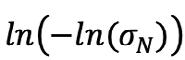
For the WE model, region splitting is done via the apparent activation energy Qc*. Mapping vs , changes in linearly fitted gradient indicate a change in mechanism. Fitted values of Qc* can be used to directly infer the creep mechanism [22].

2.3. Error

Error values are calculated such that: where PLM is equivalent to Qc and is determined by mapping log(tr) vs. 1/T at constant stress. CLM is a constant. For the analysis conducted here, PLM shall be restricted to the form: where A1–4 are non-zero constants. This solution comes from British Standard BSI PD 3525 (1990) and has been widely implemented throughout the field of creep modelling.

Error values >0 means the model underpredicts the rupture time and is therefore conservative. Error values <0 means the model overpredicts the rupture time and could result in unexpected premature failure of components.

R2 is the square of the Pearson product moment correlation coefficient for datapoints x and y. In this work it is used as measure of error when fitting creep model parameters:

3.1. Larson–Miller (LMP) Models

For IN740H, ASME [1, 4] and Render et al. [23] have published LMP models. When examining the original dataset, there are four data points at 650 °C which are outliers. These outliers have rupture elongations of ~20-30%, which is significantly larger than the rupture elongations of 2–6% seen in the other tests at 650 °C. On closer inspection, these data points are for material P2 which is noted not to conform to code case conditions. Examining the higher temperature tests, P2 produces similar elongations and rupture times to other materials. In this work, the four outlier data points at 650 °C have been removed and the LMP refitted using the same procedure as the ASME and Render models with results designated ‘Gray’. The fitting parameters of each LMP model are shown in Table 2.

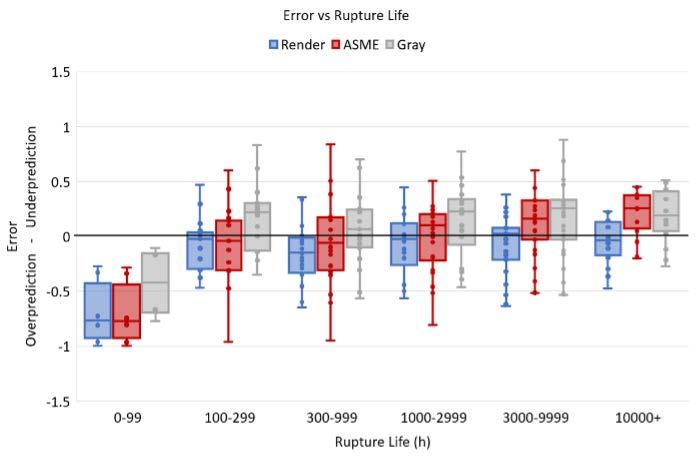
From Table 2 we see that the three LMP models have similar PLMP R2 values and therefore similar accuracies when looking at their ability to predict time to rupture, tr, only. Looking into the source of the error in the models, Figure 1 shows the error in predicting tr with respect to stress, temperature and length of rupture time.

In Figure 1, looking at the Render LMP model the median error values show the model likely to overpredict across all stresses, significantly overpredict at the highest temperature, and be fairly stable/accurate over increasing rupture times. In terms of spread of error, the best fits for stress are seen for 100–400 MPa. Either side of 775 °C the spread of error (inter-quartile ranges) increase. For rupture times > 100 h the interquartile range remains fairly consistent and accurate.

For the ASME LMP model the median error underpredicts for stresses <400MPa then overpredicts at higher stresses. For temperature it underpredicts from 700–825°C, overpredicting at the lowest and highest temperatures showing a similar trend to all the LMP models considered. In terms of rupture time, the ASME LMP model has a linear trend towards increasing underprediction with longer times. Similar to the Render LMP model, the spread of error with respect to stress sees the smallest spread in the mid stress range. For temperature the smallest error is again at the mid-range of 775°C noting the small amount of datapoints at this temperature. The AMSE LMP also sees a reduction in error spread with increasing rupture time.

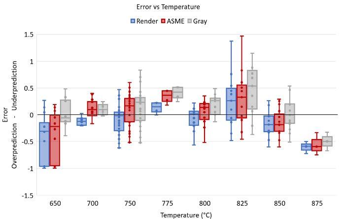
For the Gray model, with the removal of the four outlier datapoints when fitting (model: Gray), it does not show a significant improvement in error with respect to stress. For temperature there are improvements in accuracy at the lowest and highest temperatures. For rupture life, the Gray model trends to a consistent underprediction for rupture lives >100h. There is an improvement in fit for the lowest temperature with decreased error spread and less median error. The overall accuracy of this model is arguably no better than the existing singleregion LMP models, seeing only slight improvements in accuracy in the areas where the four datapoints which were removed lie.

From this analysis, for single-region LMP models:

1. With respect to stress (σ), the single-region LMP models show a trend to overprediction at the lowest and highest stresses.

2. With respect to temperature (T), the single-region LMP models have a significant trend of overprediction, underprediction then overprediction with increasing temperature.

3. With respect to rupture life (tr), the single-region LMP models all trend towards increasing underprediction with longer creep life with the exception of the Gray model, which consistently underpredicts.

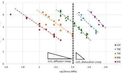
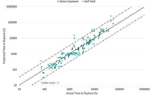
In order to understand the impact of region splitting on the accuracy and model bias, we fit the LMP model using region splitting via stress exponent and via half yield. Figure 2 shows the stress exponent for IN740H obtained by mapping log(tr) vs log (σ). Defining the regions by linear regression fitting, the value of stress exponent (gradient) aligns with the classical interpretation with tests < 251 MPa having a stress exponent linked to diffusion creep, and those > 251 MPa with a stress exponent > 5 experiencing dislocation creep. Therefore, the IN740H data was split into two subsets and the LMP refitted to each subset of data with fitted constants shown in Table 3.

For the half yield region splitting method, it is thought that below half yield the deformation is primarily from creep, whereas above half yield the deformation arises from both creep and plasticity [21]. The yield strength used in this analysis was obtained from Barbadillo et al. [24] for some of the samples listed in ASME [4] where the average yield was found at 0.71 σUTS (0.63–0.81). Half yield was thus taken be 0.355 σUTS for the average temperature dependent σUTS. The LMP constants for the regions are shown in Table 4.

Looking at the PLMP R2 values in Table 3 and 4, there are measurable reductions in model error for the two higher stress regions but an increase in error for the lower stress regions. Looking into the sources of this error, Figure 3 shows the error in predicting tr with respect to stress, temperature and length of rupture time for both region splitting techniques compared to the single-region LMP Gray for reference (also depicted in Figure 1).

From Figure 3 we can see how region splitting affects creep model error. In terms of stress, both region split models performed worse in the lower stress regions as expected from the PLMP R2 values in Table 3 and 4.

For the LMP model region split by stress exponent (n), the model performs slightly better than the singleregion LMP models for the higher stress region with more accurate mean error and narrower spread in error. Overall, the mean error is similar in magnitude to the single-region ASME model with the contrast that the ASME model generally overpredicts whereas the model region split by stress exponent underpredicts. In terms of temperature, the region split model performs better at lower temperatures with increasing variation in error at higher temperatures. In terms of rupture life, the region splitting by stress exponent sees greater accuracy at short lives and trending towards overprediction with longer rupture life contrary to the single-region LMP models in Figure 1c.

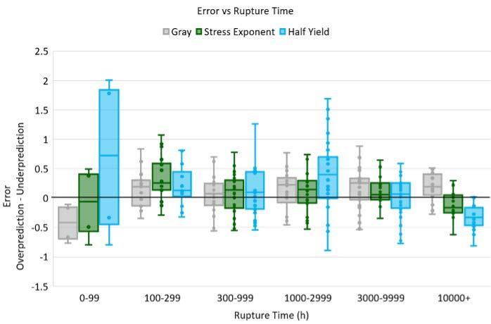
For the LMP model split by half yield, in terms of stress, mean error is generally better but error spread is worse. In terms of temperature, this region split model follows similar behaviour to the other region split LMP model with increasing variations in error with increasing temperature. In terms of rupture life, region splitting via half yield improves the mean error for the bulk of the data with a trend towards underprediction at the shortest and overprediction at the longest rupture lives. For region split LMP models:

1. With respect to stress, region split LMP models show less accuracy at lower stresses and more accuracy at higher stresses when compared to single-region LMP models.

2. With respect to temperature, the region split LMP models have better mean error overall but have increased errors and underprediction for 825°C.

3. With respect to rupture time, the region split LMP models are slightly more accurate with increased rupture time compared to single-region LMP models. Also the region split LMP models trend towards overprediction whereas the single-region model trend towards underprediction with increasing rupture time.

3.2. Wilshire (WE) Models

For the Wilshire model, Render et al. [23] fitted a singleregion model which was unaffected by the removal of the four outlier points mentioned previously. As such the single-region WE constants used are listed in Table 5.

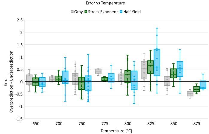
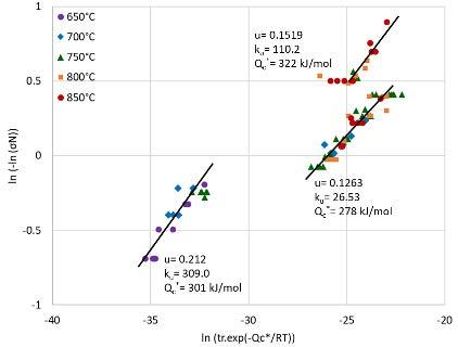
For the region split WE, the data was split according to Qc* via linear regression. The splits and resultant fitted constants are shown in Figure 4. This resulted in three regions being identified with Qc* R2 significantly lower than seen in all other models (Table 6). Figure 5 shows the error of the WE and region split WE with respect to stress, temperature and length of rupture time.

For the single-region WE model, Figure 5 shows different behaviour compared to the LMP models. In terms of stress, the single-region WE model shows consistent mean error that trends to neither over or under prediction. The largest errors are seen for the highest stress tests with overall error comparable in magnitude to the single-region LMP models. With respect to temperature the Wilshire models are inherently different to the LMP models as they evaluate the activation energy for a normalised stress which is temperature dependent. The single-region WE overall has better mean error except for at 825°C and a larger spread of error than the single-region LMP. When considering rupture time, the single-region WE performs consistently well across all rupture lives with no distinct trend to overprediction or underprediction.

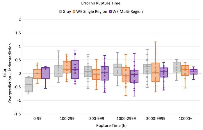
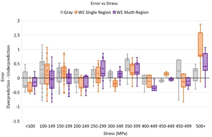
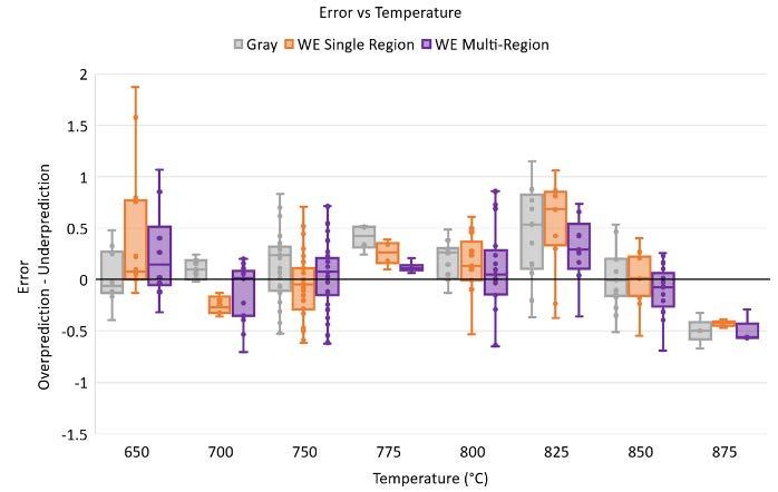
For the region split WE model, in terms of stress the model produces a lower mean error but with a larger spread than the single-region LMP models. The region split WE also trends from slight overprediction to slight underprediction with increasing stress. Both WE equations perform poorly at the highest stress tests with significant underprediction. The region split WE produces the least error with respect to temperature of all models. Like all models examined, it overpredicts at the highest temperatures. In terms of rupture life the region split WE is the most accurate and has no obvious bias towards over or under prediction with longer rupture times, unlike all the LMP models.

For the WE models:

1. With respect to stress, the WE models do not have an obvious trend towards over or underprediction. They perform poorly at the highest stresses. The region split WE model has the most accurate mean error of all models but not the smallest spread in error.

2. With respect to temperature, the WE models perform similar to the single-region LMP models.

3. With respect to rupture life, the region split WE has the least mean error and spread in error. Both WE models produce consistent errors for all rupture lives with no discernible trend towards over or underprediction unlike LMP models.

4. Post Assessment Tests and Extrapolation

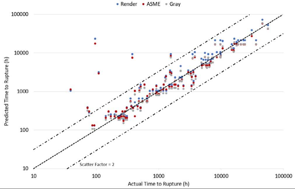
If we examine the European Creep Collaborative Committee Post Assessment Tests (PATs) [25], which determine if a model fit is acceptable, for creep rupture there are three criteria. The criteria are the physical realism of the isothermal data lines, the effectiveness of the model prediction in the given data range, and the repeatability and stability of extrapolations. Modelling techniques used in this paper were chosen to attempt to satisfy the first criteria. For the second criteria, we examine Figure 6 which shows the scatter plots of the predicted and actual time to rupture values. From the scatter plots it can be seen there are only small differences between results, with the LMP models having slightly smaller scatter than the Wilshire plots. These plots are commonly used but provide limited information compared to the above analysis.

For the last criteria of the PAT we need to examine the 100kh rupture strength predictions. Table 5 shows the 100kh creep rupture strengths predicted by each model for the minimum temperature with ≥10% of datapoints (Tmin,10%), the temperature with the most datapoints (Tmain) and the maximum with ≥10% of datapoints (Tmax,10%).

From Table 5, the ASME and Half Yield models experienced turnbacks, never reaching a prediction for 100kh. At Tmin,10% there is a range of strengths with a variation of 29 MPa. For Tmax,10% the range of strengths was 14–27MPa, where available. For Tmain the range of strengths varies by 37MPa from 124–161 MPa. Unfortunately, the true accuracy of the models and whether they comply with the ECCC PATs cannot be fully determined as there are no datapoints at 100kh. Therefore, this raises the question of which model is most likely to produce the most accurate prediction.

From the analysis conducted here we are better able to choose which model is more likely to give a more accurate answer. From Figures 3b, 4b and 5b, with respect to temperature the values for 650°C and 750°C will likely be more accurate than the predicted values for 850°C. From Figures 3c, 4c and 5c, with respect to long rupture lives, it is expected the Render LMP models will overpredict rupture strength whilst the Stress Exponent LMP will likely underpredict rupture strength. The Region Split WE model is the most likely to be the most accurate, but a slight underprediction of the rupture strength is also expected.

5. Discussion

In this article we employ region splitting without examining if the region splits align with changes in creep mechanism or whether the region splits arise from model failure. Looking closer at IN740H, it has ~0.16, ~0.13 and ~17.2% wt. of MC, M23C6 carbides and γ’ precipitates respectively [25]. Looking at the microstructural investigations of IN740H after creep testing, we see at 800°C, 160MPa, 2700h and 850°C, 100MPa, 3000h there is significant growth of the γ’ precipitates. At 750°C, 265MPa, 3147h we do not see this same growth with the γ’ precipitates half the size of those found in the previous creep tests [26]. This change in behaviour occurs at σN <0.2 where for σN <0.2 Qc* = 301 kJ/mol drops to Qc* = 278 kJ/mol for 0.2 < σN < 0.4. This is consistent with what was observed for Grade 22, 23 and 24 P91 steel by Whittaker [22] where the lowest region had a higher activation energy than the midrange region. From further investigations [22] this was linked to the dominant behaviour in the lower region being microstructural evolution, then in the mid-range diffusion becomes the dominant mechanism. Looking at IN740H we see the same behaviour as the lower activation energy for 0.2 < σN < 0.4 is consistent with that for Ni bulk diffusion or diffusion based creep [27] noting it is also consistent with the observed microstructure at 750°C, 265MPa, 3147h.

One of the other models to note is the region splitting by half yield. For the half yield method, half yield is meant to represent the elastic limit and occurs at 0.355σUTS or σN = 0.36 for IN740H. For the WE region splitting method which is not constrained we get a regression fit with a break at σN >0.4 with an activation energy consistent with dislocation creep of Qc* = 322 kJ/mol [28]. This splitting into subsets at σN =0.4 is common for the model that has the least temperature and possibly stress-dependent error (half yield), and the model with the most accurate long rupture life prediction (WE region split).

6. Conclusion

Modern creep datasets often have fewer datapoints for shorter times, meaning extrapolation is critical. In this article we examine a range of creep models and their error profiles with respect to stress, temperature and rupture time. The single-region LMP models performed well. Region splitting the LMP models by stress exponent or half yield did not show significant improvement. The WE model performed to a similar level of accuracy with slightly different error profiles. When predicting 100kh rupture stresses for a dataset without 100kh results, the analysis of the model error profiles allowed for critical evaluation of which strengths were more likely to be accurate. Understanding the model errors in more detail with respect to stress, temperature and rupture time could provide users with insight when extrapolating beyond existing data.

References

[1] ASME Boiler & Pressure Vessel Code Section I Code Case 2702, 2017.

[2] Materials for Advanced Ultra-supercritical (A-USC) Steam Turbines – A-USC Component Demonstration, Pre-FEED Final Technical Report, DOE Award Number DE-FE0026294, 2016.

[3] Solar Energies technology Office, Office of Efficiency & Renewable Energy, U.S. Department of Energy, https://www.energy.gov/eere/solar/receiver-rdcsp-systems , Accessed July 2022.

[4] Boiler Materials for Ultra-Supercritical Coal Power Plants, Final Technical Report, DOE Award Number: DE-FG26-01NT41175, 2015.

[5] NIMS Creep Datasheet 3B.

[6] NIMS Creep Datasheet 11B.

[7] NIMS Creep Datasheet 36B.

[8] NIMS Creep Datasheet 14B.

[9] NIMS Creep Datasheet 15B.

[10] Z. Abdullah, V. Gray, M.T. Whittaker, K. M. Perkins, “A Critical Analysis of the Conventionally Employed Creep Lifing Models”, Materials 7(5):3371-3398, 2014.

[11] R. Swindeman, M. Swindeman, B. Roberts, B. Thurgood, and D. Marriott: DOE/ID14712-1, United States (OSTI.gov), November 2007.

[12] S. Holmstrom, “Engineering Tools for Robust Creep Modelling”, Dissertation, VTT Publications 728, 2010.

[13] M. Kassner, M.T. Perez-Prado, “Five Power Law Creep”, FundamentalsofCreepinMetalsandAlloys , 2004.

[14] B. Wilshire, P.J. Scharning, “A new methodology for analysis of creep and creep fracture data for 9%–12% chromium steels”. InternationalMaterials Review53:91-104, 2008.

[15] V. Foldyna, Z. Kubon, A. Jakobova and V. Vodarek, “Development of Advanced High Chromium Ferritic Steels”, Microstructural Development and Stability in High Chromium Ferritic Power Plant Steels”, TheInstituteofMaterials , pp. 73-92, 1997.

[16] V. Gray, M.T. Whittaker, “The changing constants of creep: A letter on region splitting in creep lifing”, MaterialsScienceandEngineeringA , 632, 2015.

[17] F.C. Monkman, N. J. Grant. “An empirical relationship between rupture life and minimum creep rate”. Deformation and Fracture at Elevated Temperatures.Boston: MIT Press; 1965.

[18] F. H. Norton. TheCreepofSteelsatHighTemperatures. New York: McGraw-Hill, 1929.

[19] S. A. Arrhenius.“Über die Dissociationswärme und den Einfluß der Temperatur auf denDissociationsgrad der Elektrolyte” . Zeitschrift für Physikalische Chemie.4. 1889.

[20] F. R. Larson, J. Miller, “A time-temperature relationship for rupture and creep stresses”. Transactions ASM 74:765-775, 1954.

[21] K. Kimura, “Creep Rupture Strength Evaluation with Region Splitting by Half Yield”, Proceedings of theASME2013PressureVessels&PipingDivision Conference , 2013.

[22] M.T. Whittaker, W. J. Harrison. “Evolution of the Wilshire equations for creep life prediction”. Materials at High Temperatures 31(3):233-238, 2014.

[23] M. Render, M.L. Santella, X. Chen, P.F. Tortorelli, V. Cedro III, “Long-Term Creep-Rupture Behavior of Alloy Inconel 740/740H”. Metallurgical and MaterialsTransactionsA , April 2021.

[24] J. de Barbadillo, A. Di Gianfrancesco. “Materials for Ultra-Supercritical and Advanced UltraSupercritical Power Plants: INCONEL alloy 740H”, 1st ed., Woodhead Publishing, pp. 469–510, 2017.

[25] S. Holdsworth. "The European Creep Collaborative Committee (ECCC) Approach to Creep Data Assessment." ASME. Journal of Pressure Vessel Technology , 130(2) 2008.

[26] S. Zhao, F. Lin, R. Fu, C. Chi, X. Xie, “Microstructure Evolution and Precitpiates Stability in Inconel Alloy 740H during Creep”, Advances in Materials Technology for Fossil Power Plants , ASM International pp.265, 2014.

[27] M. F. Ashby, “A first report on deformationmechanism maps”, ActaMetallurgica20(7), 1972.

[28] M. T. Whittaker, W. J. Harrison. C. Deen, C, Rae, S. Williams, “Creep Deformation by Dislocation Movement in Waspaloy”, Materials10(1): 61 2017.

Foreword

The Fatigue 2024 conference will bring the international fatigue and durability community together to share knowledge and understand the challenges in using sophisticated engineering simulation, characterisation and modelling tools to complement sound test programmes and develop reliable and cost effective products for modern usage.

As engineering modelling and simulation tools become ever more powerful and sophisticated there still remains the challenge of correlating the virtual world with both idealised laboratory testing and the wide, and potentially unexpected, range of service conditions experienced by machines and structures. These challenges are compounded by the advent of new materials, new ways of manufacturing components, new applications and new test, measurement and characterisation techniques.

We will seek to explore not only the latest developments in engineering modelling and simulation, new test, measurement and characterisation techniques, innovations in manufacturing and developments in materials science, but also the complex interrelations between all these topics that give rise to improvements in fatigue performance, durability and structural integrity.

The 3 day conference builds on the longestablished philosophy of the Engineering Integrity Society to provide a forum for practising engineers and researchers to exchange ideas and experiences in all aspects of structural integrity. Contributions will be welcomed from all disciplines; from academia, industry and research organisations. As well as giving practitioners an opportunity to keep up-todate in the latest developments in durability of materials and structural analysis techniques, the conference will provide an excellent forum for researchers to promote their work and enhance its transfer to, and impact on, industrial applications.

Venue

The conference will take place at Jesus College, Cambridge, UK. Set in 24 acres of gardens in the heart of Cambridge, it provides a beautiful setting for events in a purpose-built conference centre. Established in 1496 on the site of the 12th Century Benedictine nunnery of St Mary and St Radegund it is protected from the noise and bustle of the town. The College has many notable buildings dating as far back as the 12th Century and the spectacular Hall with its vaulted ceilings provides a unique dining venue for our conference dinner.

Call For Papers

We are interested in high quality papers in all aspects of the fatigue and durability of engineering materials, www.fatigue2024.com machines and structures.

In particular:

• Innovations in experimental techniques for fatigue characterisation

• Developments in modelling fatigue including:

∼ multi-scale and multi-physics

∼ neural networks and machine learning

∼ stochastic methods

• Durability of advanced materials

• Integrity of recycled and reprocessed materials

• Joining technologies: bolts, welds, adhesives, joining dissimilar materials, correlation of testing and in-service durability

• Surface engineering and durability

• Innovations in digital imaging

• Fatigue in adverse environments, such as high temperatures, corrosion and/or embrittling species

Authors of suitable papers will be invited to submit extended manuscripts to selected peer reviewed international journals. More details will be available on our website.

The abstract should contain:

• Title of the paper

• Authors (full address of the company, email, personal titles of the corresponding author and co-authors)

• Statement of contents and main points

The abstract should clearly emphasise the main scientific, technical, economic or practical aspects of the paper.

Key Deadlines

Submission of abstract - 30 April 2023

Acceptance of abstract - from May 2023

Full papers received by - 30 September 2023

Proceedings And Exhibition

All accepted papers will be included in the conference proceedings. The proceedings containing the full texts will be distributed to delegates at the conference.

An exhibition of material testing equipment and other fatigue related services is planned. Interested companies should contact the Conference Secretariat.

Peter Watson Prize

The Peter Watson Prize will be awarded to the best presentation given by a young engineer. Entrants should meet at least one of the following criteria:

• A person working in industry below the age of 28 on submission (potential entrants please provide date of birth with abstract)

• A post-doctoral worker with a maximum of 3 years’ experience since completing a PhD/EngD

• Any currently registered undergraduate or postgraduate student

Submission Of Papers

You are kindly requested to submit an abstract (one A4 page maximum, only in pdf format, size smaller than 1MB) to the Conference Secretariat.

International Scientific Committee

Alan Hellier (Australia)

Alberto Campagnolo (Italy)

Alfredo Navarro (Spain)

Ali Fatemi (USA)

André Galtier (France)

Andrea Carpinteri (Italy)

Andrea Spagnoli (Italy)

Barbara Rossi (UK)

Chris Hyde (UK)

Christophe Pinna (UK)

David Nowell (UK)

Ken Wackermann (Germany)

Fabien Lefebvre (France)

Filippo Berto (Norway)

Francesco Iacoviello (Italy)

Francisco A Diaz (Spain)

Frank Walther (Germany)

Harry Bhadeshia (UK)

Hellmuth Klingelhoeffer (Germany)

Hossein Farrahi (Iran)

James Marrow (UK)

James Newman (USA)

Jan Papuga (Czech Republic)

Johan Moverare (Sweden)

Liviu Marsavina – (Romania)

Luca Susmel (UK)

Marc Geers (The Netherlands)

Mark Whittaker (UK)

Martin Bache (UK)

Matteo Benedetti (Italy)

Matteo Luca Facchinetti (France)

Mike Fitzpatrick (UK)

Miloslav Kepka (Czech Republic)

Muhsin J Jweeg (Iraq)

Neil James (UK)

Pablo Lopez-Crespo (Spain)

Paul Bowen (UK)

Phil Withers (UK)

Philippa Reed (UK)

Reinhard Pippan (Austria)

Rob Ritchie (USA)

Robert Akid (UK)

Sabrina Vantadori (Italy)

Shahrum Abdullah (Malaysia)

Svjetlana Stekovic (Sweden)

Takashi Nakamura (Japan)

Thierry Palin-Luc (France)

Veronique Doquet (France)

Wim de Waele (Belgium)

Yee Han Tai (UK)

Yoshihiko Uematsu (Japan)

Youshi Hong (China)

Yukitaka Murakami (Japan)

Local Technical Committee

Dr Amir Chahardehi

Andrew Blows

Assoc Prof Chris Hyde

Dr Emilio Martínez-Pañeda

Dr Fabien Lefebvre

Dr Farnoosh Farhad

Prof Filippo Berto

Prof Francisco A Diaz

Dr Hassan Ghadbeigi

Dr Hayder Ahmad

Dr Hollie Cockings

Dr John Yates

Prof Mark Whittaker

Dr Mohamed Bennebach

Dr Pablo Lopez-Crespo

Paul Roberts

Dr Peter Bailey

Robert Cawte

Dr Spencer Jeffs

Assoc Prof Svjetlana Stekovic

Yi Gao

CONFERENCE CONVENOR Dr John Yates

DEPUTY CONVENOR Dr Hollie Cockings

CONFERENCE SECRETARIAT

Sara Atkin

Engineering Integrity Society

6 Brickyard Lane, Farnsfield

Nottinghamshire, NG22 8JS, UK

Tel. +44 (0)1623 884225

Email: info@e-i-s.org.uk

Website: www.fatigue2024.com