New life for your assets

Nigel Curson, Alastair McLachlan and Aidan Charlton, Penspen Limited, UK, present a statistical derivation of the present value (PV10) of a step-out development based on remaining life.

The oil industry uses the PV10 value to evaluate hydrocarbon assets. It is a calculation of the present value of estimated future hydrocarbon revenue, less direct expenses. It is discounted to the present using an annual rate of 10%. In practice, when applied to a post plateau and declining oil or gas reservoir connected to a host platform or processing facility by a relatively long pipeline, the PV10 value is limited by the asset’s remaining life, including pipelines and wells. Having to intervene for a repair or access to a well with declining

revenue can lead to the end of the economic life of an asset or field. However, appreciating that a producing asset comprises various critical components, this article mainly concentrates on the pipeline asset. Understanding the condition and opportunity of the pipeline as a distinct asset has the potential to realise future value.

Several standards guide the fitness for service (FFS) of pipelines, including DNVGL-RP-F101,1 ASME B31G,2 and the Pipeline Defect Assessment Manual (PDAM).3 Some standards specifically address remaining life assessment, such as ISO TS 12747,4 and NORSOK Y-002.5 These standards tend to focus on technical integrity.

NORSOK Y-002 uses the term ‘integrity level’ and defines it as the absence of risk. It notes that risk in this context has various aspects, varies with failure mode, criticality, and system type. It describes it as not being a variable but having lower and upper bounds and an acceptable level. It does not explain how it is derived and indicates it can never be fully known. ISO 16708 takes a more general approach across the whole life cycle and is more tangible in its use, in that it provides target failure probabilities based on fluid category, location (proximity of people) and safety class.6 An offshore oil pipeline is classed as ‘normal safety class’, which for an ultimate limit state is assigned an acceptable failure probability of 1x10-4 or 1/10 000 per km, per year.

In practical economic terms the remaining life is determined when adding more years of operation reduces net present value. In other words, the present value of direct expenses exceeds the present value of the operation. This is typically driven by the need to intervene to undertake expensive repairs or replacement. This can be driven by inspection data and/or a perception of risk.

Most remaining life methodologies systematically identify credible failure mechanisms such as corrosion and fatigue. They then use historical data, such as inspection data or operating conditions, to determine the degradation rate. The degradation can be expressed in terms of corrosion growth rate, fatigue life reduction, or possibly crack growth rate. This is combined with a FFS assessment to determine when risk in the future becomes unacceptable, and where intervention/repair or decommissioning is required. Inspection and monitoring are used to determine the rate of degradation and track progress against the prediction. More sophisticated methodologies, such as implemented within the Penspen THEIA platform take actual live data and use this to dynamically calculate the remaining life.7 This creates value for the operator, e.g. tactical value (small value pool) with a quicker route and more confidence in the optimal operational solution, and strategic value (big value pool) with deferred capex and the avoidance of failures.

Design life Pipelines are typically designed for 30 years and many are now operating considerably beyond their original design life. The safe operation of pipelines in the North Sea is controlled by a series of regulations that requires the assessment and management of risk. This is carried out by the pipeline operator implementing a rigorous pipeline integrity management system (PIMS).

The design life is chosen to prevent failure during operation due to time-dependent degradation mechanisms such as corrosion and fatigue. This assumes a degradation rate in the design phase. When the pipeline reaches the end of its design life, this does not mean the pipeline should immediately be decommissioned because it is now representing an unacceptable risk. In practice, considerable investment has been made in managing the pipeline in operations, performing inspections and implementing mitigations. In practice: ) The corrosion rates and fatigue rates established during the original design process may prove to have been conservative.

) Defects could have been repaired.

Extending the pipeline’s life might have considerable business advantages due to remaining recoverable hydrocarbons, pipeline change of use or exploiting the possibility of third parties using the asset for their product. It may even make the asset attractive to potential buyers. These last aspects are now covered by UK legislation. The strategy for maximising economic recovery in the UK (MER UK) came into force in March 2016.8 This obliges all stakeholders to maximise the expected net value of economically recoverable petroleum. If a party decides not to do this, it must allow others to use its license or infrastructure, including pipelines.

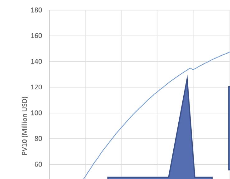
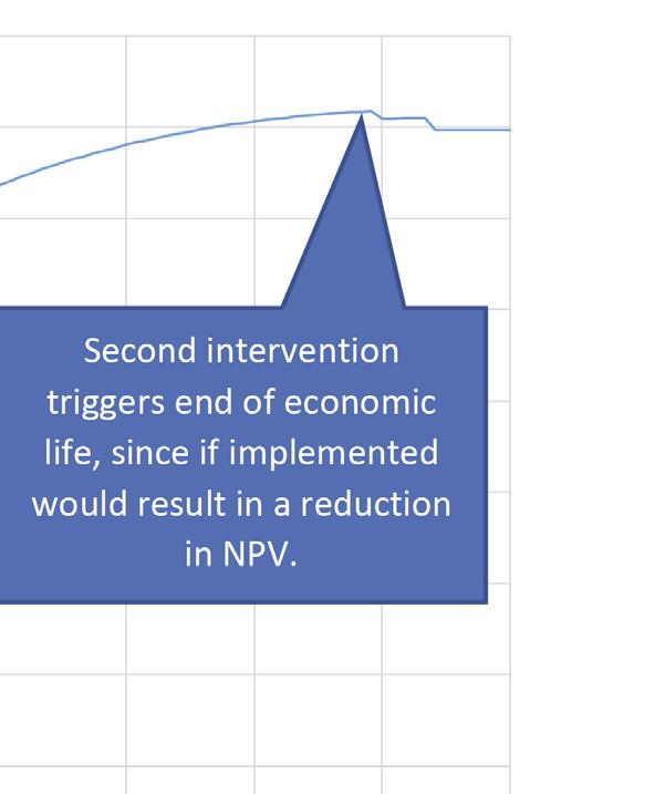
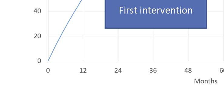
Figure 2. Cumulative PV10 per month of operation.

Asset life extension (ALE) process The concept of life extension is to increase the asset’s life but still maintain an acceptable risk. This would normally consider changes not considered in the original design, including changes in: ) The integrity of the asset through the development of flaws from corrosion or fatigue.

) Fluid compositional or flowrates.

) Environmental loading.

) Temperatures and pressures.

Corrosion is usually the most significant degradation mechanism for pipelines. Typically for offshore pipelines, this is on the inside of the pipeline since anodes are quite good at controlling external corrosion. However, anodes do occasionally require replacement. The uncertainty associated with corrosion rates is an important factor. ISO 12747 states that the degree of uncertainty in the calculated corrosion rate (and therefore the remnant life) should be determined by calculating upper and lower bounds.4

ALE goes beyond just estimating the remaining life of the asset, but also includes organisational requirements in terms of competencies, continuous operability of safetycritical equipment, updating inspection and monitoring requirements, legislation requirements and updating PIMS documentation.

Remaining life optimisation In general, the risk associated with operating a pipeline increases with time and accelerates as they approach the end of their life. If the predicted remaining life is not enough to satisfy the overall field economics due remaining reserves, there will be a need to consider alternatives. These can include: ) Replacing the pipeline or parts of it.

) Repairing parts of the pipeline.

) Downrate to operate at a lower pressure.

) Use of inhibitor to reduce the corrosion rate.

) To change the composition or flowing conditions to reduce the corrosivity of the product.

) Increasing inspection frequency to carefully manage the risk associated with operating an asset towards the end of its life.

Having the capability to model these ‘what if’ scenarios quickly will drive the optimum forward plan. The THEIA platform has this forecasting perspective and capability.

Effective maintenance strategies The last bullet point from above is important. Inspection and the subsequent actions for pipelines can be classified as condition-based maintenance. The actual condition of the asset is used to determine what maintenance needs to be performed. Inspection using an intelligent pig is expensive, takes time

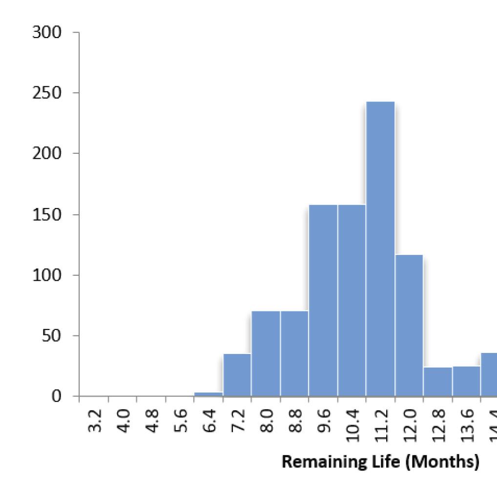
Figure 3. Statistical distribution of remaining life.

Figure 4. Statistical distribution of PV10.

Table 1. Distribution for principle variables Value Mean Standard deviation Resultant max value Resultant min value

Oil price (US$/bbl) Production decline (per annum) Repair cost and inspection cost (million US$) 30 5 44.1 11.6

10% 2% 16% 4%

5 0.5 6.7 3.6

Corrosion rate (mm/y)

) A cost model which includes the cost of a repair and associated inspection linked to the integrity of the pipeline. .3 .06 .49 .13 The cost model calculates the revenue, costs and contributing NPV each month, to procure and can be disruptive to operations. The taking account of degradation and required intervention opportunity here is to use predictive maintenance as a to repair. The end of life is triggered when the forwardsupplement to inspection to optimise decision making. looking NPV is low or negative, normally coinciding with a This would include highly efficient inspection matching required intervention. This is illustrated in Figure 2. routines to predict corrosion growth rates and confidence Running the model on a deterministic basis (no levels along the pipeline, use of real-time data including variation in inputs), gives a remaining life of 10.8 years and pressure, flowrates and temperatures to give live updates an NPV of US$250 million. of remaining life on a dashboard, along with other KPIs to Using Monte Carlo simulation and varying the main enable mitigating actions to be taken as required. These parameters of oil price, annual decline and corrosion rate, tools are implemented within THEIA which is based on an an NPV with a median of US$246 million and a standard industrial analytics platform. deviation of US$66 million and a remaining life with a median of 10.2 years and a standard deviation of 1.9 years Net present value (NPV) modelling are produced. The distributions are shown in Figures 3 and It is hard to compare all the above options directly since 4, with reasonable probabilities that remaining life and they all have different investment and revenue profiles PV10 could be 8.0 years and US$180 million respectively. with time. A good way of comparing them is to calculate The variations used are given in Table 1. the NPV of each, where all the income (cash outgoings) and investments (cash outgoings) are netted and brought Conclusions back to a value today (present value). The option with the Use of an NPV model such as implemented within THEIA highest NPV is the most attractive. to quickly compare remaining life options is considerably

Most applications of NPV are assessed on a superior to a deterministic assessment and provides deterministic basis where the answer is one value. This is valuable insights into the possible variations. necessarily conservative. In practice, the rate of decline, An insight from the above model is the fact that the the rate of degradation and oil/gas price are not fixed changes in remaining life, where the reduction in revenue values. All these values can vary considerably. due to reduced production is in line with degradation,

This article considers a hypothetical oilfield, based are not that significant in NPV terms. This is because the on the typical North Sea step out development (Figure 1) majority of NPV contribution has been in the early life. with declining production and an ageing pipeline. It uses Where remaining life optimisation will have a more statical analysis to calculate the possible variation of significant impact on NPV will be where production is still PV10, taking account of the variation of oil price, decline at a high level, but the oil price is low, income is low and in production, degradation rate, cost of inspection and investment decisions are deferred or where a replacement cost of repair intervention. pipeline dictates the end of economic life.

Reservoir decline is based on Arp’s decline analysis model.8 Statistical analysis is based on Monte Carlo References Simulation. 1. DNVGL. RP-F101 Corroded Pipelines. 2. ASME. B31G - 2012(R2017) Manual for Determining the Remaining Strength of Corroded Pipelines. Economic model 3. Penspen Limited. Pipeline Defect Assessment Manual Version 2, a Joint The economic model used has three components: Industry Research Programme. 4. ISO. TS 12747:2011 Petroleum and natural gas industries – Pipeline ) A revenue model which assumes an initial production transportation systems – Recommended practice for pipeline life extension. rate, a decline in production per year and the oil price. 5. NORSOK. Y-002 Life extension for transportation systems (Rev. 1, December 2010). 6. ISO. 16708: Petroleum and natural gas industries, Pipeline transport systems, ) A cost model which uses a fixed price for the Reliability-based limit state methods. 7. Penspen Limited. THEIA - Cloud Based Integrity Tools and Industrial Analytics. organisation, a price per barrel of oil price for 8. Arps, J.J. Analysis of Decline Curves, SPE-945228-G, 1945. production chemicals, the cost for intelligent pigging 9. Oil and Gas Authority, UK. The Maximising Economic Recovery Strategy for and General Visual Inspection (GVI) based on a set the UK. 10. ISO. 13623 (2000): Petroleum and Natural Gas Industries - Pipeline frequency in numbers of years. Transportation Systems.