Optimization of Lubricant Design through Use of Design of Experiments Methodology

By: Jason Galary Applied Science and Tribology, Nye Lubricants, Inc. Department of Mechanical Engineering, University of Massachusetts Dartmouth

A new automotive lubricating grease was formulated using polytetrafluoroethylene (PTFE) to thicken polyalphaolefin (PAO) base oil. This grease was developed to meet targets for rheology and protection against wear for automotive applications. The formulation was developed and the manufacturing process was optimized using computational data analysis instead of a more typical trial-and-error approach. The computer data analysis methodologies were design of experiment (DOE), regression analysis (RA), and evolutionary algorithm (EA).

In this study, a DOE methodology was employed to optimize the process of designing a lubricating grease. Typically, a lubricant is designed through use of a combination of technical knowledge, prior experience, and trial-and-error experimentation to develop a starting point for formulation and processing conditions. Then, modifications are made along the way to improve the formulation and processing procedures. While this methodology will get the job done, it may take longer and produce a less optimum product than one created through a DOE methodology.

This study illustrates the benefits of a well-laid-out DOE plan to design a new PAO-PTFE formulation for the lubrication of automotive steering shafts and other components. Data from the DOEs were analyzed by RA to construct empirical models. Then, some models were optimized using an EA. The final results were predictions of the optimal formulation and manufacturing procedures for this grease. These predictions were compared with data for validation. Results from this study support the application of DOE, RA, and EA methodologies to develop formulations and manufacturing procedures.

Introduction

There are many goals to be considered when designing a new product. During the development of any material or product, careful attention must be paid to raw materials, manufacturing process, and validation testing. However, it is not always feasible to perform extensive experimental designs including all the validation testing for every possible variable due to time and cost constraints. Many times in industrial laboratories, future generations of products are developed by modifying existing ones, which inherit their advantages (and sometimes their problems). This creates a situation where a new formulation is not optimized and scaling up is difficult because it is not optimum for the new formulation.

A low yield in scale-up or production, cost variances due to increased amounts of raw materials or time, and inconsistent product performance data can occur when a formulation or production process is not robust A robust product or process design is insensitive to changes caused by normal variability.

Background

This study applies a design of experiments (DOE) methodology to develop and optimize a new lubricating grease formulated using a fluoropolymer thickener (polytetrafluoroethylene, PTFE) to bind a polyalphaolefin (PAO) oil. This grease is intended for automotive steering applications. The manufacturing process for these materials can range from very simple mixing to a much more complicated process that involves specialized mixers, homogenizing equipment, and milling processes. A DOE approach was used to develop this product with more control and less variability than typical trial-and-error approaches.

Design of Experiments Methodology - Basics

DOE is a set of tools and guidelines for running experiments in a controlled fashion. DOEs can provide insight into the factors that affect the outcome of a process or product.

In this study, DOE is used to develop the formulation and processing conditions for a PAO-PTFE grease that meets targets for anti-wear and rheology performance.

In this study, the general steps of the DOE methodologies are: 1. Identify variables (also referred to as ‘factors’) that will possibly influence the product/process and its performance. The various factors and levels for the three

DOE are listed below. 1. Wear/Kinematic Viscosity (KV) DOE i. Load (kg): 20, 40, and 60 ii. Speed (rpm): 600, 1,200, and 1,800 iii. Temperature (°C): 25, 62.5, and 100 iv. Kinematic Viscosity (at 40°C, cSt): 30, 115, and 200 v. Wear Additive Concentration (%): 0, 0.5, and 1.0 2. Main Process DOE i. Mixing Type: Single Planetary and Double Planetary ii. Oil Temperature (°C): 25 and 100 iii. PTFE Type (Particle Size, μm): 1 and 5 iv. PTFE Concentration (%): 40 and 50 v. Mixing Time (h): 2 and 8 3. Optimization DOE i. PTFE Concentration (%): 45 and 50 ii. Mixing Time (h): 4 and 12 2. Model Selection: In this part of the study, different DOE models were evaluated for their fit in the experiment and chosen based on trade-offs like time, cost, and importance. 3. Perform DOE: All testing was completed in a randomized order with as many controls as possible in place. 4. Analyze the responses (results of interest from DOE):

Statistical Analysis software (Minitab) was used for this analysis including ANOVA (analysis of variance) and regression to determine the significant factors in the experiments. 5. Perform Computational Optimization: The empirical equations from the regression analysis were used in a purely computational optimization to predict the results of the optimization DOE and illustrate where additional time/costs can be saved with a robust experimental model. 6. Validate Empirical Equation and Optimize

Materials and Methods

Experimental Goals

The primary purpose of this study is to design and develop a new lubricating grease using DOE and optimization methodologies. The key steps in this study are. 1. Utilize DOE and ANOVA to study formulation variables that effect rheology and wear protection of a PAO/PTFE lubricating grease. 2. Use Response Surface Methodology and Evolutionary Algorithms to optimize a grease formulation.

Raw Materials

• PAO 6 and 40 cSt Base Fluids. • Alkylated Phenyl-Alpha-Naphthylamine and Methylene bis (dibutyldithiocarbamate) and tolutriazole derivative Antioxidant Additives • Amine Phosphate and Borate Ester Anti-Wear Additives • Two different types of PTFE, Type A and Type B, with primary particle sizes of 1 and 5 μm, respectively

Grease Preparation

Grease samples were prepared using single and double planetary mixers for combination of the PAO fluid with PTFE powder. Processing of the grease was then finished through a colloid mill with the number of passes controlled for all samples. The number of mixing hours was also controlled to reduce variability in the experiment.

Experimental Methods

• Kinematic Viscosity: Testing was performed according to ASTM D445 using a calibrated glass capillary viscometer. • 4-Ball Wear: Testing was performed according to ASTM D4172 using a Falex Four-Ball Wear instrument. This unit was capable of 60 kg load and 1,800 rpm with a maximum temperature of 150°C. • Apparent Viscosity: Testing was performed using a Brookfield DV-iii Rheometer with a T-B spindle at 1 rpm and 25°C.

Product requirements

• Kinematic Viscosity: Between 80 and 150 cSt at 40°C • 4-Ball Wear: Less than 0.5 mm • Apparent Viscosity: Between 12,000 and 16,000 Poise (P) at 25°C • Cone penetration: NLGI grade 1.5 to 2 (Secondary to apparent viscosity for this application)

Software Tools

For the statistical analysis and DOE work, Minitab 17 was used while the optimization algorithm was written in Matlab.

DOE Approach to Formulation - Details

The purpose of using a DOE approach to the formulation of a lubricating grease is the same as it is in other applications to improve a process, design a material, or solve any scientific problem. Using well-planned and structured experiments combined with statistical analysis, the effects of variables and interactions can be estimated through empirical modeling that

replaces more computationally expensive simulations through a data driven construction [1] [2] [3]. This engineering methodology is used when it is difficulty to directly measure the response of interest. A DOE model is only as good as the data points; they must be valid points and different enough from each other to provide useful insights.

In its simplest form, linear regression analysis helps to explain the relationship between two or more variables through statistical analysis. From this analysis, data based models are created that can be used for prediction of the response to different values of the variable. An example of where this could be used is in the testing of different materials for the exterior of the Space Shuttle. Simulations of air flow, heat transfer, radiation resistance will all have to be performed. Different geometries, materials, etc. will all have to be simulated which could take days, months, or even years.

There were several stages to grease development using DOE in this study. First, the base oil viscosity and the concentration of the anti-wear additive are determined. A Box-Behnken response surface DOE was used to find the optimum viscosity and percentage of an additive package to provide protection from wear. Second, the sources of variation in the manufacturing process and the new product’s rheology were investigated using a full factorial DOE. And third, the grease manufacturing process was optimized.

A key calculation in regression analysis and experimental design is the coefficient of determination (R2). This value represents the proportion of the variance of the dependent variable that is related to the independent variable. The coefficient of determination indicates the correlation between predicted values from an empirical model and the actual values. It also indicates the correlation between the independent variables and the system response. The coefficient of determination is measured on a scale of 0 to 1 which represents no correlation (0%) or complete correlation (100%). This means the closer R2 is to 1, the higher the percentage of variability that is explained by the empirical model.

Experimental Designs

Three different experimental designs were used in this study. First, a Box-Behnken response surface design was used to determine the kinematic viscosity of the base oil and the optimum level of anti-wear additives in the formulation. Second, a fractional factorial design was used to determine the important factors that impact the manufacturing process of the grease and the rheology. Third, a central composite response surface design was used to optimize the manufacturing process to ensure a robust design.

The Box-Behnken response surface design was chosen to determine the kinematic viscosity and the optimum level of anti-wear additive to minimize the wear as tested by ASTM D2266 (4-Ball Wear). This design was chosen instead of a standard central composite response surface as all test parameters were in the design space and the experiment could be performed with fewer runs. Because all of the points of interest in this experiment were within the design space, axial points were not tested due to the limitations of the instrument. This experiment tested the full bounds of the speed, load, and temperature for the 4-Ball equipment used in the experiment. This allowed kinematic viscosity and additive percentage to be researched and optimized for the newly designed product.

After the kinematic viscosity and additive concentration were selected, a 25-1 Half Fractional Factorial DOE was created to model the possible production processes, Figure 1. The type of finish processing was held constant with homogenization and milling. The mixing type was an important variable with single planetary (Hobart) and dual planetary mixing styles being studied. The amount of mixing time, thickener concentration, and the average PTFE particle size were also tested as variables in this study. The final variable studied was the oil temperature when the PTFE was added to prior to mixing.

Because this DOE was a 25-1 half fractional design, it required 32 runs for full resolution. Instead this was run as Half Fractional Factorial DOE design which required only 16 runs. This gives the model a Level IV resolution which maintains full resolution on the main effects but confounds the 2 Way effects. This is not as risky as it would seem due to the hierarchy principle, which states that when two interactions are confounded with one another, the interaction that is the most likely to be significant is the one containing factors whose main effects are themselves significant [5]. This combined with effect sparsity (Pareto rule) which means that only a few of the main factors turn out to be important, allows us to consider a Level IV resolution as low risk. This design will, however, have less resolution of the 3 way effects because they are confounded with the main effects and there is no way to decouple them [5].

The mixing time (prior to milling) was included to help determine the threshold that is needed to make this product consistently homogeneous. The PTFE type and concentration were included in this model as it was expected that these two factors will be part of the optimization of the product. Finally, the oil temperature when the PTFE was added was included to measure the effect of this variable. The experiments were run with two replicates to add resolution to the degrees of freedom in this design. Based on the number of samples tested in this experiment, there was a 95% Statistical Power Level to determine a standard deviation of 1.365σ in the model [5].

Wear Additive Level Selection Results

The results of the Box-Behnken response surface experiment to determine the kinematic viscosity and the concentration of the additives needed for this application provided formulation constraints for this product development. The optimum level for the anti-wear additives was determined to be 0.5% with a kinematic viscosity of 115 cSt. This formulation produced a wear scar of 0.38 mm which was less than the 0.5 mm target.

Contour plots were created to illustrate the effects of speed, temperature, load, and viscosity on the wear rates. Figures 2

and 3 are two-dimensional illustrations of the wear scar area as a function of two variables.

The interaction effect of additive concentration versus speed was linear as the wear scar increased incrementally with the speed, Figure 2. However, the wear increased slightly faster at the highest concentrations of the additive package. The additive temperature contour plot showed a relationship between the temperature, additive concentration, and wear scar, Figure 3. Based on these data and the contour plot, this additive package appeared to be best suited for addition at 75⁰C at a concentration of 0.5% or less.

The contour plot of viscosity and additive concentration showed a strong relationship, Figure 4. The wear was greatest at the extremes of the viscosity and additive concentrations (both high, both low) and least at the opposing corners (high viscosity and low additive concentration, low viscosity and high additive concentration).

In the absence of anti-wear additives, it was expected that there would be more wear for lighter viscosity and less wear for heavier viscosity oils. Without additives, the fluid could provide protection through full film lubrication. The calculated theoretical film thickness was greater than 2 μm for the heavier oil in this study.

In the presence of a high level of anti-wear additives, it was hypothesized that there would be better protection and less wear at low viscosity because of the presence of the additive in the contacts. However, wear would be greater at higher viscosity because there would be less mobility of additives into the contacts.

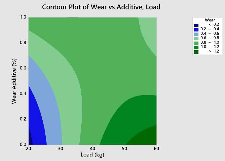
The impact of load on the wear rate is shown in the contour plot in Figure 5. Wear increased as the load increases with no additives, as expected. For loads below 30 and 50 kg and above, the additive package provided more wear protection as the concentration increased. However, at 40 kg, the additive concentration had no significant effect on the level of wear. This result is interesting because 40 kg is the standard load condition for the 4-Ball Wear Test (ASTM D4172).

Based on the application conditions, the contact stresses produced an equivalent load of 40 kg at an average temperature of 75⁰C, and a sliding speed of approximately 800 rpm. The optimum additive level was 0.5% with a kinematic viscosity of 115 cSt. The resulting wear scar was 0.38 mm, which is less than the target specification of 0.5 mm. Figure 1: Cube Plot of Main DOE Factors

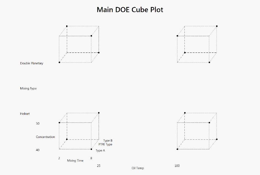
Figure 2: Contour Plot of Wear (mm) vs. Speed (rpm) and Additive Concentration (%)

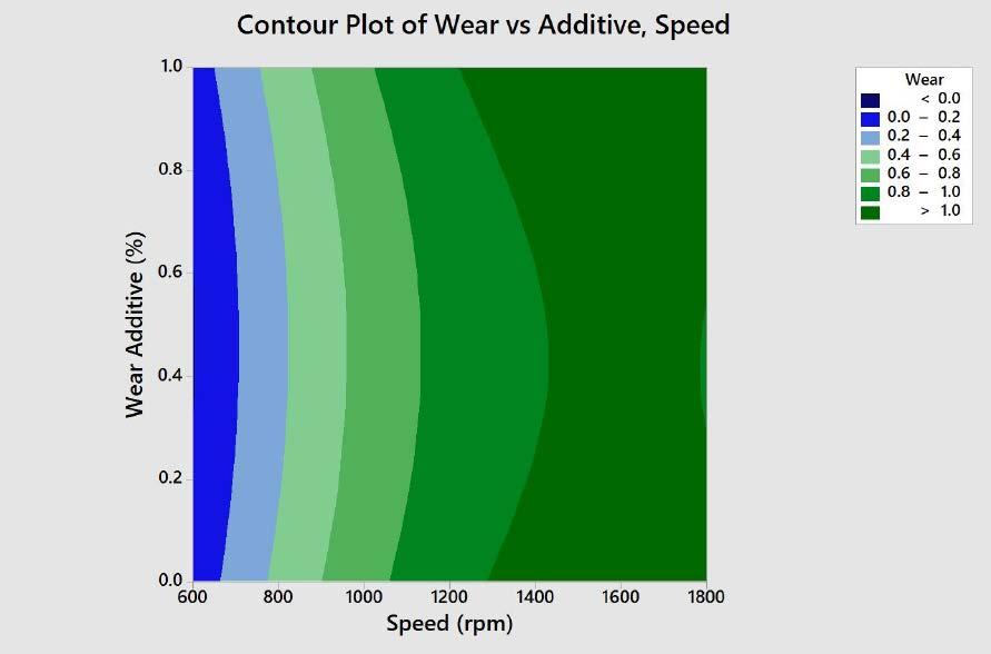
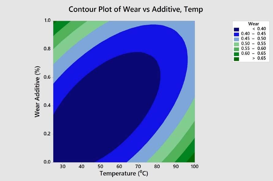
Figure 4: Contour Plot of Wear (mm) vs. Viscosity (cSt) and Additive Concentration (%) Figure 5: Contour Plot of Wear (mm) vs. Load (kg) and Additive Concentration (%)

Main DOE for Product Design

After the DOE to determine the kinematic viscosity and additive concentration was completed, a 25-1 Half Fractional Factorial DOE was performed to model the possible production processes. The type of finish processing was held constant with homogenization and milling. The mixing type was an important variable with single planetary (Hobart) and dual planetary mixing styles being studied. The amount of mixing time, thickener concentration, and PTFE particle size were also tested as variables in this study. The final variable studied was the temperature of the oil when the PTFE was added to prior to mixing.

The initial DOE model was reduced to the final model by eliminating terms that had no statistical significance. This was done iteratively because removal of each factor influenced the calculation of the remaining terms. The terms were removed by the highest order first to help reduce the confounding with the other terms. This new model represented >99.5% of the variation in the design R2. This model also produced the following regression equation where f is the Brookfield apparent viscosity. This regression equation will be used in the computational optimization as the objective function.

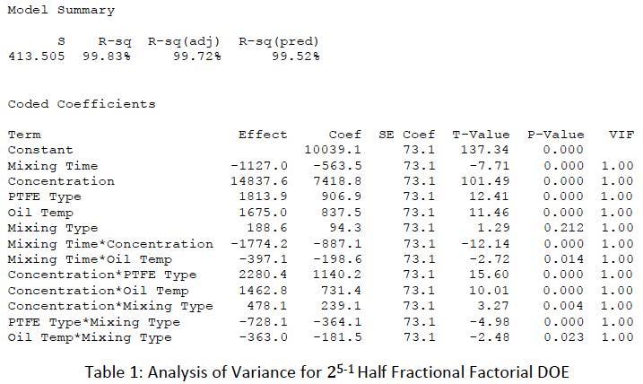
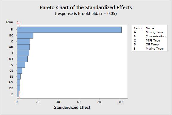
The calculated variance in variation factor (VIF) of 1.0 gives an idea of the severity of multicollinearity, which occurs when two or more variables in a regression model are highly correlated. This means that one variable can be linearly predicted from the other with a high degree of accuracy. From this result, it was shown that there was virtually no correlation between the model terms. This indicated that the model is orthogonal based, as it has a VIF of around 1. Based on the final model, fitted means were then calculated based on the regression equation for all other points in the design space that were not tested. The cube plot with these fitted means is shown in Figure 6. In Figure 7, the Pareto chart of the standardized effects from the final DOE model is plotted.

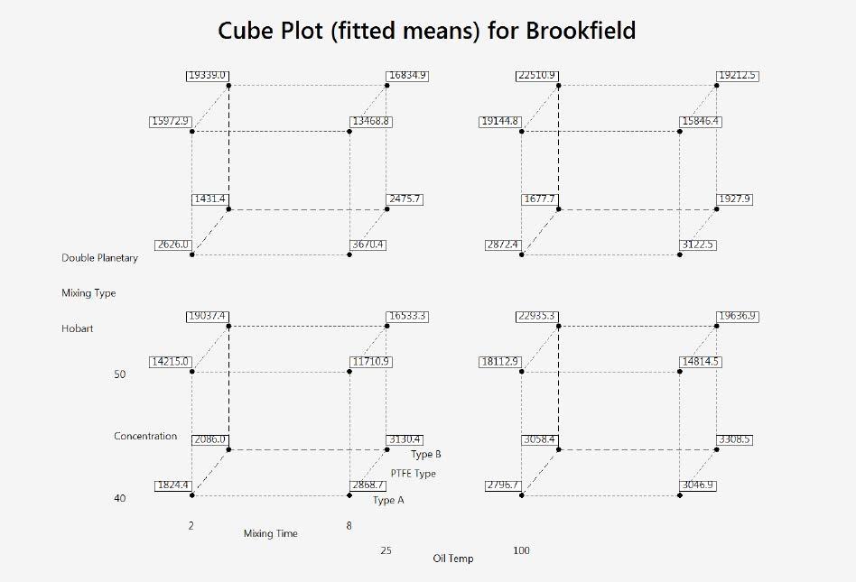
Figure 6: DOE Cube Plot with Fitted Means

Figure 7: Pareto Chart of the Standardized Effects

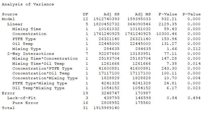
Through analysis of the ANOVA results in Table 1 from the DOE and as shown in the Pareto chart in Figure 7, it is apparent that all the main factors except mixing type were significant. The DOE also discovered several interaction effects.

The correlation between PTFE type and concentration was expected based on historical experience with the material. The two grades of PTFE chosen for this work had slightly different thickening efficiencies, probably related to the primary particle size and the surface area of the PTFE particles. The interaction effect between mixing time and concentration has illustrated the need to modulate the amount of mixing time based on the amount of PTFE thickener used and the final apparent viscosity to maximize the thickening efficiency. While this could have been an apparent assumption, this study proved this to be a statistically significant factor in the manufacturing of a lubricating grease. As the oil temperature for PTFE addition increased, the PTFE thickening efficiency also increased, which in turn lowered the concentration required to meet the Brookfield apparent viscosity requirement. The possible reasons behind this are 1) the thinning of the oil at higher temperature allows it to wet out the surface of the PTFE particles better; or 2) the heat deforms the PTFE and allows for better mechanical mixing of the oil and thickener. This is a very important factor because base oil temperature can vary during the manufacturing of a grease depending on production schedules an season of the year. The type of mixing was not always significant by itself, but it sometimes had a significant interaction effect that depended on the PTFE type. With Type B PTFE, the type of mixing did not matter, but for Type A PTFE, the extra shear provided by the dual planetary mixer made a significant difference at given concentration level and mixing time. The mixing type also had an interaction effect with the amount of PTFE used in the formula. While both styles of mixing can accomplish the end goal, one style will be more efficient above a concentration threshold. This creates an economic trade-off between the cost of mixing time and the ROI of the mixing equipment. Oil temperature also correlated with the mixing time. This led to the hypothesis that there was a three-way interaction between mixing time, PTFE concentration, and oil temperature. Although the interaction of mixing type and oil temperature was significant, it was most likely a consequence of the confounding of mixing time, PTFE type, and PTFE concentration. A further study could be done to investigate further, but that would be beyond the scope of this study. Since both factors will be controlled in the optimization, this will be assumed to be based on confounding.

The residuals from the 25-1 half-fractional DOE are displayed in Figures 8, 9, and 10. The residuals are normally distributed and evenly spaced. There are two residuals that are slightly higher outliers on either end. These two runs represent maximums of the response and were verified through additional repeated runs for validation. When the residuals were tested with the Anderson Darling test [9], it confirmed the normality. This shows how well the model represents the data and the amount of error. From these results, the data models 99.5% of the variation in the process. Based on this and the normal distribution, there was very little error (true or random).

In the residuals versus fit plot, Figure 9, there is a vertical line of residuals that could represent a possible error in the experiments. These points were the measurements of greases prepared with the highest PTFE concentration and blended with the double planetary mixer. This showed a very strong interaction and correlation. The overall random distribution of points around zero illustrates that there was very little random error in this experiment.

The residuals plotted against observation order in Figure 10 are randomly distributed around zero and clearly illustrate that there was no error introduced into the experiment through the order in which the greases were tested. This indicates that the experimental testing plan was properly randomized, and the order of testing had no effect on the results.

Optimization

With an accurate empirical model that represents this experimental process and a region of the design space that is on both edges of the specification, a Central Composite Response Surface DOE Design can be built around it. Since this face had a response on both sides of the specification, the goal is to move the response towards the Optimum Region. There were many significant factors in the full DOE. To save costs and time for this Response Surface Methodology (RSM) DOE, the model is reduced where it makes the most sense and where trade-offs are acceptable.

Before the RSM model was constructed, a computational optimization was performed to aid in the prediction and setting of model parameters. This optimization methodology was a multi-objective genetic algorithm. Through the analysis of the 25 Half Fractional DOE, a regression equation was created. This objective function was used to optimize the apparent viscosity (f) and was combined with a second objective function which was created to minimize the cost of the product. The objective functions and constraints are on the next page. Figure 8: Normal Residual Plot

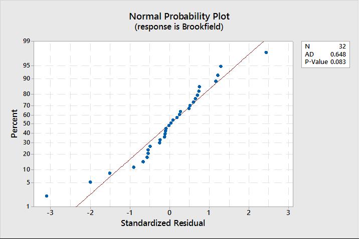
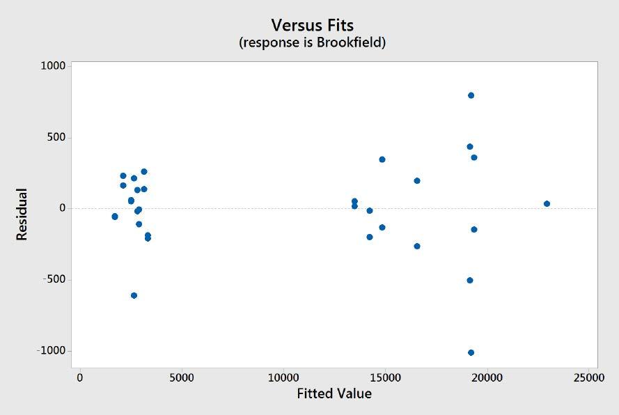
Figure 9: Residual Plot Vs. Fit

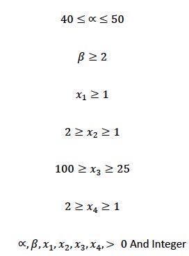
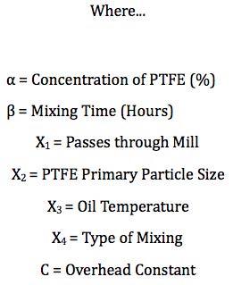
This optimization requires working with two objective functions which had conflicting optimal solutions. This meant that as the apparent viscosity was maximized, the optimal solution for cost degraded. To solve this optimization problem, the Genetic Evolutionary Multi-Objective Optimization technique was used [4]. Since this evolutionary algorithm is a partial stochastic search method for determining the optima on the Pareto Frontier, multiple runs were made to validate the results. The solutions produced from this optimization algorithm did not guarantee an optimal solution as tradeoffs would be needed to satisfy both objective functions.

The Multi-Objective Genetic Evolutionary method used in this optimization was set up in the following manner. The initial populations were tested using minimums, maximums, and a random starting point. The selection process for choosing parents for the next generation was based on a tournament function, which chooses individuals for the mating pool at random and then selects the best individual out of that set to be a parent. Children for the next generation are created 99% by a crossover function and 1% by mutation. The mutation of a child in the next generation is governed by a Gaussian function where the random number used to decide whether to mutate or not is from a Gaussian distribution.

The multilobe function that was used in Matlab utilizes a controlled elitist genetic algorithm (variant of NSGA-II [4]). This type of genetic algorithm always favors individuals with a better fitness value (rank) to the objective function. This type of genetic algorithm also favors individuals that increase the population diversity even with a lower fitness value. The diversity of a population is important to maintain a convergence to an optimal Pareto Frontier. The diversity of the population is maintained by controlling the elite members of the population as the algorithm progresses. This is controlled by two functions (ParetoFraction and DistanceCrowding) which control the elitism through diversity. The ParetoFraction function limits the number of individuals which are elite members on the Pareto Frontier, as domination by pure elite members of the population may lead to solutions that are not optimal or less optimal in the Pareto Frontier. The distancing function helps to maintain diversity on the Pareto Frontier by favoring individuals that are relatively far away on the Frontier. This algorithm stops the optimization run if the spread, which is a measure of the spacing distance on the Pareto Frontier, becomes smaller than the stopping tolerance. The migration of individuals that could be strong candidates was checked in both direction of sub-populations, meaning that the nth subpopulation migrates into both the (n −1)th and the (n +1)th sub-populations. This helps ensure that all possible solutions are covered in the optimization method.

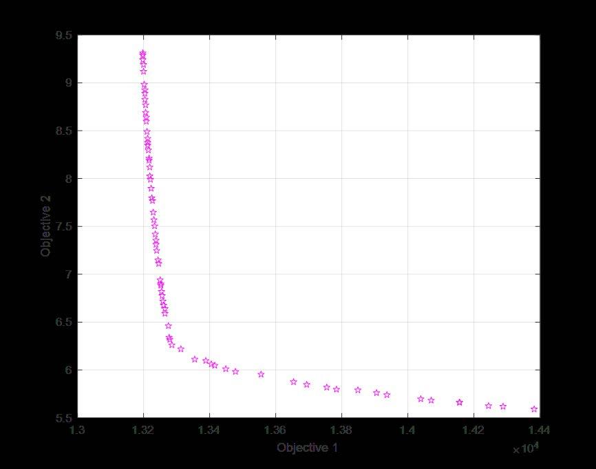
In Figure 11, the Pareto Frontier for the two objective functions is shown. The Pareto Frontier represents a series of optima that exist in the feasible design objective space. The Pareto Frontier plot has one objective function plotted on each axis and a curve which represents all the feasible Pareto Solutions or optima which satisfy both objective functions.

The two objective functions were evaluated 10 times each using the Genetic Evolution method with four different starting points to look for statistically significant differences. With a 95% confidence interval, it was found that all evaluations had no statistical difference between groups or within the different groups.

Because of the DOE, boundary constraints were found for manufacturing this product with high repeatability. This also helped create the framework for the optimization work in this project. To maximize the main controlling factor of the PAO-PTFE grease (Brookfield Apparent Viscosity), we would originally end up moving towards the upper anchor point on the Pareto Frontier as cost increases greatly.

Through use of the genetic evolution algorithm, a set of conditions was found for each of the control variables that satisfied both objective functions. However, as it is impossible to optimize two objective functions simultaneously, some trade-offs must be made. These trade-offs will be made to balance the main performance characteristics of the PAOPTFE grease and the objective function for cost.

Through the computational optimization, it was determined that this product can be designed to meet the solutions found on the Pareto Frontier after making some trade-offs. After doing a trade-off analysis, it was determined that the target values would be 47.5% PTFE (Type B), 10 hours of mixing at a temperature of 63 to 86⁰C The mixing style was not significant, although it did have a stronger effect on the Type A PTFE,

Figure 11: Pareto Frontier Plot for Computational Optimization

which illustrates that either mixing style can be utilized. The RSM design will move forward with the double planetary mixing system and the Type B PTFE based on its relative cost and because the DOE showed it to be more efficient in thickening efficiency. All other non-variable factors will continue to be controlled.

The final two factors, the variables for the RSM design, are PTFE content and mixing time. The response surface design will be a full factorial central composite design (CCD) with these two continuous factors. This design will have four cube points, seven total center points (three in the cube, four axial), and four axial points. The alpha value for the design will be 1.41421 which was calculated for this design to ensure orthogonality and rotatability. By making the response surface design rotatable, all points will be equidistant from the design center giving them the same prediction variance. The limits for the DOE will be built around the axial points with the mixing time being a low of 4 hours and a high of 12 hours and the concentration of PTFE having a low of 45% and a high of 50%. This places the centroid point at 8 hours and 47.5% and the cube points spaced around this based on the alpha value.

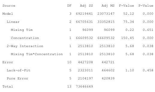
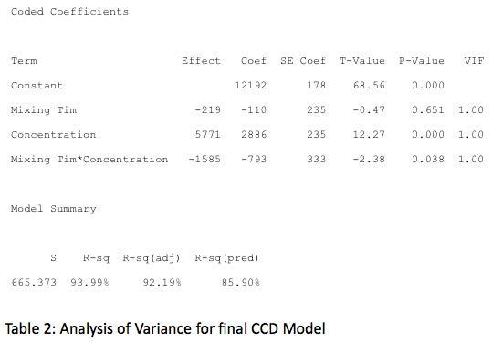
The ANOVA analysis of the results for the response surface design showed that the only terms of statistical significance were concentration and the two-way interaction of concentration and mixing time. There were no quadratic effects in this model. As the quadratic terms were insignificant, the model was reduced by removing the mixing2, concentration2, and the block terms in the model, one at a time.

The variance inflation factor (VIF), which describes the severity of multicollinearity, shows that there is virtually no correlation between the terms of the model. It also indicates that the model is orthogonal, as the VIF is around 1. The residuals from the DOE, as seen in Figure 12, are normally distributed with no outliers. This represents how well the model represents the data and the amount of error. From these results, the coefficient of determination R2 shows that the model accounted for 93.99% of the variation in the data. Based on this result and the normal distribution, there is very little error (true or random).

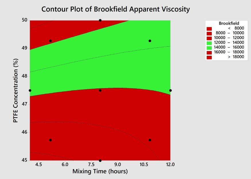
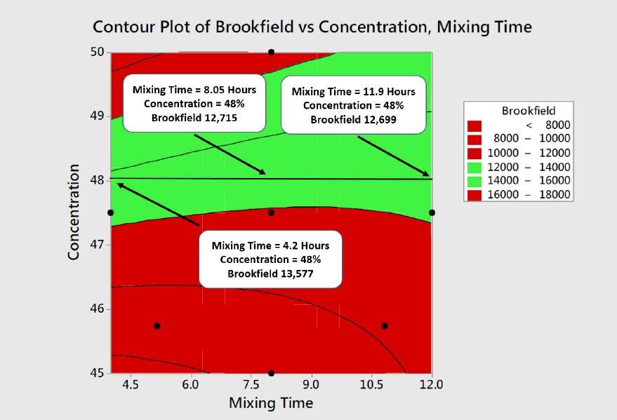
In Figures 13 and 14, the Brookfield response is plotted on a contour plot. All the design points have been included for the cube, center, and axial points to help visualize the design space. In Figure 13, the contours have been colored based on the performance goals for the product, with red and green representing material that is outside of and within specification, respectively. As can be seen in this plot, many possible points satisfy the specification, so additional knowledge and factors must be used to select the process conditions. In Figure 13, data tags were added along the 48% concentration line. The 48% concentration level was chosen to ensure a robust solution and minimize cost. At this concentration level, a mixing time of 4 to 8 hours produced an apparent viscosity that stabilized around 12,700 Poise (P). Additional testing was done with a 48% concentration and 24 hours of mixing; this result fell within this stabilized range. Figure 12: Normal Probability Plot for RSM Optimization

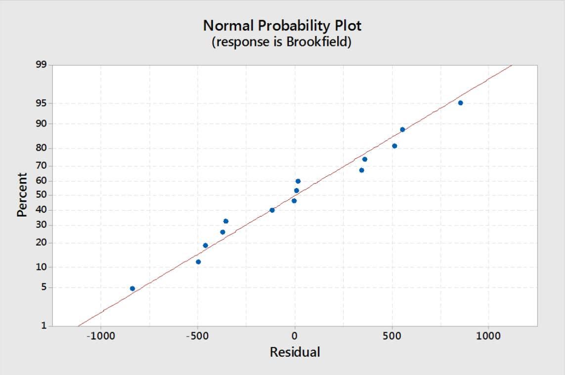
Figure 13: RSM Optimization Contour Plot of Apparent Viscosity

The use of design of experiments (DOE) methodology in this work has allowed for a product to be designed and optimized in a manner that reduces the amount of time needed as well as the development cost. In Table 3, this Planned DOE is compared to several “One at a Time” experimental development projects of similar complexity. In this Table, various times associated with development are compared as well as a normalized time for the project and a total development timeline. It is also important to note that in traditional trial-and-error approaches, it is very easy to miss important factors and interactions that can be misleading and lead to future problems that entail additional development and scale-up costs.

Results from this DOE and optimization of a new PAO-PTFE lubricating grease show that it is feasible to reduce the variation in the process which allows for a more robust product design. The DOE provided critical knowledge regarding this product design and gave solid evidence about interactions during the manufacturing process of the lubricant. The empirical formula developed in this study allowed for a computational optimization that was a very good approximation of the response surface optimization. This is an area where additional time and expense can be saved with confidence (high R2) in the future using the empirical formula and optimization.

The Box-Behnken experiment illustrated the interactions of various factors in the wear testing and how kinematic viscosity and the additive concentration affected the wear produced by the lubricant. Through understanding these relationships between test conditions, viscosity, and the additive, it was possible to predict the wear based on the conditions of the end-use application. This deeper understanding of how and why the lubricant performs made it easier to target a formulation to solve the tribological problem based on statistical data.

The use of statistical analysis and design of experiments methodology may be considered time-consuming and expensive. Through this study, it has become apparent that the development of a new product through DOE optimization methods can be far more efficient in time and cost than “one at a time” experiments. The success of this approach depends on the expertise of staff that understand the raw materials and project goals to develop appropriate statistical models.

It has been many years since the term “tribology” was coined following the Jost report [10]. The focus in the industry is centered around reducing friction and conserving energy. The use of DOE methodologies is a step forward on that path, as it can help conserve time and energy expended to development products and optimize them to meet real world needs.

Table 3: Time Comparison of DOE and “One at a Time” Experiments

Acknowledgments

I would like to thank my colleagues in the Research and Development Lab at Nye Lubricants Inc. who made and tested the samples for this work. I would also like to thank Dr. Wenzhen Huang from the University of Massachusetts at Dartmouth for his support and guidance.

DOE Appendix

Design of Experiments Methodology - Details

The use of regression analysis and Analysis of Variance (ANOVA) are critical statistical tools used in the analysis of a DOE experiment. There are many types of DOE models including factorial, central composite, Box-Behnken, D-Optimal, and Taguchi. In Figure A1, the different types of DOE models are illustrated in a three-dimensional geometry where the cube represents the experimental design region.

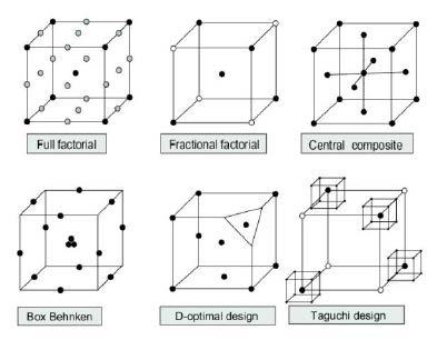
Figure A1: DOE Models

Before a DOE is undertaken, other tools like a fishbone (Ishikawa) diagram are used to specify expected causes of variation in a process or product. This would typically be created by a team comprised of stakeholders and subject matter experts (SME) in a brainstorming session where the goal is to identify the important factors and levels to be tested in the experiment. In an experiment, levels can be considered as the boundaries for a process or design region.

Some keys to the success of a DOE is accurate data collection, control of all possible variables, and randomization. If an experimental design is randomized, the bias effects in the response can be reduced or eliminated. The control of variables is critical to a good experiment as the error will increase significantly without control. Sometimes this will happen as one variable will be considered non-significant by the team or hard to control (HTC).

A good example of this is the oil temperature when an additive is combined with the oil. In this study, the additive was added to oil at 100⁰C in some cases, while other times it was added to oil at ambient temperature. This temperature factor was not included in the initial DOE study however when the results were analyzed, there was unexplained variance in the results. After performing the experiment again and taking this variable into consideration, the temperature at which this additive was added to the oil was found to be a significant factor and to have interaction effects on mixing time, processing time, and other factors.

The above example illustrates some keys to success and possible pitfalls of ignoring significant factors. Even in a case where a factor itself may not be highly significant on its own, it may have strong interaction effects that reduce the accuracy of the DOE. It is critical that all the experimental conditions are as controlled and accurate as possible.

The simplest of these DOE models is the general factorial design. These experiments consist of 2 or more variables that have at least two levels for each variable. In a full factorial experiment, all levels for all variables are studied, which allows the experimenter to learn about each independent variable and its effect on the response as well as interactions with other variables. This works well for small or well-defined experiments, but in cases where there are many factors or levels, a fractional factorial design is used.

Fractional factorial models use half or a quarter of the test points and estimate the remainder through statistical methods.

The central composite design (CCD) [7] as shown in

Figure A2 expands upon the factorial model by adding center and axial points and is a typical method used to fit a second order response surface. The axial points are test points that are found outside of the full factorial design surface and are spaced equally away from the center-point by α. The α value is designed to ensure orthogonality and rotatability of the design and by making the design rotatable, all points will be equidistant from the design center giving them the same prediction variance. Ensuring that the design is orthogonal allows for individual effects to be estimated independently with minimal confounding as well as making sure the model coefficient is uncorrelated.

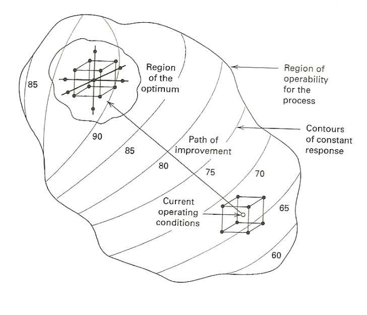
The central composite design is normally applied with a response surface methodology (RSM) for a sequence of designed experiments to obtain an optimal response from a system or process. When using RSM, it is normal to first run a factorial DOE and once an area of improvement has been found, a numerical optimization method like steepest descent (or ascent) can be used to find the region of the optimum (See Figure A3.). Once in the optimum design region, a RSM experiment can be performed to find the response surface around an optimum point which will tell you how the system response responds to changes in the variables. This is typically seen as curvature in the response which represents finding the contours of a design and moving from an optimum value to one of degrading performance.

Figure A2: Two and Three Factor Central Composite Design

Figure A3: RSM Design Methodology

The Box-Behnken [8] [9] experimental design is a type of response surface design but with a major difference that it does not contain an embedded factorial design. This design is normally chosen when all the test points needed for the experiment must be contained within the design space and axial points are not feasible. Since all the test points fall within the design space, they will be combinations of the high and low levels for the factors and their midpoints. This design will also incorporate center points; however, corner points are not evaluated as this design operates under the assumption that the corner points (the extremes of all factor levels) rarely occur together and are not evaluated directly. This allows fewer experimental runs as the data for the corner points are estimated. This design also allows good estimation of main factor effects and second order interactions. Its downside is that it cannot be used for sequential experiments as it lacks the embedded factorial design.

References

1. Dirk Gorissen, Ivo Couckuyt, Piet Demeester, Tom

Dhaene, and Karel Crombecq. A surrogate modeling and adaptive sampling toolbox for computer based design.

Journal of Machine Learning Research, 11(Jul):2051 2055, 2010.

2. Nestor V Queipo, Raphael T Haftka, Wei Shyy, Tushar

Goel, Rajkumar Vaidyanathan, and P Kevin Tucker.

Surrogate-based analysis and optimization. Progress in aerospace sciences, 41(1):1 28, 2005.

3. Douglas C Montgomery, Elizabeth A Peck, and G Geoffrey

Vining. Introduction to linear regression analysis. John

Wiley & Sons, 2015.

4. Kalyanmoy Deb, Samir Agrawal, Amrit Pratap, and Tanaka

Meyarivan. A fast elitist non-dominated sorting genetic algorithm for multi-objective optimization: Nsga-ii.

In International Conference on Parallel Problem Solving from Nature, pages 849 858. Springer, 2000.

5. Box, George EP, William Gordon Hunter, and J. Stuart

Hunter. Statistics for experimenters: an introduction to design, data analysis, and model building. Vol. 1. New

York: Wiley, 1978. 6. Pettitt, A. N. "Testing the normality of several independent samples using the Anderson-Darling statistic." Applied

Statistics (1977): 156-161.

7. Raymond H Myers, Douglas C Montgomery, G Geo rey

Vining, Connie M Borror, and Scott M Kowalski. Response surface methodology. Journal of Quality Technology, 36(1):53 78, 2004.

8. George EP Box and Donald W Behnken. Some new three level designs for the study of quantitative variables.

Technometrics, 2(4):455 475, 1960.

9. Raymond H Myers and Douglas C Montgomery. Response surface methodology: Process and product in optimization using designed experiments. 1995.

10. Jost, H. Peter. Lubrication: Tribology; Education and

Research; Report on the Present Position and Industry's

Needs (submitted to the Department of Education and

Science by the Lubrication Engineering and Research)

Working Group. HM Stationery Office, 1966.