Essay: The Forsaken Victims of Climate Change

Lastly, climate change multiplies the number of health issues that exist in poorer regions. A warmer climate means warmer freshwater sources, which in turn provide a more habitable place for harmful bacteria and microbes to grow. The World Health Organization (WHO) estimates that 3.575 million people die from water-related diseases per year, and with increased temperatures drying out available water sources, people driven desperate by thirst are forced to choose between the risks of drinking contaminated water or dying of thirst. Additionally, the increased smog caused by warmer atmospheres, coupled with severe air pollution, has made it impossible to breathe in places such as Delhi, where the quality of air reached such high toxicity that experts deemed it equivalent to smoking 50 cigarettes a day (Paddison, 2020). In fact, the WHO claims that over 90% of the world population breathe in some form of toxic air, leading to an abundance of diseases like stroke and lung cancer (Fleming, 2018). Even within the U.S., poorer communities in both rural and urban areas bear the greatest burden of climate change, as seen by lack of health insurance, dependence on agriculture-based economies, and no funds to recover from natural disasters. In urban areas, which produce 80% of greenhouse gas emissions in North America, the poor live in neighborhoods with the greatest exposure to climate and extreme weather events (Chappell, 2018). Poorer Americans, while to a much lesser extent, face some of the same disadvantages as those living in developing countries in terms of environmental inequality. So what exactly is being done to save our planet and its poorest inhabitants?

One thing is for sure: not enough. The overall global response to climate change can be characterized as extremely uneven. Persistent skepticism from certain global leaders, many of whom are motivated by economic interests, is slowing cooperative efforts to address the issue of climate change. In particular, President Trump’s decision to withdraw from the Paris climate agreement will trigger both short-term and long-term damage—for one, it will be less likely for the U.S., the second-highest ranking country in production of greenhouse gases, to reduce carbon emissions without international obligations, and countries that were already hesitant about membership are more likely to back off as well (“The Uneven Global Response to Climate Change,” 2019). President Trump's decision in times like these is brutal, as the urgency of action is greater now than ever before, as indicated by the World Meteorological Organization’s 2019 report. The report showed a continued increase in greenhouse gases to new records during the period of 2015-2019, with CO2 growth rates nearly 20% higher than the previous five years (“Global Climate in 2015-2019,” 2019). Surrounded by a constant whirlwind of bad news, it can feel like all hope is lost for planet Earth.

But hope is not lost. The global effort to address climate change is moving forward as a whole, even without the current support of the U.S. government. Plenty of countries are setting goals to reduce emissions and implement renewable energy. Morocco has invested heavily in solar power, and India has implemented a prohibition of new coal plants (“The Uneven Global Response to Climate Change,” 2019). China, the world’s number one CO2 contributor at a whopping 29% of global emissions, has made great strides in reducing air pollution (“Each Country's Share of CO2 Emissions,” 2019). The youth movement across multiple nations, led by activist Greta Thunberg, is on the rise, and hundreds of new green technologies are making their way towards the market. The most promising of these innovations include solar cells that incorporate the mineral perovskite, which convert UV and visible light with a stunning 28% efficiency (as compared to the average 15-20%), graphenebased batteries that power electric vehicles, and carbon capture and storage that traps CO2 at its source and isolates it underground (Purdue University, 2019).

While these global pledges and new technologies hold great promise for future sustainability, it is up to us to actively implement more environmentally conscious decisions into our daily lives. Reduce, reuse, and recycle in that order. Eat a more plant-based diet. Conserve energy at every moment possible. Always be civically engaged. We owe it to not only the animals, our children, and our home; we owe it to those who contribute least to the climate change devastation but feel its effects most deeply. We must not let our privilege go wasted.

References

Chappell, C. (2018, November 27). Climate change in the US will hurt poor people the most, according to a bombshell federal report. Retrieved January 7, 2020, from https://www.cnbc.com/2018/11/26/climate-changewill-hurt-poor-people-the-most-federal-report.html.

Each Country's Share of CO2 Emissions. (2019, October 10). Retrieved January 8, 2020, from https://www.ucsusa. org/resources/each-countrys-share-co2-emissions.

Fleming, S. (2018, October 29). More than 90% of the world's children are breathing toxic air. Retrieved January 9, 2020, from https://www.weforum.org/agenda/2018/10/more-than-90-of-the-world-s-children-arebreathing-toxic-air/.

Giovetti, O. (2019, September 25). How the effects of climate change keep people in poverty. Retrieved January 7, 2020, from https://www.concernusa.org/story/effectsof-climate-change-cycle-of-poverty/.

Global Climate in 2015-2019: Climate change accelerates.

(2019, September 24). Retrieved January 8, 2020, from https://public.wmo.int/en/media/press-release/global-climate-2015-2019-climate-change-accelerates.

Hausfather, Z. (2017, December 13). Analysis: Why scientists think 100% of global warming is due to humans. Retrieved January 8, 2020, from https://www.carbonbrief.org/analysis-why-scientists-think-100-of-globalwarming-is-due-to-humans.

Johnson, S. (2019, November 22). What Are the Primary Heat-Absorbing Gases in the Atmosphere? Retrieved January 7, 2020, from https://sciencing.com/primary-heatabsorbing-gases-atmosphere-8279976.html.

Paddison, L. (2020, January 3). 5 Environmental News Stories To Watch In 2020. Retrieved January 9, 2020, from https://www.huffpost.com/entry/environment-heat-wave-climate-change-elections_n_5def87d7e4b05d1e8a57cb90.

Plumer, B. (2017, April 18). How rich countries "outsource" their CO2 emissions to poorer ones. Retrieved January 9, 2020, from https://www.vox.com/energy-and-environment/2017/4/18/15331040/emissions-outsourcing-carbon-leakage.

Purdue University. (2019, November 12). New material points toward highly efficient solar cells. Retrieved January 9, 2020, from https://www.sciencedaily.com/ releases/2019/11/191112164944.htm.

Schwartz, E. (2019, November 19). Quick facts: How climate change affects people living in poverty. Retrieved January 8, 2020, from https://www.mercycorps.org/articles/climate-change-affects-poverty.

The Causes of Climate Change. (2019, September 30). Retrieved January 7, 2020, from https://climate.nasa.gov/ causes/.

The Uneven Global Response to Climate Change. (2019, November 18). Retrieved January 7, 2020, from https:// www.worldpoliticsreview.com/insights/27929/the-uneven-global-response-to-climate-change.

SMALL MOLECULE ACTIVATION OF WNT/ β-CATENIN SIGNALING PATHWAY ON NEURODEGENERATION RATES OF DOPAMINERGIC NEURONS IN C. ELEGANS

Ariba Huda

Abstract

Parkinson’s Disease (PD) is a neurodegenerative disease characterized by loss of midbrain dopaminergic (mDA) neurons. While there are several medical treatments available for PD, they often come with significant side effects and do not act as definite cures. Past studies have indicated that Wnt/β-Catenin signaling is critical for the generation of dopamine (DA) neurons during development and for further neurorepair. This study investigates the roles of small molecules, Wnt Agonist 1 and Pyrvinium, in Wnt signaling and their effects on neurodegeneration. Wnt signaling was modeled by Caenorhabditis Elegans (C. elegans), nematodes that display dopamine-dependent behavior in response to neurodegeneration. 24 hour exposure to Wnt Agonist 1 has been shown to significantly reduce neurodegeneration as observed through locomotor behavior and chemotaxation. Currently, work is being done to measure BAR-1 and other Wnt related ortholog gene expression within Wnt Agonist 1 exposed worms. Analysis of the functions behind the Wnt/β-Catenin signaling pathway in the generation and neurorepair of mDA neurons will allow further understanding of the potential for PD stem cell therapies.

1. Introduction

1.1 – Parkinson’s Disease

Parkinson’s Disease (PD) is a neurodegenerative disease that results from the progressive cell death of dopaminergic (DA) neurons. Currently, various medications are prescribed to patients to control symptoms such as cognitive decline and loss of motor function, but there is no definitive cure. The most common therapy is the drug levodopa (L-DOPA), which is used to stimulate dopamine production in neurons associated with motor skill. However, while L-DOPA is efficient at managing the extent of symptoms, it also has various side effects on patients, ranging from physiological to psychological. At present, research is being conducted to identify the clinical applications of stem cell therapy in Parkinson’s Disease as well as the genetic factors behind PD [1]. These discoveries could contribute to the development of a new therapy option geared towards reducing the adverse effects of medications on diagnosed patients.

Dopamine neurons are located in the human nigrostriatal pathway, a brain circuit that connects neurons in the substantia nigra pars compacta with the dorsal striatum. Despite lack of a specific cause for neuronal loss, DA neuron loss has been linked to genetic mutations and environmental toxins [2]. Studies have shown that DA neurons have a distinctive phenotype that could contribute to their vulnerability. An example of this is the opening of L-type calcium channels, which results in elevated mitochondrial oxidant stress and susceptibility to toxins [2]. Moreover, DA neurons are susceptible to degeneration because of extensive branching and amounts of energy required to transmit nerve signals along these branches [3].

1.2 – Wnt/β-Catenin Signaling Pathway

Due to the significance of the Wnt signaling pathway for the healthy functioning of the adult brain, dysregulation of these pathways in neurodegenerative disease has become notable. Wnt/β-Catenin signaling is also critical for the generation of DA neurons in embryonic stem cells [4]. Since several of the biological functions disrupted in PD are partially controlled by Wnt signaling pathways, there is potential for therapy centered around targeting these pathways [4].

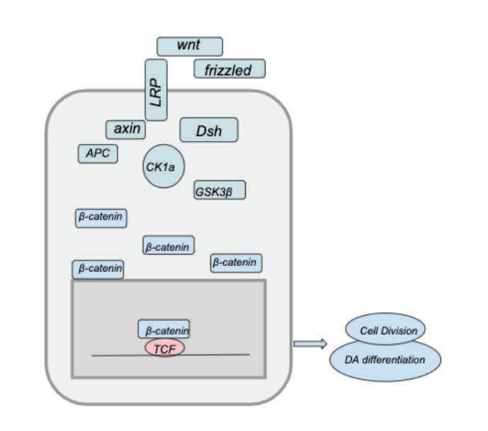
In an activated state, Wnt proteins act as extracellular signaling molecules that activate the Frizzled receptor. Following the activation of Frizzled, the LRP receptor undergoes phosphorylation, inducing the translocation of the destruction complex, a complex of proteins that degrades β-catenin, to the region of membrane near the two receptors (Fig. 1). The activated dishevelled (Dsh) proteins cause the inhibition of the destruction complex which prevents β-catenin phosphorylation. Overall, an activated state of the Wnt/β-Catenin signaling pathway causes an increase in β-Catenin levels.

The transcription factor TCF mediates the genetic action of Wnt signaling patterns, leading to the induction of Wnt targeted genes. When β-Catenin levels increase, they are translocated to the mitochondria, dislodging the Groucho protein from TCF, and binding to TCF leading to the transcription of Wnt targeted genes. The expressed genes regulate cellular growth and proliferation. Without

Wnt stimulation, cytoplasmic β-Catenin levels are kept low through continuous proteasome-mediated degradation.

Figure 1. Activated Wnt Signaling Pathway. Dsh is activated when Wnt binds to the Frizzled receptor. Consequently, the inhibition of the destruction com-

plex leads to increased expression of β-Catenin.

Recent studies have found that the canonical Wnt/β-Catenin pathway is a key mechanism in controlling DA neuron cell fate decision from neural stem cells or progenitors in the ventral midbrain [5]. Wnt acts as a morphogen which activates several signaling pathways, specifically regulating the development and maintenance of midbrain dopaminergic (mDA) neurons [6]. Wnt proteins have also been shown to regulate the steps of the processes DA neuron specification and differentiation (Figure 2). Previous research in mice found that the Wnt/β-Catenin signaling pathway is required to rescue mDA neuron progenitors and promote neurorepair [4].

Figure 2. The development of midbrain dopamine neurons. mDA neurons arise from neural progenitors in the ventral midline, and are divided into 3 separate phases: regional and neuronal specification (phase I), early (phase II), and late differentiation (phase III) [20].

New approaches in stem cell research have utilized developmental molecules to program embryonic stem cells. The key ingredient for this is glycogen synthase kinase (GSK-3β), a protein found in the destruction complex of the Wnt/β-Catenin signaling pathway [7]. The phosphorylation of a protein by GSK-3β inhibits activity of its downstream target. GSK-3β is active in a number of pathways, including cellular proliferation, migration, glucose regulation, and apoptosis.

1.3 – Wnt Agonist 1 and Pyrvinium

The most notable Wnt activators work by inhibiting the GSK-3β enzyme found in the β-Catenin destruction complex [7]. By inhibiting GSK-3β, Wnts disrupt the ability of the complex to degrade β-Catenin, allowing β-Catenin to accumulate in the nucleus and relay the Wnt signal for transcription. Further, it has been shown that GSK-3β dysregulation contributes to PD-like pathophysiology and accumulation of alpha-synuclein [7]. Wnt Agonist 1 (Fig. 3) is a cell-permeable, small molecule agonist of the Wnt signaling pathway. Wnt Agonist 1 induces accumulation of β-Catenin by increasing TCF transcriptional activity and altering embryonic development [8]. Studies have found that the stimulation of Wnt/β-Catenin signaling pathway with the Wnt agonist has been able to reduce organ injury after hemorrhagic shock [9].

Figure 3. Wnt Agonist 1 Structure, (C H ClN O ). A 19 19 4 3 crystalline solid. Formula weight: 350.4

Pyrvinium (Fig. 4) has been found to be a small molecule inhibitor of the Wnt signaling pathway through activation of casein kinase 1a [10]. In most eukaryotic cell types, the casein kinase 1 family of protein kinases are enzymes that function as regulators of signal transduction pathways. Studies have demonstrated that pyrvinium binds to and activates CK1α, a part of the β-Catenin destruction complex. CK1α members play a critical role in Wnt/β-Catenin signaling, acting as both a Wnt activator and Wnt inhibitor [10].

Clinical research in neurodegenerative diseases has not been done with Wnt Agonist 1 and Pyrvinium. However, Wnt Agonist 1 has been shown to be effective in vivo, de-

creasing tissue damage in rats with ischemia-reperfusion injury [21]. Pyrvinium salts have been shown to inhibit the growth of cancer cells [10]. Additionally, Pyrvinium has been shown to be an effective anthelmintic, a drug used to treat infections of animals with parasitic worms [22].

Figure 4. Pyrvinium Structure, (C26H28N3+). Formula Weight: 382.53

1.4 – C. Elegans Model

C. elegans is a popular model for neurodegenerative research. The transparency of C. elegans makes it easy to facilitate the study of specific neurons and genetic manipulation [11]. C. elegans also present locomotor behavioral responses to neurodegeneration. The identification of genes that cause monogenic forms of PD allows for easy modeling in C. elegans. Studying a C. elegans model of PD can provide insight into the cellular and molecular pathways involved in human disease. C. elegans are also able to be used to identify disease markers and test potential treatments. Outcome measures are used to detect disease modifiers such as survival of dopamine neurons, dopamine dependent behaviors, mitochondrial morphology and function, and resistance to stress. Behavioral markers studied in C. elegans to detect PD include basal slowing, ethanol preference, area restricted searching, swimming induced paralysis, and accumulation of α-synuclein [12]. Dopamine neuron location sites are present within hermaphroditic and male specific worms (Fig. 5). This project will further investigate the role of C. elegans in neurodegenerative research in place of previously used vertebrate models.

1.5 – Hypothesis

Due to the significant role Wnt/β-Catenin signaling plays for DA neuron differentiation in development, activated signaling within worms will decrease neurodegeneration rates. Thus, if worms are exposed to increasing concentrations of Wnt Agonist 1, they will display lower rates of neurodegeneration due to activated Wnt/β-Catenin signaling and increased β-Catenin expression. On the other hand, if worms are exposed to increasing concentrations of Pyrvinium, they will display higher rates of neurodegeneration due to CK1α activation and inhibited Wnt/β-Catenin signaling. Furthermore, if worms are exposed to respective treatments during development, their neurodegeneration rates will increase or decrease more drastically compared to adult worms who are not exposed to any treatment.

Figure 5. Top represents a hermaphrodite C. elegans and bottom represents a male C. elegans with their respective DA neuron sites. R&L stands for right and left side. CEPD neurons are mechanosensory neurons. ADE neurons are anterior deirid neurons. PDE neurons are post embryonically born posterior deirid neurons. All neurons have DOP-2 dopamine receptor. R5a, R7a, and R9a neurons are male specific sensory ray neurons [25].

2. Methods

This study consists of a preliminary experiment, two main experiments, and a secondary experiment. The two C. elegans strains used in this project were the OW13 and N2 type worms. OW13 overexpressed alpha-synuclein and displayed PD-like symptoms. N2 worms acted as the control group, representing wildtypes with no genetic alterations. The same treatments were administered to both worms for each of the following experiments. Treatments administered included three separate concentrations of Wnt Agonist 1 and Pyrvinium, as well as dimethyl sulfoxide (DMSO).

2.1 – C. elegans Maintenance

N2 and OW13 strains were purchased from the Caenorhabditis Genetics Center (CGC) at the University of Minnesota. The CGC is funded by the National Institute of Health (P40 OD010440). Worms were placed on nematode growth media (NGM) plates that were spotted with approximately 30μl solution of LB Broth and OP50, a strain of E. coli in the C. elegans diet. Worms were placed onto new plates approximately every 48-72 hours. C. elegans maintenance protocols were followed through WormBook [13].

2.2 – Preparation

Wnt Agonist 1 Preparation: Stock Wnt Agonist 1 was purchased from Selleckchem. 1mg Wnt Agonist 1 was dissolved into 2.5851 mL, 0.5170 mL, and 0.2585 mL DMSO for 1 mM, 5mM, and 10 mM concentrations, respectively. Dilutions were stored in 4oC.

Pyrvinium Preparation: Stock Pyrvinium was purchased from Selleckchem. 1 mg Pyrvinium was dissolved into 0.8685 mL, 0.1737 mL, and 0.0896 mL DMSO for 1 mM, 5 mM, and 10 mM concentrations, respectively. Dilutions were stored in 4oC.

2.3 – Preparation: Experimental Design

Activating Wnt Signaling: During each trial, 6 NGM plates spread with different concentrations of treatment were prepared for each strain of worm. L4 stages of each strain (OW13 and N2) were exposed to three different concentrations (1 mM, 5 mM, and 10 mM) of Wnt Agonist 1. Worms were kept on the plate for approximately 24 hours until they reached the adult stage. Then, approximately half of the worms were transferred to perform the thrashing assays and the remaining worms remained on the plate until the next generation of worms were apparent.

Inhibiting Wnt Signaling: During each trial, 6 NGM plates, spread with different concentrations of treatment, were prepared for each strain of worm. L4 stages of each strain (OW13 and N2) was exposed to three different concentrations (1 mM, 5 mM, and 10 mM) of Pyrvinium. Worms were kept on the plate for approximately 24 hours until they reached the adult stage. Then, some worms were transferred to perform the thrashing assays, and the rest of the worms remained on the plate until the next generation of worms were apparent.

Thrashing Assay: Agar Pads were prepared and approximately 30 worms were picked onto each pad. A drop of M9 buffer was then added. Five minutes after transfer, the number of body bends in 20s intervals was sequentially filmed then counted for each of the worms on the assay plate. This was done after 24 hour exposure to treatment and when the next generation of worms (born to exposure) had reached adult stage. Trials were run 3 times for each treatment group and values were averaged.

2.4 – Statistical Measurements

Averages of locomotor behavior and chemotaxation were calculated and recorded after experimentation. Data were analyzed using unpaired Student t-tests with unequal variance. This is due to differences in sample size per treatment group. Error bars were calculated using standard error of the mean (SEM). 3.1 – Preliminary Data

To determine that OW13 and N2 strains displayed significant differences in neurodegeneration, a preliminary thrashing assay was conducted on OW13 and N2 worms with exposure only to DMSO. These worms represented a non-treatment group. A single thrash is a complete body bend (Fig. 6).

Figure 6. Single thrash (body bend) within 20 second interval. Movement follows from top to bottom.

We can conclude that the number of body bends per 20 second interval is an appropriate measure of neurodegeneration and displays statistically significant differences between N2 and OW13 strains of worms. OW13 worms thrashed at a rate of 34.58 bends per 20 second interval and N2 worms thrashed at a rate of 23.42 bends per 20 second interval (Fig. 7). The OW13 worms with overexpressed α-synuclein showed a significant increase in thrashing in comparison to the wildtype N2 worms. Overexpression of α-synuclein is the main marker of dopamine deficiency and Parkinson’s Disease. This demonstrates that higher rates of thrashing correlate to higher levels of dopamine deficiency within the OW13 strain.

Figure 7. No treatment thrashing score analysis: the number of body bends per 20 second interval were counted for 30 worms per each strain. Then the values were averaged and graphed above. N2 worms moved at an average of 23.42 body bends per interval, with a standard deviation of 3.86, median of 23.5, and standard error of the mean (SEM) of 0.79. OW13 worms moved at an average of 34.58 body bends per interval, with a standard deviation of 4.44, median of 35, and SEM of 0.811. Significance (p<0.05 = *) is represented through bold connecting lines. This shows that worms with Parkinson’s Disease (OW13) move at a faster rate than wildtype (N2) worms. Error bars ± SEM.

4. Main Results

After determining the effectiveness of the analysis of thrashing scores in measuring neurodegeneration, worms were exposed to their own respective treatments (Tab. 1). These treatments were either Wnt Agonist 1 (1 mM, 5mM, or 10 mM concentration), Pyrvinium (1 mM, 5mM, or 10mM concentration), or DMSO. The number of body bends per 20 second interval were counted for 30 worms per each strain and concentration. The values were averaged and graphed below.

Table 1. Organization of worm groups and treatments administered. (Key: 1 = 1mM treatment, 5 = 5mM treatment, 10 = 10mM treatment) Wnt Agonist 1 Effect on DMSO Cancer (Control) OW13 A1, A5, A10 C1, C5, 3 plates of C10 worms exposed to equal concentration

N2 B1, B5, B10 D1, D5, D10 3 plates of worms exposed to equal concentration

Exposure to Wnt Agonist 1 significantly decreased thrashing rates in comparison to the control DMSO worms (Fig. 8). However, this does not show the effect was con- centration dependent. Exposure to Pyrvinium at 5mM and 10mM concentrations killed the worms. 1mM Pyrvinium exposure also resulted in a significant decrease in thrashing rates. In the N2 groups, there is no significant difference between the treatment groups and the control N2 group. Pyrvinium decreased thrashing in relation to the 10mM Wnt Agonist 1 exposure, contradicting the original hypothesis.

Next generation adult worms were collected on the same treatment plates after approximately 5 days. This study further aimed to observe any developmental significance in activated Wnt/β-Catenin signaling within genetically predisposed offspring.

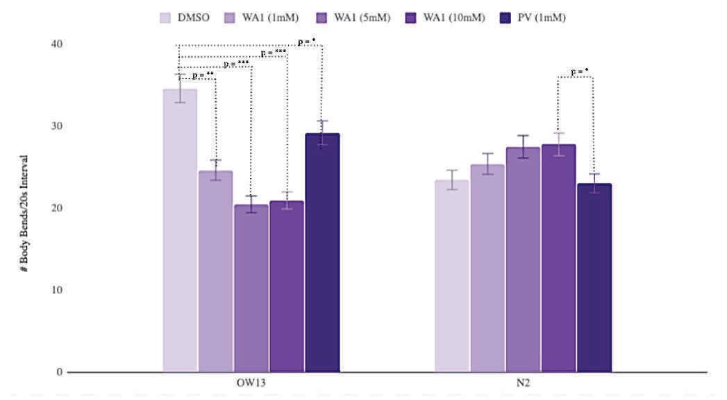
Figure 8. Thrashing score analysis across various treatments after 24 hour exposure: 10 different treatment groups of 30 worms were measured: OW13 Wnt Agonist 1 (1mM) (μ = 24.615 , ̃x = 25, SEM= 0.475); OW13 Wnt Agonist 1 (5mM) (μ = 20.625 , ̃x = 21, SEM= 0.739); OW13 Wnt Agonist 1 (10mM) (μ = 20.923 , ̃x = 21, SEM= 0.630); OW13 Pyrvinium (1mM) (μ = 29.167, ̃x = 29, SEM= 0.632); N2 Wnt Agonist 1 (1mM) (μ = 25.375 , ̃x = 25, SEM= 0.789); N2 Wnt Agonist 1 (5mM) (μ = 27.846 , ̃x = 28, SEM= 0.414); N2 Wnt Agonist 1 (10mM) (μ = 27.75 , ̃x = 28.5, SEM= 0.567); N2 Pyrvinium (1mM) (μ = 23 , ̃x = 23.5, SEM= 0.833); OW13 DMSO (μ = 34.58 , ̃x = 35, SEM= 0.811); N2 DMSO (μ = 23.42 , ̃x = 23.5, SEM= 0.705). Significance (p<0.05 = *, p<0.01 = **, p<0.001 = ***) is represented through dotted connecting lines. Error bars ± SEM.

Similar to the adult worms (Fig. 8), exposure to Wnt Agonist 1 significantly decreased thrashing rates in comparison to the control DMSO next generation worms (Fig. 9). However, there is no significance supporting a concentration dependent effect. Exposure to Pyrvinium at 5mM and 10mM concentrations killed the worms and 1mM Pyrvinium exposure also resulted in significant decrease in thrashing rates. In the N2 groups, there is no strong significance between the treatment groups and the control N2 group. Pyrvinium decreased thrashing in relation to the

10mM Wnt Agonist 1 exposure. The Pyrvinium results might be related to the dual function Pyrvinium has in both activating and inhibiting Wnt signaling.

Figure 9. Thrashing score analysis across various treatments of next generation worms, born into treatment exposure: 10 different treatment groups of 30 worms were measured: OW13 Wnt Agonist 1 (1mM) (μ = 20.929 , ̃x = 21, SEM= 0.793); OW13 Wnt Agonist 1 (5mM) (μ = 20.438 , ̃x = 20, SEM= 0.653); OW13 Wnt Agonist 1 (10mM) (μ = 24.333 , ̃x = 21, SEM= 0.328); OW13 Pyrvinium (1mM) (μ = 22.769 , ̃x = 22, SEM= 0.553); N2 Wnt Agonist 1 (1mM) (μ = 21.75 , ̃x = 25, SEM= 0.405); N2 Wnt Agonist 1 (5mM) (μ = 21.25 , ̃x = 21, SEM= 0.603); N2 Wnt Agonist 1 (10mM) (μ = 25.2 , ̃x = 25, SEM= 0.618); N2 Pyrvinium (1mM) (μ = 26.5 , ̃x = 236.5, SEM= 0.496); OW13 DMSO (μ = 34.58 , ̃x = 35, SEM= 0.811); N2 DMSO (μ = 23.42 , ̃x = 23.5, SEM= 0.705). Significance (p<0.05 = *, p<0.01 = **, p<0.001 = ***) is represented through dotted connecting lines. Error bars ± SEM.

Using the above data, adult thrashing scores and next generation thrashing scores were compared per strain.

Figure 10: Adult versus next generation worm thrashing score analysis: Data collected in both Figure 10 and 11 were replotted adjacent to each other in order for comparison between adult and next generation worms of each strain. Significance (p<0.05 = *, p>0.05 = ns) is represented through dotted connecting lines. Error bars ± SEM.

The thrashing differences between adult and next generation worms exposed to 1mM Wnt Agonist 1, 5mM Wnt Agonist 1, and 1mM Pyrvinium were significant (Fig. 10). Next generation OW13 worms thrashed less when exposed to 1 mM Wnt Agonist 1 and more when exposed to 5 mM Wnt Agonist 1, but less for both in N2 strains. These inconsistent results lead us to conclude that there is no overall significant difference or correlation between adult worms exposed to treatments and their offspring.

5. Discussion

5.1 – Wnt/β-Catenin Signaling Activation on Neurodegenerative Rates

Previous research has shown that Wnt/β-Catenin signaling is critical for the generation of dopamine neurons in embryonic stem cells [4]. The generation of DA neurons increases dopamine levels in the brain, thus decreasing neurodegeneration.

The number of body bends per 20 second interval is an appropriate measure of neurodegeneration, and displays statistically significant differences between N2 and OW13 strains of worms (Fig. 7). This further shows that higher values of body bends per 20s interval correlate to increased neurodegeneration.

Wnt Agonist 1 effectively decreases neurodegeneration rates in adult and next generation worms in comparison to worms exposed to DMSO (Fig. 8 & 9). This decrease in neurodegeneration, however, is not significant in a concentration dependent manner. Pyrvinium in a 1mM concentration has also been shown to decrease neurodegeneration, which differs from the original hypothesis. This could be due to the dual function of CK1α members as Wnt activators or Wnt inhibitors. Pyrvinium activates CK1α in the β-catenin destruction complex. Further, there is no consistently significant difference in neurodegeneration rates between adult and next generation worms (Fig. 10). This also differs from the original hypothesis which suggests that Wnt activation might be a more effective treatment during development.

5.2 – Limitations

Wnt/β-catenin signaling has been suggested to be different in C. elegans than in vertebrates. In metazoans (cnidarians, nematodes, insects and vertebrates), Wnts are secreted glycoproteins that function as extracellular signals [23]. Evolutionary conservation suggests that cell signaling functioning in response to Wnts were part of a “developmental toolkit” from at least 500 million years ago from the common ancestor to modern metazoans [23]. Although C. elegans uses Wnt/β-catenin signaling similar to other metazoans, it also has a second Wnt/β-catenin signaling pathway that uses extra β-catenins for up-regulation of target genes, distinct from other species [23]. This could lead to varied results in activated Wnt signaling in comparison to other organisms.

In order to conduct thrashing assay, adult worms were

picked from the treatment plates to agar pads spotted with M9 buffer. Often worms were picked incorrectly and died very quickly. Thrashing scores of these worms were discarded from analysis.

6. Current Work

Expression patterns of Wnt related genes during larval development have been extensively studied using transgenic reporter gene based assays. Wnts have been established to act as morphogens, providing cells in developing tissue with positional information in long-range concentration gradients [14]. Sawa and Korswagen [14] looked at Wnt related genes, BAR-1, POP-1, GSK-3, PRY-1, MOM-2, MOM-5, KIN-19, which are orthologs of significant genes that partake in Wnt/β-Catenin signaling. BAR-1 (β-catenin/armadillo-protein 1) functions as a transcriptional activator, and along with POP-1 (ortholog of Tcf), regulates cell fate decision during larval development [15]. GSK-3 (Glycogen synthase kinase-3) is the ortholog of human GSK3β, a key enzyme in Wnt signaling and phosphorylation of β-catenin [16]. PRY-1 is the ortholog of Axin-1 and is a part of the destruction complex in negatively regulating BAR-1/β-catenin signaling [17]. MOM-2 codes a Wnt ligand for members of the Frizzled family as well as regulates cell fate determination [18]. MOM-5 (ortholog of Frizzled receptor) couples to the β-catenin signaling pathway, leading to the activation of disheveled proteins [14]. KIN-19, ortholog of CK1 (Casein Kinase 1), has been shown to transduce Wnt signals [19].

Future work in this study will be done to extensively look at Wnt related gene expression within worms that show decreased neurodegeneration. This will be done through cDNA synthesis and real time polymerase chain reaction. We expect to see BAR-1 expression, the ortholog of β-catenin, and other Wnt related genes to have increased expression within worms exposed to Wnt Agonist 1 in all concentrations. However, we expect to see less expression of GSK-3 as decreased β-catenin is expected to be degraded through phosphorylation.

7. Conclusions

Currently, there are no disease modifying treatments for Parkinson’s Disease. Current PD treatments involve the use of dopaminergic drugs to restore dopamine concentration and motor function. These treatments do not alter the course of PD, but they do provide improvement in motor symptoms of patients [1]. Numbers of cell-based treatments have responded to the need for targeted delivery of physiologically released dopamine. One option that recent studies have considered is the introduction of stem cells into the striatum [1]. Lineage tracing based on Wnt target genes has provided evidence for Wnts as significant stem cell signals that have been detected in various organs [16]. Wnt proteins or Wnt agonists have been used to maintain stem cells in culture, allowing stem cells to expand in a self-renewing state [24].

Though C. elegans do not have the same Wnt/β-catenin signaling system as vertebrates, they are a valuable model to test whether or not Wnt targeted therapies are effective treatments to increase dopamine production in neurons and decrease PD symptoms. The use of Wnt activators on model organisms have not been well studied, especially in the context of neurodegenerative disease.

As more studies and trials are completed on the effects of activated Wnt/β-catenin signaling, especially through the exposure to various agonists, we can see how organisms respond physiologically, genetically, and behaviorally to such changes. Further experimentation should also consider potential side effects of such treatments as well as the toxicity of molecules used for activation. Analysis should further study if Wnt signaling is able to rescue neurodegeneration by inducing DA neuron development or through neurorepair. The most effective clinical treatment of Parkinson’s disease can be achieved by expanding the field and examining potential therapies.

8. Acknowledgements

I would like to thank my mentor, Dr. Kim Monahan, and my Research in Biology class for guiding and supporting me through the research process. I would also like to thank Angelina Katsanis and Emile Charles for being my lab assistants over the summer. Further thanks to Dr. Amy Sheck, the Glaxo Endowment, and the North Carolina School of Science and Mathematics for allowing me the opportunity to experience research.

9. References

[1] Stoker, T. B., & Greenland, J. C. (2018). Parkinson’s Disease: Pathogenesis and Clinical Aspects. Codon Publications.

[2] Surmeier, D. J., Guzmán, J. N., Sánchez-Padilla, J., & Goldberg, J. A. (2010). What causes the death of dopaminergic neurons in Parkinson’s disease?. In Progress in brain research (Vol. 183, pp. 59-77). Elsevier.

[3] Mamelak, M. (2018). Parkinson’s disease, the dopaminergic neuron and gammahydroxybutyrate. Neurology and therapy, 7(1), 5-11.

[4] L'Episcopo, F., Tirolo, C., et al. (2014). Wnt/β‐catenin signaling is required to rescue midbrain dopaminergic progenitors and promote neurorepair in ageing mouse model of Parkinson's disease. Stem Cells, 32(8), 2147-2163.

[5] Chen, L. W. (2013). Roles of Wnt/β-catenin signaling

in controlling the dopaminergic neuronal cell commitment of midbrain and therapeutic application for Parkinson’s disease. Trends In Cell Signaling Pathways In Neuronal Fate Decision, 141.

[6] Arenas, E. (2014). Wnt signaling in midbrain dopaminergic neuron development and regenerative medicine for Parkinson's disease. Journal of molecular cell biology, 6(1), 42-53.

[7] Credle, J. J., George, J. L., et al. (2015). GSK-3 β dysregulation contributes to Parkinson’s-like pathophysiology with associated region-specific phosphorylation and accumulation of tau and α-synuclein. Cell Death & Differentiation, 22(5), 838-851.

[8] Wnt Agonist I (CAS 853220-52-7). (n.d.). Retrieved from https://www.caymanchem.com/product/19903/ wnt-agonist-i.

[9] Kuncewitch, M., Yang, W. L., et al. (2015). Stimulation of Wnt/beta-catenin signaling pathway with Wnt agonist reduces organ injury after hemorrhagic shock. The journal of trauma and acute care surgery, 78(4), 793.

[10] Thorne, C. A., Hanson, A. J., et al. (2010). Small-molecule inhibition of Wnt signaling through activation of casein kinase 1α. Nature chemical biology, 6(11), 829.

[11] Wolozin, B., Gabel, C., Ferree, A., Guillily, M., & Ebata, A. (2011). Watching worms whither: modeling neurodegeneration in C. elegans. In Progress in molecular biology and translational science (Vol. 100, pp. 499-514). Academic Press.

[12] Vartiainen, S. U. V. I., & Wong, G. A. R. R. Y. (2005). C. Elegans models of parkinson disease.

[13] Wang, D., Liou, W., Zhao, Y., & Ward, J. (2019, September 3). Retrieved from http://www.wormbook.org/ chapters/www_strainmaintain/strainmaintain.html.

[14] Sawa, H. and Korswagen, H. C. (2013). Wnt signaling in C. elegans. Retrieved from http://www.wormbook. org/chapters/www_wntsignaling.2/wntsignal.html

[15] BAR-1 (protein) - WormBase : Nematode Information Resource. (n.d.). Retrieved from https://wormbase. org/species/c_elegans/protein/CE08973#062--10.

[16] Main. (n.d.). Retrieved from https://web.stanford. edu/group/nusselab/cgi-bin/wnt/.

[17] Korswagen, H. C., Coudreuse, D. Y., Betist, M. C., van de Water, S., Zivkovic, D., & Clevers, H. C. (2002). The Axin-like protein PRY-1 is a negative regulator of a canonical Wnt pathway in C. elegans. Genes & Development, 16(10), 1291-1302.

[18] mom-2 (gene) - WormBase : Nematode Information Resource. (n.d.). Retrieved from https://wormbase.org/ species/c_elegans/gene/WBGene00003395#0-9g-3.

[19] Peters, J. M., McKay, R. M., McKay, J. P., & Graff, J. M. (1999). Casein kinase I transduces Wnt signals. Nature, 401(6751), 345-350.

[20] Ferri, A. L., Lin, W., Mavromatakis, Y. E., Wang, J. C., Sasaki, H., Whitsett, J. A., & Ang, S. L. (2007). Foxa1 and Foxa2 regulate multiple phases of midbrain dopaminergic neuron development in a dosage-dependent manner. Development, 134(15), 2761-2769.

[21] Kuncewitch, M., Yang, W., Nicastro, J., Coppa, G. F., & Wang, P. (2013). Wnt Agonist Decreases Tissue Damage and Improves Renal Function After Ischemia-Reperfusion. Journal of Surgical Research, 179(2), 323.

[22] Holden-Dye, L., & Walker, R. (2014). Anthelmintic drugs and nematocides: studies in Caenorhabditis elegans. WormBook: the online review of C. elegans biology, 1-29.

[23] Jackson, B. M., & Eisenmann, D. M. (2012). β-catenin-dependent Wnt signaling in C. elegans: teaching an old dog a new trick. Cold Spring Harbor perspectives in biology, 4(8), a007948.

[24] Zeng, Y. A., & Nusse, R. (2010). Wnt proteins are self-renewal factors for mammary stem cells and promote their long-term expansion in culture. Cell stem cell, 6(6), 568-577.

[25] (n.d.). Retrieved from http://home.sandiego.edu/~cloer/loerlab/dacells.html.

QUORUM QUENCHING: SYNERGISTIC EFFECTS OF PLANT-DERIVED COMPOUNDS ON BIOFILM FORMATION IN VIBRIO HARVEYI

Preeti Nagalamadaka

Abstract

Sixteen million people die annually due to diseases caused by antibiotic resistant bacteria, sixty-five percent of which form biofilms. Biofilms offer one thousand times more resistance to antibiotics with their exopolysaccharide matrix. Many bacteria, including Vibrio harveyi, a model for Vibrio cholera, opt for this structure to evade antibiotics. Because biofilm matrix production is regulated by quorum sensing, efforts are underway to find quorum quenchers. This project focused on testing combinations of plant-derived quorum quenchers that function by different mechanisms to find if they were more effective than individual compounds at inhibiting biofilm formation in Vibrio harveyi. In previous literature, neohesperedin and naringenin were found to inhibit HAI-1 and AI-2 signaling. Cinnamaldehyde also disrupted the DNA-binding ability of the regulator LuxR. V. harveyi biofilms were grown in the presence of quorum quenching compounds with dimethyl sulfoxide as a control, stained with Crystal Violet and quantified by OD. Naringenin alone was found to decrease biofilm formation, whereas cinnamaldehyde and neohesperedin alone showed no detectable effect. Combinations of naringenin and cinnamaldehyde showed a synergistic effect on inhibiting biofilm formation. Through studying V. harveyi, optimized quorum quenching could be utilized to counter V. cholera and other biofilm-spread diseases.

1. Introduction

To conserve energy, bacteria coordinate metabolically expensive activities through quorum sensing. Small amounts of bacteria bioluminescing are metabolically wasteful because it will not produce significant light, but a large group of coordinated bacteria bioluminescing simultaneously has an ecologically stronger effect, conserving energy and benefitting all bacteria. Bacteria use chemical signals to communicate with each other and induce changes in the bacterial population. When there is a high cell density of bacteria, molecules called autoinducers are produced. Upon reaching a threshold concentration, the whole bacterial population is signaled to alter its gene expression in unison – a process called quorum sensing [1]. Autoinducers collectively control the activity of metabolically expensive bacterial functions such as biofilm formation, pathogenesis, bioluminescence, conjugation and secretion of virulence factors [1]. In many species such as Pseudomonas aeruginosa, Helicobacter pylori, Vibrio fischeri, Vibrio cholerae and Vibrio harveyi, quorum sensing is a means for bacterial survival and host pathogenesis [1][2].

Some bacteria use a single type of autoinducer in quorum sensing, usually acyl homoserine lactones (AHLs) or autoinducing peptides (AIPs) [3], while others use many types of autoinducers. The single autoinducer LuxIR system is common in many pathogenic gram-negative bacteria, but the systems present in V. harveyi, P. aeruginosa and V. cholerae differ because they have multiple components and autoinducers. V. harveyi respond to three different autoinducers (Fig. 1): V. harveyi autoinducer-1 (HAI-1), Cholera autoinducer-1(CAI-1), and Autoinducer-2 (AI-2) [4]. HAI-1 is a homoserine lactone (HSL) N-(3-hydroxybutanoyl)-HSL which is a type of AHL. CAI-1 is a 3-hydroxytridecan-4-one, and AI-2 is a furanosylborate diester [4]. AI-2 is found in quorum sensing pathways among different species and is thought to contribute to interspecies communication. HAI-1, CAI-1, and AI-2 are recognized by the sensor kinases LuxN, CqsS, and LuxQ/P respectively [4]. The low concentration signal is received at these receptors and is transduced by the phosphorylation phosphotransferase LuxU which then phosphorylates LuxO [5]. This activates the transcription of small regulatory RNAs (sRNAs) that prevent the translation of LuxR [5]. The LuxR protein then goes on to regulate the expression of over hundreds of genes involved in biofilm formation, virulence factor secretion or bioluminescence. At higher concentrations of autoinducers LuxN, LuxQ, and LuxP switch to phosphatases, dephosphorylating LuxO. Since dephosphorylated LuxO is inactive, no sRNAs will be formed and thus the LuxR mRNA will be stable and translated [6].

The quorum sensing pathway was first observed in the bioluminescent species V. harveyi and is responsible for regulating its bioluminescence, colony morphology, biofilm formation and virulence factor production [7]. Biofilms are communities of bacteria stuck to a surface encapsulated in an exopolysaccharide matrix. The gene responsible for the production of this matrix is regulated by the LuxR protein. Due to their exopolysaccharide coats, bacteria from biofilms can evade the host immune system and survive longer in harsh environments, leading to critical economic problems and nosocomial infections. Because quorum sensing is integral to the survival of bio-

films, research is underway to inhibit it, termed quorum quenching [1][3][8]. To detect the efficacy of quorum quenching, biofilm mass and certain virulence factors can be quantified.

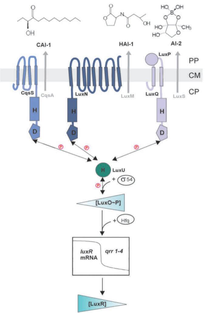
Figure 1. Shows the HAI-1, CAI-1 and AI-2 autoinducers received by kinases/phosphatases LuxN, CqsS and LuxP/Q respectively. The signal transduction pathway regulating the expression of LuxR is also shown via the LuxR transcript. LuxR functions in the regulation of quorum sensing controlled behaviors [4].

Quorum quenching can have a wide range of effects in medicine. It can be responsible for inhibiting biofilm formation and decreasing the pathogenicity of bacteria. Because quorum sensing controls biofilm formation and virulence factor secretion, it has the potential to decrease pathogenicity. For example, the quorum sensing regulated type three secretion system found in many gram-negative bacteria infects eukaryotic cells via the secretion of specific proteins. The quorum quencher naringenin has been shown to decrease the virulence of the type three secretion system [9]. Furthermore, the same quorum sensing pathways control the secretion of exopolysaccharides needed for maintaining biofilm structure [10].

Many quorum sensing pathogens like Vibrio cholerae, Providencia stuartii, Heliobacter pylori and Candida albicans cause harmful infections in humans [2][11][12]. Quorum sensing pathways in these species are analogous to pathways in V. harveyi. Quenching these pathways can be impactful because it offers an alternative approach to target bacterial infections via quorum sensing [2][11]. Quorum quenching works by competitively inhibiting the receptor sites of the autoinducers, degrading autoinducers, or stopping production of autoinducers completely [3][12]. The most effective quorum quenchers are those that inhibit biofilm formation and virulence factor secretion without slowing the growth of bacteria, because inhibiting bacterial growth can lead to more selective pressure and resistance [8].

Many quorum quenching agents have been found in marine organisms and herbal plants [2][11][12]. Some specific plant compounds found to inhibit biofilms are cinnamaldehyde (derived from cinnamon bark extract), neohesperidin and naringenin (both derived from citrus extracts) [9][10]. Cinnamaldehyde works by decreasing the DNA binding ability of the LuxR transcript. Neohesperidin inhibits the efficacy of the HAI-1 autoinducer in V. harveyi. Naringenin inhibits quorum sensing via the AI-2 and HAI-1 autoinducer pathways. Because all three quorum quenchers have different mechanisms of actions in quorum quenching, combinations of these molecules were tested on V. harveyi for possible synergistic effects in the reduction of biofilm formation.

2. Materials and Methods

2.1 – Compounds

Cinnamaldehyde, naringenin and neohesperidin were purchased from Sigma-Aldrich. All compounds were dissolved in dimethyl sulfoxide (DMSO) at a concentration of 10 mg/mL and stored at -20°C.

2.2 – Media and Bacterial Growth

Vibrio harveyi strain BB120 (wild-type) was purchased from ATCC. The Luria Marine (LM) medium was used to grow V. harveyi. Overnignt cultures were incubated at 30°C without shaking.

2.3 – Individual Compound Biofilm Formation Assay

This experiment determined the effect of each of the quorum quenchers individually. Overnight culture of V. harveyi BB120 was diluted in a 1:100 ratio in LM media. One mL of the diluted culture was placed into each well in a 24-well plate. Wells received concentrations of compounds previously found to successfully inhibit quorum sensing in V. harveyi [9][10]. Each well received 6.25 µg/ mL of naringenin, 12.5 µg/mL of neohesperidin, 13.22 µg/ mL of cinnamaldehyde, or 1.32 µL of DMSO as a control. The plates were incubated at 26°C with no shaking for 24

hours to stress bacteria into forming biofilms [9]. The biofilm mass was quantified by Crystal Violet staining. The plates were first washed with deionized water three times. They were then stained with 2 mL of 0.1% Crystal Violet solution for 20 minutes. The dye not associated with the biofilm was washed out with deionized water. All the dye associated with the biofilm was dissolved in 1 mL of 33% acetic acid. The absorbances of these acetic acid and dye samples were taken at 570 nm by a spectrophotometer. The optical density (OD) was used as a means to quantify the biofilm. This experiment was carried out 6 times with 6 replicated wells per plate.

2.4 – Multiple Compounds Biofilm Formation Assay

This experiment determined the effect of combinations of quorum quenching compounds. This was the same assay as Individual Compound Biofilm Formation Assay except each well received 1.32 µL of DMSO as a control, 6.25 µg/mL of naringenin,12.5 µg/mL of neohesperidin, 13.22 µg/mL of cinnamaldehyde, or a combination of the compounds. Combinations tested include cinnamaldehyde/ naringenin and neohesperidin/naringenin. Half concentrations of naringenin (3.125 µg/mL) and cinnamaldehyde (6.61 µg/mL) were tested in later combinations to determine whether a synergistic effect was present. Plates were stained with Crystal Violet and the OD associated with biofilm was measured. Each combination experiment was replicated 3 times with 4 replicated wells per plate.

2.5 – Cellular Growth Assay

This experiment determined whether combinations of compounds altered the growth rates of the bacteria. Overnight culture of V. harveyi BB120 was diluted in a 1:100 ratio in Luria Marine (LM) media. Each tube received either 3.97 µL of DMSO as a control, 6.25 µg/mL of naringenin and 12.5 µg/mL of neohesperidin, 6.25 µg/mL of naringenin and 13.22 µg/mL of cinnamaldehyde, or 6.25 µg/mL of naringenin, 12.5 µg/mL of neohesperidin and 13.22 µg/ mL of cinnamaldehyde. The cultures were grown for 24 hours at 30°C with shaking. Optical densities of the broth were taken roughly every 2 hours for the first 8 hours. Additionally, samples were taken of the broth at 6 hours and 24 hours. The samples were serially diluted and plated on LM agar plates and colony forming units were counted after 24 hours of growth. This experiment was replicated twice.

3. Data Analysis

To analyze the results of my experiments, the statistical software JMP 10 was used to run ANOVA tests and first determine the presence of a treatment effect. If the ANOVA test showed an effect, a Tukey’s Honest Significance Difference (HSD) test was conducted to discern the significant differences among means. Some data were additionally graphed as percent biofilm inhibition, further emphasizing the presence of a synergistic effect. Biofilm inhibition percentages were calculated as (control OD - treatment OD)/(control OD)*100.

4. Results

4.1 – Individual Compound Biofilm Formation Assay

To measure the effectiveness of individual plant-derived compounds on quorum sensing inhibition, the individual compound biofilm formation assay was conducted on V. harveyi biofilms. As determined by the Tukey’s honest significance test, naringenin at a concentration of 6.25 µg/mL significantly decreased biofilm mass. Cinnamaldehyde and neohesperidin showed no detectable biofilm inhibition (Fig 2).

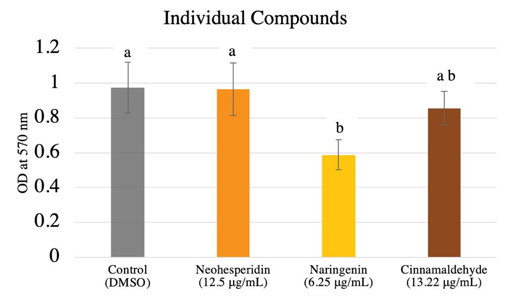
Figure 2. Individual Compound Biofilm Formation Assay. Shows the results of the individual plant-derived compounds on biofilm formation in V. harveyi to see which compounds were most effective. Error bars show mean +/- 1 SEM. An ANOVA test was conducted and showed p < 0.0037* (Table 1). A Tukey’s Significance test was then conducted. Different letters correspond to significant differences as discerned by Tukey’s HSD test.

Table 1. ANOVA table from the Individual Compound Biofilm Formation Assay (Fig. 2). Source DF Sum of Mean F Ratio Prob > F Squares Square

Compound

3 0.34467 0.11489 6.2299 0.0037*

Error 20 0.36883 0.018442

Corr. Total

23 0.7135

4.2 – Multiple Compounds Biofilm Formation Assay

Because naringenin was consistently effective, combinations with naringenin were tested. The cinnamaldehyde and naringenin combination (Fig. 3a) showed a significant

difference between the control and the individual compounds, but no significant difference between the combination and the individual compounds, which is indicative of naringenin overpowering the combination.

a)

b)

Figure 3. Combinations with naringenin. a) Shows V. harveyi biofilm formation when treated with the combination of cinnamaldehyde and naringenin. Naringenin concentrations were 6.25 µg/mL and cinnamaldehyde concentrations were 13.22 µg/mL. The ANOVA test showed p < 0.0002* (Table 2), indicating that there is indeed some difference between the compounds. The Tukey’s HSD test was then conducted to find specific differences. b) Shows V. harveyi biofilm formation when treated with the combination of naringenin and neohesperidin. The ANOVA test showed p < 0.0001* (Table 3), indicating that there is indeed some difference between the compounds. Tukey’s HSD test was then conducted to find specific differences. Different letters on the graphs above indicate differences in significance according to Tukey’s HSD test.

The neohesperidin and naringenin combination (Fig. 3b) showed naringenin significantly different from the control and neohesperidin indistinguishable from the control. Furthermore, the combination of naringenin and neohesperidin was indistinguishable from naringenin, supporting the theory that neohesperidin showed no detectable effect. In these combinations the raw OD values of

Table 2. ANOVA test conducted on the combination of naringenin and cinnamaldehyde (Fig. 3a). Source DF Sum of Mean F Prob > F Squares Square Ratio

Compound

3 0.34688 0.11562812.07780.0002*

Error 17 0.16275 0.009574

Corr. Total

20 0.50963

Table 3. ANOVA test conducted on the combination of neohesperidin and naringenin (Fig. 3b). Source DF Sum of Mean F Prob > F Squares Square Ratio

Compound

3 0.41184 0.11562817.9586 0.0001*

Error 20 0.15289 0.009574

Corr. Total

23 0.56473

the combinations were low, so in subsequent experiments biofilm formation was increased through less volume of LM media in all the wells to better detect an inhibitory effect of the combinations. Since naringenin seemed to overpower combinations, half the concentration of naringenin (3.125 µg/mL) was tested with cinnamaldehyde (Fig. 4). The combination with full concentrations of naringenin and cinnamaldehyde showed a significant difference in biofilm formation compared to the other individual compounds, suggesting an interaction between the compounds. Because this combination had a greater percent biofilm inhibition than the individual compounds’ percents of inhibition combined (Fig. 5), it was concluded that a synergistic effect was present. However, the combination with half the concentration of naringenin and full concentration of cinnamaldehyde was indistinguishable from the full concentration of naringenin alone, showing the necessity of naringenin for the synergy (Fig. 5). A similar experiment was conducted to determine the effects of cinnamaldehyde concentration on this synergy by testing combinations of naringenin with half the concentration of cinnamaldehyde (6.61 µg/mL). A synergistic effect was present in the combinations of naringenin with both full and half concentrations of cinnamaldehyde, indicating that the concentration of cinnamaldehyde is not as integral as that of naringenin for the synergy (Fig. 6 and 7).

Figure 4. Combinations with Varied Concentrations of Naringenin. Effects on biofilm formation of the combination of naringenin at full (6.25 µg/mL) and half (3.125 µg/mL) concentrations with cinnamaldehyde (13.22 µg/mL). Error bars show 1 SEM. ANOVA test p < 0.0001* (Table 4). Letters correspond to differences discerned by Tukey’s HSD Test.

Table 4. ANOVA test conducted on full concentrations of cinnamaldehyde with varied concentrations of naringenin (Fig. 4). Source DF Sum of Mean F Prob > F Squares Square Ratio

Compound

5 0.94506 0.18901129.7551<0.0001*

Error 18 0.11434 0.006352

Corr. Total

23 1.0594

Figure 5. Percent Biofilm Inhibition of Varied Naringenin Concentrations. Biofilm inhibition percentages calculated as (control OD - treatment OD)/(control OD)*100. Error bars show 1 Standard Error of the Mean (SEM). Figure 6. Combinations with Varied Concentrations of Cinnamaldehyde. Effects on biofilm formation of the combination of cinnamaldehyde at full (13.22 µg/ mL) and half (6.61 µg/mL) concentrations with naringenin (6.25 µg/mL). Error bars show 1 SEM. ANOVA test p < 0.0001* (Table 5). Letters correspond to differences discerned by Tukey’s HSD Test.

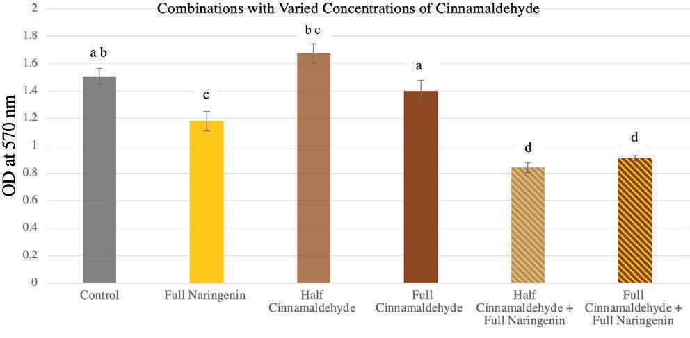
Table 5. ANOVA test conducted on full concentrations of naringenin tested with various concentrations of cinnamaldehyde (Fig. 6). Source DF Sum of Mean F Prob > F Squares Square Ratio

Compound

5 2.21176 0.4423 31.761 <0.0001*

Error 18 0.25065 0.0139

Corr. Total

23 2.4624

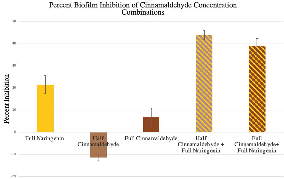
Figure 7. Percent Biofilm Inhibition of Varied Cinnamaldehyde Concentrations. Shows the biofilm inhibition percentages calculated as (control OD - treatment OD)/(control OD)*100. Error bars show 1 SEM.

4.3 – Multiple Compounds Cellular Growth Assay

The experiment was conducted to show the growth rate of the V. harveyi bacteria when treated with combinations used in biofilm formation assays. Because the growth rates

of bacteria remained unchanged when treated with combinations of compounds, it is understood that the treatments are inhibiting only quorum sensing, not altering the mortality of V. harveyi.

Figure 8. Cellular Growth Assay. Shows the growth curve of V. harveyi treated with DMSO (control), cinnamaldehyde (13.22 µg/mL)/naringenin (6.25 µg/mL), neohesperidin (12.5 µg/mL)/naringenin (6.25 µg/mL)/ cinnamaldehyde (13.22 µg/mL), neohesperidin (12.5 µg/mL)/naringenin (6.25 µg/mL). Error bars show mean +/- 1 SEM.

5. Discussion

The results of our study showed naringenin alone was able to inhibit biofilm formation, whereas neohesperidin and cinnamaldehyde alone at the concentrations tested showed no consistent detectable effect on biofilm inhibition (Fig. 2). This study confirmed previous studies showing that naringenin strongly suppressed AI-2 and HAI-1 mediated quorum sensing in V. harveyi. Because cinnamaldehyde was thought to inhibit the master regulatory protein LuxR, it was hypothesized to be the most effective. However, the variable effects of cinnamaldehyde as well as the consistently undetectable effects of neohesperidin, responsible for the inhibition of HAI-1 mediated quorum sensing, were unexpected. Surprisingly, there was a synergistic effect present when both cinnamaldehyde and naringenin were used to inhibit biofilm formation. It is important to note the combinations of cinnamaldehyde/ naringenin and neohesperidin/naringenin showed low raw OD values. Only 1 mL of LM media was administered to each well in later experiments to increase baseline biofilm formation, so inhibition could more easily be detected. In the earlier experiments, naringenin seemed to overpower combinations as the combination was not significantly different from naringenin alone. Therefore, half concentrations of naringenin were tested with decreased media per well. Synergy was detected with the full concentration of cinnamaldehyde and naringenin.

One explanation for this synergy is that once naringenin blocks AI-2 and HAI-1 mediated quorum sensing, cinnamaldehyde is left to inhibit only the effects of CAI-1 mediated quorum sensing (Fig. 1). Cinnamaldehyde may be more effective at decreasing the DNA-binding affinity of relatively small amounts of LuxR, which would explain the apparent synergy and why the synergy depended heavily on the concentration of naringenin present. It is also possible that there are more components to this pathway. If naringenin inhibits other unknown components of this pathway that cinnamaldehyde cannot, cinnamaldehyde alone might be ineffective because of the activation of multiple components of the pathway. The inconsistent results of cinnamaldehyde could be explained by the presence of these additional, confounding components. In combinations, however, naringenin could block the unknown components and cinnamaldehyde would be able to work effectively. In addition, it is confirmed that these compounds inhibit only quorum sensing and not cell growth rates because results of the cellular growth assay show a similar curve with and without the treatments (Fig. 8).

Future directions include altering the concentrations of quenchers to see if greater inhibition and optimization are possible, elucidating the exact mechanisms of these quorum quenchers, and observing the effects of combinations of different quorum quenchers on biofilm formation. It would be interesting to see which autoinducers contribute the greatest effect on biofilm formation by testing combinations of naringenin or cinnamaldehyde with a quorum quencher that acts on CAI-1 mediated quorum sensing. Another approach would be to test knockout strains of V. harveyi that only respond to AI-2 and HAI-1 mediated quorum sensing to see if decreased biofilm formation occurs. As further research ensues, the mechanisms of the quorum quenchers will be better known and can be optimized in combinations to produce more synergistic effects on decreasing biofilm formation.

More broadly than decreasing biofilm formation, quorum sensing inhibition has the potential to act as an alternative to antibiotics. Because quorum quenching effectively reduces biofilm formation and does not kill bacteria, it can be a less selective alternative therapy to antibiotics [12]. Since quorum sensing controls not only biofilm formation but also the secretion of other virulence factors [2], the inhibition of quorum sensing can decrease virulence factor production. The production of these factors can also be measured to detect synergistic effects among quorum quenchers. The applications of this project are in inhibiting biofilm formation, which can be used as the foundation for biofilm-resistant hospital materials, alternative antibiotic treatments or as a model for V. cholera. These applications are important as a model for V. cholera because the V. cholera biofilm plays a critical role in pathogenesis and disease

transmission [13]. A cholera outbreak occurred in Haiti in 2010 when UN peacekeepers introduced the disease to the earthquake devastated country, taking upwards of 10,000 lives. In 2018, there were cholera outbreaks in Yemen and Somalia. Additionally, costs of outbreaks were estimated to be $38.9-$64.2 million in 2005 [14]. Through further studying this synergistic effect of quorum quenchers on decreasing biofilm formation in V. harveyi, the mortality rates and economic costs due to infectious diseases including cholera can decrease in the future.

6. Acknowledgments

This work would not have been possible without the endless guidance and support of my mentor, Amy Sheck. I would like to extend gratitude to Kimberly Monahan, as well. Also, I would like to thank Nick Koberstein for help with statistical analysis. Furthermore, I would like to thank the Research in Biology Classes of 2019 and 2020 for their friendship and advice. Lastly, I am highly indebted to the Glaxo Endowment to the North Carolina School of Science and Mathematics for providing the funding for this project.

7. References

[1] Bassler, B. L. & Losick, R. (2006) Bacterially speaking. Cell, 125, 237-246.

[2] Defoirdt, T. (2017) Quorum-sensing systems as targets for antivirulence therapy. Trends in Microbiology, 26, 313328.

[3] Vadakkan, K., Choudhury, A. A., Gunasekaran, R., Hemapriya, J. & Vijayanand, S. (2018) Quorum sensing intervened bacterial signaling: pursuit of its cognizance and repression. Journal of Genetic Engineering and Biotechnology, 16, 239-252.

[4] Anetzberger, C., Pirch, T. & Jung, K. (2009) Heterogeneity in quorum sensing-regulated bioluminescence of Vibrio harveyi. Molecular Microbiology, 73(2), 267-277.

[5] Tu, K. C. & Bassler, B. L. (2007) Multiple small RNAs act additively to integrate sensory information and control quorum sensing in Vibrio harveyi. Genes Dev, 21, 221-223.

[6] Brackman, G., Deifoirdt, T., Miyamoto, C., Bossier, P., Calenbergh, S. V., Nelis, H., & Coenye, T. (2008) Cinnamaldehyde and cinnamaldehyde derivatives reduce virulence in Vibrio spp. by decreasing the DNA-binding activity of the quorum sensing response regulator LuxR. BMC Microbiology, 8, 149-163. [7] Lilley, B. N. & Bassler, B. L. (2000) Regulation of quorum sensing in Vibrio harveyi by LuxO and Sigma-54. Molecular Microbiology, 36, 940-954.

[8] Kalia, V. C., Patel, S. K. S., Kang, Y. C., & Lee, J. (2019) Quorum sensing inhibitors as antipathogens: biotechnological applications. Biotechnology Advances, 37, 68-90.

[9] Vikram, A., Jayaprakasha, G. K., Jesudhasan, P. R., Pillai, S. D. & Patil, B. S. (2010) Suppression of bacterial cell-cell signaling, biofilm formation and type III secretion system by citrus flavonoids. Journal of Applied Microbiology, 109, 515-527.

[10] Packiavathy, I. A. S. V., Sasikumar, P., Pandian, S. K., & Ravi, A. V. (2013) Prevention of quorum-sensing-mediated biofilm development and virulence factors production in Vibrio spp. by curcumin. Applied Microbiology and Biotechnology, 97, 10177-10187.

[11] Ta, C. A. K. & Arnason, J. T. 2015. Mini review of phytochemicals and plant taxa with activity as microbial biofilm and quorum sensing inhibitors. Molecules, 21, E29.

[12] Kalia, V.C. (2013) Quorum sensing inhibitors: an overview. Biotechnology Advances, 31, 224-245.

[13] Silva, A. J. & Benitez, J. A. (2016) Vibrio cholera Biofilms and Cholera Pathogenesis. PLOS Neglected Tropical Diseases, 10(2), e0004330.

[14] Tembo, T., Simuyandi, M., Chiyenu, K., Sharma, A., Chilyabanyama, O. N., Mbwili-Muleya, C., Mazaba, M. L., & Chilengi, R. (2019) Evaluating the costs of cholera illness and cost-effectiveness of a single dose oral vaccination campaign in Lusaka, Zambia. PLOS One, 14(5), e0215972.

EMOTIONAL PROCESSING AND WORKING MEMORY IN SCHIZOPHRENIA WITH NEUTRAL AND NEGATIVE STIMULI: AN fMRI STUDY

Cindy Zhu

Abstract

Schizophrenia (SZ) is a psychiatric disorder that results in abnormalities with emotional processing and working memory. Working memory (WM) and Emotional Processing (EP) are supported by specific neural regions in the brain; however, we do not know how these regions interact to influence task performance. To explore the effects of emotional valence on working memory, an emotional n-back task was used with a focus on Neutral and Negative emotional valence and on working memory and emotional processing regions in the brain. In the neutral condition, we observed recent-onset schizophrenia (RO) participants having a lower activation than genetic high-risk (HR) participants in working memory regions (ACC, Left ACC, Right ACC), and in ventral regions (Left NAcc). RO showed lower activation than control (CON) participants in the Left DLPFC. These results align with behavioral results - RO did not show a significant difference in D′ values between Neutral and Negative conditions while controls did, which may reflect the belief that RO patients have a greater ability to focus on the working memory task due to tunneling and focus less on the emotional valence as compared to the control patients. When exploring the correlation between brain activity and task performance, we found CON and RO exhibiting a positive correlation, while HR showed a negative correlation. In conclusion, during a cognitively demanding task, RO participants exhibit fewer differences in working memory and emotional regulation between conditions, which supports prevailing theories of emotional blunting and tunneling. In addition, surprising differences between HR and RO groups showed HR with overactivation, as opposed to prevailing theories that HR will show levels of activation intermediate between CON and RO.

1. Introduction

Schizophrenia is characterized by significant impairments in working memory and emotional regulation. Impairments in working memory (WM), the temporary storage and manipulation of information held for a limited period of time, are considered a core neurocognitive deficit in patients with schizophrenia (SZ) and can significantly impact quality of life. Deficits in emotional regulation, or the conscious effort in modulating emotional response to goal-unrelated or irrelevant emotional stimuli, interfere with social life and daily functioning, and may also be associated with the development of psychotic symptoms [1]. These deficits in WM are present prior to the onset of illness, such as in genetically high-risk individuals, or in patients who are medication-free in their first episode of illness [2]. Thus, gaining a better understanding of the interplay of emotional regulation and working memory in patients with schizophrenia may help improve patient diagnosis and quality of life.

Emotional blunting, or blunted affect, is one of the core negative symptoms of schizophrenia and results in difficulty in expressing emotions in reaction to emotional stimuli due to problems with emotional processing. There are mixed findings of activation during emotionally evocative stimuli between people with and without schizophrenia in areas associated with emotion, with some studies reporting no differences in activation, while others report diminished activation [3]. Emotional processing abnormalities in schizophrenia have been shown to reduce activation in brain regions associated with emotional processing in response to emotionally evocative stimuli [4]. It remains unclear how these alterations in emotional valence processing may impact WM functions for individuals with schizophrenia.

Working memory is an important component of higher cognition, such as goal-directed behavior. Deficits in schizophrenia may relate to a number of other core symptoms in schizophrenia [5]. Working memory impairment is often associated with differing DLPFC activation, which is implicated in executive functions, goal-directed planning, and inhibition, and is a part of working memory circuitry [6]. The effects of these deficits can be studied using n-back tasks, which test working memory by utilizing continuous updating and order memory [2].

Emotional regulation processes and working memory can be studied in conjunction using emotional working memory paradigms through functional magnetic resonance imaging (fMRI). Task-based fMRI allows for both behavioral and aggregate neural activation measurements and can help identify how emotion and WM interact. An emotional one-back task was used with neutral and negative conditions. Participants were instructed to indicate when a new stimulus (image with emotional valence) was the same as the stimulus presented one before, which required short-term memory engagement. By using an

emotional one-back task, the influence of the emotional valence (i.e. whether a stimulus is neutral or negative) on WM can be calculated.

The influence of emotion on cognition is an essential topic to research, but research on this topic has received less attention than others in schizophrenia literature. In controls, it has been shown that emotional stimuli can garner more attention than neutral stimuli. This extra attention may facilitate the processing of emotional stimuli. In patients with schizophrenia, there may be reduced activation and worsened performance due to the addition of emotional valence to the WM task. DLPFC has an important role in the integration of emotional and cognitive information [7]. Studies of negative valence and cognition tend to produce more robust results due to the arousing nature of the images used. Other studies [4] also explore the interaction between EP and WM, but only with control and schizophrenia patient groups. By including HR participants, which have been found to show similar working memory deficits as those with schizophrenia [2], in our study of the interaction of WM and EP, we address a new set of questions in how high-risk participants perform compared to controls and RO and if they exhibit deficits similar to RO participants.

The overarching goal of this study is to identify how WM and emotional processes interact, particularly in the context of schizophrenia. In order to achieve this aim, we administered an emotional n-back task to 76 participants (35 control, 20 HR, 21 RO) to determine group differences in regional activation and WM performance associated with psychotic illness. We hypothesized that RO participants would perform consistently across neutral and negative conditions (because emotional blunting may result in less expressed performance differences between valences), while control participants would have more impaired performance in the negative condition compared to the neutral condition. Moreover, we hypothesized that changes in performance between conditions will differ between subject groups. When looking at brain activation, we hypothesized that the control participants would exhibit a greater change in ventral regions when comparing between the neutral and negative conditions and that control participants would have a greater change in activation in WM regions between neutral to negative. We also hypothesized that genetic high-risk participants would exhibit brain activation and task performance intermediate between CON and RO. Finally, we investigated links between activation and behavior to see if changes in activation correlated with changes in task performance.

2. Methods

2.1 – Participants

Twenty-one patients with recent-onset schizophrenia and twenty genetic high-risk patients were recruited from the UNC Healthcare System. Thirty-five healthy control subjects were also included. All participants provided written consent to the study approved by the University of North Carolina- Chapel Hill IRB. All participants were between the ages of 16-45, of any ethnicities or gender, had no presence of metallic implants or devices interfering with MRI, and were not pregnant. Inclusion criteria for recent-onset schizophrenia (RO) patients were: (1) Meet DSM-IV criteria for SZ or schizophreniform disorder, (2) No history of major central nervous system disorder or intellectual disability (IQ<65), (3) Must have illness for <5 years, (4) No current diagnosis of substance dependence, and no substance abuse for 6 weeks. RO patients were also instructed to refrain from taking benzodiazepine medications on the morning of testing but instead to bring their medication with them to take after scanning. Inclusion criteria for genetic high risk (HR) patients were: (1) Must have first degree relative with psychotic disorder, (2) Must not meet DSM-IV criteria for past or current Axis I psychotic disorder on bipolar affective disorder, (3) No history of major central nervous system disorder or intellectual disability (IQ<65), (4) No current treatment with antipsychotic medication. Healthy controls (CON) were excluded if they had history of a DSM-IV axis I psychiatric disorder, family history of psychosis, history of current substance abuse/dependence, history or current medical illness that could affect brain morphology, or clinically significant neurological or medical problems that could influence the diagnosis or the assessment of the biological variables in the study. All participants gave written informed consent consistent with the IRB of UNC if over 18 or assent and parent/guardian provided consent for minors prior to their participation in the study.

2.2 – Emotional One-back Task and Procedure

Each participant completed an emotional one-back task with an auditory component during a functional magnetic imaging (fMRI) session with 8 runs. The emotional oneback task consists of a visual tracking task, using images with either Positive, Neutral, or Negative valence, as defined by the International Affective Picture System (IAPS) [8]. Further analysis was performed with only Neutral and Negative Valences. Patients with schizophrenia report feeling negative emotion strongly but are less outwardly expressive of this negative emotion [9]. By focusing on the Negative valence, we want to observe if RO exhibit similar activation to CON during negative emotional situations, as the contexts in which RO patients experience negative emotion is different than those without SZ. All images in the run were of the same valence, and subjects were asked to press a button when they saw the same image two times in a row (Fig. 1). A control condition with no n-back task was also included. The auditory component, which occurred simultaneously with the visual component, involved subjects hearing irrelevant standard and pitch devi-

ant tones at random intervals, but for the study’s purposes, it was excluded from further analysis.

The task was divided into 8 runs, with 2 runs of each valence, and 2 control runs with no n-back task. Each run lasted 200.58s, with 14 target images, 56 non-target images. Each image was presented for 500ms and the inter-stimulus interval was either 1500ms or 3000ms.

Figure 1. Emotional One-Back Task. Participants were asked to press a button when the picture shown matches the picture shown one before.

2.3 – Behavioral Analysis

To analyze the performance of participants during the task, D′, or sensitivity index, was used as a metric, because it considers accuracy and sensitivity. Paired t-tests were performed to investigate within-group differences in D′ between Neutral and Negative task conditions. To investigate differences between groups (CON, HR, and RO) and condition (Neu and Neg) and the interaction effects of both factors on D′, a 2-way ANOVA was used. Finally, a one-way ANOVA was used to investigate group differences for neutral and negative conditions, only considering one condition at a time. A Tukey comparison of means was performed for One-way and Two-way ANOVA’s that had significant results to further interpret the results.

2.4 - Neuroimaging Analysis 2.4.1 - Imaging Data Acquisition

A General Electric 3.0 T MRI scanner with a functional gradient-echo echo-planar imaging sequence allowing for full-brain coverage (TR: 2000 ms; TE: 27 ms; FOV: 24 cm; image matrix: 64×64; flip angle: 60; voxel size: 3.75×3.75×3.8mm3; 34 axial slices) was used. Each functional run had 120 time-points. Structural MRIs were acquired before fMRIs to obtain 3D coplanar anatomical T1 images using a spoiled gradient-recalled acquisition pulse sequence (TR: 5.16 ms; TE: 2.04 ms; FOV: 24 cm; image matrix: 256×256; flip angle: 20; voxel size: 0.94×0.94×1.9 mm3; 68 axial slices).

2.4.2 - Preprocessing

Functional data analyses were carried out using the University of Oxford’s Center for Functional Magnetic Resonance Imaging of the Brain (FMRIB) Software Library (FSL) release 6.0 [11]. Image preprocessing consisted of using the Brain Extraction Tool (BET) to remove nonbrain structures, motion correction, time-slice correction and spatial filtering using a Gaussian kernel of full width half maximum 5 mm, high-pass temporal filtering. The functional images were co-registered to the structural images in their native space. These images were then normalized to the Montreal Neurological Institute standard brain. The default adult template in FMRIB’s Linear Image Registration Tool (FLIRT) was used for registration [10]. FMRIB’s Improved Linear Model (FILM) was used for pre-whitening in order to estimate and account for each voxel’s time series auto-correlation.

2.4.3 - Whole Brain Analysis

Whole Brain Analysis was performed to ensure that the tasks activated regions known to be involved in WM and EP. These whole-brain maps were thresholded for significance to obtain a significant rate of p=0.05 (corrected for false discovery rate due to multiple comparisons) with Randomise, which tests for correlation inferences using permutation methods, implemented in FSL [11]. The Dorsal Attention and Ventral Attention networks [12] were used to check that existing patterns of activation in control participants were consistent with working memory and emotional processing regions. The control mean group activation was then overlaid on top of the two attention networks to see where activation overlapped.

2.4.4 - Region of Interest Selection

Regions of Interest (ROI) involved in working memory circuitry and/or emotional processing were selected (Fig. 2). Dorsal, or working memory regions, include the whole anterior cingulate cortex (ACC), left and right anterior cingulate cortex (Left ACC, Right ACC), left and right dorsal lateral prefrontal cortex (Left DLPFC, Right DLPFC), and the interparietal sulcus (IPS). Ventral regions, or regions involved in emotional processing, include left and right amygdala (Left AMY, Right AMY), left and right nucleus accumbens (Left NAcc, Right NAcc), and left and right Orbitofrontal cortex (Left OFC, Right OFC).

2.4.5 - fMRI Statistics

Using FSL version 6 [11], the FEAT first-level analysis was performed on each run per subject, where a general linear model is used to model the expected hemodynamic response function, which models the evoked hemodynamic response to a neural event. In the second-level analysis, three contrast of interest (Neutral, Negative, Neutral > Negative) were generated for each subject across multiple runs to investigate the interaction between emotional valence and type of model design (NeuVisTarg > NegVisTarg or NeuVis > NegVis), and each emotional valence and type of model design (NeuVisTarg and NegVis). In the final analysis, only event designs Neutral, Negative, and Neutral>Negative contrasts were considered.

Table 1: Demographic information for the participants. CON denotes Healthy controls, HR denotes High Risk Participants and RO denotes Recent Onset Participants. CON (n=35) HR (n = 20) RO (n = 21) Mean SD/% Mean SD/% Mean SD/% p(CON-HR) p(CON-RO) p(HR-RO)

Age 27.01 6.07 30.62 7.89 25.29 4.92 0.068 0.284 0.015 Male 19 54.29% 5 25% 17 80.95% 0.037 0.0457 0.0004 Female 16 45.71% 15 75% 4 19.05% 0.037 0.0457 0.0004

These contrasts were then submitted to the third level analysis to examine differences between groups in task-related brain activity. Region of Interest analysis was then conducted using FEATQUERY, and beta values, which represent the direction and magnitude of regional brain activation, were extracted from working memory (WM) and emotional processing (EP) of the brain.

We conducted paired t-tests to investigate the differences between neutral and negative conditions within the same subject group. To investigate differences between groups (CON, HR, and RO) and condition (Neu and Neg) and the interaction effects of both factors, a 2-way ANOVA was used. Finally, a one-way ANOVA was used to investigate group differences for neutral and negative conditions for different regions. Post Hoc analysis was performed with a Tukey comparison of means for one way and Two-way ANOVA’s that had significant results, in order to isolate specific effects (or differences).

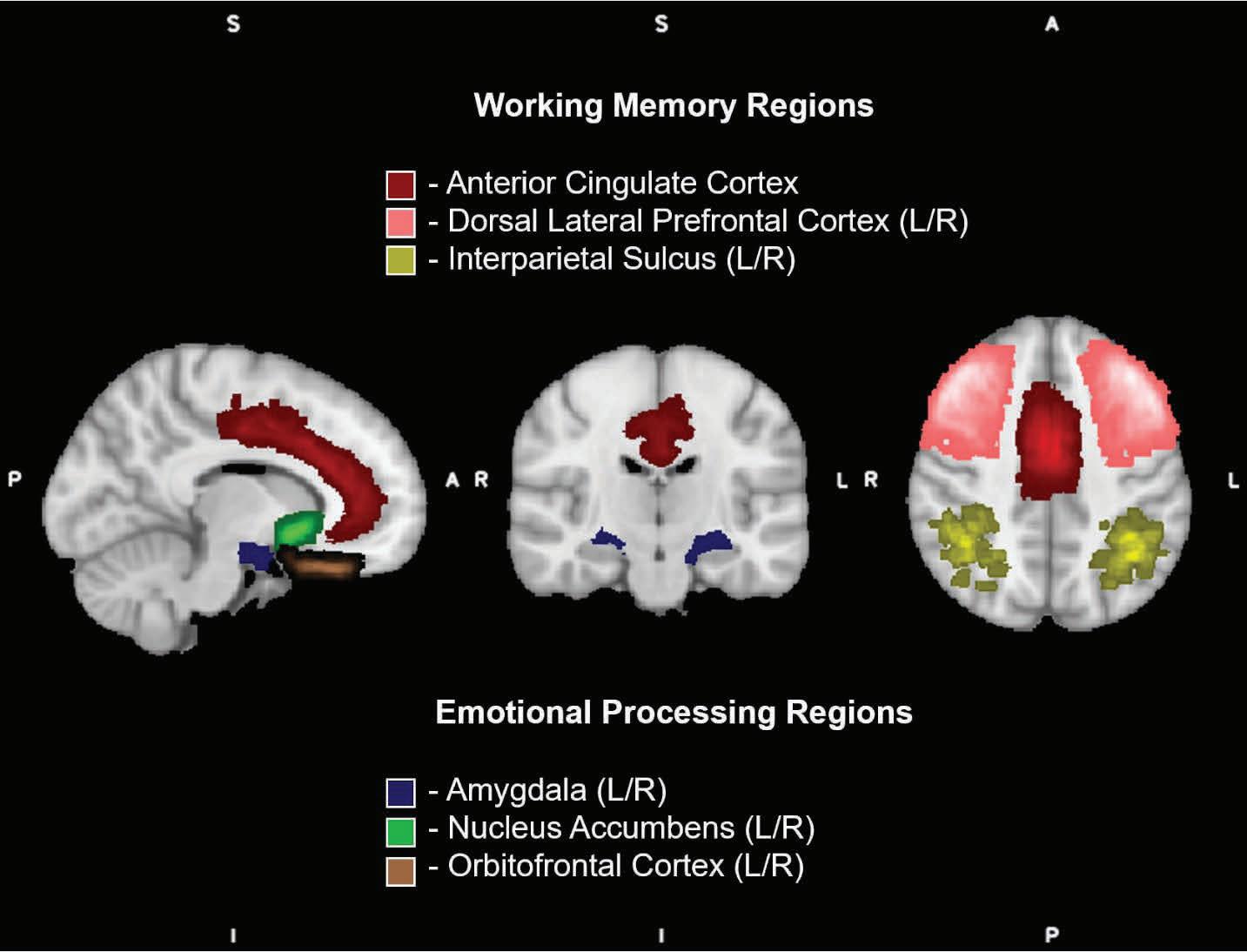
Figure 2. Regions of Interest used in Analysis.

2.5 - Brain Activity and WM Performance

In order to explore links between brain activity and WM performance, linear regression was performed with extracted beta values from selected ROI and neutral and negative conditions as the independent variable and D′ values as the dependent variable. Subjects without behavioral data were excluded. These regressions were performed on patient groups (CON, RO and HR participants) and the correlation was identified.

3. Results

3.1 - Basic Information

The demographic information of these three groups (Healthy Controls, High-Risk participants, and Recent Onset Participants) are listed in Table 1. There was no significant difference between CON and RO regarding age. However, there is a significant age difference between CON-HR and HR-RO, which may be due to the greater ages of the HR participants. High-Risk participants may be of greater age because the tendency for schizophrenia to manifest in patients in their late teens or early twenties does not restrict the pool of HR participants. As a result, there is a wider age range for HR participants to be chosen from (unrestricted by diagnosis), while recent-onset schizophrenia typically occurs before the age of 35, which may explain the difference in mean age. There is a significant difference between all groups (CON-HR, CON-RO, RO-HR) regarding sex (male and female). This is due to the high percentage of Male RO and a high percentage of Female HR.

3.2 - Behavioral Performance on the Emotional One-back Task 3.2.1- Within-Group Analysis

Control participants performed significantly worse during the neutral valence than the negative valence (t = -2.216, p = 0.035) but the recent-onset and high-risk participants exhibited no significant difference in performance between the neutral and negative valences (Fig. 3).

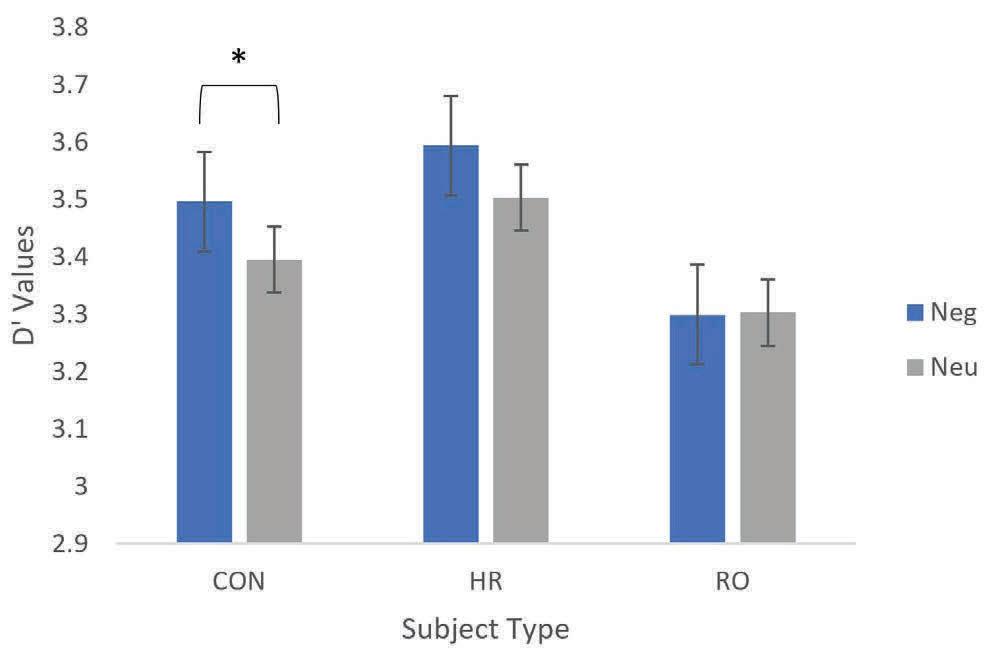
Figure 3. Within Group D′ Values for Neutral and

Negative Condition.

3.2.2 - Between-Group Analysis

A Two-way ANOVA with D′ as the dependent variable revealed no significant main effects, including Subject Group, Valence, and Subject Group by valence interaction. While not significant, the HR group had the best task performance (highest group mean D′), followed by the control group and lastly the RO group.

3.3 - Whole Brain Imaging Analysis

For Neutral and Negative conditions, the activation of the control means overlapped with dorsal and ventral regions. Some specific regions include the anterior cingulate cortex and the intraparietal sulcus. Neutral>Negative exhibited less overlap, but since this condition is calculated from the difference between Neutral and Negative, it is expected that there would be lower activation in those regions. Activation in visual regions is expected given that it is a visual task (i.e. the occipital activation).

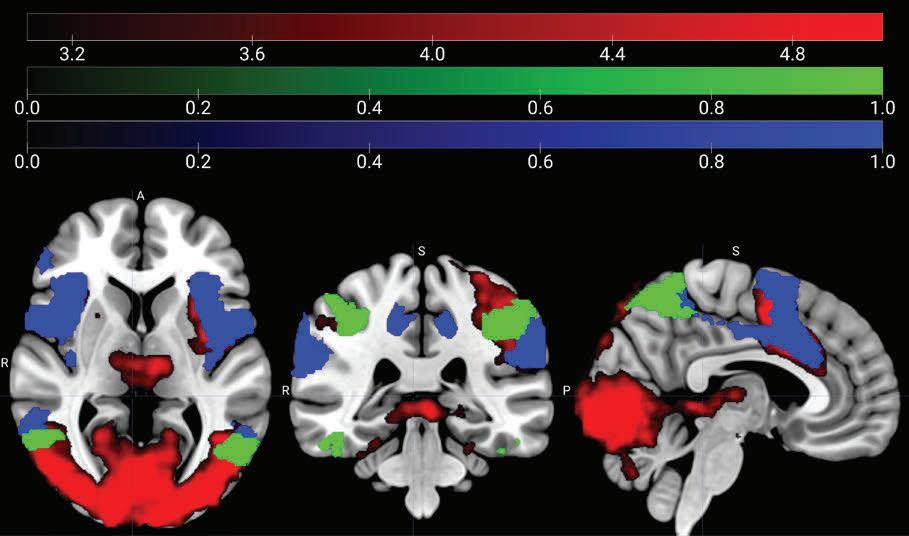
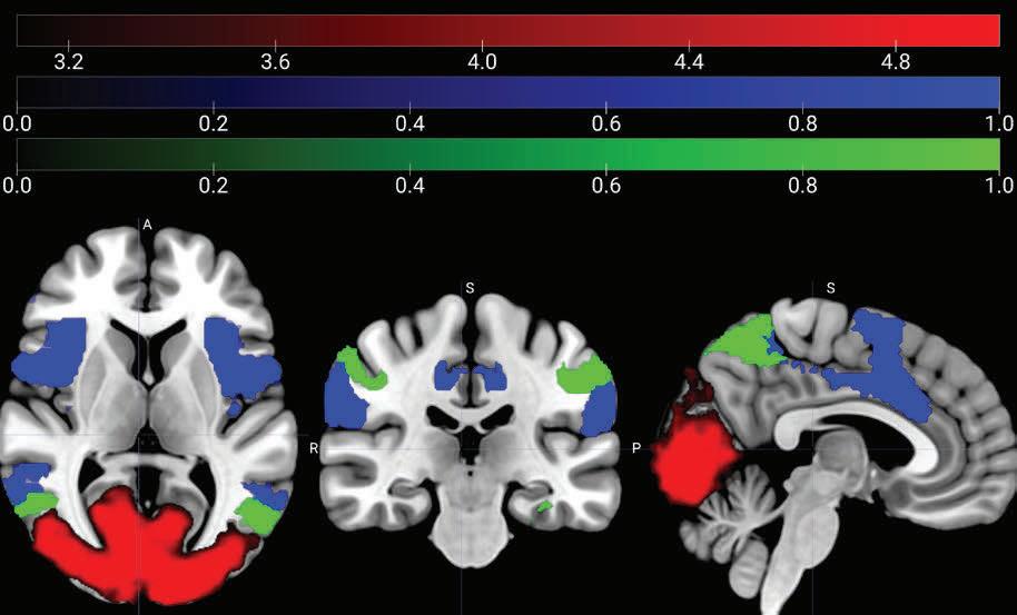
a) Neutral Condition b) Negative Condition c) Neutral > Negative Condition Figure 4. Whole Brain Results showing Mean Control Activation across conditions.

3.4 - Region of Interest Analysis 3.4.1 - Within-Group Analysis

CON, HR and RO subjects did not show significant within-group changes in activation between Neutral and Negative valence in Dorsal or Ventral Regions (Fig. 5). While not significantly different, in control participants, all regions but the left AMY had greater activation in the Neutral condition. In high-risk participants, all dorsal regions but the left and right DLPFC had greater activation in the Neutral condition, and in ventral regions, all but the left AMY and left NAcc had greater activation in the Negative condition. Finally, in recent-onset participants, all dorsal regions but the right ACC and right DLPFC had greater activation in the Negative condition and all ventral regions but the right AMY had greater activation in the Negative condition.

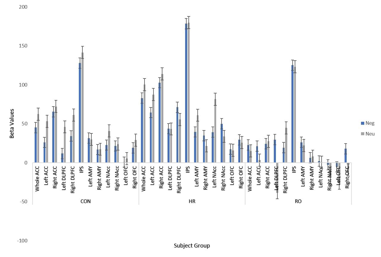
Figure 5. Within-Group Average Beta Values for Neutral and Negative Condition.

3.4.2 - Between-Group Analysis

We observed significant main effects of group in working memory regions, specifically ACC (F=4.158, p=0.018), Left ACC (F=3.434, p=0.0348), and Right ACC (F=4.3281, p=0.015). Upon further investigation, the group difference lies between RO and HR groups in the Neutral condition, with greater activation in the HR group (Table 2). We also observed significant main effects in emotional processing regions, specifically, Left NAcc (F = 4.4413, p= 0.013). Similarly in the Left NAcc, the group difference lies between RO and HR groups in the Neutral condition, with greater activation in the HR group (Table 2). As a follow-up analysis of the Two-way ANOVA, the One-way ANOVA was used to identify which valence the significant differences found with the Two-way ANOVA were associated with. There was a significant difference between groups in the Left DLPFC during the Neutral condition (F=4.0098, p=0.02227). After performing post-hoc analysis, the difference was shown to be between the RO and CON groups, with RO having significantly less activation than CON (Fig. 6). The examination of beta values suggests differences in the Neutral condition may be driven

Table 2. Significant 2-way ANOVA and Post-Hoc Test Results 2-way ANOVA Region F value p-value Group Sig. Diff Tukey Comparison of Means p-value Greater Activation

ACC 4.158 0.018 HR-RO 0.013 HR

Left ACC 3.438 0.035 HR-RO 0.027 HR

Right ACC 4.328 0.015 HR-RO 0.011 Left NAcc 4.4413 0.013 HR-RO 0.009 HR HR

by greater deactivation or less activation for RO subjects in dorsal and ventral regions. While not significant, HR and Control activation is greater than RO for all regions in the Neutral condition. HR shows the greatest activation across all regions except the Left DLPFC (control greater), while controls show greater activation than RO in all regions.

In the Negative condition, there are no significant differences between groups. HR shows greater activation in all regions, while controls show greater activation than RO in all regions but the Left DLPFC. Finally, to assess the change in activation from the Neutral condition to the Control condition, Neutral > Negative activation was evaluated. While there were no significant differences between groups, in dorsal regions except for the right DLPFC and the IPS, RO exhibited greater deactivation. This deactivation can be attributed to RO having greater activation in Negative conditions than Neutral conditions for those regions.

3.5 - Brain Activity and Task Performance

We explored the impact of brain activity in working memory and emotional processing regions on participants’ performance by the subject group during Neutral and Negative conditions. For control participants, there was a significant link between activation and task performance in the Right NAcc in the Neutral condition. This linear relationship (t=2.125, p=0.0429) is positively correlated, with greater activation linked with a higher D′ (Fig. 7). High-Risk participants showed a significant negative correlation between activation and task performance in the Left ACC (t=-2.312, p=0.034) and Left NAcc (t=-3.086, p=0.007) for the Neutral condition and in the Left NAcc (t=-2.876, p=0.011) , Right NAcc (t=-3.294, p=0.005) , and Right Orbitofrontal Cortex (t=-2.486, p=0.024) for the Negative condition. As presented in Figure 7, when brain activation increased for High-Risk participants in the regions above, their D′ decreased, showing worse task performance with increased activation. Recent Onset participants exhibited a significant positive correlation between brain activity and task performance in the Left ACC (t=2.303, p=0.040) and Left Orbitofrontal Cortex (t=2.225, p=0.046) during the Negative condition. Both Control and Recent Onset participants showed a strong positive correlation between brain activity and task performance, while High-Risk participants showed a strong negative correlation.

a) Neutral Condition

b) Negative Condition

c) Neutral > Negative Condition

Figure 6. Between Group Average Beta Values for different conditions.

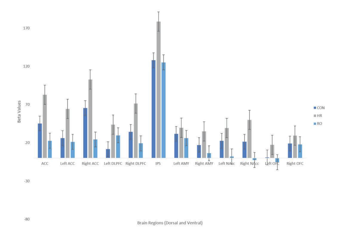
The behavioral and fMRI findings provide insights into working memory and emotional regulation deficits in patients with genetic high risk and recent-onset schizophrenia. Our behavioral results show that patients with RO Schizophrenia and participants in the HR group did not exhibit a significant change in task performance between the Neutral and Negative conditions, while the control participants did. Imaging results of controls are consistent with other studies and show activation in Dorsal and Ventral regions. These results support the belief that the dorsal and ventral regions chosen for this study are activated during WM and emotional regulation tasks.

Our results may show the effects of emotional blunting in RO participants, since in the Neutral > Negative condition, for all ventral regions, RO did not exhibit significant differences. Emotional blunting may cause this, as RO participants are less impacted by the valence of the task and redirect capacity to other functions, such as working memory. This is reflected in their performance results as well, with the least change in D′ from Neutral to Negative, even if overall performance is worse. Increased activation in WM regions was linked with better performance in participants. The D′ values reflect this, as HR consistently had higher activation than Controls and RO and also performed better in the task.

When looking at the activation in the Neutral condition between groups, we observed significant abnormal deactivation/lower activation in ACC, Left ACC, Right ACC, Left DLPFC and Left NAcc. In previous studies, schizophrenic patients often have diminished activation when compared to controls [3]. In looking at ventral regions, the underactivation of the Amygdala in patients with schizophrenia in response to negative stimuli may not be due to underactivation in the Negative condition, but due to overactivation in response to neutral stimuli [3]. These findings reflect the emotional experience reported by people with schizophrenia, where they often experience more negative emotions in response to neutral stimuli [3]. Previous studies show that other brain regions also showed less activation, such as the ACC and DLPFC [3], which our results reflect.

We also observed that HR participants showed consistent overactivation in dorsal and ventral regions compared to control participants for both the Neutral and Negative conditions, which was surprising. Based on previous studies, we expected HR to show levels of cognitive performance intermediate between healthy controls and schizophrenic patients [13]. Even though HR activation tended to be more similar to control activation in scale, it was always greater than Control and RO activation. One possible interpretation is that HR participants are suffering from WM and emotional processing deficits, so the activation is greater in order to compensate for these deficits; RO may just have less activation overall due to task tunneling and having a lower capacity to spend on both WM and emoFigure 7. Significant links between D′ and Activa-

tion.

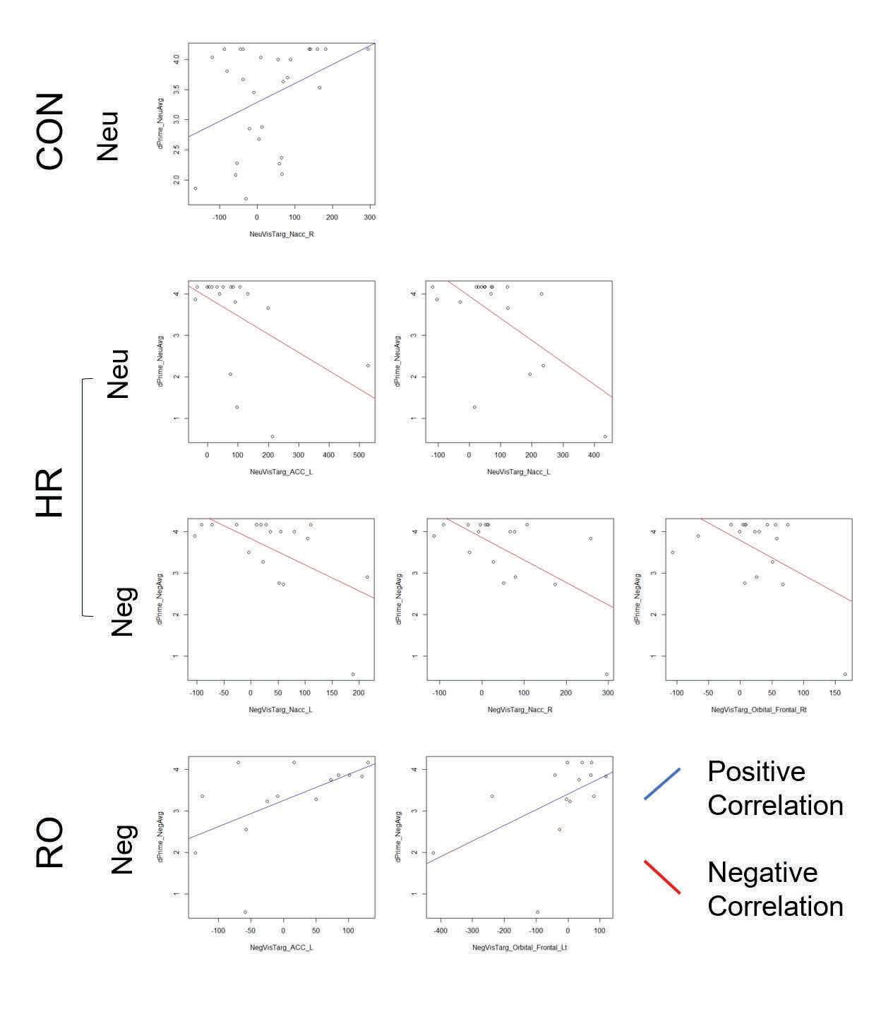
tional regulation.

Interestingly, our results suggest that during an effortful cognitive task, less brain activity was associated with a significant reduction in CON and RO patients’ performance and more brain activity was associated with a significant reduction in HR participants’ performance. HR exhibited the opposite trend compared to RO and Control participants when examining brain activation and task performance. Further connectivity analysis could help us gain a better understanding of why this occurs.

This study has several limitations. First, the sample size of the participant groups (Con, HR, RO) was relatively small and there were significant differences regarding participant age and gender between groups, which may limit the interpretability of the results. Secondly, only Neutral, Negative, and Neutral > Negative conditions of the task were considered. By utilizing the positive conditions and other brain circuits, we might be able to provide more information about the differences between groups during an emotional one-back task. There was no co-variate included for medication in the RO group, which may affect our results. Finally, the behavioral results were only for a subset of participants, which may limit the interpretability of the D′ values and the linkage with performance.

In the future, we hope to utilize these results in patient diagnosis and patient outcome. We also hope to explore the interplay of symptoms of schizophrenia with WM and emotional regulation and include different neural circuits based on the regions involved.

In summary, by using an emotional one-back task allowing for the analysis of the interplay of WM and ER, we demonstrated between-group differences attributed to emotional blunting and surprising results for highrisk participants. Our findings indicate that RO patients tend to show deactivation/lesser activation in WM and ER regions, which can be attributed to limited capacity (and less activation overall), with fewer changes due to emotional valence. Interestingly, our results suggest that during an effortful cognitive memory task with no emotional valence, HR does not fall between CON and SZ as an intermediate, but instead exhibits greater activation. Another surprising finding of HR was that less brain activity was associated with a significant reduction in CON and RO patients’ performance, while more brain activity was associated with a significant reduction in HR participants’ performance. Understanding the WM and emotional processing deficits in schizophrenia is a critical target for improving diagnosis and recovery outcomes in schizophrenia.

6. Acknowledgments

I would like to acknowledge Dr. Andrea Pelletier-Baldelli, Dr. Aysenil Belger and Mr. Josh Bizzell from the UNC Department of Psychiatry for their help with understanding the cognitive side of this project, as well as providing the data used here, Mr. Robert Gotwals for his guidance during the research process, and the Research in Computational Sciences Program at NCSSM.

7. References

[1] Guimond, S., Padani, S., Lutz, O., Eack, S., Thermenos, H., & Keshavan, M. (2018). Impaired regulation of emotional distractors during working memory load in schizophrenia. Journal of psychiatric research, 101, 14–20.

[2] Seidman, L. J., Thermenos, H. W., Poldrack, R. A., Peace, N. K., Koch, J. K., Faraone, S. V., & Tsuang, M. T. (2006). Altered brain activation in dorsolateral prefrontal cortex in adolescents and young adults at genetic risk for schizophrenia: An fmri study of working memory. Schizophrenia research, 85(1-3), 58–72.

[3] Kring, A. M. [Ann M], & Elis, O. (2013). Emotion deficits in people with schizophrenia. Annual review of clinical psychology, 9, 409–433.

[4] Becerril, K., & Barch, D. (2011). Influence of Emotional Processing on Working Memory in Schizophrenia. Schizophrenia Bulletin, 37(5), 1027–1038. doi:10.1093/schbul/ sbq009 [5] Forbes, N., Carrick, L., McIntosh, A., & Lawrie, S. (2009). Working memory in schizophrenia: A meta-analysis. Psychological medicine, 39(6), 889–905.

[6] Eryilmaz, H., Tanner, A. S., et al. (2016). Disrupted Working Memory Circuitry in Schizophrenia: Disentangling fMRI Markers of Core Pathology vs Other Aspects of Impaired Performance. Neuropsychopharmacology, 41(9), 2411–2420. doi:10.1038/npp.2016.55

[7] Gray, J. R., Braver, T. S., & Raichle, M. E. (2002). Integration of emotion and cognition in the lateral prefrontal cortex. Proceedings of the National Academy of Sciences, 99(6), 4115–4120.

[8] Lang, P. J., Bradley, M. M., Cuthbert, B. N., et al. (1999). International affective picture system (iaps): Instruction manual and affective ratings. The Center for Research in Psychophysiology, University of Florida.

[9] Kring, A. M. [A. M.], & Moran, E. K. (2008). Emotional Response Deficits in Schizophrenia: Insights From Affective Science. Schizophrenia Bulletin, 34(5), 819–834. doi:10.1093/schbul/sbn071

[10] Jenkinson, M., Bannister, P., Brady, M., & Smith, S. (2002). Improved optimization for the robust and accurate linear registration and motion correction of brain images. Neuroimage, 17(2), 825–841.

[11] Smith, S. M., Jenkinson, M., et al. (2004). Advances in functional and structural mr image analysis and implementation as fsl. Neuroimage, 23, S208–S219.

[12] Thomas Yeo, B., Krienen, F. M., et al. (2011). The organization of the human cerebral cortex estimated by intrinsic functional connectivity. Journal of neurophysiology, 106(3), 1125–1165.

[13] Bang, M., Kim, K. R., Song, Y. Y., Baek, S., Lee, E., & An, S. K. (2015). Neurocognitive impairments in individuals at ultra-high risk for psychosis: Who will really convert? Australian & New Zealand Journal of Psychiatry, 49(5), 462–470.

SESAMOL AS A NOVEL REDOX MEDIATOR FOR THE ELECTROCHEMICAL SEPARATION OF CARBON DIOXIDE FROM FLUE GAS

Madison Houck

Abstract

The increasing presence of carbon dioxide in the atmosphere has contributed to overall rising temperatures over the past several years. In particular, flue gas, which contains a mixture of carbon dioxide, nitrogen, and oxygen, is a common way that large quantities of carbon dioxide are introduced to the atmosphere. Previously, the redox couple hydroquinone and benzoquinone were applied to a fuel cell capable of separating carbon dioxide from other gases, but the negative environmental impacts of these chemicals have prompted a search for an environmentally friendly option. This project seeks to apply the proton-coupled electron transfer (PCET) reaction of sesamol to achieve the same effect. Cyclic voltammetry was used to evaluate the electrochemical response of sesamol. Cyclic voltammograms show that sesamol undergoes a quasi-reversible reaction in sodium bicarbonate, with peaks that correspond to a redox couple appearing after one cycle or after a deposition. Additionally, half-cell liquid phase testing was performed, confirming that sesamol’s redox reaction creates a pH gradient that drives carbon dioxide to be released at the anode. Furthermore, the construction of a fuel cell reveals that with applied voltage, carbon dioxide concentration increases on the permeate side of the cell when sesamol is utilized as a redox mediator. Future work can be done to further evaluate the efficiency of a sesamol fuel cell as compared to a quinone fuel cell, and to confirm that the system selectively transports carbon dioxide, and not other components of flue gas.

1. Introduction

As global temperatures continue to rise as a result of carbon dioxide’s increasing presence in the atmosphere, the wide-reaching impacts of climate change have driven researchers to search for new carbon dioxide remediation techniques [1]. Many have been developed, including the use of metal-organic frameworks, the direct reduction of carbon dioxide, and the use of nucleophiles to bind to carbon dioxide [2]. However, some of these techniques fall short when it comes to practical applications because of the large amounts of carbon dioxide that enter the atmosphere through flue gas. Flue gas is created when fuel or coal is burned, and is composed of oxygen, nitrogen, water vapor, carbon dioxide, and trace amounts of other gases. Many of the carbon dioxide capture technologies mentioned above are rendered useless when exposed to flue gas; oftentimes, water or nitrogen gas interfere with the mechanisms used. Some technologies are simply not selective for carbon dioxide, and some are structurally damaged by the presence of other gases [3].

This problem prompted research into an applicable technology that uses a fuel cell to electrochemically separate carbon dioxide from other gases. These technologies rely on carbon dioxide’s unique sensitivity to pH changes. A pH gradient is established in the fuel cell that captures carbon dioxide, and has no impact on the gases that might be present in the mixture. Such a gradient is established through the use of a redox mediator that undergoes a reversible proton-coupled electron transfer reaction. The

Figure 1. Schematic for a fuel cell capable of separating carbon dioxide from flue gas electrochemically by establishing a pH gradient.

most widely studied redox mediator is a quinone redox couple (shown in Figure 1). Quinones undergo a reversible redox reaction. The reversibility of the reaction is important because it means that the fuel cell can be used repeatedly, an important consideration when considering any wide-scale application. Additionally, the redox reaction that the quinone couple undergoes is a proton-coupled electron transfer reaction (PCET). While electrons are being transferred to oxidize or reduce a species, a proton is also transferred. It is this transfer of protons that drives the pH gradient. As voltage is applied to the fuel cell, the quinone is reduced at the cathode and oxidized at the an-

ode. As it is reduced, protons are consumed, and thus the local pH becomes basic. The basic pH leads to the capture of carbon dioxide as a bicarbonate ion because this capture proves sensitive to subtle pH changes. At the other end of the cell, quinone is reduced, releasing protons, decreasing the pH, and regenerating carbon dioxide gas from bicarbonate ions, that then exits the cell. Carbon dioxide is the only gas that exits; nitrogen, water, or oxygen are not impacted by pH changes and do not cross the cell [3].

Unfortunately, although a quinone couple has been demonstrated to work in a fuel cell to help transfer carbon dioxide across a membrane, it is not a perfect solution. Quinones have negative impacts on the environment and enter largely as air pollutants; since the goal of the fuel cell is environmental remediation, there has been a push to move away from using quinones in practical applications in this technology [4]. Additionally, a species in a common quinone couple, hydroquinone, is a suspected carcinogen [5], prompting a search for a more environmentally friendly option that has similar redox behavior. One compound that has been singled out for its quinone-like properties is sesamol [4]. Isolated from sesame seeds, sesamol is unlikely to have a negative impact on the environment. It is composed of a fused ring structure, and has a hydroxyl group attached to the benzene ring. Sesamol’s redox mechanism is shown in Figure 2 and is slightly more complex than that of a quinone; the reaction is quasi-reversible. The first step of the reaction is irreversible, but it creates a quinone structure (2-hydroxymethoxybenzoquinone or 2-HMBQ) that then undergoes a second reduction reaction (to form 2-hydroxymethoxyhydroquinone or 2-HMHQ). This second reaction is reversible, and largely mimics a quinone’s redox behavior in that it transfers a proton as well [6].

Figure 2. Scheme proposed for the oxidation of sesamol in aqueous solutions, forming 2-hydroxymethoxybenzoquinone that undergoes further reduction.

This project aims to identify sesamol as a more environmentally friendly alternative to quinones in a fuel cell used for the separation of carbon dioxide from other gases. First, sesamol’s quasi-reversible reaction was studied through cyclic voltammetry in sodium bicarbonate and saturated with both argon and carbon dioxide to examine if conditions present in a fuel cell would fundamentally alter the mechanism of the reaction. Two peaks corresponding to the reversible redox reaction appeared upon repeated sweeps, demonstrating that a reversible reaction begins to occur after an irreversible step. Next, it was confirmed that sesamol undergoes a PCET reaction; this was accomplished through the use of half-cell liquid-phase testing, which saw an increased current and gas evolution when in sodium bicarbonate and saturated with carbon dioxide. Finally, sesamol was used as a redox mediator in a fuel cell and carbon dioxide transport across the cell was achieved.

2. Materials and Methods

2.1 – Materials

The polypropylene membrane, Celgard 3501 was a generous gift from Celgard (Charlotte, NC). The Toray Carbon Paper 060 electrode was purchased from The Fuel Cell Store. Gases were industrial grade purchased from Airgas. All other chemicals were purchased from Sigma-Aldrich, and used without further purification.

2.2 – Cyclic Voltammetry

Cyclic voltammetry was performed on 10 mM 2,6-dimethylhydroquinone, 10mM 2,6-dimethylbenzoquinone, and 1mM sesamol with 0.5 M sodium bicarbonate as the analyte solution using an eDAQ potentiostat (ER466) and a three electrode arrangement. The concentration of sesamol was decreased in order to better examine each peak that appeared. Each trial was performed in a 4 mL conical vial. The reference electrode was silver/silver chloride, the counter electrode was platinum/titanium, and the working electrode was glassy carbon. The working electrode was polished with a 0.3μM alumina suspension, and then rinsed with acetone and water. The reference and counter electrodes were rinsed with acetone and water. The electrodes were all cleaned between each trial. Solutions that were saturated with gas underwent 10 minutes of gas sparging with argon gas, and then 10 more minutes of sparging with carbon dioxide gas, as necessary. The pH of each sample was measured with a Vernier pH Probe. Each trial consisted of three sweeps in total, measuring the continued electrochemical response of each sample. The scan rate was 100mV/s for each trial, and data were collected from -1.0V to 1.5V.

2.3 – Half Cell Liquid Phase Testing

Half-cell testing was performed in a 4 mL conical vial. The working electrode was a 1cm by 3cm Toray Carbon Paper 060 electrode (Fuel Cell Store), the reference electrode was silver/silver chloride, and the counter electrode was platinum. The carbon paper electrode was rinsed with acetone and water between each trial, as were the counter and reference electrodes. The catalyst was added from a 10mg/mL solution of 20% wt. platinum on carbon black in methanol, which was drop-casted onto the carbon pa-

per electrode at a concentration of 10μL/cm2 and allowed to evaporate. A voltage of 0.5V was applied using eDAQ Chart software. Each solution was tested at a concentration of 100mM in 0.5M sodium bicarbonate or 0.5M sodium sulfate.

2.4 –Fuel Cell Construction

To construct the fuel cell, first a polypropylene membrane (Celgard 3501) was soaked in a solution mixture of 5mM 2,6-DMBQ and 5mM 2,6-DMHQ or 5mM 2-HMBQ and 5mM 2-HMHQ for 24 hours. Sesamol was oxidized electrochemically by applying a voltage of 900mV for 60 seconds to the entire sample, then taking half of that sample by volume and applying a voltage of 400mV for an additional 60 seconds [6]. Two carbon paper electrodes were cut to 25cm2 and placed on either side of the membrane, with the catalyst layer facing the membrane. The catalyst was added from 10uL/cm2 of a 50mg/mL solution of 20% wt. platinum on carbon black in methanol. The membrane electrode assembly was applied to a fuel cell, and efficiency was evaluated using fourier-transform infrared spectroscopy. The permeate side of the fuel cell was attached to the FTIR. Carbon dioxide was flowed into the fuel cell at a rate of 5 standard cubic centimeters (SCCM) per minute, with the sweep gas (argon) at a high flow rate, preventing the CO2 from crossing the membrane. Then, after 10 minutes, once the fuel cell was saturated, the CO2 was turned off and the argon flow rate was decreased significantly. An FTIR scan was taken with no additional voltage applied to measure how much carbon dioxide was diffusing across the membrane initially. Then, a voltage of 2.5 V was applied with a voltmeter and FTIR scans were taken after 1, 5, and 10 minutes. The voltage was then turned off for 5 minutes and another FTIR scan was taken to examine if CO2 was simply leaking across the fuel cell over time.

3. Results

3.1 – Cyclic Voltammetry

Figure 3. Cyclic voltammogram of 2,6-DMHQ in .5M sodium bicarbonate.

The redox reaction of 2,6-dimethylhydroquinone has been well studied because of its reversibility [4]. It has a clear oxidation peak (at 0V) and reduction peak (at -0.2V). The reaction proceeds this way under argon and carbon dioxide saturated conditions. Upon repeated scans, the shape of the voltammogram does not change appreciably.

a)

b)

c)

Figure 4. Cyclic voltammograms for sesamol in 0.5M acetic acid with (a) no gas saturation (oxidation steps labelled), (b) argon gas saturation, and (c) carbon dioxide gas saturation.

Cyclic voltammetry was also used to characterize sesamol’s redox reaction. The quasi-reversible scheme proposed by Brito et al. is supported by the appearance of secondary peaks referred to as “shoulder peaks” after one voltage cycle (Fig. 4a). The oxidation peak that initially appears around 0.7V represents the irreversible step that creates 2-HMBQ. After this species is present, the reduction peak at 0V corresponds to the creation of 2-HMHQ which

is then oxidized. This oxidation peak, one of the shoulder peaks, is noticeable in the next scan. This occurs around 0.4V. Additionally, after the shoulder peak appears, the shape remains the same upon repeated scans, indicating a continued and predictable electrochemical response. Under argon saturated conditions, the voltammograms appear similar. Additionally, when the sample was purged with argon and then saturated with carbon dioxide, the voltammogram shape remains consistent. Past a potential of 1V, the aqueous solution begins to oxidize, thus the pertinent data remain between -1V and 1V on the voltammogram.

a)

b)

c)

Figure 5. Cyclic voltammograms of 1mM sesamol in .5M sodium bicarbonate with (a) no gas saturation, (b) argon gas saturation, and (c) carbon dioxide gas saturation.

The redox mechanism of sesamol was next examined in a solution of sodium bicarbonate instead of acetic acid (Fig. 5). The sodium bicarbonate solution yields a much higher pH (9.52 instead of 2.49), which could be important to consider in the mechanism of sesamol oxidation, as it is assumed that both protons and electrons are transferred. There is less peak definition in the sodium bicarbonate; however, despite this, shoulder peaks can still be observed, albeit at slightly different potentials. Here, the irreversible oxidation step likely occurs between 0.3V and 0.4V, and the shoulder peak first appears around 0.1V. There is the slight appearance of a reduction peak around -0.4V which corresponds to the reduction of the 2-HMBQ. Under argon and carbon dioxide conditions, the general shape of the voltammogram is retained.

3.2 – Half Cell Liquid Phase Testing

Half-cell liquid phase testing was performed on samples of hydroquinone and sesamol (Fig. 6). When potentials were applied, the current was measured and the sample

a)

0.5 M NaHCO3

0.5 M NaHCO3 no no

yes yes

b)

0.5 M Na2SO4 no no

0.5 M Na2SO4

c)

0.5 M NaHCO3

0.5 M NaHCO3 yes no

no no

yes yes

d)

0.5 M Na2SO4 no no

0.5 M Na2SO4 yes no

Figure 6. Data compiled from half-cell testing on (a) 100mM 2,6-DMHQ and (c) 100mM sesamol. Photograph of carbon paper electrode after half-cell testing was performed on (b) 2,6-DMHQ and (d) sesamol, showing gas evolution.

was observed for the evolution of a gas. When a gas is evolved, it indicates that carbon dioxide is being released at the anode, after the oxidation of the redox mediator and the subsequent release of protons, driving down the local pH. At a lower local pH, carbon dioxide is released from a bicarbonate ion back into its gaseous form and exits the solution. The presence of a gas therefore indicates that the reaction transfers protons as well as electrons; if only

electrons were transferred, the pH would not change and the carbon dioxide would remain in solution. A gas was only evolved when specific conditions were met; firstly, the sample had to have been saturated with carbon dioxide. Secondly, the solvent had to be sodium bicarbonate. A different aqueous solvent, sodium sulfate, was used as a negative control for gas evolution. As expected, gas was evolved in a carbon dioxide saturated solution of 100mM hydroquinone in 0.5M NaHCO3. Additionally, it was found that a 100mM sesamol solution in 0.5 M NaHCO3 also saw gas evolution at the same potential. When each of these redox mediators were in a solution of 0.5M Na2SO4, no gas evolution was seen.

3.3 – Fuel Cell Testing

A fuel cell was tested with no redox mediator, a quinone redox mediator, and a sesamol redox mediator, and relative carbon dioxide concentrations were measured with FTIR.

When the membrane placed in the fuel cell was soaked in a solution of 0.5 M NaHCO3, little to no difference was seen in the relative concentrations of carbon dioxide on the permeate side of the cell even when voltage was applied and subsequently turned off. The carbon dioxide peak was identified to be between 2300 and 2330 cm-1 . The data were baseline shifted to begin at the same transmittance value because the FTIR reported different initial transmittance values with each measurement.

Figure 7. Normalized FTIR spectra of permeate side of a fuel cell with membrane soaked in 0.5 M NaHCO (no redox mediator). Spectra were taken with no 3 voltage applied (blue), with 2.5 V applied after 1 min (orange), after 5 min (gray), after 10 min (yellow) and after the voltage had been turned off for 5 min (light blue).

When the membrane was soaked in 5mM 2,6-DMHQ+ 5mM 2,6-DMBQ, the carbon dioxide peak increased in size as the voltage was applied to the cell for progressively longer amounts of time. The most carbon dioxide was present on the permeate side when a voltage of 2.5V had been applied for 10 minutes, as represented by the yellow peak in Figure 8.

Figure 8. FTIR spectra of permeate side of a fuel cell with membrane soaked in 5mM 2,6-DMHQ+ 5mM 2,6DMBQ in .5 M NaHCO . Spectra were taken with no 3 voltage applied (blue), with 2.5V applied after 1 min (orange), after 5 min (gray), and after 10 min (yellow).

When the membrane was soaked in a sesamol solution that had been oxidized electrochemically to form 5mM 2-HMBQ + 5mM 2-HMHQ, a similar carbon dioxide increase was seen over time (Fig. 9). The largest peak was seen when the fuel cell had been running for ten minutes. Additionally, when the voltage was turned off for 5 minutes, the concentration of carbon dioxide decreased again, above any peak that occured when voltage had been applied.

Figure 9. FTIR spectra of permeate side of a fuel cell with membrane soaked in 5mM 2-HMBQ + 5mM 2-HMHQ (generated from the oxidation of sesamol) in .5 M NaHCO . Spectra were taken with no voltage 3 applied (orange), with 2.5 V applied after 1 min (gray), after 5 min (yellow), after 10 min (blue) and after the voltage had been turned off for 5 min (green).

The sesamol fuel cell saw the greatest increase in peak height over the ten minutes voltage was applied (Fig. 10). Although this does not directly correlate to an increase in fuel cell function, since FTIR testing cannot quantify efficiency, it does indicate that sesamol is a functional redox mediator that is qualitatively on par with quinone.

Figure 10. Graph representing peak height vs. time the voltage has been applied measured from the initial peak height. Compiled data from bicarbonate fuel cell (green), quinone fuel cell (blue), and sesamol fuel cell (yellow).

4. Discussion

The cyclic voltammograms of sesamol above (Fig. 4 and 5) support the proposed scheme for the oxidation of sesamol, which involves the creation of a quinone species. The presence of shoulder peaks points to the creation of a new compound (2-hydroxymethoxybenzoquinone) in the first step of the reaction, and the subsequent reversible reaction these compound(s) undergo. When the sample is purged with argon, (Fig. 4b and 5b), none of the voltammograms change shape dramatically, suggesting that none of the peaks were due to the presence of oxygen in the sample. Additionally, carbon dioxide does not interfere with the progression of the reaction, as when the samples are purged with carbon dioxide, the voltammograms retain their general shape (Fig. 4c and 5c). Although the cyclic voltammograms in bicarbonate have less defined peaks (see Fig. 3), this may be attributed in part to the increased pH and in part to the drift that Ag/AgCl reference electrodes undergo as they age. Further research could be done into the impact of pH on sesamol’s redox reaction to determine if the movement of the peaks represents the impact of an increased concentration of OH- ions available, as these are required for the first irreversible oxidation step of the reaction, and decreased concentration of H+ ions available, as these are required for the reduction of 2-HMBQ to 2-HMHQ. By examining how the pH impacts the progression of the redox reaction, the optimal pH of a fuel cell could be determined for maximum carbon dioxide transport [3].

Half-cell testing results fully support the hypothesis that sesamol undergoes a proton-coupled electron transfer reaction because in sodium bicarbonate, a carbon dioxide saturated solution saw gas evolution at a 0.5V potential. This gas evolution would not be possible without the transfer of protons creating an acidic pH at the anode, subsequently driving the release of carbon dioxide dissolved in solution as a gas, observed on the electrode. It is important to note that since only a 0.5V potential was applied, none of the gas evolution would be expected to be due to water-splitting [7]. Additionally, the platinum catalyst was chosen because it does not contribute heavily to water-splitting, even at higher potentials [3].

Fuel cell testing suggests that quinone and sesamol redox mediators, rather than the simple application of voltage, are responsible for moving carbon dioxide across the fuel cell. Additionally, the decrease in concentration observed when the voltage is removed dispels the theory that carbon dioxide is leaking over to the permeate side of the cell over time. Further work is necessary to evaluate the efficiency of each fuel cell, as this project’s set-up was not equipped to evaluate percent carbon dioxide transported, only observe relative decreases or increases in concentration. Plotting peak height against time reveals that sesamol and quinone have similar efficiencies in this setting. All evidence of carbon dioxide transport was qualitative. Percent carbon dioxide efficiency can be evaluated with different applied potentials as well, not just 2.5V. Further research can also be done to verify that the mechanism is selective for carbon dioxide by pumping a mixture of nitrogen, oxygen and carbon dioxide, rather than pure carbon dioxide, across a fuel cell to further emulate flue gas conditions. One area of concern is that the platinum catalyst will catalyze water-splitting and that oxygen could be released on the permeate side with carbon dioxide, although previous works have found that platinum on carbon black does not generate oxygen in large amounts as other similar metal catalysts might [3].

5. Conclusion and Future Work

It has been shown that sesamol undergoes a quasi-reversible redox reaction in sodium bicarbonate; it is assumed that two non-toxic quinones are created, 2-hydroxymethoxybenzoquinone and 2-hyroxymethoxyhydroquinone, that further reduce and oxidize reversibly while transfering protons. The appearance of shoulder peaks in the cyclic voltammograms supports this reaction scheme, and their relative size and placement indicate that such a reaction is reversible and repeatable. Through half-cell testing, it was confirmed that protons are transferred, thus creating an in situ pH gradient that releases carbon dioxide that has been dissolved in solution at the anode. Based on the results of preliminary fuel cell testing, it can be concluded that sesamol’s quasi-reversible proton-coupled electron transfer reaction functions to transport carbon dioxide across a fuel cell like that of a quinone, and can be used as a more environmentally-friendly choice of mediator to separate CO2 from flue gas.

6. Acknowledgments

The author would like to thank the North Carolina School of Science and Mathematics (NCSSM) Science Department, the NCSSM Foundation, the NCSSM Summer

Research and Innovation Program and research mentor Dr. Michael Bruno. Additionally, this research would not have been possible without the generous gift of polypropylene membrane from Celgard (Charlotte, NC).

7. References

[1] Wuebbles, D. (2017). USGCRP: Climate Science Special Report: Fourth National Climate Assessment, Volume I. U.S. Global Change Research Program. DOI: 10.7930/ J0J964J6.

[2] Rheinhardt, J. (2017). Electrochemical Capture and Release of Carbon Dioxide. ACS Energy Letters 2 (2), 454461 DOI: 10.1021/acsenergylett.6b00608

[3] Watkins, D. (2015). Redox-Mediated Separation of Carbon Dioxide from Flue Gas. Energy & Fuels 29 (11), 7508-7515 DOI: 10.1021/acs.energyfuels.5b01807

[4] Gandhi, M. (2018). In Situ Immobilized Sesamol-Quinone/Carbon Nanoblack-Based Electrochemical Redox Platform for Efficient Bioelectrocatalytic and Immunosensor Applications. ACS Omega 3 (9), 10823-10835 DOI: 10.1021/acsomega.8b01296

[5] Bolton, J (2017). Formation and Biological Targets of Quinones: Cytotoxic versus Cytoprotective Effects. Chemical Research in Toxicology 30 (1), 13-37, DOI: 10.1021/ acs.chemrestox.6b00256

[6] Brito, R. (2014). Elucidation of the Electrochemical Oxidation Mechanism of the Antioxidant Sesamol on a Glassy Carbon Electrode. Journal of the Electrochemical Society 161 (5), 27-32, DOI: 10.1149/2.028405jes

[7] Stretton, T. (n.d.). Standard Reduction Table. Retrieved November 13, 2019, from http://www2.ucdsb.on.ca/tiss/ stretton/Database/Standard_Reduction_Potentials.htm.

MODELING THE EFFECT OF CHEMICALLY MODIFIED NON-ANTIBIOTIC TETRACYCLINES WITH β-AMYLOID FIBRILS TO TREAT ALZHEIMER’S DISEASE

Rachel Qu

Abstract

Alzheimer’s Disease is a neurodegenerative disorder in which memory and comprehensive abilities are lost over time. There is currently no known cure, but the disease has been linked to the aggregation of extracellular β-amyloid plaques. The tetracycline family of antibiotics has been shown to reduce plaque formation, but use in more complex treatments involves the risk of bacterial resistance. This project explores the use of tetracycline’s non-antibiotic analogs to reduce β-amyloid aggregation. Certain chemically modified non-antibiotic tetracyclines (CMTs) were selected to be modeled alongside the known β-amyloid aggregation inhibitors tetracycline, doxycycline, and minocycline. These were then analyzed computationally using Molegro to predict the binding affinities of certain CMTs to the β-amyloid protein fibril. CMT-3 (6-deoxy-6-demethyl-4-dedimethylamino tetracycline), CMT-4 (7-chloro-4-dedimethylamino tetracycline), CMT-5 (tetracycline pyrazole), and CMT-7 (12-deoxy-4-dedimethylamino tetracycline) were seen to bind more effectively than known inhibitors. The same compounds were then analyzed using StarDrop, helping to determine how effective the compounds could perform as oral drugs, and CMT-3 and CMT-7 were suggested to be more suitable in acting as oral drugs. This information was then used in studies with transgenic Caenorhabditis elegans to confirm results. Treatment in more complex models, like vertebrates, could be applied in the future to develop a novel treatment method for Alzheimer’s Disease.

1. Introduction

1.1 – Alzheimer's Disease

Alzheimer’s Disease (AD), the most common type of dementia, is a neurodegenerative disorder in which memory and comprehensive abilities are slowly lost over time [1]. Most symptoms appear in more elderly individuals, with symptoms generally appearing after age 60 [2]. Features of the disease include the loss of connections between neurons. Damage appears to initially take place in the hippocampus, spreading outward as progression occurs [3]. By 2060, the number of Americans with the disease is projected to hit around 14 million. Currently, effective prevention methods do not exist, as there is no known cure for Alzheimer’s [2]. This is detrimental because AD is one of the highest ranking causes of death in the United States.

AD occurs when brain cells that typically process, store, and retrieve information degenerate and die [4]. There are two supposed causes for this disease, traced back to β-amyloid (Aβ) peptides and tau proteins. The accumulation of intracellular neurofibrillary tangles (NFTs), composed of tau proteins, used to stabilize microtubules when phosphorylated, is associated with AD. In addition, extracellular plaques are also exhibited in patients with AD. Aβ peptides, created from the breakdown of amyloid precursor protein (APP) primarily form these plaques [5]. The amyloid hypothesis assumes that mistakes in the process governing the production, accumulation, and/or disposal of Aβ proteins are the primary cause of AD. These proteins accumulate in the brain, disrupting communication between brain cells and killing them.

1.2 – β-Amyloid Fibrils

Amyloid precursor protein (APP) is cut by other proteins into smaller separate sections. One of these sections becomes Aβ proteins, which tend to accumulate. It is currently believed that small, soluble aggregates of Aβ are more toxic [4]. First, they form small clusters, or oligomers, and then chains of clusters called fibrils. The fibrils then form mats called β-sheets. Finally, the mats come together to form the plaques seen in AD [4]. Because the cleavage process by γ-secretase that forms Aβ is not always entirely precise, Aβ peptides of different lengths can be formed [6]. Aβ-42 is one of these, thought to be especially toxic [3].

Because Aβ production and its subsequent fibril formation is assumed to be a cause of AD, inhibiting Aβ aggregation could lead to a potential cure for AD. Since Aβ’s structure relies on hydrogen bonds for β-sheet mat formation, disruption by certain compounds can potentially be used to prevent aggregation. The alternating hydrogen bond donor-acceptor pattern has been thought to be complementary to the β-sheet conformation of Aβ-42 [7]. Previous compounds known to act as alleviants or deterrents of AD have been seen to contain certain common features that suggest the hydrogen bonds donor-acceptor-donor patterns are responsible for interrupting the β-sheet formation of Aβs [7].

1.3 – Tetracycline and CMTs

Even though there is no definitive cure, there are still treatment options that exist to alleviate AD. Many are natural products with medicinal properties, but other options also exist. Some compounds like aged garlic extract, curcumin, melatonin, resveratrol, Ginkgo biloba extract, green tea, and vitamins C and E have been tested in Alzheimer’s patients and show promise [8-9]. Tetracycline and its analogs like doxycycline and minocycline have also been shown to do the same [10].

Observing tetracycline and some of its analogs showed similarities in structure between the three compounds. These specifically included a pattern of alternating hydrogen bond donors and acceptors attached to adjacent rings on all three compounds. It was hypothesized that this alternating donor-acceptor-donor pattern had some basis in affecting Aβ fibrils, since tetracyclines have been shown to dissolve these structures after formation [10]. This was based on the fact that hydrogen bond interactions hold the β-sheet’s pleated sheet structure together. Since the donor-acceptor-donor pattern mimics the patterns in the sheet, it is possible that structures like tetracyclines can disrupt this hydrogen bonding and thus the structure of the sheet itself. By disrupting hydrogen bonds in β-sheets, the protein no longer retains its shape and theoretically loses its original structure. By this basis, the fibril formation would be disrupted or reversed and Aβ would not be able to continue to form its characteristic plaques.

Though tetracycline, doxycycline, and minocycline have been shown to be effective, they all exhibit antibacterial characteristics [10]. Antibiotic activity is linked to the presence of the dimethylamine group present on the structure (Fig. 1). This could lead to poor side effects, specifically bacterial antibiotic resistance, if clinically used to treat AD. Removal of this group while maintaining the primary structure of the donor-acceptor-donor pattern would ideally lead to the formation of an improved AD drug.

Chemically modified non-antibiotic tetracyclines (CMTs) have been synthesized and can be applied to Aβ aggregation inhibition. They have similar structures to tetracycline but remove the dimethylamine group responsible for antibiotic properties. Since studies have shown that tetracycline and its analogs can be effective through preventing and inhibiting Aβ aggregation, the possible use of CMTs that still contain the alternating H-bond donor/ acceptor pattern but do not have antibiotic properties is of interest.

1.4 – Hypothesis/Goals

It is hypothesized that the treatment of AD can be approached through the use of CMTs to reduce Aβ aggregation, which can be modeled both computationally and in vivo through the use of Caenorhabditis elegans. The goals of this project were to first computationally model Aβ interactions with different compounds using Molegro to evaluate aggregation inhibition efficiency, and then evaluate the same compounds for effectiveness as oral drugs in StarDrop. After computational modeling, selected compounds were to be used with a transgenic version of the model organism C. elegans to test the in vivo effects of selected compounds through a paralysis assay.

Figure 1. Structure of tetracycline indicating alternating hydrogen bond donor-acceptor-donor pattern (circled in red) and dimethylamine group (squared in blue).

2. Materials and Methods

Molegro Virtual Docker and Molegro Data Modeller were used to analyze the binding affinity of multiple chemically modified tetracyclines (CMT-1, CMT-3, CMT-4, CMT-5, CMT-6, CMT-7, CMT-8) to Aβ proteins. Aβ structure 2MXU was taken from the Protein Data Bank. CMT structures were created in ChemDraw and translated to PDB files by putting the SMILES code through an online translator. After docking CMT structures, their Ligand Rerank scores were converted to binding affinity scores using Molegro’s Binding Affinity algorithm. StarDrop was used to analyze the ability of the drug to reach the target cells using Lipinski’s Rule of Five and an Oral CNS scoring profile. Data from Molegro and StarDrop were taken into account to rank the drug performance and narrow the list of potential drugs.

CL2006 strain of Caenorhabditis elegans was obtained from the Caenorhabditis Genetics Center at the University of Minnesota and grown on Nematode Growth Medium plates. CMT-3 was purchased from Echelon BioSciences. All other chemicals were obtained from Sigma Aldrich and dissolved in water before use.

C. elegans were propagated at 15 degrees Celsius on solid Nematode Growth Medium (NGM). Age synchronization was performed by picking worms of the same life stage, L1s, and plated on plates seeded with tet-resistant zim-2 Escheria coli. After 48 hours, plates were treated with 100 μL of vehicle or drugs (100 μM each). After 24 hours, the temperature was raised to 24 degrees Celsius and paralysis was scored until 120 hours of age. Paralysis was evaluated

by touching the worms’ heads; paralysis was scored if the worm did not move or only moved the head.

3. Results/Discussion

3.1 – Molecular Docking Studies

Molegro is a computational platform for predicting protein-ligand interactions. In Molegro, the protein 2MXU was taken from the Protein Data Bank as a model of Aβ fibril aggregation. 2MXU shows a fibril structure composed of multiple peptide monomers. Two different approaches were taken with this protein. One was of a smaller fibril structure and the other of a dimer with a cavity located between. Because the mechanism behind how drugs like tetracycline work to dissolve the preformed fibril is not currently known, both approaches were used. With the fibril structure approach, the ligand bonds to the outside of the fibril protein in a smaller cavity. With the dimer structure approach, the ligand binds between the two monomers (Fig. 2).

Figure 2. Molegro screencap of Aβ fibril protein 2MXU with tetracycline (green) integrated into both fibril structures (top) and dimer structure (bottom).

When modeling the effectiveness of different ligands on Aβ aggregation inhibition efficiency, tetracycline and its analogs can be interpreted as effective through the analysis of binding affinities. Binding affinities show more effective binding when more negative. Through using Molegro to model the interactions between protein and ligand, it was possible to find that in both the fibril and dimer formation, CMTs repeatedly and consistently outperform tetracycline and its natural analogs (Tab. 1).

Table 1. Molegro data table of binding affinities, where more negative values are more effective, for tetracycline and analogs with both the fibril (top) and dimer (bottom) approaches.

Tetracycline -9.69 Doxycycline -10.10 Minocycline -8.28

CMT-3 -14.43 CMT-1 -13.45

Tetracycline -11.00 Doxycycline -12.33 Minocycline -9.37 CMT-3 -17.17

Among the CMTs themselves, however, there were varied results. By testing different CMTs, it was possible to find the more effective Aβ aggregation inhibitor to use in further treatment. CMTs-1, 3, 4, 5, 6, 7, and 8 were all used (Fig. 3). Because the same trend was seen in both the fibril and dimer approach, with CMTs outperforming tetracycline and its natural analogs, the calculated binding affinities were only compared for the fibril approach. The compounds with the most effective binding affinities were shown to be CMT-3, CMT-4, CMT-5, and CMT-7 (Tab. 2).

Figure 3. Structures of CMTs (in order: 1, 3, 4, 5, 6, 7, 8).

Table 2: Molegro data table of binding affinities for CMT's using the fibril approach

Molecule

CMT-1 (4-dedimethylaminotetracycline) CMT-3 (6-deoxy-6-demethyl-4-dedimethylaminotetracycline)

Binding affinity (average)

-13.45

-14.43

CMT-4 (7-chloro-4-de-dimethylamino tetracycline) -17.03

CMT-5 (tetracycline pyrazole) -16.01 CMT-6 (4-dedimethylamino. -11.32 4-hydroxytetracycline) CMT-7 (12-deoxy-4-de-dime- -15.26 thylamino tetracycline) CMT-8 (4-dedimethylaminodox- -14.09 ycycline)

3.2 – Drug Efficiency Analysis

StarDrop was used in determining how the different CMTs would perform as oral drugs in treating AD. Lipinski’s Rule of Five and an Oral Central Nervous System (CNS) Profile were both performed. Lipinski’s Rule of Five evaluates if a compound will be a likely active drug in humans. The criteria include a maximum value of 5 for octanol-water partition coefficient (logP) which measures hydrophobicity, a maximum of 500 Da molecular weight (MW), a maximum of 5 hydrogen bond donors (HBD) and 10 hydrogen bond acceptors (HBA). It was shown that CMT-3 and CMT-7 were the only two CMTs that fulfilled all four criteria, with even tetracycline and doxycycline only meeting three of the four requirements (Tab. 3). Since tetracycline, doxycycline, and minocycline are all used in practice as drugs, Lipinski’s Rule of Five is only one guideline for drug design and not absolutely required for effective drugs. However, it can still be used as a guideline to corroborate the potential effectiveness of CMT-3 and CMT-7.

An Oral CNS profile was also performed using StarDrop. Because AD is related to the brain, the drugs need to be able to be analyzed in the context of the central nervous system. While none of the compounds exhibited ideal Oral CNS profiles, many outperformed tetracycline. Since tetracycline is known to be able to be used in the context of treating the brain [10], the criteria used for a drug to be deemed effective was an Oral CNS Profile score higher than that of tetracycline. This allowed CMT-3, 4, 5, 7, and 8 to all be predicted as effective Oral CNS drugs (Tab. 4).

From the results of StarDrop and Molegro combined, it was determined that CMT-3 and CMT-7 were the best candidates for binding to the fibril and for being an effective drug capable of treating AD through the context of Aβ aggregation. This information was then applied to experi-

Table 3: StarDrop data table of CMTs, tetracycline, doxycycline, and minocycline through the analysis of Lipinski’s Rule of Five. The color scale ranges from green to red, with darker greens being indicators of more effective drugs, and darker reds being indicators of less effective drugs.

0.5 tetracycline -0.8803 444.4 6 10 0.5 doxycycline -0.2456 444.4 6 10 1 minocycline 0.4239 457.5 5 10 0.5 CMT-1 -0.3233 401.4 6 9

1 CMT-3 0.7645 371.3 5 8 0.5 CMT-4 0.9379 435.8 6 9

0.5 CMT-5 -0.3333 397.4 6 9

0.5 CMT-6 -0.9992 417.4 7 10

1 CMT-7 0.4774 385.4 5 8 0.5 CMT-8 0.1577 401.4 6 9

3.3 – Caenorhabditis elegans

Caenorhabditis elegans (C. elegans) do not naturally ex-

press Aβ. However, transgenic strains of the nematode exist in which it is possible to model the effectiveness of Alzheimer’s drugs, using temperature-sensitive expression strains. The CL2006 strain of C. elegans, when raised at normal conditions, expresses typical wild-type growth. When shifted to higher temperatures, they conditionally express the Aβ peptide and upon adulthood, paralysis is induced. By treating C. elegans with AD drugs, the percentage of nematodes in which paralysis is expressed will decrease, as Aβ plaques are lessened. The more effective the drug is, the more paralysis should be reduced. Previous studies with tetracycline show that, 48 hours after the temperature shift, around 35 percent of C. elegans treated with doxycycline, minocycline, and tetracycline remained healthy while 100 percent of untreated worms were paralyzed [10].

A similar paralysis assay for the CL2006 strain of C. elegans was performed with CMT-3 and it was found that CMT-3 was more effective at preventing paralysis than tetracycline and doxycycline, with doxycycline being the least effective (Fig. 4).

3.4 – Discussion

Molegro and StarDrop data indicated that the most effective CMTs to treat AD would be CMT-3 and CMT-7, properly known as 6-deoxy-6-demethyl-4-dedimethylamino tetracycline and 12-deoxy-dedimethylamino tetracycline respectively. CMT-3 is commercially available as incyclinide while CMT-7 is not, so CMT-3 was the only CMT taken into consideration in experimental data. In future work, if other CMTs are available, they should also

Table 4. StarDrop data table of CMTs, tetracycline, doxycycline, and minocycline through the analysis of an Oral CNS Scoring Profile. The color scale ranges from green to red, with darker greens being indicators of more effective drugs, and darker reds being indicators of less effective drugs.

0.03053 tetracycline -0.8803 3.002 4.742 2.599 -1.577 - - yes low low 0.08814doxycycline -0.2456 2.833 4.739 2.659 -1.3 - + yes low low 0.1369 minocycline 0.4239 2.591 4.8 3.168 -1.221 - + yes low low 0.02148 CMT-1 -0.3233 1.843 4.91 2.232 -1.217 - - yes low low 0.03198 CMT-3 0.765 1.369 4.833 2.665 -1.094 - - yes lo low 0.06815 CMT-4 0.9379 1.837 5.02 2.371 -1.198 - + yes low low 0.03579 CMT-5 -0.3333 2.412 5.232 2.096 -1.552 - - yes low low 0.01162 CMT-6 -0.9992 2.177 4.971 2.035 -1.3 - - yes low low 0.03813 CMT-7 0.4774 1.556 4.886 2.429 -0.9871 - - yes low low 0.07435 CMT-8 0.1577 1.73 4.88 2.422 -1.206 - + yes low low

be used to measure effectiveness as AD drugs, especially CMT-7.

Figure 4. Paralysis assay of C. elegans paralysis 24 hours after temperature shift to 24 oC.

It has been shown that tetracycline and doxycycline are effective at reducing paralysis in C. elegans [10]. Results shown here support this while suggesting that CMT-3 is also effective at reducing paralysis, potentially even better than the two tetracycline analogs.

However, though data suggest that CMT-3 is overall more effective than tetracycline and doxycycline, the data show large drops and fluctuations during the time period measured, probably due to a smaller sample size in each trial performed. Additionally, there is a 10-hour long time period lost in data collection that distorts the pattern of paralysis as time goes on. In future work, the experimental section should be replicated with a larger sample size and ideally consistent 2-hour intervals throughout the entire approximately 24-hour period, working to confirm the results shown here.

4. Conclusion

It has been concluded through computational analysis that CMTs can be predicted to interact with Aβ in a similar manner to tetracycline and its natural analogs. Especially successful CMTs include CMT-3 and 7, and in vivo trials with model organism C. elegans, specifically temperature-dependent strain CL2006, can model paralysis correlated to Aβ expression. Experimental data shows that CMT-3 does partially recover paralysis in this strain and suggests that other CMTs may do the same.

Tetracycline and its analogs can be used for multiple medicinal applications and can interact with Aβ aggregation in transgenic models of C. elegans to protect them from the paralysis phenotype. Certain CMTs have been computationally modeled to behave in the same manner to a similar and possibly better degree. This is especially applicable to CMT-3 (6-deoxy-6-demethyl-4-dedimethylamino tetracycline) and CMT-7 (12-deoxy-4-dedimethylamino tetracycline) which have been suggested to be better at preventing aggregation with the preformed Aβ fibril and exhibit better interactions as oral drugs. Paralysis assays performed with a transgenic model of C. elegans in an in vivo study seem to exhibit a pattern indicating CMT-3’s ability to prevent paralysis caused by Aβ aggregation and may outperform both tetracycline and doxycycline in its role as an aggregation inhibitor, though future replications must be done to corroborate this phenomenon.

CMT-3 is therefore a promising compound to be used in future studies as a proposed treatment method for preventing or curing AD. It would be done through the same

method tetracycline and its natural analogs exhibit, while still preventing associated bacterial antibiotic resistance, and reducing side effects that would occur in patients through treatment of AD with tetracycline.

5. Acknowledgements

This research was supported by the North Carolina School of Science and Mathematics Science Department, the NCSSM Foundation, and the NCSSM Summer Research and Innovation Program. The author would also like to thank research mentor Dr. Michael Bruno and Dr. Kim Monahan for her assistance in C. elegans research.

6. References

[1] Xu, J., Kochanek, K. D., Sherry, M. A. ;, Murphy, L.,

& Tejada-Vera, B. (2007). National Vital Statistics Reports, Volume 58, Number 19 (05/20/2010). Retrieved from http:// www.cdc.gov/nchs/deaths.htm.

[2] Matthews, K. A., Xu, W., Gaglioti, A. H., Holt, J. B., Croft, J. B., Mack, D., & McGuire, L. C. (2019). Racial and ethnic estimates of Alzheimer’s disease and related dementias in the United States (2015–2060) in adults aged ≥65 years. Alzheimer’s and Dementia, 15(1), 17–24. https:// doi.org/10.1016/j.jalz.2018.06.3063

[3] National Institute on Aging (2017). What Happens to the Brain in Alzheimer's Disease? National Institute on Aging. https://www.nia.nih.gov/health/what-happens-brain-alzheimers-disease

[4] Alzheimer's Association (2017). Beta-amyloid and the amyloid hypothesis. Alzheimer’s Association. https://www. alz.org/national/documents/topicsheet_betaamyloid.pdf

[5] Markaki, M., & Tavernarakis, N. (2010). Modeling human diseases in Caenorhabditis elegans. Biotechnology Journal, 5, 1261–1276. https://doi.org/10.1002/ biot.201000183

[6] Murphy, M. P., & Levine, H. (2010). Alzheimer’s Disease and the Amyloid-β Peptide. Journal of Alzheimer’s Disease, 19(1), 311–323. https://doi.org/10.3233/jad2010-1221

[7] Kroth, H., Ansaloni, A., et al. (2012). Discovery and structure activity relationship of small molecule inhibitors of toxic β-amyloid-42 fibril formation. Journal of Biological Chemistry, 287(41), 34786–34800. https://doi. org/10.1074/jbc.M112.357665

[8] Bui, T. T., & Nguyen, T. H. (2017, September 26). Natural product for the treatment of Alzheimer’s disease. Journal of Basic and Clinical Physiology and Pharmacology, Vol. 28, pp. 413–423. https://doi.org/10.1515/ jbcpp-2016-0147

[9] Wu, Y., Wu, Z., Butko, P., et al. (2006). Amyloid-β-induced pathological behaviors are suppressed by Ginkgo biloba extract EGB 761 and ginkgolides in transgenic Caenorhabditis elegans. Journal of Neuroscience, 26(50), 13102–13113. https://doi.org/10.1523/JNEUROSCI.3448-06.2006

[10] Diomede, L., Cassata, G., et al. (2010). Tetracycline and its analogues protect Caenorhabditis elegans from β amyloid-induced toxicity by targeting oligomers. Neurobiology of Disease, 40(2), 424–431. https://doi.org/10.1016/j. nbd.2010.07.002

SYNTHESIS OF A TAU AGGREGATION INHIBITOR RELATED TO ALZHEIMER’S DISEASE

Emma G. Steude

Abstract

A multitargeted approach is suggested to be most effective in inhibiting the formation of tau aggregates in Alzheimer’s disease. Two promising targets for treatment of Alzheimer’s are the initial hyperphosphorylation of tau, caused by an overexpression of the GSK-3β protein, and early tau aggregation itself. To improve drug effectiveness, the structure of a known inhibitor molecule targeting both of these stages of tau aggregation was adjusted to increase binding affinity with the GSK-3β enzyme. These adjusted molecules were screened using Molegro. The candidate molecules with the highest calculated binding affinities were further evaluated. One of these novel compounds was then synthesized and assayed for its ability to inhibit the GSK-3β protein, resulting in a comparable efficacy to the original known molecule’s multitargeted structure. The novel molecule has promising GSK-3β inhibition results and maintained structural features to attack early tau aggregation. This indicates possible effectiveness in inhibiting the future stages of tau aggregation indicative of Alzheimer’s disease.

1. Introduction

According to the Alzheimer’s Association [1], one in ten Americans aged 65 and older have Alzheimer’s disease. The neural damage from Alzheimer’s disease can result in severe memory loss, degradation of motor functions, and eventual death. Despite the severity of the disease, there is currently no cure. This is partly because a specific target has yet to be definitively identified and experimentally determined to cause Alzheimer’s disease. Currently, the two most researched explanations are the amyloid hypothesis and the tau hypothesis. The amyloid hypothesis suggests that amyloid-β aggregates to create plaques that disrupt normal neuron communication at the synapses. However, none of the developed amyloid beta-targeted drugs have proven to stop or even slow disease progression [2]. More recently, the tau hypothesis is being researched. Tau is thought to disrupt transport in the neuron itself and may be a more promising target for prevention of Alzheimer’s disease.

The tau protein is located along the axon of neural cells and is complex, having six isoforms. In healthy brains, tau functions to aid transport of signals across the axon of neurons in the brain. In the brains of Alzheimer’s disease patients, however, tau hyperphosphorylates, causing the tau to break from the microtubule that it was stabilizing. Drifting from its usual position near the axon, the tau protein can then form aggregates with other hyperphosphorylated tau proteins [3]. The formation of tau aggregates is thought to be a significant factor in causing Alzheimer’s disease.

There are, in fact, multiple levels of tau aggregation and, consequently, multiple targets for drug design. Hyperphosphorylated tau proteins may aggregate to form β-sheets, which later aggregate to form oligomers. Soluble oligomers then form insoluble paired helical filaments (PHF), which further aggregate to form neurofibrillary tangles [3]. Researchers are still unsure which specific aggregation level would cause Alzheimer’s disease, but experimental correlation suggests that overall aggregation plays a significant role in the progression of the disease.

As there is no direct target for disease treatment, focusing on early stages of the aggregation process may be the best alternative. The inhibition of early aggregation may prevent subsequent, more complex aggregates from forming. Furthermore, targeting multiple steps of aggregation with a multitargeted drug may be more effective in preventing the disease than targeting a single stage. The hyperphosphorylation stage and the early levels of aggregation itself are two plausible targets. Drug interaction with these targets can be tested with the GSK-3β protein and the AcPHF6 peptide. GSK-3β is a kinase that, when overexpressed, hyperphosphorylates the tau protein, enabling tau to aggregate. The AcPHF6 peptide, on the other hand, is a segment of the tau protein that models aggregation. This peptide is involved in both the microtubule-binding property of normal tau as well as PHF formation in hyperphosphorylated tau. Therefore, one can inhibit many stages of tau protein aggregation by inhibiting the GSK3β protein’s hyperphosphorylation of tau and by inhibiting the early aggregation shown through the AcPHF6 peptide. In essence, by targeting tau aggregation at two early levels, further aggregation may be effectively inhibited [4].

Previous research used Thiadiazolidinedione (TZD) as a lead compound to identify candidate compounds that act against both the GSK-3β protein and the AcPHF6 peptide [4]. One derived molecule, Model 30 [4] was promising for multitargeted tau inhibition (Fig. 1). It was suggested that structural adaptations at the R1 and R2 positions could further increase the efficacy of this molecule. With these adaptations, the compound is hypothesized to more effectively inhibit tau aggregation at the GSK-3β target

site, while preserving the characteristics necessary to inhibit the AcPHF6 peptide. This work aims to confirm this hypothesis by developing a more potent variant of this derivative with a greater efficacy against GSK-3β while maintaining the structural features thought to be required for inhibition of the AcPHF6 peptide.

Figure 1. Structure of Model 30, with suggested structural adaptations at R1 and R2.

2. Methods

2.1. Inhibitor Design through Computational Modeling

TZD derivative Model 30 was selected as a starting point for computational modeling [4]. Candidate molecules were ultimately designed by selecting modifications that followed the proposed structural adaptations (Fig. 2).

Figure 2. Candidate molecules designed with base structure of Model 30.

The candidate structures were then imported into Molegro Virtual Docker along with the GSK-3β protein structure [5]. Cavities on the protein were detected, and the active site was identified to be around Val135 and Lys85 on the protein (Fig. 3). The candidates were then docked in the active site of GSK-3β. Poses were compared using the binding affinity scores, where more negative scores suggested better binding effectiveness. Figure 3. The active site pocket of the GSK-3β pro-

tein, with identifiers Lys85 and Val135.

To assess the candidates’ suitability in medical application, the molecules with the best predicted effectiveness were then imported into StarDrop. The Oral CNS Scoring Profile was run in StarDrop and the results were reviewed, taking note of the Lipinski Rule of Five data as well as the blood brain barrier (BBB) log([brain]:[blood]) value. The StarDrop data for the newly designed structures were compared to those of the original compound, Model 30. The candidates that compared most favorably to Model 30 were selected for possible synthesis.

2.2 – Synthesis, Purification, and Analysis

The reaction proceeds by reacting the appropriate aldehyde precursor with TZD (1:1) under microwave irradiation at 80 °C for 30 minutes with half the molar amount of Ethylenediamine diacetate (EDDA) to catalyze the reaction (Fig. 4) [4]. The chosen compound, T006129, was synthesized using this method with its respective R-group (Fig. 5).

Figure 4. Reaction scheme proposed to synthesize the proposed inhibitors [4].

The thick, caramel-colored product was then diluted with water and collected by filtration, being sure to scrape out as much of the mixture as possible. After vacuum filtering with a heavy wash of water, the compound was then purified by crystallization. To achieve this, a considerable amount of hot ethanol was added by pipette to the solution of product, which was heated and stirred until fully dissolved. Then, the solution was taken off the hot plate

and chilled water was added by drop until crystals began to form. Once this occurred, the beaker was carefully set in ice and not disturbed to allow for crystallization to complete. The crystals were collected by vacuum filtration and dried. Thin layer chromatography (TLC) was used to monitor the progress of the reaction.

Figure 5. Respective R-groups for the proposed synthesis procedure.

Fourier-transform infrared spectroscopy (FTIR) was then used to determine whether the inhibitor was in fact created. Heptane, ethyl acetate, and chloroform were unable to sufficiently dissolve the product for liquid FTIR, so KBr pellets were created to run FTIR. Since KBr pellets are susceptible to water vapor, the crushed inhibitor was mixed with uncrushed KBr before being compressed. A blank KBr pellet was used as the background to further reduce the influence of the O-H bond of water on the resulting graph. FTIR graphs from the reactants and the product were compared to determine whether the reaction occurred correctly.

2.3 – Assay to Test GSK-3β Inhibition

The BioVision ATP Colorimetric/ Fluorometric Assay Kit was paired with the BPS Bioscience GSK-3β Assay Kit to determine the molecule’s inhibitory effect on the GSK3β protein by inducing measurable fluorescence. Properly functioning GSK-3β consumes ATP in its reaction with a substrate, so inhibited GSK-3β would leave high ATP levels. Since the measured fluorescence directly corresponds to the amount of ATP left in solution, inhibition can be tested by measuring fluorescence of the solution.

To prepare the product for the assays, just enough dimethyl sulfoxide (DMSO) was added to dilute the product in solution (1mM). The assay protocols were adjusted to fill cuvettes for analysis by fluorescence emission in a spectrophotometer.

Four solutions were prepared and tested using the above assays. A solution with the GSK-3β enzyme, but no ATP or inhibitor, was used to create the lower boundary for expected fluorescence. A solution with ATP, but no GSK3β or inhibitor, determined the upper boundary with the greatest amount of ATP to be expected. Next, a solution with the enzyme and ATP, but no inhibitor, showed the regular activity of GSK-3β. Lastly, all three components were put in the solution to find the impact of the inhibitor on GSK-3β activity. The % inhibition was calculated for the specific inhibitor concentration.

3. Results and Discussion

3.1 – Computational Analysis

Molegro Computational Analysis showed a clear increase in predicted inhibition when the substituents with the suggested properties were added. The adapted molecules have better predicted binding affinities compared to the Model 30 structure (Fig. 6). The more negative scores suggest a better inhibition for the GSK-3β enzyme.

Inhibitor Binding Affinities

Molecule Binding Molecule Binding Affinity Affinity

Model 30 -27.886 T002052 -30.7393 PyrroleC3O2 -31.7228 T006129 -31.1837 PyrroleNH2 -29.5741 T010305 -33.3667 T01113w/ -29.3512 OCH3

Figure 6. Molegro computational binding affinities for Model 30 and six candidate inhibitors.

With these promising computational inhibition results, these six candidate compounds were imported into StarDrop to assess suitability in medical application. The Lipinski Rule of Five and the Oral CNS Scoring Profile data were compared between molecules. The compounds seem to be viable in most of the metrics computed by StarDrop. See the StarDrop Data in Supplemental Materials, below. Between molecules, the most variation is with respect to the blood brain barrier permeability (BBB log([brain]:[blood])). Compounds with more positive BBB values can penetrate the BBB more easily, increasing their efficacy in reaching the target site in the brain and, therefore, requiring a lower dosage. Disappointingly, when comparing the BBB permeability to the binding affinity scores (Fig. 7), there were few compounds that noticeably stood out from the rest in both areas.

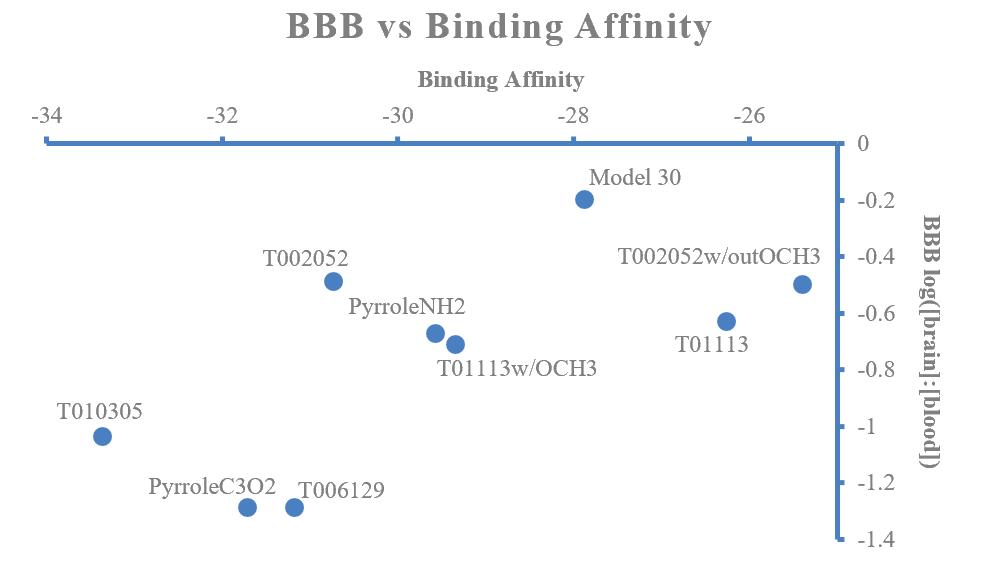
Figure 7. Blood brain barrier permeability compared to the computational binding affinities for Model 30 and candidate molecules. The upper left data points are most ideal in each respect.

Generally, candidates with better predicted inhibition had worse predicted permeability and vice versa. This made choosing compounds to synthesize more difficult. Model 30 had the most effective predicted BBB permeability (Fig. 7), but other molecules had preferable computational binding affinities. Considering that no compound stands out for excellent scores in both variables and that a goal of this particular research project is to more effectively inhibit GSK-3β particularly, the candidates with more promising binding affinity scores were selected for possible synthesis. These were molecules T0103050, PyrroleC3 0 2, T006129, and T002052. Attempting to use the reaction mechanism previously proposed and taking the availability of laboratory materials into consideration, candidate molecule T006129 was then chosen to be synthesized.

3.2 – Synthesis Analysis

The FTIR analysis of the product shows promising results for the synthesis of molecule T006129 (Fig. 8). With a yield of approximately 10%, product T006129 was concluded to have been produced.

Figure 8. FTIR data comparing the components of the T006129 product to the aldehyde reactant.

Prominent absorption lines of the reactant, including the nitrogen on the indole and the carboxylic acid group, were preserved in the product (Fig. 8). The aldehyde peaks, on the other hand, were absent in the product, confirming that the appropriate reaction did occur.

3.3 – Assay Analysis

When the GSK-3β inhibition assay was performed, product T006129 was experimentally determined to affect the performance of the GSK-3β protein. The molecule had inhibitory results when added to the reaction solution (Fig. 9). As the experiment was not able to be repeated in the limited time frame, a true IC50 score for T006129 could not be determined. Even so, initial results show that inhibitor T006129 had a 53% inhibition at a 0.98μL concentration, which is comparable to Model 30’s IC50 score of 0.89 ±0.21μL. The promising GSK-3β inhibition results of T006129 point to inhibition of hyperphosphorylation of tau. At the same time, the molecule maintains its structural features to attack early tau aggregation, suggesting that T006129 may be effective in inhibiting future stages of tau aggregation. These results support that this research approach may yield new and even more effective compounds. By refining the T006129 inhibitor’s IC50 score with more GSK-3β assay trials and testing the other promising inhibitor candidates defined in this study, the GSK-3β inhibition results may be more accurately compared. This additional research would pave the way to testing the impact of the early multitargeted approach on later stages of tau aggregation.

Figure 9. GSK-3β assay fluorescence results for com-

pound T006129 are shown above. The % inhibition was found by dividing the amount of ATP used by the enzyme with the inhibitor present by the amount of ATP used without the inhibitor present.

4. Conclusion

The multitargeted approach to treating Alzheimer’s disease with the tau hypothesis has yet to be further tested. While multitargeted molecules have been proposed, focusing on specialized binding properties may increase drug effectiveness and decrease undesirable side effects. The Model 30-derived candidate molecules outlined in this paper were computationally predicted to have more interaction with the GSK-3β protein than the baseline Model 30 molecule based on their computed binding affinities. One

such novel molecule was successfully synthesized. The assay suggests that this inhibitor was comparable to Model 30, with a 53% inhibition at a 0.98μL concentration compared to a 50% inhibition at a 0.89 ±0.21μL concentration respectively. Further investigation is required to refine the measurement of this IC50 score and determine the early aggregation inhibition as modeled by the AcPHF6 peptide.

A proper IC50 score of inhibitor T006129 could not be determined in the limited time frame. Even so, the comparable results suggest that the performance of T006129 and the other inhibitors should continue to be explored. Among the other candidate compounds explored, compounds T0103050 and T00252 computationally outperformed T006129 when taking blood brain barrier permeability into consideration with binding affinity.

Future studies should refine the IC50 estimate of T006129 with multiple replicates of assay data. The other candidate inhibitors should also be synthesized and tested for their performance against GSK-3β. Additionally, it would be wise to take factors like the AcPHF6 inhibition and blood brain barrier permeability into consideration. These inhibitors are ultimately meant to be multitargeted drugs. While the focus in this study was to improve the GSK-3β inhibition specifically, the inhibition of early tau aggregation and the dosage efficiency of the compound must be considered in future studies. The results of this study suggest that a multitargeted inhibitor with improved GSK-3β inhibition may be created, but a considerable amount of research is imperative before a treatment for Alzheimer’s disease can ultimately be proposed.

5. Acknowledgements

I would like to acknowledge Dr. Timothy Anglin, Dr. Michael Bruno, Dr. Kat Cooper, Dr. Darrell Spells, Mr. Bob Gotwals, the NCSSM Foundation, the NCSSM Science Department, the Summer Research and Innovation Program, Dr. Sarah Shoemaker, and my Research in Chemistry Peers for making this research possible.

6. Supplementary Materials

[1] Alzheimer’s Association. (2018). 2018 Alzheimer’s Disease Facts and Figures, Alzheimers & Dementia, 14(3), 367–429. doi: 10.1016/j.jalz.2018.02.001

[2] Myths. (n.d.). Retrieved from http://www.alz.org/ alzheimers-dementia/what-is-alzheimers/myths PDB ID: 1Q4L

[3] Kuret, J., et al. (2005). Pathways of tau fibrillization. Biochimica Et Biophysica Acta (BBA) - Molecular Basis of Disease, 1739(2-3), 167–178. doi: 10.1016/j.bbadis.2004.06.016

[4] Gandini, A., et al. (2018). Tau-Centric Multitarget Approach for Alzheimer’s Disease: Development of First-inClass Dual Glycogen Synthase Kinase 3β and Tau-Aggregation Inhibitors. Journal of Medicinal Chemistry, 61(17), 7640–7656. doi: 10.1021/acs.jmedchem.8b00610

[5] Bertrand, J., et al. (2003). Structural Characterization of the GSK-3β Active Site Using Selective and Non-selective ATP-mimetic Inhibitors. Journal of Molecular Biology, 333(2), 393–407. doi: 10.1016/j.jmb.2003.08.031

6.1 StarDrop Data

Compound

Oral CNS Scoring Profile Score Lipinski Rule of Five Score BBB log([brain]:[blood])

T002052 T006129 T010305 Pyrrole

C3 0 2 Pyrrole NH 2 T01113w/ OCH3 Model 30

0.1482 0.1183 0.1899 0.1219 0.1478 0.2131 0.2373

1 1 1 1 1 1 1

-0.4836 -1.284 -1.032 -1.284 -0.6675 -0.7091 -0.1947

A TELEMETRIC GAIT ANALYSIS INSOLE AND MOBILE APP TO TRACK POSTOPERATIVE FRACTURE REHABILITATION

Saathvik A. Boompelli

Abstract

Accurate and objective monitoring of a fracture’s healing process is essential to both patient quality of care and determination of the chances of nonunion and postoperative intervention. In recent years, due to industrialization, injury rates in developing countries, notably road traffic injuries (RTIs), have drastically increased. Ill-equipped countries such as Kenya may have only 60 orthopedic surgeons for a population of 36.9 million, with no rigorous rehabilitation protocol or quality post-operative care. This work focuses on the development of a telemetric gait analysis insole that works in conjunction with a mobile application. This technique automates the tedious and resource-intensive process of tracking postoperative fracture rehabilitation. This is done through analyzing patient ground reaction forces (GRFs), which have been found to correlate well with weight-bearing ability, fracture healing, and delayed union. Four force-sensitive resistors (FSRs) that function through polymer thick film technology are placed in the insole under the primary areas for force measurement. An Arduino microcontroller compiles the data and sends it to a Python program via a Bluetooth module. The Python program performs peak analysis to determine the average peak Vertical Ground Reaction Force (VGFR) of the strides. This value is sent to a cloud database that subsequently sends the data to a mobile application made accessible to a healthcare professional, who can send back weight-bearing recommendations based on the data. Features include access to the cloud database, a graph of weekly values, emailing functionality, and an ability to begin a trial through a smartphone. This approach addresses a commonly overlooked lapse in the healthcare system of many countries and provides an objective method to track fracture healing.

1. Introduction

1.1 – Motivation 1.1.1 – Lower Extremity Injury Prevalence

The economic boom occurring in developing countries comes at the cost of new and challenging problems, including the rapid increase of Road Traffic Injuries (RTIs) with the urbanization of rural areas. There is often a lack of legislation regulating the education of the local population on how to navigate the new infrastructure being constructed in their areas. This results in a higher prevalence of fractures and lower-extremity injuries in developing countries (Fig. 1), accounting for more than 1.27 million deaths per year, and more deaths than HIV/AIDS, tuberculosis, and malaria combined. However, the number of RTI injuries is more jarring, with 20-50 injured due to RTIs for every RTI related death[1]. These 60 million injured patients expected in the next ten years place a significant burden on local, unequipped medical facilities. Regional economies are also significantly impacted, with much of the local productivity reliant on human labor.

1.1.2 – Rural-Medical Practitioners and Under-Qualification

This problem of exorbitant amounts of injuries is compounded by the lack of qualified specialists and an excessive number of under-qualified physicians referred to as Rural Medical Practitioners (RMPs) who have no formal education. These RMPs tend to over prescribe painkillers in place of legitimate procedures, taking advantage of their uneducated clientele. Due to the inaccessibility of expensive equipment such as X-ray imaging devices, RMPs use subjective and often inaccurate methods to track the rehabilitation of patients with lower-extremity fractures. This research aims to connect underserved communities with more educated specialists, who are often located in larger metropolitan areas.

Figure 1. Graph depicting concentrations of Road Traffic Deaths across the globe [15]

1.1.3 – Delayed-Union and Non-Union

Approximately 5% to 10% of fractures worldwide proceed to nonunion [4], which is the improper bonding of a

fracture (Fig. 2). This leads to permanent disabilities and a significantly higher need for healthcare resources, which often can not be provided. Classically, the reasons for delayed-union and non-union are complications including inadequate reduction, loss of blood supply, and infection, all of which are extremely prevalent in developing areas [6]. A well designed post-operative rehabilitation protocol can be implemented to identify any stagnations in the healing process. However, physicians in rural areas often cannot provide quality postoperative care, leaving their patients without outpatient facilities after surgery.

Figure 2. X-Ray of a Humeral Nonunion [16]

1.1.4 – Benefits of Early Partial Weight Bearing

Early weight bearing is often absent from many rural rehabilitation protocols, with “just rest” being prescribed, as that is mistakenly seen as the best way to heal a fracture. However, early partial weight-bearing has been found to improve fracture healing, maintain bone stock and density, and keep the fracture and implants aligned early in the recovery process [5].

1.2 – Background 1.2.1 – Telemetric Medicine

Telemetric medicine is a budding subfield of biomedical engineering that allows for patient-doctor communication from thousands of miles away. This has massive potential in addressing the problems faced by underserved communities, including a lack of qualified specialists, by giving them access to these specialists. Currently telemetric medicine has been limited to first world countries, where elderly and disabled patients who are not capable of traveling to a hospital can be provided with quality care from the comfort of their home. However, current trends have shown rapid increases in the number of smartphones available to rural populations in developing countries due to a decline in phone price. This has allowed for fast data transmission to these areas. For example, vaccine reminders and natural disaster alerts have become commonplace. This research takes advantage of this framework by allowing for direct patient to doctor communication over long distances.

1.2.2 – Weight-Bearing Ability

Weight-bearing ability of the afflicted limb has been shown to greatly correlate with radiological evidence of fracture union and overall healing (Fig. 3) [4]. Accord- ing to study by S. Morshed, 84% of patients indicated that weight bearing ability was the most important clinical cri- teria for diagnosis of delayed union and non-union. De- spite weight-bearing ability being the most critical factor in the diagnosis of non-union, it is not often used due to the subjectivity of clinical observation and patient feed- back being very unreliable and incomparable over the long term. This research presents an objective method to track gait parameters, such as weight bearing ability, and allows for repeatability- crucial in the tracking of a patient’s reha- bilitation protocol.

Figure 3. Graph depicting relationship between weight bearing and fracture healing [17]

1.2.3 – Review of Insole-Based Gait Analytics Systems Currently a majority of gait analysis is performed in two specific methods: in a laboratory with force plates and 3-D motion tracking or in a doctor’s office with a clinician making visual observations. The first method is extremely expensive and provides highly specialized and unnecessary data points while the second method is very subjective and is often not repeatable over several trials and patient visits. The benefits of insole-based gait analytics have been identified as an accurate and cheap alternative to laborato-

ry and clinician-based gait analysis. Gait analysis systems measure a range of data types including foot angle, stride distance, step distance, step count, cadence, and speed . To measure the extremely different statistics that fall under the gait analysis the insoles use different sensor types for each statistic. Accelerometers are used for stride length and velocity, gyroscopes are used for orientation, flex-sensors are used for plantar and dorsi-flexion, electric field sensors for height above the floor, and finally force-sensitive resistors are used for force parameters which is the focus of this work [2].

1.2.4 – Ground Reaction Force and Biomechanics

The method utilized to measure weight bearing ability is the temporospatial gait parameter known as vertical ground reaction force (VGRF). In biomechanics, it is defined as the force exerted by the ground on the body, when in contact with the ground. Research has also suggested that ground reaction forces correlate well with callus mineralization and weight-bearing ability [3]. An increase in ground reaction force indicates increased healing for the patient. While weight-bearing is subjective, ground reaction force measurements give healthcare providers a singular statistic that can be stored and automatically processed by computers in a setting where human involvement is scarce and valuable. The VGRF graph (Fig. 4) displays the active loading peak, the point of greatest force in the gait cycle, which is the target statistic our insole aims to measure.

Figure 4. Vertical Ground Reaction Force graph over a single stride [18]

2. – Materials and Insole Design

2.1 – Insole Design Criteria

The insole was chosen as the primary data acquisition device due to the low relative cost in comparison to force plates. Force plates are traditionally used in gait analysis but are not viable as even a slight increase in cost can exponentially decrease the number of viable users. The insole was also designed to be less than 300 grams, as any heavier weight has been found to greatly alter gait parameters, resulting in inaccurate data [2]. Small, individual sensors were used in place of larger sensors, minimizing hysteresis and inaccuracy in measurements across multiple trials.

2.2 – Force-Sensitive Resistors and Placement

The insole uses 4 force-sensitive resistors (FSRs) that utilize polymer-thick film technology and provide a resistance differential based on the force exerted. Polymer-thick film sensors are constructed by the deposition of several dielectric layers via a screen-printing process, making them extremely cheap and lightweight compared to capacitive sensors. To maximize cost efficiency, 4 locations on the sole of the foot, which were identified via a pedobarograph (Fig. 5) to have the greatest concentration of force, are where the FSRs would be placed. The locations on the sole of the foot determined to have the greatest concentrations of force were under the big toe, metatarsal head I, metatarsal head V, and the heel [11].

Figure 5. Pedobarograph representing areas of highest force concentrations [19]

2.3 – Hardware Structure and Data Pathway

The data from the FSRs are then sent to an ankle-mounted Arduino Nano microcontroller attached via a Velcro strap. The Arduino microcontroller compiles the data received and uses a Bluetooth module to send the data via Bluetooth low energy signals (Fig. 6). In gait analysis, wireless technology is heavily utilized and beneficial as wired technology greatly affects the target gait parameters, resulting in non-representative data. The data are then received by the data analytics software, which is written in the Python programming language.

Figure 6. Insole hardware wiring including an Arduino Nano and HC-O6 Bluetooth Module

3. Data Analysis and Software

3.1 – Python Code and Peak Analysis

The Python program performs time-series peak analysis to acquire the active loading peak of the ground reaction force. Table 1 is an example of a raw dataset (in Newtons) that requires peak analysis. Each data point in Table 1 is taken every 30 milliseconds from the insole and is stored in the table. Figure 7 is a plot of the data in Table 1 and depicts how peak analysis functions. The red point in each step represents the active loading peak or the max VGRF for that step. An algorithm included within the code performs this process by defining a step as an array of non-zero digits separated by zeroes, where the largest value in that array is extracted and tagged as the VGRF of that individual step. The non-zero digits are the instances when the foot is in contact with the ground, while the zero digits are when the foot is in the air, providing no data to the force sensors. To provide robust and accurate data, the program is designed to average the VGRF value over multiple strides (N>6) during the trial. Six strides were chosen as the minimum number of steps needed to provide representative gait analysis data including ground reaction force [7].

3.2 – Google Sheets API

The average VGRF value is then printed to a Google Sheets API, allowing it to be accessed from any device. The Google Sheets API provides the healthcare provider with the week number relative to the beginning of the rehabil-

Table 1. Consecutive VGRF Values (Newtons) Ac-

quired from Insole (Left→Right and Top→Bottom) 0 0 0 0 203.2 364.8 389.6 406.4 429.2 403.2 324.8 194.4 0 0 0 0 0 0 0 0 183.2 348.8 367.2 373.6 388.4 364.8 0 0 0 0 0 0 208.8 336.0 365.6 372.8 393.6 404 212.8 0 0 0 0 0

Figure 7. Peak Analysis Visualization

itation protocol, VGRF values, a visual representation via a graph that is updated after every entry from the patient, and an automatic risk assessment. As this work aims to address the lack of qualified specialists, the API automates the tedious aspect of screening at-risk patients during rehabilitation. To achieve this, the API tags any patients with a stagnation or reversal of VGRF as high risk, and tags patients with increases in VGRF as low risk. Using this novel approach, the healthcare provider can address patients with a high risk of delayed or nonunion quickly and accurately.

3.3 – Smartphone Application

To provide patient-centered care, a mobile app that provides patients with data and communication tools for proper management of their injury was developed (Fig. 8) through the MIT App Inventor program. The application includes access to the cloud database, a graph of weekly values, and emailing functionality. The app also includes Bluetooth pairing capability which allows the patient to begin a trial through their smartphone. The design is focused on simplicity of use. Upon initialization of the app, the user is shown a welcome screen in which they can visit their history or begin a test. Patient history includes a table

and graph of weekly data to aid patients in visualization of the healing progress of their fracture. Testing is done over individual IP servers in order to protect privacy and connect with the API database.

Figure 8. Mobile Application Initialization Pathway

4. Results and Discussion

4.1 – Hysteresis and Quality Analysis

FSRs are rarely used in biomedical devices, as consistency and accuracy are one of the most important criteria for success, but FSRs have classically been more suscep tible to inaccuracies. An experiment was designed to test the quality of the insole, the extent of hysteresis and the inaccuracy of the sensor over time.

Figure 9. Hysteresis or inaccuracy overtime: optimized vs unoptimized sensor

Hysteresis or deviation is the inaccuracy of a sensor’s indicated values from actual values which occurs in all sensors and is accounted for. Figure 9 plots sensor hysteresis against hours of use under the stress from weight that simulates human locomotion. The control was a single unoptimized FSR, and it was compared to the insole designed with FSRs optimized by placement, size, and resistance. The graph below shows clear reductions in the amount of hysteresis for the optimized and designed insole. A 2-Sample T-Test for the final hysteresis values was performed with 30 trials, resulting in a significance value of a=.05. The test results in a p-value of 0.021 indicating statistical significance.

5. Conclusion and Future Work

5.1 – Conclusion and Real-World Application

This work addresses a commonly overlooked lapse in the healthcare system of a significant portion of the world’s population. The addressed issue of increased road traffic injuries will continue to exponentially grow in coming years. Novel solutions to the proper healthcare and rehabilitation of these injuries will be required to maintain a high quality of life for those afflicted. The hardware utilized is optimized for the specific use-case of a rural and low-income setting in conjunction with a software application designed to utilize the overdeveloped sector of communications technology in developing countries with many rural villagers owning smartphones.

5.2 – Future Work 5.2.1 – Machine Learning

Machine learning is another budding field of technology that is uprooting the medical sector by automating tasks that could previously only be performed by a trained physician. However, a drawback of machine learning and artificial neural networks is the vast amount of data needed to train and create an accurate model [14]. The data that are collected in the field from this work could contribute to gait analysis databases and allow for even more automation in this field, thereby improving the quality of life of underserved communities in developing countries.

5.2.2 – Other gait disorders

Research has shown that other common disorders such as Parkinson’s Disease and Cerebral Palsy have clear lower-extremity gait related symptoms [12][13]. As the modern hospital moves more towards the patient’s home, telemetric medicine will become heavily utilized with medical devices such as the one presented in this work.

6. Acknowledgments

I would like to express my gratitude towards Dr. Sambit Bhattacharya of Fayetteville State University for guiding me in this project. His input allowed me to find solutions in ways I never would have thought to.

7. References

[1] Mathew, G., & Hanson, B. P. (2009). Global burden of trauma: Need for effective fracture therapies. Indian jour- nal of orthopaedics, 43(2), 111.

[2] Bamberg, S. J. M., Benbasat, A. Y., Scarborough, D. M., Krebs, D. E., & Paradiso, J. A. (2008). Gait analysis using a shoe-integrated wireless sensor system. IEEE transactions on information technology in biomedicine, 12(4), 413423.

[3] Seebeck, P., Thompson, M. S., Parwani, A., Taylor, W. R., Schell, H., & Duda, G. N. (2005). Gait evaluation: a tool to monitor bone healing?. Clinical Biomechanics, 20(9), 883-891.

[4] Morshed, S. (2014). Current options for determining fracture union. Advances in medicine, 2014

[5] Dorson, Jill R. "Biofeedback aids in resolving the paradox of weight-bearing." (2018).

[6] Nunamaker, D. M., Rhinelander, F. W., & Heppenstall, R. B. (1985). Delayed union, nonunion, and malunion. Textbook of Small Animal Orthopaedics, 38.

[7] Falconer, J., & Hayes, P. W. (1991). A simple method to measure gait for use in arthritis clinical research. Arthritis & Rheumatism: Official Journal of the American College of Rheumatology, 4(1), 52-57.

[8] Rao, U. P., & Rao, N. S. S. (2017). The rural medical practitioner of India. Evol Med Dent Sci, 6.

[9] Naeem, Z. (2010). Road traffic injuries–changing trend?. International journal of health sciences, 4(2)

[10] Bachani, A., Peden, M. M., Gururaj, G., Norton, R., & Hyder, A. A. (2017). Road traffic injuries.

[11] Razak, A., Hadi, A., Zayegh, A., Begg, R. K., & Wahab, Y. (2012). Foot plantar pressure measurement system: A review. Sensors, 12(7), 9884-9912

[12] Zhou, J., Butler, E. E., & Rose, J. (2017). Neurologic correlates of gait abnormalities in cerebral palsy: implications for treatment. Frontiers in human neuroscience, 11, 103

[13] Hausdorff, J. M. (2009). Gait dynamics in Parkinson’s disease: common and distinct behavior among stride length, gait variability, and fractal-like scaling. Chaos: An Interdisciplinary Journal of Nonlinear Science, 19(2), 026113

[14] Gal, Y., Islam, R., & Ghahramani, Z. (2017). Deep bayesian active learning with image data. In Proceedings of the 34th International Conference on Machine Learning-Volume 70 (pp. 1183-1192). JMLR. org. [15] Naboureh, A., Feizizadeh, B., Naboureh, A., Bian, J., Blaschke, T., Ghorbanzadeh, O., & Moharrami, M. (2019). Traffic accident spatial simulation modeling for planning of road emergency services. ISPRS International Journal of Geo-Information, 8(9), 371.

[16] Edginton, J., & Taylor, B. (2019). Humeral Shaft Nonunion. OrthoBullets

[17] Joslin, C. C., Eastaugh-Waring, S. J., Hardy, J. R. W., & Cunningham, J. L. (2008). Weight bearing after tibial fracture as a guide to healing. Clinical biomechanics, 23(3), 329-333.

[18] Larson, P.(2011). Vertical Impact Loading Rate in Running: Linkages to Running Injury Risk.

[19] Tekscan, F-Scan System. https://www.tekscan.com/ products-solutions/systems/f-scan-system.

DIFFERENCES IN RELIABILITY AND PREDICTABILITY OF HARVESTED ENERGY FROM BATTERY-LESS INTERMITTENTLY POWERED SYSTEMS

Nithya Sampath

Abstract

Solar and radio frequency (RF) harvesters serve as viable alternative energy sources for battery-powered devices in which the battery is not easily accessible. However, energy harvesters do not consistently produce enough energy to sustain an energy consumer; thus, both the energy availability and execution of the consumer process are intermittent. By simulating intermittent systems with large-scale energy demands using specifically designed circuit models, parameters including harvested voltage, voltage across the capacitor, and voltage across the consumer were determined. The probability of energy availability was then computed based on the number of energy events that had previously occurred for both harvested solar and radio frequency. A metric designated as the η-factor was computed from the probability plots for the solar and radio frequency data to quantify the reliability of each power source. The η-factor for harvested solar energy was significantly higher than that of harvested radio frequency energy, indicating that harvested solar energy is more consistently available than harvested radio frequency energy. Finally, the effects of various obstacles between the radio frequency transmitter and receiver on the output voltage were determined. Increasing the distance between the transmitter and receiver, as well as placing people and metal between the two, resulted in a significant drop in energy availability as compared to foam and wood obstacles. Quantifying the reliability of different harvested sources would help in identifying the most practical and efficient forms of renewable energy. Determining which obstacles cause the most obstruction to a signal can aid in optimizing the strategic placement of harvesters for maximum energy efficiency.

1. Introduction

Battery-powered devices such as pacemakers and neurostimulators are not suitable in many systems due to their inaccessible placement and frequent need for battery replacement. Harvested energy from solar, radio frequency, and heat sources is an attractive alternative to batteries in such systems; however, energy availability from these sources is not consistent and is therefore characterized as intermittent. There are two components to these intermittently powered systems: the energy harvester and the energy consumer. The energy consumer utilizes the energy captured by the energy harvester. For the energy consumer to remain functional, a certain power threshold must be met. There is often a discrepancy between the amount of energy required to power the consumer and the amount of energy supplied to the system by the energy harvester, causing the device to cyclically turn on and off as shown in Figure 1. This sporadic energy harvesting pattern leads to an interrupted, or intermittent, execution of the energy consumer [1]. Most renewable energy sources, including solar and wind power plants, have an intermittent power output [2].

An energy event is defined as the generation of a significant voltage in a given time interval. In this study, a minimum voltage of 2.8V during a period of 5 minutes was considered significant. Indicating that N energy events have occurred signifies that 5N minutes have passed since the energy consumer last shut off. The time designated for an energy event in this investigation was selected to test the burstiness of energy and accurately determine when the probability of a future energy event reaches 0. A capacitor was included in the circuit to store and release energy slowly into the consumer. Without the capacitor, energy flowing directly from the harvester to the consumer would instantly terminate the execution of the consumer software in the absence of an energy event [3].

Figure 1. Graph of voltage vs. time for an energy consuming device. The device turns on when it reaches a threshold voltage, approximately 2 Volts, and begins to consume energy at a rate greater than the rate at which harvested energy is supplied to the circuit. When the voltage supplied to the energy consuming device drops, the device shuts off and the voltage is allowed to increase again from the harvested power supply. This cycle repeats.

The objective of this study is to model an energy harvesting system on a small scale using solar harvester and radio frequency harvester units. This model will be used to analyze the burstiness of energy by computing the likelihood of power availability, given that N consecutive energy events have occurred. It is hypothesized that all harvested energy will be available in short bursts, consistent over small periods of time. The reliability of various harvested sources in terms of their power availability will also be determined by computing the η-factor. The η-factor is a metric that compares the experimental energy harvesters to a random energy harvester, in which energy events are independent. This is not the case for real energy harvesters, in which energy events are dependent upon each other. It is predicted that the η-factor of solar energy will be higher than that of radio frequency energy, both of which will be less reliable than wall power, which has a η-factor of 1.0. Lastly, the effect of various obstacles and distances between an RF transmitter and receiver will be determined. It is expected that obstacles with a higher density, such as people, will allow for less energy to be harvested than obstacles such as foam or wood. Obstacles were considered only for harvested RF energy, as solar energy is traditionally harvested without obstruction. This research currently has great relevance as the world begins to look towards renewable energy sources to replace fossil fuels. Investigating the patterns of energy availability and consumption allows for precise prediction of energy patterns and optimization of execution process scheduling.

2. Materials and Methods

The setup for both the solar and the radio frequency experiments involved two main circuits as shown in Figure 2. The first, designated as the harvester circuit, captured energy either from the sun or from the transmitted RF signal and converted it into electrical energy. There were 4 main components to this circuit: the solar or radio frequency harvester unit, the capacitor, the LTC (Load Tap Changer), and the consumer. In this experiment, the load was an MSP-430 device that was constantly running an energy-consuming software and required 2.8 Volts to turn on. The purpose of the LTC in the circuit was to ensure that given a certain amount of energy input, the amount of voltage output would be 3.3 Volts. This amplified input voltage pronounces the absence of sufficient energy. The voltage was recorded across the energy consumer and energy harvester, which captured energy from the sun or radio frequency transmitter. The weather conditions during the experiment are important to consider when dealing with solar data. A light sensor was used to record the full-spectrum, infrared, and visible light levels. The device also retrieved real-time weather data from Weather. com, including the temperature and UV index. The experiment was conducted under consistent weather conditions, sunny and minimal cloud coverage, and the harvester was placed directly across from a window facing west. The system tended to reach peak energy in the afternoon, when the most sunlight was available.

Figure 2. Diagram of circuit setups for solar and radio frequency harvesting experiments. Output voltages from each component in the harvester circuit — the harvester unit, the capacitor, the LTC, and the load — were connected to the Arduino and recorded.

For the radio frequency experiment, an infrared sensor was also used to record the presence and absence of people; a person walking in front of the sensor and blocking the signal was considered as an absence of an energy event. A secondary logger circuit was constructed to record voltages at each point in the harvester circuit. It consisted of a Raspberry Pi 3 and an Arduino Uno, powered from the wall. Arduino and Python programs were used to record and analyze the voltage data, calculate η-factors, and construct plots of energy availability.

The obstacle experiment with a radio frequency harvester involved a similar setup, except for an infrared sensor. Python and Arduino programs were used to record the voltages at various points in the circuit. Data were collected over a span of 2 minutes each for four different obstacles–metal, wood, person, and foam–over three different distances – 1 meter, 2 meters, and 3 meters. The voltages were recorded from the D out pin on the MSP-430, which is directly related to the amount of radio frequency input received. The absence of an obstacle between the transmitter and the receiver served as a control to which the other voltage values were compared. The approximate densities and thicknesses of the obstacles used are listed in Table 1. The density of a human was approximated to be 1.01 grams per cubic centimeter [4].

3. Results

This study aimed to test the burstiness properties of harvested energy by analyzing the probability of energy availability. The idea that energy was available in short

Table 1. Approximate thicknesses and densities of obstacles used in experiment. The thicknesses were measured and densities were calculated using measurements of mass and volume. The thickness measurement for a human is very approximate as it is harder to measure with precision.

Approximate Thickness and Density of Obstacles Thickness (cm) Density (g/cm3)

Human 25 1.01 Metal Whiteboard 2.0 0.85 Wood 2.0 0.70 Foam 0.3 0.13

bursts was suggested by earlier data collected in the lab; however, the data collection did not occur for long enough to prove conclusions supporting that idea. To determine whether the energy-consuming device was turned on and how much energy was being supplied to the circuit, voltage data was recorded at various locations in the circuit. In Figure 3 (solar) and Figure 4 (radio frequency), the horizontal axes contain both positive and negative values for the number of previous energy events. Negative numbers of energy events correspond to a continuous absence of energy events. These graphs support the hypothesis of the burstiness of harvested energy since the probability does not oscillate as the number of energy events increase.

Figure 3. Probability plot for harvested solar energy. This plot displays energy occurring in short bursts.

The mean η-factor is 0.8595 (n = 6). The data collection

for this experiment spanned three days.

Figure 3 also depicts that the correlation between the probability and the number of energy events decreases near N = 70. This is consistent with the designated definition of an energy event, as 70 energy events lasting 5 minutes each would cumulate to 5.83 hours. This is the approximate time for which sufficient sunlight was facing the energy consumer in the experiment location. This feature is not represented in Figure 4 as the amount of harvested radio frequency energy was not dependent upon the time of day.

Figure 4. Probability plot for harvested radio frequency energy. This plot displays energy occurring

in short bursts. The mean η-factor is 0.3657 (n = 6).

The data collection for this experiment spanned two weeks.

The reliability of various harvested sources based on the η-factor was compared. The findings reinforce the hypothesis of a given harvested energy source being more reliable than another due to the variance in reliability patterns. The mean η-factor for harvested solar power was 0.8595 and the mean -factor for harvested radio frequency power was 0.3657. The standard deviation of the solar data was 0.0018 and the standard deviation of the radio frequency data was 0.0762. A student’s t-test was performed over the 6 trials for each of the solar and radio frequency experiments. The t-test yielded a two-tailed p-value of less than 0.0001, indicating a statistically significant difference between the η-factors for harvested solar and harvested radio frequency energy. The η-factors for both harvested solar and harvested radio frequency energy fall below the ideal standard of 1.0, the η-factor for wall and battery power. This can be observed in Figure 5, where the probability of energy availability, given that any number of energy events have occurred, is 1.0 [5]. The higher η-factor for solar power suggests that harvested solar energy is more reliable than harvested radio frequency.

Finally, various obstacles and distances separated a radio frequency transmitter and receiver to determine how they would affect the amount of harvested energy. Varying obstacles are likely to have varied effects on the amount of energy able to be harvested, due to the density and thickness of the object. The results shown in Figure 6 indicate that metal and people had a more pronounced effect on the ability of the receiver to harvest energy from the transmitter as compared to wood and foam. Foam had a slightly higher voltage input value than the absence of an obstacle at 1 meter, but this difference is too small to be significant and was likely caused by random variation. Additionally,

as distance increases, the received signal input decreases for all obstacles. Over larger distances, fewer signals can be received and converted into electrical energy.

Figure 5. Theoretical probability plot for wall pow-

er. Wall power has a η-factor of 1.0 since it is not in-

termittent.

Figure 6. Graph depicting D for various obstacles out and distances in the RF obstacle experiment. The Dout value is correlated with the radio frequency input, so higher D values correspond to higher radio freout quency input.

4. Discussion

The major objectives for this investigation included investigating the burstiness of energy, comparing the reliability of harvested solar and harvested radio frequency energy, and exploring the effects of various obstacles and distances on the amount of harvested radio frequency energy. Graphs of the probability of energy availability given that a certain number of energy events had occurred were constructed and analyzed from which η-factors were calculated (Fig. 3 and 4). The average Dout values for different obstacles and distances were also plotted against a control group, comparing which obstacles had the greatest effect on D out values (Fig. 6).

Figures 3 and 4 indicate the burstiness of both harvested solar and radio frequency energy. The probability of an energy event occurring becomes relatively high, after many have already occurred. This correlation does not continue in the case of harvested solar energy. Increasing the time interval t, which defines an energy event, could have had an influence on this data. A larger value of t may represent sections of the graph after the correlation ends for solar energy, causing probabilities in the middle to appear closer to 1 than they truly are. Selecting a smaller value of t may not show where the correlation ends, suggesting that the correlation does not in fact end. In Figure 4, there is a spike in probability at approximately N=-1. This indicates that if there was no energy event in the previous time interval, then the probability of a future energy event is extremely high. This suggests that when a person walks in front of the sensor, they cause the absence of a single energy event, but they are not likely to cause the absence of a second energy event. In other words, most people walk by the sensor rather than standing in front of it. Inaccuracies in the infrared sensor, indicating if a person was blocking the signal, may have also influenced the results. Finally, the Arduino could only record voltages to 2 decimal places, limiting the precision of the data analysis. This analysis of the burstiness of energy will allow for the optimization of scheduling execution processes.

The calculations of the η-factor and the results of the student’s t-test suggest that harvested solar power is more reliable than harvested radio frequency power, supporting the original hypothesis. The increased standard deviation for the radio frequency-factor could be attributed to the increased variance among trials in the patterns of people passing in front of a sensor over a given time, compared to the more stable pattern of light reaching a solar panel. Data collection for the harvested radio frequency energy, which lasted 2 weeks, spanned a longer period than that of solar data, which lasted 3 days. The rationale behind this was that the absence of radio frequency energy events is less frequent than the absence of solar energy events, so more data are needed to gain a holistic understanding of the radio frequency energy patterns. As in the first experiment, the reliability of the sensor and Arduino device could have also influenced the data collected. These results indicate that harvested solar energy may be a more suitable alternative to harvested radio frequency energy in terms of reliability and predictability.

The results presented in Figure 6 suggest that people and metal, more than other obstacles, obstruct the radio frequency signal from being received and converted into electrical energy. Thus, people were used to obstruct the signal in the first radio frequency experiment in order to induce the absence of an energy event. Factors that may have influenced the results include the presence of multiple objects between the transmitter and receiver, such as a foam board being held by a hand. These results are relevant to the real-world application of harvested radio frequency energy, including Wi-Fi routers and cell towers. In addition, the results indicate which obstacles are more likely to cause the absence of an energy event and can in-

form the placement of radio frequency energy harvesters.

There were limitations in some aspects of the model regarding accurately modeling large-scale solar and radio frequency energy harvesting systems. For the radio frequency experiment, the model fails to account for the real-life conditions of multiple obstacles or static obstacles, which could decrease the likelihood of energy events by allowing for less energy to be successfully harvested.

Future research may involve testing different forms of harvested energy under various weather conditions. The differences in amounts and reliability of harvested energy between different types of piezoelectric energy could be investigated, including energy harvested from mechanical stress inside a person’s shoe or energy harvested from mechanical stress on a tile. As solar cell technology advances, the reliability of different types of solar panels could also be tested.

In the search for fossil fuel replacements in this era of climate crisis, the reliability of different harvested energy sources should be considered. Harvested solar energy was found to be more reliable than harvested radio frequency energy, and this should be a factor in deciding which types of renewable energy to invest in and implement on a large scale. These harvesters, particularly radio frequency harvesters, should be placed in a way that minimizes obstruction, particularly from people and metal. In this way, energy efficiency can be maximized. Through harvesting energy from common and everyday sources like the sun and radio frequency signals, the first steps are taken towards ensuring a more sustainable and energy-efficient future.

5. Acknowledgements

Thanks to Dr. Shahriar Nirjon and Bashima Islam of the Department of Computer Science at UNC-Chapel Hill and to Dr. Sarah Shoemaker, Ms. Shoshana Segal, and Mr. Chris Thomas of the NCSSM Mentorship and Research Program for advice and assistance throughout the research process.

6. References

[1] Lucia, B., Balaji, V., Colin, A., Maeng, K., & Ruppel, E. (2017). Intermittent computing: Challenges and opportunities. In 2nd Summit on Advances in Programming Languages (SNAPL 2017). Schloss Dagstuhl-Leibniz-Zentrum fuer Informatik.

[2] Fuchs, E., & Masoum, M.A. (2015). Power Quality in Power Systems and Electrical Machines (2nd ed.). Academic Press Inc.

[3] Islam, B., Luo, Y., Lee, S., & Nirjon, S. (2019, April). On-device training from sensor data on batteryless platforms. In Proceedings of the 18th International Conference on Information Processing in Sensor Networks.

[4] Density of Human body in 285 units and reference information (2019). Retrieved November 9, 2019.

[5] Islam, B., Luo, Y., & Nirjon, S. (2019). Zygarde: Time-Sensitive On-Device Deep Intelligence on Intermittently-Powered Systems. arXiv preprint arXiv:1905.03854.

APPLYING MACHINE LEARNING TO HEART DISEASE DIAGNOSIS: CLASSIFICATION AND CORRELATION ANALYSES

Sahil Pontula

Abstract

Classification machine learning has emerged to quickly and efficiently analyze large sets of data and make predictions about potentially unknown variables. It has seen application in numerous fields, from sorting through ionosphere signals to predicting weather. Here, we report on the application of classification algorithms to heart disease diagnosis, run on a sample dataset of 303 patients. We test several models and compare their results to determine accuracy in predicting presence or absence of heart disease. Furthermore, we conduct statistical and graphical analyses to determine correlations and causations between different attributes linked to cardiovascular disease. We believe that the methods demonstrated here show promise for large-scale applications, for both more complex and comprehensive datasets and real-time data collected in a clinical setting.

1. Introduction

1.1 Heart Disease 1.1.1 Angina

Approximately 9.8 million Americans are thought to suffer from angina pectoris, or simply angina, annually, and it is suspected that 500,000 new cases emerge each year [1]. Angina is a common symptom of heart attacks (myocardial infarctions) and is the result of insufficient blood supply to the heart (cardiac) muscle, known as ischemia. In ischemia, the heart does not receive enough oxygen to pump adequately. Despite angina’s relative commonness, it can be difficult to distinguish between other causes of chest pain. The chest pain of the patients whose data we investigate here is classified as anginal or non-anginal (and the cause may be known or unknown).

Symptoms of angina include chest pain, pain in the limbs or jaw that accompanies chest pain, nausea, sweating, fatigue, and shortness of breath, though symptoms for females can be different from the conventional symptoms, and as such treatments will vary. Angina can be classified as stable or unstable. Stable angina is more common and can occur during exercise (and disappear upon resting). It occurs when the heart is required to pump much harder, is short-lasting, and is often predictable. Unstable angina is more dangerous and may indicate risk of a heart attack (it is unpredictable and longer-lasting). A third type of angina, variant or Prinzmetal’s angina, is rarer and is caused by a spasm in the coronary arteries [2].

Most often, the ischemia that causes angina is due to coronary artery disease. When coronary arteries are blocked by fatty deposits, or plaques, the condition is known as atherosclerosis. Exercise-induced angina occurs when the effects of ischemia are felt during exercise (reduced blood flow through coronary arteries cannot match the oxygen demand).

Risk factors of angina include tobacco use, diabetes, high blood pressure, high blood cholesterol levels, elderly age, sedentary lifestyle, obesity, and stress. We investigate just some of these factors in analyzing the given dataset.

1.1.2 Age

It is known that individuals of age 65 or older are more susceptible to developing heart disease, including myocardial infarctions (heart attacks) and heart failure. With older age, the heart cannot beat as quickly during exercise or stress, even though the heart rate is fairly constant. Aging commonly causes the arteries to grow stiffer, resulting in a condition known as arteriosclerosis. This, in turn, results in complications such as hypertension. Other changes in the cardiovascular system that result from aging include arrhythmias (irregular heartbeats or abnormal heart rhythms) and edema.

1.1.3 Gender

At younger ages, males are more vulnerable to heart disease than women; on average, men suffer their first attack at age 65, while women suffer their first attack at age 72 [3]. Nevertheless, heart disease is the most prevalent cause of death in both genders. Many factors may contribute to the greater vulnerability of males, including higher rates of risk factors such as smoking and the fact that hormones in younger women protect against heart disease. Additionally, the symptoms may differ between the genders; some researchers have noted that during heart attacks, women are more likely to suffer from abnormal symptoms.

Ironically, the survival rate after developing heart disease shows a trend opposite to that of acquiring it. Survival rates have been found to be lower in women, perhaps because women are less likely to obtain advice or beneficial

medications than men or because women are generally older and suffer from other health complications [3].

1.1.4 Cholesterol

Cholesterol, in normal levels, is essential for many body functions, including building new cell walls and making steroid hormones. In excess amounts, however, cholesterol tends to accumulate in arterial walls, resulting in a condition known as atherosclerosis. This disease results in narrowed arteries and blocked or slowed blood flow, causing angina or heart attacks. Note that blood-borne cholesterol is generally characterized as low-density lipoproteins (LDLs) or high-density lipoproteins (HDLs). LDLs are responsible for the atherosclerosis-causing fatty plaques. HDLs are thought to function in clearing the blood of excess cholesterol. Additionally, high levels of triglycerides, another type of fat, are suspected to correlate with occurrences of heart disease [4].

1.1.5 Electrocardiograms (ECGs)

ECGs provide a convenient way to measure the electrical activity of the heart, and hence find common application in diagnosing cardiac disorders. A representative signal of normal cardiac electrical activity is shown in Figure 1. The P wave is associated with atrial depolarization, the QRS complex is associated with ventricular depolarization and atrial repolarization, and the T wave is associated with ventricular repolarization. The measurements are recorded from a set of electrodes placed on the skin and the results are typically presented as a “12-lead ECG,” which has 12 voltage-time graphs.

Figure 1. A sample ECG signal for a normal (sinus) rhythm, showing the P wave, QRS complex, and T wave [6].

The ST segment connects the points marked S and T in Figure 1. ST depression, wherein the ST segment is unusually low relative to the baseline, is sometimes associated with heart disease. It is generally indicative of myocardial ischemia, which is primarily caused by coronary artery disease (CAD), in which blood flow is greatly reduced for much the same reason as in atherosclerosis. ST depression is also seen in patients with unstable angina. The ST segment may be depressed but also upsloping, in which case ischemia is generally not the cause. Instead, it is likely a variant of the normal sinus rhythm. Additionally, studies have shown that the ST segment slope may provide an accurate diagnosis of CAD [5].

1.2 Classification Algorithms

Here we describe the algorithms (and other related concepts) used in the classification analysis of the heart disease dataset.

1.2.1 KNN Algorithm

The KNN, or k-nearest neighbors, algorithm (Fig. 2) is part of supervised machine learning techniques (“supervised” indicates that labeled input data is being used for train- ing/testing). The algorithm assumes that data similarly classified are also close together geometrically (usually measured by the Euclidean distance).

Figure 2. The steps of the KNN classification algorithm. Note how distances are computed for the new data point between it and members of the preexisting classes before a decision is made for its classification [7].

For classification, it works by computing the distance between a data point and all other data points, selecting the k nearest neighbors thus found (where k is defined by the

user), and classifying according to the most frequently occurring label. However, this algorithm can slow significantly as the size of the dataset grows. In addition, the user must decide on the value of k. If k is too small, the dataset could be overfitted, leading to significant variance, while if k is too large, the data may be oversampled, resulting in bias.

1.2.2 Decision Tree Analysis

Decision trees function in classification and regression in machine learning. They are conventionally drawn such that their root is at the top. Conditions, or internal nodes, are places where the tree splits into branches (edges). When the branch does not split any more, we have found the decision (leaf). Decision trees allow relations and important features to be easily seen.

Decision trees are often based off of the technique of recursive binary splitting, where the split points are selected based on a cost function. This allows selection of the splits that maximize the tree’s accuracy. Sub-splits are also chosen recursively in this manner, so recursive binary splitting is also known as the greedy algorithm, as the only goal is to minimize cost. This means the root node, at the top of the tree, is the best classifier. Gini scores, G = ∑pk(1 −pk), provide a good way to quantify how good a split is by measuring how independent or mixed the two resulting groups are. An ideal split would have G = 0.

Note, however, that trees that are too long may overfit the data, and as such the number of training inputs used for splitting is often limited.

1.2.3 Support Vector Machine Analysis

This supervised learning algorithm’s objective is to find a hyperplane in n-dimensional space, where n is the number of features in the data, that classifies the data by separating the classes as much as possible. Many planes are possible to separate two given classes, but the one that maximizes the distance between data of different classes, or margin distance, is chosen.

Support vectors are data points that lie closer to the hyperplane and affect its position, directly affecting the margin distance. Note that the margin distance is optimized by a loss function known as the hinge loss function.

1.2.4 Neural Network Analysis

Typically, neural networks (NN) are the preferred method of choice for classification tasks such as this one. These structures consist of an input layer, an output layer, and a series of hidden layers in between. All layers may consist of multiple neurons (or nodes), which take in some input value, perform a computation using some algorithm, and propagate an output value to the next neuron. In the end, the output from the output layer determines the result. For classification tasks, the NN uses training data to adjust the “weight” of the algorithm/computation that the neurons use, where it can correct the values of the “weight” to match the outputs of the training data. Once trained, the NN can be used on a test set, predicting the appropriate classifications. The results can be compared with the true classifications to determine the accuracy of the model, and eventually the model can be used with real-world data.

1.2.5 Random Forest Analysis

Random forests consist of many individual decision trees working as an ensemble. Each tree outputs a class prediction, and whichever class is predicted the most by the trees is chosen as the model’s prediction. The random forest algorithm is one of the best among supervised classification techniques, because it works by integrating the predictions of many independent, uncorrelated models (trees), compensating for the individual errors of any one tree [8].

1.2.6 Naive Bayesian Analysis

This classification technique is based on Bayes’s theorem for computing conditional probabilities. It assumes independence among predictors/features in the data, and uses Bayes’s theorem to predict the probability of a given data point falling into a certain class based on the predictors.

Naive Bayes is a quick, efficient way to classify data with multiple classes. Unfortunately, it is accurate only if the assumption of independence between predictors holds. Additionally, Naive Bayes is often better with categorical variables, as it assumes numerical variables are normally distributed. Nevertheless, the fast nature of the algorithm makes it a preferred method for real-time and multi-class prediction [9].

1.2.7 Gini Index

This index measures the probability of a specific variable being wrongly classified when randomly chosen. G = 0 or G = 1 indicate that all elements are in only one class or the elements are randomly distributed across the classes, respectively. G = 0.5 indicates equal distribution of the elements in the classes.

The Gini index is defined as G = 1 − ∑(pi)2, with pi being the probability an element is classified in a specific class. In decision trees, the feature with the lowest Gini index is usually chosen as the root node [10].

1.3 Objective

In this investigation, we have two primary purposes. First, we attempt to use statistical analysis in R/RStudio, including correlograms and the Bayesian information criterion, to identify potential correlations and causations among the variables in the heart disease dataset, described in more detail below. Second, we use classification machine learning algorithms, also in R/RStudio, to predict the presence of heart disease in arbitrary patients.

The data for this work were obtained from https:// archive.ics.uci.edu/ml/datasets/heart+Disease. Data were collected from 303 patients. The original dataset consists of 75 variables, but we only consider a subset of the 14 most important variables (which were used in published experiments). The last variable is the class variable, referring to the presence or absence of heart disease. Values of 1, 2, 3, and 4 denote presence (according to a scheme used by the creators of the dataset), while a value of 0 denotes absence. The 14 variables in the dataset are as follows: 1. Age, numerical 2. Gender, categorical 3. Chest pain type, categorical 4. Resting BP (mmHg), numerical 5. Serum cholesterol concentration (mg/dl), numerical 6. Fasting blood sugar concentration (mg/dl), categor ical 7. Resting EKG results, categorical 8. Maximum heart rate (bpm), numerical 9. Presence of exercise-induced angina, categorical 10. ST segment depression due to exercise, numerical 11. Slope of peak exercise ST segment, categorical 12. Number of major vessels colored by fluoroscopy, categorical 13. Status of defect, categorical 14. Diagnosis of heart disease, categorical

3. Data Preparation and Modeling

In order to clean the data, data munging was performed in R/RStudio. The raw data were read as a CSV file directly from the URL above. The columns were then renamed to readable forms and missing data were found and corrected for. Six rows had missing data, and we chose to simply delete these from the dataset. We then reclassified the categorical variables, changing the numbers to more readable text.

4. Correlation Analysis

For preliminary analysis, pairwise histograms and correlations (scatter plots and correlation coefficients) were produced for the five numerical variables. From the histograms, it was noted that most numerical variables showed only slight skew and the only variable with considerable skew (ST segment depression) could not be easily corrected with normalization transformations. As such, the data were not transformed in any way. Furthermore, a correlogram was generated, taking the numerical variables in pairs, to visualize any correlations present.

Linear regressions were then created with ST segment depression as the dependent variable. A multiple regression model was also developed to predict ST segment depression.

To examine causality, Bayesian information criterion (BIC) values were generated between ST segment depression and each of the other variables. If the value for the association between ST segment depression and a given variable was more than 10 less than the value with no coupling, a causal relationship was possible.

Lastly, two scatterplots were generated with ST segment depression as the dependent variable and maximum heart rate as the independent variable. Points were grouped by two categorical variables, namely slope of peak exercise ST segment and type of chest pain.

5. Classification Analysis

After designating the diagnosis variable as the class variable, Gini indices were generated for all other attributes. Lower values indicated more important variables, namely those that would give greater equality in the distribution of data into classes. These variables, in turn, could be used as root nodes in decision trees. The attributes with the lowest Gini indices were plotted using jitterplots, where the dependent variable was heart disease diagnosis, to examine data clustering.

With these important variables identified, various classification algorithms were then tested. Among these were the random forest, partition, neural network, support vector machine (SVM), and Naive Bayes models. These algorithms were run on two of the “best” categorical variables (according to the Gini coefficients) and the best numerical variable, ST segment depression. k = 3 clusters were used for the neural network model, based on the jitterplots. Tables were generated to document the accuracy of the algorithms in predicting presence or absence of heart disease in the 303 patients.

Additionally, a k-nearest neighbors (KNN) algorithm was run. 70% of the dataset was designated for training, and the remaining 30% was used to test the model. A cross table of the model’s predictions and the actual diagnoses was then produced and compared with the results of the other classification algorithms.

6. Results

6.1 Correlation Analysis

The pairwise correlations and histograms for the numerical variables are shown in Figure 3. The correlogram for the numerical data are shown in Figure 4. Note from both figures that most numerical data are distributed over a range of values (i.e. more continuous than discrete). We do not see particularly strong correlations, but this does not rule out associations between the variables, as considerable scatter may be present in the data.

Linear regressions between ST segment depression and each of the other numerical variables are shown in Figure

5. Again, we see no strong correlations. At discrete values of age and resting blood pressure, we note that the data points take on a range of ST segment depressions. From the multiple regression plot shown in Figure 6, we again see considerable scatter. Indeed, when the actual ST segment depression is 0, the predicted depression adopts a wide range of values.

Figure 3. Pairwise histograms and correlations for the numerical variables. Note how the age histogram is fairly normally distributed. The histograms for resting BP and cholesterol level show right skew, the histogram for maximum HR shows left skew, and the histogram for ST depression shows significant right skew. No strong correlations appear to be present, the strongest being between age and maximum HR.

Figure 4. A correlogram for the numerical data in the heart disease dataset. The results shown confirm the findings from the pairwise plots. No strong correlation are apparent. Note that the color indicates the the direction of the correlation (positive, negative, or no correlation) and the size of the circle indicates the relative strength of the correlation. Figure 5. Four linear regressions with ST segment depression as the dependent variable. Age (years), maximum heart rate (bpm), resting blood pressure (mmHg), and blood cholesterol concentration (mg/ dl) are the independent variables.

Figure 6. A plot of the actual ST segment depression and the predicted depression using a multiple regression model with all four other numerical variables.

Conducting BIC analyses with ST segment depression as the dependent variable, it was found that half of the variables had a possible causal relationship. Among these were chest pain type, maximum heart rate, presence or absence of exercise-induced angina, slope of the peak exercise ST segment, and presence or absence of heart disease. The latter two had the lowest BIC values.

Figure 7 shows plots with ST segment depression and maximum heart rate, grouped by two categorical variables. All variables showed evidence of correlation via the regressions or BIC analyses. Grouping by slope, we see that flat and downsloping ST segments show considerable scatter, with the downsloping datapoints suggesting potential outliers at high depressions. The upsloping ST segments seem to be concentrated at low depressions. A similar trend is seen in the second graph, where asymptomatic chest pains suggest outliers. Nevertheless, none of the four categories shows distinctive patterns in the plot.

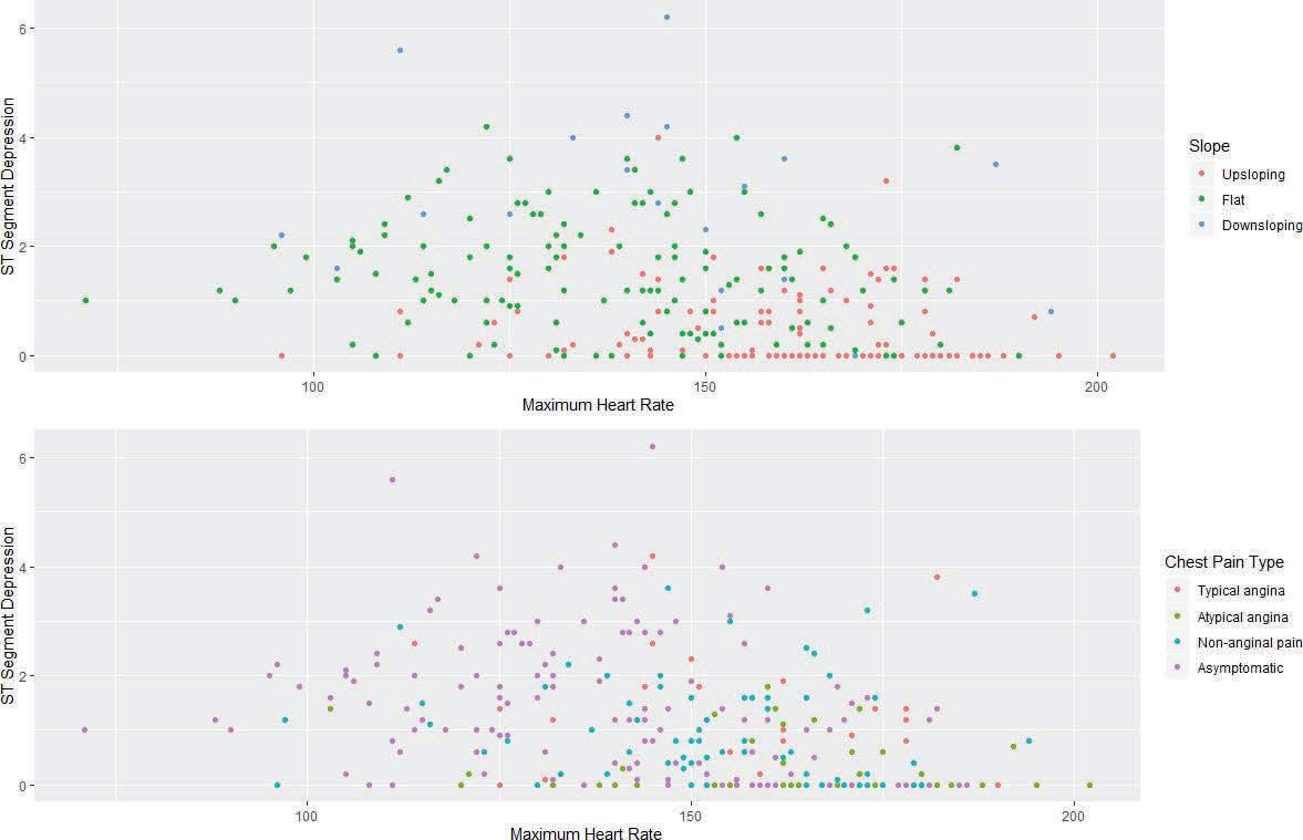
Figure 7. Two scatter plots with ST segment depression as the dependent variable. The data points are grouped by the categorical variables chest pain type and slope of ST segment during peak exercise.

6.2 Classification Analysis

By finding Gini values for each of the non-class variables, it was found that gender, fasting blood sugar concentration, and presence/absence of exercise-induced angina were most important. None of the numerical variables were major predictors of diagnosis. Nevertheless, we show jitterplots for the three aforementioned categorical variables as well as the numerical variable with the lowest Gini index in Figure 8. The three plots for categorical variables show four distinct clusters, as expected. The plot with fasting blood sugar (FBS) shows a concentration of data at low FBS values, while the plot with exercise-induced angina shows that most patients lacked both it and heart disease. In the plot with ST segment depression (the numerical variable), it is apparent that most patients presented with low ST segment depression (especially those without heart disease), with a few outliers at high depression values.

Figure 8. Four jitterplots for the variables with the lowest Gini indices. Note the distinct clustering tendency of the datapoints, indicating that most of these variables are good clustering attributes and likely important parts of any classification algorithm.

Table 1 shows the results of five of the classification algorithms. Similar accuracies among many of the algorithms can be explained given that the dataset is not too complex, so for most data points, the algorithms operate similarly and give the same predictions. The accuracy of the KNN algorithm, using all non-class variables as predictors, was 64.9% for absence and 46.3% for presence of heart disease (using the test dataset). We see that the partition model using ST segment depression as a predictor has the best accuracy for both absence and presence.

Table 1. The results of the classification algorithms, excluding KNN. The first and second numbers in each cell indicate the accuracy in predicting absence or presence of heart disease, respectively. The partition model appears to have the optimal accuracy in predicting both absence and presence, using ST segment depression as a predictor. Factors were chosen based on Gini indices and the correlation analysis.

Naive Bayes 58.1 57.7 85.6 54.0 86.9 46.7

SVM 57.5 59.9 85.6 54.0 81.9 59.1 Neural 57.5 59.9 85.6 54.0 71.3 67.9 Net Partition 57.5 59.9 85.6 54.0 91.3 68.6 Random 57.5 60.0 85.6 54.0 81.9 54.0 Forest

7. Discussion and Conclusion

In this paper, we have conducted correlation and classification analyses for a dataset containing heart disease data for 303 patients. We find that, among the numerical variables in the dataset, all pairwise correlations are weak, the strongest existing between age and maximum heart rate. These variables exhibit a weak negative correlation, which could exist for multiple reasons. For example, it has been found that aging slows the natural electrical activity of the heart’s pacemaker, the sinoatrial (SA) node [11]. The cause has not been exactly identified, but it is suspected to be due to changes in the ion channels of sinoatrial myocytes, cells in the SA node. And yet, the correlation is not at all strong. This is an indication that multiple factors contribute to maximum heart rate and similar measures of heart health, including exercise and diet. Without knowing the exact details of the patients whose data were used, we suspect that the considerable scatter in the maximum heart rateage regression is due to a variety of lifestyles. This claim is supported by the relatively wide range taken on by the histograms in Figure 3.

By creating linear regressions with ST segment depression as a dependent variable, we have found that weak positive correlations exist between it and blood cholesterol levels, age, and resting blood pressure, while a negative

correlation exists between it and maximum heart rate. We can theorize why these correlations exist, but more data would be required to confirm their statistical significance. High blood cholesterol levels are a known risk factor for atherosclerosis and CAD due to the formation of fatty plaques blocking blood vessels. Given that ST depression is an indication of these diseases, the correlation is expected. Age and high blood pressure (hypertension) are also related to the occurrence of heart disease, though they are not dominant risk factors. The correlation with maximum heart rate is likely not statistically significant, as it has actually been found that accelerated heart rate (e.g. tachycardia) is a risk factor for heart disease, particularly in men [12].

We have also demonstrated the ability to apply classification machine learning algorithms to predict the presence or absence of heart disease. Using Gini coefficients and jitterplots, we are able to ascertain the variables most important in the classification. Here, the most important numerical variable was, as expected, ST segment depression, the numerical variable that gave the most comprehensive indication of cardiovascular disease. Using this variable, it was found that the partition model performed the best, predicting absence of heart disease with an accuracy of over 90% and presence with an accuracy of about 70%.

The primary limitations of this work include the lack of sufficient data to draw statistically significant conclusions and the inability to attribute heart disease to a limited number of causes or risk factors. We have seen the high level of variance in this dataset, and a principal component analysis (PCA) may provide a way to dimensionally reduce the data to only a few key variables. In addition, gathering more data on variables including, but not limited to, genetics and race may provide a more holistic and accurate model to predict cardiovascular disease. Nevertheless, this research takes the first step in expanding classification machine learning techniques to a clinical setting, and we envision it helping automate the process of heart disease diagnosis.

8. Acknowledgements

The author would like to acknowledge the help and support of Mr. Robert Gotwals of the North Carolina School of Science and Mathematics (NCSSM) and the NCSSM Online Program for making this research project possible.

9. References

[1] Angina Pectoris (2019). https://emedicine.medscape. com/article/150215-overview

[2] Angina. Mayo Foundation for Medical Education and Research (2018). https://www.mayoclinic.org/diseases-conditions/angina/symptoms-causes/syc-20369373 [3] Publishing, H.H.: The heart attack gender gap. https:// www.health.harvard.edu/heart-health/the-heart-attackgender-gap

[4] Cholesterol and Heart Disease. WebMD (2018). https://www.webmd.com/heart-disease/guide/heart-disease-lower-cholesterol-risk#1

[5] Finkelhor, R.S., Newhouse, K.E., Vrobel, T.R., Miron, S.D., Bahler, R.C.: The st segment/heart rate slope as a predictor of coronary artery disease: comparison with quantitative thallium imaging and conventional st segment criteria. American heart journal 112(2), 296–304 (1986)

[6] McSharry, P.E., Clifford, G.D., Tarassenko, L., Smith, L.A.: A dynamical model for generating synthetic electrocardiogram signals. IEEE transactions on biomedical engineering 50(3), 289–294 (2003)

[7] KNN Classification using Scikit-learn. https://www. datacamp.com/community/tutorials/k-nearest-neighbor-classification-scikit-learn

[8] Yiu, T.: Understanding Random Forest. Towards Data Science (2019). https://towardsdatascience.com/understanding-random-forest-58381e0602d2

[9] Ray, S., Analytics, B.: 6 Easy Steps to Learn Naive Bayes Algorithm (with code in Python) (2019). https://www.analyticsvidhya.com/blog/2017/09/naive-bayes-explained/

[10] Gini Index For Decision Trees. QuantInsti (2019). https://blog.quantinsti.com/gini-index/

[11] Larson, E.D., Clair, J.R.S., Sumner, W.A., Bannister, R.A., Proenza, C.: Depressed pacemaker activity of sinoatrial node myocytes contributes to the age-dependent decline in maximum heart rate. Proceedings of the National Academy of Sciences 110(44), 18011–18016 (2013)

[12]Perret-Guillaume, C., Joly, L., Benetos, A.: Heart rate as a risk factor for cardiovascular disease. Progress in cardiovascular diseases 52(1), 6–10 (2009)

MODELING THE EFFECT OF STEM CELL-TARGETING IMMUNOTHERAPY ON TUMOR SIZE

Amber Pospistle

Abstract

Cancer stem cells (CSCs) are associated with aggressive tumors and are believed to be a driving factor in tumor growth due to their ability to differentiate and their high reproductivity [17]. Immunotherapy treatments targeting CSCs have been shown to be promising in reducing tumor size in experimental studies involving mice [15]. In this paper, a computational model of stem cell-targeted immunotherapy is proposed. The interaction of cytotoxic T-cells (CTCs) and dendritic cells (DCs) with cancer cells is modeled. The ordinary differential equation model will be used to assess the effectiveness of dendritic cell vaccines and T-cell adoptive therapy with or without chemotherapy in reducing tumor size and growth. The results of the model show that immunotherapy treatments combined with chemotherapy are the most effective treatment for reducing tumor size and growth. The model confirms that CSCs are likely a driving factor in tumor growth.

1. Introduction

Immunotherapy is one of the newest treatments for cancers. According to the World Health Organization, the number of new cancer cases is expected to increase by 70 percent over the next 20 years [10]. Immunotherapy is effective in treating several types of cancer including non-Hodgkin’s lymphoma, multiple myeloma, prostate cancer, renal cell carcinoma, malignant melanoma, colorectal cancer, and small-cell lung cancer [13]. This treatment stimulates the adaptive or acquired immune system to kill tumor cells and has fewer side effects than chemotherapy [19]. For patients with melanoma, a type of cancer unresponsive to chemotherapy, immunotherapy may be more effective [19]. Immunotherapy is most effective for patients in the early stages of cancer [19]. There are multiple types of immunotherapy including dendritic cell vaccines, adoptive T-cell therapies, and stimulating the immune system through vaccines and/or cytokines [17] [19].

Tumor cells have specific antigens that trigger immune responses [1]. Tumor antigens are often derived from viral proteins, point mutations, or encoded by cancer-germline genes. Antigens may be the product of oncogenes or tumor suppressor genes, over-expressed genes, products of oncogenic viruses, or oncofectal antigens. Tumor antigens may be present on the cell surface or in the bloodstream. Most types of cancer have identified antigens. Antigens are classified as tumor-specific (only associated with tumor cells) or tumor-associated (associated with both tumor cells and normal cells) [20]. Different types of cancer and different patients have different tumor antigens. When antigens are recognized by lymphocytes (white blood cells), T lymphocytes (T-cells) multiply and kill the cancer cells [10].

According to the Tumor Immune Surveillance hypothesis, immune cells including monocytes, macrophages, dendritic cells (DCs), and natural killer cells provide a short-lived response that kills tumor cells and captures debris from dead tumor cells. T-cells and B cells (B lymphocytes) provide long-lived antigen-specific responses and have an effective memory [3] [10]. Dendritic cells allow T-cells to recognize an antigen. The effectiveness of dendritic cells in presenting an antigen to T-cells influences the effectiveness of immunotherapy. As a result, dendritic cells are a major target when developing immunotherapy treatments [19].

In addition to T-cell receptors recognizing an antigen, the T-cell needs to receive a costimulatory signal to become activated. When a T-cell is activated, T-cell receptors bind to antigen peptides on major histocompatibility complex class (MHC) molecules presented by dendritic cells or macrophages [10] [17]. In order for the T-cell receptor to bind to the class I MHC molecules, a glycoprotein called CD8 is needed. Once the T-cell receptors bind to the cell with the antigen, the cytotoxic T-cell will release cytokines (chemical messengers) that have antitumor effects. The cytotoxic T-cell will also release cytotoxic granules including perforin and granzymes. Perforin forms a pore in the cell membrane and allows granzymes to enter the cell which leads to cell apoptosis. Cytotoxic T-cells can also kill the target cell when FasL (Fas ligand) on the T-cell surface binds with Fas on the target cell surface. Activated CD4+ T- cells (also known as T-helper cells) can secrete cytokines such as interleukins to promote the growth of the cytotoxic T-cell population [10][17].

Initially, these immune cells can destroy tumor cells or entire tumors. However, pathways such as PD-L1 and PD-L2 can inhibit the activation of T-cells [17]. PD-L1 is expressed on the surface of up to 30 percent of solid tumors [14]. Tumor cells develop mechanisms to evade immunosurveillance including producing immuno suppresive cytokines or altering their expression of interleukins which may cause inactivation or prevent maturity of DCs. In addition, CD4+ and CD8+ T-cell responses may

be suppressed by the immune system to prevent damage to healthy cells. Regulatory cells including regulatory T-cells, proteins, and natural suppressor cells can suppress immune system response [21]. Regulatory T-cells play a negative regulation role on immune cells including cytotoxic T-cell lymphocytes [19]. T helper type 2 cells, neutrophils (a type of white blood cell), and activated M2 macrophages can inhibit cytotoxic T-cell immune response [16]. Therefore, regulatory T-cells play a major role in the effectiveness of immunotherapy treatments.

Tumor cells may change their expression of antigens to evade immune response [3]. Immunotherapy blocks inhibitory pathways used by tumors [17], in contrast to targeted kinase inhibitors which are prone to becoming unresponsive after tumor cells evade it. Immunotherapy is more effective over time as it activates the body’s immune system and does not target one specific characteristic of a constantly evolving tumor [14].

Multiple types of immunotherapy have been studied in experimental and clinical trials. Immunotherapy treatments are often given in combination for increased effectiveness. Dendritic cell vaccines are one promising treatment. To develop a dendritic cell vaccine, dendritic cells are extracted from the patient. The cells from the patient are then injected with tumor antigens and inserted back into the patient in the form of a vaccine. The immune response against the vaccine causes the immune system to recognize the tumor antigen and kill the tumor cells [2] [17]. Without the vaccine, the patient’s immune system would not develop a strong response against the tumor antigen, as the antigen belongs to the patient. Dendritic cells are the best type of cell for presenting tumor antigens to other cells such as effector cells or T-cells [2].

A similar treatment with T-cells, called T-cell adoptive therapy, has also become a promising immunotherapy treatment. In adoptive T-cell therapy, naive T-cells from the patient are isolated. The naive T-cells are activated in vitro by DCs with the tumor antigen. The activated T-cells with the antigen are readministered to the patient [17]. Most adoptive therapies use CD8+ T-cells that destroy a tumor cell with a specific antigen by binding to its complex of class I major histocompatibility (MHC) proteins [10]. The goal of T-cell adoptive therapy is to increase the activated T-cell population with receptors that recognize antigens specific to the tumor. Previous research has found that T-cell adoptive therapy can destroy large tumors [17] [21] [23]. In this paper, T-cell adoptive therapy will be referred to as T-cell treatment.

Many solid tumors are heterogeneous, containing both cancer stem cells (CSCs) and non-CSCs (nCSCs). CSCs can self-renew and differentiate into or produce other types of cancer cells [17]. CSCs have been implicated as a driving factor in tumor growth and recurrence of tumors [4] [17]. CSCs have been identified for many types of cancer including head and neck squamous cell carcinoma, pancreatic, breast, and lung cancer [17]. However, cancer treatments including chemotherapy and radiation have been ineffective in killing CSCs. As a result, cancer stemcell based immunotherapies are of increasing interest in cancer research.

Due to the complexity of the tumor microenvironment and the high cost of cancer research, computational models of the cancer immune system have been created to model the effectiveness of immunotherapy compared to traditional treatments [17]. A past computational model of dendritic cell vaccinations found that the treatment is most effective when given multiple times based on a set interval. Two computational models were proposed to find the optimal time for dendritic cell vaccinations [2][19]. Multiple models of the interaction of T-cells and cancer [8][9] and other mathematical models of tumor-immune interaction [1][5][6][7] have been proposed. However, there are few computational models of T-cell adoptive therapy or stem cell-targeted immunotherapy.

This paper will model the interaction of cancer stem cells, non-cancer stem cells, cytotoxic T-cells (CTCs), and dendritic cells (DCs) through ordinary differential equations. This work will model the effect of CSCs and nCSCs on tumor size, determine the cell population in which dendritic vaccinations are the most effective, model T-cell treatment with inoculation of different cell populations, and determine how chemotherapy and immunotherapy together impact tumor size.

2. Computational Approach

For this paper, the computational model was created using STELLA Architect [18], a differential equation solver that can model the different cell populations, inflows (replication), and outflows (cell death). The model consists of two cancer cell populations: CSCs and nCSCs. Populations of DCs and CTCs specific to CSCs and nCSCs were included in the model. A DC can be immature (doesn’t have tumor antigen), mature with CSC-specific antigens, or mature with nCSC-specific antigens. A CTC can be considered naive, mature, CSC-specific, or nCSC-specific. Several assumptions were made in the model: 1. CSCs self-renew and nCSCs can renew at a varying rate based on the type of cancer. 2. CSCs can become two nCSCs and a nCSC can become a CSC. A CSC can also become two CSCs through replication or become one CSC and one nCSC. 3. Immature DCs can become mature through the consumption of antigens. If the immature DC consumes a CSC or a nCSC, the mature DC will be CSC-specific or nCSC-specific respectively. 4. Mature DCs in the model will present antigens to naive CTCs causing the CTCs to become

Table 1. List of parameters used in the ordinary differential equations [17]

S Total Population of CSCs P Total Population of nCSCs T s

Tp Total Population of Activated nCSC-specific CTCs D s

Dp Total Population of Mature nCSC-specific DCs Total Population of Activated CSC-specific CTCs Total Population of Mature CSC-specific DCs C Concentration of Chemotherapy See Equation 1 See Equation 2 See Equation 3 See Equation 4 See Equation 5 See Equation 6 See Equation 7

αS

ρPS

ρSP βS δS ΓS

αP Growth rate of CSC population due to symmetric replication Transition rate from nCSCs to CSCs Transition rate from CSCs to nCSCs Death rate of CSCs due to CSC-specific CTCs Death rate of CSCs due to natural causes Death rate of CSCs due to chemotherapy Growth rate of nCSCs due to replication See Figure Captions See Figure Captions See Figure Captions 6.2 × 10-8 cells-1 day-1

See Figure Captions 1.4 × 10-3 day-1(µg/mL)-1

See Figure Captions

αSP

βP δP ΓP Growth rate of nCSC population due to asymmetric division of CSCs See Figure Captions Death rate of nCSCs due to nCSC-specific CTCs 6.2 × 10-8 cells-1 day-1

Death rate of nCSCs due to natural causes Death rate of nCSCs due to chemotherapy See Figure Captions 5.0 × 10-3 day-1(µg/mL)-1

χTSTn S Saturated Activation Rate of CTCs due to mature CSC-specific DCs 4.5 × 104 aCTCs day-1

Ts Mature CSC-specific DC EC50 for CTC Activation Rate 2.5 × 104 mDCs

δTs Death Rate of Activated CSC-specific CTCs due to natural causes 0.02 day-1

χTSTn P Saturated Activation Rate of CTCs due to mature nCSC-specific DCs 4.5 × 104 aCTCs day-1

TP Mature nCSC-specific DC EC50 for CTC Activation Rate

2.5 × 104 mDCs δTP Death Rate of Activated nCSC-specific CTCs due to natural causes 0.02 day-1 γDSD Maturation rate of CSC-specific DCs due to consumption of cancer cells 0.0063 day-1 cancer cell-1

βDS Death Rate of CSC-specific DCs due to CSC-specific CTCs 6.2 × 10-8 cells-1 day-1

δDS Death Rate of CSC-specific DCs due to natural causes 0.2 day-1 γDPD Maturation rate of nCSC-specific DCs due to the consumption of cancer cells 0.0063 day-1 cancer cell-1

βDP Death Rate of nCSC-specific DCs due to nCSC-specific CTCs 6.2 × 10-8 cells-1 day-1

δDP Death Rate of nCSC-specific DCs due to natural causes 0.2 day-1

ec Elimination Rate of Chemotherapy 50 day-1

activated. The CTCs will be able to kill cells with the same antigens as the DC. The CTC will be CSC-specific or nCSC-specific based on the antigen of the DC cell. 5. All cells die.

In STELLA, seven stocks were used to represent the following populations: CSCs, nCSCs, activated nCSC-specific CTCs, activated CSC-specific CTCs, mature CSC-specific DCs, mature nCSC-specific DCs, as well as the concentration of chemotherapeutic agent.

In this paper, five models involving tumor inoculation, dendritic cell vaccines, adoptive T-cell therapy, and chemotherapy will be simulated. Each model will be discussed individually and has a different STELLA model. The following ordinary differential equations using variables defined in Table 1 [17] were used:

(1)

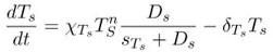
(2)

(3)

(4)

(5)

(6)

(7)

Eq. 1 represents the growth of CSCs through symmetric replication, the transition of nCSC to CSC, the transition of CSCs to nCSCs, killing of CSCs by CTCs, natural death of CSCs, and the death of CSCs by chemotherapy. Eq. 2 represents the growth of nCSCs through asymmetric replication, growth of the nCSC population through replication, the division of a CSC into two nCSCs, killing of nCSCs by nCSC-specific CTCs, natural death of nCSCs, and chemotherapy killing nCSCs. Eq. 3 represents the activation of naive CTCs (which become saturated) by mature CSC-specific DCs and the natural death of activated CSC-specific CTCs. Eq. 4 represents the activation of naive CTCs (which become saturated) by mature nCSC-specific DCs and the natural death of activated nCSC-specific CTCs. Eq. 5 represents the maturation of immature DCs when they encounter tumor cells with CSC-specific antigens and the killing of mature CSC-specific DCs. Eq. 6 represents the maturation of immature DCs when they encounter tumor cells with nCSC-specific antigens and the killing of mature nCSC-specific DCs. Eq. 7 represents the elimination of chemotherapy from the body. Host- specific parameters will be in the figure captions in the results section. These host-specific parameters vary based on patient and type of cancer.

3. Model 1: Tumor Inoculation with CSCs and nCSCs

In Model 1, the effect of tumor inoculation with CSCs and nCSCs on tumor size was studied. The tumor was inoculated with 50,000 CSCs or 50,000 nCSCs on Day 0. All cell populations were set to 0 in STELLA except for the cell population that was inoculated. The simulation in STELLA started on Day 12 (the time at which cancer cells would take root in a host) and ended on Day 25. Refer to Figure 6 for the baseline STELLA model.

4. Model 2: Dendritic Cell Vaccine Before Tumor Inoculation

In Model 2, the effects of a dendritic cell vaccine prior to tumor inoculation on tumor size were modeled. Dendritic cell vaccines were given on Day 0, Day 7, and Day 14. The tumor was inoculated on Day 22. There were four types of treatments simulated: no DC vaccination, DC vaccination with CSC-specific DCs and nCSC-specific DCs, DC vaccination with CSC-specific DCs, and DC vaccination with nCSC-specific DCs. In all simulations, a population of 10,000 CSCs and 90,000 nCSCs were used to inoculate the tumor. On each day the vaccine was given, 1 million mature DCs were added to the appropriate DC population for the DC vaccination with CSCs and the vaccination with nCSCs. For the mixed DC vaccine treatment, each vaccine contained 100,000 CSC- specific DCs and 900,000 nCSC-specific DCs. For the no treatment simulation, the tumor was only inoculated. The DC vaccines were sim- ulated in STELLA using the PULSE option. Prior to inoculation, all cell populations except for the appropriate mature DC population, if applicable, were set to zero. The inoculation of the tumor was modeled in STELLA with PULSE. The simulation was run from Day 0 to Day 49. Refer to Figure 7 for the STELLA model of Model 2.

5. Model 3: T-Cell Treatment After Tumor Inoculation

In Model 3, the effects of T-Cell treatment after tumor inoculation on tumor size were modeled. T-Cell treatment was given on Day 1, Day 8, and Day 15. There were four types of treatments: no treatment, mixed treatment with both CSC-specific and nCSC-specific CTCs, treatment with CSC-specific CTCs, and treatment with nCSC-specific CTCs. T-cell treatments consisted of 1,000,000 CSCs or nCSCs. For mixed treatment, treatments consisted of 50,000 CSC-specific CTCs and 950,000 nCSC-specific CTCs. All cell populations were set to 0 for Day 0. T-Cell treatments were modeled in STELLA using PULSE. The inoculation of the tumor on Day 8 was modeled in STELLA using PULSE which allowed for an inflow of 5,000 CSCs and 95,000 nCSCs. Refer to Figure 8 for the STELLA model of Model 3.

6. Model 4: Modeling the Effectiveness of T- Cell Treatment and Chemotherapy

In Model 4, there were six treatments modeled: no treatment, chemotherapy only, CSC-specific T-Cell treatment only, nCSC-specific T-cell treatment only, combined chemotherapy and CSC-specific T-cell treatment, and com- bined chemotherapy and nCSC-specific T-cell treatment. The tumor was inoculated on Day 0 with 5,000 CSCs and 95,000 nCSCs. All other populations were set to zero. For nCSC-specific T-cell treatment and CSC-specific T-cell treatment, one million activated CTCs were added to the appropriate population on Day 20 and 27 using PULSE. For chemotherapy treatment, one injection of 6,000 µg/ mL chemotherapeutic agent was given per day from days 20-24 and 27-31. Chemotherapy was modeled in STELLA using PULSE. For combined chemotherapy and T-cell treatment, the methods for modeling chemotherapy and T-cell treatment were used together in the STELLA model. Refer to Figure 9 for the STELLA model of Model 4.

7. Model 5: Modeling the Effectiveness of DC Vaccines and Chemotherapy

In Model 5, there were six treatments modeled: no treatment, chemotherapy only, mature CSC-specific DC vaccines only, nCSC-specific DC cell vaccines only, combined chemotherapy and CSC-specific DC vaccines, and combined chemotherapy and nCSC-specific DC vaccines. The tumor was inoculated on Day 0 with 5,000 CSCs and 95,000 nCSCs. All other populations were set to zero. For nCSC-specific DC vaccines and CSC-specific DC vaccines, one million mature DCs were added to the appropriate population on Day 20 and 27 using PULSE. For chemotherapy treatment, one injection of 6,000 µg/mL chemotherapeutic agent was given per day from days 20-24 and 27-31. Chemotherapy was modeled in STELLA using PULSE. For combined chemotherapy and DC vaccines, the methods for modeling chemotherapy and DC vaccines were used together in the STELLA model. Refer to Figure 9 for the STELLA model of Model 5.

8. Results and Discussion

For all models, the effectiveness of the treatment is shown in terms of tumor size. Tumor size was calculated by adding together the CSC population and nCSC population based on the results of the STELLA model and dividing by 100,000 using Excel [11]. All plots were created using Mathematica [22]. The host-specific parameters used for each model are reported in the figure captions. Refer to Table 1 for the meaning of each parameter and its value.

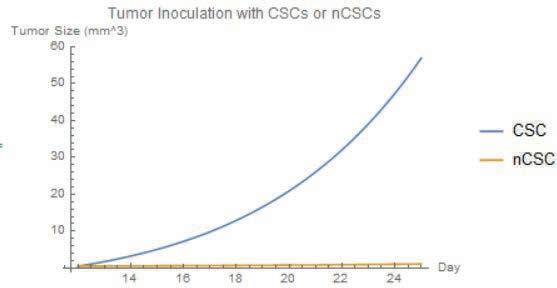
Figure 1. This figure shows the evolution of tumor size after inoculation with 50,000 CSCs or nCSCs. The

host-specific parameters are αS = 0.5 day-1 , δS = 0.2 day-1 , ρSP = 0.15 day-1 , αP = 0.2 day-1 , δP = 0.15 day-1 , αSP = 1.8 day-1 , and ρPS = 5.3 × 10−4 day-1 .

Inoculating a tumor with cancer stem cells leads to significant tumor growth, and inoculating a tumor with nCSCs leads to a significantly lower and comparatively negligible tumor growth in the same host-specific conditions (Fig. 1). These data support the finding that CSCs drive tumor growth [17].

DC vaccines prior to tumor inoculation are effective in slowing tumor growth when compared to no treatment (Fig. 2). The CSC-specific DC vaccine was most effective in reducing tumor size compared to the mixed DC vaccine and nCSC DC vaccine. The mixed DC vaccine was the second most effective in reducing tumor size.

CSC T-Cell treatment is significantly more effective in reducing tumor size compared to the mixed T-cell treatment, nCSC T-cell treatment, and no treatment (Fig. 3). In other words, activated CTCs cultured with mature dendritic cells that were pulsed with CSCs were more effective in reducing tumor growth compared to those pulsed with both CSCs or nCSCs or only nCSCs. All T-cell treatments were effective in reducing tumor size when compared to no treatment.

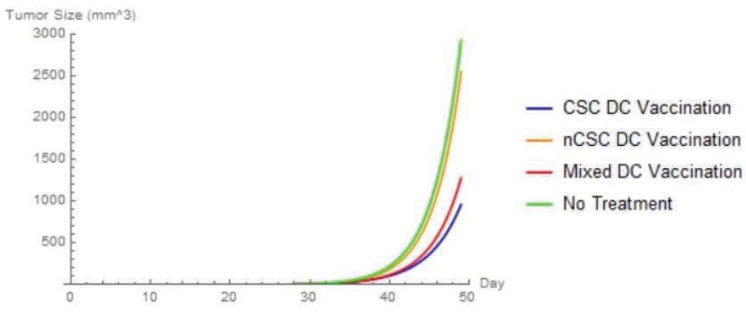
Figure 2. This figure shows the evolution of tumor size after dendritic cell vaccines with CSC-specific DCs and/or nCSC-specific DCs. The host-specific pa-

rameters are αS = 0.6 day-1 , δS = 0.2 day-1 , ρSP = 0.1 day-1 , αP = 0.2 day-1 , δP = 0.14 day-1 , αSP = 2.0 day-1, and ρPS = 4.4

× 10−4 day-1 .

Figure 3. This figure shows the evolution of tumor size after different T-cell treatments and no treat-

ment. The host-specific parameters are αS = 0.7, δS = 0.19 day-1 , ρSP = 0.24 day-1 , αP = 0.2 day-1 , δP = 0.1 day-1 , αSP = 2.8 day-1, and ρPS = 1.3 × 10−4 day-1 .

Figure 4. This figure shows the evolution of tumor size after T-cell treatments, chemotherapy, and combined T-cell and chemotherapy treatments. The

host-specific parameters are αS = 0.5 day-1 , δS = 0.2 day-1 , ρSP = 0.15 day-1 , αP = 0.2 day-1 , δP = 0.15 day-1 , αSP = 1.8 day-1 , and ρPS = 5.3 × 10−4 day-1 .

Chemotherapy is a more effective treatment for treating tumors compared to only CSC T-cell treatment or nCSC T-cell treatment (Fig. 4). The combined chemotherapy treatments and T-cell treatments were most effective in reducing tumor size. CSC T-cell treatment with chemotherapy was the most effective followed by combined nCSC T-cell treatment with chemotherapy and chemotherapy only. All treatments had the same tumor size until Day 20, when the first chemotherapy and/or immunotherapy treatment was given. All treatments involving chemotherapy saw an oscillating decrease in tumor size before an increase in tumor size after the last day of chemotherapy treatment. All treatments with chemotherapy had similar tumor size at the end of the simulation which was significantly less than treatments without chemotherapy. Treatments that did not involve chemotherapy saw a significant increase in tumor size, which continued until the end of the simulation.

Figure 5. This figure shows the evolution of tumor size after DC vaccines, chemotherapy, and combined chemotherapy treatment and DC vaccines. The

host-specific parameters are αS = 0.5 day-1 , δS = 0.2 day-1 , ρSP = 0.15 day-1 , αP = 0.2 day-1 , δP = 0.15 day-1 , αSP = 1.8 day-1 , and ρPS = 5.3 × 10−4 day-1 .

Treatments with chemotherapy, especially those combined with immunotherapy treatments, are more effective in reducing tumor size compared to no treatment or only immunotherapy treatment (Fig. 4 and 5). The combined treatment with CSC-specific DC Vaccine treatment and chemotherapy was most effective in reducing tumor size (Fig. 5). The combined treatment with nCSC-specific DC vaccine treatment and chemotherapy was the second most effective treatment for reducing tumor size. However, all chemotherapy treatments had a very similar tumor size at the end of the simulation. In addition, the immunotherapy treatments and no treatment had a very similar tumor size by the end of the simulation.

All results suggest that immunotherapy treatments targeting CSCs are the most effective in reducing tumor growth. After CSC-specific immunotherapy treatment, T-cell receptors will recognize CSC-specific antigens, bind to antigen peptides on MHC Class I molecules on CSCs, and kill the CSCs through the release of cytokines, cytotoxic granules, or the FasL ligand. CSC-specific dendritic cell vaccines and T-cell adoptive therapy allow the immune system to directly target and kill CSCs. In contrast, nCSC-specific dendritic cell vaccines and T-cell adoptive therapy are less effective in reducing tumor size, since cytotoxic T-cells will kill nCSCs and lead to comparably negligible tumor growth due to lower renewal rate and inability to differentiate [17] (Fig. 1).

9. Conclusions

In this paper, a computational model was used to study how dendritic cells and cytotoxic T-cells impact tumor-immune interaction with CSCs and nCSCs. The model found that tumor inoculation with CSCs produced larger tumors compared to tumors inoculated with nCSCs. CSC-specific DC vaccines are more effective in reducing tumor growth than mixed or nCSC-specific DC vaccines (Fig. 2). CSC-specific T-cell treatment was more effective in reducing tumor growth than mixed or nCSC-specific T-cell treatment (Fig. 3). Cancer treatments involving chemotherapy were most effective in reducing tumor growth compared to immunotherapy treatments alone (Fig. 4 & 5). However, combined chemotherapy and immunotherapy treatments (CSC-specific DC vaccines or CSC-specific T-cell treatment) were most effective in reducing tumor size. T-cell treatment was more effective in reducing tumor size after inoculation compared to dendritic cell vaccines. The CSC-specific T-cell treatment and chemotherapy treatment was the most effective treatment overall for reducing tumor growth after inoculation. This model could be improved to include the role of T-helper cells in activating cytotoxic T-cells [19] [17]. Mature den- dritic cells present antigens to both cytoxic T-cells and T-helper cells through MHC Class I and MHC Class II [17]. T-helper cells give cytotoxic T-cells a costimulatory signal that is needed for T-cells to become activated as well as proliferate [17]. The model could add the role of T-regulatory cells that inhibit T-cell activation and proliferation [16][17][19]. In the model, exponential growth was assumed that may not occur in vivo. Some cancer cells that were inoculated may have been destroyed in vivo prior to the cancer cells taking root which may be a potential source of error. In addition, DC cells can lead to death of CSC and nCSCs but was not considered in the model, since the effect on the cell populations is considered negligible compared to cell death caused by CTCs. Tumors are also believed to affect the maturation of dendritic cells and cytotoxic T-cells, which was not considered in the model as the effects are currently unclear. The proposed computational model could have large implications in studying immunotherapy effectiveness and combined immunotherapy and chemotherapy treatments for many types of cancer including pancreatic cancer, breast cancer, squamous head and neck cancer, and brain tumors. The host-specific parameters and chemotherapy treatment parameters can be modified for a patient or a type of can-

cer. In addition, the renewal rate of CSCs and nCSCs can be modified for each type of cancer.

10. Acknowledgements

The author thanks Mr. Robert Gotwals for his assistance with this work. In addition, I would like to thank the Broad Street Scientific editors.

11. References

[1] Al-Tameemi, M., Chaplain, M., d’Onofrio, A. (2012). Evasion of tumours from the control of the immune system: consequences of brief encounters. Biology direct, 7(1), 31.

[2] Castiglione, F., Piccoli, B. (2006). Optimal control in a model of dendritic cell transfection cancer immunotherapy. Bulletin of Mathematical Biology, 68(2), 255-274.

[3] Cheng, M., Chen, Y., Xiao, W., Sun, R., Tian, Z. (2013). NK cell-based immunotherapy for malignant diseases. Cellular molec- ular immunology, 10(3), 230.

[4] Dashti, A., Ebrahimi, M., Hadjati, J., Memarnejadian, A., Moazzeni, S. M. (2016). Dendritic cell based immunotherapy using tumor stem cells mediates potent antitumor immune responses. Cancer letters, 374(1), 175-185.

[5] DePillis, L. G., Eladdadi, A., Radunskaya, A. E. (2014). Modeling cancer-immune responses to therapy. Journal of pharmacokinetics and pharmacodynamics, 41(5), 461-478.

[6] de Pillis, L. G., Radunskaya, A. (2003). A mathematical model of immune response to tumor invasion. In Computational Fluid and Solid Mechanics 2003 (pp. 1661-1668). Elsevier Science Ltd.

[7] de Pillis, L. G., Radunskaya, A. E., Wiseman, C. L. (2005). A validated mathematical model of cell-mediated immune response to tumor growth. Cancer research, 65(17), 7950-7958.

[8] Kirschner, D., Panetta, J. C. (1998). Modeling immunotherapy of the tumor–immune interaction. Journal of mathematical biology, 37(3), 235-252.

[9] Kuznetsov, V. A., Makalkin, I. A., Taylor, M. A., Perelson, A. S. (1994). Nonlinear dynamics of immunogenic tumors: parameter estimation and global bifurcation analysis. Bulletin of mathematical biology, 56(2), 295-321.

[10] Mahasa, K. J., Ouifki, R., Eladdadi, A., de Pillis, L. (2016). Mathematical model of tumor–immune surveillance. Journal of theoretical biology, 404, 312-330. [11] Microsoft Excel [Software] Available from https:// products.office.com/en-us/excel.

[12] de Mingo Pulido, A., Ruffell, B. (2016). Immune regulation of the metastatic process: implications for therapy. In Advances in cancer research (Vol. 132, pp. 139-163). Academic Press.

[13] Morisaki, T., Matsumoto, K., Onishi, H., Kuroki, H., Baba, E., Tasaki, A., Tanaka, M. (2003). Dendritic cell-based combined immunotherapy with autologous tumor-pulsed dendritic cell vaccine and activated T cells for cancer patients: rationale, current progress, and perspectives. Human cell, 16(4), 175-182.

[14] Ohaegbulam, K. C., Assal, A., Lazar- Molnar, E., Yao, Y., Zang, X. (2015). Human cancer immunotherapy with antibodies to the PD-1 and PD-L1 pathway. Trends in molecular medicine, 21(1), 24-33.

[15] Palucka, K., Banchereau, J. (2012). Cancer immunotherapy via dendritic cells. Nature Reviews Cancer, 12(4), 265.

[16] Rhodes, A., Hillen, T. (2019). A Mathematical Model for the Immune-Mediated Theory of Metastasis. bioRxiv, 565531.

[17] Sigal, D., Przedborski, M., Sivaloganathan, D., Kohandel, M. (2019). Mathematical modelling of cancer stem cell-targeted immunotherapy. Mathematical Biosciences, 318, 108269.

[18] STELLA Architect (Version 1.6.2) [Software] Available from https://www.iseesystems.com/store/products/ stellaarchitect.aspx.

[19] Qomlaqi, M., Bahrami, F., Ajami, M., Hajati, J. (2017). An extended mathematical model of tumor growth and its interaction with the immune system, to be used for developing an optimized immunotherapy treatment protocol. Mathematical biosciences, 292, 1-9.

[20] Vigneron, N. (2015). Human tumor antigens and cancer immunotherapy. BioMed research international, 2015.

[21] Wilson, S., Levy, D. (2012). A mathematical model of the enhancement of tumor vaccine efficacy by immunotherapy. Bulletin of mathematical biology, 74(7), 14851500.

[22] Wolfram Mathematica (12.0 Student Version) [Software] Available from https://www.wolfram.com/mathematica/.

[23] Yu, J. L., Jang, S. R. J. (2019). A mathematical model of tumor-immune interactions with an immune checkpoint inhibitor. Applied Mathematics and Computation, 362, 124523.

12. Appendix

Figure 6: Baseline STELLA Model for Tumor Inoculation (Model 1)

Figure 7: STELLA Model for DC Vaccines (Model 2)

Figure 8: STELLA Model for T-Cell Adoptive Therapy (Model 3)

Figure 9: STELLA Model for Chemotherapy and Combined Treatments (Models 4 and 5)

THE COSMIC RADIATION SHIELDING PROPERTIES OF LUNAR REGOLITH

Eleanor Murray

Abstract

Lunar regolith is the most accessible material for use as radiation shielding for human habitation on the Moon. This study aims to determine the thickness of lunar regolith shielding necessary to protect humans from cosmic radiation and its secondaries, including neutrons. We measured the percentage of thermal neutrons that passed through prepared LHS-1 Lunar Highlands Simulant samples of different thicknesses using the Neutron Powder Diffraction Facility at the PULSTAR Reactor of NC State University, prepared for a neutron transmission experiment. In addition, we modeled an analogue of the experiment using GEANT4 software. We present the results of the neutron experiments as well as preliminary results of the necessary thickness at which the radiation dose will drop to safe levels based on GEANT4 simulations of the interactions of galactic cosmic rays with the lunar regolith-like material.

1. Introduction

As NASA prepares for a Moon landing in 2024 with the Artemis program, leading towards “sustainable missions by 2028” [1], the In-Situ Resource Utilization (ISRU) of lunar regolith will be integral. Particularly on a large scale, the costs of ISRU will need to be balanced with the potential costs of transporting materials from Earth. One potential cost is that of launching radiation shielding materials to the Moon. However, this cost could be mitigated by using a material readily available on the Moon as radiation shielding: the lunar regolith. Eckart found that a 1 meter layer of lunar regolith would prevent crew members from receiving more than about 3 cSV of radiation from each solar particle event [2]. The main types of radiation on the Moon are galactic cosmic rays (GCR) and solar particle events (SPE). Galactic cosmic rays are a constant source of radiation, while solar particle events occur only occasionally but expose astronauts to a greater momentary amount of radiation. During an SPE, astronauts can stay in an area with more shielding, but GCR is harder to protect against since it is constant [3]. The protons in the SPE are also “fairly easy to stop, compared to GCR” [4]. More research is necessary in order to protect astronauts on long-term missions from the GCR.

2. Lunar Regolith as Radiation Shielding

On Earth, humans are protected from excessive amounts of solar radiation by Earth’s magnetic field. The Moon’s magnetic field is much weaker [5], so radiation shielding will be necessary for human habitation. Eckart [2] writes that calculations have found layers of lunar regolith 50-100 cm deep to be sufficient in decreasing radiation doses from the GCR and SPE to acceptable levels [6]. Miller [6] found that less than 50 cm of lunar regolith should be enough to stop the most damaging and common galactic cosmic rays (GCR) as well as protons from solar particle events (SPE). This study found that lunar regolith, and several simulants are comparable to aluminum in their radiation-shielding properties by measuring the dose reduction per unit areal density [6]. However, this study did not investigate the impact of neutrons in this measurement. As galactic cosmic rays impact the lunar surface, they produce secondary radiation, which includes neutrons. Both the protons from above and the neutrons from below will pose major risks to astronauts [7]. A greater understanding of the radiation shielding properties of lunar regolith is essential to planning potential lunar habitats that will attenuate radiation to safe levels.

3. Safe Limits of Radiation

Determing a safe level of radiation is difficult as studies use varying units. A gray is a measure of how much energy was absorbed; one gray is equal to one joule per kilogram. Sieverts are similar but relate to the expected amount of biological damage; the conversion between grays and sieverts depends on the type and energy of the radiation. Globus and Strout surveyed the literature and found that in the context of orbital space settlements, the general population should not receive more than 20 millisieverts per year [4]. The World Nuclear Association states that less than 100 millisieverts per year is harmless [8]. In addition, NASA lists 500 milligray-equivalents as the limit of radiation to the blood-forming organs of astronauts per year[9]. The radiation on the moon comes from Solar Particle Events (SPE), which are occasional but deliver large amounts of radiation, and Galactic Cosmic Rays (GCR), which are constant, deliver smaller amounts of radiation, come from far away galaxies as opposed to the Sun, and are harder to shield against than SPE. When these charged particles impact the regolith of the Moon, nuclear reactions occur and produce free neutrons, adding to the radiation dose humans would receive [7].

Previous research, such as the Lunar Exploration Neutron Detector (LEND), took data from approximately 50 kilometers above the moon instead of at its surface [10]. The LEND examined albedo neutrons, or the neutrons that are created in the lunar surface and then bounce back towards space [11], instead of the neutrons that are created in the regolith and move downwards where they would contribute to the radiation dose experienced by astronauts.

During the Apollo 17 mission, astronauts successfully deployed the Lunar Neutron Probe Experiment (LNPE). This probe consisted of a 2-meter-long rod that was placed in the lunar regolith to measure the rates of capture of low energy neutrons at various depths. This experiment is one of the few measurements of neutrons on the lunar surface. However, the experiment was designed with low energy neutrons in mind, while the radiation dose from neutrons also includes high energy neutrons. The LNPE report also included only preliminary data; and calibration of the data had not been completed [12].

These limitations on the available data require GEANT4 simulations as well as an empirical experiment to model the radiation dose on the Moon as it varies with depth of lunar regolith.

5. Lunar Regolith Simulants

Lunar regolith is difficult to obtain, so most research on lunar regolith involves JSC-1 lunar regolith simulant, which is produced by NASA. We utilized LHS-1 Lunar Highlands Simulant since its availability is higher than that of JSC-1 Lunar Regolith Simulant. However, their percent compositions are roughly similar, as shown in Table 1.

Table 1. Percent Composition by weight of oxides. Data compiled from references [17-19].

OxideLunar Regolith (Highlands) Na .6 LHS-1 JSC-1

2.30 2.7

Mg 7.5 Al 24.0 Si 45.5 Ca 15.9 Ti .6 Fe 5.9 11.22 9.01 26.24 15.02 44.18 47.71 11.62 10.42 .79 1.59 3.04 10.79

Since an estimate of the linear stopping power of a compound can be made by assuming linear stopping power is additive [13], the linear stopping powers of lunar regolith, JSC-1 Lunar Regolith Simulant, and LHS-1 Lunar Highlands Simulant should be roughly equal. 6.1 - Methodology

We investigated the feasibility of using lunar regolith as shielding against neutrons from the radiation environment of the Moon. LHS-1 Lunar Highlands Simulant was used as a proxy for lunar regolith. The simulant was contained by aluminum boxes (show schematically in Fig. 1) that were manufactured on the NC School of Science and Mathematics campus.

Figure 1. Diagram of Aluminum Boxes for Samples

Ten samples that are two inches by two inches across with varying thicknesses x were prepared. The smallest thickness was ¼ inch, and the largest thickness was 2 ½ inches, increasing in ¼ inch increments.

Figure 2a. Image of Neutron Powder Diffraction Facility. Image credit: Mr. Scott Lassell [14]

The samples were taken to the NC State PULSTAR reactor, and were experimented on at the Neutron Powder Diffraction Facility (shown in Figure 2a) prepared for a transmission experiment. A diagram of the neutron transmission experiment carried out on these samples is shown in Figure 2b. The de Broglie wavelength of the neutrons was 1.478 angstroms [15], corresponding to a kinetic energy of approximately 0.03745 electron-volts. The number of neutrons that hit the detector was measured both without a target and after passing through the samples.

Figure 2b. Diagram of Neutron Transmission Experiment

6.2 - Results

The equation (N/N0)=e-b*t was used to analyze the data, where N is the number of neutrons that passed through the sample in one minute, N0 is the intensity of neutrons in the initial beam in one minute, b is a constant that represents the probability any one neutron will interact per centimeter, and t is the thickness of the lunar regolith simulant sample in centimeters. N=3168e(-.18*t) was found to fit the data, so for any one neutron, there is an 18% chance that it will interact per centimeter of lunar regolith simulant. Figure 3 shows the thickness of lunar regolith simulant in centimeters on the x-axis and the neutron fluence over one minute per cm2 on the y-axis.

Figure 3. Neutron Fluence vs. Thickness of Sample

The data were also linearized to give the equation y=-.18*t+ln(N0) where y=ln(N). The slope of this graph (Fig. 4) again shows that there is an 18% chance that any one neutron will interact per centimeter of lunar regolith simulant.

Figure 4. ln(Neutron Fluence) per cm2 vs. Thickness of Sample

The attenuation length is defined as the depth of the material where the intensity of the radiation decreases to 1/e of the initial intensity [16]. The attenuation length of the LHS1 lunar regolith simulant is approximately 6.51 g/cm2. The mass attenuation coefficient is equivalent to the chance that any one neutron will interact per centimeter divided by the density of the material [13]. In this case, the mass attenuation coefficient is 0.15 cm2/g.

7. Method 2: GEANT4 Simulations

7.1 - Methodology

GEANT4 simulation software was run in batch mode for each thickness, and a short Python program was used to analyze the output to count the number of neutrons that passed through the material. Figure 5 below shows a side view of this scenario, where the blue rectangle represents the material defined to be similar by percent composition to LHS-1 Lunar Highlands Simulant, the gray bar is “Shape 2,” the green tracks show the neutrons, and the neutrons start from the middle of the left side of the material. Only 100 neutrons are shown for clarity. Neutrons were counted as having passed through the material if they hit Shape 2, which was a thin cylinder modeled as bone with a diameter of 1.27 cm, centered at the position of the point source and thickness x centimeters from the point source.

Figure 5. GEANT4 Simulation of Neutrons Passing Through the Material.

7.2 - Results

Figure 6 shows the number of neutrons per centimeter squared that passed through the material vs. the thickness of the material in centimeters.

According to the equation, (N/N0)=e-bt, there is approximately a 12% chance per centimeter that any particular neutron will interact with the material. The attenuation length is 9.8 g/cm2, and the mass attenuation coefficient is 0.10 cm2/g. Figure 7 shows the same data, but linearized, so that y=-bt+ln(N0), and y=ln(N). Here, b equals approximately 0.12, so there is a 12% chance per centimeter that a neutron will interact with the lunar regolith simulant.

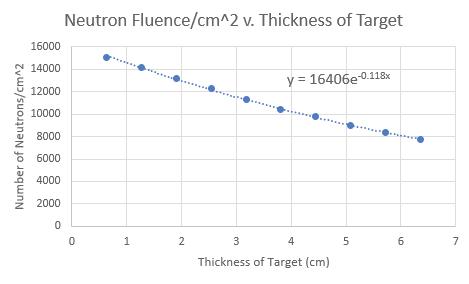
Figure 6. Number of Neutrons/cm2 vs. Thickness of Material.

Figure 7. ln(Number of Neutrons) vs. Thickness of Material.

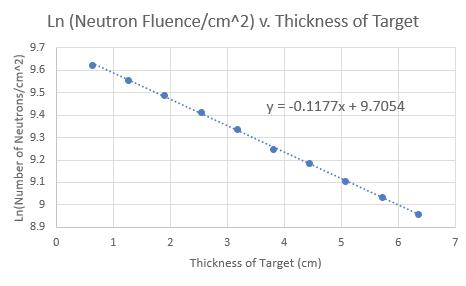
The percent difference between the value of b, or the percent chance that any one neutron will interact per centimeter, found with the nuclear reactor (18%) and the value found with GEANT4 simulations (12%) is 40%. The percent difference in the attenuation lengths is 36%, and the percent difference in the mass attenuation coefficients is 40.%. A possible source of this error is the differences in the geometry of the detectors; the neutron detector at the nuclear reactor is set approximately 1 meter behind the sample while the detector in GEANT4 is set directly behind the sample.

8. Discussion

Based on the empirical method described earlier, about 6.5 g/cm2 is the attenuation length of 0.03745 eV neutrons in LHS-1 Lunar Highlands Simulant. For any one neutron, there is about an 18% chance that it will interact with the simulant per centimeter. However, a similar experiment modeled in GEANT4 found a 12% chance per centimeter that any one neutron will interact with the simulant, and an attenuation length of 9.8 g/cm2. The percent difference between the chances each neutron will interact per centimeter is 40%, and the percent difference between the attenuation lengths is 36%. A possible explanation for the discrepancy is the differences in geometry of the two experiments; in the nuclear reactor experiment, the neutron detector was 135 centimeters [14] away from the neutron source, while in the GEANT4 experiment, the detector was set right behind the sample with the neutron source set at the front of the sample. Therefore in the nuclear reactor experiment, the distance between the neutron source and detector was always 135 centimeters, while in GEANT4, the distance between the neutron source and detector varied between 0.635 centimeters and 6.35 centimeters in 0.635 centimeter increments. Additionally, the aperture of the collimated neutron beam at the reactor had an internal diameter of 1.3 centimeters [14], while in GEANT4, the neutrons came from a collimated point source. Other possible sources of the discrepancy are the slightly different percent compositions between the LHS-1 Lunar Highlands Simulant used in the nuclear reactor experiment and the material used in the GEANT4 experiment. In the future, more simulations can be done with protons simulating the GCR, including neutron secondaries, to find the thickness of lunar regolith at which the radiation dose drops to safe levels.

9. Conclusion

Thermal neutrons have an 18% chance per centimeter of interacting with LHS-1 Lunar Highlands Simulant, with an attenuation length of 6.51 g/cm2 and a mass attenuation coefficient of .15 cm2/g. The radiation shielding properties of lunar regolith should be similar to LHS-1 Lunar Highlands Simulant since their percent compositions are similar. This information is useful to the designs of prospective lunar habitats. Simulations in GEANT4 show reasonable agreement with the thermal neutron transmission experiment. However, thermal neutrons are not a great model for cosmic radiation, so GEANT4 will be used to model the interactions of lunar regolith with the full radiation environment of the Moon in order to determine the thickness of lunar regolith at which the radiation dose falls to safe levels for long-term human habitation.

10. Acknowledgements

The author would like to thank their mentor, Dr. Jonathan Bennett, the physics chair at the North Carolina School of Science and Mathematics (NCSSM), Mr. Benjamin Wu for his assistance with coding a program for data analysis, as well as Ms. Bec Conrad, the manager of the Fabrication and Innovation Laboratory at NCSSM, and the NCSSM Foundation. Additionally, the author would like to thank Dr. Quinsheng Cai and Mr. Scott Lassell for their assistance in utilizing the PULSTAR Reactor at North Carolina State University, the developers and forum of GEANT4, as well as the Center for Lunar and Asteroid Surface Science (CLASS) Exolith Lab for providing the

LHS-1 Lunar Highlands Simulant used in this study.

11. References

[1] “What is Artemis?” NASA.gov, https://www.nasa. gov/what-is-artemis. Accessed 28 Oct. 2019.

[2] Eckart, Peter. The Lunar Base Handbook. The McGraw-Hill Companies, Inc., 1999

[3] Blanchett, Amy and Laurie Abadie. “Space Radiation Won’t Stop NASA’s Human Exploration.” NASA.gov, 12 Oct. 2017, https://www.nasa.gov/feature/space-radiation-won-t-stop-nasa-s-human-exploration

[4] Globus, Al and Joe Strout. “Orbital Space Settlement Radiation Shielding”. National Space Society, April 2017.

[5] Halekas, Jasper S. and Robert P. Lin. “Determining Lunar Crustal Magnetic Fields and Their Origin”. Lunar and Planetary Institute, https://www.lpi.usra.edu/meetings/ LEA/presentations/tues_pm/2_Halekas_Lunar_Crustal_ Magneti_Breakout1.pdf. Accessed 27 Oct. 2019

[6] Miller J., et al. 2009. “Lunar soil as shielding against space radiation”, page 167. Radiation Measurements

[7] Barry, Patrick L. “Radioactive Moon.” NASA.gov, 8 Sept. 2005, https://science.nasa.gov/science-news/science-at-nasa/2005/08sep_radioactivemoon

[8] “What is Radiation?” World Nuclear Association, https://www.world-nuclear.org/information-library/safety-and-security/radiation-and-health/radiation-and-life.aspx. Accessed 13 Aug. 2019.

[9] NASA Space Flight Human-System Standard: Volume 1, Revision A: Crew Health. NASA.gov, pp. 22, 30 July 2014. https://standards.nasa.gov/standard/nasa/nasa-std3001-vol-1. Accessed 22 Oct. 2019

[10] “Building the LRO Spacecraft.” NASA, https://lunar. gsfc.nasa.gov/spacecraft.html. Accessed 3 Oct. 2019

[11] Litvak, M. L. et al. “Global maps of lunar neutron fluxes from the LEND instrument.” Journal of Geophysical Research, vol. 117, June 2012, pp. 1-2, https://www. researchgate.net/publication/235979801_Global_maps_ of_lunar_neutron_fluxes_from_the_LEND_instrument. Accessed 28 Oct. 2019

[12] Woolum, Dorothy S. et al. “The Apollo 17 Lunar Neutron Probe Experiment.” Astrophysics Data System, http://adsabs.harvard.edu/full/1973LPI.....4..793W. Accessed 28 Oct. 2019 [13] Knoll, Glenn F. Radiation Detection and Measurement, page 41. 3rd. ed., John Wiley and Sons, Inc., 2000 [14] Lassell, Scott. Personal interview. 23 Oct. 2019

[15] “Neutron Powder Diffraction Facility.” NCSU. edu, https://www.ne.ncsu.edu/nrp/user-facilities/neutron-diffraction-facility/.

[16] X-Ray Attenuation Length. http://henke.lbl.gov/optical_constants/atten2.html. Accessed 4 Aug. 2019

[17] “LHS-1 Lunar Highlands Simulant Fact Sheet.” UCF. edu, Mar. 2019, http://sciences.ucf.edu/class/wp-content/ uploads/sites/58/2019/02/Spec_LHS-1.pdf

[18] McKay, David S. et al. “JSC-1: A New Lunar Soil Simulant.” USRA.edu, 1994, https://www.lpi.usra.edu/lunar/ strategies/jsc_lunar_simulant.pdf

[19] Turkevich, A. L. “The average chemical composition of the lunar surface.” NASA Astrophysics Data System, http://adsabs.harvard.edu/full/1973LPSC....4.1159T. Accessed 17 May 2019.

MODELING THE GRAVITATIONAL LENS OF THE EINSTEIN RING MG1131+0456

Nathaniel S. Woodward

Abstract

We present the results of modeling the distribution of mass in the elliptical lensing galaxy of the Einstein ring MG1131+0456 using numerical and computational modeling methods. We applied two mass models of varying complexity to this system: a point mass and a singular isothermal sphere. In constructing these models, we relied on image construction through ray-tracing. Results from the ray tracing method qualitatively agree with both the literature and the observed radio imaging of MG1131. Total mass derived from the ray tracing model was within the range predicted by previous models. Current work aims to extend the ray-tracing model to include a singular isothermal ellipsoid as well as applying this model to gravitational lenses that have not been analyzed.

1. Introduction

Gravitational lensing is a phenomenon predicted by Einstein’s general theory of relativity where the path of light is determined based on the curvature of the spacetime. Gravitational lensing is a powerful tool when applied to problems in modern physics and has allowed physicists to measure universal constants such as the Hubble constant and the deceleration parameter at a high degree of accuracy, which quantify the expansion and deceleration of the expansion of the universe, respectively [1][2]. Gravitational lensing has also allowed physicists to determine distributions of dark matter in galaxies and throughout the universe and construct more accurate models of galaxies [3]. In recent years, gravitational lensing analysis has been conducted primarily through the comparison of observation studies and computational studies that rely on mass models to represent the lensing object. In this paper we will examine the gravitational lens MG1131+0456 and aim to calculate the mass distribution and total mass. We will compare our results directly to those of Chen et al. to verify our model [4]. After testing our model against the literature, we hope to determining the total mass and mass distribution of systems that have not been studied.

1.1 – MG1131+0456 as a gravitational lens

MG1131+0456 is an extensively studied gravitationally lensed system and because of this we can characterize it based on the previous literature. The literature suggests that the source of MG1131+0456 is a distant quasar within the range of 3500 to 4200 Mpc [6]. The radiation emitted by this quasar is believed to be lensed by a massive elliptical galaxy and the resulting images have been analyzed in the infrared and radio wave wavelength [5][6]. The exact orientation of this galaxy has been debated in the literature and because of the uncertainty, we will work to examine a variety of orientations in our model. Figure 1 displays MG1131+0456 in the radio wavelength as recorded in the CfA-Arizona Space Telescope LEns Survey of gravitational lenses (CASTLeS) [7]. The image of MG1131+0456 in the radio wavelength expresses two distinct features: a near complete Einstein ring and two distinct compact images. Previous studies have utilized these features to suggest the source image may be composed of two compact components [5]. One of these components is collinear with the lens and the observer and is lensed into an Einstein ring. The other compact component is slightly offset from the line connecting the observer and lens and as a result, is lensed into the two compact multiple images. We will conduct our gravitational lensing analysis under the assumed geometry of the source where the quasar is composed of two distinct compact components.

Figure 1. The gravitational lens MG1131+0456 in radio imaging. Credit: Hewitt et al. 1988. [5]

1.2 – Distance Values

The distance to the source has been debated throughout

the literature, but based on redshift data, we can construct a range of possible distances. Work by Tonry et al. estimated a source redshift ranging from z = 1.9 to z = 5 [6]. We assumed the predictions by Tonry et al. as bounds for all possible redshifts for the source quasar. We first solve the equation for recession velocity v from the relativistic Doppler effect, shown in Eq. 1 where γ is the Lorentz factor and z is the redshift.

(1)

From the range of redshifts, we use the source redshift to calculate a recession velocity using Eq. (2).

(2)

After calculating a recession velocity, we can apply Hubble’s law in Eq. 3 with a Hubble constant value of 69.8 km/s/Mpc from the results of Freedman et al. [8] to determine the distance to the source.

(3)

Using Eq. 2 and Eq. 3, we computed a source distance in the range of 3500 to 4200 Mpc. While the redshift of the source is debated, the redshift of the lensing object is agreed upon as 0.84 [6]. Using the same procedures, we calculated a distance to the lens of 2400 Mpc [6]. We will refer to the distance to the source and the distance to the lens as Ds and Dl respectively.

Figure 2. We can see that under the thin lens approximation where the lensing object is represented as a plane, our distance approximation holds. In addition to displaying distance values, this diagram also shows the angular values that describe a lensing system, where θ is the angle of observance, β is the angular deviance of the source from the optical axis,

andˆα and α are the deflection vector and reduced

deflection angle, respectively. Credit: [9]

We also define a variable Dls that represents the distance between the lens and the source. Under the thin lens approximation, which assumes spacetime to be Cartesian everywhere except the lensing plane, we assumed that Ds − Dl = Dls. As shown in Figure 2, under the thin lens approximation, this assumption holds.

2. Materials and Methods

2.1 – Preliminary Point Mass Model

Determining a mass model for a lensing object is an integral part of the lensing analysis. First we conducted an analysis modeling the lensing galaxy as a point mass. The aim of this analysis was simply to validate that our distance values from the literature for the lensing system were approximately correct. In creating our point mass model for the lensing galaxy, we set all distance values equal to the values determined from the literature.

Examining the data from Hewitt et al. [5], shown in Figure 1, we designated the two compact components as multiple images and computed the Einstein ring radius. The Einstein ring angular radius is a characteristic of a lensing object and can be calculated for a point mass model by Eq. 4, where θE is the Einstein ring angular radius and θ+ and θ− are angular deviation of the positive and negative multiple images respectively [9]:

(4)

The simplicity of the point mass model allowed us to iterate through possible distances within the range of 3482 Mpc to 4183 Mpc and calculate a system mass using Equation 5:

(5)

Under the assumption that Ds − Dl = Dls, we can reduce Eq. (5) to;

(6)

By nature of the point mass model, there exists a possible mass such that at every point within the source distance range an Einstein ring and multiple images would form to match the data. This yields a range of possible masses calculated from the bounds of the distance range. With a known Einstein ring angular radius and lens distance, we are left one free parameter of the source distance. We calculate the total mass of our point mass model using Eq. 6 by iterating through source distances derived from Tonray et al.’s redshift predictions. Our analysis predicted a mass in the range of 2.9 * 1041 kg to 4.0 * 1041 kg. A ray tracing diagram of our point mass model is shown in Figure 3 which displays the distance range and shows light rays emitted from two distinct compact components. Our predicted values from the point mass model are within ≈ 20% compared to the result of 5.1 * 1041 kg predicted by Chen et. al. [4].

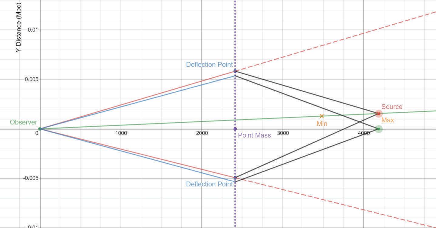
Figure 3. The ray tracing diagram above displays how the literature suggests the lensing system MG1131+0456 is composed. There are two luminous points of the source quasar representing the compact components of the source. Rays of light travel from these points to the lensing plane and some of these rays are deflected to reach the observer. The diagram also displays the minimum and maximum distance values for the source quasar which are labeled ”Min” and ”Max.” Dashed lines correspond to locations of virtual images for the multiple images.

2.2 – SIS Mass Model

After completing our rudimentary analysis using the point mass model, we extended our model to describe an SIS mass distribution. A Singular Isothermal Sphere model, or SIS, is a simple, but effective model for gravitational lensing systems. An SIS model represents a galaxy as a sphere of gas in hydrostatic equilibrium[9]. In this model, the motions of particles in the spherical gas cloud in hydrostatic equilibrium are analogous to the orbital motion of objects in the galaxy. Equations that describe an SIS model are derived directly from the ideal gas law and the equation of hydrostatic equilibrium [9]. The SIS model and its deflection of light rays are shown in Figure 4.

The SIS mass model allows us to include a non-uniform mass distribution which is fundamental to an accurate approximation of a galaxy. Every parameter of the SIS mass model depends on the velocity dispersion or σ. The velocity dispersion is analogous to the temperature of a cloud of particles in hydrostatic equilibrium, but for the motion of planets and stars in a galaxy, it describes the characteristic speed of masses in motion [9]. The velocity dispersion can be treated as a free parameter, but often is estimated to 225 km/s. With the velocity dispersion known or parameterized, we can calculate properties of an SIS mass model using the equations [9]:

(7)

(8)

(9)

The mass within radius R or M(R) is a function of the impact radius R, which is the radial distance to the center of lens from the point a ray of light impacts the lensing plane, and grows without bound as R approaches infinity (shown in Eq. 7). The mass density within a radius R or Σ(R) is inversely proportional to R and therefore predicts a singularity of infinite density as R approaches zero (shown in Eq. 8). By limiting the upper bound of R to some radial extent, we ensure that the total mass is finite, but a finite core density can only be achieve through extending to a more complex mass model. A key characteristic of the SIS model is shown in Eq. 10, a deflection angle independent of R.

(10)

Figure 4. A source object of varying brightness is shown to be emitting light which impacts the lensing plane at arbitrary points. We can see that the lens plane contains a spherical lensing object which deflects the incident rays of light. Some of the deflected rays of light impact the observer and become images of the source.

2.3 – Ray Tracing SIS Model

We chose to devise a new method to characterize our lensing system by tracking the path of individual light rays as they impacted the lensing plane. We predict an image based off the light rays calculated to impact the observer. In creating this model, we chose to work primarily with the SIS model as it reduces the complexity of the ray tracing model and is shown to be a reasonable model for an elliptical galaxy. The SIS lowers complexity because it is spherically symmetric, so to compute light deflection we only require the impact radius.

First we defined a source matrix where every cell has an assigned unitless brightness value. We then convert these brightness values into pixels by converting all brightness values into percent maximum brightnes. The source matrix that we use to construct the source plane and the corresponding source plane are shown in Figure 5.

Figure 5. We initially define the source numerically with a matrix having cell values corresponding to point sources of light. We determine the brightness of each point source of light based on the ratio to the maximum brightness in the source matrix.

Similar to our construction of the source plane, we define a lensing plane with coordinates (xl, yl) to represent our SIS and use the origin of our lensing plane as one of the two points to define the optical axis (with the other point being the observer). To model light rays traveling in all directions from the source, for every luminous point on the source plane, we extended a light ray to every possible point on the lensing plane. We can determine the incident light ray directly from its lens plane and source plan coordinates using simple vector algebra.

To allow light rays to travel between the source plane and the lensing plane, we extended our coordinate system to a three dimensional space. We assign each plane in three-dimensional space a constant z-coordinate. This assumes that our lens and image planes are parallel. We hope to incorporate tilt in the source plane in further work. In designating the z-coordinates of our planes, we again based our distance values in the literature. The distance to the lens was found to be 2400 Mpc and, as stated in our discussion of the point mass model, the distance to the source is a variable range. We chose the lower bound of the range, 3500 Mpc, initially to work with for our distance to the source. With these values from the literature and the use of our conversion function, we successfully combined our source and image planes into one three dimensional space.

2.3.1 – Coordinate Manipulation Vector Verification

After creating the shell of our lensing model, we implemented a method to verify if a light ray impacted the observer by calculating a deflected vector to represent the light ray and determining if this deflected ray impacted the observer. While this method is computationally intensive, it maintains the needed level of complexity to describe the system.

First, we aimed to define a plane that contains the entire path of the light ray, thus reducing the dimensions by one. We achieved this through a series of coordinate rotations. As previously stated, we can define the path of light between the source point (xs, ys, zs) and impact point on the lens (xl, yl, zl). We defined zs = −Dls and zl = 0. We use these two points and the center of lens (0, 0, 0) to define the plane that will contain the entire path of our deflected light ray. We will first rotate about the z-axis such that the impact point (xl, yl, zl) has an x-component of zero (rotating the y-axis to the impact point).

(11)

Next, we perform another coordinate rotation to rotate the source position on to the y-axis, therefore allowing the entire path of our light ray to be described the only the y and z components. We will rotate relative to the y-axis at an angle θz. This rotation is shown in Figure 6b.

(12)

(a) z-axis rotation (b) y-axis rotation

Figure 6. (a) We extend a ray of light from an arbitrary point on the source plane to an arbitrary point on the lens plane. We then rotate the coordinate system about the z-axis by an angle θy to align the impact location with the y-axis. (b) Viewing the system from top-down, we rotate the coordinate system about the y-axis such that the source location also has an x-component of zero. Having both the source and the impact vectors with a zero x-component vector allows us to define the incident path of light in two dimensions.

After these two coordinate transformations, we can reduce our three-dimensional vectors for the source location and lens location on the lensing plane to two dimensional vectors with components (z, y). Our lens and source vectors can be represented respectively as:

We can determine the components of a ray starting at the source and pointing to the impact point on the lens by subtracting the source vector from the impact vector. Therefore our incident vector I is,

Because under the SIS model, the deflection angle α is constant, we can define a deflection matrix G which will represent our lensing galaxy. Matrix G acts as a rotation matrix and deflects the incident vector byˆα. This matrix is shown below and the vector deflection is represented in Figure 7.

Figure 7. Having reduced the path of light to a two dimensional plane, we apply the deflection matrix G(α) to deflect the light ray.

To reduce needless computation, before calculating the deflection vector, we check if the observer exists within an allowed variance from the plane that describes the path of the ray of the light. We know that the path of the incident ray and the deflected ray are entirely contained in the plane defined by the source, the center of the lensing object, and the impact point on the lensing object. The observer is not in this plane or within a small range, then it is not possible for the light ray to be seen. The best value for allowed deviance is still being determined. If the observer is in the plane of the ray’s path, then in order to calculate the deflection vector, we we must multiply the deflection matrix and the incident vector:

To verify if the deflected vector impacts the observer, we define an ID vector that starts at the impact location on the SIS and points to the observer. We know that if the deflected vector is parallel to the ID vector then it will impact the observer and an image will be formed. To check if the deflected vector is parallel to the ID vector, we verify that the ratio between the y and z components are equal for both the deflected and ID vector. We recognized the limitations of a matrix representation for both the source image and lens plane and incorporated an allowed variance in the y-component. The best value for allowed deviance is still being determined.

After determining that an image would be formed, we increase the brightness value at (x , y ) by the source image l l brightness at the point S(x , y ). We repeat this process for s s all luminous points on the source plane, thus checking for image formation for every possible ray of light from the source.

So far, we have worked under the assumption that the center of our source plane lies on the optical axis. The deviance of a source image from the optical axis is referred to as β and is shown as an angular value in Figure 2. The literature suggests that the source of MG1131+0456 is composed of two distinct compact components: one on the optical axis which is lensed into an Einstein ring and one that deviates from the optical axis and is multiply imaged [5]. Assuming that the images shown in Figure 1 are in fact multiply imaged, we can calculate an angular deviance using SIS lensing equations [9].

(13)

(14)

Through summing these equations, we can solve for Beta to be:

(15)

Using the data from Hewitt et al. we applied Eq. (15) to calculate a β value of 2.8x10−6 radians [5]. From an angular deviance, we use simple trigonometry to calculate linear deviance in the source plane using the relation, where Dβ is

deviance vector in the source plane:

(16)

Having calculated a deviance in the source plane, we recognize that the SIS model is axially symmetric and any direction of deviance will be equivalent in its effect. We designate an arbitrary direction of deviance relative to the x-axis of π/4 radians and with this arbitrary direction, we can determine the x and y components of deviance. These components are shown in Eq. 17 using the small angle approximation for tan(θ) where θD is the angle of deviance and D and D are the x and y components of deviance rex y spectively:

and (17)

With x and y components of our deviance, we can simply add our respective components to all x and y coordinates of images in the source plane and thus shift all luminous points by the deviance. This process is shown in Figure 8.

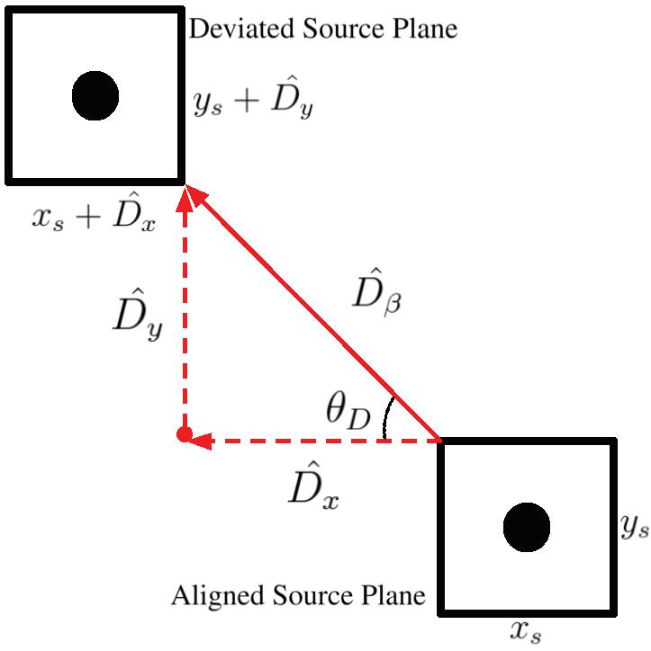
Figure 8. In the figure, we can see that the source is originally aligned with the optical axis. We allow for a source offset from the optical axis by shifting the source plane with a deviance vector D which we can decompose into its components Dx and Dy. With these components, we can transfer every coordinate in the aligned source plane to the deviated source plane by adding Dx and Dy to the x and y coordinates, respectively.

2.4 — Modeling the Source Quasar

To begin testing our lensing model, we must construct an accurate representation for our source. The literature suggests that the source is likely a distant quasar with two extended compact components embedded in a galaxy [10]. Our initial method of modeling assumes a symmetric distribution of matter in the quasar. However this representation resulted in a needless increase in computational load compared to the results of the point source model. We determined that a point source model for the source quasar served as the most effective model.

2.5 — Free Parameters of the Ray Tracing Model

In order to apply our model to MG1131+0456, we must designate free parameters. From previous work by Tonry et al. [6], there is a firm lower bound at redshift z = 1.9 s and an estimated upper bound at redshift z = 5.0. Previs ous findings suggest the source distance as a viable free parameter as it is uncertain and constrained. Additionally, we designate the velocity dispersion of our SIS model as a free parameter. We require the velocity dispersion to be a free parameter because it is one of the largest contributors of both the total mass and mass density, both of which are values we aim to calculate. We have shown through Eq. (7) that the SIS total mass equation requires a radial limit and because of this we allow the radial limit of the lensing SIS to vary within the range of 105 pc to 2x106 pc. We have calculated the angular deviance between the two source components to be θD = 2.8x10−6 radians (Fig. 8).

2.6 — Calculating Variance

Having defined free parameters, before predicting results, we must construct a method to quantify the goodness of fit for our predicted image. We recognize that the source data are pixelated just as our predicted data, but their respective resolutions are not necessarily the same (Fig. 9). We aim to reduce each resolution to a 100x100 image such that we can directly compare individual pixel values to calculate a source variance.

Figure 9. We can reduce a pixelated portion of an image to one individual pixel with a brightness equal to the average of all of the preexisting pixels. In this diagram, we reduce an image with a pixel ratio of 4:1, as apparent because we average the brightness values of a 4x4 square of pixels.

First, we determine the ratio of pixels between the current image and the ideal 100x100 image. For example, if our predicted image was 400x400, we would have a pixel ratio of 4:1 from the predicted to the ideal. Using this, we average every 4x4 square of pixels, which do not overlap, in the predicted image to form one pixel in the reduced image. This process is shown in Figure 9. Additionally, background noise is apparent throughout the image which adds inherent variation when compared to our computational model. To resolve background noise, we apply a lower bound to pixel brightness which filters out noise while retaining the structure of MG1131, shown in Figure 10a.

3. Results

The best fit model for MG1131 using the ray tracing model resulted in a velocity dispersion of 255 km/s,

(a) Reduced Astronomical Data (b) Best Fit Model (c) Overlap Image

Figure 10: (a) Using the methods previously described, we have reduced the radio image of MG1131 to a 100x100 pixelated image where pixel brightness again correlates to percent maximum brightness. This image allows for direct pixel to pixel comparisons between the ray tracing model and the data. (b) Using the ray tracing model we determined the best fit model compared to the reduced and noise-filtered radio imaging of MG1131 using parameters of source distance, velocity dispersion, radial extent of the lensing SIS, and the angular deviance of the source components. (c) By overlapping the best fit image and the observed data of MG1131 we better understand the limitations of the ray tracing model. The observed data for MG1131 are shown in red, the computed image is shown in green, and all overlap is yellow. We are unable to represent the ellipticity that the observed image contains which significantly limits the accuracy of our model. Additionally, the best fit model does include multiple images, but they are not aligned with the multiple images present in MG1131.

a source distance of 3482 Mpc, a β deviance of 2.8x10−6 arcseconds, and a lensing radius of 12500 pc. This simulation was run using a SIS with a radial extent of 25000 pc. Using these parameters and Eq. (7) we calculate a total mass of the lensing galaxy to be 6.98x1011 M sun. Comparing our results to the work of Chen et al. [4] which predicted values in the range of 1.17x1012 M sun to 2.57x1011 M sun, our best fit model is within this range. Our predicted mass using the ray tracing model varied by 46% and 92% compared to the least and most massive models presented by Chen et al. However, compared to the average of the values predicted by Chen et al., 7.14x1011 M sun, there is a percent differnce of 2.2%. The best fit model is shown in Figure 10.

4. Discussion and Future Work

The best fit model using the ray tracing method qualitatively fits the radio image of MG1131 having an Einstein ring and two distinct multiple images of the offset source. However, due to the limitations of the SIS model when applied to an elliptical lens and the assumption of point sources, we cannot represent all features of MG1131 in this model. While the ray tracing model cannot reflect the complex optical strucutre of MG131, our results are within the range of values predicted by Chen et al. [4] which suggest that our model may be able to predict a realistic mass for complex gravitational lenses.

In future work, we aim to further apply the ray tracing model to previously analyzed systems to test its mass predictions against those of the literature. We are first examining the system B2045 +265 shown in Figure 11.

Previous work by Fassnacht et al. concluded that B2045 is "a radio galaxy lensing a radio-loud quasar" [11]. We have shown through the comparing mass predictions for MG1131 with those of Chen et al. [4] that the ray tracing method is viable for modeling strong lensing events by galaxies. The similar structure of B2045 leaves it as an optimal candidate to retest the ray tracing model’s accuracy in mass predictions. Following the literature, we plan to model B2045 with an SIS model and a source represented as multiple point sources [11].

5. Conclusion

The ray tracing model has shown to be a viable method for computationally modeling gravitational lenses but has several limitations at high levels of complexity. We have shown that regardless of these complexity limitations, the ray tracing model predicts a realistic mass model for the gravitational lens MG1131 through comparing our results to the literature [4]. Future work aims to extend the ray tracing model to include a singular isothermal ellipsoid as the mass model to allow for ellipticity in lensed images as well as applying the ray tracing model to B2045 as well as unanalyzed systems.

Figure 11: Images of B2045 from the CASTLeS lensing database and aim to construct a rudimentary model of the system using the ray tracing model. Credit: [7] [11]

6. Acknowledgements

I would like to thank Dr. Jonathan Bennett from The North Carolina School of Science and Mathematics for guidance throughout the research process as well as suggesting the field of gravitational lensing. Additionally, Dr. Bennett’s advice was crucial in designing the ray tracing method. I would also like to thank The North Carolina School of Science and Mathematics and The North Carolina School of Science and Mathematics Foundation for providing me with this opportunity and the funding necessary to produce this work.

7. References

[1] Deceleration Parameter: COSMOS. url: http://astronomy.swin.edu.au/cosmos/D/Deceleration%20Parameter.

[2] Huchra, John P. url: https://www.cfa.harvard.edu/~dfabricant/huchra/hubble/.

[3] Blandford, R. “Cosmological Applications of Gravitational Lensing”. In: Annual Review of Astronomy and Astrophysics 30.1 (Jan. 1992), pp. 311–358. doi: 10.1146/ annurev.astro.30.1.311.

[4] Chen, G. H.; Kochanek, C. S.; and Hewitt, J. N. “The Mass Distribution of the Lens Galaxy in MG 1131+0456”. In: The Astrophysical Journal 447 (July 1995), p. 62. issn: 1538-4357. doi: 10.1086/175857. url: http://dx.doi. org/10.1086/175857.

[5] Hewitt, J. N., et al. “Unusual radio source MG1131 0456: a possible Einstein ring”. In: Nature 333.6173 (1988), pp. 537–540. doi: 10.1038/333537a0.

[6] Tonry, John L. and Kochanek, Christopher S. “Redshifts of the Gravitational Lenses MG 1131+0456 and B1938+666”. In: The Astronomical Journal 119.3 (Mar. 2000), pp. 1078–1082. issn: 0004-6256.doi: 10.1086/301273. url: http://dx.doi.org/10.1086/301273.

[7] C.S. Kochanek, E.E. Falco, C. Impey, J. Lehar, B. McLeod, H.-W. Rix. “CASTLES”.

[8] Freedman, Wendy L., et al. “The Carnegie-Chicago Hubble Program. VIII. An Independent Determination of the Hubble Constant Based on the Tip of the Red Giant Branch”. In: The Astrophysical Journal 882.1 (Aug. 2019), p. 34. issn: 1538-4357. doi: 10.3847/1538- 4357/ab2f73. url: http://dx.doi.org/10.3847/1538-4357/ab2f73.

[9] Congdon, Arthur B. and Keeton, Charles. Principles of Gravitational Lensing. Springer International Publishing, 2018. isbn: 978-3-030-02122-1. doi: 10.1007/978-3-03002122-1.

[10] Kochanek, C. S., et al. “The Infrared Einstein Ring in the Gravitational Lens MG J1131 0456 and the Death of the Dusty Lens Hypothesis”. In: The Astrophysical Journal 535.2 (2000), pp. 692–705. doi: 10.1086/308852.

[11] Fassnacht, C. D., et al. “B2045 265: A New Four-Image Gravitational Lens from CLASS”. In: The Astronomical Journal 117.2 (1999), pp. 658–670. doi: 10.1086/300724.

AN INTERVIEW WITH MR. ERIK TROAN

From left, Jason Li, BSS Editor-In-Chief; Eleanor Xiao, BSS Publication Editor-In-Chief; Dr. Jonathan Bennett, BSS Faculty Advisor; Olivia Fugikawa, BSS Editor-In-Chief; Megan Mou, 2020 BSS Essay Contest Winner; and Mr. Erik Troan '91, founder and CTO of Pendo.io.

To get us started, you are a self-proclaimed technology geek. When was it and what was it that first got you interested in computer programming and engineering?

I’ve been doing [CS and Eng] since I was probably five or six years old. Going back a few decades ago, people didn’t have computers at home, but my father was at IBM so he was always around them. He put me in a programming class at the library when I was probably six or seven. We also had a little computer at school so those two things made me kind of interested in exploring the world. I know what I enjoyed about it then is probably what I still enjoy about it now; it’s a combination of problem solving while doing it in an abstract environment where you really can control a lot of things. Many of you probably enjoy math. Math is fun because there is a right and a wrong, correct? You get to solve a problem. You’re solving a puzzle, but you’re not constrained by inconveniences like physics, gravity, forces, or having to go build things and buy equipment. For me, growing up, it was always a way I could build and explore things. I could do things that didn’t have the constraints of the physical world or have to get materials and put them together. Physical things break and then you have to fix them. So I think that level of control over computer software is really what made me interested in it.

You’ve highlighted NCSSM as one of the most valuable parts of your education. What was your favorite part of your experience there?

The other people. It’s all about the kids. It’s about the social scene—and I don’t necessarily mean social like parties, but social in terms of, you’re in a peer group that’s smart. I’ve probably said something like that at Convocation: you’re not going to sit in a group of people as smart and as energetic and as intellectual and as curious as you are ever again and that leaves a mark. You really do realize there are like-minded people out there; you have interesting conversations and you’re solving interesting problems. I remember I took a fractal class senior year and just the excitement of the kids getting together to solve the problem, and to really learn about it, is what really made an impact on me.

I learned the importance of communication, so I learned to write. I had some very good instructors. I learned from

them that writing was something that helped you communicate, and if you want to become effective in this world, you’re not going to do it mostly one-on-one; you’re going to do it one-to-many. Even in the world of the Internet, Youtube and everything else, writing is probably the most basic way that you’re going to communicate to a lot of people.

I also really fell in love with history, of all things. I had a great U.S. History teacher. That’s followed me my whole life. I’m still a history buff; I read history books all the time. I was so fortunate, just like you, to have instructors who pushed me and made me better all the time. I have a son who is [in NCSSM Online], and it’s great watching him online and how he kicks me out of his room so he can do his classes because he’s getting that extra push and really interesting problem-solving material. He just started his new Bioinformatics class this week and you can just see the lights back on in his eyes.

What do you do at Pendo now? What does a day look like for you?

There are two different parts to that question. My official job at Pendo is that I’m Chief Technology Officer, and that I run all of Product Engineering. All the products that we build come out of my team; it’s a team of about 110 people now. [Our product] runs in the cloud (out on the internet) because it’s a software product. The team deploys that product, keeps it running, manages automated testing, and does 24/7 monitoring. All of that is all under me. So [my job is to] get the product, work with the team that defines what we should build, figure out how to architect it, build it, get it shipped to customers, and keep it up and running.

What do I do every day? I go to meetings pretty much all day—the most important part of my job is helping with communication within my team or across teams. I don’t make the big decisions. If I’m making a decision, there’s probably something wrong. It’s much more about getting the right people in the room, enabling them to make the decision and make sure they feel supported and empowered to make the decision. Asking questions is also a big part of it. I actually sat in your chair a few hours ago going through whether or not we should use a third-party partner for something new we’re rolling out. There was a team of three people that told me two or three weeks ago that they were really excited about it. Now they all changed their mind and all I did was ask them questions about their decision. “Why?” “Have you thought about this?” “What about that?” I didn’t make the decision though. We were going with their recommendation, but I helped to validate and make sure they had the confidence that they thought through everything. So I do that with both Engineering and Product. The other thing I’ll do is work with Sales, Product and Marketing to try to understand the market. I’ll talk to customers about what Pendo does for them and where they are having a problem. I think I have three or four customers that I’m an executive sponsor for, so another part of my job is making sure that they are successful. It’s a lot of talking. I joke that the CTO is actually Chief Talking Officer; some technical in it, but not much.

One thing in a fast-growing organization, you’ll find, is the problems don’t change; the problems change scale. When you solve a problem for a team of 20 with the right solution for 20, when you get to a [team of] 100, that solution probably doesn’t work any more. For example, you might realize that you didn’t have a process for something at 20. That didn’t matter at the time because two people went to lunch once a week, saw each other informally at lunch and communicated, “That’s not working,” or “Fine, I’ll fix it for you.” Then they go back and they fix it. When you get to 100 people, those two people could now sit on different floors and don’t go to lunch any more. All of a sudden, you have a hole where things that were solved informally can’t be solved informally any more because the roles that you need to have around the table drift apart. That doesn’t mean you screwed up, or that your process is wrong, it just means that you’ve grown a lot, and you have to make sure you’re constantly looking for things where you missed or where you can do better. So as you hire specialists, they can thrive without there being gaps between all the specialists.

Do you miss the coding part of your job or the engineering part of your job?

No, because I still do it. This is one of those things where it’s either the best thing about me or the worst thing about me as the CTO. I’m still technical and still want to code. It means I have to hire and surround myself with people who complement that aspect of me. I have two VP’s of Engineering who don’t code. So, I brought people in to take things that gave me a little more room to still be technical. [But] I have to be very careful with what I code. I tend to code things that are longer term, things that aren’t going to be blocking a customer, or things that are not a promise that we are going to get it done by a certain day. I’ve been told that most of the team loves that I [code], because it makes me relatable and I can understand what they’re going through a little more. But it also does mean that there are other parts of my job that I delegate and I do differently because I insist on continuing to code.

What is your advice to students who want to learn more about coding?

Go to school. Go to college. I’m a huge believer in formal computer science education. I hire people who don’t have it, so I do hire coding academies and people who have just

picked it up, but the easy path to success if you want to be in a computer software job is to go to college in computer and software. You will learn things in school that you won’t learn anywhere else. I took a lot of graduate classes as an undergraduate and I still use those lessons. Some of the best engineers have Master’s degrees. I haven’t hired a Master’s degree who’s not a good engineer. These things go together. People get smart in graduate school and undergraduate for a reason, so don’t let that go.

While you’re [in school], do as many internships, real world projects, volunteer projects, and capstone projects as you can. You’ve got to go solve problems. You’ve got to exercise the muscles in your brain to let you try different ways of approaching problems, because there are all sorts of different ways to do it. Unless you’ve done it 20 times, you’re not going to know which [solution] is the best. College and graduate school absolutely accelerate that process.

What is your advice to students who hope to start their own business?

To start a company, you’ve got to find a problem that you are passionate about, not a solution you are passionate about. I tried a [starting a company with a] solution that I really liked and that company fizzled and failed because it wasn’t a problem. Find something you think is worth solving. Find customers who think it’s worth solving—ideally, before you build it. You can’t always do that, but if you can find some way to get people who will validate this as a problem worth paying for, there’s nothing to replace that. One of the reasons I got really attracted to Pendo was, our CEO gave me a problem that I understood, was excited about and resonated with my career. He started talking to potential customers who said, “Oh yeah! Talk to this guy, they said this.” So he could clearly come in with a head start towards, “Was this a valuable problem to solve? What was important about the problem? How is this really going to help customers?”

Another thing I would say is: it is very easy, and I’ve been guilty of this in my career, to take customers for granted. They are going to make you successful. The only things that make you successful are their willingness to pay and your willingness to make them successful. So don’t take them for granted, especially if you’re talking about low prices and products. It’s very easy to say, “Yeah, we have to make it up in volume.” or “If any one customer is unhappy, we can kind of blow it off.” If one customer is unhappy, it’s probably a thousand customers who are unhappy. Make your customers happy. Your customers will carry you everywhere. We have been very lucky here. We’ve done five venture-funding rounds. Every one of them was preempted, so we never went to look for money. Investors came to us, wanting to put money in. The reason that happened was our customers. The first one that found us was because we had already sold to six other portfolio companies, and they started hearing about Pendo, Pendo, Pendo. “What is this thing? Why are you guys all using it?” They were so happy with the value we were delivering that they told their investors about it, who told their partners about it. It happened again and again. It wasn’t any magic. We have seven core values, and one of them is “maniacal focus on the customer.” We are absolutely dedicated to them. I think out of everything I’ve learned, that is the one thing that I have discounted in my career, and I wish I hadn’t. It’s so important.

Many of the students here at NCSSM view failure as something shameful. How did you overcome the failures that you encountered in your life, and how did you learn from them?

Practice. I used to be a private pilot. There’s a saying around that, “The only way to avoid mistakes is through experience, and the only way to get experience is by making mistakes.” Failure is a side effect of taking a chance, taking a risk, pushing your zone. If you don’t fail, you’re not trying very hard. And I get it—I watched my kids go through middle school and high school. I get that we built a society for students where failure can be very, very expensive. You guys get that one “C” in a class, and there’s colleges you might not get into or scholarships you might not get. You’re in a weird place in high school. Don’t mistake how you succeed in that microcosm for how you’re going to be successful in life. You’re going to be successful in life by growing, learning, and trying new things. One of the reasons that [the US] is still one of the premiere economies in the world is that we don’t punish failure. I failed in my last company. It was a big crater in the ground, burned through tens of millions of dollars of other people’s money. When I helped raise money for Pendo, people saw that as a plus. They didn’t say, “Well, your last one failed, why would I invest in you now?” They said, “Hey, what’d you learn?” and I said “This and this and this, oh my god I learned so much,” and they’d say, “Great, let’s do this.” You’re lucky to be in a country that, as you move out of that narrow, high-achieving academic track that you’re on, failure won’t always be punished. So embrace it and try things. You have to try new things or you won’t get better. I have a really smart PhD [employee] here, who worked on a project for 6 months. He spent 6 months of engineering on something. It didn’t work. At the end of the day, we had to shelve it. But if we didn’t try, we would always be wondering “What if?” We had to figure out other ways to solve it, and that approach was a bad one. So, I get why kids at Science and Math and in high school are scared of failure; I think you’ve been taught your whole lives to be scared of failure. Just try and get over it when you’re in college. It’s going to be very hard to do anything special unless

you take some gambles. You can’t win every gamble. But when you fail, look at why. I learned more from the company that didn’t work than from the companies that did. I’ve hired people who have been fired, by the way. The question is, “What did you learn from your failure? Why did it not work? What was it about you that had to change?” and if they say “it was the company, there were bad people there, they didn’t listen to my ideas, they did everything I told them not to” — run away. That’s not learning. If they say “Yeah, the company had this culture, and I brought this culture, and I had trouble adapting,” or, “I really thought this was gonna work out, and I pushed hard for it. I think I alienated some people” — those are the kind of people you want, because they’ll probably be better next time.

What do you enjoy doing outside of work?

I scuba dive. I’m actually a scuba instructor, so I teach one or two classes a year. I’d like to get back into flying; I’m looking into doing that in the next year or two. I’m a pretty avid snowskier; I try and go out west a couple times a year. I run hundreds of miles a year—that’s not something I enjoy, I do it because I’m old. I like to cook. It’s the highlight whenever we can get the whole family around the table. I have 3 teenage boys, so it doesn’t happen that often, but when we can all sit down to a meal, our meals tend to last one and a half, two hours. They’re very long, drawn-out meals after the food’s all gone. We don’t see each other that much so we enjoy that. I like to travel. Whenever I can, I’ll take a trip overseas—not for work, but if I can travel personally, it’s great to just be in a new place and wake up somewhere else. I also like to read. I read a ton.

As a scientist who works in the entrepreneurial side of things, what do you have to say about the role of entrepreneurship in advancing science?

First of all, I’m not a scientist, I’m an engineer. I consider those really, really different. When I didn’t go to grad school, I turned away from being a scientist. Scientists discover new things. Engineers try and apply science to problems. I think engineering and entrepreneurship are really tightly coupled. My personal belief is that most of the time if you engineer something new, you probably need a new company to really make it successful. The iPhone is a huge counterexample to that, but most truly novel engineering projects have a company to go off of because [they’re] bringing something new to the market.

Science is harder. A lot of science has around 30 or 40 year payback periods, and it’s not that they’re not interesting topics and that they’re not important. If you’re lucky enough to be a scientist, and you’re able to do it in an entrepreneurial sense, I think that’s great. But for most science, I think, you need to figure out how to do it through research grants and universities where you don’t need to have that immediate payback period.

Some of the most interesting things that come out of science start as an intellectual curiosity. They didn’t start off as solving a real-world problem, but they all feed into real-world problems, into the hands of people like me, who are engineers. When you start crossing those wires too much, you get into bad positions like you have in medicine, where a lot of research in medicine is being privatized. If it isn’t for a disease that has enough payback, then it gets shelved, so you start getting the wrong incentives around basic research.

How important is entrepreneurship for applying the knowledge that comes out of science, or for doing engineering?

I think for building real solutions to real problems, it’s critical. If all we had in the world was fifty Fortune 50 companies, then we wouldn’t get innovation, and we wouldn’t get new products to solve new problems out there. The easiest example is alternate energy. It’s not Exxon and BP that are bringing alternate energy and clean energy to the world. They have a business—they dig up oil, refine it, burn it, and make a lot of money doing it. It’s hard to take a business like that and go do something that’s new and different. It’s a risk. It’s a lot easier to take a risk as an entrepreneur because you have a lot to gain, but if you’re running a big company, how do you value that risk? You have a lot to lose.

[Entrepreneurship] is critical. I think universities are normally pretty bad at it. Stanford is uniquely good at it, and I don’t know if it’s [because they’re] Stanford or if it’s because they’re sitting in the middle of Silicon Valley and have hundreds of billions of investment capital sniffing around looking for the next opportunity all the time. Mostly it’s disappointing when you look at universities that have so much pressure to raise money and own part of their inventions that they aren’t good at getting these companies up or bringing the technology up. Which is too bad because I think there’s a huge amount of symbiosis between those two.