The North Carolina School of Science and Mathematics – Durham Journal of Student STEM Research
Front Cover
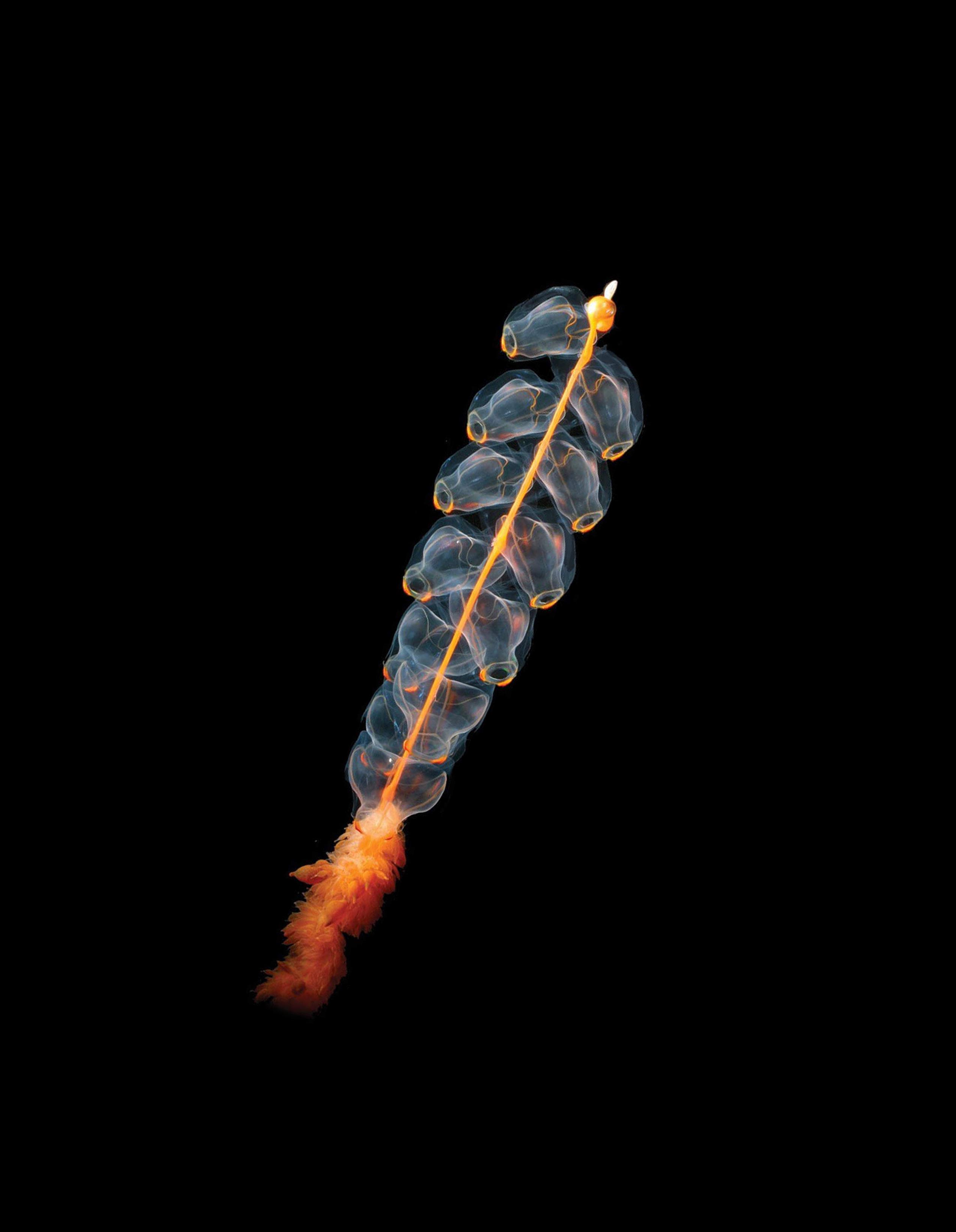
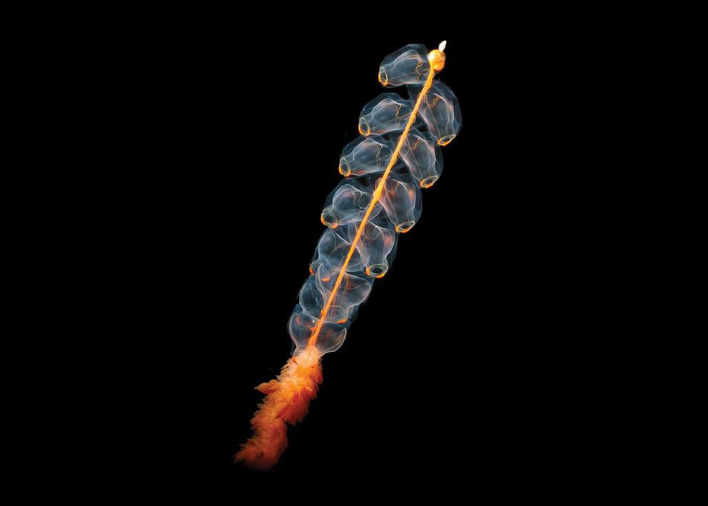
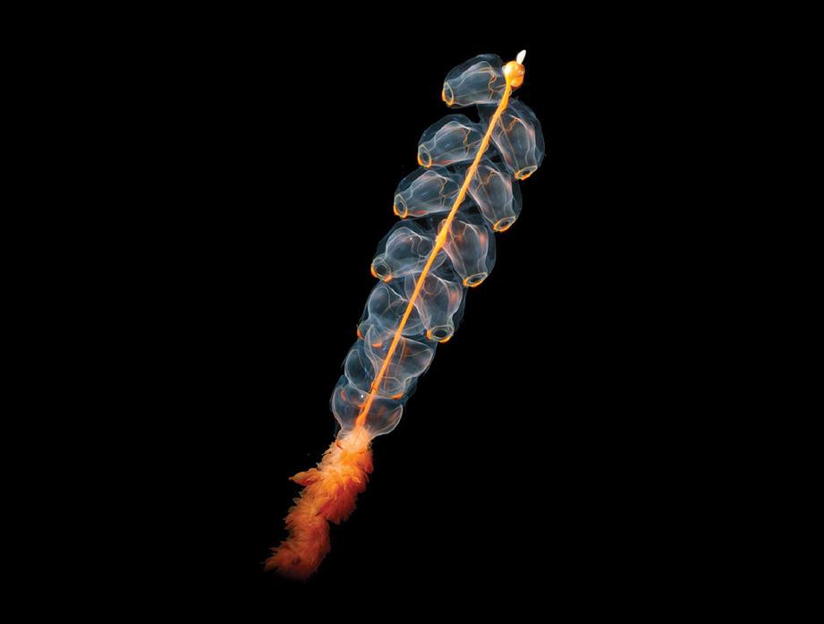
Marrus orthocanna is a deep-sea siphonophore more alien than earthly. Orthocanna is composed of many individual organisms that work to function as one. These zooids, shimmering on orthocanna's blazing orange nectosome, showcase how evolution can sculpt forms as otherworldly as anything imagined beyond our planet.
Credit: Kevin Raskoff, California State University
Biology Section
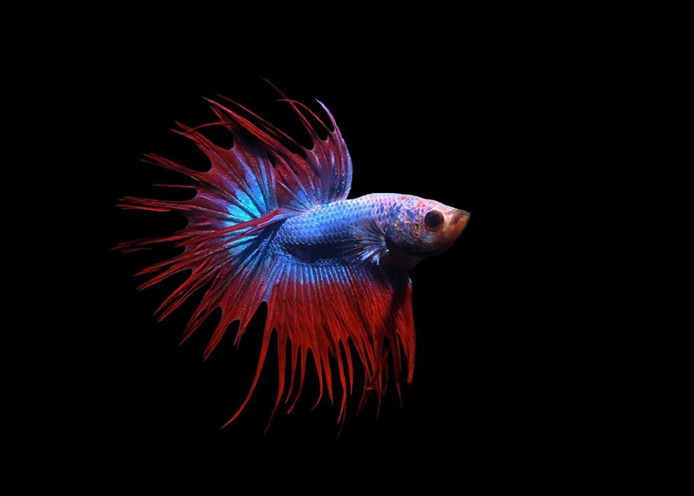
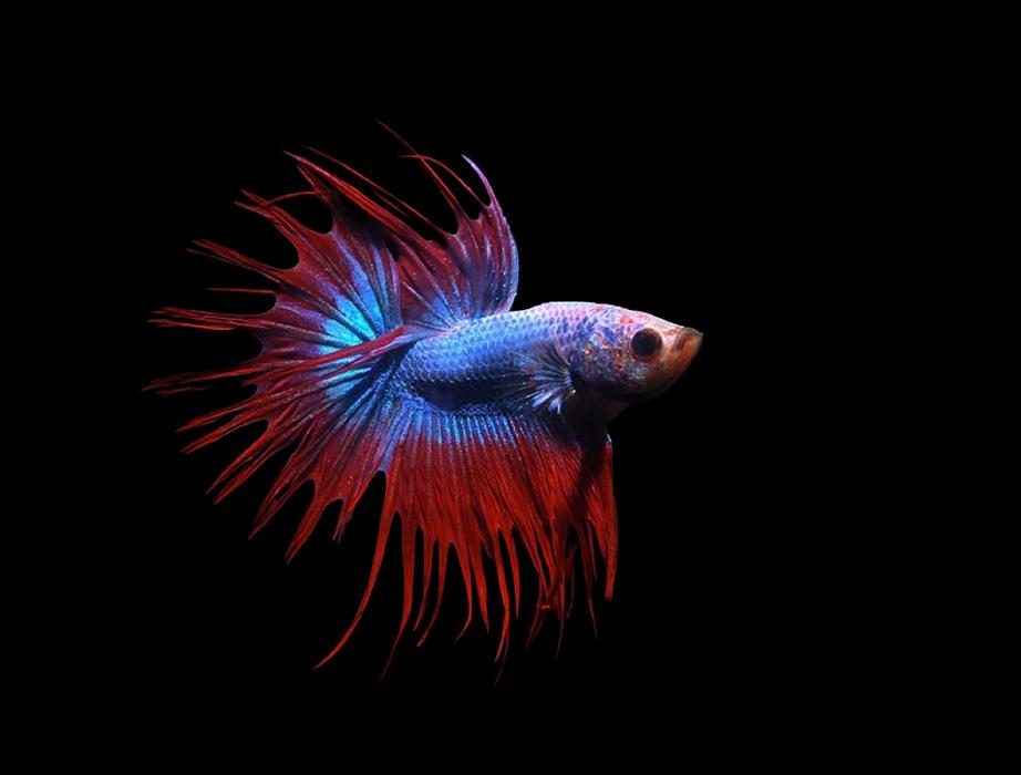
The image shows a male siamese fighting fish (Betta splendens) with a striking crowntail fin type, featuring long, spiky, and dramatically fringed fins that resemble a crown. Its vibrant colors and elaborate fin structure highlight its aggressive yet captivating beauty.
Credit: Anandarajkumar, used under terms of the GNU Free Documentation License
Chemistry Section
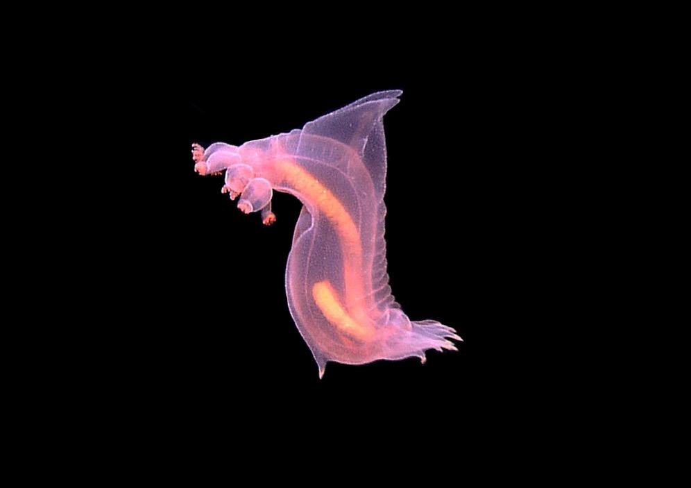
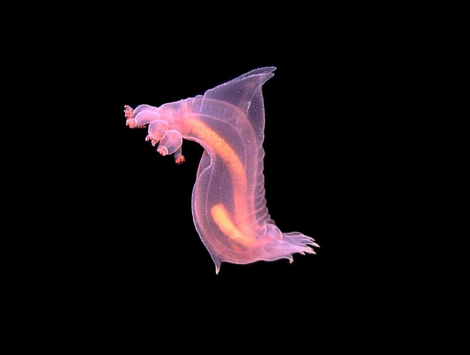
The image shows Enypniastes eximia, also known as the headless chicken fish, a deep-sea sea cucumber with a translucent, gelatinous body. It has fin-like appendages that allow it to swim gracefully through the water column above the ocean floor.
Credit: Creative Commons License
Engineering Section
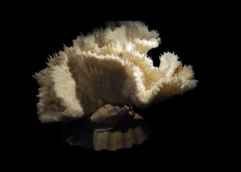
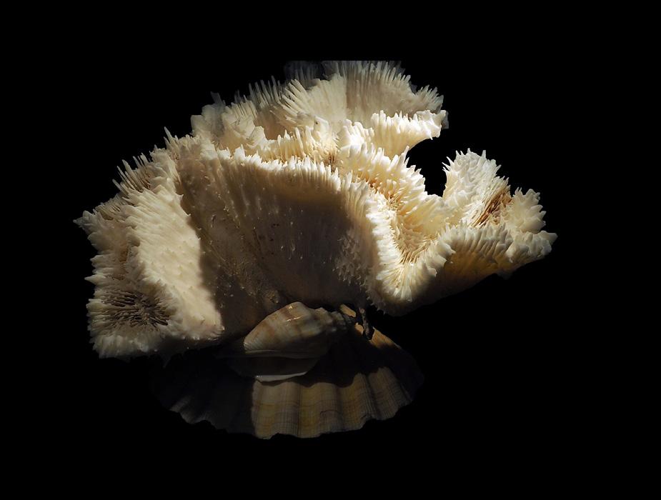
This image shows an unidentified coral sample from the Indian Ocean. It is currently in the colection of the Cantonal Museum of Geology in Lausanne, Switzerland.
Credit: (C) adafruit.com used with permission
Mathematics and Computer Science Section
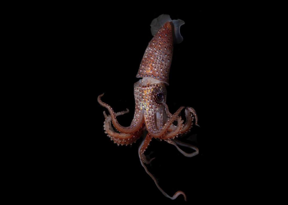
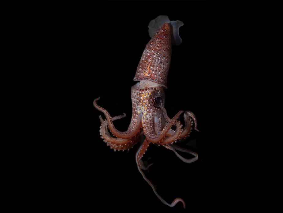
The image shows a very large strawberry squid (Histioteuthis), notable for its reddish, speckled body that resembles a strawberry. One of its most striking features is its mismatched eyes, one large and one small, adapted for detecting light in the deep sea.
Credit: National Oceanic and Atmospheric Administration Fisheries
Physics Section
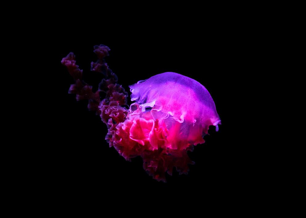
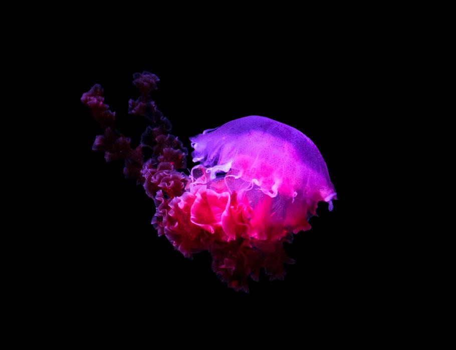
The image shows Pelagia noctiluca, a luminous jellyfish known for its glowing, pinkishpurple bell and long, trailing tentacles. Commonly called the mauve stinger, it’s often seen drifting through open oceans, emitting bioluminescent flashes when disturbed.
Credit: Matt Alaniz, under Unsplash License
11
SAJAN PATEL, 2026
BEN SHEEGOG, 2026 ONLINE
VINCENT SHEN, 2025
CHARLOTTE GOEBEL, 2025
Cloning the Anhydrobiosis Protein CAHS-89226 from Hypsibius exemplaris to Construct Desiccation-Tolerant Azotobacter vinelandii and Escherichia coli
ARETHA DATTA, 2025
24 Effects of Hypercholesterolemia and the Inhibition of AGE-RAGE Pathway on Exopher Formation in C. elegans
ANNELIESE HEYDER, 2025
31 Enhancing the Efficacy of Riparian Buffer Zones Using Native Grasses and Symbiotic Fungi in Relation to Overflowing Hog Waste in Rural North Carolina
SKYLER QU, 2025
44 Menthol Modified Carbon Dot Based Vesicle Nanoparticles with Enhanced Blood Barrier Penetration and Tumor Targeting Ability
VINCENT BARBORIAK, 2025
52 The Development, Synthesis, and Testing of Low-Spin Mn(I)-Centered Catalysts to Aid in Chemical Recycling of Plastic Waste
DYLAN DEES, 2025
59 Design, Synthesis, and Testing of Novel Inhibitor-Based Pharmacological Chaperones for Tay-Sachs Disease
LEAH NIKHIL, 2025
Engineering
68 Assessing the Mechanical Properties and Morphology of Biomimetic Nanofiber Hydrogel Composites for Articular Cartilage Scaffolds
ARIANNA LEE, 2025
Mathematics and Computer Science
77 Improving Robotic Arm Precision and Accuracy Using a Novel Quantum Kolmogorov- Arnold Network Algorithm
SPENCER HIRSCH, 2026 ONLINE
87 "Can You Even?" An Exploration of Polyominos
PEYTON JACKSON 2025, TATIANA MEDVED 2025, MATIAS RELYEA 2025
95 Unified Deep Learning and Machine Learning Ensembles for Robust Depression Detection
RICHARD SHAN, 2026
Physics
107 Analytically Modeling the Gravitational Radiation Generated from a Quasistar System
JEREMY ADAM, 2025
115 Investigating the Morphologies of Local-Scale Dust Storms in the Northern Hemisphere of Mars
JOHNATHAN STRICKLAND, 2025
Featured Article
125 An Interview with Dr. Daphne Klotsa
LETTER from the CHANCELLOR
“The
good thing about science is that it’s true whether or not you believe in it”
Neil deGrasse Tyson
I am proud to introduce the fourteenth edition of the North Carolina School of Science and Mathematics’ (NCSSM) Durham campus scientific journal, Broad Street Scientific. Each year students at NCSSM-Durham conduct significant scientific research, and Broad Street Scientific is a student-led and student-produced showcase of some of the impressive research being done by students on our Durham campus.
Opened in 1980, NCSSM was the nation’s first public residential high school where students study a specialized curriculum emphasizing science and mathematics. Teaching students to do research and providing them with opportunities to conduct high-level research in biology, chemistry, physics, computational science, engineering and computer science, mathematics, humanities, and the social sciences is a critical component of NCSSM’s mission to educate academically talented students to become state, national, and global leaders in science, technology, engineering, and mathematics. Today, nearly 90% of NCSSM students conduct research during their two years at NCSSM. I am grateful for our talented NCSSM faculty and mentors at institutions across
our state who provide these incredible opportunities for students, on two campuses and in our online program, to learn research methods and conduct high quality research. I am proud that at NCSSM, we strongly support developing the next generation of scientists and researchers who will use science to help develop new technologies and solve our most challenging problems for many years to come. Amazing things happen when you bring talented student researchers together with incredible faculty and I am excited that this year’s publication of Broad Street Scientific provides another opportunity to share with the broader community the outstanding research being conducted by NCSSM students.
I would like to thank all of the students and faculty involved in producing Broad Street Scientific, particularly faculty sponsors Dr. Jonathan Bennett and Dr. Michael Falvo and senior editors Advika Arun, Ankit Biswas, Joshua Chilukuri, John Guo, Adrian Tejada, and Nikhil Vemuri. Explore and enjoy!
Todd Roberts
Dr.
Chancellor
WORDS from the EDITORS
Hello and welcome to the Broad Street Scientific, NCSSM Durham’s official journal of student research in science, technology, engineering, and mathematics! Now in its second decade of publication, the Broad Street Scientific continues to evolve and thrive as a journal. This past year we have expanded enrollment in our JTerm course offering, providing a structured introduction to scientific writing and research to a record number of NCSSM students.
These changes have allowed Broad Street Scientific to more fully meet its underlying mission: highlighting and celebrating the excellence and breadth of student research at NCSSM. This year’s edition of the Broad Street Scientific does just that. From explorations into the theoretical physics of quasistars to the development of novel methods for plastic recycling, the student research presented in this edition pushes the boundary of science and innovation.
This exploration of the seemingly familiar is celebrated in the journal’s theme this year: the deep sea. The deep sea is where life began, nurtured by nutrientrich hydrothermal vents thousands of feet below the ocean’s surface. From humble beginnings and simple chemical reactions, the organisms that call the deep sea home gave rise to a vast tree of life that expanded to the land, air, and sea. And yet, the deep sea remains one of humanity's most unexplored frontiers, more alien to us than the surface of Mars.
This past year has been one of great growth and improvement for the journal. It has expanded its efforts to educate on scientific writing and editing, welcoming more students than ever to its annual, 2-week JTerm class. As the journal continues to move through its second decade of publication, it has also remained truer than ever to its goal of celebrating the excellence and breadth of student research at NCSSM. These improvements in our 14th edition allow us to continue showcasing exceptional research, innovative ideas, and collaboration within the students of North Carolina School of Science and Mathematics.
We would like to thank the faculty, staff, and administration of NCSSM, particularly Chancellor Dr. Todd Roberts, Dean of Science Dr. Amy Sheck, and Director of Mentorship and Research for the Durham campus Dr. Sarah Shoemaker. They continue to support and nurture a stimulating academic environment that encourages motivated students to apply their interests towards solving real-world problems. For the next generation of young people who will no doubt change the world, NCSSM serves as a nurturing environment of passion and determination. We also extend special thanks to Dr. Jonathan Bennett and Dr. Michael Falvo for their invaluable support and guidance throughout the publication process. Lastly, we would like to acknowledge Dr. Daphne Klotsa for a fascinating conversation on active matter.
Advika Arun, Ankit Biswas, Joshua Chilukuri, John Guo, Adrian Tejada, and Nikhil Vemuri
Editors-in-Chief
BROAD STREET SCIENTIFIC STAFF
Editors-in-Chief
Advika Arun, 2025
Adrian Tejada, 2025
Nikhil Vemuri, 2025
Publication Editors
John Guo, 2026
Sneha Khetan, 2026
Sindhu Paladugu, 2025
Zoey Zhang, 2026
Biology Editors
Jiah Lee, 2025
Adarsh Magesh, 2025
Grace Pan, 2026
Chemistry Editors
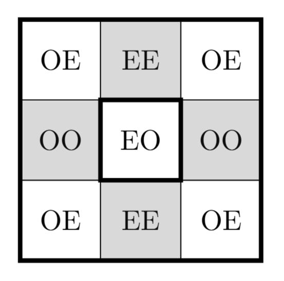
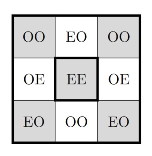
Pragathi Akula, 2026
Chloe Harnphanich, 2026
Vishnu Vanapalli, 2025
Engineering Editors
Sanika Agarkar, 2026
Sarah Zhou, 2026
Mathematics and Computer Science Editors
Physics Editors
Joshua Chilukuri, 2026
Tanuj Karthikeyan, 2026
Ankit Biswas, 2026
Jahnavi Bondada, 2026
Faculty Advisors
Dr. Jonathan Bennett
Dr. Michael Falvo
LIT FROM WITHIN
Nandhini Thangamani
Nandhini Thangamani was selected as the winner of the 2025 Broad Street Scientific Essay Contest. Her award included the opportunity to interview Dr. Daphne Klotsa, Associate Professor in Applied Physical Science at the University of North Carolina at Chapel Hill.
“We are stardust brought to life, then empowered by the universe to figure itself out…”
Pick a leaf off a tree and trace its edges; notice how the thin lines branch from the center stem. Look up at the tree, and study how the tree’s branches bloom from the trunk in the same way. Peripheral nerves spanning your body branch out from the spinal cord just like the tree. Your ear’s curve follows the same mathematical pattern as the swirls of a conch shell, the Fibonacci sequence hidden in plain sight. The whorls of your fingerprints are reminiscent of the grooves of a ram’s horns, a tug of war between phenotypes and genotypes. Eight possible patterns at the tips of your fingers: radial, ulnar, double, central pocket, arch, tented arch, whorl, and accidental. Combinations are practically limitless, infinite possibilities right at your fingertips, comparable to the number of stars in the sky.
The elements forged in the hearts of stars: nitrogen, carbon, hydrogen. Stars, composed of the hydrogen that runs through your veins.
"Are we made of stardust or are the stars made of us?"
We see the stars as beautiful extraterrestrial creations far away from our humble Earth, even though we might be made of the same elements. If stardust truly runs through the veins of the Earth and within every living being, shouldn’t we regard Earth with the same reverence as we do the stars?
To figure out whether we are made of stardust, we first have to find the chemical makeup for each star. We look at starlight through a prism and its absorption spectrum, showing a unique fingerprint for every element in the star. We thought we had an answer then, that their makeups would vary as widely as math can compute. But Cecilia Payne discovered that stars are mostly hydrogen, a little helium, and almost nothing else– “No, this can’t be right.”
“Are we different from everything that surrounds us?”
Looking through the center of nebulas, huge clouds of dust and gas, lit from within like a nightlight by nearby stars, we found the same hydrogen and helium. Stars are so similar to each other, but not to Earth, forming an extraterrestrial community we cannot dream of joining. So, we learn and we theorize and we research.
We look up at the stars for answers, but they just twinkle silently, shining with laughter.
"Maybe our answers will be closer than we thought."
"Maybe, we are the universe studying itself."
Biology echoes and ripples, repeating its own history. Thousands of years of evolution within the theropod lineage led to the sharp look in a rooster’s eyes as it watches the sunrise, the same as the Tyrannosaurus rex as it hunted down its prey.
Physics sings through your fingers as you hold your hand up to the sun, particles of light scattering as you glow orange from within. An entire world of subatomic particles, so small they go unobserved, yet they form our entire world and all of us in it. Electrons play, jumping from energy states like children on the playground, releasing photons with wavelengths of visible light, painting our world.
Mathematics translates these wavelength patterns into a way we understand. It's the language of the universe, taking those waves and describing them through Fourier transfers, as a sequence of sine and cosine functions. It makes the world tangible to our human minds. Disease spreads like wildfire through populations and differential equations trace its origin through finding the rate of change of the infected.
We have always sought to chart these patterns, the desire to understand the world around us transcending generations. Hipparchus, an ancient astronomer, craned his neck up at the sky and cataloged more than 850 stars by hand, painting constellations of unicorns and dragons. We seek meaning beyond what is confined by Earth when we create meaning with every bit of research we conduct.
Research and innovation is driven by our innate curiosity and sense of wonder. Every invention on Earth is made from love. A surgeon created medical latex gloves for his wife who would come home from her nursing shifts with irritated hands. To let his wife enjoy baked goods even though she was allergic to yeast, a chemist formulated baking soda. The original Band-aids were invented by a man who wanted to prevent his wife’s small cuts on her fingers while cooking.
The very first sign of civilization was a healed femur. A broken thigh bone several hundred years ago was a mark
of death, leaving one unable to run from predators or forage for food. Unless they were taken care of for several months, even though they could not contribute to the tribe. They were fed, dressed, protected, and warmed by love.
William Shatner ventured to space, yearning for meaning greater than what is weighed down by Earth’s gravity. He spent his life popularizing the idea that space is the final frontier on the show Star Trek. But when he actually reached this magical destination, floating through black infinity, he turned back to look at us. He saw the blue curve of the atmosphere, ridges of beige and green, white clouds swirling and shifting. So far from humanity, he realised everything worth marveling at is already on Earth.
The smile lines carved into your face like rivers meandering through the land and the delicate mole hidden under your collarbone are unique and special to only you. What you are made of is the same as everyone and everything around you, yet nothing can compare to what is in you. The secrets that you hide in your dreams, wishes blown away on dandelions, and pinky promises made in the corners of your hometown carve out your spot in the universe.
This coincidence that brought us here together– it’s not insignificant and shouldn’t be brushed over. Sit by the ocean and breathe, let the waves send wavelengths to your ears and hear the thrumming chorale of millions of drops of water. Do they sound like discordant crashes, or the steady beat of a strong heart?
Stare at the ocean during nighttime, dangling your legs above its surface and watching it come alive. A black void, mirroring the sky above. A sea full of stars blinking back at you.
We’ve mapped less of the seafloor than we have of the surface of Mars. A pool full of mysteries beneath our feet, yet few dare to venture into its depths.
Octopi potentially dream. If so, these invertebrates have developed a two-cycle sleep similar to vertebrates completely independently, with millions of years of evolution between them. During states of high rapid eye movement (REM) sleep, we dream the most. Yet no one knows why we dream. Whether it is our brain’s subconscious coming to the forefront, routine cleansing of the memory, or another theory, we constantly dream of new ideas for this mystery. Meanwhile, the little octopus slumbers, unbothered.
Dive deeper into the ocean and find almost alien life, not foreign to Earth but foreign to our preconceived notions of what life on Earth resembles. The first fish that crawled on land marked the fork of evolution; one side with land adaptations and the other with aquatic adaptations. With little to no light and a full range of movement unconstrained by gravity, ocean
life has evolved unpredictably. The Barreleye Fish with a transparent head so its huge green eyes, built like barrels, can look up, but also swivel to face forward. The Mystery Mollusc–initially confused to be a sea snail, hence the name–uses its hood in a similar fashion to a Venus Fly Trap plant to ensnare prey. More than 91% of ocean creatures have yet to be discovered, unlike anything we’ve thought possible on Earth. Perhaps the jaw-dropping life we’ve assumed only exists on a distant planet roams the very same Earth as us.
Our own Earth, unlike any other we know, ravaged by climate change and rising carbon emissions, still has so many wonders to discover. Looking around with the eyes of a scientist, itching to understand, can change your perspective of the world, and thus, eventually change the world itself. Geologists find pleasure in a pile of rocks and ornithologists spend hours bird-watching. Love and passion for the sciences drives us to the point of invention, continuously building upon generations of discoveries to add more research and benefit humanity. The stars live and die in brilliant supernovas, but their light travels on, illuminating the universe for years to come.
Us, made of stardust on a planet unlike any star. The odd one out in the known universe.
Alien.
Marvel at Earth’s wonders as if they were extraordinary. For the extraterrestrial is already here.
“…and we have only just begun.”
- Neil deGrasse Tyson
PHOTOGRAPHY:
Sajan Patel, Ben Sheegog, Vincent Shen, and Charlotte Goebel
Sajan Patel, Ben Sheegog, Vincent Shen, and Charlotte Goebel were selected as the winners of the 2025 Broad Street Scientific Photo Contest. Their awards included the opportunity to have their photographs featured in the 2025 volume of the Broad Street Scientific.
The Silent Guardians of the Patagonian Coast by Sajan Patel
Pictured are two Magellanic penguins standing in the fairly desolate landscape of Isla Martillo, located in the coastal Tierra del Fuego of Patagonia. Rugged terrain, sparse vegetation, and barren trees silhouette against a brooding sky. As a near-threatened species, their conservation must be prioritized to maintain Argentina’s natural biodiversity.
The Waking City by Ben Sheegog
This image captures a city waking beneath a blanket of fog as its skyline emerges in soft golden hues. The muted lights hint at lives awakening below, and the mountainous backdrop reminds us of where their roots are planted.
The wilderness of Alaska’s interior includes the New Hampshire-sized Denali National Park, which boasts North America's tallest peak. This photograph was captured from inside an airplane in late May, with the summer season seeing 16-19 hours of sunlight a day.
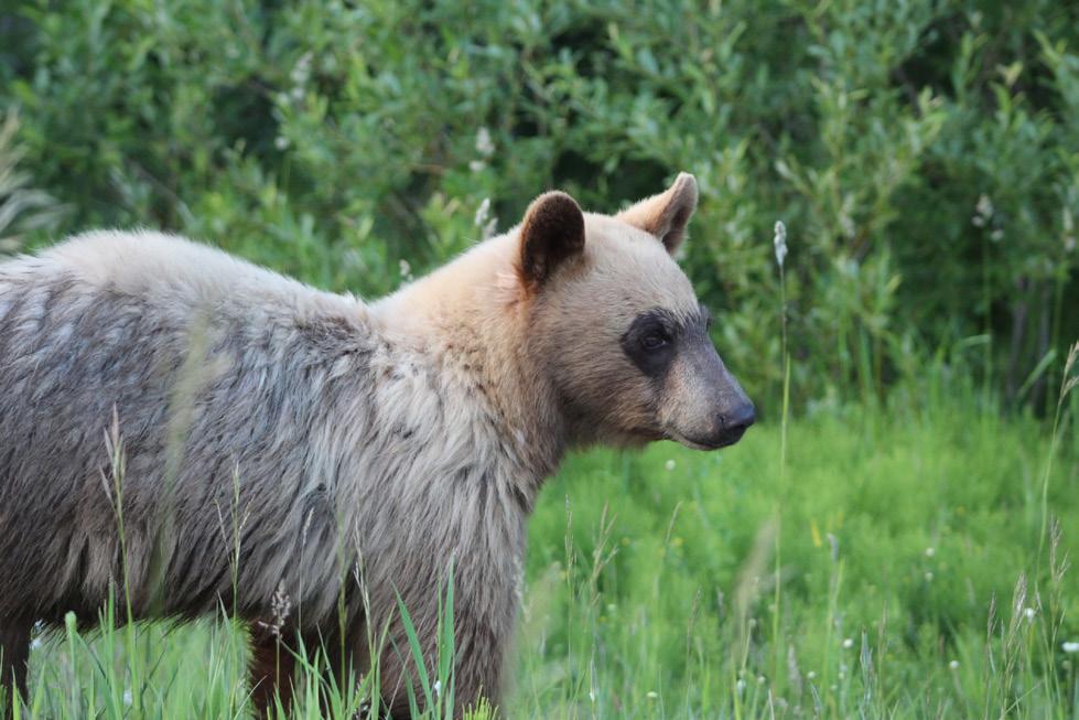
This blonde bear grazing in Glacier National Park, Montana, is an American black bear, disinguishable by its tall ears. It seems to smile in the fading summer light, enjoying the Park's serenity.
Interior Alaska by Vincent Shen
Glacier Brown Bear by Charlotte Goebel
CLONING THE ANHYDROBIOSIS PROTEIN CAHS-89226 FROM HYPSIBIUS EXEMPLARIS TO CONSTRUCT
DESICCATION-TOLERANT AZOTOBACTER VINELANDII AND ESCHERICHIA COLI
Aretha Datta
Abstract
Many rare diseases remain uncured, resulting in numerous global deaths annually. While cryopreservation—a way to pause aging through freezing—has been successful in animals, it has yet to be effectively applied to humans. Additionally, with the commercialization of space travel and NASA’s initiatives to colonize Mars and the Moon for resources, space travel and interplanetary colonization sectors have begun to grow, requiring enhanced spacecrafts for prolonged space travel. However, current space travel methods present significant challenges, including detrimental health effects and high resource costs, making long-term missions unfeasible. To address these challenges, mechanisms similar to anhydrobiosis, or desiccation, as observed in tardigrades like Hypsibius exemplaris, should be explored. This study aims to clone the CAHS-89226 gene—which is believed to play a role in desiccation tolerance in H. exemplaris and insert it into Azotobacter vinelandii, a bacteria known for using cysts as a method of tolerating desiccation, and Escherichia coli, a bacteria known for its relatively low desiccation tolerance. Although H. exemplaris is readily available in laboratory settings, its genome remains incompletely sequenced, making the confirmation of CAHS-89226 an important finding. The successful extraction of CAHS-89226 with sticky ends paves the way for future recombinant plasmid design. Importantly, this study reveals no significant loss in cell viability following electroporation and heat-shock transformations for A. vinelandii, but the opposite for E. coli. This research lays the groundwork for future investigations into the relationship of CAHS-89226 with other stress response genes. Ultimately, mechanisms of desiccation may provide a more economically viable and practical alternative to cryopreservation, potentially facilitating advancements in space travel and improving survival prospects for humanity.
1. Introduction
1.1 Space Travel
As space travel becomes increasingly commercialized and no longer solely government-controlled, the colonization of other planets emerges as a common question. Upcoming missions to Mars and the Moon are paving the way for the broader human expansion into space (Moon to Mars Architecture - NASA, 2024). In the future, such colonization may occur on distant planets suitable for human settlement. For example, NASA’s Kepler mission discovered a larger, older Earthlike planet called Kepler-452b about 1,400 light years away (Jenkins et al., 2015). With current spacecraft and aviation technology, the expected travel time to Kepler452b is 26 million years (Creighton, 2017). For this level of space travel, intergenerational travel would be necessary, posing multiple risks, including a large resource expense,
spaceflight-borne chronic and infectious illnesses, and negative psychological effects (Yin et al., 2023). Moreover, various risks are associated with spaceflight, such as circadian rhythm dysregulation (Yin et al., 2023), early onset cell senescence (Garbacki et al., 2023), muscle and bone degradation (Man et al., 2022), loss of vision or hearing (Buckey et al., 2018), reduced immune function (Lv et al., 2023), and mitochondrial dysfunction (Waisberg et al., 2024).
To mitigate these risks, scientists are exploring cryptobiotic capabilities—the ability to pause biological functions under extreme conditions—to preserve human health during transit. This approach would allow travelers to enter a dormant state, potentially pausing the aging process and reducing resource needs for essentials like fuel, food, and water. The reduced human activity aboard the vessel would also help minimize health risks during the journey.
1.2 Cryonics
Over 6,500 rare diseases currently lack a cure, and when more common diseases are considered, the number of untreatable conditions is significant (Rare Diseases, 2020). Such diseases, like rabies, are fatal, and often lead to excruciatingly painful deaths, highlighting the need for solutions beyond current medical technology. Cryonics, the practice of freezing recently deceased individuals in hopes of future revival, offers one potential pathway to overcome the limitations of today’s medicine. Despite successful cryopreservation in animals, humans have yet to be successfully cryopreserved (Ekpo et al., 2022). Since human cryopreservation remains unachievable, studying organisms like tardigrades, which can enter a state of cryptobiosis, could offer promising insights. Cryptobiotic capabilities in tardigrades might one day be adapted for human applications, potentially allowing the safe preservation of human tissues—or even whole bodies—until medical advancements are available.
1.3 Hypsibius exemplaris
Tardigrades are an extremotolerant species (Yoshida et al., 2021; Joseph, 2023), meaning they can survive the harshest environments in the world, including outer space (Møbjerg & Neves, 2021). Since tardigrades are limnoterrestrial, or only active when covered by a thin film of water, they are not well equipped to survive dry climates. Thus, when tardigrades are exposed to an arid environment, they enter cryptobiosis, more commonly known as a “tun state”, and do not exit it until they have enough water exposure (Møbjerg & Neves, 2021). In this state, they reduce body volume by 85-90% (Møbjerg & Neves, 2021), retaining only 2-3% of their extracellular and intra-cellular water content (Møbjerg & Neves, 2021). Tardigrades have five different forms of cryptobiosis they use to survive: anhydrobiosis (desiccation), osmobiosis (rise in external pressure), cryobiosis (freezing), anoxybiosis (lack of oxygen), and chemobiosis (exposure to environmental toxicants) (Møbjerg & Neves, 2021; Wełnicz et al., 2011; Roszkowska et al., 2021; Lim et al., 2024; Hibshman et al., 2020). In this state, they do not biologically age (Kasianchuk et al., 2023; Sieger et al., 2022), allowing them to be well-suited for long-term travel. The 1,300 different species of tardigrades on planet Earth have varying levels of anhydrobiosis capabilities (Tardigrade). Many of these anhydrobiotic capabilities are believed to be due to three main proteins: CAHS (Cytoplasm-Abundant Heat Soluble), SAHS (SecretoryAbundant Heat Soluble), and MAHS (MitochondrialAbundant Heat Soluble) (Kasianchuk et al., 2023; Boothby et al., 2017).
Hypsibius exemplaris is an herbivorous species of tardigrade commonly used for evolutionary biology and astrobiology research due to its anhydrobiotic capabilities (Poprawa et al., 2022; Gąsiorek et al., 2018). However, currently, only fractions of H. exemplaris’s genome have been sequenced and annotated. As Ramazzottius varieornatus was fully sequenced by Takekazu Kuneida, it was proposed as a suitable alternative. However, due to its unavailability in North Carolina and the challenges of rearing it, the next most accessible tardigrade, H. exemplaris, which is easy to rear and maintain, was selected instead (Hashimoto et al., 2016).
1.4 CAHS-89226
CAHS (Cytoplasm-Abundant Heat Soluble) is a TDP (tardigrade-intrinsically disordered protein) and is thought to be used in tardigrades to protect and preserve cellular components through desiccation (Barilla et al., 2024). CAHS is believed to produce a “bioglass” out of the cytoplasm, effectively suspending the cell in a certain position, thus stopping all metabolic processes, as no part of the cell moves or reacts (Barilla et al., 2024). In Hypsibius exemplaris, the CAHS-89226 gene is proposed to exist, though not confirmed, as the entire genome has not been sequenced (Hypsibius Exemplaris Genome Assembly nHd_3.1, n.d.). Additionally, the relationship between CAHS-D and trehalose, a sugar used for long-term cell desiccation (Tapia et al., 2015), is synergetic. Trehalose is not synergistic with numerous other desiccationresistant proteins, like Bovine Serum Albumin (Nguyen et al., 2022). This tells us that CAHS plays a role in desiccation tolerance, as trehalose alongside CAHS had a greater survival rate than either factor alone. Thus, many scientists believe that CAHS plays a role in the superior desiccation tolerance of tardigrades. Understanding the role of CAHS protein in anhydrobiosis can further our knowledge of desiccation tolerance in tardigrades and the possible uses of the protein in other organisms.
1.5 Azotobacter vinelandii
Azotobacter vinelandii, a common gram-negative, soildwelling, nitrogen-fixing bacterium, has been widely studied for its ability to produce nitrogen even in the presence of oxygen (Katsuyama, 2019). This is unique compared to most aerobic organisms that switch to using oxygen if any is available (Castillo et al., 2020). Additionally, it produces two biopolymers of interest: alginate and poly(3-hydroxybutyrate) (Castillo et al., 2020).
Generally best suited for more tropical environments, this bacterium uses Late-Embryo Abundant (LEA) proteins, which help form a hydrophobic layer and
facilitate the formation of cysts that protect the cells, allowing A. vinelandii to survive for up to ten years (Vela, 1974; Rodriguez-Salazar et al., 2017).
By inserting H. exemplaris’s CAHS-89226 gene into A. vinelandii, one can understand the role of this gene in association with LEA and potentially improve desiccation tolerance.
1.6 Escherichia coli
E. coli K-12 is a widely used laboratory strain of this gram-negative bacterium. While many strains of E. coli are harmless, some pathogenic variants can cause intestinal issues in mammals and other organisms. Additionally, E. coli shares a significant portion of its genome with Salmonella, having diverged from it approximately 100 million years ago (Noar & BrunoBárcena, 2018). Compared to other bacteria, E. coli is relatively susceptible to desiccation.
In this project, using E. coli as a control to study the effects of the CAHS-89226 gene will help assess the viability and functional impact of the CAHS-89226 gene, providing insights into its role in enhancing desiccation tolerance in H. exemplaris and possibly other organisms as well.
1.7 Hypothesis
Ho: The CAHS-89226 gene, in tandem with the LEA-1 gene, will not change desiccation tolerance in Azotobacter vinelandii or Escherichia coli, leading to no significant difference between growth and replication of A. vinelandii and E. coli pre- and post-desiccation.
H A: The CAHS-89226 gene, in tandem with the LEA1 gene, should lead to improved desiccation tolerance in Azotobacter vinelandii and Escherichia coli, leading to greater growth and replication of A. vinelandii and E. coli post-desiccation.
2. Materials and Methods
2.1 Tardigrade Cultures
Tardigrade cultures (Hypsibius exemplaris, strain Z151) were purchased from Carolina Biological and aerated two to four times a week using a pre-sterilized bulb pipette. Spring water was replaced once every month. Cultures arrived from Carolina Biological in containers that were 1 inch tall and 1.5 inches in diameter, containing around 1000 tardigrades each, and were kept in those containers for the entirety of the project. Cultures were placed under fluorescent light with the lid slightly opened to promote algal growth and provide food (chlorella, from Carolina Biological) for tardigrades. Food was added once a week.
2.2 Azotobacter vinelandii Cultures
Azotobacter vinelandii culture was purchased from Ward’s Scientific. The bacteria were then placed in 10 mL of Burk’s Medium (MgSO4 (0.2 g/L), K2HPO4 (0.8 g/L), KH2PO4 (0.2 g/L), CaSO4 (0.13 g/L), FeCl3 (0.00145 g/L), Na2MoO4 (0.000253 g/L), sucrose (20 g/L)), (to make it extra-rich, add 0.5 g/L yeast extract) and 10 replicates were created. Soil extract was made by putting air-dried garden soil (400 g) and tap water (1L) into the autoclave for 1 hour at 121 °C, followed by vortexing for two minutes and then straining through a cheesecloth into a sterile beaker. Two months later, the Azotobacter vinelandii was placed into the new Burk’s Medium. These refreshed cultures were then plated on Azotobacter Agar (K2HPO4 (1 g/L), MgSO4 (0.2 g/L), NaCl (0.2 g/L), FeSO4 (trace amounts), soil extract (5 g/L), mannitol (20 g/L), agar (15 g/L)) one month later. The cultures were left on a lab table near a light source for two days and grew to cover the entire plate. They were then wrapped in Parafilm and placed in a refrigerator for five weeks.
2.3 Escherichia coli Cultures
Escherichia coli K-12 was purchased from Carolina Biological and cultured in 10 mL of LB (Luria-Bertani) Broth (25 g/L LB Powder). These cultures were left in a shaking water bath at 37 °C overnight and then plated (100 μL per petri dish) on LB Agar (40 g/L of Miller’s LB Agar in 1L dH2O, autoclaved for 15 minutes). Plates were placed into the incubator at 37 °C overnight, then wrapped in Parafilm and placed in the refrigerator until future use.
2.4 DNA Extraction From Hypsibius exemplaris
Stock solutions of 10X buffer in dH2O (100 mM Tris (pH 8.2), 500 mM KCl, 15 mM MgCl2), detergent mix in dH2O (4.5% Tween-20, 4.5% Tris-X-100), and lysis buffer (100 μL/mL 10X buffer, 300 μL/mL detergent mix, 30 μL/ mL Proteinase K, 570 dH2O μL/mL dH2O) were created. For long-term storage, 10X buffer was stored at -20 °C, detergent mix was stored at room temperature away from direct sunlight, and the lysis buffer was stored at -26 °C (though it is recommended to store at -70 °C). Crushed glass was created by crushing microscope slides using a mortar and pestle until the glass shards were fine and white.
For DNA extraction, 80 μL of lysis buffer and crushed glass were added to a 1.5 mL microcentrifuge tube. About 30-40 adult tardigrades (~150 μL of concentrated tardigrade culture, more is better) were added to the cap of the microcentrifuge tube and then centrifuged, vortexed, and centrifuged again briefly (about 30 seconds
for each step). Tubes were then frozen for at least 15 minutes at -26 °Cs. Tubes were then thawed and 7.5 μL of lysate was transferred to a PCR tube. Tubes were heated for 60 minutes at 65 °C, then at 95 °C for 5 minutes, and finally centrifuged for 30 seconds.
2.5 PCR and Gel Electrophoresis
To extract CAHS-89226 from Hypsibius exemplaris, PCR and gel electrophoresis were used. First, to identify what genes existed in H. exemplaris, multiple primers –all within a range of 86.0-99.4% confidence of accuracy – were designed. Then, PCR and gel electrophoresis were run to identify which genes existed within the genome of the H. exemplaris used. After this, gels were viewed through an Accuris SmartDocTM box.
The CAHS-89226 gene showed a promising gel electrophoresis and was selected for insertion into Azotobacter vinelandii.
Primers were ordered from Eton Bioscience and came in a 10X concentration stock solution. Working solutions were created by performing a 1:10 dilution and were used for PCR. The PCR reaction setup included: 5 μL DNA template, 2 μL forward primer, 2 μL reverse primer, 2 μL dNTP mix ( NEB), 2 μL Standard Taq Buffer with MgCl2 (10X, NEB), 1.5 μL MgCl2 , 4.5 μL nuclease-free water, and 1 μL Taq DNA Polymerase. PCR tubes were then loaded into VeritiPro 96-Well ThermoCycler and the following temperatures and times were used: 95°C for 30 sec, 95°C for 30 sec, 58.5°C for 1 min, 68°C for 1 min (steps 2-4 were repeated 31 times), 68°C for 5 min, and 4°C thereafter.
After PCR, a gel digest (New England Biolabs #T1020S) was used to extract the DNA from the gel. The DNA was then double-digested using Sac-I-HF and Sal-I-HF (NEB) for 15 minutes at 37°C in S1X rCutSmart buffer (NEB).
2.6 Preparation of the Plasmid
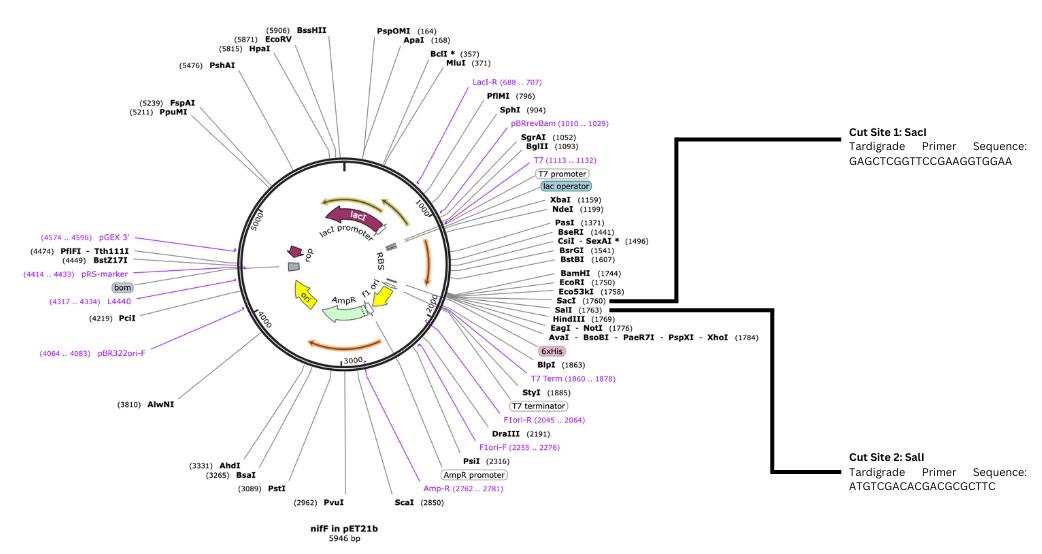
Plasmids (nifF in pET21b), as shown in Figure 1, were purchased from AddGene and were placed in the refrigerator upon arrival. Plasmids in E. coli were then grown in a Luria-Bertani Broth (LB Broth) and 100 micrograms per milliliter mixture overnight in a shaking water bath at 37 °C.
Additionally, plasmids were also grown in a transformation medium (MgSO4 (1.9718 g/L), CaSO4 (0.0136 g/L), CH5COONH4 (1.1 g/L), glucose (10 g), KH2PO4 (0.25 g/L), K2HPO4 (0.55 g/L), 1.8% agar (18 g), autoclaved for 15 minutes) and 100 μg/mL ampicillin mixture overnight in a shaking water bath at 37 °C to test which medium yielded the best results. Previous work suggested the use of transformation media would increase plasmid overnight growth for Azotobacter vinelandii (Natzke et al., 2018). Those in the transformation medium did not grow, but those in LB Broth did.
Overnight cultures were mini-prepped using the NEB #T1010S kit and protocol. A sequential digest using Sac1-HF and Sal-1-HF enzymes from NEB was performed to prepare plasmids for uptake of the CAHS-89226 gene. The sequential digest was composed of 11 μL of nuclease-free water, 2 μL of 1x rCutSmart buffer, 1 μL of enzyme (SacI-HF or Sal-I-HF), and 5 μL of plasmid DNA. The digest
Figure 1. nifF in pET21b plasmid with cut sites, enzyme names, and tardigrade primer sequences. Image of plasmid taken from Addgene and cut sites added by author.
reaction mixture containing Sal-I-HF was incubated at 37 °C for 15 minutes and heat-inactivated at 65 °C before Sac-I-HF was added to the tube. Due to the compatible buffer between both enzymes, a PCR and DNA Cleanup (NEB #T1130) were not used between digestion reactions. Subsequently, a CIP (Calf Intestinal Alkaline Phosphatase) was performed with 6 μL of nuclease-free water, 3 μL of 1x rCutSmart buffer, and 1 μL of CIP enzyme (NEB). This enzyme reaction tube was then incubated at 37 °C for 10 minutes, and 80 °C for 2 minutes to heat-inactivate the enzyme.
Post-CIP, a gel was run to confirm the quality and concentration of the plasmid, and a PCR and DNA Cleanup (NEB #T1030S) was used to isolate the opened plasmid DNA from the reagents and enzymes and then was used to ligate.
2.7 Ligation
Six ligations were done: three different insert ratios of vector:insert (1:1, 1:3, and 1:6), a vector-only, and a plasmid-only. Plasmid-only was used to confirm the success of the electroporation protocol, vector-only was used to confirm the success of the CIP and sequential digest, and insert ratios were used as the desired endproduct of the transformations.
All ligation reaction mixtures included 1 μL vector (opened plasmid DNA), 1 μL T4 DNA Ligase (NEB), 2 μL T4 DNA Ligase Buffer (1x), and varying amounts of nuclease-free water, and insert based on the insert ratio.
Ligation reactions were incubated at room temperature for 10 minutes, inactivated at 65 °C for 10 minutes, and chilled on ice for 5 minutes. Ligations were then cleaned using a PCR and DNA Cleanup Kit from NEB (#T1030S) and stored at -20 °C until use.
2.8 Preparation of Electrocompetent Azotobacter vinelandii
To make Azotobacter vinelandii electrocompetent, cells were cultivated with vigorous shaking in a water bath at 30 °C for two hours. Cells were then harvested by centrifugation at 5000 rpm and 4 °C for 10 minutes. The supernatant was removed and cells were washed and resuspended with an original culture volume of icecold 10% glycerol. Cells were then centrifuged again for 10 minutes at 5000 rpm and 4 °C. This step was repeated three times using half and a quarter of the original volume, and finally 2-4 mL of the glycerol solution.
After harvesting, cells were placed into 0.8 μL microcentrifuge tubes as 40 μL aliquots and stored at -26 °C until electroporation.
2.9 Preparation of Electrocompetent Escherichia coli
To make electrocompetent Escherichia coli, 100 μL of overnight E. coli was inoculated in 10 mL of LB Broth and left to sit for 2-3 hours. Cells were then pelleted by centrifugation for 5 minutes at 6000 RPM and 4 °C. The supernatant was discarded and cells were resuspended in 10 mL of ice-cold 10% glycerol. Cells were centrifuged again for 5 minutes at 6000 rpm and 4 °C. This step was repeated four more times and then resuspended in 100 μL of ice-cold 10% glycerol.
After harvesting, cells were placed into 0.8 μL microcentrifuge tubes as 40 μL aliquots and stored at -26 °C until electroporation.
2.10 Electroporation
For electroporation, electrocompetent cells were thawed on ice. Each sample had a 1.5 mL microcentrifuge tube with SOC Medium (NEB) and an electroporation cuvette placed on ice. In the aliquoted cell tubes, 5 μL of ligated recombinant plasmid was added and incubated on ice for a minute. All the sample was then transferred to a cold electroporation cuvette and inserted into the shock pod of the Gene Pulser XCell. The 1 mm cuvette, E. coli pre-set protocol was used, and cells were pulsed once. Immediately after, 1 mL of cold Extra-Rich Burk’s Medium or SOC Medium (NEB) for A. vinelandii and E. coli, respectively, was added to resuspend cells. Then, the cell suspension was transferred to the 1.5 mL microcentrifuge tube and left to incubate overnight in a shaking water bath of 225 rpm at 37 °C.
The next morning, cells were placed onto Burk’s Medium Agar + 100 μg/mL ampicillin or LB Agar + 100 μg/mL ampicillin plates (for A. vinelandii and E. coli, respectively). Plates were incubated at 37 °C overnight and swabbed the following day to grow selectively in Burk’s Medium with 100 μg/mL ampicillin or LB Broth with 100 μg/mL ampicillin. Cultures were incubated in a shaking water bath at 37 °C overnight.
2.11 Preparation of Chemically Competent Escherichia coli
Lyophilized E. coli K-12 HB101 (Bio-Rad) was rehydrated with LB Broth and incubated overnight as instructed in the Bio-Rad pGLO lab. Cells were then placed in 250 μL of transformation solution (CaCl2), and vortexed. Cells were now ready to use.
2.12 Heat Shock
In the cells and transformation solution mixture, 10 μL of ligated plasmid was added and incubated on ice for 10 minutes, per the pGLO lab Quick Guide. Tubes were then heat-shocked at 42 °C for 50 seconds, followed by an ice bath for 2 minutes. Subsequently, 250 μL of LB Broth was added, and tubes were incubated at room temperature for 10 minutes. Bacteria were resuspended, and 100 μL of cell suspension was plated on selective agar plates.
Plates were incubated at 37 °C overnight and swabbed the following day to grow selectively in Burk’s Medium with 100 μg/mL ampicillin or LB Broth with 100 μg/mL ampicillin. Cultures were incubated in a shaking water bath at 37 °C overnight.
2.13 Miniprep and Gel Electrophoresis Confirmation
For confirmation, 2 mL of each selective liquid culture was miniprepped using the NEB #T1010 kit. Miniprep product was then double digested with Sac-I-HF and SalI-HF (NEB). The double digest reaction mixture contained 5 μL DNA, 2 μL 1X rCutSmart Buffer, 1 μL Sal-I-HF, 1 μL Sac-I-HF, and 11 μL nuclease-free water to make a 20 μL reaction tube. Tubes were placed in VeritiPro 96-Well ThermoCycler and allowed to incubate for 15 minutes at 37 °C. A CIP was performed to ensure no re-ligation between insert and plasmid, and then a 2.5% gel was run to confirm plasmid insertion and insert into A. vinelandii and E. coli.
2.14 Desiccation and Survival Assay for Azotobacter vinelandii
Burk’s Buffer plates (MgSO4 (0.2 g/L), K2HPO4 (0.8 g/L), KH2PO4 (0.2 g/L), CaSO4 (0.13 g/L), FeCl3 (0.00145 g/L), Na2MoO4 (0.000253 g/L), N-Butanol (1-Butanol) (15 μL/L), agar (20 g/L)) were also created for the desiccation protocol. Azotobacter from the new batch was then plated, covered in aluminum foil, and then placed in a dark storage closet for five weeks. When retrieved, Burk’s Buffer plates showed signs of cyst formation. All plated samples were re-suspended in Burk’s Medium and allowed to grow for 2 weeks. An OD-620 was then performed to quantify growth post-desiccation. Post-electroporation and confirmation, new cultures of Azotobacter vinelandii were plated onto Burk’s Buffer plates, covered in aluminum foil, and placed in a dark storage closet for five weeks. When retrieved, Burk’s Buffer plates showed signs of cyst formation, like the control plates. All plated samples were re-suspended in Burk’s Medium and allowed to grow for two weeks. An OD-620 was then performed to quantify growth postdesiccation.
2.15 Desiccation and Survival Assay For Escherichia coli
Overnight cultures of E. coli in LB Broth (control) and LB + Amp Broth (electroporated E. coli) were created and placed in a shaking water bath at 37 °C. All cultures were then diluted to an OD-620 reading of 0.2. Diluted samples were centrifuged at 10,000g for 5 minutes. The supernatant was then discarded and replaced by 100 μL of sterile water. Cells were gently vortexed to resuspend and then placed in a desiccator with silica gel for 1 hour. E. coli was rehydrated using 900 μL LB Broth, and vortexed gently to resuspend the cells. The cell suspension was then incubated at 37 °C for one hour in a shaking water bath to allow for recovery. Finally, OD-620 values were measured to determine cell viability and significance of CAHS-89226.
For controls, diluted samples were centrifuged at 10,000g for 5 minutes, and the supernatant was discarded. Cells were then re-suspended in 900 μL LB Broth and incubated at 37 °C for one hour in a shaking water bath. After, OD-620 values were taken from each sample.
2.16 Data Analysis
Data were analyzed in RStudio using the car, ggplot2, and dplyr packages. For the A. vinelandii desiccation survival assay, a Shapiro-Wilk’s test was used to check for normality for each group, a Levene’s test for equal variances, and a Welch’s Two Sample T-Test to determine the significance between the desiccated, post-electroporation desiccated, and non-desiccated test groups. For the E. coli desiccation survival assay, an ANOVA was used to identify significant differences between the different groups, and then a Tukey’s posthoc was used to analyze statistical differences between individual groups. Following, graphs were created, with standard error bars and significant differences starred.
3. Results
3.1 PCR and Gel Extraction Results For Extraction of CAHS-89226 Gene
As shown in Figure 2, gel electrophoresis was performed on a 1% agarose gel at 100 V for 30 minutes to verify the presence and size of the CAHS-89226 gene. The gel was stained with Gel Loading Dye (NEB #B7025) for visualization, and a DNA ladder (NEB) served as a size reference alongside a negative control that lacked the gene. A distinct band appeared at approximately 250 bp in the CAHS-89226 lane, confirming the successful amplification and extraction of the gene, which was
absent in the control lane.
Figure 2. 1% gel electrophoresis of CAHS-89226 gene with sticky ends and negative control. Image taken by author.
3.2 Plasmid Extraction Gel
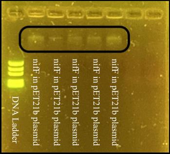
In Figure 3, gel electrophoresis was conducted on a 1% agarose gel at 100 V for 30 minutes to verify the presence of the nifF plasmid obtained from Addgene. The gel was stained with Gel Loading Dye (NEB #B7025) for visualization, with a DNA ladder (NEB) included as a size reference. A distinct band at approximately 6000 bp was observed in nearly all lanes, confirming the expected size of the plasmid. Samples consisted of equal volumes of miniprep and double digest products from overnight cultures of E. coli containing the plasmid in LB broth.
Figure 3. 1% gel electrophoresis of nifF plasmid in pET21b post-miniprep and double digestion. Image taken by author.
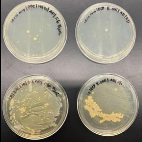
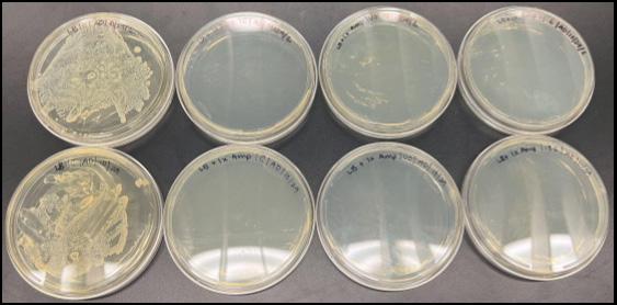
Figure 4 shows LB agar plates (bottom row) are a control to confirm cell viability post-electroporation, showing that cells survived and proliferated. The LB agar + ampicillin plates (top row) test for plasmid transformation; the presence of colonies indicates successful transformation through electroporation. However, as discussed in Section 3.5, the transformed colonies did not incorporate the insert gene.
Figure 4. Electroporated E. coli with a 1:6 plasmid:insert ratio plated on LB agar + 100 μg/mL ampicillin (top row) and LB agar (bottom row). Image taken by author.
3.4 Azotobacter vinelandii Electroporation
Results Post-Plating
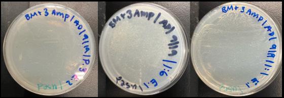
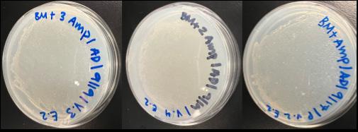
Figure 5 shows the growth of A. vinelandii in every plate as expected in a successful transformation - the presence of the plasmid causes growth in all plates, as the plasmid contains the ampicillin resistance gene.
Figure 5. Electroporated plasmid without insert, 1:6 concentration, and 1:1 concentration in Azotobacter vinelandii plates of Burk’s medium agar and ampicillin stock solution of 300 μg/mL. Images taken by the author.
In Figure 6, the presence of A. vinelandii on all vectoronly plates at varying concentrations of ampicillin suggests the presence of a closed plasmid, suggesting that either the sequential digest or the CIP did not work.
Figure 6. Open vectors in Azotobacter vinelandii on plates of Burk’s medium agar and ampicillin stock solution of 100, 200, and 300 μg/mL. Images taken by author.
3.5
Escherichia
coli
Heat Shock Results Post-Plating
In Figure 7, the LB agar plates suggest cell viability during the heat-shock protocol, as all control groups displayed growth. However, no growth was observed on any LB agar + ampicillin plates, indicating that transformation was unsuccessful. The Control (no plasmid) plate on LB agar + ampicillin showed no growth, confirming ampicillin efficacy. The absence of colonies on the Vector Only and 1:6 plasmid:insert plates suggests two possibilities: either transformation or ligation was unsuccessful.
Figure 7. Heat-shocked E. coli plated on LB agar (column 1) and LB agar + 100 μg/mL ampicillin (columns 2-4). The top row follows an extended heatshock protocol, while the bottom uses the Bio-Rad Quick Guide protocol. All plates contain HB101 E. coli (K-12 strain) from the Bio-Rad pGLO kit. From left to right, the plates include Control (no plasmid) on LB agar, Control (no plasmid) on LB agar + ampicillin, Vector Only (no insert) on LB agar + ampicillin, and 1:6 plasmid:insert on LB agar + ampicillin. Image taken by author.
3.6 Plasmid Extraction Gel Post-Electroporation (For Transformation Confirmation)
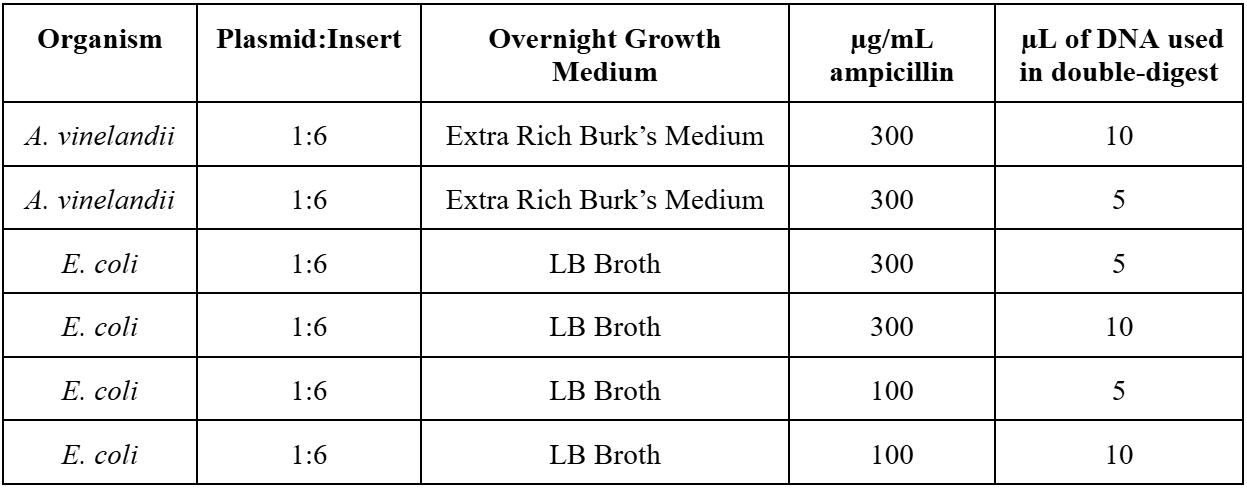
Figure 8 shows a gel electrophoresis performed on a 2.5% agarose gel at 100 V for 30 minutes to confirm the presence of the nifF plasmid in electroporated A. vinelandii and E. coli. The gel was stained with Gel Loading Dye (NEB #B7025) for visualization, and a DNA ladder
(NEB) was included as a size reference. A distinct band appeared at approximately 6000 bp in almost all lanes, confirming the expected size of the plasmid. The samples were loaded as show in Table 1.
Figure 8. 2.5% gel electrophoresis of nifF plasmid grown overnight in varying concentrations of ampicillin and growth medium for Azotobacter vinelandii and Escherichia coli. Image taken by author.
Table 1. Growth conditions for A. vinelandii and E. coli cultures with varying plasmid ratios and DNA concentrations. Table created by the author.
The results confirm the successful transformation of the nifF plasmid into A. vinelandii and E. coli; however, they also indicate that the insert is not present in the plasmid.
3.7 Azotobacter vinelandii Desiccation And Survival Assay
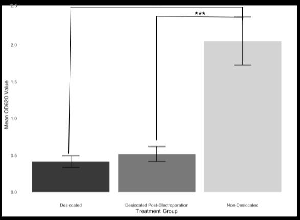
Statistical analysis revealed significant differences in OD-620 values between the desiccated and nondesiccated groups (p = 3.7e-16) and between the desiccated post-electroporation and non-desiccated groups (p = 3.0e-14) in Figure 9. However, no significant difference was found between the desiccated and desiccated post-electroporation groups (p = 0.41), likely due to an incomplete double digest that prevented the plasmid from accepting the insert gene. Despite this, the data suggest that the desiccated post-electroporation groups exhibited slightly higher tolerance, indicating that A. vinelandii cell viability and cyst formation ability are not adversely affected by the electroporation process or the introduction of the nifF gene.
9. Graph of mean OD-620 values for desiccated (n=10), desiccated post-electroporation (n=5), and non-desiccated treatment groups (n=7). Graph created in RStudio by author.
3.8 Escherichia coli desiccation and survival assay
In Figure 10, the lack of significant differences between the desiccated electroporated cells and desiccated control groups can be attributed to an incomplete double digest, preventing the plasmid from accepting the insert gene. Gel electrophoresis results confirmed these findings, with a band at approximately 6000 bp for the plasmid, but none around 250 bp for the cut insert gene. Interestingly, unlike in A. vinelandii, desiccated electroporated cells had lower cell viability than the desiccated controls significantly. This suggests that E. coli cell viability and cyst formation ability remain unaffected by electroporation or the introduction of the nifF gene in the pET21b plasmid.
Figure
Figure 10. Graph of mean OD-620 values for desiccated (n=6), desiccated post-electroporation (n=6), non-desiccated (n=8) and non-desiccated post-electroporation (n=8) treatment groups.
4. Discussion
This study investigated the use of the CAHS-89226 gene in the desiccation tolerance of tardigrades. The protocol followed consisted of three main parts: gene extraction, recombinant plasmid creation with insert, and subsequent survival assays to test desiccation tolerance.
4.1 Successful Extraction of CAHS-89226 from Hypsibius exemplaris
Though H. exemplaris is widely used in laboratories, its entire genome has neither been sequenced nor annotated, leading to only a 93% confidence in the existence of CAHS-89226 within the genome (Hypsibius Exemplaris Genome Assembly nHd_3.1, n.d.). For this reason, extracting the gene proved difficult, as not all primers were consistently and accurately able to extract the gene. Thus, the successful extraction of CAHS-89226 opens the door to future uses of the gene in other projects.
4.2 Implications of the Survival Assays
In Azotobacter vinelandii, the significant differences between the desiccated and non-desiccated groups suggest that desiccation, while possible, greatly harms the A. vinelandii population, and not all survive. Additionally, the insignificant differences between the dessicated post-electroporation and desiccated groups suggest that the plasmid had no effect on desiccation tolerance on its own. Moreover, the insignificant difference between the desiccated post-electroporation and desiccated groups suggests the viability and non-impaired desiccation tolerance of A. vinelandii cells post-electroporation.
In Escherichia coli, the significant differences between the desiccated and non-desiccated groups suggest that desiccation, while possible, significantly harms
E. coli populations, with very select few surviving. The insignificant difference between the desiccated postelectroporation and desiccated groups suggests nonimpaired cell viability post-electroporation and also suggests that the plasmid did not accept the insert.
4.3
Limitations
4.3.1
Gene Interactions
Due to time constraints, this study examined CAHS89226 in isolation, though it’s known that tardigrade desiccation tolerance often relies on the collaborative effects of multiple genes, such as LEA-1 and SAHS. Future studies should investigate CAHS-89226 alongside other desiccation tolerance genes to understand their combined role in stress response and survival mechanisms.
4.3.2
Absence of Trehalose
Although trehalose is often co-expressed with CAHS proteins to enhance desiccation tolerance, it was not used in this protocol. Since trehalose may work synergistically with CAHS genes, its absence could have limited the observable effects of CAHS-89226 in this study. Due to the previously studied positive relationship between trehalose and CAHS, it can be assumed that desiccation tolerance would improve.
4.3.3 Host Limitations
E. coli and A. vinelandii may not be optimal models for studying tardigrade genes, as they lack cellular pathways and molecular structures native to eukaryotes like tardigrades. Future research could consider alternative hosts or in vitro systems better suited for examining the desiccation resilience expressed by tardigrade genes. Despite these limitations, the study provides a foundational understanding of CAHS-89226’s potential role in desiccation tolerance and highlights several pathways for further investigation.
5. Conclusion, Implications, and Future Work
5.1 Conclusion
This study aimed to advance the understanding of the role of CAHS-89226 in desiccation tolerance by isolating the gene from Hypsibius exemplaris and inserting it into Escherichia coli and Azotobacter vinelandii for desiccation survival assays. The successful extraction of the CAHS89226 gene brings the scientific community a step closer to understanding the use of the TDPs in cryptobiosis of tardigrades. Additionally, the extraction also confirms
the existence of the CAHS-89226 gene in H. exemplaris, as the organism has not been sequenced, leading to doubt in the existence of certain genes.
5.2
Implications and Future Work
This research lays essential groundwork for future studies on desiccation tolerance in H. exemplaris and uncovers broader potentials for cross-species application of stress tolerance genes. Additionally, it allows for future cloning studies of the CAHS-89226 gene, improving understanding of TDPs, as well as possibly improving the anhydrobiotic capabilities of other organisms.
Engineering desiccation-tolerant organisms could have far-reaching applications in the future. Since tardigrades, from which CAHS-89226 was derived, can pause aging in extreme conditions, this gene may similarly affect cellular aging in other species. Further studies should examine whether CAHS-89226 can modulate aging processes, potentially paving the way for its use in space travel, where paused aging could make long-term missions more feasible through the reduction of the need for resources and detrimental health effects from being active in space.
6. Acknowledgements
I would like to express my heartfelt gratitude to Dr. Heather Mallory for all her support. It has meant more to me than I can express. I am also deeply thankful to Dr. Kimberly Monahan for sharing her expertise in molecular genetics.
To the NCSSM RBio Class of ‘25, thank you for your encouragement, humor, and hope—you have all inspired me to push my limits and pursue a research career.
Finally, I would like to acknowledge the NCSSM Foundation, the Burroughs Wellcome Fund, and GlaxoSmithKline for their generous funding. This project would not have been possible without your support.
7. Works Cited
Barilla, M. A., Shuster, S. O., & Davis, C. (2024). Tardigrade CAHS hydrogels protect proteins through concentrationdependent mechanism. Biophysical Journal, 123(3), 75a–76a.
Boothby, T. C., Tapia, H., Brozena, A. H., Piszkiewicz, S., Smith, A. E., Giovannini, I., Rebecchi, L., Pielak, G. J., Koshland, D., & Goldstein, B. (2017). Tardigrades use intrinsically disordered proteins to survive desiccation. Molecular Cell, 65(6), 975-984.e5.
Buckey, J. C., Phillips, S. D., Anderson, A. P., Chepko, A. B., Archambault-Leger, V., Gui, J., & Fellows, A. M. (2018). Microgravity-induced ocular changes are related to body weight. American Journal of Physiology-Regulatory, Integrative and Comparative Physiology, 315(3), R496.
Castillo, T., García, A., Padilla-Córdova, C., Díaz-Barrera, A., & Peña, C. (2020). Respiration in Azotobacter vinelandii and its relationship with the synthesis of biopolymers. Electronic Journal of Biotechnology, 48, 36–45.
Cryonics | Description, Process, Popularization, & Facts | Britannica
Ekpo, M. D., Boafo, G. F., Gambo, S. S., Hu, Y., Liu, X., Xie, J., & Tan, S. (2022). Cryopreservation of Animals and Cryonics: Current Technical Progress, Difficulties and Possible Research Directions. Frontiers in Veterinary Science, 9.
Escherichia Coli K 12—An overview | ScienceDirect Topics. (n.d.-a).
Garbacki, N., Willems, J., Neutelings, T., Lambert, C., Deroanne, C., Adrian, A., Franz, M., Maurer, M., De Gieter, P., Nusgens, B., & Colige, A. (2023). Microgravity triggers ferroptosis and accelerates senescence in the MG-63 cell model of osteoblastic cells. Npj Microgravity, 9(1), 1–16.
Gąsiorek, P., Stec, D., Morek, W., & Michalczyk, Ł. (2018). An integrative redescription of Hypsibius dujardini (Doyère, 1840), the nominal taxon for Hypsibioidea (Tardigrada: Eutardigrada). Zootaxa, 4415(1), 45–75.
Hashimoto, T., Horikawa, D. D., Saito, Y., Kuwahara, H., Kozuka-Hata, H., Shin-I, T., Minakuchi, Y., Ohishi, K., Motoyama, A., Aizu, T., Enomoto, A., Kondo, K., Tanaka, S., Hara, Y., Koshikawa, S., Sagara, H., Miura, T., Yokobori, S., Miyagawa, K., Kunieda, T. (2016). Extremotolerant tardigrade genome and improved radiotolerance of human cultured cells by tardigrade-unique protein. Nature Communications, 7(1), 12808.
Hibshman, J. D., Clegg, J. S., & Goldstein, B. (2020). Mechanisms of Desiccation Tolerance: Themes and Variations in Brine Shrimp, Roundworms, and Tardigrades. Frontiers in Physiology, 11.
Jenkins, J. M., Twicken, J. D., Batalha, N. M., Caldwell, D. A., Cochran, W. D., Endl, M., Latham, D. W., Esquerdo, G. A., Seader, S., Bieryla, A., Petigura, E., Ciardi, D. R., Marcy, G. W., Isaacson, H., Huber, D., Rowe, J. F., Torres, G., Bryson, S. T., Buchhave, L., Borucki, W. J. (2015). Discovery and validation of Kepler-452b: a 1.6 R super earth exoplanet in the habitable zone of a G2 star. The Astronomical Journal, 150(2), 56.
Joseph, A. (2023). Chapter 5—Extremophiles— Organisms that survive and thrive in extreme environmental conditions. In A. Joseph (Ed.), Water Worlds in the Solar System (pp. 201–254). Elsevier.
Kasianchuk, N., Rzymski, P., & Kaczmarek, Ł. (2023). The biomedical potential of tardigrade proteins: A review. Biomedicine & Pharmacotherapy, 158, 114063.
Katsuyama, Y. (2019). Microbial Type III Polyketide Synthases. In Reference Module in Chemistry, Molecular Sciences and Chemical Engineering. Elsevier.
Lim, S., Reilly, C. B., Barghouti, Z., Marelli, B., Way, J. C., & Silver, P. A. (2024). Tardigrade secretory proteins protect biological structures from desiccation. Communications Biology, 7(1), 1–10.
Lv, H., Yang, H., Jiang, C., Shi, J., Chen, R., Huang, Q., & Shao, D. (2023). Microgravity and immune cells. Journal of the Royal Society Interface, 20(199).
Man, J., Graham, T., Squires-Donelly, G., & Laslett, A. L. (2022). The effects of microgravity on bone structure and function. Npj Microgravity, 8(1), 1–15.
Møbjerg, N., & Neves, R. C. (2021). New insights into survival strategies of tardigrades. Comparative Biochemistry and Physiology Part A: Molecular & Integrative Physiology, 254.
Moon to Mars Architecture—NASA (2024).
Natzke, J., Noar, J., & Bruno-Bárcena, J. M. (2018). Azotobacter vinelandii nitrogenase activity, hydrogen production, and response to oxygen exposure Applied and Environmental Microbiology, 84(16), e01208-18.
Nguyen, K., Kc, S., Gonzalez, T., Tapia, H., & Boothby, T. C. (2022a). Trehalose and tardigrade CAHS proteins work synergistically to promote desiccation tolerance. Communications Biology, 5(1), Article 1.
Noar, J. D., & Bruno-Bárcena, J. M. (2018a). Azotobacter vinelandii: The source of 100 years of discoveries and many more to come. Microbiology (Reading, England), 164(4), 421–436.
Poprawa, I., Bartylak, T., Kulpla, A., Erdmann, W., Roszkowska, M., Chajec, Ł., Kaczmarek, Ł., Karachitos, A., & Kmita, H. (2022). Verification of Hypsibius exemplaris (Eutardigrada; Hypsibiidae) application in anhydrobiosis research. PLoS ONE, 17(3), e0261485.
Rare Diseases. (2020, February 7). National Institutes of Health (NIH).
Rodriguez-Salazar, J., Moreno, S., & Espín, G. (2017a). LEA proteins are involved in cyst desiccation resistance and other abiotic stresses in Azotobacter vinelandii Cell Stress and Chaperones, 22(3), 397–408.
Roszkowska, M., Gołdyn, B., Wojciechowska, D., Kosicki, J. Z., Fiałkowska, E., Kmita, H., & Kaczmarek, Ł. (2021). Tolerance to anhydrobiotic conditions among two coexisting tardigrade species differing in life strategies. Zoological Studies, 60, e74.
Sieger, J., Brümmer, F., Ahn, H., Lee, G., Kim, S., & Schill, R. O. (2022). Reduced ageing in the frozen state in the tardigrade Milnesium inceptum (Eutardigrada: Apochela). Journal of Zoology, 318(4), 253–259.
Tapia, H., Young, L., Fox, D., Bertozzi, C. R., & Koshland, D. (2015). Increasing intracellular trehalose is sufficient to confer desiccation tolerance to Saccharomyces cerevisiae Proceedings of the National Academy of Sciences, 112(19), 6122–6127.
Tardigrade. (2020, March 13). National Geographic.
Vela, G. R. (1974). Survival of Azotobacter in Dry Soil. Applied Microbiology, 28(1), 77–79.
Waisberg, E., Ong, J., Masalkhi, M., Mao, X. W., Beheshti, A., & Lee, A. G. (2024). Mitochondrial dysfunction in Spaceflight Associated Neuro-Ocular Syndrome (SANS): A molecular hypothesis in pathogenesis. Eye, 38(8), 1409–1411.
Wełnicz, W., Grohme, M. A., Kaczmarek, Ł., Schill, R. O., & Frohme, M. (2011). Anhydrobiosis in tardigrades—The last decade. Journal of Insect Physiology, 57(5), 577–583.
Yin, Y., Liu, J., Fan, Q., Zhao, S., Wu, X., Wang, J., Liu, Y., Li, Y., & Lu, W. (2023). Long-term spaceflight composite stress induces depression and cognitive impairment in astronauts—Insights from neuroplasticity. Translational Psychiatry, 13(1), 1–7.
Yoshida, Y., Horikawa, D. D., Sakashita, T., Yokota, Y., Kobayashi, Y., Tomita, M., & Arakawa, K. (2021). RNA sequencing data for gamma radiation response in the extremotolerant tardigrade Ramazzottius varieornatus. Data in Brief, 36.
EFFECTS OF HYPERCHOLESTEROLEMIA AND THE INHIBITION OF THE AGE-RAGE PATHWAY ON EXOPHER FORMATION IN C. ELEGANS
Anneliese Heyder
Abstract
Aggregation of proteins and mitochondrial dysfunction have been linked to neurodegenerative diseases such as Alzheimer’s, Huntington’s, and Parkinson’s across species (Arnold et al., 2020). Exophers are large, membrane-bound vesicles that can sort out neurotoxins or protein aggregates and carry them out of the cell for degradation (Wang et al., 2023). Loss of proteostasis can be the effect of many different stressors; one link researchers have found is elevated cholesterol levels. Abnormally high cholesterol levels in the brain have been linked to multiple neurological disorders such as Parkinson’s, Huntington’s, amyotrophic lateral sclerosis (ALS), and atherosclerosis (Jin et al., 2019). The AGERAGE (Advanced Glycation End Products - Advanced Glycation End Products) signaling pathway leads to the expression of inflammatory cytokines and ROS (reactive oxidation species), which are associated with many neurological disorders (Reddy et al., 2023). In this experiment, the effect of different cholesterol levels on protein aggregation and exopher formation through the AGE-RAGE pathway in C. elegans was investigated. Worms were exposed to cholesterol for 48 hours, and a thrashing and exopher assay was performed. Worms were then exposed to Azeliragon, a RAGE inhibitor, for 24 hours and another thrashing and exopher assay was performed. The results support that cholesterol can induce neurodegeneration by decreasing dopamine levels and that neurotoxins produced by cholesterol cause exophergenesis to become activated and increase production, which is dependent on the AGE-RAGE pathway.
1. Introduction
1.1
Proteostasis in Neuronal Cells
Protein aggregation/accumulation has been shown to promote and spread neurodegenerative toxins among neuronal cells (Arnold et al., 2023). This disrupts proteostasis, the network of biological pathways that regulates protein synthesis and degradation so that cells can reach the required level of protein content for cellular function. Proteostasis is essential for the survival of cells and the degradation of toxic materials, and disruption of this process can lead to the activation of neuroprotective mechanisms like autophagy (degradation and recycling of cellular components) and other genesis. Exophergenesis, a conserved mechanism in C. elegans, involves large vesicles that remove neurotoxins from the brain and deliver them to the hypodermis, where the contents will be degraded. While still largely unknown, this mechanism could be a target for therapeutic manipulation involving neurodegenerative disorders and provide insight into how neurodegeneration spreads in humans (Arnold et al., 2023).
1.2 Stressors and Cholesterol in Neurodegeneration
For exopher production to be increased, proteostasis needs to be challenged. Stressors include oxidative stress,
aging, fasting, or elevated cholesterol levels (Cooper et al., 2021). High cholesterol levels are an effect of highfat diets and obesity, which affect around 1/3 of the US adult population (Freeman et al., 2014). The brain contains about 20% of all the cholesterol in the body, the highest amount for an individual organ (Jin et al., 2019). Abnormal cholesterol levels in the brain have been linked to multiple neurological disorders such as Parkinson’s, Huntington’s, amyloid lateral sclerosis (ALS), and atherosclerosis (Jin et al., 2019). While controversial, many studies have found that changes in normal cholesterol levels can affect neuronal health. For instance, cholesterol loss may help combat neurons’ stress (Rudajev, 2022). High cholesterol levels have also been associated with other neurodegenerative stressors such as autophagy disruption, lysosomal inhibition, oxidative stress, and reduction of mitophagy (Rudajev, 2022)
1.3 Hypercholesterolemia and the AGE-RAGE Pathway
Hypercholesterolemia causes increases in ROS through different mechanisms (increases in oxidative stress and misfolded proteins) and has been linked to increased activation in the AGE-RAGE pathway (McNair et al., 2016). The AGE-RAGE pathway plays an important role in diabetic neuropathy and has been linked to involvement in the pathology of neurodegenerative disorders (Wang
et al., 2023). AGEs (advanced glycation products) have played an important role in many inflammatory health issues, including neurodegenerative disorders like Parkinson’s, Alzheimer’s, and atherosclerosis (Wang et al., 2023). Specifically, ligands that bind to RAGE receptors are the most involved in the pathology of neurodegenerative diseases. The inhibition of these binding ligands is suggested to be the most effective way of reducing the pathology caused by this pathway (Wang et al., 2023). Several studies have shown that AGE-RAGE interactions increase ROS levels by the production of NADPH oxidase. ROS, or reactive oxygen species, are important in the progression and pathology of neurodegenerative diseases (Reddy et al., 2023). This pathway is still poorly understood but may provide a potential therapeutic model for neurological diseases and could be the link in exopher formation.
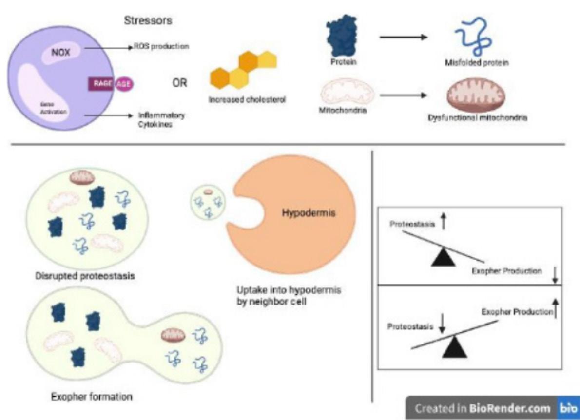
One proposal, as seen in Figure 1, illustrates how stressors such as ROS production, inflammatory cytokines, or elevated cholesterol can lead to misfolded proteins and dysfunctional mitochondria, resulting in the disruption of proteostasis. When proteostasis remains normal, exopher production decreases; when proteostasis is disrupted, exopher production is increased. Once exopher-genesis has been activated through disrupted proteostasis, it can then transport the toxic material to the hypodermis to be degraded. By exposing C. elegans to cholesterol, and inducing neurodegeneration through disruption of proteostasis, exopher production is increased. To understand if AGE-RAGE plays a role in the pathogenesis of exopher formation, a RAGE inhibitor is given to worms with cholesterol-induced neurodegeneration to determine whether exopher production is increased or decreased.
1.4 C. elegans Model
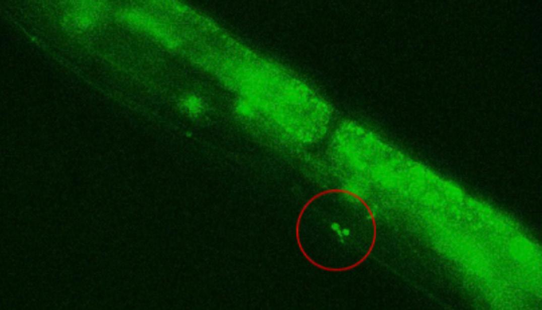
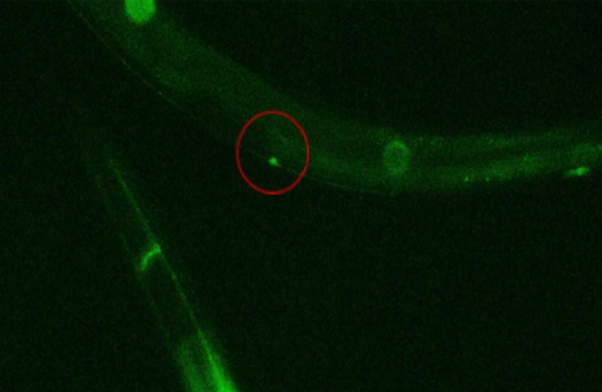
C. elegans is a suitable model for this research due to its simplicity, transparency, and similarities in its neurotransmitters and mechanisms to mammalian models (Sammi et al., 2022). C. elegans has also highlighted several pathway mechanisms involving aging and proteostasis (Arnold et al., 2023). Exophers in C. elegans are produced with most of the material already in the vesicle. A filament can provide even more defective material to the vesicle if needed. Once the exopher is ready for degradation, it detaches from the filament and encounters the hypodermis. A process nicknamed “starry night” then occurs, allowing defective cellular material to be broken down. If the material is still not deteriorated by the hypodermis, coelomocytes can be used to further degrade the components, as shown in Figures 2 and 3 (Arnold et al., 2020). Strain CZ10175 contains GFP (green fluorescent protein) expressed in the 6 neurons
Exophers, which are formed from the soma, also express GFP which allows for them to be easily identified once the 6 main neurons have been located. Through this model organism, this experiment will investigate how cholesterol influences exopher-genesis and the role of the AGE-RAGE pathway in this process.
The ALMR neuron has been shown to produce the most exophers (Arnold et al., 2020), and exophers can normally be found near the soma.
Figure 1. Proposed model of exopher-genesis role in proteostasis and AGE-RAGE pathway. The activation of AGE-RAGE leads to the production of ROS and inflammatory cytokines (both associated with neurodegenerative disorders), and its proposed role in the exopher-genesis process. Produced by the author in Biorender.
Figure 2. Image of C. elegans with exopher taken with fluorescent microscope. The strain CZ10175 allows exophers to glow just as brightly as the six neurons in the nematode. Exophers can range in size from 1/5 the size of a soma (averaging around 3.83 μm) to the size of a neuron (around 6.53 μm) (Arnold et al., 2020). Image taken and produced by author.
Figure 3. Image of ALML neuron in C. elegans taken with fluorescent microscope. There are 6 main neurons in C. elegans, and before scoring for exophers they must be accounted for. Exophers are slightly smaller than somas and are usually attached to the soma with a thin filament.
2. Methods
2.1 C. elegans Maintenance
Standard protocols maintained C. elegans strain N2 and CZ10175 on NGM growth media. CZ10175 C. elegans were maintained at 20°C on consistent media and with consistent bacterial food sources (OP50 E. coli). Strain N2 and CZ10175 were purchased at the University of Minnesota.
2.2 Cholesterol Treatments
Cholesterol treatments included the following concentrations: 0.0 mg/ml, 7.5 mg/mL, 10 mg/mL, and 25 mg/mL. Cholesterol was diluted in ethanol. Prepared cholesterol treatments were mixed in the OP50 and seeded onto NGM plates.
2.3
RAGE Inhibitor Azeliragon Treatment
Azeliragon was dissolved in 1 mL of dimethyl sulfoxide (DMSO) and then dissolved in 4 mL of lysogeny broth (LB) for a final concentration of 20% Azeliragon. 50 µL were pipetted onto plates and were allowed to dry before transferring worms. C. elegans were exposed to Azeliragon for 24 hours before being assayed.
2.4
Thrashing Assay
Thrashing assays were performed using 2% agar solution, microscope slide, and M9 buffer. The 2% agar solution was heated until melted, and a drop was placed onto a clean microscope slide and compressed with
an additional slide. Once dry, 10 μL of M9 buffer were pipetted onto the slide. C. elegans were picked onto the slide and then videoed with a Lumenara Microscope Camera. Thrashes were recorded for 15 seconds. Assays were blinded.
2.5 Exopher Imaging
C. elegans were immobilized with a sodium azide solution to count exophers effectively. Exophers were scored with a ‘yes’ or ‘no’. Exopher production was highest on larva adult days 2-3 but could appear at any time in the life cycle. Orientation of worms was determined and fluorescent neurons were observed using 100x magnification with a fluorescent dissecting microscope. Paralyzed animals were mounted to identify neurons and specific exophers, and the 6 neurons were identified to find localized exophers.
2.6 Statistics
A Shapiro-Wilk test was used to determine normality for thrashing assays. If the test was normally distributed, an ANOVA was performed to determine if groups were statistically significant from each other. If data were abnormally distributed, a Kruskal-Wallis test was used to determine if there were significant differences between two or more groups. A Tukey’s Honestly Significant Difference (HSD) test was performed to understand what groups were significantly different from each other. Exopher imaging was analyzed using a binomial test. Data analysis was done using RStudio, and AI was utilized in coding for data analysis. Blinding was done by labeling thrashing assay videos and having a peer rearrange them so groups with cholesterol and no cholesterol treatments were not in a known order.
3. Results
3.1 Cholesterol Thrashing Assays
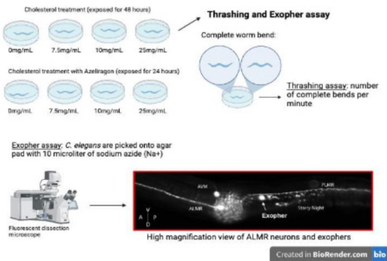
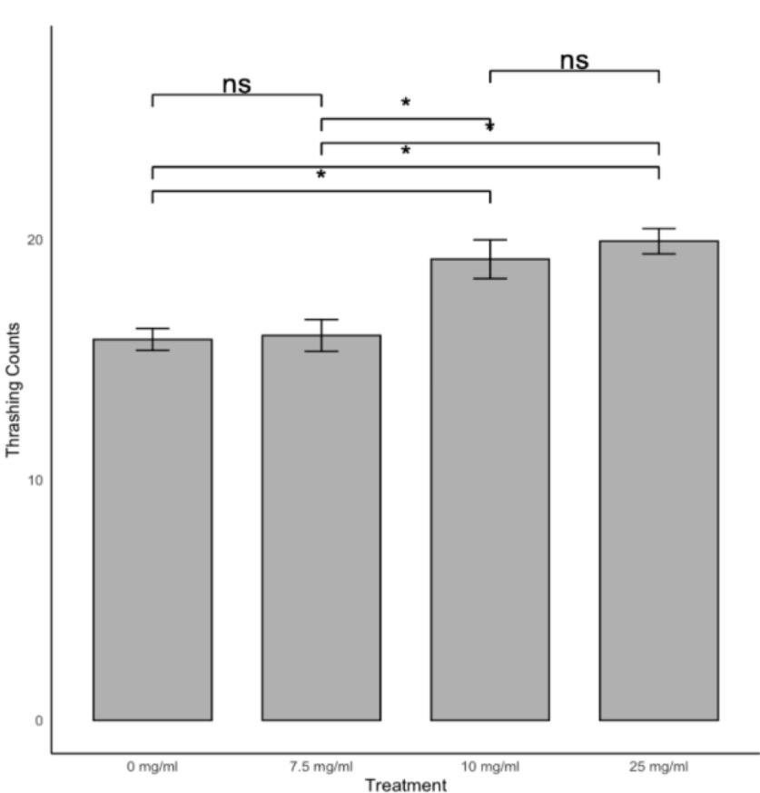
To determine if cholesterol caused neurodegeneration, C. elegans were exposed to different levels of cholesterol for 48 hours and underwent a thrashing assay to determine if dopamine-induced neurodegeneration had occurred as shown in Figure 4. Figure 5 shows the average thrashing counts of worms exposed to different levels of cholesterol. There were no significant differences between treatment groups 0 mg/mL and 7.5 mg/mL of cholesterol; however, there was a significant increase in the thrashing rate of 10 mg/mL and 25 mg/mL when compared to both 0 mg/mL and 7.5 mg/mL. Cholesterol treatment of 10 mg/mL and 25 mg/mL had an average thrashing rate of 19.2 and 19.9 thrashes/15 seconds respectively as compared to 0mg/
mL and 7.5 mg/mL with an average thrashing rate of 15.8 and 16.0 thrashes/15 seconds, as shown in Figure 5.
Figure 4. Methods and protocol for treatment and assays. Procedure shows the different cholesterol treatments, exposure time, and a brief description of each assay performed. Made by the author using Biorender.
Figure 5. Hypercholesterolemia thrashing assay. Mean ± SE thrashes per 15 seconds for worms exposed to different concentrations of cholesterol for 48 hours (n=12 for all groups). One-way ANOVA was performed as well as Tukey’s test to understand the significance between groups. F = 6.3, which indicates a higher variability and more evidence to reject the null hypothesis. Produced by author in RStudio. (* : p < 0.05, ** : p < 0.01, *** : p < 0.001, ns : p> 0.05)
3.2 Azeliragon Thrashing Assays
To determine if cholesterol-induced neurodegeneration was dependent on the AGE-RAGE pathway, C. elegans were exposed to RAGE inhibitor Azeliragon for 24 hours after exposure to elevated cholesterol levels for 48 hours. Thrashing was then blinded, recorded, and compared to the thrashing of just cholesterol. Exposure to Azeliragon caused thrashing to decrease for all groups except the one exposed to no cholesterol (0 mg/ml) (Fig. 6). The control group (0 mg/ml) and the 10 mg/ml group were not significant, but both the 7.5 mg/ml and 25 mg/ml were significant when compared to their paired groups with exposure to Azeliragon. Worms exposed to no cholesterol and no cholesterol + Azeliragon had the lowest average thrashing of 16.9 thrashes per 15.0 seconds and 18.9 thrashes per 15.0 seconds.
Figure 6. Thrashing assays of groups exposed to cholesterol and cholesterol and Azeliragon. Mean ± SE thrashes per 15 seconds when exposed to different cholesterol levels for 48 hours and when exposed to Azeliragon for 24 hours (n=12 for all treatment groups). A Shapiro-Wilks test was performed to understand normality, and a t-test was done to show significance between treatment groups. Produced by the author in RStudio. F =3.2 (0 mg/ml and 0 mg/ml + AZE), F = 18.9 (7.5 mg/ml and 7.5 mg/ml + AZE), F = 1.2 (10 mg/ml and 10 mg/ml + AZE), F = 5.1 (25 mg/ml and 25 mg/ml + AZE). (* : p < 0.05, ** : p < 0.01, *** : p < 0.001, ns : p> 0.05)
3.3 Cholesterol-Induced Exopher-Genesis
Exopher-genesis was imaged and analyzed to determine if exophers formed from cholesterol stress were dependent on the AGE-RAGE pathway. C. elegans
were exposed to no cholesterol, 10 mg/mL cholesterol, or 10 mg/ml + Azeliragon. Exophers were scored binomially, with a ‘yes’ or a ‘no’. Figure 7 represents the percentage of C. elegans that had an exopher. The control group (0 mg/ml) had 8% of worms with exophers, the cholesterol treatment group had 26% of worms with exophers and when exposed to Azeliragon that number decreased to 6%. Both the control group and the Azeliragon group had significant differences compared to the group exposed to just cholesterol (10 mg/mL). The control group and the Azeliragon group were not significantly different.
Figure 7. Exopher assay counts of groups exposed to cholesterol and cholesterol Azeliragon. Percentage ± SE of worms with exophers when exposed to different cholesterol levels and RAGE inhibitor Azeliragon (n=50 for all treatment groups). A binomial test was performed for analysis. Produced by the author in RStudio. (* : p < 0.05, ** : p < 0.01, *** : p < 0.001, ns : p> 0.05)
4. Discussion
4.1 Effects of Cholesterol on Dopamine Neuron Function and Exopher-Genesis
C. elegans were exposed to different cholesterol concentrations, and thrashing for each worm (n=15) was counted for 15 seconds. Results show that thrashing increased when exposed to increased cholesterol levels (see Figure 5). Thrashes are regulated by a dopaminesignaling pathway (Sanyal et al., 2004), and are indirectly related to the concentration of dopamine in C.
elegans; as dopamine levels decrease, thrashing increases. Cholesterol-induced stress can cause dopamine production to decrease, therefore resulting in increased thrashing. Higher cholesterol levels increase oxidative stress, producing dysfunctional mitochondria and misfolded proteins (Rudajev, 2022); once the neurons in C. elegans begin experiencing this disruption of proteostasis, exopher production is increased. Instead of testing different cholesterol levels on exopher production, treatments were narrowed down to 10 mg/mL of cholesterol to imitate a more realistic level of cholesterol. 10 mg/mL of cholesterol had very similar thrashing results to the group exposed to 25 mg/mL, as shown in Figure 5. Results indicate that increased cholesterol does result in higher exopher production compared to no added cholesterol (0 mg/mL), supporting that exopher production is activated when stress is increased. This indicates a relationship to neurons experiencing proteostress.
4.2 Role of AGE-RAGE Pathway in Exopher-Genesis
RAGE can be found in many cells, including neurons. It can bind to different ligands, one being AGE, which can lead to the generation of ROS (Pinkas et al., 2018). This binding pathway may be a potential pathway to investigate exopher production and regulation. Activation of this pathway results in neurotoxins such as ROS and cytokines, both of which could activate exopher production. To determine if exopher production is involved or can be regulated with this pathway, C. elegans were exposed to cholesterol for 48 hours and then exposed to an AGE-RAGE inhibitor (Azeliragon) for 24 hours.
Thrashing and exopher assays were both performed. Thrashing was done to show that the AGE-RAGE pathway can decrease motility, resulting in increased dopamine production (see Figure 6). The percentage of C. elegans with exophers decreased when exposed to Azeliragon, indicating lower exopher production (see Figure 7). This indicates a relationship between the AGE-RAGE pathway and exopher production, which may be a potential answer when investigating what other biological systems play a role in exopher production.
4.3 Exopher Role in Neurodegeneration
Exophers are considered to be neuroprotective, helping to discard neurotoxins and other harmful products that may disrupt proteostasis. However, scientists have posed the idea that exophers could be contributing to the leakage of these neurotoxins, essentially leading to the spread of neurodegeneration (Arnold et al., 2023). While further research is needed for this question, the data in this paper support the idea that exophers are involved in
neurodegeneration. Exopher production was increased when cholesterol levels were elevated, indicating that exopher production was increased when neurons underwent stress and contributed to the pathogenesis of dopamine-dependent neurons (see Figure 7).
Exopher-genesis is activated when neurons undergo a disruption of proteostasis. The question is whether the production of exophers is neuroprotective or leads to the spreading of neurotoxins between neuronal cells, ultimately contributing to neurodegenerative disorders.
AGE-RAGE inhibition causes thrashing to decrease (Figure 6), effectively preventing dopamine-induced neurodegeneration. It also causes a decrease in exopher production (Figure 7), which supports its role in exopher production and indicates that exophers contribute to the pathogenesis of neurons. This is one of the first studies that support the role of exopher formation and its role in the degeneration of neurons in a cholesterol-induced model.
5. Limitations, Conclusion, and Future Work
Thrashing and exopher assays were performed using a Lumenara Miscrope Camera, which lacks the latest technology and has rather low-quality images. This made getting clear images of exophers difficult and more time was spent than needed on identifying exophers. Strain CZ10175 did show exopher formation, but not the spread of contents which could have provided more insight into how exophers are spreading neurotoxins or degrading them. For this, a strain highlighting “starry night”, the degrading of exophers by the hypodermis, was needed. Finally, strain CZ10175 was identified in previous papers as a strain with low amounts of exophers. Due to this low percentage, a high number of trials (n=50) was done for exopher imaging, which took up a large chunk of time. Unfortunately, a strain with high percentages of exophers could not be found.
Exopher-genesis can provide insight into how neurotoxins are discarded throughout the cell and the importance of proteostasis within neurons. Disruption of this, due to stress, is how neurotoxins are produced and distributed, ultimately leading to the spread of neurodegeneration. By understanding the impacts of exophers, scientists can further investigate how exopher-genesis is activated and whether other stresses are significant in exopher production. Research from this project indicates that cholesterol does cause neurodegeneration through decreased dopamine and that exopher production was increased when C. elegans were put through this stressor. Elevated cholesterol can be associated with disruption of proteostasis and activation of exopher-genesis. Data also indicate that exophers are involved in further neurodegeneration,
and could be a potential model when investigating how neurodegeneration is spread and what signaling pathways are involved.
Future research includes determining what other stressors impact exopher-genesis and the other pathways involved in exopher production. While cholesterol and the AGE-RAGE pathway are shown to affect exopher production, it’s important to understand exactly how exopher-genesis is regulated. Understanding the regulations behind this mechanism can provide more insight into how neurotoxins such as dysfunctional mitochondria and misfolded proteins can be spread and stopped, preventing further disruption of proteostasis and retaining neuronal health.
6. Acknowledgements
I would like to thank my mentors Dr. Kimberly Monahan and Dr. Heather Mallory for their support, guidance, and patience throughout my research. I would also like to acknowledge my Research in Biology peers for their enthusiasm and encouragement. Finally, I would like to give thanks to the Glaxo Endowment and the Burroughs Wellcome Fund for funding my research.
7. Bibliography
Arnold, Meghan Lee, Jason Cooper, Rebecca Androwski, et al. “Intermediate Filaments Associate with Aggresome-like Structures in Proteostressed C. elegans Neurons and Influence Large Vesicle Extrusions as Exophers.” Nature Communications, vol. 14, no. 1, 1, July 2023, p. 4450.
Arnold, Meghan Lee, Jason Cooper, Barth D. Grant, et al. “Quantitative Approaches for Scoring in vivo Neuronal Aggregate and Organelle Extrusion in Large Exopher Vesicles in C. elegans.” JoVE (Journal of Visualized Experiments), no. 163, Sept. 2020, p. e61368.
Cooper, Jason F., et al. “Stress Increases in ExopherMediated Neuronal Extrusion Require Lipid Biosynthesis, FGF, and EGF RAS/MAPK Signaling.” Proceedings of the National Academy of Sciences, vol. 118, no. 36, Sept. 2021, p. e2101410118. world.
Freeman, Linnea R., et al. “Damaging Effects of a High-Fat Diet to the Brain and Cognition: A Review of Proposed Mechanisms.” Nutritional Neuroscience, vol. 17, no. 6, Nov. 2014, pp. 241–51. PubMed Central.
Jin, Uram, et al. “Cholesterol Metabolism in the Brain and Its Association with Parkinson’s Disease.” Experimental Neurobiology, vol. 28, no. 5, Oct. 2019, pp. 554–67. PubMed Central.
McNair, Erick, et al. “Atherosclerosis and the Hypercholesterolemic AGE–RAGE Axis.” The International Journal of Angiology : Official Publication of the International College of Angiology, Inc, vol. 25, no. 2, June 2016, pp. 110–16. PubMed Central.
Pan, Lianyun, et al. “The Role of Cholesterol in Modifying the Lipid-Lowering Effects of Fuzhuan BrickTea in Caenorhabditis elegans via SBP-1/SREBP.” Food Science and Human Wellness, vol. 12, no. 6, Nov. 2023, pp. 2297–305. ScienceDirect.
Pinkas, Adi, et al. “C. elegans—An Emerging Model to Study Metal-Induced RAGE-Related Pathologies.” International Journal of Environmental Research and Public Health, vol. 15, no. 7, July 2018, p. 1407.
Reddy, V. Prakash, et al. “RAGE Inhibitors in Neurodegenerative Diseases.” Biomedicines, vol. 11, no. 4, 4, Apr. 2023, p. 1131.
Rudajev, Vladimir, and Jiri Novotny. “Cholesterol as a Key Player in Amyloid B-Mediated Toxicity in Alzheimer’s Disease.” Frontiers in Molecular Neuroscience, vol. 15, Aug. 2022, p. 937056. PubMed Central.
Sammi, Shreesh Raj, et al. “Caenorhabditis elegans Neurotoxicity Testing: Novel Applications in the Adverse Outcome Pathway Framework.” Frontiers in Toxicology, vol. 4, Mar. 2022, p. 826488. PubMed Central.
Sanyal, Suparna, et al. “Dopamine Modulates the Plasticity of Mechanosensory Responses in Caenorhabditis elegans.” The EMBO Journal, vol. 23, no. 2, Jan. 2004, p. 473.
Wang, Yu, et al. “Large Vesicle Extrusions from C. elegans Neurons Are Consumed and Stimulated by Glial-like Phagocytosis Activity of the Neighboring Cell.” eLife, edited by Paschalis Kratsios et al., vol. 12, Mar. 2023, p. e82227. eLife.
ENHANCING THE EFFICACY OF RIPARIAN BUFFER ZONES USING NATIVE GRASSES AND SYMBIOTIC FUNGI IN RELATION TO OVERFLOWING HOG WASTE IN RURAL NORTH CAROLINA
Skyler Qu
Abstract
Hog waste overflow from North Carolina’s 2100 hog farms poses a significant environmental and public health risk. The state’s 9.7 million pigs produce 10 billion gallons of manure annually, stored in over 3300 waste lagoons, predominantly found in lower-income, minority communities. These lagoons flood during adverse climate events such as hurricanes, contaminating groundwater and local bodies of water. This study seeks to show how a grass native to North Carolina, Chasmanthium latifolium (northern sea oats/NSOs) inoculated with arbuscular mycorrhizal fungi (AMFs) can 1) filter high levels of nitrogen, phosphorus, and potassium nutrients found in hog waste, 2) filter high concentrations of iron and copper to EPA safe drinking water levels, and 3) reduce the rate at which cyanobacteria can grow in filtered hog waste. Two testing periods were performed, once in the summer, one month post-plant transplantation, and another in the fall, three months post-plant transplantation. The Advection Reaction Dispersion (ARD) model was applied to visualize and simulate nutrient transport through soil. The results indicate that NSOs always reduce the concentrations of nitrogen, phosphorus, potassium, iron, and copper compared to blank pots. NSOs inoculated with AMFs significantly reduced the concentrations of nutrients after three months of growth. This research provides valuable insights for designing cost-effective and ecologically sustainable strategies to manage nutrient pollution in the vulnerable rural communities of North Carolina.
1. Introduction
1.1 Hog Waste in North Carolina
As the Earth continues to warm due to anthropogenicinduced climate change, the prevalence and intensity of hurricanes has also begun to increase (Suter and Aagaard, 2023). One consequence of the increased severity of hurricanes is the catastrophic spillage of hog manure from open pit waste lagoons. This issue is increasingly visible in North Carolina due to its unique concentration of hog farms along the eastern seaboard (Ogelsby, 2017). In 2023, North Carolina’s 9.7 million pigs produced 10 billion gallons of manure, which went into 3300 active waste lagoons across 2100 hog farms (Pierre-Louis, 2018) (Maher and Kesling, 2018). These lagoons and farms are predominantly located in Duplin and Sampson counties, which are lower-income, minority communities (Nicole, 2013). Due to the lower socio-economic status of these communities, hog farming in North Carolina primarily utilizes open-pit lagoons to store 10 billion gallons of manure (Lester, 2023). Economic feasibility has been the main issue holding back any attempt at rectifying this issue of hog waste (Lester, 2023). As of June 2024, Smithfield Foods currently contracts 1200 out of North Carolina’s 2100 operational hog farms while owning another 200 farms outright. However, Smithfield has
not identified any technology or solution that has met their company’s criteria for operational and economic feasibility (Bethea, 2018). Currently, reprocessing technology is much too logistically inefficient and expensive to run within the current socioeconomic status of these hog farms (Kendrick, 2021).
Storage of hog waste in open-pit lagoons presents a problem when high flood waters from rain storms and hurricanes breach these lagoons. This results in large amounts of agitated hog waste infiltrating both groundwater and local bodies of water, presenting a major health and ecological issue in these areas (Moore, 2016).
1.2 The Adverse Impacts of Hog Waste
These communities cannot safely rely on their only source of well drinking water due to fear of contamination. Hog manure often contains heavy metals such as copper, zinc, arsenic, chromium, cadmium, and lead (Lan et al., 2022). Many pathogenic microorganisms are often also found in hog waste, which have the propensity to cause incidents of infection in these communities. These microorganisms live off nutrient-rich hog waste and typically persist for weeks in contaminated groundwater (Philpott, 2014). Downstream communities will encounter these contaminants directly while traveling
outside or during clean-up activities (Bethea, 2018). Furthermore, this runoff, rich in nutrients like nitrogen and phosphorus, will create the ideal breeding ground for cyanobacteria, algae, and phytoplankton. Increased growth of cyanobacteria in particular leads to eutrophic conditions, harmful algae blooms, hypoxic conditions, and dead zones (Dorgham, 2014). These oxygendeprived dead zones will kill most marine species, significantly affecting the greater terrestrial ecosystem. Toxins produced by the algae can also accumulate in the ecosystem, which can cause both acute and chronic exposure of local residents to these toxins (Erdner et al., 2008).
Residents living near North Carolina’s concentrated animal feeding operations had higher rates of infant mortality, mortality from anemia, tuberculosis, kidney disease and emergency room visits when compared to the control group (Wing and Johnston, 2018). These residents were also three times more likely to be people of color (Wing and Johnston, 2018).
1.3 Chasmanthium latifolium
Chasmanthium latifolium, more commonly known as northern sea oats (NSO), is a rhizomatous perennial native to much of the eastern United States (Richard, 2007). Typically exhibiting clump-forming growth habits, NSOs can propagate through either rhizome or seeding. Given enough time, NSOs create solid mats in moist loam habits. As such, NSOs have previously been used to prevent erosion on stream banks (TWC Staff, 2013). NSOs thrive in moist soil and are considered facultative wetsite species (Richard, 2007). NSOs have been shown to accumulate nitrogen, phosphorus, potassium, calcium, and magnesium at high rates (Harvey and Brand, 2002). Vegetation cover has also been shown to significantly reduce the amount of runoff generated by rainfall (Cerdà et al., 2021). While there have been no studies analyzing the ability of northern sea oats to respond to arbuscular mycorrhizal fungi, the closely related Uniola paniculata, or sea oat, has been shown to form vigorous symbiotic relationships with arbuscular mycorrhizal fungi (Al Agely and Sylvia, 2008).
1.4 Arbuscular Mycorrizhal Fungi
Arbuscular mycorrhizal fungi, classified as the phylum Glomeromycota, are a specific group of mycorrhiza that can create large hyphal networks within the roots of most plant varieties (Johnson and Gehring, 2007). These hyphal networks strengthen the accumulation of water and nutrients within the soil in exchange for sugars produced by the plants (Demir et al., 2022). These networks are also known to increase plant nutrient
uptake, promote plant resilience to stressful conditions, and improve general soil structure (Demir et al., 2022). Arbuscular mycorrhizal fungi have been widely studied for their ability to benefit the remediation of heavy metals within soils, but few studies have examined their effects on excess nutrient uptake from nutrient runoff (Chen et al., 2008) (Hodge et al., 2003).
1.5 Riparian Buffer Strips
In many parts of the world, chemical fertilizers have been applied excessively to agricultural fields, causing a significant amount of fertilizer to run off into streams and lakes during spring snowmelt (Keena et al., 2022). This causes the uncontrolled reproduction of cyanobacteria and algae, eventually leading to eutrophication. Riparian buffer strips are often used to counteract these ecological issues (Mander and Tournebize, 2015).
Riparian buffer strips are vegetated areas located adjacent to streams that protect the stream from impacts of adjacent land use (Mander and Tournebize, 2015). In addition to providing habitats for various riparian species, the vegetation within riparian buffer streams can intercept and eliminate large amounts of pollutants found within spring snowmelt runoff (Nsenga et al., 2023). However, there have been very few studies on the ability of riparian buffer strips to remediate pollutants contained within hog waste or reduce infiltration rates, and the efficacy of inoculating arbuscular mycorrhizal fungi (Nsenga et al., 2023).
1.6 Advection Reaction Dispersion (ARD) Model
Advection and dispersion are the primary biochemical processes involved in leaching dissolved chemicals (Iqbal et al., 2020). Consequently, many groundwater transport models describe solute transport using the ARD equation (Woessner et al., 2020).
This equation accounts for the combined effects of molecular diffusion and mechanical dispersion, both of which cause the spreading of the contaminant from areas of high concentration to areas of low concentration. As such, the resultant infiltration of nutrients can be graphed and modeled. The effects of altering variables related to dispersion, including but not limited to soil composition, depth, and initial nutrient concentration, can also be evaluated.
Previously, this model has been used to understand nutrient retention in an agricultural context. Through this model, strategies to optimize nutrient application efficiency have also been developed (Wu et al., 2024). This model has also been used to reduce nitrate-leaching loss in groundwater to optimize agricultural management techniques (Colombani et al., 2020).
1.7 Hypothesis
This paper aims to demonstrate the efficacy of Chasmanthium latifolium and arbuscular mycorrhizal fungi in solving the issue of hog waste spillage in North Carolina. If Chasmanthium latifolium is inoculated with arbuscular mycorrhizal fungi, then it will significantly reduce the concentration of contaminants infiltrating through a 12-inch soil column due to increased soil stabilization, sorption, and hyperaccumulation of nutrients. Furthermore, this paper aims to use the ARD equation to graph the change in concentration of certain nutrients at specific depths within Chasmanthium latifolium and arbuscular mycorrhizal fungi pots. This information can help visualize the reduction in nutrient concentrations.
2. Materials and Methods
2.1 Soil
Plant soil was obtained from the bank of the Eno River located at the Buckquarter Creek Trailhead in Durham, NC. Soil samples were directly collected from the bank zone 10 feet from the river edge. The soil column collected from the river was of relatively uniform composition, with a thin layer of organic matter present in the O horizon. A soil texture analysis test revealed the soil composition to be 69% sand, 27% silt, and 4% clay, giving the soil the classification of sandy loam.
2.2 Chasmanthium latifolium Growth and Maintenance
Twenty Chasmanthium latifolium plugs were obtained from Deep Roots Natives, a local native plant nursery, on April 18th, 2024. Plugs were watered daily and grown together in a sunny area for three weeks before planting. Final plant pots were crafted out of 4” PVC pipe and cut to be 12 inches in height. The base of these pots was lined with a 200-micron nylon mesh to prevent soil loss while still permitting water to pass through. Contemporary literature states the maximum rooting depth of NSOs is 10 inches, so 10 inches of soil and approximately 1 inch of organic material were added into the pots to mimic Eno River soil conditions (Pinelands Nursery, 2024).
On May 6th, 2024, shoot heights, stem count, and leaf count were recorded. On May 8th, 2024, plants were transplanted into their respective PVC pots. Arbuscular mycorrhizal spores obtained from Mycomaxx Garden were injected through a 5cc syringe into ten randomly assigned plants as per manufacturer instructions. Spore species include S. deserticola, R. aggregatus, F. mosseae, R. diophanus, R. clarus, C. claroideum, and C. etunicatum. Pots
were then placed in a shaded area and watered every other day.
On October 24th, 2024, plants were measured for shoot height, rooting depth, and stem count before being harvested to measure the wet weight of each plant’s shoots and roots. Shoots and roots were placed overnight in a drying oven before being remeasured for dry weight. Ratios between dry weight, wet weight, root weight, shoot weight, root height, and shoot height were used to quantify the biomass of each plant.
2.3 Hog Waste Analog
Using the publicly available EPA StreamCat watershed report, it was found that 7 million gallons of hog waste were spilled over the South River and Northeast Cape Fear River basin during Hurricane Florence (Burdette, 2018). Distributing 7 million gallons of hog waste over the South River and Northeast Cape Fear River’s 100-meter watershed buffer zone (an area of .39 and .61 km2, respectively), it was found that around 500 ml of hog waste should be poured over each pot (an area of 182.4 cm2) (Hill et al., 2018).
To better isolate the remediation effect of Chasmanthium latifolium and due to the hazardous nature of hog waste, hog waste analog (HWA) was utilized. Separate batches of HWAs were created for both nutrient testing (HWAn) and heavy metal concentrations (HWAm).
The composition of HWAn was determined from nutrient concentrations of hog waste lagoons in South Carolina (Chastain et al., 2003). HWAn was composed primarily of the nutrients nitrogen, phosphorus, and potassium at concentrations of 8 lb/1000 gal, 11.3 lb/1000 gal, and 6 lb/1000 gal, respectively. The added nutrients were sourced from highly concentrated traditional fertilizers (ammonium nitrate or 46-0-0, diphosphorus pentoxide or 0-46-0, and potash or 0-0-60). Using basic stoichiometry, it was determined that 2.730 grams of ammonium nitrate, 0.674 grams of diphosphorus pentoxide, and 0.400 grams of potash should be added to 500 ml of deionized water to create HWAn.
HWAm was created from copper and iron salts. The composition of HWAm was determined to be at concentrations of 5.79 mg/L of iron and 151.11 mg/L of copper (Negrini et al., 2022) (Liu et al., 2023). 45 grams of ferric sulfate heptahydrate and 1.18 grams of cupric sulfate pentahydrate were added to a volumetric flask of 500 ml. They were further diluted at a ratio of 10:1 and added to 500 ml of deionized water.
2.4 Infiltration Testing
500 ml of HWAn was filtered through each pot one
month and three months after initial planting (Fig 1A). Pots were placed over a funnel, which drained into an Erlenmeyer flask. After a recorded period of time, pots were transferred over another funnel where more infiltrate was collected. This process was done over three time intervals to collect three different samples.
500 ml of HWAm was filtered through each pot one month and three months after initial planting. Pots were placed over a funnel, which drained into an Erlenmeyer flask. After 15 minutes, pots were removed, and the infiltrate was stored in beakers (Fig 1B).
Figure 1. A: An example of an infiltration setup of a fully grown plant pot B: Fully collected HWAn postfiltration is stored in beakers. All pots from soil pots taken at different time intervals. Figure created by author.
2.5 Analysis of Infiltrate Concentrations
A two-step process was used to analyze the nitrogen and phosphorus concentrations in HWAn. 10 ml samples were first prepared using La Motte NPK Soil Test as per manufacturer specifications. Sample nitrogen concentration was directly correlated with the reddening of the sample. Similarly, phosphorus concentrations were directly correlated with the blueing of the sample. Reddening and blueing amounts were quantified by their absorbance of 500 and 800 nm wavelengths, respectively.
Using the Beer-Lambert law, a standard curve was created out of 10%, 5%, and 1% dilutions for both nitrogen and phosphorus concentrations (Fig. 2A, 2B). Then, the absorbance of 500 nm and 800 nm wavelengths determined nitrogen and phosphorus concentrations using values calculated from the standard curves.
To analyze potassium concentrations, 10 ml samples were prepared using La Motte NPK Soil Test to manufacturer specifications. Samples of potassium concentrations were correlated with the turbidity of the sample using a turbidity sensor. A standard curve was created out of 10%, 5%, 2.5%, and 1.25% dilutions (Fig. 2C). NTU values were then correlated with concentrations of potassium.
Figure 2. Beer-Lambert Plots A: Plot constructed for nitrogen standards. B: Plot constructed for phosphorus standards. C: Plot constructed for potassium standards. Figure created by author.
For HWAm samples, the Shimadzu Atomic Absorption Flame Emission Spectrophotometer AA -7800 Series machine was used to analyze the content of iron and copper in the infiltrate samples. A standard curve was created from 20%, 10%, 2%, and 1% dilutions for both copper and iron concentrations (Fig. 3A, 3B). This curve was used to correlate the flame absorbance and concentrations of iron and copper.
Figure 3. Beer-Lambert Plots A: Plot constructed for copper standards. B: Plot constructed for iron standards. Figure created by author.
2.6 Cyanobacteria Growth
A filamentous cyanobacterium strain of Anabaena was purchased from Carolina Biological and grown under 24hour lighting in Alga-Gro freshwater growth concentrate. Growth vials were prepared using 8.8 ml of filtered hog waste and 0.2 ml of Alga-Gro freshwater growth concentrate before autoclaving at 15 pounds of pressure for 15 minutes. 1 ml of the Anabaena culture was added to each growth vial and placed under 24-hour lighting. Growth vials were thoroughly mixed and then analyzed using a Multiskan OD600 to measure the growth rate of Anabaena
2.7 Advection Reaction Dispersion Equation
The ARD equation (Fig. 4 Top) describes the change in dissolved solute concentration C(x,t) over time t, with groundwater flow at a specified depth x. Initial concentration Ci, solute concentration C0, dispersion coefficient D L, and pore water flow velocity v were derived from collected data (Table 1). All variables were converted to the units meters x, seconds t, and grams/ liter C (Parkhurst and Appelo, 1999). The ARD equation was solved for phosphorus because it is typically the limiting nutrient for cyanobacteria growth (Giannuzzi, 2019).
Figure 4. Top: The form of the ARD equation used to model the transportation of dissolved phosphorus. Middle: The solution to the ARD equation using the boundary condition appropriate for the testing done. Bottom: An expression for the function B, where erfc is the error function, and exp is the exponential function.
Table 1. Constant parameters were sourced from collected data, and specified references were used to derive the final ARD equations.
L = hydrodynamic dispersion coefficient (cm2 s-1) (Wu et al., 2024)
Table 2. Pot-specific parameters for blank (B), plant (P), plant and fungus pots (PF).
Specific parameters
flow
(mL s-1)
q = Q/A (Darcy velocity (m s-1))
v = q/n (pore water flow velocity (m s-1))
αL = D L/v (dispersivity (m))
By solving the ARD equation using the parameters found in Table 1, the exact solutions for the ARD equation can be derived. By varying the pot-specific parameters in Table 2, we can analytically model how different treatments affect transport concentrations. This paper
will primarily focus on phosphorus concentrations; however, the same principles apply to any other soluble nutrient (Parkhurst and Appelo, 1999).
2.8 Statistical Analysis
For filtering tests, a Bonferroni adjustment was used to determine the significance of the five hypotheses over two time periods (Lee and Lee, 2018). This method shifts the threshold for significant data to p = 0.01 instead of p = 0.05. Multiple t-tests were then used to determine the significance between pot types. For cyanobacteria growth, the threshold for significant data was p = 0.016 instead of p = 0.05. A Cohen’s D effect size calculator was used to calculate the effect that arbuscular mycorrhizal fungi inoculation had on plant growth and biomass.
3. Results
3.1
Nutrient Infiltration Rates
An average of 1.58 * 10-3 grams of nitrogen per second was infiltrated through blank soil for 15 minutes (Fig. 5). In total, 1.42 grams of nitrogen were leached. Each other pot type differed significantly from the blank pot (p<.01).
Figure 5. Nitrogen Infiltration. Data for nitrogen infiltration rates (g/s) among varying pot filter types. Blank pots represent pots with only soil. T-test significance (p<.016 = **, p<.0001 = ****) is represented by p value bars. Error bars ± SEM. n = 10 pots. Figure created by author.
Summer pot data were collected one month after transplanting in June of 2024. Plant pots leached an average of 6.34 * 10-4 grams of nitrogen per second, while plant pots with fungus leached an average of 4.28 * 10-4 grams of nitrogen per second for 30 minutes and 45 minutes, respectively. In total, 1.14 grams of nitrogen were leached from plant pots and 1.15 grams of nitrogen from plant pots with fungus. Fall pot data were collected three months after transplanting in September of 2024. Plant pots leached an average of 1.98 * 10-4 grams of nitrogen per second, while plant pots with fungus leached an average of 8.49
* 10-5 grams of nitrogen per second for 30 minutes and 45 minutes, respectively. In total, .356 grams of nitrogen were leached from plant pots and .229 grams of nitrogen from plant pots with fungus.
An average of 3.01 * 10-4 grams of phosphorus per second were infiltrated through blank soil for 15 minutes (Fig 6). In total, .271 grams of phosphorus were leached. Each other pot type differed significantly from the blank pot (p<.01).
Figure 6. Phosphorus Infiltration. Data for phosphorus infiltration rates (g/s) among varying pot filter types. T-test significance (p<.05 = *, p<.01 = **, p<.0001 = ****) is represented by P value bars. Error bars ± SEM. n = 10 pots. Figure created by author.
Summer pot data were collected one month after transplanting in June of 2024. Plant pots leached an average of 1.22 * 10-4 grams of phosphorus per second, while plant pots with fungus leached an average of 9.75 * 10-5 grams of phosphorus per second. In total, .220 grams of phosphorus were leached from plant pots and .263 grams of phosphorus from plant pots with fungus.
Fall pot data were collected three months after transplanting in September of 2024. Plant pots leached an average of 3.48 * 10-5 grams of phosphorus per second, while plant pots with fungus leached an average of 1.50 * 10-5 grams of phosphorus per second. In total, .063 grams of phosphorus were leached from plant pots and .041 grams of phosphorus from plant pots with fungus.
An average of 1.29 * 10-4 grams of potassium per second was infiltrated through blank soil for 15 minutes (Fig. 7). In total, .116 grams of potassium were leached. Each other pot type differed significantly from the blank pot (p<.01).
Figure 7. Potassium Infiltration. Data for potassium infiltration rates (g/s) among varying pot filter types. Blank pots represent pots with only soil. T-test significance (p<.01 = **, p<.001 = ***, p<.0001 = ****) is represented by P value bars. Error bars ± SEM. n = 10 pots. Figure created by author.
Summer pot data were collected one month after transplanting in June of 2024. Plant pots leached an average of 4.21 * 10-5 grams of potassium per second, while plant pots with fungus leached an average of 3.34 * 10-5 grams of potassium per second. In total, .076 grams of potassium were leached from plant pots and .090 grams of potassium from plant pots with fungus.
Fall pot data were collected three months after transplanting in September of 2024. Plant pots leached an average of 1.66 * 10-5 grams of potassium per second, while plant pots with fungus leached an average of 4.56 * 10-6 grams of potassium per second. In total, .045 grams of potassium were leached from plant pots and .012 grams of potassium from plant pots with fungus.
3.2 Heavy Metal Infiltration
The resultant infiltrate for blank pots had a copper concentration of 3.59 PPM (Fig. 8).
Figure 8. Top: Summer collection data for copper infiltrate concentrations (PPM) among varying pot filter types. Bottom: Fall collection data for copper infiltrate concentrations (PPM) among varying pot filter types Blank pots represent pots with only soil. T-test significance (p<0.016 = **) is represented by P value bars. Error bars ± SEM. n = 10 pots. Figure created by author.
Data for Figure 8 Top were collected in June of 2024, one month after transplanting. The resultant infiltrate for plant pots had a copper concentration of .80 PPM. The resultant infiltrate for plant pots with fungus had a copper concentration of 1.12 PPM.
Data for Figure 8 Bottom were collected in September of 2024, three months after transplanting. The resultant infiltrate for plant pots had a copper concentration of 1.06 PPM. The resultant infiltrate for plant pots with fungus had a copper concentration of 0.81 PPM.
The resultant infiltrate for blank pots had an iron concentration of 2.43 PPM (Fig. 9).
Figure 9: Top: Summer collection data for iron infiltrate concentrations (PPM) among varying pot types. Bottom: Fall collection data for iron infiltrate concentrations (PPM) among varying pot types. Blank pots represent pots with only soil. T-test significance (p<0.016 = **, p<.001 = ***) is represented by P value bars. Error bars ± SEM. n = 10 pots. Figure created by author.
Data for Figure 9 Top were collected in June of 2024, one month after transplanting. The resultant infiltrate for plant pots had an iron concentration of 1.04 PPM. The resultant infiltrate for plant pots with fungus had an iron concentration of 0.73 PPM.
Data for Figure 9 Bottom were collected in September of 2024, three months after transplanting. The resultant infiltrate for plant pots had an iron concentration of 0.76 PPM. The resultant infiltrate for plant pots with fungus had an iron concentration of 0.57 PPM.
3.3 Cyanobacteria Growth
Cultured cyanobacteria vials were continuously grown and tested for absorbance over a 41-day period to collect data for Figure 10 Top. The growth rate difference between each hypothesis was not significant (Fig. 10
Bottom). However, there was a negative growth rate trend when comparing blank pots to plants and plants with fungus pots.
Figure 10: : Top: Plotted growth curve for cyanobacteria. Bottom: Data for rate of Cyanobacteria growth (AU/day). T-test significance (p>.016). Error bars ± SEM. n = 10 vials, two replicates. Figure created by author.
3.4 Plant Growth Data
Table 3. Average shoot wet weight (SWW), average root wet weight (RWW), average shoot dry weight (SDW), average root dry weight (RDW), average shoot length (SL), average root length (RL), and the ratio between SL/RL of NSOs grown with or without arbuscular mycorrhizal fungi. Effect size interpretation (d>0.8 = large, d>0.5 = medium, and d>0.2 = small). n = 5 pots
Filtration type
3.5 Modeling of Nutrient Information
The ADR equation was solved for phosphorus concentrations (Fig. 11). Depths were plotted up to .25 m, corresponding to the maximum rooting depth of NSOs. The values for the retention factor and hydrodynamic dispersion coefficient were assumed from previous literature (Wu et al., 2024) (Jie et al., 2021). Graphs were created using the Desmos graphing software.
Figure 11. Top: Solved ARD equation for blank pots at varying heights. Middle: Solved ARD equation for plant pots at varying heights. Bottom: Solved ARD equation for plant and fungal pots at varying heights. Figure created by author.
4. Discussion
4.1 Effects of Plant Filtration
Statistically significant changes were observed in the infiltration of nitrogen, phosphorus, and potassium nutrients when comparing blank pots to any pot containing NSOs. This indicates reduced algal blooms, eutrophication, and hypoxic conditions (Buford et al., 2023).
Copper infiltrate levels from summer plants and summer plants with fungus are 1.06 PPM and 0.81 PPM, respectively. Both concentrations are below the EPA safe drinking water standard of 1.3 PPM (Lead and Copper Rule, 1991). In contrast, blank pots leached copper infiltrate at 3.59 PPM, exceeding the standard. While there are no safe drinking water standards for iron, there was a concentration reduction of 87% and 90% for fall plants and fall plants with fungus pots, respectively. It is known that iron increases the cultivability of E. coli and other microorganisms (Appenzeller et al., 2005).
There was not a significant decrease in cyanobacteria growth rates after filtration through pots containing plants and plants with fungus (Fig. 10). However, this does not necessarily imply that filtration cannot inhibit cyanobacteria’s long-term growth. Considering nutrient flux in waterways and the larger-scale cycling and dispersion of nutrients, this experiment may have been conducted on a scale that was too small and a time frame too small (Buford et al., 2023).
The concentration of phosphorus at any depth at any given time never exceeds 200 milligrams per liter, while those of blank pots exceeded 500 milligrams per liter at lower depths (Fig. 11), making plant filtration a 60% decrease in phosphorus levels. As stated before, phosphorus is typically the main limiting nutrient within cyanobacteria growth, meaning there is the potential for the same reduction of cyanobacteria growth within open water conditions (Giannuzzi, 2019).
4.2 Effects of Arbuscular Mycorrhizal Fungi
There are statistically significant changes in the infiltration of nitrogen, phosphorus, and potassium nutrients three months post-transplant for plants and plants with fungal pots (Fig. 5, 6, 7). However, due to the Bonferonni adjustment, this effect cannot be claimed for phosphorus and potassium infiltration rates one-month post-transplant (Fig. 6, 7). This suggests that the hyphal networks did not significantly differ in filtration after one month of root growth but did after three months of root growth. This is consistent with concurrent literature, suggesting full colonization occurs within 28 and 42 days (de Assis et al., 2020).
AMFs do not significantly reduce the concentration of heavy metals (Fig. 8). This is reasonable given that the proper phytoremediation of most heavy metals requires a timeline of several months to up to a year, meaning exclusively sorption and soil stability were responsible for the filtering of heavy metals (Crișan et al., 2024).
Based on a Cohen’s D analysis and as seen in Table 3, the effect size of AMFs on both shoot and root wet weight was considered large (as defined by Cohen’s D statistical measure). This agrees with concurrent literature and suggests the presence of significant mycorrhizal colonization (de Assis et al., 2020). The effect size on AMFs on both root length and the ratio between shoot length and root length was considered large, again suggesting the presence of significant mycorrhizal colonization (Zhang et al., 2021). The effect size of AMFs on shoot dry weight, root dry weight, and shoot length was considered medium, small, and small, respectively.
4.3 Limitations
This study focused on using northern sea oats and arbuscular mycorrhizal fungi as a potential solution to hog waste spillage. However, this study was limited to the experimentation of individual NSO plants and AMF treatments filtering hog waste within a confined space. One of the main ways in which AMFs benefit plants is through plant-to-plant communication (Gilbert and Johnson, 2017). Therefore, the full extent to which AMFs could benefit the ability of NSOs to filter hog waste could not be evaluated.
5. Conclusion
The findings presented in this study demonstrate that northern sea oats, when inoculated with arbuscular mycorrhizal fungi, offer significant potential for mitigating nutrient and heavy metal infiltration from hog waste contamination. NSOs substantially reduced the concentration of nitrogen, phosphorus, potassium, copper, and iron infiltrates through the soil compared to blank soil. After three months of plant growth, inoculated NSOs showed a significant reduction in phosphorus and potassium infiltration rate compared to their non-inoculated counterparts. This research demonstrates that the use of NSOs and AMFs will be a sustainable solution for hog waste overflow. In our current era of increasingly severe climate change fueled disasters, it is crucial to continue exploring, advancing, and funding environmentally sustainable solutions like those described in this paper. Moreover, hog waste lagoons are three times more likely to be located within neighborhoods of people of color; therefore, our society must work to solve decades
of environmental racism (Wing and Johnston, 2018). At the installation cost of $233 per acre of grassy riparian buffer strip, establishing a riparian buffer strip would cost less than $60,000 (Tyndall and Bowman, 2016). This number pales compared to the 19 billion dollars in revenue Smithfield Foods made in 2022 (Faleski, 2023). Smithfield Foods contracts 1200 of North Carolina’s 2100 hog farms (Bethea, 2018).
A natural extension of this research would be investigating the efficacy of NSOs and AMFs in filtering hog waste in a real-world setting. The ability of AMFs to form hyphal networks between NSOs and woody plants could also be explored to understand their symbiotic effects. Finally, further analysis in ADR modeling could be used to examine long-term impacts on water quality across the region.
6. Acknowledgements
I would like to thank Dr. Heather Mallory for sticking with me throughout my entire research process; I can’t thank you enough. Thank you to Dr. Tim Anglin for orienting me to the atomic absorption machine and Dr. Kimberly Monahan for allowing me to use the glassware and table space in the REX laboratory. Thank you to Grace Luo for teaching me what a boundary equation is and the entire Research in Biology class of 2025 for making my research time much more enjoyable. Finally, thanks to the Glaxo Endowment and the Burroughs Wellcome Fund for funding my research.
7. Bibliography
Al Agely, A., & Sylvia, D. M. (2008). Compatible host/ mycorrhizal fungus combinations for micropropagated sea oats: II. Field evaluation. Mycorrhiza, 18(5), 257–261..
Ansari, A. A., & Gill, S. S. (2013). Eutrophication: Causes, Consequences and Control: Volume 2. Springer Science & Business Media.
Appenzeller, B. M., Yañez, C., Jorand, F., & Block, J. C. (2005). Advantage provided by iron for Escherichia coli growth and cultivability in drinking water. Applied and environmental microbiology, 71(9), 5621–5623.
Bethea, C. (2018). Could Smithfield Foods Have Prevented the “Rivers of Hog Waste” in North Carolina After Florence? The New Yorker.
Burdette, Steve. Interviewed by Steve Inskeep (2018). Assessing The Contamination Brought By Flooding. NPR.
Burford, M. A., Willis, A., Xiao, M., Prentice, M. J., & Hamilton, D. P. (2023). Understanding the relationship between nutrient availability and freshwater cyanobacterial growth and abundance. Inland Waters, 13(2), 143–152.
Cerdà, A., Lucas-Borja, M. E., Franch-Pardo, I., Úbeda, X., Novara, A., López-Vicente, M., Popović, Z., & Pulido, M. (2021). The role of plant species on runoff and soil erosion in a Mediterranean shrubland. The Science of the total environment, 799, 149218. https://doi. org/10.1016/j.scitotenv.2021.149218
Chastain, J. P., Camberato, J. J., Albrecht, J. E., & Adams, J. (1998). Swine Manure Production and Nutrient Content.
Chen, B., Roos, P., Zhu, Y.-G., & Jakobsen, I. (2008). Arbuscular mycorrhizas contribute to phytostabilization of uranium in uranium mining tailings. Journal of Environmental Radioactivity, 99(5), 801–810.
Colombani, N., Mastrocicco, M., Vincenzi, F., & Castaldelli, G. (2020). Modeling Soil Nitrate Accumulation and Leaching in Conventional and Conservation Agriculture Cropping Systems. Water, 12(6), 1571.
Crișan, I., Balestrini, R., & Pagliarani, C. (2024). The current view on heavy metal remediation: The relevance of the plant interaction with arbuscular mycorrhizal fungi. Plant Stress, 12..
de Assis, R. M. A., Carneiro, J. J., Medeiros, A. P. R., de Carvalho, A. A., da Cunha Honorato, A., Carneiro, M. A. C., Bertolucci, S. K. V., & Pinto, J. E. B. P. (2020). Arbuscular mycorrhizal fungi and organic manure enhance growth and accumulation of citral, total phenols, and flavonoids in Melissa officinalis L. Industrial Crops and Products, 158.
Demir, S., Danesh, Y. R., Boyno, G., & Najafi, S. (2022). Chapter 7 - Arbuscular mycorrhizal fungi in biotic and abiotic stress conditions: Function and management in horticulture. In M. Seymen, E. S. Kurtar, C. Erdinc, & A. Kumar (Eds.), Sustainable Horticulture pp. 157–183. Academic Press.
Dorgham, M. M. (2014). Effects of Eutrophication. In A. A. Ansari & S. S. Gill (Eds.), Eutrophication: Causes, Consequences and Control: Volume 2 (pp. 29–44). Springer Netherlands.
Erdner, D. L., Dyble, J., Parsons, M. L., Stevens, R. C., Hubbard, K. A., Wrabel, M. L., Moore, S. K., Lefebvre, K. A., Anderson, D. M., Bienfang, P., Bidigare, R. R., Parker, M. S.,
Moeller, P., Brand, L. E., & Trainer, V. L. (2008). Centers for Oceans and Human Health: a unified approach to the challenge of harmful algal blooms. Environmental health : a global access science source, 7 Suppl 2(Suppl 2), S2.
Faleski, Stephen. (2023) Smithfield Foods going public? The Smithfield Times.
Giannuzzi, L. (2019). Cyanobacteria Growth Kinetics. IntechOpen.
Gilbert, L., & Johnson, D. (2017). Plant–Plant Communication Through Common Mycorrhizal Networks. Advances in Botanical Research, 82, 83-97.
Harvey, M. P., & Brand, M. H. (2002). Growth and Macronutrient Accumulation of Chasmanthium latifolium (Michx.) Yates and Hakonechloa macra Makino ‘Aureola’ in Response to Temperature. HortScience HortSci, 37(5), 765-767.
Hill, R. A., Weber, M. H.,,Leibowitz, S. G., Olsen, A. R., & Thornbrugh, D. J., (2016). The Stream-Catchment (StreamCat) Dataset: A Database of Watershed Metrics for the Conterminous United States. Journal of the American Water Resources Association (JAWRA) 52:120128.
Hodge, A., Gosling, P., Goodlass G., Bending G., (2003). Arbuscular Mycorrhizal Fungi (AMF) in Organic Farming (Defra Project OF0333) Literature Review.
Iqbal, M., Rowshon, M., Amin, M., Soom, M., Yamin, M., Mail, M. F. bin, Che Man, H., & Muhammed, H. (2020). HYDRUS-1D Simulation of Nitrogen Dynamics in Rainfed Sweet Corn Production. Applied Sciences, 10, 3925.
Jie Ma, Yuling Ma, Rongfei Wei, Yali Chen, Liping Weng, Xiaoxue Ouyang, Yongtao Li. (2021) Phosphorus transport in different soil types and the contribution of control factors to phosphorus retardation, Chemosphere, Volume 276, 2021, 130012, ISSN 00456535,
Johnson, N. C., & Gehring, C. A. (2007). CHAPTER 4Mycorrhizas: Symbiotic Mediators of Rhizosphere and Ecosystem Processes. In Z. G. Cardon & J. L. Whitbeck (Eds.), The Rhizosphere (pp. 73–100). Academic Press.
Keena, Mary., Meehan, Miranda., Scherer, Tom. (2022) Environmental Implications of Excess Fertilizer and Manure on Water Quality | NDSU Agriculture. (2017, October 31).
Kendrick, J. (2021, May 5). The lagoon and sprayfield system, alternative technologies and the moratorium on new pig farms. NC Pork Council.
Lan, W., Yao, C., Luo, F., Jin, Z., Lu, S., Li, J., Wang, X., & Hu, X. (2022). Effects of Application of Pig Manure on the Accumulation of Heavy Metals in Rice. Plants, 11(2), 207.
Lead and Copper Rule 40 CFR Part 141 Subpart I (1991)
Lee, S., & Lee, D. K. (2018). What is the proper way to apply the multiple comparison test? Korean Journal of Anesthesiology, 71(5), 353.
Lester, K. (2023, November 14). A free-market solution to NC hog-waste management. Carolina Journal.
Liu, W., Cao, D., Wang, Y., Xu, Z., Li, G., Nghiem, L. D., & Luo, W. (2023). Occurrence and transformation of heavy metals during swine waste treatment: A full scale study. Science of The Total Environment, 895, 164947.
Maher, K., & Kesling, B. (2018, September 19). Florence Flooding Hits North Carolina Hog Farms Hard. Wall Street Journal.
Mander, Ü., & Tournebize, J. (2015). Riparian Buffer Zones: Functions and Dimensioning. In Reference Module in Earth Systems and Environmental Sciences. Elsevier.
Moore, Emily. (2016) North Carolina’s Hog Farms and Floodplains— Poop, Proximity, Priority. Tufts University.
Negrini, A., Silva, R. F., Welter, P. D., Giovenardi, A. da R., Soriani, H. H., & Da Ros, C. O. (2022). Swine wastewater compost and arbuscular mycorrhizal fungi in the growth and accumulation of copper in Eucalyptus grandis Rhizosphere, 24, 100624.
Nicole, W. (2013). CAFOs and Environmental Justice: The Case of North Carolina. Environmental Health Perspectives, 121(6), a182–a189.
Nsenga Kumwimba, M., Huang, J., Dzakpasu, M., De Silva, K., Ohore, O. E., Ajibade, F. O., Li, X., Jingjun, S., Muyembe, D. K., & Kaixuan, H. (2023). An updated review of the efficacy of buffer zones in warm/temperate and cold climates: Insights into processes and drivers of nutrient retention. Journal of Environmental Management, 336, 117646.
Ogelsby, Cameron (2017) Hurricane season spurs hog waste worries in North Carolina—EHN. Retrieved February 13, 2024.
Parkhurst, D. L., & Appelo, C. A. J. (1999). User’s Guide to PHREEQC (Version 2)--A Computer Program for Speciation, Batch-Reaction, One-Dimensional Transport, and Inverse Geochemical Calculations. In Water-Resources Investigations Report (99–4259). U.S. Geological Survey.
Philpott, T. (2014). How superbugs hitch a ride from hog farms into your community. Mother Jones.
Pierre-Louis, K. (2018). Lagoons of Pig Waste Are Overflowing After Florence. Yes, That’s as Nasty as It Sounds. The New York Times.
Suter, M. A., & Aagaard, K. M. (2023). Natural disasters resulting from climate change: The impact of hurricanes and flooding on perinatal outcomes. Seminars in Perinatology, 47(8).
TWC Staff, GDG. (2013). Plant database Chasmanthium latifolium. Lady Bird Johnson Wildflower Center.
Tyndall, J., & Bowman, T. (2016). Iowa Nutrient Reduction Strategy Best Management Practice Cost Overview Series. Department of Ecology & Natural Resource Management, Iowa State University.
Woessner, W.W. & Poeter, E.P. (2020). Hydrogeologic Properties of Earth Materials and Principles of Groundwater Flow. The Groundwater Project.
Wing, S and Johnston, J. (2018) Industrial Hog Operations in North Carolina Disproportionately Impact AfricanAmericans, Hispanics and American Indians. Department of Epidemiology The University of North Carolina at Chapel Hill.
Wu, L., Li, R., Wang, Y., Guo, Z., Li, J., Yang, H., & Ma, X. (2024). Laboratory and numerical modelling of irrigation infiltration and nitrogen leaching in homogeneous soils. Pedosphere, 34(1), 146–158.
Arbuscular mycorrhizal fungi alter root and foliar responses to fissure-induced root damage stress. Ecological Indicators, 127.
MENTHOL MODIFIED CARBON DOT BASED VESICLE NANOPARTICLES WITH ENHANCED BLOOD BARRIER PENETRATION AND TUMOR TARGETING ABILITY
Vincent Barboriak
Abstract
The blood-brain barrier (BBB) is a natural barrier made up of endothelial cells and tight junction proteins that protect the brain from toxins in the rest of the bloodstream. This barrier presents a challenge in transporting large compounds, such as therapeutic drugs, to the brain to treat tumors and other diseases. Recently, tumor-targeting drug delivery systems have been created by conjugating carbon dots, a type of carbon nanoparticle, to fatty acids and arranging them into a vesicle called a “coposome” that can be loaded with drugs. However, these coposomes are too large to cross the BBB. Therefore, this research modifies carbon dots with menthol, a compound that is known to disrupt tight junctions, to synthesize coposomes with increased BBB permeability. The carbon dots were synthesized in a microwave irradiator, both with and without menthol. Oleic acid was then conjugated to the CDs to mimic the structure of conventional phospholipids, creating carbon dot-fatty acids (CD-FAs). These CD-FAs were purified using rotary evaporation. The CD-FAs were then arranged into coposomes and loaded with fluorescent dye, which was then used to evaluate and visualize their drug release characteristics. Zebrafish embryos were used as a model organism to test BBB and natural barrier permeability, and it was found that embryos administered menthol-modified coposomes exhibited fluorescence in their retinas while embryos administered control coposomes did not. As the retina is also protected by a natural blood barrier made up of tight junctions like the BBB–the Blood-Retinal Barrier (BRB)–it was concluded that modifying CDs with menthol increased coposomes’ ability to interact with tight junctions and therefore their natural barrier permeability.
1. Introduction
Cancer is currently the second leading cause of death in America, and each year over 24,000 people are diagnosed with primary brain cancer alone. These malignant brain cancers, such as glioblastoma, are notoriously difficult to treat, having a median patient survival time of less than 16 months. Treatment is further complicated by the bloodbrain barrier (BBB), a natural blood barrier that protects the central nervous system (CNS) from toxins in the rest of the body. The BBB is one of two main blood barriers in the body, with the other being the blood-retinal barrier (BRB), which similarly protects the retina from toxins in the blood. Both are composed of endothelial cells and tight junctions, which are protein complexes that block the space between cells. These tight junctions give the BBB and BRB their low molecular permeability (DíazCoránguez et al., 2017).
The BBB’s low permeability prevents the vast majority of anti-cancer drugs from passing into the CNS, as those drugs are either too large or too hydrophilic. Several different methods of bypassing this barrier have been proposed and tested. Some have optimized drug design, attempting to synthesize smaller and more lipophilic molecules that retain their therapeutic properties. This is difficult however, as the vast majority of drugs cannot be modified to cross the BBB while retaining
their therapeutic efficacy (Zeynalzadeh et al., 2024). Certain transporters for essential nutrients like glucose, insulin, and tryptophan exist on the BBB’s surface. These transporters have led researchers to construct “Trojan Horse” drug conjugates, where the active part of an anticancer agent is conjugated to one of these nutrients or some other agonist such as an antibody, so that the entire complex, including the anticancer agent, undergoes carrier mediated transport into the brain itself. These conjugates allow larger compounds to access the CNS, but they are often difficult to design, chemically modify, and optimize (Pardridge et al., 2006). Because of these persistent issues, it is important to continue researching new transport systems that allow therapeutic drugs to access the brain to treat tumors and other conditions.
Liposomes are a type of spherical vesicle nanoparticle made up of lipids, and have been shown to be effective carriers for anti-cancer drugs to treat tumors in skin cancer and pancreatic cancer (Li et al., 2023; Zhu et al., 2023). In this specific cancer treatment, liposomes most commonly deliver drugs into the tumor cells through either macropinocytosis, which is the uptake of large volumes of fluid into a tumor cell’s digestive lysosomes, or fusion between a liposome’s membrane and a tumor cell’s membrane. In order for liposomes to have a targeting property in relation to tumor cells, they can be modified to have a cationic surface charge (Scheeder et al.,
2023). Malignant tumors metabolize quickly through a mechanism known as aerobic glycolysis, which produces a large amount of lactic acid due to their rapid growth. As a result, they have an acidic pH microenvironment and an anionic surface charge. Thus, there exists a targeting effect between the anionic surface of the tumor cells and the cationic surface of the modified liposomes. This effect has been demonstrated in vivo and shown to enhance drug delivery to tumor cells (Cai et al, 2024). Additionally, studies have found that cationic vesicles have a higher affinity for membrane fusion than neutral vesicles, allowing for increased efficiency of drug delivery (Frolich et al., 2012). Liposomes are not without their limitations, however. One major drawback of liposomes in drug delivery applications is how difficult they are to covalently modify, with most commercially available phospholipids being unsuitable for chemical reactions (de Lima et al., 2021).
Carbon dots (CDs) are a type of nanoparticle that exhibit great biocompatibility and have been used for pollutant detection, bioimaging, and other applications. Functional groups like hydroxyl, amine, and carboxyl can be expressed on CD surfaces by synthesizing CDs from precursors which themselves include those functional groups. Additionally, they can be easily and inexpensively synthesized from organic precursors under microwave/hydrothermal treatment through a polymerization-carbonization mechanism. Citric acid is a common precursor due to its high availability and chemical structure, which promotes this reaction. CDs can also express certain structures of their precursors on their surface, even if those structures do not correspond to a specific functional group. This property has been used to synthesize CDs with tryptophan, glucose, and ammonium citrate moieties on their surface (Silva Pinto et al., 2024; Yang et al., 2023). CD nanoparticles have also been used as drug delivery systems with compounds loaded through agitation (Yang et al., 2023), but due to their hydrophilicity, there are several hydrophobic therapeutic compounds that they are unable to transport. To overcome this challenge in drug delivery, carbon dots must be modified in some way.
In a recent study, Kim et al. (2024) chemically conjugated CDs to fatty acids, and then those conjugates were used to form vesicles. The structure of these carbon dot-fatty acid conjugates, consisting of a hydrophilic head (carbon dot) and a hydrophobic tail (fatty acid), allowed them to mimic conventional phospholipids and form into vesicle nanoparticles similar to liposomes. Researchers coined these CD liposomes as “coposomes.” This research also showed that it was possible to tune the surfaces of CDs used in coposome synthesis to give them a pH-dependent surface charge. Because aminopropyl imidazole was used as a CD precursor, the imidazole
ring, a five-membered ring with a pKa around 7.0, was expressed on the surfaces of the CDs and thus on the surfaces of the coposomes. The incorporation of imidazole caused the surface charge of synthesized coposomes to switch from anionic to cationic when exposed to a low pH environment, which gave the coposomes a higher affinity for tumor cells and increased their targeting ability. This example demonstrates that modifying the surface structure of the CDs used in coposome synthesis can modify the properties of those coposomes. Because the surfaces of CDs can be easily modified in a variety of ways depending on precursors used or reaction time, coposomes are easy to chemically alter, unlike liposomes. In addition to this significant advantage over liposomes, when properties of coposomes were tested in comparison with those of standard liposomes, it was shown that coposomes were comparable or superior to liposomes for drug loading efficiency, drug loading content, and drug retention. Although Kim et al. showed these coposomes to be a promising option for drug delivery to tumor cells, they did not show drug delivery inside the brain, as the coposomes synthesized were too large to cross the BBB. Thus, in order to apply this technology to treat brain conditions, alternate methods of bypassing the BBB must be explored.
Menthol, a cyclic monoterpene commonly found in peppermint oil, is the active ingredient in many traditional Chinese medicines to treat strokes and other ailments of the brain. It is known to disrupt the tight junctions between the endothelial cells that make up the BBB and increase BBB permeability, although the method of this interaction is still not fully understood (Zhang et al.). Due to its interaction with the BBB, researchers have used menthol to chemically modify nanoparticles to deliver drugs to the brain to treat tumors or other ailments (Cai et al., 2024; Gao et al., 2019).
In this research, CDs were constructed from citric acid, aminopropyl imidazole, and menthol using microwave synthesis, so that menthol could be expressed on the CD surfaces and enhance the final nanoparticle’s BBB permeability. Their properties were examined in comparison to CDs synthesized via the same procedure without menthol. The surface amine groups on the surfaces of these CDs were then used to conjugate CDs to oleic acid through esterification. Then, the carbon dotfatty acid conjugates were isolated, and their properties were examined. Finally, these conjugates were formed into vesicle nanoparticle “coposomes”, loaded with fluorescent dye, and their BBB permeability was tested in vivo using zebrafish embryos as a model organism.
2. Materials and Methods
2.1
Preparation of Carbon Dots
First, 1g of citric acid (Thermo Scientific), 2.6 g of 1-(3-aminopropyl) imidazole (API, Thermo Scientific), and 0.75 g of menthol (Thermo Scientific) were dissolved in 10 mL of deionized water (dH2O) using a combination of heat and stirring. Then, the dissolved mixture was transferred to a microwave vial (CEM) and the vial was placed in a microwave synthesizer (CEM) at 200W, 250° C for 10 minutes. The solution, a brown-orange liquid, was allowed to cool to room temperature. Unreacted solid menthol was removed from the tube using vacuum filtration and the mass of the solid was calculated and compared to the initial menthol mass. Then, the solution was dialyzed against 2 L of dH2O using a 0.5 kD dialysis membrane (Spectrum Laboratories) for two days. In this dialysis, the dH2O was exchanged twice a day to remove unreacted citric acid and API. Following dialysis, the solution was lyophilized in an industrial freeze-dryer to yield the final carbon dots (CDs), a somewhat viscous brown-orange solid. This process was also repeated without menthol as a precursor to create a control group. Both menthol-modified CDs (M-CDs) and control CDs synthesized without menthol (C-CDs) were then characterized using FTIR (Shimadzu).
2.2 Preparation and Purification of Carbon Dot-Fatty Acid Conjugates (CD-FAs)
Conjugation was performed through N,N′Dicyclohexylcarbodiimide (DCC, Alfa Aesar Chemicals) assisted coupling esterification and N-Hydroxysuccinimide (NHS, TCI Chemicals) conjugation. First, 100 mg of Oleic Acid (OA, Fisher Chemical), 94.8 mg of DCC, and 52.9 mg of NHS were dissolved in 15 mL of dimethyl sulfoxide (DMSO, Fisher Chemical) and allowed to react for one day at room temperature to link the OA to the NHS. The resulting dicyclohexylurea (DCU) was removed using a 0.45 μm Polytetrafluoroethylene syringe filter (Fisher Scientific). After all DCU was removed, 180 mg of CDs were added and the mixture was allowed to react for 24 hours to conjugate the CDs to the OA. After the reaction was completed, a separatory funnel was used with diethyl ether to extract the CD-FAs. As the CD-FAs had higher affinity for diethyl ether than DMSO, the diethyl ether phase was isolated. Finally, the diethyl ether was removed by rotary evaporation at 25°C in order to isolate the CDFAs as a solid. This process was done using M-CDs and unmodified C-CDs to create M-CD-FAs and C-CD-FAs.
2.3 Coposome Synthesis
A thin film hydration method was used to synthesize coposomes. 12 mg of M-CD-FAs or C-CD-FAs and 0.2 mg of cholesterol (Spectrum) were dissolved in 5 mL of ethanol. A rotary evaporator was used at 50° C, 160 rpm to remove ethanol and form a thin film in a round bottom flask. The thin film was then hydrated with fluorescein (JT Baker) at a 1 mg/mL concentration in 25 mL of dH2O, before being sonicated using a tip sonicator (Qsonica) for 5 minutes. This sonication agitated the thin film and formed vesicles, yielding menthol modified coposomes (MenCopo) and unmodified coposomes (ConCopo). After tip sonication, both samples were turbid greenyellow solutions. Next, unloaded solid fluorescein was removed by vacuum filtration. Dissolved, unloaded dye was removed by dialyzing the coposome solution against 2 liters of dH2O with a 1 kD membrane (Spectrum Laboratories). A UV-vis spectrophotometer/fluorometer (Vernier) was used with LoggerPro software to quantify the concentration of dye loaded in both the MenCopo solution and ConCopo solution and a standard curve was constructed to determine the amount of dye loaded per mass of coposome. The fluorescence peaks of both of these solutions were quantified to ensure the amount of loaded dye in each sample was relatively equal. The cumulative process of coposome synthesis is shown in Scheme 1.
2.4 Coposome Release Testing
After purification, 5 mL solutions of MenCopo and ConCopo were dialyzed against 100 mL of dH2O using a 1kD membrane for 24 hours under slight stirring. After this, the fluorescence peak of the external dialysis medium was measured. Due to the difference in volume between the dH 2O and the coposome solutions, the decrease in fluorescence peak magnitude for the coposome solution after 24 hours should equal to 20 times (100mL/5mL=20) the fluorescence peak magnitude of the external dialysis medium after 24 hours. Thus, the equation below was used to calculate percent dye loss from coposomes after 24 hours:
Equation 1: Formula used for calculating percent dye loss from coposomes
Scheme 1: Illustration of coposome synthesis
2.5 Zebrafish Blood Barrier Permeability Testing
Zebrafish husbandry was performed using specimens obtained from Carolina Biological. All procedures were performed according to ethical guidelines. Zebrafish embryos were cultured in tank water up to 6 days postfertilization (dpf). 1 mL coposome solutions consisting of both tank water and either MenCopo or ConCopo were added to the wells of a 24 well plate at coposome dilution ratios of 1:2 or 1:5. The zebrafish embryos were then added to the 24 well plate and immersed in the coposome solutions for 90 minutes. Following this, the embryos were moved from coposome solution to 1 mL of tank water and allowed to wash for 10 minutes to eliminate background fluorescence. After this wash period, 42 μL of tricaine solution was added to anesthetize the embryos and they were examined under fluorescence microscope (Infinity Analyze). Infinity Analyze software was used to obtain images of fluorescent zebrafish embryo specimens from several angles, and these angles were used to locate the source of the visible fluorescence signal in the embryo body. The images of embryos administered MenCopo and the images of embryos administered ConCopo were compared to one another.
3. Results/Discussion
3.1
Preparation and Characterization of Carbon Dots
In this study, citric acid, API, and menthol were used to synthesize CDs with a pH dependent surface charge as well as enhanced BBB permeability. CDs were synthesized using microwave synthesis and purified via dialysis against dH2O. CDs were observed to be a brownorange powder that readily took up moisture from the air, quickly becoming a viscous solid. The structures of M-CDs and C-CDs were analyzed using FTIR (Fig 1). Both contain the -NH peak at 3500 cm-1, meaning that there are amine groups on the surface of the carbon dots. A -CH peak at 3250 cm-1 can also be seen in both. The presence of amine groups on the surface of the CDs proves the incorporation of API into the carbon dots, suggesting that the other API moieties such as its imidazole ring would also be included on the CD’s surfaces. Therefore, chemical modification was possible due to the presence of amine groups and the CDs likely had a pH dependent surface charge as desired. Because the only functional group present in menthol is a hydroxyl group, and citric acid also includes hydroxyl groups (Fig 2), the presence of menthol on the surface of M-CDs was not able to be demonstrated from FTIR analysis.
Figure 1: FTIR Spectrum of M-CDs and C-CDs. Both exhibit the -NH peak at 3500 cm-1 and the -CH peak at 3250 cm-1
Figure 2: Molecular structures of menthol and citric acid, both containing hydroxyl groups
Because of this, the mass of solid menthol precipitate after carbon dot synthesis was measured for different initial menthol masses. Menthol is essentially insoluble in water, so to provide evidence of the incorporation of menthol into carbon dots, the mass of menthol used in CD synthesis and the mass of menthol that precipitated from the dH 2 O-based CD solution after the CDs were formed were compared. Although there was some solid menthol collected after vacuum filtration, the amount of menthol that did not come out of solution was well above what would be expected given its <1.0 g/L solubility in water (Table 1). Thus, it was concluded that menthol was likely polymerized, carbonized, and incorporated into carbon dots.
Table 1: Mass of menthol used in carbon dot synthesis versus mass of menthol precipitate post-carbon dot synthesis
3.2 Preparation of CD-FAs
To create M-CD-FAs and C-CD-FAs (nanoparticles mimicking the properties of lipids), CDs were conjugated to oleic acid, a fatty acid with a maximum carbon chain length of 18 (Fig. 3). After conjugation, the final product was isolated by rotary evaporation. The successful synthesis of CD-FAs was confirmed by the precipitation of a solid, assumed to be DCU, and the final product being hydrophobic. Both C-CD-FAs and M-CD-FAs were slightly translucent oily-solids that were hydrophobic but readily dissolved in ethanol.
3.3 Coposome Formation and Properties
MenCopo and ConCopo were formed through a thin film hydration method. The coposomes are vesicles, with the hydrophilic heads of CD-FAs, carbon dots, facing the external environment. Because of this, the surfaces of those carbon dots have the ability to interact with systems surrounding them. Their hydrophobic tails, oleic acid, face inward against one another forming a bilayer. Cholesterol is used to stabilize the vesicle’s bilayer and prevent it from degrading. Coposomes were loaded with fluorescein, a lipophilic dye with an emission peak at around 515 nm, and purified by dialysis. The dye was used to evaluate drug loading and drug release properties using fluorescence. ConCopo had loaded a larger mass of fluorescein than MenCopo (Fig 4C), however, both samples were clearly fluorescent. After purification, coposome drug release over time was tested, and it was found that over 24 hours, roughly 25% of loaded fluorescein was lost from MenCopo and roughly 34% of loaded fluorescein was lost from ConCopo (Fig 4C). One possible reason for MenCopo having lower dye release over time could be its inclusion of lipophilic menthol, which may have given it a higher affinity for the similarly lipophilic fluorescein. Despite this small difference, these drug release results are consistent with those of Kim et al., who synthesized coposomes with roughly 20% drug loss over 24 hours. This result shows that coposomes still have good release properties, retaining their cargo
over a period of days even when a lipophilic compound, menthol, was used as a precursor in CD synthesis.
Figure 4: A. Schematic of coposome formation B. Thin film formed after rotary evaporation C. Mass of fluorescein loaded per mg of coposomes for both MenCopo and ConCopo and Percent of Dye Released from MenCopo and ConCopo over a 24-hour period
3.4 Zebrafish Testing
Groups of MenCopo and ConCopo loaded with fluorescein were administered to zebrafish embryos at 6 days post-fertilization. After 90 minutes, embryos were anesthetized with tricaine and examined with a fluorescence microscope. The results of this are shown in Figure 5. In all groups of coposomes, fluorescence was observed in the gut region of zebrafish embryos, implying coposomes first entered embryos through the digestive route, rather than through the skin. Though no significant fluorescence in the brain/head region of embryos is observed in either group, groups of MenCopo produced fluorescence in the eyes of zebrafish embryos which the same dilutions of ConCopo did not. As shown by Figures 5C and 5D, this additional fluorescence is mainly in the region of the eye surrounding the lens, the retina. To access the retina, MenCopo would need to pass the BloodRetinal Barrier (BRB), which is a natural barrier composed of tight junction proteins similar to the BBB. The presence
Figure 3: Molecular representation of M-CD-FA
of fluorescence in the retinal region of embryos treated with menthol-modified coposomes, which is not present in the group of embryos administered coposomes that lacked menthol, demonstrates that the incorporation of menthol into a coposome enhanced the nanoparticle’s barrier-penetrating capability, likely through menthol’s ability to interact with tight junction proteins. Therefore, MenCopo had enhanced blood barrier permeability relative to ConCopo due to its incorporation of menthol. The biodistribution of fluorescence in zebrafish embryos was further analyzed using ImageJ software. Using the rectangle tool, the average pixel intensity of the visually brightest 16 pixel by 14-pixel rectangle in both the gut region and the retinal region was calculated for all images shown. Then, the average retina intensity was normalized to the average gut intensity, and those values were labeled “Retina to Gut Ratio” and compared (Table 2). As expected, the Retina to Gut Ratio values for the embryos treated with the experimental group were significantly larger. Specifically, for both the side and top views, the Retina to Gut Ratio of embryos administered MenCopo was approximately 2 times the ratio of embryos administered ConCopo, as the former had greater fluorescence in their retinal region relative to the fluorescence in their own gut. This fluorescence difference is further evidence that MenCopo had enhanced blood barrier permeability compared to ConCopo.
Figure 5: Side and top views of zebrafish embryos administered ConCopo or MenCopo for 90 minutes; In all images, red arrows highlight spots of visible fluorescence. For all images: Exposure=11.0, Gain=369.0. For both groups, n=2
Table 2: Relative intensity of fluorescence in the retina versus fluorescence in the gut for each image shown in Figure 5, found using ImageJ software
Despite the concentration of fluorescence in the retina of embryos treated with MenCopo, there was no visible fluorescence in their head/brain regions. This may be due to structural differences between the BBB and BRB. The BRB is distinct from the BBB in that it contains two separate layers, the Inner Blood-Retinal Barrier (iBRB) and the outer Blood-Retinal Barrier (oBRB). Despite both of these barriers containing tight junction proteins, the iBRB is less permeable than the oBRB. Therefore, it is possible that MenCopo had the ability to bypass the oBRB, but not necessarily the iBRB and the BBB. The lipophilicity of certain regions of a zebrafish embryo may also have contributed to the localization of dye to the eye. Given that MenCopo had lipophilic surface moieties, they would naturally congregate in more lipophilic areas of an embryo, such as the eye. Regardless, more testing would be required to understand fully why MenCopo-treated embryos exhibited fluorescence in their retinas, but not their brains. Nevertheless, this study demonstrates that incorporating menthol into coposomes could help these structures cross important blood barriers and aid in drug delivery.
4. Conclusion
In summary, a recently developed coposome nanoparticle was modified with menthol, loaded with fluorescent dye, and tested to see if it had enhanced natural barrier permeability. The group of coposomes modified with menthol exhibited significantly more fluorescence in the retinal region of zebrafish embryos than the group of unmodified coposomes. To access the retina, the MenCopo must have bypassed the BRB, which is composed of tight junctions similar to the BBB. This permeability across the BRB suggests that the modification of coposomes with menthol successfully gave them the ability to penetrate biological barriers, and menthol modified coposomes could thus be used as
a drug delivery system with natural barrier-penetrating properties. This also suggests that moieties included on the surface of carbon dots can still interact with biological systems in complex ways when the modified carbon dots are included in a coposome, proving that coposomes are an immensely tunable drug delivery system. In addition, MenCopo had similar drug loading and release properties to ConCopo, suggesting that modifying coposomes with menthol did not disrupt the properties that made coposomes an interesting recently developed nanoparticle for drug delivery in the first place. Thus, coposomes have been shown to be a versatile drug delivery system that can be modified for specific uses while retaining their good drug loading and drug release properties.
Potential next steps for this research include repeating zebrafish embryo tests using a larger sample size, which was not possible due to time constraints. One limitation of this study was its relatively small sample size of two embryos for each group, so more testing should be done to ensure conclusions are correct. Additionally, using microinjection instead of medium immersion to administer loaded coposomes to embryos would allow researchers to quantify the exact amount of coposome solution administered to an embryo. A test to evaluate the tumor targeting ability of both groups of coposomes, which was also impossible due to monetary and time constraints, should also be conducted. Other methods of CD synthesis that could better incorporate menthol into CDs should also be explored.
5. Acknowledgements
A special thanks to Dr. Michael Bruno, Dr. Tim Anglin, Mr. Antonio Lopez, Dr. Heather Mallory, Dr. Kim Monahan, Dr. Lauren Wagner, and Anna Tringale Class of ‘25, without all of whom this project would be impossible. An additional thank you to the NCSSM Foundation and the Burroughs Wellcome Fund, which provided the resources needed to conduct this project. All schematic figures in this paper were made in Biorender.
6. Citations
Cai, J.-y., Liu, Y., Zhang, L., Guo, R.-b., Liu, Y., Li, X.-t., Ma, L.-y., & Kong, L. (2024). Menthol-modified paclitaxel multifunctional cationic liposomes cross the bloodbrain barrier and target glioma stem cells for treatment of glioblastoma. Journal of Drug Delivery Science and Technology, 93.
de Lima, P. H., Butera, A. P., Cabeça, L. F., & RibeiroViana, R. M. (2021). Liposome surface modification by phospholipid chemical reactions. Chemistry and Physics of Lipids, 237.
Díaz-Coránguez, M., Ramos, C., & Antonetti, D. A. (2017). The inner blood-retinal barrier: Cellular basis and development. Vision Research, 139, 123-137.
Fröhlich, E. (2012). The role of surface charge in cellular uptake and cytotoxicity of medical nanoparticles. International Journal of Nanomedicine, 7, 5577-5591.
Gao, C., Liang, J., Zhu, Y., Ling, C., Cheng, Z., Li, R., Qin, J., Lu, W., & Wang, J. (2019). Menthol-modified casein nanoparticles loading 10-hydroxycamptothecin for glioma targeting therapy. Acta Pharmaceutica Sinica B, 9(4), 843-857.
Kim, H., Kim, K. S., & Na, K. (2023). Nanoparticle platform comprising lipid-tailed pH-sensitive carbon dots with minimal drug loss. Journal of Controlled Release, 361, 373-384.
Li, M., Chen, H., Peng, D., Lu, X., Kong, J., Luo, S., Li, S., Tan, C., & Wang, Y. (2023). FU-coating pH-sensitive liposomes for improving the release of gemcitabine by endosome escape in pancreatic cancer cells. Journal of Drug Delivery Science and Technology, 80.
Mintz, K. J., Mercado, G., Zhou, Y., Ji, Y., Hettiarachchi, S. D., Liyanage, P. Y., Pandey, R. R., Chusuei, C. C., Dallman, J., & Leblanc, R. M. (2019). Tryptophan carbon dots and their ability to cross the blood-brain barrier. Colloids and Surfaces B: Biointerfaces, 176, 488-493.
Pardridge, W. M. (2006). Molecular Trojan horses for blood–brain barrier drug delivery. Current Opinion in Pharmacology, 6(5), 494-500.
Scheeder, A., Brockhoff, M., Ward, E. N., Kaminski Schierle, G. S., Mela, I., & Kaminski, C. F. (2023). Molecular mechanisms of cationic fusogenic liposome interactions with bacterial envelopes. Journal of the American Chemical Society, 145(51), 28450-28550.
Silva Pinto, T. et al. (2024). Structure-property relationship between different molecular precursors and the final properties of carbon dots: Preparation, characterization and applications as sensors for metal ions. Optical Materials, 156.
Yang, S., Chen, Z., Zhou, P., Xia, J., Deng, T., & Yu, C. (2023). Carbon dots based on endogenous nutrients with visible and NIR fluorescence to penetrate the blood-brain barrier. Carbon, 202(1), 130-140.
Zeynalzadeh, E., Khodadadi, E., Khodadadi, E., Ahmadian, Z., Kazeminava, F., Rasoulzadehzali, M., & Samadi Kafil, H. (2024). Navigating the neurological frontier: Macromolecular marvels in overcoming blood-brain barrier challenges for advanced drug delivery. Heliyon, 10(15).
Zhang, L. et al. (2015). Influence of puerarin, paeoniflorin, and menthol on structure and barrier function of tight junctions in MDCK and MDCK-MDR1 Cells. Journal of Traditional Chinese Medical Sciences, 2(2), 111-119.
Zhu, Y., Xiao, W., Zhong, W., Xi, C., Ye, J., Zhang, Q., Wu, H., & Du, S. (2023). Study of the skin-penetration promoting effect and mechanism of combined system of curcumin liposomes prepared by microfluidic chip and skin penetrating peptides TD-1 for topical treatment of primary melanoma. International Journal of Pharmaceutics, 643.
THE DEVELOPMENT, SYNTHESIS, AND TESTING OF LOW-SPIN MN(I)-CENTERED CATALYSTS TO AID IN CHEMICAL RECYCLING OF PLASTIC WASTE
Dylan Dees
Abstract
As plastic production increases worldwide, the amount of plastic cycled into Earth’s environment has presented a crisis that must be addressed. Polyolefins, thermoplastics derived from simple alkene groups, have widespread usage due to their chemical resistance and durability. Given these properties, developing more efficient recycling methods for polyolefins is essential to comprehensively addressing this issue. Current studies have found that chemical recycling methods provide the most promise in effectively handling plastic pollution. Olefin-metathesis, which rearranges alkene groups to form scissions in C-C polymer chains, is a promising method for recycling polyolefins. Currently, research groups utilize expensive and toxic transition-metal-centered catalysts in dangerous solvents, such as iridium and ruthenium, which make this area of study inaccessible and potentially harmful for smaller groups to take part in. The present work focuses on developing a transition-metal-centric catalyst that does not utilize expensive and toxic materials to make this process more attainable. Two catalysts using a low-spin manganese(I) center were designed, synthesized, and tested for their efficacy in olefin metathesis and olefin dehydrogenation as a part of two separate tandem-catalyst systems. A successful synthesis and purification scheme was demonstrated. Each catalyst was evaluated for polyethylene (PE) degradation, PE recovery, and the products’ nature. Preliminary tests show that while these catalysts can support alkene metathesis, both had low performance in PE degradation testing relative to existing catalysts.
1. Introduction
The exponential growth of plastic production worldwide has led to a significant increase in plastic waste, posing a prevalent threat to terrestrial and aquatic ecosystems. Current projections indicate that plastic production will increase to as high as 34 billion tons annually. This has raised alarming concerns surrounding environmental repercussions that will be experienced worldwide. With approximately 10% of all plastic used being recycled, according to the United Nations Development Programme, the other 90% is wasted (Owonubi et al., 2017). Synthetic polymers, particularly polyolefins, are some of the highest-produced plastics and dominate the plastics industry. Polyolefins have become recognized as the most mass-produced hydrocarbon material due to their favorable mechanical properties and ease of modification to further advance structural properties. These plastics have found their way into every aspect of our lives, such as clothing, packaging, and transportation. With the increase in production and large-scale integration into society, the ever-continuing issue of plastic pollution must be addressed immediately. Currently, there are multiple approaches to combating and controlling the growing problem of plastic waste, including recycling, incineration, and landfill disposal.
Each of these methods has beneficial factors and serves as a different-scale solution to plastic pollution. The aforementioned methods each follow a selective pathway in handling plastic pollution.
Both incineration and landfill disposal follow a linear system, in which plastic is produced, used, disposed of, and then dealt with using energy-intensive and environmentally harmful methods. These methods lead to the increased production of airborne toxins and pollutants, along with contributing to the spread of plastic waste within aquatic and terrestrial environments. Although each of these methods has short-term benefits, such as grouping waste into one place, they do not pose long-term solutions for dealing with plastic pollution given their severe disadvantages (Kaur et al., 2018).
A superior approach to handling plastic pollution is converting the plastic material back into its starting products so that it can be reused as raw materials. This is referred to as a circular recycling process. Within a circular system, the structural properties of plastic are maintained, and high-quality materials can be produced through recycling methods. With recycling plastics, the energy-intensive nature of linear systems can be overcome. Along with not producing environmentally harmful materials, recycling is the best long-term solution for dealing with plastic pollution. Current
methods of recycling polyolefins can be categorized into three groups: mechanical recycling, thermochemical recycling, and catalytic recycling (Figure 1).
Mechanical recycling is a form of recycling that reclaims plastic waste through physical grinding, melting, and reformation without altering its chemical structure. This method is the most accounted form of recycling, with up to 85% of all recycled material undergoing mechanical processes. This method provides a cost-effective and relatively low energy consumption. However, it oftentimes results in material degradation, which limits the number of recycling cycles materials can undergo. With that being said, mechanical recycling has demonstrated the complete recycling capacity of ~16% of plastics that undergo this treatment (Rorrer et al., 2020).
Thermochemical recycling involves the use of heat and chemical reactions to convert plastic materials into other forms of use, such as fuels, chemicals, or energy. This method requires high amounts of energy and has low product selectivity due to the performed processes.
Processes of pyrolysis, gasification, and combustion break down the chemical structure of plastics for its other applications.
Catalytic recycling of polyolefins, unlike mechanical and thermochemical recycling, can selectively and efficiently break down the chemical structure of plastic. This method has been proven to produce usable endproducts while lowering the energy input to convert waste material. Due to the favorable process found within catalytic recycling, it has become an increasingly researched field of study.
So far, studies have demonstrated success in shortchain alkanes but have yet to gain extensive research in depolymerizing high-weight polyolefins (Bond et al., 1989)(Bond et al., 1983). Recently, Jia et al. reported PE’s mild and efficient degradation into liquid fuels and waxes using light alkanes, an iridium-based pincer ligand dehydrogenation catalyst, and Re2O7/γ-Al2O3 metathesis catalyst (Jia et al., 2016).
Duaud and Basset studied the catalytic degradation
current recycling methods: mechanical (Jia et al., 2016), thermochemical (Yan et al., 2019), and catalytic (Schyns et al., 2020)
Figure 1. Overview of
of PE and PP into mid-low weight alkanes using a zirconium hydride supported on silica-alumina, with moderate activity under mild conditions (Dufaud et al., 1998). Catalysis mechanisms and investigation related to using noble metals within this procedure are required for further analysis and advancements. Alkane metathesis is the process in which alkanes are rearranged and change the structure of polymers. This causes the scission of polymer chains and shortens chain length (Vidal et al., 1997)(Basset et al., 2005). Their research demonstrated high efficiency and control over degradation products, which shows advantageous properties compared to traditional thermochemical processes. Another study, by Arroyave et al., reported using an Ir-metallocomplex (dehydrogenation catalyst) and a Ru-metallocomplex (metathesis catalyst) to perform the complete cycle of olefin metathesis of High-Density Polyethylene (Arroyave et al., 2022). Though both demonstrate the effectiveness of catalytic recycling, both studies use expensive and toxic metals such as iridium and ruthenium as the core for their catalyst. Therefore, if these methods were utilized on a large scale, the proposed catalyst systems would pose environmental, economic, and health challenges. In this work, we seek to develop a more cost-effective catalyst capable of cross-metathesis using a low-spin Mn(I) center (Figure 2). The two catalysts synthesized within this study were cross-metathesis catalysts for performing the later steps in the olefin metathesis process. First, synthesis pathways were developed. Then, synthesis was tested and performed. Finally, preliminary testing and characterization of the catalyst were investigated.
2. Methods
2.1
General Considerations for Synthesis & Selection of Catalyst
Conditions for the synthesis and purification of manganese compounds were adapted from Tondreau and coworkers (Tondreau & Boncella, J. 2016). All air and moisture-sensitive reactions were performed using a standard glove bag and an inert atmosphere of purified nitrogen gas. N-hexane, THF, and toluene were dried and stored on 3Å molecular sieves. The chemicals Mn(CO)5Br, AgNO2, and fluorobenzene were ordered from Fisher Scientific and were used as received.
2.2 Synthesis of (tBuPNHP)Mn(CO)2Br (Catalyst 1)
11mL of fluorobenzene, 1g (3.637 mmol) of MnBr(CO)5, and a small stir bar were placed into a Schlenk flask. A syringe containing 2.2mL of fluorobenzene and 1.315g (3.637 mmol) was used to add the ligand to the stirring manganese solution. Upon addition of the ligand, the solution appears bright orange; however, the reaction does not initiate immediately. With continual stirring at room temperature, small amounts of gas bubbles are produced within the flask. After roughly 15 minutes, the reaction mixture turns dark green. The solution is allowed to cool and stir overnight (Figure 3a).
The solution was brought to reflux for approximately 10 minutes and then cooled to room temperature. Once cooled, volatiles within the solution were removed under reduced pressure. The product was isolated by adding hexane to the residue and mobilizing the solid. The dark green powder product was isolated into a vial. The remaining product was isolated by removing volatile substances from the mother solution and re-mobilizing with hexane. This yielded a total of 0.7348g (31%) of (tBuPNHP)Mn(CO)2Br. (Shown in Figure 3b).
Figure 2. Left: Catalyst used in previous works; Right: Catalyst synthesized in present work.
Figure 3a/3b. (Left) Reaction flask of catalyst 1; (Right) collected sample of catalyst 1
Figure 3c. Chemical synthesis scheme of (tBuPNHP)
Mn(CO)2Br (catalyst 1),
2.3 Synthesis of (tBuPNHP)Mn(CO)2(NO)2 (Catalyst 2)
A solution of 10mL of fluorobenzene, 0.3g (0.576 mmol) of (tBuPNHP)Mn(CO)2Br, and 0.09g (0.584 mmol) of silver nitrite was stirred overnight. This produced a solution that was a lighter green than the previously synthesized (tBuPNHP)Mn(CO)2Br (1). The solution was filtered through Celite and cooled to -20°C before being layered with 7mL of N-hexane. After several days, a light green precipitate was formed and isolated by washing with N-hexane before removing the remaining volatiles under reduced pressure. This yielded a light green solid with the identity of (tBuPNHP)Mn(CO)2(NO)2 (Figure 4).
Figure 4. Chemical synthesis scheme of (tBuPNHP)
Mn(CO)2(NO)2 (catalyst 2), Created by student researcher.
2.4 Evaluation of Catalyst Performance
2.4.1
Cross Metathesis between Small Hydrocarbons
4mL of pentane(~ 32 mmol), 10mL of hexane(~ 65 mmol), and 15mL of dimethyl chloroform(Sigma Aldrich) were added and stirred in a 50mL Schlenk flask. 1-2 mmol of catalysts are added into the solution and brought to reflux conditions for 2.5 hours. Routine additions of N2 gas are added to ensure the stability of the reaction and prevent moisture/air from causing problems. After
allowing the solution to cool to room temperature, samples were drawn out for further testing using gas chromatography. Gas chromatography was performed using GoDirect® MiniGC provided by Vernier®.
2.4.2 Cross Metathesis with Polyethylene Test
0.12g of 3 mm nominal granule size High-Density
Polyethylene (Sigma Aldrich), 0.5-0.6 mmol of catalysts, 0.5005g of Pt/Al catalyst (Fisher Scientific), and 6mL of n-octane underwent reaction in a 25mL Teflon chamber in an autoclave and set in an oven at 175°C for 4 days. The contents were separated by vacuum filtration and massed. Leftover wax samples were collected by removing volatile substances under reduced pressure and massing.
2.4.3 Dehydrogenation Performance Test
0.12g of 3 mm nominal granular size High-Density
Polyethylene (Sigma Aldrich), 2-2.5mg of catalysts, 28-30mg of Re2O7 catalyst with alumina support, and 6mL of n-octane underwent reaction in a 25mL Teflon chamber in an autoclave and set in an oven at 175°C for 4 days. The contents were separated by vacuum filtration and massed. Leftover wax samples were collected by removal of volatile substances under reduced pressure and massing.
3. Results & Discussion
3.1 Synthesis and Purification of Catalyst 1 & 2
Synthesis of catalyst 1 proceeded according to Scheme 1 (Figure 3c). The contents within the catalyst 1 reaction flask were initially transparent yellow/orange. The reaction mixture takes time for Mn(CO)5Br to fully enter the solution. Within 10-15 minutes of the addition of the ligand, the mixture turns forest green. At the conclusion of the overnight reaction, the mixture appears to fully precipitate. After removing volatile substances under reduced pressure, 0.7348 g (31.4% yield) of the catalyst was collected.
Synthesis of catalyst 2 was followed according to Scheme 2 (Figure 4). The contents of the catalyst 2 reaction flask were initially forest green. With the addition of AgNO2, they turned light grey. After overnight stirring, the solution turned light green. The contents of the flask were isolated through decantation and removal of volatiles. The purity and composition of the contents were evaluated through FT-IR (Figure 5).
The presence of a tertiary butyl peak within the 28502975 cm-1 range suggests that metallic chelating occurred between Mn(CO)5Br and Bis[2-(di-tert-butylphosphino) ethyl]amine with catalyst 1 FTIR, showing the synthesis of (tBuPNHP)Mn(CO)2Br succeeded with a 31% yield. The peaks in the 1450-1550 cm-1 range for catalyst 2 show NO2 groups properly bonded with the manganese compound, showing the synthesis of (tBuPNHP)Mn(CO)2(NO)2 succeeded.
3.2 Catalyst 1 Testing (Small Alkenes)
Preliminary testing of catalyst function was performed between low molecular weight alkenes to see the functionality of the catalyst before testing with larger molecular weight alkanes. Alkene metathesis is used as the first round of testing for catalysts, as metathesis between alkenes is a single reaction step using a single catalyst. This is done as a first step before the catalysts are incorporated into a two-step reaction. By performing single-step metathesis, the catalyst is suggested to have functionality as either a dehydrogenation or metathesis catalyst. Catalyst 1 was initially tested. The reaction flask for this test initially began forest green in color. Figure 6 shows gas chromatography test results performed between hexene (m.w. 85) and pentene (m.w. 70) using (tBuPNHP)Mn(CO)2Br as a metathesis catalyst. Since gas chromatography separates chemicals in a mixture by how long they take to travel through a tube before evaporating (retention time), it provides an idea surrounding the chemicals present in a solution. The peaks that appear with low retention times suggest that metathesis occurred between the samples of pentene and hexene. These peaks with lower-value retention times suggest that metathesis produced low molecular weight substances such as ethene and propene, along with those with higher retention times, such as non-4-ene and dec-5-ene. Gas chromatography provided the most
Figure 6. Gas chromatography between hexene(orange) and pentene(green); metathesis test(black)
evidence of the suitability of catalyst 1 to serve as an olefin metathesis catalyst.
3.3 Catalyst 1 & 2 Tandem Testing
By placing the catalysts into a tandem system, the goal was to demonstrate the function of the catalysts in effectively facilitating dehydrogenation and/or metathesis reactions within their respective reactions. The previous test assessed the catalysts’ ability to perform cross-coupling reactions, which are prevalent in both steps of olefin metathesis. The tandem testing, in contrast, evaluates the catalyst’s ability to function within the two-step system that would be necessary for olefin metathesis.
In order to accurately assess the catalyst function in these systems, a different combination of catalyst was placed into the reaction. Specifically, when testing the catalyst's ability to perform dehydrogenation, a Re2O7 catalyst is used to perform metathesis within the system. This provided an accurate assessment of the catalyst's ability to perform dehydrogenation. Table 1 shows the cross-metathesis of HDPE (m.w. 4000) with varying combinations of 4.2 µmol metallopincer dehydrogenation catalyst and 57 µmol of Re2O7 metathesis catalyst.
Table 1. Test results from testing catalyst suitability as a dehydrogenation catalyst.
Similar to the previous performance testing, the catalysts are placed into a system with a second active dehydrogenation catalyst. From these findings surrounding the catalyst's ability to perform metathesis is being assessed. Table 2 shows the cross-metathesis of HDPE, with varying 57 µmol of metallopincer metathesis catalyst and 4.2 µmol of Pt/Al dehydrogenation catalysts.
Table 2. Test results from testing catalyst suitability as a cross-metathesis catalyst.
PE recovery (g) refers to the mass of PE remaining in the sample after testing. % Recovery is determined compared to the control group (no catalyst). Any small hydrocarbon products were dissolved in octane or remained in a liquid state.
The results of both tests show similar rates of PE sample recovery, demonstrating that the synthesized catalyst shows small-scale functional changes when substituted for a dehydrogenation catalyst. Preliminary results suggest that catalyst 2 has promise as a metathesis catalyst, with a 10% recovery rate of polyethylene. However, the present data reflect only a single trial. Additional trials are needed to certify the capabilities of catalyst 2 as a metathesis catalyst. Due to the time constraints within the project, performance testing for dehydrogenation-metathesis systems occurred at a short scale and would require longer periods with more trials run to provide more accurate results. Since PE sample recovery was seen to reflect that of the control samples in the experiments, the catalysts are not promising for largescale applications. If this project were to be relooked at in the future, then longer trials along with more selective synthesis procedures would benefit the research.
4. Conclusion
In this work, two novel low-spin manganese(I) complexes were developed as potential catalysts to support the depolymerization of polyethylene via a tandem dehydrogenation metathesis. If successful, Mn-based catalysts would be a more cost-effective and reduced-toxicity route to depolymerization compared to existing catalysts. They are easy to synthesize and function under mild conditions among short hydrocarbons.
Future directions include further computational analysis of low-spin Mn-centric catalysts to ensure the functionality of future catalysts. In addition, testing with the synthesized catalyst under controlled environments is necessary to obtain a proper understanding of its functionality. As testing proceeds, the development of more efficient tandem dehydrogenation-metathesis catalyst systems using non-toxic materials is necessary.
5. Acknowledgements
I would like to thank the Burroughs Wellcome Fund and the NCSSM Foundation for this research opportunity, and my research instructors Dr. Tim Anglin, Dr. Michael Bruno, and Mr. Anthony Lopez for their dedication to my continual academic growth.
6. References
Arroyave, A., Cui, S., Lopez, J.C., Kocen, A.L., LaPointe, A.M., Delferro, M., & Coates, G.W. (2022). Journal of the American Chemical Society, 144(51), 23280-23285
Basset, J. M., Copéret, C., Lefort, L., Maunders, B. M., Maury, O., Roux, E. L., Saggio, G., Soignier, S., Soulivong, D., Sunley, G. J., Taoufik, M., & Thivolle-Cazat, J. (2005). Primary products and mechanistic considerations in alkane metathesis. Journal of the American Chemical Society, 127(24), 8604–8605.
Bond, G. C., & Gelsthorpe, M. R. (1989). Hydrogenolysis of alkanes. Part 4.—Hydrogenolysis of propane, n-butane and isobutane over Pt/Al₂O₃ and Pt–Re/Al₂O₃ catalysts. Journal of the Chemical Society, Faraday Transactions 1: Physical Chemistry in Condensed Phases, 85(11), 3767.
Bond, G. C., & Yide, X. (1983). Effect of reduction and oxidation on the activity of ruthenium/titania catalysts for n-butane hydrogenolysis. Journal of the Chemical Society, Chemical Communications, 21, 1248.
Dufaud, V., & Basset, J. M. (1998). Catalytic hydrogenolysis at low temperature and pressure of polyethylene and polypropylene to diesels or lower alkanes by a zirconium hydride supported on silica-alumina: A step toward polyolefin degradation by the microscopic reverse of Ziegler-Natta polymerization. Angewandte Chemie International Edition in English, 37(6), 806–810.
Jia, X., Qin, C., Friedberger, T., Guan, Z., & Huang, Z. (2016). Efficient and selective degradation of polyethylenes into liquid fuels and waxes under mild conditions. Science Advances, 2(6), e1501591.
Kaur, G., Uisan, K., Ong, K. L., & Lin, C. S. K. (2018). Recent trends in green and sustainable chemistry & waste valorization: Rethinking plastics in a circular economy. Current Opinion in Green and Sustainable Chemistry, 9, 30–39.
Owonubi, H. J., Agwuncha, S. C., Fasiku, V. O., Mukwevho, E., Aderibigbe, B. A., Sadiku, E. R., & Bezuidenhout, D. (2017). Biomedical applications of polyolefins. In Polyolefin fibres (2nd ed., pp. 517–538). Woodhead Publishing.
Rorrer, J. E., Beckham, G. T., & Román-Leshkov, Y. (2020). Conversion of polyolefin waste to liquid alkanes with Rubased catalysts under mild conditions. JACS Au, 1(1), 8–12.
Schyns, Z. O. G., & Shaver, M. P. (2020). Mechanical recycling of packaging plastics: A review. Macromolecular Rapid Communications, 42(3), e2000415.
Tondreau, A., & Boncella, J. (2016). The synthesis of PNP-supported low-spin nitro manganese(I) carbonyl complexes. Polyhedron, 96, 104.
Vidal, V., Théolier, A., Thivolle-Cazat, J., & Basset, J. (1997). Metathesis of alkanes catalyzed by silica-supported transition metal hydrides. Science, 276(5309), 99–102.
Yan, H. (2019, June 12). Green materials: VTT to add thermochemical treatment for recycling plastic waste. Plastics and Rubber Asia.
DESIGN, SYNTHESIS, AND TESTING OF NOVEL INHIBITOR-BASED PHARMACOLOGICAL CHAPERONES
FOR TAY-SACHS DISEASE
Leah Nikhil
Abstract
Tay-Sachs Disease (TSD) is a fatal lysosomal storage disease characterized by 78 unique point mutations in the gene encoding -hexosaminidase A (Hex A), a lysozyme ordinarily responsible for breaking down GM2 gangliosides in the central nervous system (CNS). Consequently, TSD-related HexA deficiency results in the cytotoxic buildup of gangliosides in the CNS, leading to progressive neuromuscular deterioration and premature death. Although only 5-10% of Wild-Type HexA activity is necessary to resolve clinical manifestations of TSD, no cure is currently available for Tay-Sachs patients. Missense TSD mutations yield misfolded enzymes that retain reduced functionality yet are targeted for destruction by the endoplasmic quality control system. Small molecule competitive inhibitors known as pharmacological chaperones create stabilizing bonds when binding to their target enzymes and act as a folding template for them. Thus, chaperones enhance enzymatic activity in misfolded proteins and prevent target enzymes from being flagged for destruction. The goal of this study is to design, synthesize, and evaluate novel chaperones to increase residual HexA activity above the 10% threshold. Computational analysis and design of resveratrol analogs, small drug molecules known to have neuroprotective effects, revealed 38 derivatives with optimal profiles for TSD chaperones. Of these compounds, S-AZA was chosen for synthesis due to its high binding affinity for mutated TaySachs proteins, improved blood-brain barrier permeability, and low cytotoxicity. Synthesis of S-AZA was performed and confirmed via NMR spectroscopy and thin-layer chromatography (TLC). Future evaluations of HexA activity augmentation by S-AZA will be conducted via fluorometric cellular assays.
1. Introduction
Lysosomal storage diseases (LSD) are a group of enzyme deficiency diseases caused by misfolded enzymes resulting from mutations in their encoding genes (Bateman et al., 2011). One of the more common lysosomal storage diseases is Tay-Sachs Disease (TSD), a fatal GM2 gangliosidosis characterized by 78 different reported point mutations in the HEXA gene (15q23-q24) responsible for encoding the α-subunit of the heterodimer enzyme β-hexosaminidase A (Hex A) (Suzuki, 2021). β-hexosaminidases are a class of glycosyl hydrolase lysozymes responsible for catalyzing the breakdown of gangliosides in the central nervous system (CNS) via hydrolysis of N-acetylgalactosamine (GalNAc) residues.
The afflicted enzyme in TSD, Hex A, breaks down the intermediate ganglioside species GM2 gangliosides into GM3 gangliosides by cleaving the terminal β-1,4linked N-acetylgalactosamine (GalNAc-β-1,4) residue, preventing GM2 gangliosides from building up in neuronal tissues (Fig 1) (Myerowitz, 1997). Although gangliosides perform several crucial roles in the CNS, including cell signaling, neural differentiation, and neuroplasticity, among others, oversaturation of GM2 gangliosides in neurons induces cytotoxic effects such as the expression of pro-apoptotic transcription factor C/EBP and widespread calcium depletion within the
endoplasmic reticulum (ER) of affected neurons (Boyd et al., 2013). Consequently, β-hexosaminidase enzyme deficiency associated with TSD results in pathological neurodegeneration and ocular manifestations.
Figure 1. Breakdown pathway of GM2 gangliosides. Figure created by author.
1.1 The Pathophysiology of Tay-Sachs Disease
Human Hex A enzyme is formed from the dimerization of α- and β-subunits (528 residues and 556 residues respectively) encoded by the evolutionarily linked HEXA and HEXB genes. These subunits may also dimerize to form the functional Hex B (ββ) isozyme and the unstable and rare Hex S (αα) isozyme.
Although both α- and β-subunits have their own functional active sites and share approximately 60%
sequence similarity, they must dimerize before they may become enzymatically active (Myerowitz, 1997). Only the α-subunit active site can hydrolyze GM2 gangliosides. This is due to its unique loop structure that is removed post-translationally from the β-subunit and its αAsn423 and αArg424 residues, allowing it to accept charged substrates, while the β-subunit by itself can only take neutral substrates (Tropak et al., 2015).
An important cofactor in this process is the negatively charged GM2 activator protein, which cannot bind to Hex A without the active site of the α-subunit (Lemieux et al., 2006). However, more disease-causing missense mutations in the α-subunit have been reported than in the β-subunit, likely due to the α-subunit’s inherent greater instability resulting from its greater flexibility (Maegawa et al., 2007).
While HEXA mutations result in Tay-Sachs Disease, most TSD HEXA mutations do not completely eradicate all Hex A activity. Different HEXA mutations yield sterically abnormal Hex A enzymes that reduce the functionality of Hex A to varying degrees. The degree of residual Hex A activity in a patient is inversely correlated with the severity of their symptoms and the age of onset in the individual. These indicators are used to group TSD patients into 3 main sub-diagnoses: Infantile, Juvenile, and Late-Onset (Fig 2).
Figure 2. Presentation of different Tay-Sachs forms. Figure created by author.
Tay-Sachs Disease has a prevalence of 0.33 per 100,000 individuals and is estimated to afflict 1 in every 200,000 live births in the general population. However, certain ethnic groups, such as Ashkenazi Jewish, Louisiana Cajun, Irish, Italian, and French-Canadian populations, experience significantly higher TSD incidence (Lemieux et al., 2006). For instance, approximately 1 in 27 Ashkenazi Jews carry a TSD mutation compared to 1 in 250 predicted in the general population.
Despite TSD’s high case-fatality rate and symptom severity, no cure currently exists for patients. TSD treatment is often approached palliatively, with treatments focused on reducing symptoms and complications rather than addressing the cause or lengthening lifespan. Strikingly, it has been observed that clinical manifestations of TSD do not develop when residual Hex A activity is 10% of normal WT activity, as 10% of normal activity is enough to prevent the build-up of GM2 gangliosides to the point of clinical symptoms. Even HEXA polymorphisms that exceed this threshold are benign. Thus, augmenting residual Hex A activity in TSD patients above this 10% residual activity threshold is an effective treatment target for TSD (Mark et al., 2006).
1.2 Pharmacological Chaperones as a Therapeutic Approach to TSD
Hex A is synthesized within the rough ER. To prevent potentially harmful damaged and misfolded proteins from being released into the cell, the ER has a proofreading mechanism known as the Endoplasmic ReticulumAssociated Degradation (ERAD) pathway which exports misfolded proteins into the cytosol, where they are then flagged for destruction and degraded by proteolytic enzymes within proteasomes (Tropak & Mahuran, 2007).
In most reported TSD forms, save for rare infantile TSD forms, HEXA mutations are single-base substitutions not present in the active site nor affect the dimerization of the α- and β-subunits (Parenti, 2009). Although they yield misfolded Hex A isozymes, these mutations often preserve enough baseline activity to avoid clinical manifestations of the disease. However, the ERAD system targets these misfolded, but still-functional Hex A isozymes, marking them for destruction before they’re ever transported to lysosome, resulting in subcritical residual Hex A activity.
Counterintuitively, when small molecule competitive inhibitors known as pharmacological chaperones (PC) bind to their target proteins, they form stabilizing bonds with the protein and act as a template for the protein to fold around, helping to conserve its native fold despite destabilizing mutations (Fig 3). Thus, not only does pharmacological chaperone therapy (PCT) directly have the potential to enhance the activity of misfolded Hex A isozymes, it can also help a higher proportion of processed Hex A to escape becoming a substrate for ERAD by stabilizing the native fold (Myerowitz, 1997).
Once the HexA:PC complex reaches the lysosome, pH changes and high concentrations of natural substrate (GM2 gangliosides) dissociate the HexA:PC complex and outcompete the pharmacological chaperone, preventing further unwanted inhibition. PCT is an ideal treatment approach for multiple LSDs and is currently being pursued for Fabry, Gaucher, GM1 gangliosidosis, other
GM2 gangliosidoses, and Morquio B diseases, with PCT for Gaucher Disease available in clinical settings presently (Krishnan et al., 2022).
Figure 3. Mechanism and physiology of pharmacological chaperones. Figure created by author.
For Tay-Sachs, PCT has many advantages. Tay-Sachs is primarily neurological, and PCs, being small molecules, are more orally bioavailable and better candidates for blood-brain barrier traversal than existing treatments. Typically, patients are administered WT enzyme in the standard treatment for several LSD through enzyme replacement therapy (ERT). However, enzymes cannot cross the blood-brain barrier, and this treatment approach is unable to reach target tissues as effectively as PCT.
Sustained enzyme enhancement via PCT may also lead to more sustained residual Hex A activity over time, as ERT administration produces fluctuating levels of Hex A cellular activity as well as diminishing effects over time. Furthermore, small molecule synthesis procedures are more facile than enzyme synthesis procedures and are less invasive than stem-cell transplantation, ERT administration, and gene therapy, decreasing the cost of treatment significantly and reducing the immunogenicity of the treatment (Dersh et al., 2016).
Prior screenings of several chemical libraries containing drug-like compounds (according to Lipinski’s rules) (Parenti, 2009), such as the Maybridge library (50,000 compounds) and the NINDs library (1,040 FDA approved compounds), has identified several inhibitor chaperone candidates for TSD that have entered phase I/ II clinical trials for TSD variants.
Two promising PC candidates, N-acetylglucosamine thiazoline (NGT), an iminosugar-based inhibitor, and Pyrimethamine (PYR), an FDA-approved antimalarial, have shown to increase residual Hex A activity in TSD patients with the most common late-onset TSD mutation, αG269S, by 3-fold and 4-fold respectively (Maegawa, 2007).
However, despite success resulting from in vitro experimentation, open phase I/II clinical trials have not reported significant physical alleviation of symptoms. Moreover, PYR showed poor pharmacokinetics, with highly variable dosage and plasma concentration relationships, and adverse side effects such as nausea, amenorrhea and acute psychosis at high concentrations,
but not high enough to resolve TSD symptoms (Clarke et al, 2011).
1.3 Azastilbenes as Pharmacological Chaperone Candidates
Resveratrol is small drug molecules with an azastilbene base structure. Azastilbenes are a class of biocompatible stilbenoid compounds with the C=C bond between aromatic rings replaced with a C=N bond.
Azastilbene analogs are currently being investigated for numerous therapeutic applications, as they have been shown to possess antioxidant, antitumoral, antiviral, and antiinflammatory properties. Most crucially, however, azastilbenes have been shown to have base neuroprotective effects ideal for TSD chaperone. Additionally, they possess high BBB permeability, low toxicity, high bioavailability, and a similar size and shape to PYR, a known chaperone (Lima et al., 2013).
Furthermore, azastilbenes are synthesizable through one-step reactions between aromatic aldehydes and primary aromatic amines. Multi-substituted versions of these reagents are commercially available, making the production of custom azastilbene analogues facile (Lizard et al., 2020). The aim of this study is to design novel pharmacological chaperones for TSD using azastilbenes as a base capable of increasing Hex A activity above the 10% threshold.
2. Materials and Methods
2.1
Computational Work for Protein Modeling and Ligand-Protein Interactions
All computational modeling was performed in Schrödinger Maestro, a molecular modeling platform for advanced structure visualization and molecular dynamics (Schrödinger Release Notes, 2024).
The X-ray crystallographic structure of WT human Hex A in complex with NGT (PDB ID: 2GK1) (Cherney et al., 2006) was imported into Schrödinger Maestro and visualized with BioLuminate (Torres et al., 2019). X-ray crystallography data of common mutated TaySachs enzyme was unavailable; AlphaFold2 Colab, a protein structure prediction tool, was used to create computational 3-D tertiary models based on edits to Hex A’s amino acid sequence of missense Tay-Sachs mutations (G269S, L39R, R178H, R499H, R499C, and P25S) and evaluate their accuracy based on per-residue measure of local confidence (plDDT) (Jumper et al., 2021).
Evaluation of the stability of these models and change in stability upon binding to chaperones was additionally performed using DeepSTABp, a deep learning thermal stability predictor feature (Jung et al., 2023). Two copies
of every protein structure to be docked were preprocessed at pH 4.5 and pH 7.4, removing waters, optimizing hydrogen bond assignments, assigning atomic charges, and filling in missing side chains.
To decrease computational complexity in subsequent calculations, structure analysis was performed on each Hex A structure, revealing 39 independent chains.
The separable group of chains containing the active site of the α-subunit (chains B, I, M and N) were isolated from the enzymes and exclusively used in subsequent calculations (Fig 4). Receptor glide grids for pH 4.5 and pH 7.4 for docking were generated using the isolated chains.
Figure 4. Structure of -hexosaminidase A side-byside with its isolated active site chain with common space-filling mutations notated. Figure created by author.
Manually designed analogs were first drawn in 2-D sketcher workspaces. Comprehensive mechanics to accurately reflect the protonation states and stereochemistry of new analogs was performed using Ligand Preparation at pH 4.5 and pH 7.4 in Schrödinger Maestro.
Targeted R-group enumeration for high-throughput screens of analogs with crude docking was performed using Ligand Designer in Schrödinger Maestro. Molecular docking was performed using the Ligand Docking package in Schrödinger Maestro. ADMET profiling (QPlogBBB, QPlogHERG, and CNS activity) was performed using QikProp in Schrödinger Maestro.
2.2 Chemical Synthesis and Characterization
Synthesis of S-AZA, the optimal pharmacological chaperone candidate identified, used starting reagents 2-amino-4-methoxyphenol (1g, 95%, Sigma-Aldrich) and o-vanillin (10g, 95%, Sigma-Adrich). These reagents were refluxed in ethanol for 2 hours at 25 degrees Celsius according to the reaction scheme pictured in Figure 5 (Lizard et al., 2020). Solid reactants were added to a round-bottom flask, dissolved in ethanol, and refluxed for 2 hours. The product was then dissolved in hot ethanol and recrystallized on ice for 1 hour, requiring
several rounds of recrystallization and nucleation before solid completely formed. The recrystallized solid was finally vacuum filtered and the final product was left to dry overnight before massing and storage.
5. S-AZA synthesis reaction scheme. Figure created by author.
Thin-layer chromatography (TLC) of synthesized product was performed using a silica plate stationary phase and an ethyl acetate and hexane solution (75%/25%, Fisher Scientific). All 1H NMR spectroscopy was performed at room temperature in deuterated chloroform (99.8%, Fisher Scientific) using a Nanalysis 60 MHz Benchtop NMR.
3. Results and Discussion
3.1
Computational Drug Design Approaches
Effective pharmacological chaperones must form strong, stabilizing bonds with their target proteins to help reinforce their native fold and display greater likelihoods of drug binding. Presented in order of decreasing favorability, pi-cation bonds, salt bridges, halogen bonds, and hydrogen bonds are the strongest interactions that can be formed between chaperones and their target proteins and are therefore the most desirable interactions for chaperone-protein complexes to form.
NGT and PYR exhibited significant binding affinity to Hex A at pH 7.4, with docking scores of -6.967 for PYR and –6.460 for NGT. Relative to each individual protein, the more negative a ligand’s docking score is, the greater the likelihood of drug binding. In the NGT:Hex A complex, only 2 hydrogen bonds were formed with the methyl hydroxyl and nitrogen on the NGT respectively (Fig 6). In the PYR:Hex A complex, 4 pi-cation bonds, 1 halogen bond, 3 hydrogen bonds, and 3 pi-pi stacking interactions were formed. In comparison, the base azastilbene structure did not show significant chaperone potential for Hex A. With a docking score of -4.561, and the formation of only weaker interactions of pi-pi stacking occurring between the base azastilbene skeleton and Hex A’s active site, the azastilbene skeleton displayed poor binding affinity.
Figure
Figure 6. Ligand interaction diagrams of NGT, PYR, and azastilbene. Figure created by author.
8086 azastilbene analogs were designed and tested computationally in this study. Azastilbene analogs were derived through the substitution of various functional groups to different positions on the aromatic rings of the base azastilbene skeleton (Fig 7). In the preliminary stages of the design process, analogs were primarily designed to optimize their docking scores to WT Hex A at pH 7.4.
Figure 7. Azastilbene skeleton enumeration points. Figure created by author.
Two primary approaches for analog design were taken. In the first approach, Ligand Designer was used to generate thousands of R-group enumerations and perform high-throughput screenings of their docking scores. Pulling from a large database of common substituents and functional groups in reported drugs, at each individual attachment point (1-10) on the azastilbene skeleton in Figure 7, the groups in the chemical database were enumerated, added to the base skeleton and docked.
High-performing analogs from each iteration were recorded and used for the second approach. Analogs that did not yield docking scores higher than –6.967 at pH 7.4, the docking score of the highest-performing existing chaperone PYR, were removed from all further consideration.
In the second approach, analysis of ligand-protein
interactions formed during the HexA:PC complex of existing chaperones and previously docked analogs were used to design improved analogs.
After docking, ligand interaction diagrams of highperforming and low-performing chaperones alike were analyzed to identify the chemical groups that contribute to the strongest stabilizing interactions and the unbonded residues in the active site with the potential to form more interactions with strategic chemical group placement.
Chemical group changes in this manual approach were made primarily in response to residue locations and properties within the active site. For example, identification of polar residues in one area of the binding pocket warranted the addition of polar groups on that side and nonpolar chemical groups on sides with nonpolar residues. The identification of charged residues in areas of the binding pocket warranted the attachment of oppositely charged groups to the azastilbene skeleton in that position.
3.2 Molecular Docking and Pharmacokinetics
The remaining azastilbene candidates that successfully yielded more negative docking scores than –6.967, the average of the controls, and had commercially available reagents for their synthesis were chosen to move onto the next phase. Valuable PCs for TSD bind optimally to Hex A at pH 7.4, the internal pH of the ER and poorly at a pH of 4.5, the internal pH of the lysosome to prevent unwanted competitive inhibition of Hex A by the PC. Thus, Hex A and potential PC candidates were preprocessed at a pH of 4.5 and docked, and analogs with more positive docking scores than the average of the existing chaperones (-6.483) were selected to proceed.
Molecular docking and ligand designer simulations during the design phase revealed 38 azastilbene analogs with docking scores better than or around the same range as existing chaperone candidates. ADMET (absorption, distribution, metabolism, excretion, and toxicity) profiling of these 38 compounds was performed to evaluate the viability of the remaining PC candidates. QikProp is an ADMET calculator capable of computationally evaluating the pharmaceutical properties of a drug based on its structure. QPlogBBB, CNS activity, and QPlogHERG were the highest priority parameters to occupy.
QPlogBBB is the predicted blood brain barrier partition coefficient for orally administered drugs. Favorable PC candidates should have QPlogBBB scores between –0.7025 and 0.5000 to ensure that enough of the PC is able to accumulate in neuronal tissues to raise residual Hex A levels above the 10% threshold at micromolar concentrations.
CNS activity is also based on QPlogBBB, and outputs a relative scale between –2 and +2 (with –2 indicating
inactive and +2 indicating active) based on how biochemically active the compound is predicted to be in the CNS, with favorable PCs for TSD producing values above and including 0.
Finally, QPlogHERG measures the predicted IC50 value of blockage of HERG K+ channels, which are responsible for signal transduction in the heart. Values below -5 disqualify a PC candidate because of cardiotoxicity concerns. The five candidates with the most promising scores across all categories are shown in Figure 8.
Figure 8. Pharmacokinetics of highest-performing azastilbene candidates. Colors indicate how well within the range a score is for a viable PC, with green indicating within range, yellow indicating a cause of concern, and red illuminating unacceptable scores.
3.3 Computational Evaluation of S-AZA
Out of the promising candidates, S-AZA was chosen for synthesis over alternatives despite its higher docking score for pH 7.4 compared to alternative analogs due to its high blood-brain barrier permeability. S-AZA showed the greatest blood-brain barrier permeability potential, as well as the only non-negative CNS activity score. While I-AZA4 did have a better blood-brain barrier permeability, its low docking score, which is more positive than that of the base azastilbene, indicates that it would be a poor candidate.
S-AZA’s docking score at pH 7.4 might be lower than N-AZA or A-AZA3, however, it is still more negative than the docking scores of existing chaperones, NGT and PYR, and is able to form several stabilizing bonds with Hex A (Fig 9). Most notably, 4 different hydrogen bonds, 2 salt bridges, and 1 pi-cation bond are formed between S-AZA and Hex A (Fig 9).
9. Ligand interaction diagram of Hex A and S-AZA complex. Figure created by author.
Before synthesis, S-AZA’s binding affinity for common mutated Tay-Sachs mutations was evaluated computationally. The docking scores of S-AZA against the computationally mutated models are shown in Figure 10. S-AZA docked similarly to the mutated proteins as it did the WT Hex A enzyme, likely because the active site remains largely unchanged in the mutated proteins. However, S-AZA notably displayed worse affinity for substitutions in residue R499 compared to other missense mutations, though this value was still comparable to the docking value of NGT to Hex A, a potent Hex A inhibitor. Thermal stability prediction, a deep learning tool to compare proteins’ overall stability by contrasting their melting points, was used to evaluate the stability of the predicted mutated protein conformations. Higher melting points indicate stronger or more prevalent intramolecular forces, correlating with overall stability. Mutated Hex A proteins displayed similar predicted melting points to the WT Hex A (Fig 10), an expected outcome as the mutated proteins differ by a single amino acid substitution. After binding to S-AZA, all mutated proteins experienced an increase in their predicted melting points except for the L039R and P25S mutations. S-AZA increased the melting point of the G269S mutation most significantly, an ideal outcome as G269S is the most common late-onset TaySachs mutation.
Figure
Figure 10. Testing S-AZA computationally as a chaperone. Figure created by author.
3.4 S-AZA Synthesis and Characterization
0.555g o-vanillin and 0.497g 2-amino-4methoxyphenol were used as starting reactants. The final mass was 0.770 g for 73.19% yield. Compound characterization of the final product was performed using 3 different approaches: NMR spectroscopy, TLC, and visual analysis.
Firstly, observational analysis comparing the appearances of the reactant and product was a supplement for characterization. The starting reactants were yellow and brown, while the final product to be characterized was bright red, supporting that a different product was produced.
TLC was performed before and after synthesis. The reaction mixture settled into two separate spots on the stationary phase before it was subjected to reflux with retention factors of 0.85 and 0.69. After reflux, the mixture only settled into one spot on the stationary phase with a retention factor of 0.74. This supports that only one pure substance with unique physical properties remained after reflux.
Furthermore, NMR of the final products is shown in Figure 11. Absence of a peak past 9 ppm on this NMR indicates that the final product does not contain an aldehyde group, which typically presents as a peak between 9- 10ppm in deuterated chloroform.
O-vanillin, a starting reagent, did contain an aldehyde group, while the final product is not expected to, thus the NMR spectrum supports the conclusion that the reactants were consumed and not repurified. The overall spectrum matches S-AZA’s theoretical integrations, peak splitting, and ppm shifts for its aryl hydrogens, methoxys, and hydrogen attached to the connecting double-bonded carbon, which are labelled above their corresponding peaks in Figure 11.
4. Conclusions
This experiment hypothesized that azastilbene analogs could be designed as potential chaperones for TSD. Using R-group enumeration strategies and ligand interaction diagram analysis, azastilbene analogs were designed for TSD, and multiple analogs were shown to have favorable binding interactions and pharmacokinetic profiles for TSD.
One analog with the most favorable characteristics and evaluation against mutated Tay-Sachs proteins, S-AZA, was shown to be successfully synthesized through characterization. Efficacy of PCs for TSD has been evaluated experimentally in the past using TSD fibroblasts containing 4-methylumbelliferyl b-Nacetylglucosamine-6-sulfate (MUGS), a fluorogenic synthetic substrate of Hex A, to quantify enzyme activity post-chaperone exposure. In future experiments, cellular inhibition assays using the fluorogenic MUGS substrate could be used to evaluate the potential of S-AZA experimentally as an inhibitor for TSD in comparison to existing chaperones.
Furthermore, other alternative analogs that were not chosen for synthesis could also be evaluated and tested. Future computational work with different TSD mutations may lead to further work on custom analogs for specific TSD strains.
5. Acknowledgements
I’d like to acknowledge and thank Dr. Timothy Anglin for his mentorship on this project and Dr. Michael Bruno and Mr. Antonio Lopez for their support. Thank you to the NCSSM Foundation for providing the funding for this project and my Research in Chemistry peers.
Figure 11. NMR spectroscopy in d-chloroform of S-AZA with labelled peaks.
6. Bibliography
Bateman, K. S.; Cherney, M. M.; Mahuran, D. J.; Tropak, M.; Michael. Crystal Structure of β-Hexosaminidase B in Complex with Pyrimethamine, a Potential Pharmacological Chaperone. Journal of Medicinal Chemistry 2011, 54 (5), 1421–1429.
Boyd, R. E., Lee, G., Rybczynski, P., Benjamin, E. R., Khanna, R., Wustman, B. A., Valenzano, K. J. Pharmacological Chaperones as Therapeutics for Lysosomal Storage Diseases. Journal of Medicinal Chemistry 2013, 56 (7), 2705–2725.
Cherney, M. M., Lemieux, M. J.; Mark, B. L.; ; Withers, S. G.; Mahuran, D. J.; James, M. N. G. Crystallographic Structure of Human β-Hexosaminidase A: Interpretation of Tay-Sachs Mutations and Loss of GM2 Ganglioside Hydrolysis. Journal of Molecular Biology 2006, 359 (4), 913–929.
Clarke, J. T. R.; Mahuran, D. J.; Sathe, S.; Kolodny, E. H.; Rigat, B. A.; Raiman, J. A.; Tropak, M. B. An OpenLabel Phase I/II Clinical Trial of Pyrimethamine for the Treatment of Patients Affected with Chronic GM2 Gangliosidosis (Tay–Sachs or Sandhoff Variants). Molecular Genetics and Metabolism 2011, 102 (1), 6–12.
Dersh, D.; Iwamoto, Y.; Argon, Y. Tay-Sachs Disease Mutations in HEXA Target the α Chain of Hexosaminidase A to Endoplasmic Reticulum-Associated Degradation. Molecular Biology of the Cell 2016, 27 (24), 3813–3827.
Jumper, J. et al. “Highly accurate protein structure prediction with AlphaFold.” Nature, 596, pages 583–589 (2021).
Jung F, Frey K, Zimmer D, Mühlhaus T. DeepSTABp: A Deep Learning Approach for the Prediction of Thermal Protein Stability. Int J Mol Sci. 2023 Apr 18;24(8):7444. doi: 10.3390/ijms24087444. PMID: 37108605; PMCID: PMC10138888.
Krishnan, L.; Weijer, M. L. van de; Carvalho, P. Endoplasmic Reticulum–Associated Protein Degradation. Cold Spring Harbor Perspectives in Biology 2022, a041247.
Lemieux, M. J.; Mark, B. L.; Cherney, M. M.; Withers, S. G.; Mahuran, D. J.; James, M. N. G. Crystallographic Structure of Human β-Hexosaminidase A: Interpretation of Tay-Sachs Mutations and Loss of GM2 Ganglioside Hydrolysis. Journal of Molecular Biology 2006, 359 (4), 913–929.
Lima, L. L.; Lima, R. M.; da Silva, A. F.; do Carmo, A. M. R.; da Silva, A. D.; Raposo, N. R. B. Azastilbene Analogs as Tyrosinase Inhibitors: New Molecules with Depigmenting Potential. The Scientific World Journal 2013, 274643.
Lizard, G.; Latruffe, N.; Vervandier-Fasseur, D. Aza- and Azo-Stilbenes: Bio-Isosteric Analogs of Resveratrol. Molecules 2020, 25 (3), 605.
Maegawa, G. H. B.; Tropak, M.; Buttner, J.; Stockley, T.; Kok, F.; Clarke, J. T. R.; Mahuran, D. J. Pyrimethamine as a Potential Pharmacological Chaperone for LateOnset Forms of GM2 Gangliosidosis. Journal of Biological Chemistry 2007, 282 (12), 9150–9161.
Mark, B.; Lemieux, M. J.; L.; Cherney, M. M.; Withers, S. G.; Mahuran, D. J.; James, M. N. G. Crystallographic Structure of Human β-Hexosaminidase A: Interpretation of Tay-Sachs Mutations and Loss of GM2 Ganglioside Hydrolysis. Journal of Molecular Biology 2006, 359 (4), 913–929.
Myerowitz, R. Tay-Sachs Disease-Causing Mutations and Neutral Polymorphisms in the HEXA Gene. Human Mutation 1997, 9 (3), 195–208.
Parenti, G. Treating Lysosomal Storage Diseases with Pharmacological Chaperones: From Concept to Clinics. EMBO Molecular Medicine 2009, 1 (5), 268–279.
Suzuki, Y. Chaperone Therapy for Molecular Pathology in Lysosomal Diseases. Brain and Development 2021, 43 (1), 45–54.
Torres, P. H. M.; Sodero, A. C. R.; Jofily, P.; Silva-Jr, F. P. Key Topics in Molecular Docking for Drug Design. International Journal of Molecular Sciences 2019, 20 (18), 4574.
Tropak, M. B.; Mahuran, D. Lending a Helping Hand, Screening Chemical Libraries for Compounds That Enhance β-Hexosaminidase A Activity in GM2 Gangliosidosis Cells. FEBS Journal 2007, 274 (19), 4951–4961.
Tropak, M. B.; Zhang, J.; Yonekawa, S.; Rigat, B. A.; Aulakh, V. S.; Smith, M. R.; Hwang, H.-J.; Ciufolini, M. A.; Mahuran, D. J. Pyrimethamine Derivatives: Insight into Binding Mechanism and Improved Enhancement of Mutant β-N-Acetylhexosaminidase Activity. Journal of Medicinal Chemistry 2015, 58 (11), 4483–4493.
ASSESSING THE MECHANICAL PROPERTIES AND MORPHOLOGY OF BIOMIMETIC NANOFIBER
HYDROGEL COMPOSITES FOR ARTICULAR
CARTILAGE SCAFFOLDS
Arianna Lee
Abstract
Articular cartilage (AC) is an important connective tissue located at the ends of bones in joints. AC’s unique mechanical properties and porosity enable it to cushion and facilitate smooth movement. However, its limited regenerative abilities often lead to osteoarthritis, a degenerative joint disease. Current AC scaffolds for cartilage tissue engineering have difficulty achieving mechanical properties equivalent to native AC. This research synthesized nanofiber hydrogel composites by first electrospinning polyvinyl alcohol (PVA), polycaprolactone (PCL), and PCL-poly(l-lactide acid) (PLLA) to form nanofiber mats. Then, stacks of various nanofiber alignments were crosslinked with calcium alginate hydrogel to form composites. PCL and PCL/PLLA unidirectional nanofiber composites achieved Young’s modulus within the range of native AC, with values of 5.09 ± 0.06 MPa and 5.7 ± 1.8 MPa, respectively. Stress-relaxation tests were performed to determine the viscoelastic properties of each composite by applying the Maxwell form of the standard linear solid model derived with a finite loading rate. Lastly, liquid intrusion tests showed that all composites achieved a porosity >50%, reaching the level of native AC. PCL and PCL/PLLA nanofibers greatly improved the mechanical properties of calcium alginate hydrogels, with PCL (0°/0°/0°/0°) and PCL/PLLA (0°/0°/0°/0°) nanofiber composites achieving Young’s modulus 5 times the value of the calcium alginate hydrogel while still meeting the minimum porosity of native AC.
1. Introduction
1.1 Motivation
Articular cartilage (AC) is a specialized connective tissue that covers opposing bone surfaces in joints to cushion and provide a smooth surface for movement. Due to its limited regenerative properties, AC is highly susceptible to defects, lesions, and degradation, leading to osteoarthritis (OA)—the most common degenerative disease. OA usually occurs at weight-bearing joints such as hips and knees, affecting about 33 million adults in the United States (“Osteoarthritis,” 2024). Joint replacement is the most common surgical treatment for OA, which is associated with high failure rates and is less effective in young, active patients due to the short lifespan of the implant (Guilak et al., 2022). Tissue engineering is an interdisciplinary field that combines engineering and medicine to develop materials to restore, maintain, or improve damaged tissues or organs. The ability to restore and replace damaged cartilage utilizing tissue engineering can significantly advance the treatment of OA. A patient’s cells are seeded into temporary 3D scaffolds created from natural and synthetic materials designed to mimic the properties of natural tissue, as described in Figure 1. These scaffolds allow the cells to attach, grow, and form new tissues with appropriate structures and functions. The scaffolds and implanted
cells are then transplanted into the patient’s body, where the scaffolds eventually break down, leaving behind newly formed tissue (Hafezi et al., 2021). This research aims to extend prior research on synthetic materials for AC scaffolding to benefit OA treatment.
Figure 1: A schematic illustration of the tissue engineering process (created by student researcher).
1.2 Background Information
While only 2-4 mm thick, the structure and composition of AC allow it to withstand heavy compressive loads and tensile stresses, distribute mechanical force, and remain durable (Fox et al., 2009). Unlike most tissues, AC lacks vasculature, lymphatics, and nerves, contributing to limited regenerative properties. AC is composed of chondrocytes (cartilage cells) embedded in an extracellular matrix made of collagen fibers, proteoglycans, and water (Fox et al., 2009). Collagen, a nanofibrous protein providing tensile strength to AC, is intermeshed with proteoglycans and immersed in the interstitial fluid (Eschweiler et al.,
2021). The extracellular matrix is anisotropic, meaning that its mechanical properties vary depending on its measurement direction. The collagen fibers further away from the articular surface and closer to the bone are oriented perpendicular to the articular surface, enabling greater resistance to compressive forces. In contrast, the fibers closer to the articular surface are aligned parallel to the articular surface, as shown in Figure 2, contributing to high tensile strength.
Figure 2: A cross-sectional diagram of articular cartilage is shown with labeled zones: (A) cellular organization of chondrocytes. (B) distribution and orientation of collagen fibers (created by student researcher, adapted from Buckwalter et al., 1994).
Water constitutes 65-80% of the wet weight of AC, making it the most abundant component (Mow et al., 2002). The flow of water aids in nutrient transport and distribution to chondrocytes, compensating for the lack of blood flow and providing lubrication for joints. Frictional resistance and pressurization of water under compressive load enable AC to withstand significant loads and give AC its viscoelastic behavior (Mow et al., 2002).
1.3 Scaffold Requirements and Design
Biocompatibility, biodegradability, mechanical properties, cell adhesion, and integration with surrounding native cartilage are key considerations in AC scaffold design (Hafezi et al., 2021). Research on hydrogels, 3D cross-linked polymer structures that absorb and retain large amounts of water or biological fluids, has demonstrated their potential as AC scaffolds due to their water affinity and viscoelasticity (Zhang et al., 2023). However, traditional hydrogels do not have sufficient mechanical strength and durability to serve as a load-bearing cartilage replacement (Zhang et al., 2023). Attempts to create “tough” hydrogel composites with increased mechanical properties often result in a dense structure, restricting cellular access and growth within the scaffold (Lammi et al., 2018). Furthermore, it is difficult for hydrogels to mimic the complicated threedimensional nanofibrous extracellular matrix in native
AC (Zhang et al., 2023).
Electrospinning has been increasingly used in AC tissue engineering to produce nanofibers for scaffolds. As shown in Figure 3, the technique involves applying high voltage to draw out an ultrathin strand of polymer from a syringe. Electrospun fibers are ideal to mimic the extracellular matrix of AC. The small fiber diameter can provide a high surface-to-volume ratio, benefiting infiltration and attachment (Zhang et al., 2023). Furthermore, they can be used to introduce anisotropy into the scaffold material to mimic the orientation of the collagen-fiber network within AC (Shafiee et al., 2014). Thus, the integration of both hydrogels and electrospun nanofibers can enhance the functional properties of hydrogels to create an optimal AC scaffold for tissue engineering, advancing clinical applications for the treatment of OA.
Figure 3: Electrospinning schematic. A high voltage is applied to the tip of a syringe filled with a polymer solution, drawing out a thin strand of fiber that is collected on a rotating metal drum. Figure taken from R. Alharbi et al., 2016.
1.4 Research Goals
This research aimed to create biomimetic nanofiber hydrogel composites to achieve mechanical properties and porosity equivalent to native articular cartilage. Specifically, electrospun fibers of polyvinyl alcohol (PVA), polycaprolactone (PCL), and a PCL/poly(l-lactide acid) (PLLA) blend were used to create a collagenmimicking network. PVA is easily accessible and most commonly used for general electrospinning. It served as the tester for the experimental procedures developed in this study, enabling direct comparison of PCL and PCL/ PLLA properties to a set of base values obtained from PVA procedures. PCL is an FDA-approved biodegradable polymer exhibiting appropriate biocompatibility and biodegradability, while PLLA is known to improve the cell attachment abilities of the scaffold (Shafiee et al., 2014). However, as both PCL and PLLA are hydrophobic, they cannot be used for AC scaffolds without modification. Nanofibers were formed in aligned fiber sheets, stacked
to mimic the anisotropy of native AC, and crosslinked with a calcium alginate (Alg) hydrogel. This hydrogel was selected for its high porosity and hydrophilicity, along with ease of use, low cost, and well-reported synthesis procedures. After synthesizing these composites, their mechanical properties and morphology were assessed to determine their efficacy as AC scaffolds. Particularly, this project extended prior research by assessing and quantifying the viscoelasticity of the tested composites using the Maxwell form of the standard linear solid model derived with a finite loading rate. Lastly, liquid intrusion tests were performed to assess whether the composites achieved a porosity >50%, the level of native AC (Lammi et al., 2018). Following data collection, the results were compared to known values of articular cartilage.
2. Materials and Methods
2.1
Electrospinning Fiber Mats
PVA was dissolved in water, and both PCL and PCL/ PLLA (50/50 blend) were dissolved in chloroform to create solutions with a concentration of 8% (w/v). Then, three solutions were separately filled in 10-mL glass syringes fitted with 21-gauge luer lock needles. To create an electrospun mat using each solution, the needle tip of the syringe was placed 5 cm away from a metal rotating collector drum, wrapped in aluminum foil. The flow rate was set to 0.75 mL/hour, a 25-kV voltage was applied to the needle tip, and the rotating drum’s speed was set to 1,500 rpm. The electrospinning setup and images of the resulting electrospun mats are shown in Figure 4.
Figure 4: (top) Electrospinning setup with rotating collector. (bottom left) PVA nanofibers. (center) PCL nanofibers. (right) PCL/PLLA nanofibers. Microscope magnification was set to 20x. The measurement of fiber diameters is enlarged and enhanced for clarity. (created by student researcher).
2.2 Composite Preparation
After electrospinning, the aluminum foil, now covered with a layer of nanofibers, was removed from the collector. The surface was washed with 70% ethanol and left to air-dry before separating the nanofibers from the foil. Nanofiber mats were cut into squares to prepare various layered stacks. Four types of hydrogel composites were created based on fiber arrangement, shown in Figure 5 (Tonsomboon et al., 2017 and Zare et al., 2021).
1. One layer of aligned nanofibers
2. Four layers of unidirectional laminated nanofibers (0°/0°/0°/0°)
3. Four layers of alternating perpendicular nanofibers (0°/90°/0°/90°)
4. Four layers of nanofibers in different directions (0°/45°/90°/-45°)
Figure 5: Four arrangements of nanofiber layers (created by student researcher).
Stacked mats were chemically cross-linked in a 70% ethanol solution for 2 hours before drying for 24 hours in a desiccator. The dehydrated cross-linked mats were immersed in a 3% (w/v) sodium alginate solution for 4 hours before ionically gelling with divalent calcium ions via a 120 mM CaCl 2 solution. The resulting composites were stored dehydrated and, before testing, rehydrated in a 10 mM NaCl solution, The final composites ranged from 0.5-1 mm in thickness. Simple calcium alginate hydrogels (referred to as Alg) were prepared as controls.
2.3 Mechanical Characterization
All mechanical tests were performed using a Vernier GoDirect Materials and Structures Tester fitted with clamps for tensile testing. A custom punch was used to obtain dumbbell-shaped samples with a gauge length of 0.75” and a width of 0.5”, as shown in Figure 6.
Figure 6: (left) Isometric view of the customassembled punch, designed using Onshape software. (right) Top view of the punch, with dimensions of the punch die shown in inches (created by student researcher).
For tensile testing, samples were clamped on the wider section at each end of the dumbbell and stretched uniaxially until breaking to obtain stress-strain curves and determine Young’s modulus and ultimate tensile strength (UTS). With this setup, (0°/0°/0°/0°) samples were pulled in the direction that all four layers of fibers were oriented. Young’s modulus was obtained as the slope of the linear region of the stress-strain curves and the UTS at the peak of the graph, as shown in Figure 7 for PVA (0°/90°/0°/90°). Another stress-strain curve for PCL (0°/90°/0°/90°) is shown in Figure 8.
Figure 7: One trial of the stress vs. strain curve for a PVA (0°/90°/0°/90°) sample, labeled with Young’s modulus and UTS (created by student researcher).
Figure 8: One trial of the stress vs. strain curve for a PCL (0°/90°/0°/90°) sample (created by student researcher).
Then, stress-relaxation tests were performed to assess viscoelasticity. Samples were rapidly stretched to a strain of 200% (i.e., the final stretched length is 3x the original length) and maintained this constant strain for 5 minutes. Alg samples, which could not reach this strain before breaking, were stretched to a strain of 100% instead. To reduce noise in the resulting data, a Kalman filter was applied. Then, the filtered stress-relaxation curves were fitted to a modified Maxwell form of the standard linear solid model, shown in Figure 9. The Maxwell form is commonly used to characterize the viscoelastic properties of AC, which considers solid and fluid interactions as part of the overall mechanical response (Smyth, 2013).
A typical model of the Maxwell form is shown in Figure 10, where a single spring represents the elastic portion of the material, and a connected spring and dashpot system represents the viscous portion of the material.
Figure 9: Process of fitting the stress-relaxation curve for the PCL 1-layer composite. A Kalman filter (red) is initially applied to the stress data to remove noise. The relaxation curve is the section of the graph after the composite has reached its peak stress when the target strain is reached. The relaxation curve is fitted to the modified Maxwell form equation (purple) using Python code (created by student researcher).
Figure 10: Diagram of the Maxwell form. E1 is the Young’s modulus of the elastic portion of the material. E 2 and η are a Maxwell body, where E2 is the Young’s modulus of the viscous portion of the material, and η is the viscosity. Figure taken from Lin et al., 2022.
The Maxwell form of the standard linear solid model assumes an infinite loading rate, which is unrealistic in actual stress-relaxation experiments (Lin et al., 2022). Therefore, a modified constitutive equation derived for a finite loading rate was used, as shown in Equation (1).
In this equation, σrelaxation(t) is stress as a function of time, τC is the creep time constant, τ R is the relaxation time constant, and k is a curve-fitting parameter between 0 and 1. The parameters r (strain rate during the loading process) and ε0 (constant strain during the stressrelaxation process) are preset. By using Equation (1), the values of E 1, τC, and τ R can be obtained. The values of E 2 and η can be obtained by solving two simultaneous equations and .
The three values, E1, E2, and η can quantify the viscoelastic response of a material.
2.4 Morphology and Porosity
The light microscopy mode of the Olympus BX60 microscope was used to analyze the surface morphology of the composites. The OrientationJ plugin on ImageJ was used to analyze the average fiber alignment of the samples. Next, the porosity of the composites was assessed by measuring the water intrusion. After recording dry weight, the samples were immersed in water for 24 hours. The surface was blotted to remove excess fluids before measuring the wet weight of the samples. The porosity (ε) was calculated using Equations 2 and 3:
where V water is the volume of water entrapped within the composite, ρwater is the density of water, Vcomposite is the volume of the composite, and mwet and mdry are the wet and dry weights of the sample, respectively. Vcomposite was determined through a water displacement test.
3. Results
3.1 Tensile Testing Results
A comparison of Young’s modulus and UTS for all the composites is shown in Figure 11. Young’s modulus, UTS, and maximum strain of all composites are included in Table 1. Most PCL and PCL/PLLA samples demonstrated higher Young’s modulus and UTS when compared to their PVA counterparts. PVA (0°/0°/0°/0°) had the highest max strain, but much lower Young’s modulus and UTS than PCL and PCL/PLLA composites. Stacked composites, regardless of their layer orientations, had higher Young’s modulus and UTS than their respective single-layer composites. Both PCL (0°/0°/0°/0°) and PCL/PLLA (0°/0°/0°/0°) had Young’s modulus in the range of AC, with values of 5.09 ± 0.06 MPa and 5.7 ± 1.8 MPa, respectively. PCL (0°/90°/0°/90°) had the highest UTS, 6.6 ± 0.5 MPa, but still much lower in comparison to native AC. This composite also had the second highest max strain, only lower than PVA (0°/0°/0°/0°).
Figure 11: Young’s modulus and ultimate tensile strength of each sample composite. Data points are mean values across 3-5 trials. Error bars represent the uncertainty, estimated as half of the range within a sample (created by student researcher).
Table 1: Summary of mechanical properties of each composite compared to native AC. Cells highlighted in green represent values that fall within the range of AC. The uncertainty is estimated by half of the range between three to five trials of each sample.
3.2 Stress-Relaxation Results
Comparisons between calculated viscoelastic parameters of each sample are shown in the graphs below. As shown in Figure 12, all stacks of each nanofiber blend had higher E1 and E2 values than their singlelayer counterparts, indicating a stiffer elastic response. PCL and PCL/PLLA samples also had longer τC (creep time constant) than PVA, indicating higher resistance to deformation over time under stress, as shown in Figure 13. As these specific parameters have not yet been collected for native AC through this procedure, reference data are not available for comparison.
Figure 13: Comparison of τC values across each composite. Data points are shown as mean values across three to five trials.
3.3 Fiber Alignment
Pictures of single-layer electrospun mats were captured under the microscope. The OrientationJ Analysis tool on ImageJ was used to assess the overall alignment of the nanofiber mats, shown in Figure 14. Histograms of fiber orientation data were generated for each sample to depict the frequency of various fiber orientation degrees, shown in Figure 14. All nanofiber mats, particularly the PCL mat, showed overall alignment toward one direction. PCL/PLLA nanofibers indicated good alignment despite some inconsistencies, which could be attributed to the low resolution of the images obtained.
Figure 12: Comparison of E1 and E 2 values between composites. Data points are shown as mean values across three to five trials.
Figure 14: (left) Nanofiber mats underneath the microscope. The colors indicate varying fiber orientations in the image. (right) Generated histogram of fiber orientation data of the sample. (A) PVA; (B) PCL; (C) PCL/PLLA nanofibers (created by student researcher).
3.4 Porosity
The results of the liquid intrusion tests are shown in Figure 15, alongside the minimum porosity value for native AC. All samples achieved a porosity within the desired range of >50% (Lammi et al., 2018). The Alg sample had the highest porosity, with PVA samples achieving a similar level. This is most likely due to the hydrophilic nature of PVA. PCL and PCL/PLLA samples achieved a lower porosity, most likely due to the hydrophobic nature of both PCL and PLLA.
alginate hydrogel, known for its weaker mechanical properties, may have lowered the UTS of all composites.
Figure 15: Porosity of each sample in comparison to native AC (>50%). Data points are shown as mean values of three trials (created by student researcher).
4. Discussion and Future Steps
Most PCL and PCL/PLLA nanofiber composites had improved mechanical properties, demonstrating higher Young’s modulus and ultimate tensile strength in comparison to regular calcium alginate hydrogel and electrospun PVA composites. Both PCL and PCL/ PLLA (0°/0°/0°/0°) composites had Young’s modulus within the range of native AC, 5 times the value of the calcium alginate hydrogel. Across all composites, the four-layer stacked composites performed better than their respective single-layer composites. Within PCL and PCL/PLLA samples, four-layer (0°/0°/0°/0°) composites showed a remarkable increase in Young’s modulus. This is most likely due to the tensile testing setup, which pulled these samples in the direction that all four layers of fibers were oriented. This can also explain why (0°/90°/0°/90°) had a lower Young’s modulus in comparison, as only two layers of fibers would be oriented in the direction of pulling.
None of the nanofiber composites reached the UTS range of native AC. PCL (0°/90°/0°/90°) had the highest UTS of 6.6 ± 0.5 MPa, but still much lower than the value of 15 MPa for native AC. It also had the second highest max strain, only lower than PVA (0°/0°/0°/0°). It is unclear why PCL (0°/90°/0°/90°) had the highest UTS and why the PCL composites had overall higher UTS compared to the PCL/PLLA composites. Additionally, the calcium
While the viscoelasticity of AC has been extensively investigated, studies on AC scaffolds are rare. Viscoelastic parameters of AC scaffolds are generally obtained through dynamic mechanical analysis (DMA), which requires specialized, expensive equipment (Luo et al., 2019). This study extends prior research by assessing and quantifying the composites’ viscoelastic properties through stress-relaxation testing and the application of the Maxwell form of the standard linear solid model, overcoming challenges with equipment access. Although the Maxwell form has been reported to be a viable model of AC’s behavior, this research uses a constitutive model derived from finite loading (instead of the typical infinite loading assumed by the Maxwell form) for a more realistic representation of the experimental setup. This research reveals preliminary trends across samples regarding relaxation time and creep time. Evaluating the viscoelastic behavior of potential AC scaffolds is important to ultimately match the viscoelastic properties of native AC. Generally, PCL/PLLA samples had the longest relaxation and creep time constants. However, due to the small sample size, patterns of viscoelastic properties from the composites are unclear and require further investigation.
Finally, all samples had porosity within the range of AC (>50%), which can mostly be attributed to the hydrophilic nature of the calcium alginate hydrogel. As PVA is also hydrophilic, the PVA composites had higher porosity compared to PCL and PCL/PLLA. The PCL and PCL/PLLA composites had lower porosity in comparison, most likely due to the hydrophobic nature of PCL and PLLA. As these composites still achieved sufficient porosity, it is demonstrated that the combination of hydrogels and hydrophobic nanofibers can still achieve a porosity similar to AC.
For future research, more quantities of each composite should be created to increase the sample size for testing. Additional blends of nanofibers and different types of hydrogels should also be considered to achieve stronger mechanical properties. As this research has shown that PCL and PCL/PLLA nanofiber composites greatly improved the mechanical properties of calcium alginate, it is anticipated that stronger composites could be made with a different hydrogel. More analysis should be completed into assessing stress-relaxation testing and the modified Maxwell form of the standard linear model as a viable and more readily accessible method of determining the viscoelastic properties of scaffolds.
5. Conclusion
Overall, a biomimetic approach was utilized to create nanofiber hydrogel composites as potential AC scaffolds for the treatment of osteoarthritis. PVA, PCL, and PCL/ PLLA nanofiber mats were successfully formed through electrospinning and used to form various stacks to mimic AC’s anisotropy. Nanofiber stacks were crosslinked with calcium alginate hydrogel to achieve adequate porosity and viscoelasticity. Tensile tests determined that PCL and PCL/PLLA nanofiber composites led to the improved mechanical properties of calcium alginate hydrogel. Both four-layer PCL (0°/0°/0°/0°) and PCL/PLLA (0°/0°/0°/0°) composites achieved Young’s modulus in the range of native AC, with values of 5.09 ± 0.06 MPa and 5.7 ± 1.8 MPa, respectively—5 times the value of the regular calcium alginate hydrogel. The Maxwell form of the standard linear solid model derived with a finite loading rate was applied to stress-relaxation data to quantify the composites’ viscoelasticity. Finally, liquid intrusion tests demonstrated that all composites reached the porosity levels of native AC. With continued experimentation, nanofiber hydrogel composites can emerge as a potential AC scaffold material with mechanical properties and porosity equivalent to native AC.
6. References
Buckwalter, J. A., Mow, V. C., & Ratcliffe, A. (1994). Restoration of injured or degenerated articular cartilage: Journal of the American Academy of Orthopaedic Surgeons, 2(4), 192–201. https://doi. org/10.5435/00124635-199407000-00002
Eschweiler, J., Horn, N., Rath, B., Betsch, M., Baroncini, A., Tingart, M., & Migliorini, F. (2021). The biomechanics of cartilage—An overview. Life, 11(4). https://doi. org/10.3390/life11040302
Fox, S., A. J., Bedi, A., & Rodeo, S. A. (2009). The basic science of articular cartilage: Structure, composition, and function. Sports Health: A Multidisciplinary Approach, 1(6), 461–468. https://doi.org/10.1177/1941738109350438
Guilak, F., Estes, B. T., & Moutos, F. T. (2022). Functional tissue engineering of articular cartilage for biological joint resurfacing—The 2021 Elizabeth Winston Lanier Kappa Delta Award. Journal of Orthopaedic Research, 40(8), 1721–1734. https://doi.org/10.1002/jor.25223
Hafezi, M., Nouri Khorasani, S., Zare, M., Esmaeely Neisiany, R., & Davoodi, P. (2021). Advanced hydrogels for cartilage tissue engineering: Recent progress and Future Directions. Polymers, 13(23). https://doi.org/10.3390/ polym13234199
Lammi, M., Piltti, J., Prittinen, J., & Qu, C. (2018). Challenges in fabrication of tissue-engineered cartilage with correct cellular colonization and extracellular matrix assembly. International Journal of Molecular Sciences, 19(9). https://doi.org/10.3390/ijms19092700
Lin, C. Y., Chen, Y. C., Lin, C. H., & Chang, K. V. (2022). Constitutive equations for analyzing stress relaxation and creep of viscoelastic materials based on standard linear solid model derived with finite loading rate. Polymers, 14(10). https://doi.org/10.3390/polym14102124
Luo, Y., Yabuno, H., Yamamoto, Y., & Matsumoto, S. (2019). Identification of the parameters of the Maxwell model using self-excited oscillation. Journal of Sound and Vibration, 442, 598–608. https://doi.org/10.1016/j. jsv.2018.11.015
Mow, V. C. and X. E. Guo (2002). Mechano-electrochemical properties of articular cartilage: their inhomogeneities and anisotropies. Annu Rev Biomed Eng, 4, 175–209. https://doi.org/10.1146/annurev.bioeng.4.110701.120309
R. Alharbi, A., M. Alarifi, I., S. Khan, W., & Asmatulu, R. (2016). Highly hydrophilic electrospun polyacrylonitrile/ polyvinypyrro-lidone nanofibers incorporated with gentamicin as filter medium for dam water and wastewater treatment. Journal of Membrane and Separation Technology, 5(2), 38–56. https://doi. org/10.6000/1929-6037.2016.05.02.1
Shafiee, A., Seyedjafari, E., Sadat Taherzadeh, E., Dinarvand, P., Soleimani, M., & Ai, J. (2014). Enhanced chondrogenesis of human nasal septum derived progenitors on nanofibrous scaffolds. Materials Science and Engineering: C, 40, 445–454. https://doi. org/10.1016/j.msec.2014.04.027
Smyth, P. A. (2013). Viscoelastic behavior of articular cartilage in unconfined compression [Master’s thesis, Georgia Institute of Technology]. Georgia Tech Library. http://hdl.handle.net/1853/47656
Tonsomboon, K., Butcher, A. L., & Oyen, M. L. (2017). Strong and tough nanofibrous hydrogel composites based on biomimetic principles. Materials Science and Engineering: C, 72, 220–227. https://doi.org/10.1016/j. msec.2016.11.025
Zare, P., Pezeshki-Modaress, M., Davachi, S. M., Zare, P., Yazdian, F., Simorgh, S., Ghanbari, H., Rashedi, H., & Bagher, Z. (2021). Alginate sulfate-based hydrogel/ nanofiber composite scaffold with controlled kartogenin delivery for tissue engineering. Carbohydrate Polymers, 266. https://doi.org/10.1016/j.carbpol.2021.118123
Zhang, M., Xu, S., Wang, R., Che, Y., Han, C., Feng, W., Wang, C., & Zhao, W. (2023). Electrospun nanofiber/ hydrogel composite materials and their tissue engineering applications. Journal of Materials Science & Technology, 162, 157–178. https://doi.org/10.1016/j.jmst.2023.04.015
IMPROVING ROBOTIC ARM PRECISION AND ACCURACY USING A NOVEL QUANTUM KOLMOGOROVARNOLD NETWORK ALGORITHM
Spencer Hirsch
Abstract
The Kolmogorov-Arnold Network (KAN) is a recently developed neural network type that demonstrates strong performance when working with nonlinear data. This strong performance makes KAN an ideal neural network to integrate with the extraordinary processing and interpretation capabilities of quantum computing. Robotic arms, dependent on nonlinear data, can handle complex tasks and can have a multitude of applications. This paper specifically focuses on improving the precision and accuracy of multi-jointed robotic arms in the context of autonomous surgical and manufacturing applications. Autonomous surgical robots are undergoing research, but have not yet reached a practical state as they are not completely proven to be safe for complex surgeries and require extensive regulation. CoppeliaSim was used to simulate pick-and-place tasks using a six-jointed robotic arm and two distinct blocks, precisely placing them in separate locations. The significance of this research lies in how the robotic arm manipulates its joints to reach specific and precise coordinates. This paper utilizes quantum feature mapping to encode classical data into quantum states using the Qiskit Statevector simulator. The encoded data are used as the input for the KAN, primarily training on the radian and Cartesian positional coordinates of the arm and blocks, respectively. The results indicate lower error and higher precision for quantum-encoded data compared to non-encoded data. Q-KAN can contribute to developing practical autonomous surgical arms through exposure to real-world data.
1. Introduction
Hybrid models have led to advancements in both quantum computing and classical machine learning. Quantum computing is particularly powerful due to the nature of how quantum bits (qubits) behave. They carry unique properties that include superposition and entanglement, which increase algorithmic efficiency and can decrease steps required to solve computational problems. Quantum feature maps consist of logic gates, exploiting the property of superposition to process computational steps and information using quantum mechanical principles. These are used to encode classical data into quantum states and serve as a bridge to machine learning (Khang & Rath, 2024).
Neural networks are a significant component of machine learning as they handle input datasets, find patterns and similarities, and output predictions based on given information. They especially excel at understanding and recognizing relationships within numerical datasets like the one implemented in this study compared to other types of machine learning models, such as Support Vector Machines, Random Forest, and Clustering. Since the data used are complex, neural networks are optimal as they are stronger at identifying underlying patterns. The neural network used in this research is the Kolmogorov-Arnold Network (KAN). Unlike Multilayer Perceptron (MLP), which is based on the universal approximation theorem,
KAN processes information based on the KolmogorovArnold representation theorem. (Liu et al., 2024). This theorem, developed in 1957, is a proven, adequate replacement of a continuous multivariate function by a hierarchical structure of multiple functions of one variable (Polar & Poluektov, 2021). Section 2 further develops this theorem.
Certain robotic tasks that involve high precision require complicated and extensive training and iteration in the program code. Improving precision increases efficiency in surgical and manufacturing tasks and sets new industry goals. A surgical robotic arm with greater precision strengthens the potential to perform increasingly complex, even autonomous, surgeries. Capturing rotational measurements, in radian or degree, on how each arm joint rotates can provide the necessary insight to train a neural network. Most robotic arms physically move using rotating joints, making the measurements captured also generalizable to manufacturing tasks. These measurements are crucial to be able to use a KAN to train, predict, and create efficient and usable movement trajectories on untrained robotic arms.
This paper proposes a quantum Kolmogorov-Arnold Network (Q-KAN) algorithm for the precision and accuracy of robotic arm tasks. It specifically focuses on block pick-and-place movement using the robotic simulator CoppeliaSim, a versatile robot simulation
framework for control techniques (Rohmer et al., 2013). By integrating quantum feature mapping with KANs, underlying information on robotic arm measurements can be more clearly interpreted. The results of this research are aimed at applications in two major fields: surgery and manufacturing.
2. Background
In this section, we detail the fundamental concepts behind machine learning and neural networks, quantum circuits and qubits, and robotic simulation.
2.1 Neural Networks and the Kolmogorov-Arnold Network
Neural networks are a fundamental concept rooted in machine learning that model the behavior of the human brain. Neural networks function using neurons that identify phenomena, weigh outcomes, and make decisions (IBM, 2024). These neurons parse numerical information along connecting signal paths that flow from the input to an outcome calculated with a mathematical function that analyzes the created relationships and neuron weights. Deep learning networks provide greater complex dataset handling and increased interpretability (Mohanasundaram et al., 2019). KAN itself is a deep network, as it contains several layers of neurons that work to further develop relationships within the data instead of only one or two layers. Fundamentally, robotic arms are based on complex nonlinear data and relationships, thus making deep neural networks important to reveal greater insight into how the data progress, change and arrive at a result. By implementing a deep neural network, the increased amount of layers allow for repetition and further shaping of the result.
Multilayer Perceptron (MLP), a current leading form of deep learning networks, is made up of multiple layers of nodes, including an input layer, a hidden processing layer, and an output layer. However, MLP is often criticized for a lack of interpretability, susceptibility to overfitting, and scalability (Zinage et al., 2024).
KAN is inspired by the Kolmogorov-Arnold representation theorem which establishes that if ƒ is a multivariate continuous function on a bounded domain, then ƒ can be written as a finite composition of continuous functions of a single variable and the binary operation of addition. Given a function that contains multiple inputs and only produces one output, this can be broken down into multiple smaller one-dimensional functions that have a one-to-one ratio of inputs and outputs. Summing the smaller one-dimensional functions results in ƒ.
Function ƒ: [0, 1]n → R can mathematically be represented as:
where ϕq,p : [0, 1] → R and ɸq : R → R. In this sense, the only true multivariate function is addition, since every other function can be written using univariate functions and sum (Liu et al., 2024). Equation 1 can also be interpreted as a decomposition of the function into a structure of inner and outer functions of a single variable (Polar & Poluektov, 2021). A visual representation of KAN is shown in Figure 1.
Figure 1. Representing a KAN at initialization with two inputs, six hidden layers, and one output.
KANs have shown to be a promising alternative to MLP as they have learnable activation functions on edges, known as weights (Liu et al., 2024). KAN’s edges do not follow a fixed training process; rather, the weights adjust and optimize their parameters based on previously learned information to better suit incoming data. Figure 1 depicts two inputs at the bottom and a single output at the top. Each spline activation function is represented by the individual boxes that display a piece of a specified cubic activation function. These collectively work to establish the data relationships by placing weights on individual data to quantify their importance.
2.2 Qubit Representation and Quantum Circuits
Qubits are able to exist in superposition: a state between 0 and 1. While in superposition, the state of a qubit is determined by probability, rather than definitively. The quantum state |ψ⟩ can be represented in terms of alpha (α) and beta (β) (Javadi-Abhari et al., 2024). Geometrically, |ψ› is represented as a vector in a Hilbert space.
Any valid quantum state can be written as a linear combination of classical states. |0⟩ and |1⟩ represent the basis states of a qubit. These are the possible results of measuring a qubit’s state. The wave function calculates the probabilistic outcome of a set of linear combinations, which determines whether a qubit will result in the definite zero or one state after measurement.
The sum of the individual probability amplitudes can be represented as the normalization constraint: |α|² + |β|² = 1, where each individual probability is determined by its probability amplitude. Altogether, this quantum state is physically represented by a vector in a 2n-dimensional Hilbert space where n is the number of qubits in the quantum state (Udrescu et al., 2004). The Bloch sphere geometrically represents Hilbert spaces with a vector |ψ› corresponding to probability amplitudes.
Quantum circuits carry out geometric transformations on qubits, such that its corresponding vector is manipulated in the Bloch sphere. Unlike classical circuits, which perform logic operations between two distinct zero and one states, quantum geometric transformations are significant as they can operate between these states.
Rotations originate from quantum logic gates. Two common gates are the Hadamard, represented with an H, and CNOT (controlled-NOT), represented with interconnecting rays where Y and X correspond to qubit 0 and qubit 1, respectively, creating a common Bell state. This is visually shown in Figure 2, where the circuit then subsequently measures the two qubits and returns them into a classical state of either a definitive 0 or 1.
Figure 2. A schematic of a two-qubit quantum circuit for generating a Bell state (Javadi-Abhari et al., 2024).
A Bell state is highly significant as it is a fundamental example of quantum entanglement, where actions occurring on one qubit are replicated on the other. The existence of entanglement is one of the major differences between the classical and quantum worlds (Ying, 2016). Utilizing this principle can result in faster and more efficient processing, as rotations are simultaneously
performed on qubits with one operation as opposed to classical computing requiring individual operations and logic gates. Thus, fewer steps are required to achieve a measurement using quantum. The quantum circuit, or feature map, used in this research exploits quantum entanglement and the superposition principle by implementing a large combination of these quantum logic gates.
Quantum feature maps are quantum circuits created to encode classical data into quantum states. This paper specifically uses a ZZ feature map for its intricate nature in entangling qubit states. A feature map is a term used to reference a combination of quantum logic gates. Specifically, these maps consist of gates of X, Y, and Z Pauli Operators that correspond to qubit rotations along the x-, y-, and z-axes, respectively (Djordjevic, 2021).
The ZZ feature map used in this study incorporates an extensive amount of entanglement and qubit rotations and is fundamentally based on mapping features to qubits. This study heavily utilizes this principle to encode data, making this feature map a necessity. The feature map circuit ɸ(x) is crucial to the Quantum KAN model, as it determines the overall model’s capacity to capture the underlying structure of the data. It can be expressed in the following form:
where d denotes the circuit depth, H is the Hadamard gate, and Uɸ(x) represents the Pauli expansion matrix that inputs a nonlinear encoding function. The nonlinear encoding function inputs associations between different qubits, which are the mathematical representations for the quantum feature map. The unitary Pauli rotation transformation for Pauli operators X, Y, and Z capture Ising-like interactions, such as ZZ, along with noninteracting terms (i.e. X, Z, Y) (Zhou et al., 2024). Ising models represent the vector alignment within the Bloch Sphere, and Ising interactions refer to how a qubit rotates its vector or spin.
3. Methodology
In this section, we cover the steps to conduct the research component of this project with a breakdown of the quantum feature map, the KAN, and the dataset for training this model.
3.1 Creating the Dataset
CoppeliaSim is an integral component for creating the dataset used in the Q-KAN model. Simulating realworld parameters, a six-joint robotic arm design (UR6) was utilized that picks and places two blocks in separate,
respective locations (Montiel, 2021). Rad-position is used to notate, in the dataset and as a feature, the circular distance each joint rotated from its initial state in terms of radians. Furthermore, each block was identical except for its color and starting position. The blocks were initially placed apart to account for the robotic arm to pick up and move the first block. Depicted in Figure 3, the green block is always placed in the bin on the right, and the orange block is always placed on the table.
For each X, Y, and Z frame, the constant principal moment of inertia of each block was 4.1670 × 10⁻⁴ kg m². A dataset was developed that consists of 15 features: trial ID, simulation timestamp, block 1 X-position, block 1 Y-position, block 1 Z-position, joint 1 rad-position, joint
4.
four trials of the three-dimensional position of block 1 and block 2 in terms of X, Y, Z coordinates and its corresponding gripper state.
Figure 3. Screenshot of the experimental CoppeliaSim scene design setup.
Figure
Mapping
2 rad-position, joint 3 rad-position, joint 5 rad-position, joint 6 rad-position, gripper state, block 2 X-position, block 2 Y-position, and block 2 Z-position. Five outputs provide predicted rotation values for all joints, except joint 4, to revolve and arrive at the final location. No data about joint 4 were collected because it must remain fixed to ensure the gripper remained level. The joint position was collected in radians at nano-precision (10-9). In the center of both block 1 and 2 is a GPS sensor, which tracks the Cartesian X, Y, and Z coordinates throughout the simulation. All coordinates were recorded in intervals of 0.2500 seconds. Shown in Figure 3, a proximity sensor below the gripper is attached to two side stands that stop the conveyor belt immediately when a block interferes. The robotic arm then picks up the first block and places it in the circular basket on the right-hand side. The arm subsequently returns to pick up the second block and places it on the side of the table closest to the arm. This process is repeated for 19 trials. Fifteen trials resulted in placing the block in the same final coordinate position. Four of the trials purposefully resulted in placing the block in an incorrect position but still close to the correct position. The purpose of error trials is to introduce slight discrepancies and irregularities for similar paths. Similar to the human brain, neural networks should understand data that may be incorrect in order to establish correct and incorrect paths. Without error trials, the KAN would assume and generalize that all paths always lead to the same coordinate position, making practical implementation more difficult.
To vary how the robotic arm picks and places the block, the arm traveled in different paths for certain trials. Four trials are depicted in Figure 4, which visually maps the three-dimensional positions of both blocks. The gripper precisely follows the above paths. Trial 7 is an error trial as it purposefully results in an incorrect final position. The final block placement is approximately 25 centimeters to the side of the accurate position. All trials occur in groups of three, each with its own variability.
Trials 1-3 travel the same path. The arm velocity for trial 1 begins at 0.0800 m/s and increments to 0.1300 m/s and 0.1800 m/s for trials 2 and 3, respectively. This system of increasing arm velocity is consistent for each batch of trials. Each correct trial batch consists of three paths, and each error trial batch consists of two paths. The path for trials 4-6 contains more depth than trials 1-3. Paths 9-11, 12-14, and 15-17 all have increased X, Y, and Z depth. Paths 18-19 are intentionally designed as error paths, adding further unpredictability. These nineteen trials create a dataset with 2,919 rows of data, consisting of numerical values of the aforementioned features.
3.2 Encoding Classical Data into Quantum States
The quantum feature map of choice for this project was the ZZ feature map due to its innate nature of capturing intricate complexities in nonlinear datasets. By encoding the dataset into quantum states, relationships in the data can become apparent that the KAN can more clearly detect compared to non-quantum encoding. This project utilized Qiskit version 1.1.1, an open-source software development kit for working with quantum computers (Chundury et al., 2024). Seventy percent of the dataset is allotted for training and 30 percent is allotted for testing. There are eight features to train with: arm velocity, block 1 X, Y, Z position, gripper state, block 2 X, Y, and Z position. Thus, an eight-qubit ZZ feature map is created. The feature map contains two repetitions to ensure complex entanglement. Figure 5 illustrates one repetition of the ZZ feature map, and the quantum logic gates included consist primarily of Hadamard, CNOT, and various Pauli rotation gates.
Applying an X, Y, or Z qubit rotation is determined by the placement order of the Pauli rotation gate. Moreover, for each row in the dataset, the corresponding features are parsed through the feature map. As each feature of the dataset is parsed, its corresponding qubit undergoes Pauli ZZ rotations. The initial Hadamard gate is a
Figure 5. Single repetition eight-qubit ZZ feature map quantum circuit representation. The complete quantum circuit used contains two full entanglement repetitions.
rotation of π about the X and Z axes, altering the qubit’s computational basis from |0⟩, |1⟩ to |+⟩, |−⟩, effectively creating a state of superposition. The matrix form for the Hadamard gate is as follows:
Once in superposition, the two-qubit CNOT entangling gate acts on two qubits. The initial qubit acts as the control, and the final qubit acts as the target. Combined, this is the initialization for the Bell state. The CNOT gate is also a generalized XOR gate, where its action on a bipartite state |A,B⟩ is |A, B A⟩, where is addition modulo 2—that is, the XOR operation (Wittek, 2014). Since the control bit is already in superposition, the CNOT gate creates entanglement between the control and target qubit. Two-qubit CNOT matrix form is explicitly represented as (Javadi-Abhari et al., 2024):
where Pauli ZZ rotation gates are then applied to the qubits. CX is a representative term for the CNOT gate, and q0 and q1 represent the control and target qubits, respectively. The identity matrix is represented by I, which is applied to the control qubit and has no direct action, but serves to determine which state the target qubit will flip to. The Pauli-X gate is represented by X, which is applied to the target qubit and flips its state to match the control qubit. After applying these gates, the encoded quantum states are then measured to extract and compile the quantum-enhanced features. This serves as the updated training and testing data.
This model uses the Statevector simulator to simulate circuits and measure the quantum states. The state of this quantum system is represented as a vector of size 2n, where n is the number of qubits present in the circuit. Since there are eight qubits present, the state is represented as a vector of size 28. This vector then evolves as the gates are applied (Chundury et al., 2024). The Statevector simulator extracts quantum-enhanced features by measuring the probability amplitude for each qubit. As the states are measured, they are parsed into a new dataset array. This is used as the KAN’s input.
3.3 Kolmogorov-Arnold Network Integration
There are 256 quantum-encoded features that serve as input and five output targets. Each of the five output
targets is represented as one of the five individual joint rad-positions. Mathematically, this transformation can be represented as:
where the functions ϕq,p have trainable parameters, such that nin = n is equal to 256 and n out = 2n + 1 is equal to 5 (Liu et al., 2024). These five output features are the predicted joint positions.
On each weight is a cubic spline activation function. This function is responsible for activating the neurons so that the model understands and interprets the input dataset. Mathematically, the function regresses and interpolates the individual data points to create connections and smoothness. Furthermore, this study used a cubic function as opposed to other function types (i.e., linear, ReLU, SELU) due to global relationships within the dataset. Although KANs primarily use B-spline, cubic spline better suits the model because the data relationships are generally continuous. Specifically, the data are not changing sporadically; rather, they are changing coherently. As the robotic arm’s joints rotate, the joint position value increases or decreases, thus creating this coherence and use for a cubic spline activation function.
The residual function used prevents the machine learning model from overgeneralization and protects loss function values. Mathematically, the residual activation function and spline activation function can be represented together in the form of basis function b(x) such that the activation function ϕ(x) is the sum of b(x) and the spline function:
In KAN algorithms, spline(x) is parametrized as a linear combination of B-splines such that:
where ci are trainable (Liu et al., 2024). Gradient descent optimization optimizes model parameters by constantly updating and iterating them (Wittek, 2014). This study applied this principle using cubic splines instead of B-splines.
A visualization of the KAN used in this project is shown in Figure 6, with eight input features, five output features, and 256 hidden network layers.
Figure 6. Pre-quantum-encoded KAN at initialization that is specifically used for non-quantum-encoded data.
The quantum-encoded data corresponds to a separate KAN with 256 input features. Each input feature parses through all 256 hidden layers. The quantum-encoded KAN requires too large of computational resources to visualize, thus it is not shown.
4. Analyzing the Results of the Q-KAN Algorithm
This section reflects on how well the Q-KAN algorithm performs and provides a thorough analysis of its performance against a multitude of key indicators.
4.1 Q-KAN Parameters
All 256 quantum-enhanced features that passed through the KAN network yielded improved results based on the following neural network parameters:
• Learning Rate: 1 × 10⁻³ (0.001)
• Number of Epochs: 10,000
• Batch Size: 32
• Hidden Layers: 8
• Hidden Weights: 256
• Dropout Rate: 0.1
Various combinations of parameters were tested, and these parameters were found to suit the quantumenhanced dataset based on performance and time efficiency. Non-quantum-encoded data were trained with only 5,000 epochs to prevent overfitting as there are fewer input features.
4.2 Analyzing Q-KAN Output and Results
To demonstrate Q-KAN effectiveness, it is important to analyze multiple performance indicators. Kernel density estimation (KDE) is a more robust alternative to the traditional histogram representation as it smoothly
estimates data frequency by summing all sample points but does not take into account the analytical uncertainty (Spencer et al., 2017; Węglarczyk, 2018). The KDE is a great tool for interpreting differences between the actual and predicted values of the dataset.
Figure 7. Training data error distribution represented as a histogram with a KDE overlay.
This section begins with analyzing the error distribution of the training dataset, which yielded excellent results. The output that the KAN predicted is compared to the actual values unknown to the neural network that were gathered from the simulation.
As depicted in Figure 7, the KDE, merely above the maximum frequency of 2,500, represents a unimodal peak at the 0.0091 cm average error mark. The majority of error falls between approximately -0.100 and 0.100 centimeters. Thus, Q-KAN most commonly predicted joint rotational values very close to the actual values required to revolve the arm to reach correct block placement. The root mean squared error (RMSE) value of 0.1893 cm indicates that, on average, joint positions were 0.1893 cm too far from their actual value along the path. Relative to where most error lies, this high value can partly be attributed to outliers beyond the 0.5 cm and -0.5 cm error marks. The mean average error (MAE) serves as a stronger statistical indicator of the error distribution compared to RMSE. Since MAE does not square data results, outliers have less of an effect on its value. Thus, 0.0872 cm should be interpreted as a more representative low value of error between actual and predicted joint rotational positions.
In Figure 8, side-by-side plots depict the data error distributions comparing quantum-enhanced (top half) and non-quantum enhanced (bottom half) data. Both Block 1 and Block 2 X, Y, Z coordinate positional features are recorded up to 10-4 decimal precision. The y-axis scale is different in both plots due to a difference in depth from varying trial complexities.
Figure 8. Kernel density estimation and cumulative distribution function plots that compare both quantum-enhanced (top) and non-quantumenhanced (bottom) training data.
The KDEs in figure 8 provide a smooth, estimated visual representation of the PDF. Since the error distribution is extremely low and the data used were provided at nanodecimal precision, this indicates the output to be accurate and pinpoint. The quantum-enhanced training data error distribution falls within extremely slim margins compared to non-quantum-enhanced training data. The quantum-encoded data are fed through the feature map, measured, and used to train the KAN. Contrastingly, the non-quantum-encoded data are not fed through the feature map and are instead directly fed into the KAN. This is important to realize when comparing the benefits of quantum data enhancement.
In Figure 8, the cumulative distribution function is created by calculating the integral of the corresponding probability density function (PDF), which comprises all error data points. Furthermore, the interquartile range (IQR) depicts the difference between the lower 25th percentile and upper 75th percentile of data, statistically representing the majority of data values in this case. Because the IQR of the quantum-enhanced dataset is narrower, this implies that joint positions were predicted more accurately and that the error distribution is smaller. Thus, smaller error distribution leads to more accurate final block placements. While the non-quantumenhanced dataset also does result in high precision, the quantum-enhanced data have even higher precision.
The Q-KAN demonstrated excellent accuracy performance. Figure 9 uses performance indicators to create a visualization of how the training progresses. The r-squared value is an indicator of how close the predicted values are to the values used to test with.
Figure 9. Three performance metrics analyzing how well the KAN trains. One training step is the equivalent of 50 epochs. At each training step, all metrics are recorded and plotted.
With a peak r-squared value of 96.58% occurring at training step 187, and a final r-squared value of 96.50%, this proves the viability of Q-KAN. The model indicates strong mean average error (MAE) and training loss values. The nadir MAE value of 0.0966 cm demonstrates the minute average difference between the actual and output values. Considering the complexity of the data, this is a strong outcome.
5. Discussion
This section reviews the Q-KAN algorithm as a whole and aims to provide real-world insight and context into its applications. This section also addresses the limitations and future research to be done on the Q-KAN algorithm.
5.1 Result Implications
The Q-KAN algorithm demonstrated effectiveness for its use with robotic arms. Since the algorithm was trained with such high-precision data and results in low error margins, this shows that encoding quantum states for KANs provides high-accuracy measurements. This project focused on generalizing the algorithm to the surgical and manufacturing fields. Improving precision in manufacturing is a step toward handling more intricate tasks and increasing the efficiency of the arm. The vast majority of joint radian positions were measured at 10-9 precision; thus, the algorithm outputs approximately nano-scale precision.
Q-KAN presents itself quite well for surgical applications. Leading surgical robots such as the da Vinci Surgical System mimic external hand movements by a surgeon. While this type of surgery offers advantages over conventional surgery, autonomous robotic arm surgery promises higher precision, intelligent maneuvers, and tissue damage avoidance (Rivero-Moreno et al., 2024). Furthermore, current robotic surgery systems already
incorporate 3D imaging technology that can create comprehensive and detailed scenes of the surgical area. This technology can provide the necessary input that this algorithm requires to output highly precise, optimal paths.
5.2 Limitations
This project utilized the Qiskit Statevector Simulator to encode data into quantum states. This simulator, unlike real quantum hardware, lacks quantum noise. Thus, the results from this study may not mimic the results on real quantum hardware. KAN requires high amounts of optimization, which presents the possibility that Q-KAN is not best optimized. Further research with Q-KAN should investigate the effects that quantum noise may have on encoding the data and output. Research should also investigate more optimal parameters for the neural network itself, as the parameters used were not thoroughly chosen and may not reflect optimal KAN performance. This is crucial for transitioning to realworld applications.
Under the parameters addressed in section 4.1, the total training time was approximately 68 minutes. Although this may seem efficient for the dataset complexity, the training data used in this project only contained 2,072 rows of data. Since the data must be encoded into quantum states, its initial feature amount of eight increased exponentially to 256 features. This resulted in a significant increase in training time. Surgeries are extremely complex and timely, thus requiring highly in-depth and extensive datasets. KAN is still able to handle these extensive datasets, but not as timely as more developed non-KAN algorithms. Further research should investigate methods to reduce the time required to run the Q-KAN algorithm, as reducing this time can lead to a more practical form. Reducing run time would pose Q-KAN as a strong and more practical algorithm alongside its other advantages in reduced error and dataset handling.
6. Conclusion
This research utilized quantum feature mapping on datasets to train a Kolmogorov-Arnold Network in the context of robotic arm movement. Specifically, this study demonstrated how a classical dataset can be encoded using the ZZ feature map and measured by applying the Statevector simulator in Qiskit. This data was then used as the training and testing datasets for KAN. Encoding nonlinear classical datasets into quantum states revealed underlying patterns that the KAN could not uncover without the quantum encoding process. In turn, this produced higher accuracy from the model
as the complexities are less subtle, making them more effective to train with. Training with the high-quality, precise data produced excellent results, indicating that this model would be a viable medium for surgical and manufacturing applications. Implementing Q-KAN in these fields has the potential to further autonomous surgery through the higher precision of the threedimensional path route placements. This same principle can be applied to the manufacturing industry, providing increased precision for complicated and in-depth pickand-place tasks. Altogether, quantum computing has proven to outperform traditional machine learning in specific contexts, encouraging further research in unexplored applications for future work.
7. Acknowledgements
I would like to thank Dr. Anthony Hoffman from the University of Notre Dame for his mentorship throughout this research project. As my mentor, he provided valuable insight into research processes, structuring, encountered problems, analysis methods, and improvements. Additionally, the program code for the KolmogorovArnold Network used in this algorithm came from the Pykan Github repository, and the program code for the quantum computing aspects was adapted from IBM Qiskit documentation. The data analysis code structure was adapted from both the Matplotlib and Seaborn documentation.
Djordjevic, I. B. (2021). Quantum Information Processing, Quantum Computing, and Quantum Error Correction: Chapter 2 - Quantum Mechanics Fundamentals, Academic Press, pp. 31-95.
IBM. (2024). What is a Neural Network?
Javadi-Abhari, A., Treinish, M., Krsulich, K., Wood, C. J., Lishman, J., Gacon, J., Martiel, S., Nation, P. D., Bishop, L. S., Cross, A. W., Johnson, B. R., Gambetta, J. M. (2024). Quantum Computing with Qiskit. arXiv preprint arXiv:2405.08810.
Khang, A., Rath, K. C. (2024). The Quantum Evolution. CRC Press.
Mohanasundaram, R., Malhotra, A. S., Arun, R., Periasamy, P. S. (2019). Deep Learning and Parallel Computing Environment for Bioengineering Systems: Chapter 8 - Deep Learning and Semi-Supervised and Transfer Learning Algorithms for Medical Imaging. Academic Press, pp. 139-151.
Montiel, A. A. N. (2021). Coppelia Pick and Place. YouTube.
Polar, A., Poluektov, M. (2021). A Deep Machine Learning Algorithm for Construction of the Kolmogorov–Arnold Representation. Engineering Applications of Artificial Intelligence, 99.
Rivero-Moreno, Y., Rodriguez, M., Losada-Muñoz, P., Redden, S., Lopez-Lezama, S., Vidal-Gallardo, A., Machado-Paled, D., Guilarte, J. C., Teran-Quintero, S. (2024). Autonomous Robotic Surgery: Has the Future Arrived? Cureus, 16(1).
Rohmer, E., Singh, S. P. N., Freese, M. (2013). CoppeliaSim (formerly V-REP): A Versatile and Scalable Robot Simulation Framework. 2013 IEEE/RSJ International Conference on Intelligent Robots and Systems, pp. 13211326.
Spencer, C. J., Yakymchuk, C., Ghaznavi, M. (2017). Visualising Data Distributions with Kernel Density Estimation and Reduced Chi-Squared Statistic. Geoscience Frontiers, 8(6), pp. 1247-1252.
Tiwari, K., Chong, N. Y. (2020). Multi-Robot Exploration for Environmental Monitoring: 5 - Preliminaries: A Primer. pp. 41-52.
Udrescu, M., Prodan, L., Vladutiu, M. (2004). Using HDLs for Describing Quantum Circuits: A Framework for Efficient Quantum Algorithm Simulation. Association for Computing Machinery, pp. 96-110.
Węglarczyk, S. (2018). Kernel Density Estimation and Its Applications. ITM Web Conf., 23(37).
Wittek, P. (2014). Quantum Machine Learning: 4Quantum Computing. Academic Press.
Ying, M. (2016). Foundations of Quantum Programming: Chapter 2 - Preliminaries. Morgan Kaufmann.
Zhou, X., Yu, J., Tan, J., Jiang, T. (2024). Quantum Kernel Estimation-Based Quantum Support Vector Regression. Quantum Information Processing, 23(29).
Zinage, S., Mondal, S., Sarkar, S. (2024). DKL-KAN: Scalable Deep Kernel Learning Using Kolmogorov-Arnold Networks. arXiv preprint arXiv:2407.21176.
“CAN YOU EVEN?” AN EXPLORATION OF POLYOMINOS
Peyton Jackson, Tatiana Medved, Matias Relyea
Abstract
This paper was inspired by AMS Mathematics Magazine problem #2175 which asks “For which integers n ≥ 3 can an n × n square grid be colored black and white—using each color at least once—so that every possible placement of a W-pentomino covers an even number of black squares?” (Problems and Solutions, 2023). We extend this problem to consider other and more general polyominos in square grids, as well as grids composed of triangles, and present their respective results. We also prove a solution to the original problem that is 2 ≤ n ≤ 5.
Introduction and Nomenclature
The study of polyominos became popular with the emergence of the game Tetris, where players attempt to interlock Tetris tiles—what we refer to as “polyominos”—and avoid gaps to score points. Figure 1 shows an example of three simple polyominos.
Figure 1. The V-triomino, S-tetromino, and W-pentomino
This paper focuses on generalizations and extensions of the problem proposed in the abstract. A general polyomino with any number of cells can be defined as follows.
Definition 1. (Polyomino) A polyomino X is a contiguous arrangement of cells. See Figure 1 for examples of simple polyominos.
We will also define some other terms relevant to the problem.
Definition 2. (p-grid) A p-grid δ is a subset of the two-dimensional plane tiled by congruent p polygons. Each smallest p polygon is referred to as a cell.
A coordinate system will enable us to identify individual cells. For a rectangular grid, we use standard Cartesian coordinates, where (1, 1) represents the bottom left square. In other grids, such as the triangular grid T n, we may define alternative coordinate systems.
Definition 3. (Coloring) For a grid δ, let a coloring C be an assignment of a color c : δ → {0, 1} to each cell, where 1 is black and 0 is white.
Definition 4. (X-sufficient coloring) A coloring is X-sufficient if it utilizes both black and white, and if all possible placements and orientations of an X-polyomino will cover an even number of black squares (which includes 0). It is X-insufficient otherwise.
Definition 5. (X-sufficient grid) A grid is X-sufficient if it has an X-sufficient coloring. It is Xinsufficient otherwise.
Conventional polyominos on n × n square grids
The following results concern two containment arguments for proving X-sufficiency or X-insufficiency on larger square grids given a respective smaller square grid. These lemmas will be useful later throughout this paper.
Lemma 1. If for some polyomino X and sets A B of cells, B is X-sufficient, then A is X-sufficient.
Proof. Consider the coloring of the cells of A when B is colored such that the conditions of X-sufficiency in Definition 4 hold for B. Then, as A B, any placement of an X-polyomino on A will cover an even number of black squares. Thus, A is X-sufficient. ■
The contrapositive yields the following.
Corollary 2. If for some polyomino X and sets A B of cells, A is X-insufficient, then B is X-insufficient.
One particularly useful implication of these lemmas is that if a k × k grid is insufficient, then all n × n grids are insufficient for n ≥ k. Note that Lemma 1 and
Corollary 2 apply to general p-grids (as opposed to only square ones) as well.
The V-triomono. As the simplest case of our problem, the V-triomino presents an elementary application of Corollary 2.
Proposition 3. The coloring of S n for n ≥ 2 is V-insufficient.
Proof. When n = 2, there are only 6 possible colorings of S2 up to rotational symmetry, as seen in Figure 2. By inspection, we can deduce that S2 is V-insufficient.
Figure 2. Six possible colorings of S2 up to rotational symmetry.
Notice that the first and last colorings are V-insufficient because they do not utilize both colors. For n > 2, we note that S2 S n. Thus, by Corollary 2, we have that S n is V-insufficient for n ≥ 2. ■
The 2×2 Square S2-tetromino. The next consideration of polyominos is naturally square tetrominos, or what we refer to as the S2-tetromino. We present a proof that the n × n square grid is S2-sufficient.
Proposition 4. For all n ≥ 2, the n × n square grid is S2sufficient.
Proof. We will provide two S2-sufficient colorings for an n × n grid, where n > 1
As an S2-tetromino necessarily contains two vertically adjacent cells and thus two consecutive y-coordinates, it must contain two cells with even y-coordinates and two with odd y-coordinates. Therefore, it suffices to color all cells with even y-coordinates black, so that every possible S2tetromino covers exactly 2 black cells.
An alternative method is to color black only cells with x- and y-coordinates of the same parity. Each placement of an S2-tetromino necessarily contains exactly two of these cells, and so the same result is achieved.
Therefore, for all n ≥ 2, the n × n grid is S2-sufficient.
We show an example.
Example. Figure 3 shows three cases of colorings that are S2-sufficient.
Figure 3. Examples of S2-sufficient colorings for the cases n = 4.
Given that multiple possible colorings may exist, we will prove a method for producing additional X-sufficient colorings given two differing ones.
Proposition 5. If C1 and C2 are X-sufficient colorings, then the coloring C : c(x, y) = c1(x, y) c2(x, y) is X-sufficient (where denotes the operator)
Proof. Assume coloring C1 is X-sufficient. For a given cell (x, y) with color c1(x, y), we notice that its color in C remains the same if c2(x, y) = 0 and changes if c2(x, y) = 1. Any placement of the polyomino X will contain an even number of squares such that c2 (x, y) = 1, since C2 is also X-sufficient. As X originally covered an even number of black squares and has an even number of squares that change color, it still covers an even number of black squares. ■
The W-pentomino. We now consider the existence of sufficient colorings for the W-pentomino (Figure 1). By inspection, 3 × 3, 4 × 4, and 5 × 5 grids are W-sufficient. W-sufficient colorings for each grid are shown in Figure 4.
Figure 4. Examples of W-sufficient colorings for the cases n = 3, 4, 5.
The following lemma proves that the coloration of certain cells propagates throughout an n × n square grid.
Lemma 6. If a coloring C is W-sufficient and {| x1 − x2 |, | y1 − y2 |} = {2, 3}, then c(1, y1) = c(x2, y2)
Proof. Suppose a coloring C is W-sufficient We will show that c(x, y) = c(x + 3, y + 2) since other equalities can be shown analogously. The sums
c(x, y) + c(x + 1, y) + c(x + 1, y + 1) +
c(x + 2, y + 1) + c(x + 2, y + 2)
≡c(x + 1, y) + c(x + 1, y + 1) + c(x + 2, y + 1) + c(x + 2, y + 2) + c(x + 3, y + 2) (mod 2)
since they count the number of black cells in two overlapping pentominos (see Figure 5). Therefore, their difference c(x + 3, y + 2) − c(x, y) ≡ 0 (mod 2). Since c(x, y) can only take a value of 0 or 1, the absolute value of the difference |c(x + 3, y + 2) − c(x, y)| is both even and less than 2, so it must be equal to 0, or
W-sufficient coloring, all cells must have the same color. However, this fails the requirement that both colors must be present. ■
Figure 6. The steps of the algorithm at which we know that the cell must be the same color as (1, 1), as progressively inferred by Lemma 6.
c(x + 3, y + 2) − c(x, y) = 0 c(x, y) = c(x + 3, y + 2).
Figure 5. Two overlapping W-pentominos shown in blue and red demonstrate why c(x, y) = c(x + 3, y + 2).
After showing this, we can provide a solution to the initially proposed problem from the Mathematics Magazine(Problems and Solutions, 2023) previously outlined in the abstract.
Proposition 7. An n × n grid is W -insufficient for n ≥ 6.
Proof. By Corollary 2, we must only show that a 6×6 grid is W-insufficient.
Suppose a W-sufficient coloring C exists. Applying Lemma 6, we see that c(1, 1) = c(4, 3). By repeatedly applying Lemma 6 using the code provided in the Appendix, we can see that c(1, 1) = c(x, y) for all cells (x, y) in the grid. This repeated procedure is depicted in Figure 6. Thus, in order for C to be a
Remark 1. The overlaying property proven in Lemma 6 can be extended to consider a number of other polyominos, where initial colorings propagate throughout a square grid.
The (k × 1) polyomino and non-overlapping constructions. We present a generalization for (k × 1) polyominos.
Theorem 8. All n × n grids with n > 1 are sufficient for the (k × 1) polyomino1 where k > 2
Proof. For n < k, the statement is vacuously true. We will construct a sufficient coloring for a k × 1 polyomino. Color all cells (x, y) such that x + y ≡ 0 (mod k) or (x + y) ≡ 1 (mod k) black, and leave the others white. We will consider two cases.
• The (k × 1) polyomino is placed vertically: Let the coordinate of the bottom cell of the polyomino be (x0, y0), and note that n y0 ≥ 0 as we assume the polyomino fits in the grid. Then, the polyomino covers all cells between (x0, y0) and (x0, y0 + k − 1) inclusive, or the set of cells {(x0, y0 + a) : a [0, k − 1], a } (From the fact that n y0 ≥ 0, we know that these cells are contained in the grid). Recall that we have colored the cells such that x + y ≡ 0 (mod k) and x + y ≡ 1 (mod k) black. As x0, y0 are constant and a takes all integer values from 0 to k − 1 inclusive, we can see that there must be exactly two covered cells colored black.
1And thus, by rotational symmetry, for (1 × k)
• The (k × 1) polyomino is placed horizontally: Since the grid coloring is symmetric by reflection across the (i, i) diagonal, this case follows from the first. As there are only two distinct rotations of the (k × 1) polyomino, we are done. ■
Example. Figure 7 shows two example placements of a (3 × 1)-triomino on S4 with the (3 × 1)-sufficient coloring described above.
Constructing polyominos from non-overlapping (k × 1) polyominos yields a powerful result.
Corollary 9. Let X be a polyomino constructible by joining contiguous, non-overlapping (1 × k) and (k × 1) polyominos with k > 2. Then, the n × n square grid S n is X-sufficient for all n > 1
Proof. Let X = x1 x2 . . . xl be a composite polyomino, where each xi is a 1 × k or k × 1 polyomino defined by a set of ordered pairs for some k > 2, and xi∩ xj = when i ≠ j. Color the grid according to the rule defined in Theorem 8 so that, by the theorem, each xi covers an even number of black squares. Since xi ∩ xj = ∅ for i = j, the total number of black squares covered by X is the sum of those covered by each xi, which is necessarily even. This yields the result2 ■
This result is particularly powerful when considering how many different types of polyominos can now be shown to be X-sufficient.
Example. Figure 8 shows an example of a composite hexomino consisting of two (3 × 1)-triominos.
Figure 8. A hexomino composed of a (3 × 1)- and (1 × 3)-triomino on S4. Thus S4 is X-sufficient.
Additionally, Corollary 9 allows us to extend our consideration to a rectangular polyomino of arbitrary dimensions.
Proposition 10. For any a × b rectangular polyomino R with max(a, b) > 2, the n × n grid is R-sufficient for all n > 1.
Proof. Without loss of generality, suppose that a ≥ b Then R can be formed by joining b copies of (1 × a) polyominos, and so by Corollary 9, the n × n grid is R-sufficient. ■
The O-octomino. We briefly consider the O-octomino, shown in Figure 9.
9.
Proposition 11. All n × n grids are O-sufficient.
Proof. For n < 3, the O-octomino does not fit, so the statement is vacuously true.
Label the n × n grid with n ≥ 3 as usual and color squares with x- and y- coordinates of the same parity black, leaving the others white. Now consider the octomino composed of a 3 × 3 square with the center removed. We will proceed with two cases.
2 Note: If X does not fit on the square grid, the corollary is vacuously true; in general we exclude n = 1 as it cannot fulfill the condition of both colors being present for X-sufficiency.
Case 1: The O-octomino is centered at coordinates of differing parity. Without loss of
Figure 7
Figure
The O-octomino
generality, suppose that it is centered on a cell with an even x and odd y (the reverse is the same). Consider the diagram in Figure 10:
Figure 10. The O-octomino centered at coordinates of differing parity.
As we can see in Figure 10, exactly four black squares are covered in this case.
Case 2: The O-octomino is centered at coordinates of the same parity. Without loss of generality, suppose the polyomino is centered on a cell with both coordinates even. Consider the diagram in Figure 11.
Figure 11. The O-octomino centered at coordinates of the same parity. Note that the O-octomino does not contain the central cell.
We can again see in Figure 11 that exactly four black squares are covered. Therefore, we see that the O-octomino always contains exactly four black cells with the given coloring, and so the proposition is true.
Odd X-sufficiency on triangular grids
We consider an extension of the initial problem to polyominos covering an odd number of colored cells instead of an even number. In this section, we will consider odd X-sufficiency on triangular grids in particular. We define the following.
Definition 6. (Odd X-sufficient) A grid is odd X-sufficient if there exists a coloring such that any placement and orientation of an X-polyomino covers an odd number of black cells.
We can immediately make determinations about odd-sufficiency for any polyomino X composed of an odd number of cells given even-sufficiency.
Proposition 12. For some polyomino X that covers an odd number of cells, a grid that is X-sufficient is also odd X-sufficient.
Proof. Since the grid is X-sufficient, we know that for some coloring, any placement and orientation of the X-polyomino covers an even number of black cells. However, since the polyomino covers an odd number of cells in total, it must cover an odd number of white squares. So, we can simply flip the colors of our X-sufficient coloring. Since the polyomino must now cover an even number of white squares, it must cover an odd number of black squares. ■
Triangular grids. We begin by defining a triangular grid.
Definition 7. (Triangular grid) We define T n to be the equilateral triangular grid with a side length of n units.
Example. Figure 12 shows an example of the triangular grid T n for n = 5.
Figure 12. T5
The G-hexomino. We present a result concerning odd X-sufficiency on the triangular grid when X is the “Georgie” or G-hexomino, shown in Figure 13 in its six orientations.
Figure 13. All six orientations of the G-hexomino placeable in a triangular grid T n for n ≥ 4.
Theorem 13. T n is odd G-sufficient for all n ≥ 4.
Proof. We first show that there exists a coloring such that any placement of G1 not rotated covers an odd number of black cells. Consider n = 4. We use the following four colorings of T4, which we refer to as “tiles,” shown in Figure 14. Notice that there is only one valid placement of a non-rotated G1 in each tile, and the polyomino covers an odd number of black cells in all cases.
Figure 14. Valid odd colorings of T4 for G1
Tile A is unique, and tiles B1, B2, and B3 are rotations of each other.
These will be the building blocks to construct T n. We can produce a coloring of the remaining T n grids by interlacing copies of A and each Bi perfectly. By construction, any T4 subgrid of the new triangular grid is either tile A or one of B1, B2, B3. Then, since each tile and therefore T4 subgrid satisfies the property that any placement of G1 without rotation covers an odd number of black cells (and G1 can be fully contained in any T4 subgrid), the entire grid would as well. This is shown in Figure 15.
Figure 15. A T5 grid can be formed by composing tiles A, B1, and B2, where A is shaded red, B1 is shaded blue, and B2 is shaded green.
Figure 16 shows a constructive example of T8 from tiles A, B1, B2, and B3.
Figure 16. Valid odd coloring of T8 for G1. Notice that this triangular grid contains all tiles in Figure 14.
Therefore, for every n ≥ 4, a coloring can be constructed by arranging or composing A and Bi tiles such that all placements of G1 without rotation cover an odd number of black cells. Since each construction preserves this property, it holds true on T n for any n ≥ 4. Through this tiling method, we can construct a G1-sufficient coloring of any given triangular grid. Since our plane coloring is identical under the same rotations by which G2, G3 . . . , G6 derive from G1, we can determine that the property holds true for all orientations of G1, and thus the coloring is odd G-sufficient. ■
Future Work
It may be interesting to explore additional grids of various structures as done with the triangular grid. We present a theorem and potential applications that would likely be useful in doing so.
Theorem 14. Let T ∆ be a polyomino in a grid δ and ϕ be a bijective mapping from δ to a grid χ Then, δ is T ∆-sufficient iff there exists a coloring C of χ such that ϕ(T ∆) covers an even number of black cells in χ for all orientations and placements of T ∆ in δ
Proof. First, we will show that if δ is T∆-sufficient, then there is a coloring of χ such that ϕ(T ∆) covers an even number of black cells in χ for all orientations and placements of T ∆ in δ. Assume δ is T∆-sufficient, so there exists a coloring of δ such that any placement and orientation of T ∆ in δ covers an even number of black cells. Color χ by the rule that ϕ(x, y) χ is black if (x, y) χ is black in .
Now, suppose that for some placement of T ∆ in δ, it is true that ϕ(T ∆) does not cover an even amount of black cells in χ colored with the above rule. Apply ϕ−1 to ϕ(T ∆) (we know this mapping exists as ϕ is bijective), yielding T ∆ . Because of the rule by which we colored χ, it must be true that T ∆ now does not cover an even number of black cells in χ with the coloring . However, this violates our assumption about the nature of the coloring , and so we have reached a contradiction.
For the other direction, suppose that there exists a coloring of χ such that ϕ(T ∆) covers an even number of black cells in χ for all orientations and placements of T ∆ in δ, but that δ is T ∆ -insufficient. Color δ such that a cell (x, y) δ is black if ϕ(x, y) χ is black in . Now, suppose that for some placement of T ∆ in δ, it is true that T ∆ does not cover an even amount of black cells in δ colored under this rule. Apply ϕ to T ∆. Because of the rule by which we colored δ and that ϕ is injective (as it is bijective), it must be true that ϕ(T ∆) now does not cover an even number of black cells in χ with the coloring . However, this violates our assumption about the nature of the coloring . So, we have again reached a contradiction. ■
Consider the grid T5 as previously defined. We can map T5 to a grid of squares using a bijection ϕ which, in combination with Theorem 14, will allow us to use our previous results for grids composed of squares. To illustrate this mapping, define the leftmost and bottom-most upward-pointing triangle in the triangle grid (resembling ∆) as (1, 1) (See Figure 17). Define the triangles to the right by adding to the x coordinate and those above by adding to the y.
Let us define ϕ as mapping (x, y) δ → (x, y) χ, where χ is a grid tiled by squares. We observe that isomorphic polyominos in δ are not always isomorphic after the mapping ϕ is applied, as shown in Figure 18.
Figure 18. Mapping of T5 containing two polyominos to a square grid under ϕ.
The triangular grid in Figure 18 contains two trapezoid triominos, or trapominos, composed of three triangular cells. Two rotations of this polyomino are shown in Figure 19.
Figure 19. Two orientations of the trapezoid triomino.
By inspection, we can determine that there is no n > 1 such that the grid T n is trapomino-sufficient. We posit that this is because mapping a rotation of the trapomino in the triangle grid to the square grid gives the V-triomino (see Figure 18), for which we have established the common impossibility of creating a sufficient coloring.
Figure 17. T5 with (1, 1) shown in red.
From this we can gain another insight: rotating polyominos in grids with non-similar cells will change the adjacency of the cells that compose the polyomino after the mapping. It may also be interesting to examine X-semisufficient colorings, or colorings such that any placement without rotation of X on a grid covers an even number of black squares, as our results would be easier to use.
For another potential application of Theorem 14, consider a grid δ that maps to S5 under the bijection ϕ : δ → S5, and suppose some polyomino X in δ maps to either of the two polyominos shown in Figure 20.
Figure 20. Two polyominos placeable in S5
Since we know that there exists a single coloring of S5 that is sufficient for both of these polyominos (the checkerboard coloring), there must be an X-sufficient coloring of δ given by cδ (x, y) = cS5 (ϕ(x, y)).
Acknowledgements
The authors would like to thank Dr. Ashley Tharp at the North Carolina School of Science and Mathematics for mentoring this project and for sponsoring submission to the Broad Street Scientific. Additionally, they extend their gratitude to the RMath J-Term team for providing this opportunity.
References
Problems and Solutions. (2023). Problems and solutions. Mathematics Magazine, 96 (3), 359–369. doi: 10.1080/0025570X.2023.2206281
Appendix
Automated propagation of color equality (Python).
UNIFIED DEEP LEARNING AND MACHINE LEARNING ENSEMBLES FOR ROBUST DEPRESSION DETECTION
Richard Shan
Abstract
Automatic depression detection through social media platforms, especially Twitter, has drawn wide attention because it is promising for enabling early intervention in mental health. This paper investigates a novel ensemble-based framework that merges machine learning and deep learning models to further enhance the accuracy and robustness of depression detection. It performs the comparison of single models, such as Random Forest, Naive Bayes, Logistic Regression, XGBoost, Multi-Layer Perceptron, and Long Short-Term Memory, using a publicly available dataset of tweets. The ensemble methods used are LightGBM, Stacking, Hard Voting, and Soft Voting. The aggregations use the complementary strengths of diverse classifiers for the prediction task. The best deep learning model and the ensemble model show proper training with respective loss curves, confusion matrices, and AUC-ROC. The Soft Voting Ensemble resulted in the best accuracy of 92.4% with an F1-score of 89.9%, beating individual models significantly and outperforming similar studies in this field. This highlights how ensemble methods may serve best for noisy and unstructured text data, hence providing an effective solution for real-world applications in mental health monitoring. Further work will integrate contextual embeddings for more performance improvements.
I. Introduction
1.1 Background
Depression is a leading cause of disability worldwide (Moreno-Agostino et al., 2021), impacting millions of individuals and imposing a significant burden on public health systems (Santomauro et al., 2021). Timely detection of depressive symptoms is critical for early intervention (Beames et al., 2021), which can prevent the escalation of mental health crises. In recent years, the proliferation of social media platforms, particularly Twitter, has provided a rich source of data to analyze human behavior, emotions, and mental health trends (Pavlova & Berkers, 2022). Twitter’s real-time and candid nature makes it a valuable tool for identifying indicators of depression (Issaka, 2024), such as sentiment shifts, linguistic patterns, and explicit expressions of distress.
1.2
Challenges
Traditional approaches to depression detection often rely on single machine learning (ML) or deep learning (DL) models (Zogan, 2022), which may struggle to balance performance across key metrics such as precision, recall, and generalizability (Gan, 2024). For instance, while deep learning models like Long Short-Term Memory (LSTM) networks excel in capturing contextual dependencies (Malashin, 2024), they require substantial computational resources and are prone to overfitting with small datasets (Montesinos, 2022). Conversely, machine
learning models like Logistic Regression and Random Forests are more straightforward but may lack the ability to model complex relationships in the data (Aria, 2021).
1.3 Objectives
This study proposes a novel ensemble-based framework for detecting depression from Twitter data, leveraging a combination of traditional ML models (Random Forest, Multinomial Naive Bayes, Logistic Regression, and XGBoost) and advanced DL models (LSTM, and Multi-Layer Perceptron). By incorporating ensemble techniques such as Stacking, Light Gradient Boosting Machine (LightGBM), hard voting, and soft voting, the approach seeks to improve the accuracy and reliability of predictions while addressing the inherent challenges of social media data.
Key contributions of this research include:
1. Developing individual machine learning and deep learning models tailored for depression detection.
2. Implementing and evaluating ensemble methods to achieve superior performance.
3. Analyzing the impact of preprocessing and feature extraction techniques on model outcomes.
4. Highlighting the potential of ensemble-based systems for scalable and real-world mental health applications.
This work underscores the importance of combining machine learning and deep learning within ensemble frameworks to address pressing societal challenges,
paving the way for advancements in automated mental health monitoring systems.
2. Materials and Methods
2.1
Dataset Description
The dataset used in this study is the Twitter Depression Dataset, sourced from Kaggle (Cho, 2022). It consists of text data labeled as either “Depressed” or “Not Depressed,” derived from tweets expressing various mental health states. The dataset includes approximately 3,000 tweets designated as depressive and 4,500 tweets designated as non-depressive, ensuring a balanced representation of both classes. These tweets were collected based on hashtags and keywords related to depression, such as “#depressed” and “#mentalhealth,” as well as general tweets without depressive content for control samples. The dataset was labelled by the author based on the tweet content, hashtags, keywords, and account. We performed additional cleaning on the dataset as described in the next section.
Each data point consists of multiple fields, including text for the raw content of the tweet, which was later subjected to NLP preprocessing. During preprocessing, the tweet dataset files were loaded into Python dataframes, and a new “label” column was added to indicate binary classification: 1 for depressive content and 0 for non-depressive content. The dataset was split into training and testing sets using an 80-20 ratio. The training set was utilized for model training, while the test set was reserved for evaluation.
To ensure the data were suitable for machine learning models, preprocessing steps were applied, including text normalization, tokenization, removal of special characters and hashtags, and the application of feature extraction techniques such as Term Frequency-Inverse Document Frequency (TF-IDF) and word embeddings. These steps helped to reduce noise and improve the quality of features for depression detection.
2.2 Preprocessing
To prepare the data for analysis, text data from tweets underwent a series of transformations.
1) Text Cleaning
This involved removing URLs, mentions (e.g., @ username), hashtags, special characters, and unnecessary white spaces. Emojis were either removed or converted into descriptive textual representations to retain sentiment information.
2) Normalization
All text was converted to lowercase to ensure uniformity. Contractions were expanded (e.g., “can’t” to “cannot”), and spelling corrections were performed where necessary.
3) Tokenization
Tokenization is a preprocessing step that breaks down text into smaller units called tokens, such as words, characters, or subwords. Tweets were tokenized into individual words using tools like NLTK (Wang & Hu, 2021). Further processing followed, such as stopword removal and stemming.
4) Feature Extraction
The TF-IDF (Grootendorst, 2022) technique was used to generate features by evaluating the importance of terms within a document relative to the entire dataset. The term frequency (TF ij) and inverse document frequency (IDF j) were calculated as follows:
where fij is the frequency of term i in document j, dfj is the number of documents containing term j, and N is the total number of documents in the dataset.
Pre-trained GloVe embeddings (Kumar et al., 2021) were used to represent tweets in a dense vector space, capturing semantic relationships between words.
2.3 Machine Learning and Deep Learning Methods
Several machine learning and deep learning methods were applied and evaluated, each leveraging unique mathematical formulations to model depression detection effectively. Below are brief descriptions for each model.
1) Random Forest
This model consists of an ensemble of decision trees trained on bootstrap samples of the data, which selects observations randomly from the original dataset with replacement to create multiple subsets of data for training individual decision trees. Randomness is introduced by selecting a random subset of features at each split improving generalization. Each tree makes a prediction, and the final output is determined by majority voting:
where H(x) is the ensemble output, representing majority voting of predictions made by all individual trees; hi(x) is the prediction from the i-th decision tree; and K is the total number of trees trained on random subsets of data and features. By aggregating the outputs of multiple trees, Random Forest achieves robust and accurate predictions.
2) Naive Bayes
This probabilistic model is based on Bayes’ theorem with an assumption of feature independence:
where P(y|x) is the posterior probability of class y given the input features x; P(y) is the prior probability of class y, reflecting its likelihood before considering the features; and is the product of the likelihoods of each individual feature xi given the class y, assuming feature independence. The proportionality ( ) indicates that this expression can be normalized to produce actual probabilities. This equation is the foundation of the Naive Bayes classifier.
3) Logistic Regression
This linear model estimates the probability of a tweet being depressive using the sigmoid function:
where β0 represents the intercept term called the bias, β is a vector of coefficients (weights) for the input features, and x is the vector of input features derived from TF-IDF or word embeddings.
4)
XGBoost
This is a gradient boosting framework that minimizes a regularized objective function:
where L represents the overall loss, l the loss function, yi the true values, ŷi the model’s predictions, Ω the regulation function, and fk individual trees in the ensemble.
5) Multi-Layer Perceptron (MLP)
This is a type of feedforward neural network that consists of at least three layers of nodes: an input layer, one or more hidden layers, and an output layer:
where h is the output of the hidden layer, x represents the input features, W is the weight matrix connecting the input layer to the hidden layer, b is the bias vector for the hidden layer, and σ is the activation function. In the output layer, ŷ represents the final output, c is the bias vector for the output layer, V is the weight matrix connecting the hidden layer to the output layer, and softmax is the activation function for the output layer.
6) Long Short-Term Memory (LSTM)
This recurrent neural network captures sequential dependencies in text. Its operations include input, forget, and output gates: where ft is the forget gate, which decides what information to discard from the previous cell state; c t−1 is the previous cell state that carries long-term information; i t is the sigmoid function for the input gate, which determines how much of the new candidate state c t is added to the updated cell state. o t is the sigmoid function for the output gate, which controls how much of the current cell state contributes to the output h t (the hidden state at time t); tanh is the hyperbolic tangent activation function; and is the element-wise product operator that selectively passes information.
2.4 Ensemble Learning Approach
Ensemble methods combine the predictions of multiple models to improve overall performance by leveraging their complementary strengths. This study employs the following ensemble techniques:
1) LightGBM Ensemble
LightGBM is a highly efficient gradient boosting framework designed for speed and scalability. It builds decision trees sequentially, with each tree trained to minimize errors made by the previous trees. The training process optimizes the following objective function:
where l(yi, ŷi) is the loss function (e.g., log loss for classification), λ is the regularization term to prevent overfitting, and wj represents the model weights.
2) Stacking Ensemble
Stacking combines predictions from multiple base models using a meta-model. The base models generate individual predictions, which are then fed as inputs to the meta-model for final prediction:
where fi(x) represents the output of the i-th base model, and fmeta is the meta-model that learns how to aggregate the base models’ outputs for improved performance.
3) Hard Voting Ensemble
In hard voting, each base model votes for a class, and the class with the majority votes is selected as the final prediction. Formally:
2.5 Evaluation Metrics
The performance of each model and the ensemble model was evaluated using the following metrics.
1) Accuracy
Accuracy is the percentage of correct predictions out of the total number of predictions.
where TP is true positives, TN is true negatives, FP is false positives, and FN is false negatives.
2) Precision
Precision is the proportion of true positive predictions out of all positive predictions made by the model.
A high precision score indicates fewer false positives.
3) Recall
where yi is the prediction from the i-th base model.
4) Soft Voting Ensemble
Soft voting aggregates the predicted probabilities of each base model and selects the class with the highest average probability. This approach is particularly effective when base models are well-calibrated. Formally:
where Pi(y = k) is the predicted probability of class k from the i-th base model, and n is the number of base models.
These ensemble techniques are implemented to maximize predictive performance and robustness in detecting depression from Twitter data.
Recall is the proportion of true positives identified out of all actual positives in the data.
Recall focuses on minimizing false negatives.
4) F1-Score
F1-Score is the harmonic mean of precision and recall, providing a single metric for model performance.
The F1-Score is especially useful in imbalanced datasets, where one class significantly outnumbers the other. It combines precision and recall into a single metric, as a balanced measure of both false positives and false negatives.
5) AUC-ROC
The ROC curve plots the true positive rate (TPR) on y-axis against the false positive rate (FPR) on x-axis at different classification thresholds:
The AUC is the area under the entire ROC curve, summarizing the model’s performance, with a score of 1.0 indicating perfect classification.
6) Confusion Matrix
This is a table that summarizes the number of true positive, true negative, false positive, and false negative predictions. It is used to gain insights into the types of errors made by the model, such as false positives or false negatives.
3. Results
3.1 Individual Model Performance
The individual models, comprising a mix of machine learning and deep learning approaches, were evaluated for their ability to detect depression in tweets. Each model’s performance was measured using key metrics: accuracy, precision, recall, and F1-score. Figure 1 presents the performance metrics of each individual model used in this study.
Figure 1. Performance of individual models
Among the ML models, Naive Bayes emerged as a standout performer, achieving the highest accuracy of 88.7% in this group. This result underscores Naive Bayes’ suitability for text classification tasks, particularly where feature independence assumptions hold reasonable validity. The model also recorded a precision of 89.5%, indicating a low rate of false positives, which is critical for
ensuring that non-depressive tweets are not mistakenly classified as depressive. The recall of Naive Bayes was 80.9%, reflecting its ability to identify a significant proportion of depressive tweets, and the F1-score stood at 85%, striking a balance between precision and recall.
Logistic Regression, another robust ML model, closely followed with an accuracy of 88.3%. Its precision of 89.3% was comparable to that of Naive Bayes, but its recall of 79.7% was slightly lower. This performance highlights Logistic Regression’s ability to handle linearly separable data effectively, making it a reliable baseline for depression detection tasks. The model’s F1-score of 84.2% further emphasized its balanced performance.
Other ML models, such as Random Forest and XGBoost, demonstrated competitive results, although they did not outperform Naive Bayes and Logistic Regression. Random Forest achieved an accuracy of 84.3%, reflecting its strength in aggregating predictions from multiple decision trees. However, its precision (82.9%) and recall (76.6%) were slightly lower, resulting in an F1-score of 79.6%. Similarly, XGBoost, a gradientboosting algorithm, achieved an accuracy of 85.2% and an F1-score of 80.7%, indicating its capability to handle non-linear decision boundaries effectively. These results suggest that while ensemble-based decision tree models are powerful, their performance in this context was limited compared to simpler models like Naive Bayes.
Among the DL models, the Multi-Layer Perceptron (MLP) showed promising results, achieving an accuracy of 87.3%. With a precision of 83.5% and a recall of 86.5%, MLP excelled in capturing nuanced patterns in the data. Its F1-score of 85% reflected its ability to balance false positives and false negatives effectively. The model’s ability to learn complex, non-linear relationships between features highlights its potential for depression detection tasks involving intricate text patterns.
3.2 Ensemble Model Performance
The performance of ensemble models demonstrates their ability to leverage the complementary strengths of multiple classifiers, significantly improving predictive accuracy and robustness over individual models. The comparison of ensemble techniques—LightGBM, Stacking, Hard Voting, and Soft Voting—reveals key insights into their efficacy, as shown in Figure 2.
LightGBM achieved an accuracy of 86.3%, with precision and recall values of 87.2% and 85.7%, respectively. Its F1-Score of 86.4% highlights its capability to handle complex relationships within the dataset. However, it lags behind the other ensemble techniques in overall performance.
Stacking Ensemble showed competitive performance with an accuracy of 87.7% and an F1-Score of 84.4%. By
combining predictions from base models through a metamodel, Stacking leverages higher-order interactions between base classifiers. Its precision of 87.6% underscores its ability to minimize false positives, though its recall (81.4%) indicates a trade-off in identifying true positives.
2. Performance of ensemble models
Hard Voting Ensemble demonstrated strong performance with an accuracy of 89.2% and an F1-Score of 87.7%. This approach aggregates the predictions of individual classifiers through majority voting, leading to a balanced recall of 88.2% and precision of 87.3%. While effective, Hard Voting does not match the performance of the Soft Voting technique.
Soft Voting Ensemble emerged as the best-performing model across all metrics, achieving an accuracy of 92.4%, precision of 90.8%, recall of 89.1%, and an F1-Score of 89.9%. By averaging probabilistic outputs from individual models, Soft Voting effectively reduces bias and variance, yielding superior generalization performance.
The results demonstrate that ensemble methods consistently outperform individual models, with Soft Voting standing out as the most robust and reliable approach for depression detection. Hard Voting also provides strong overall performance, while the Stacking ensemble offers competitive accuracy but with lower recall compared to other ensemble methods. Future work could explore hybrid approaches that combine these techniques to further enhance predictive performance.
4. Discussion
4.1 Best Individual Model - LSTM
1) Training and Validation Loss Curve
The LSTM model’s training and validation loss curves, as illustrated in Figure 3, provide valuable insights into the model’s learning dynamics over four epochs. The loss in LSTM networks is the cross-entropy loss for classification tasks. An epoch represents one
complete pass through the entire training dataset. The training loss demonstrates a steady decline from approximately 0.50 to 0.15, indicating that the model is effectively minimizing the error on the training data. This rapid convergence reflects the LSTM’s ability to capture sequential dependencies inherent in text data, which is critical for depression detection tasks.
The validation loss, however, exhibits a slight increase after epoch three, rising from approximately 0.25 to 0.27. This divergence suggests the onset of overfitting, where the model begins to memorize the training data at the expense of generalization to unseen data. While the gap between training and validation loss is relatively small, it underscores the importance of regularization techniques such as dropout or early stopping to prevent overfitting in future iterations.
2) Confusion Matrix and Misclassifications
The confusion matrix, as displayed in Figure 4, highlights the classification performance of the LSTM model across two classes: “Depressed” and “NonDepressed.” The model correctly classified 817 instances of “Non-Depressed” and 539 instances of “Depressed,” with false positives and false negatives totaling 92 and 101, respectively. These results yield an overall accuracy of approximately 87.5%, which is consistent with the model’s performance metrics.
Figure
Figure 3. LSTM loss curve
A closer inspection reveals that the model is slightly biased toward the “Non-Depressed” class, as evidenced by the higher true negatives (817) compared to true positives (539). This discrepancy could be attributed to the inherent imbalance or nuanced language patterns within the dataset. For example, tweets expressing depression may use subtle or indirect language, making them harder to classify correctly. Future efforts could involve augmenting the training data or using class weights to mitigate this bias.
3) Precision-Recall Curve and AUPRC
The precision-recall curve, portrayed in Figure 5, for the LSTM model shows an Area Under the Precision-Recall Curve (AUPRC) of 0.922, a strong indicator of the model’s ability to balance precision and recall. The curve’s initial sharp rise and subsequent plateau highlight the model’s high precision for certain thresholds, which is crucial for depression detection where minimizing false positives is often prioritized.
Figure 5. LSTM AUPRC
However, the gradual decline in precision as recall increases suggests a trade-off when attempting to capture more true positives. This behavior is typical in text classification tasks, where higher recall often comes at the cost of increased false positives. The model’s ability to maintain a high AUPRC reflects its effectiveness in identifying depressive tweets with a reasonable trade-off between precision and recall.
The LSTM model’s performance can be attributed to its recurrent architecture, which excels in capturing temporal and contextual dependencies in sequential data. By processing the text input one word at a time while retaining memory of prior words, the LSTM effectively models the complex linguistic patterns found in tweets. Additionally, the embedding layer, initialized with pre-trained GloVe vectors, enhances the model’s ability to understand semantic relationships between words, further improving its classification capability.
Despite these strengths, the model’s tendency to overfit and its slight bias toward the majority class highlight areas for improvement. Regularization techniques, increased training data, or advanced architectures such as bidirectional LSTMs could further enhance the model’s robustness and generalizability.
4.2 Best Ensemble Model – Soft Voting
1) Confusion Matrix Analysis
The confusion matrix for the Soft Voting Ensemble, as indicated in Figure 6, demonstrates its strong performance in classifying both “Depressed” and “Non-Depressed” classes. The model achieved 908 true negatives and 524 true positives, while maintaining relatively low false positives (53) and false negatives (64). This balance indicates the model’s effectiveness in both minimizing errors and maintaining high specificity and sensitivity.
Figure 4. LSTM confusion matrix
The precision for the “Depressed” class is notably high, reflecting the model’s ability to accurately identify depressive instances without an excessive number of false positives. The lower false negative count (64) is indicative of the model’s capability to correctly identify a majority of the depressive tweets, a critical feature for mental health applications where missing true cases can have significant consequences.
2) Precision-Recall Curve and Average Precision
The Precision-Recall curve for the Soft Voting Ensemble, depicted in Figure 7, highlights its excellent trade-off between precision and recall, achieving an average precision (AP) of 0.9357. This high AP score underscores the model’s strength in maintaining high precision across varying recall levels, which is crucial for balancing the need to capture as many depressive tweets as possible while avoiding false alarms.
Figure 7. Precision-recall curve for Soft Voting Ensemble
The curve starts at a precision of nearly 1.0, signifying that at low recall thresholds, the model is exceptionally confident and accurate in its predictions. However, as recall increases, the model begins to encounter a tradeoff, with precision gradually declining. This behavior is typical for ensemble models that aggregate probabilities from diverse classifiers, and it reflects the ensemble’s ability to combine the strengths of individual models to maintain robust performance across thresholds.
3) ROC Curve and AUC
The Receiver Operating Characteristic (ROC) curve provides additional evidence of the model’s high discriminatory power, as shown in Figure 8. The ensemble achieved an Area Under the Curve (AUC) of 0.9533, indicating that it performs exceptionally well in distinguishing between the “Depressed” and “NonDepressed” classes. The curve’s steep rise near the origin and its proximity to the top-left corner of the plot highlight the model’s ability to achieve high true positive rates while maintaining low false positive rates.
Figure 6. Confusion matrix for Soft Voting Ensemble
The high AUC score demonstrates the ensemble’s robustness and generalization capability, as it leverages the diverse strengths of the base models to achieve superior classification performance across various thresholds.
The superior performance of the Soft Voting Ensemble can be attributed to its methodology of averaging predicted probabilities from individual classifiers. This approach allows the ensemble to smooth out the weaknesses of individual models, ensuring that predictions are not overly influenced by any single classifier’s bias or error patterns. For example, models like Naive Bayes may contribute probabilistic reasoning, while models like LSTM bring in-depth contextual understanding. The ensemble’s weighted mechanism ensures that stronger models contribute more heavily via soft voting, further enhancing performance.
The ensemble’s high AUC and AP scores, combined with its balanced confusion matrix metrics, make it particularly suitable for real-world applications where both precision and recall are critical. This robustness is essential in mental health applications, where false negatives (missing a depressive case) and false positives (misclassifying a non-depressive case) both carry significant consequences.
While the Soft Voting Ensemble achieves remarkable performance, the slight decline in precision at higher recall levels indicates potential areas for improvement. Future enhancements could involve fine-tuning the weight assignments of individual classifiers or incorporating advanced contextual embeddings like BERT (Zhou et al., 2024) to improve the handling of nuanced linguistic patterns in tweets. Additionally, exploring class imbalance mitigation techniques, such as oversampling or synthetic data generation, could further refine the ensemble’s performance.
4.3 Best Ensemble Model versus Best Individual Model
Figure 9 provides a comparative analysis of the performance metrics—Accuracy, Precision, Recall, and F1-Score—between the best ensemble model (Soft Voting Ensemble) and the best individual model (LSTM). The Soft Voting Ensemble consistently outperforms the LSTM model across all metrics, showcasing its superior robustness and generalizability. The ensemble achieves an accuracy of 92.4%, significantly higher than the LSTM’s 87.5%, reflecting its ability to make correct predictions on a larger proportion of the dataset. Precision and Recall for the Soft Voting Ensemble are also markedly better, at approximately 90.8% and 89.1% compared to the LSTM’s 84.2% and 84.8%, respectively. These differences underscore the ensemble’s capacity to balance false positives and false negatives more effectively. Furthermore, the F1-Score of the Soft Voting Ensemble (89.9%) demonstrates its balanced performance across Precision and Recall, surpassing the LSTM’s 84.8%. The results highlight the advantage of combining predictions from multiple models to leverage their complementary strengths, resulting in a more accurate and reliable system for depression detection.
4.4 Comparative Analysis of Model Performance
The results from the experiment reveal clear trends in the performance of individual models versus ensemble techniques. The Soft Voting Ensemble emerged as the most effective approach, significantly outperforming individual models in terms of accuracy, precision, recall, and F1-score. The superior performance of Soft Voting can be attributed to its ability to average probabilities across multiple models, leveraging the strengths of both machine learning and deep learning classifiers. This ensemble effectively reduced variance and bias, yielding robust predictions across varying data patterns.
Figure 8. ROC curve for Soft Voting Ensemble
Figure 9. Best ensemble model vs best individual model
In contrast, individual models demonstrated variable performance. For instance, Naive Bayes and Logistic Regression exhibited strong accuracy and precision metrics, which is consistent with their theoretical underpinnings for text classification. Naive Bayes, with its probabilistic approach, particularly excelled due to its capacity to handle sparse feature spaces created by TF-IDF. However, it was less effective in scenarios involving overlapping class distributions, as reflected in its comparatively lower recall.
The MLP model, despite being a deep learning method, did not outperform simpler ML models. This could be due to limited model depth or insufficient data for capturing complex patterns. Similarly, Random Forest and XGBoost, though robust in handling non-linear data, faced challenges with highly unstructured text inputs, which likely contributed to their lower F1-scores.
Ensemble models demonstrated their potential to overcome the limitations of individual classifiers. The Soft Voting Ensemble, with its ability to average probabilistic outputs, achieved the best overall performance. This aligns with theoretical expectations, as averaging probabilities reduces sensitivity to errors in individual models. By contrast, the Hard Voting Ensemble, while effective, lacked the flexibility of Soft Voting, as it relied solely on majority voting.
The performance of LightGBM further highlights the advantages of gradient boosting techniques in capturing intricate relationships within the data. Its precision metric, notably high compared to other ensemble models, suggests that LightGBM effectively minimized false positive predictions. This precision makes it particularly suitable for applications where the cost of misclassification is high.
5. Conclusion
5.1
Key Findings
The results of this study demonstrate the effectiveness of ensemble learning in enhancing the performance of depression detection models on Twitter data. The Soft Voting Ensemble emerged as the most effective model, achieving an accuracy of 92.4%, a precision of 90.8%, a recall of 89.1%, and an F1-score of 89.9%. These metrics are significantly higher than those of the best-performing individual model, LSTM, which achieved an accuracy of 87.5% and an F1-score of 84.8%. This improvement underscores the capability of ensemble methods to aggregate predictions from multiple classifiers, reducing individual weaknesses and amplifying their collective strengths.
The inclusion of both machine learning models (e.g., Logistic Regression, Random Forest) and deep
learning models (e.g., LSTM, MLP) contributed to the ensemble’s superior performance. Deep learning models, particularly LSTM, excelled in capturing sequential dependencies and subtle linguistic patterns indicative of depressive language, while machine learning models provided robustness in handling structured feature representations like TF-IDF.
Analysis of the confusion matrices further highlights the ensemble model’s capability to minimize false positives and false negatives, which is crucial in depression detection. The Soft Voting Ensemble reduced the false negatives to 64 and false positives to 53, compared to LSTM’s false negatives of 101 and false positives of 92. Both provide a reasonable balance critical for ensuring that individuals with depression are identified without excessively flagging non-depressed cases, which is vital for practical applications.
Moreover, the loss curves of the LSTM and MLP models demonstrated effective convergence during training, indicating that both models were well-optimized within the available computational constraints. The improved performance metrics of the ensemble approach suggest that the combination of probabilistic reasoning (e.g., Naive Bayes), decision-tree ensembles (e.g., Random Forest), and contextual text understanding (e.g., LSTM) results in a powerful framework for depression detection from text data. This study highlights the robustness and scalability of ensemble learning for addressing complex challenges in mental health monitoring.
5.2 Implications for Mental Health Applications
In practical terms, this model could be deployed in a variety of settings to enhance mental health support systems. For instance, social media platforms could integrate the model to monitor users’ posts and identify individuals at risk of depression. Similarly, mental health apps and conversational agents could incorporate the ensemble model to track users’ mental well-being, providing early warnings and recommending appropriate resources or interventions. These tools could empower individuals to seek help sooner and allow mental health professionals to prioritize high-risk cases.
The ensemble model also holds potential for clinical applications. In a healthcare setting, it could assist clinicians by analyzing patient-reported data, such as surveys, journals, or text conversations, for signs of depression. Automating this initial screening process would enable mental health practitioners to allocate their time and resources more effectively, focusing on complex cases while using the model as an early detection mechanism.
Beyond individual use cases, the model could support public health initiatives by analyzing population-
level trends in mental health. For example, monitoring aggregated social media data could provide valuable insights into the prevalence of depression within specific demographics or regions, helping policymakers design targeted interventions and allocate resources efficiently.
5.3 Limitations and Future Work
While the proposed ensemble model demonstrates strong performance in depression detection, several limitations must be addressed to further enhance its applicability and effectiveness. First, the study relied on a dataset of tweets, which, although balanced and representative, may not fully capture the diversity and complexity of real-world language patterns. Social media posts often vary significantly (Deng et al., 2021) in tone, syntax, and context based on cultural, demographic, and regional factors. Expanding the dataset to include text from other platforms or regions could improve the model’s generalizability.
Another limitation lies in the computational constraints (Ganaie et al., 2022) faced during training. While the ensemble approach successfully integrated machine learning and deep learning models, further optimization of hyperparameters (Liao et al., 2022) and architectures like evolutionary algorithms, particularly for deep learning models like LSTM and MLP, could yield even better results.
Increasing the depth of these models or incorporating attention mechanisms (Niu et al., 2021) could enhance their ability to identify nuanced patterns in depressive language. Additionally, exploring transfer learning (Iman et al., 2023) approaches with pre-trained contextual embeddings (Su et al., 2021), such as BERT (Zhou et al., 2024) or GPT (Achiam et al., 2023), could significantly improve the model’s capacity to understand complex linguistic structures.
The current approach focuses on binary classification, distinguishing between depressive and non-depressive tweets. However, real-world mental health conditions are often multi-faceted (Rudenko, 2023), with individuals experiencing overlapping symptoms of different mental health issues (Granlund et al., 2021), such as anxiety and stress. Future work could explore multi-label classification frameworks (Tarekegn et al., 2021) to simultaneously detect multiple conditions, providing a more comprehensive mental health assessment. Furthermore, while the ensemble model demonstrated excellent performance on pre-labeled datasets, its implementation in real-time systems poses challenges. These include handling noisy or incomplete data, maintaining user privacy, and ensuring ethical use of the technology. Addressing these challenges will require developing robust data preprocessing pipelines, secure
data handling protocols, and clear ethical guidelines to prevent misuse.
In conclusion, while this study highlights the potential of ensemble methods for depression detection, further research is necessary to address these limitations and expand the model’s scope. Future efforts could involve integrating hybrid ensemble approaches, exploring domain adaptation techniques, and deploying the model in real-world mental health applications to evaluate its impact on early intervention and support systems. By building upon the findings of this study, researchers can advance the development of automated tools to support mental health care on a global scale.
6. Acknowledgments
The author would like to express deep gratitude to the mentor, Taylor Gibson (Dean of Data Science at NCSSM), for his encouragement and support in this work.
Aria, M., Cuccurullo, C., & Gnasso, A. (2021). A comparison among interpretative proposals for Random Forests. Machine Learning with Applications, 6, 100094.
Beames, J. R., Kikas, K., & Werner-Seidler, A. (2021). Prevention and early intervention of depression in young people: An integrated narrative review of affective awareness and ecological momentary assessment. BMC Psychology, 9(1), 113.
Cho, H. K. (2022). Twitter Depression Dataset. Retrieved from https://www.kaggle.com/datasets/hyunkic/ twitter-depression-dataset (Accessed: January 1, 2025).
Deng, Q., Hine, M. J., Ji, S., & Wang, Y. (2021). Understanding consumer engagement with brand posts on social media: The effects of post linguistic styles. Electronic Commerce Research and Applications, 48, 101068.
Gan, L., Guo, Y., & Yang, T. (2024). Machine learning for depression detection on web and social media: A systematic review. International Journal on Semantic Web and Information Systems (IJSWIS, 20)(1), 1-28.
Ganaie, M. A., Hu, M., Malik, A. K., Tanveer, M., & Suganthan, P. N. (2022). Ensemble deep learning: A review. Engineering Applications of Artificial Intelligence, 115, 105151.
Granlund, M., Imms, C., et al. (2021). Definitions and operationalization of mental health problems, wellbeing and participation constructs in children with NDD: Distinctions and clarifications. International Journal of Environmental Research and Public Health, 18(4), 1656.
Grootendorst, M. (2022). BERTopic: Neural topic modeling with a class-based TF-IDF procedure. arXiv preprint arXiv:2203.05794.
Iman, M., Arabnia, H. R., & Rasheed, K. (2023). A review of deep transfer learning and recent advancements. Technologies, 11(2), 40.
Issaka, B., Aidoo, E. A. K., Wood, S. F., & Mohammed, F. (2024). “Anxiety is not cute” analysis of Twitter users’ discourses on romanticizing mental illness. BMC Psychiatry, 24(1), 221.
Kumar, P.S., Yadav, R. B., & Dhavale, S. V. (2021). A comparison of pre-trained word embeddings for sentiment analysis using deep learning. In International Conference on Innovative Computing and Communications: Proceedings of ICICC 2020, Volume 1 (pp. 525-537). Springer Singapore.
Liao, L., Li, H., Shang, W., & Ma, L. (2022). An empirical study of the impact of hyperparameter tuning and model optimization on the performance properties of deep neural networks. ACM Transactions on Software Engineering and Methodology (TOSEM, 31)(3), 1-40.
Malashin, I., Tynchenko, V., Gantimurov, A., Nelyub, V., & Borodulin, A. (2024). Applications of Long ShortTerm Memory (LSTM) Networks in polymeric sciences: A review. Polymers, 16(18), 2607.
Montesinos López, O. A., Montesinos López, A., & Crossa, J. (2022). Overfitting, model tuning, and evaluation of prediction performance. In Multivariate statistical machine learning methods for genomic prediction (pp. 109-139). Cham: Springer International Publishing.
Moreno-Agostino, D., Wu, Y. T., Daskalopoulou, C., Hasan, M. T., Huisman, M., & Prina, M. (2021). Global trends in the prevalence and incidence of depression: A systematic review and meta-analysis. Journal of Affective Disorders, 281, 235-243.
Niu, Z., Zhong, G., & Yu, H. (2021). A review on the attention mechanism of deep learning. Neurocomputing, 452, 48-62.
Pavlova, A., & Berkers, P. (2022). “Mental health” as defined by Twitter: Frames, emotions, stigma. Health Communication, 37(5), 637-647.
Rudenko, Y. (2023). Mental health: Contemporary approaches, research, and lingering challenges. Research and Lingering Challenges (March 9, 2023).
Santomauro, D. F., Herrera, A. M. M., et al. (2021). Global prevalence and burden of depressive and anxiety disorders in 204 countries and territories in 2020 due to the COVID-19 pandemic. The Lancet, 398(10312), 17001712.
Su, Y., Han, X., et al. (2021). CokeBERT: Contextual knowledge selection and embedding towards enhanced pre-trained language models. AI Open, 2, 127-134.
Tarekegn, A. N., Giacobini, M., & Michalak, K. (2021). A review of methods for imbalanced multi-label classification. Pattern Recognition, 118, 107965.
Wang, M., & Hu, F. (2021). The application of nltk library for python natural language processing in corpus research. Theory and Practice in Language Studies, 11(9), 1041-1049.
Zhou, C., Li, Q., et al. (2024). A comprehensive survey on pre-trained foundation models: A history from BERT to ChatGPT. International Journal of Machine Learning and Cybernetics, 1-65.
Zogan, H., Razzak, I., Wang, X., Jameel, S., & Xu, G. (2022). Explainable depression detection with multi-aspect features using a hybrid deep learning model on social media. World Wide Web, 25(1), 281-304.
ANALYTICALLY MODELING THE GRAVITATIONAL RADIATION GENERATED FROM A QUASISTAR SYSTEM
Jeremy Adam
Abstract
The mechanics behind the evolution of supermassive black holes has eluded researchers for decades. Quasistars, which consist of a black hole embedded inside a massive star-like envelope, are theorized as objects that would eventually form supermassive black holes. Discovering a Quasistar would aid in understanding how supermassive black holes formed and how they continue to shape galaxies today. The embedded black hole within a Quasistar exhibits an accretion rate that matches the maximum rate for the entire Quasistar, which is much greater than the maximum rate of the black hole itself. Unlike other Quasistar models, we allow the black hole to be displaced from the center of the Quasistar and have some initial velocity. This leads the black hole to orbit inside of the Quasistar and generates gravitational waves, which we could use to detect Quasistars. We use analytical methods to derive formulas for the separation between the black hole and the envelope’s center as a function of time and the amplitude of the gravitational waves, or characteristic gravitational wave strain, as a function of radiation frequency of the gravitational waves. We then numerically model these formulas for various initial mass and separation conditions. The characteristic gravitational wave strain model can be compared to the noise curves of upcoming gravitational wave observatories, such as μAres, in order to determine the detectability of the Quasistar. We find that the black hole-envelope separation exhibits an unconventional increase over time, which is unexpected of a system involving a gravitational force between two objects. Additionally, our model produces gravitational waves with peak strains between 10−20 and 10−24 at frequencies between 10−5 Hz and 10−9 Hz, 2 to 6 magnitudes below the sensitivity curve of μAres. Due to being below the μAres sensitivity curve, we determine that Quasistars are not detectable by modern gravitational wave observatories, but next-generation observatories that exhibit more generous sensitivity curves could allow Quasistars to be discovered in the future.
1. Introduction
The recently revealed existence of ultrabright quasars at redshifts (z) ≥ 6 implies the existence of Supermassive Black Holes (SMBHs) with masses ≥ 109 solar masses (M ) less than a billion years after the Big Bang (Fan et al., 2006; Inayoshi et al., 2020). The mechanisms that support the exceptionally quick growth of these black holes (BHs) are currently unknown, however, substantial research has led to various theories explaining this phenomenon.
Quasistars (QSs), which consist of a stellar to intermediate mass BH embedded within a large, star-like envelope, are a proposed solution to this SMBH evolution phenomenon. We theorize that the BH embedded within the QS envelope will accrete matter from the envelope at a rate much faster than its maximum Eddington rate, leading it to emerge from the QS as a SMBH. While theoretical, if a QS was discovered, it would aid in humanity’s understanding of not only SMBH evolution, but also galactic evolution, due to the relationship between SMBHs and their host galaxies (Inayoshi et al., 2020).
Since QSs are a system of two massive objects, if these objects were to orbit each other, we believe that they would generate gravitational waves (GWs) large enough to be detected by GW observatories on Earth. The objective of this paper is to create a model that would allow the embedded BH to orbit within the QS envelope and determine how this model evolves over time and radiates GWs over a range of frequencies. By comparing the predicted GWs generated from this model to the sensitivity curve of GW observatories like LIGO, LISA, and μAres, we can determine the detectability of a QS through the lens of gravitational radiation.
The remainder of this paper is organized as follows. In Section 2 we explain the basic QS principles and reveal the various equations and assumptions used in our model. In Section 3 we provide the graphs representing the separation between the embedded BH and QS envelope and the strength of the GWs generated by our QS model and explain their significance. In Section 4 we discuss ways in which our model can be improved in the future. Finally, in Section 5 we summarize our findings and conclusions. This paper uses the cosmological parameters H0 = 69.6 km/sec/Mpc, ΩM = 0.286, and Ωvac = 0.714.
2. Our Model
2.1 Methodology
Our model considers an extremely massive class of Pop III stars, aptly named supermassive stars. In order for these objects to form, a metal-free dark matter halo with a virial temperature greater than 104 K would experience large gas flows (> 1 M /yr) towards its center due to the formation of gravitational instabilities (Volonteri and Begelman, 2010). Over time, this process would form a massive, pressure-supported, central object that we previously referred to as a supermassive star. However, despite undergoing nuclear fusion, the large mass inflow rate will continue to compress and heat up its core even after its formation. When the core eventually reaches a temperature of ~ 5 × 10⁸ K, it collapses into a BH (Volonteri and Begelman, 2010). This large, star-like envelope supported by radiation pressure surrounding an initially stellar mass BH is called a QS, and it is the focus of our model.
The masses of QSs and their embedded BHs are entirely determined by the conditions of the dark matter halo in which they were formed. These include the halo mass, the circular velocity of the halo, and the rate of gas inflow towards the center of the halo (Volonteri and Begelman, 2010). We find that QS masses range from ~ 106M to ~ 109 M and embedded BH masses range from ~ 104M to ~ 107 M (Volonteri and Begelman, 2010). However, since QSs disperse after their embedded BH reaches ~ 1% of the total mass (Begelman et al., 2008), we extend the BH mass range to 103 M in order to effectively model QSs with masses of 106 M . This QS mass is especially important to model since the QS mass function peaks at 106 M
An important characteristic of QSs is that the embedded BH accretes at the Eddington rate of the entire QS (Ball et al., 2011; Begelman et al., 2008; Volonteri and Begelman, 2010). The Eddington rate is defined by,
Edd = 1.4 × 10¹⁵ M kg/s, (1)
where M is the mass of the object in M (Inayoshi et al., 2020). Since the mass of the QS is much larger than that of the embedded BH, accreting at this rate will lead to much faster growth than if it were isolated. According to the mass range above, we find that the accretion rate of the BH lies between 1.4 × 10²¹ kg/s and 1.4 × 1024 kg/s. This high accretion rate also leads to the outwards transport of energy and angular momentum, causing the radius of the envelope to expand despite losing mass to the BH (Volonteri and Begelman, 2010).
In order to model the QS envelope structure, we assume that it represents that an n = 3 ( = 4/3) polytrope (Begelman et al., 2008). Polytropes are a way of designating the various internal structures of stars and allow us to derive general expressions for density, temperature, and pressure.
As shown in Figure 1, the QS itself is composed of 3 main layers. The innermost layer is the BH itself, which is composed of a singularity and a Schwarzchild radius, where not even light can escape the BH’s gravitational pull. Gas found within this radius is considered to be accreted into the BH. Moving outwards, two outermost layers are regions of the QS envelope. Due to the difference in energy transport mechanisms between the central region and outer region of the envelope, two distinct layers form (Begelman et al., 2008). The convective layer, which encompasses the central space of the QS, is primarily dominated by convection of gas. The density, temperature, and pressure of this region are approximately uniform (Begelman et al., 2008) and can easily be derived using polytropic models. The outer layer of the envelope is known as the radiative zone, where energy transport is dominated by radiation rather than convection. We assume this zone to be geometrically thin and consider it to be negligible in our model, which eases our derivations by allowing us to consider the QS envelope as a sphere with uniform density, temperature, and pressure. However, research shows that this radiative zone could make up to 50% of the QS radius (Begelman et al., 2008), meaning this assumption is inaccurate and should be rectified in future models.
Figure 1: Diagram of the QS structure. The main envelope layers; the radiative zone and convective layer, and the BH are all shown. (Created by student researcher)
Unlike other QS models, which assume the embedded BH forms in the center of the QS envelope (Ball et al., 2011; Begelman et al., 2008; Volonteri and Begelman, 2010), our model allows the embedded BH to be offset from the envelope’s center and have some initial tangential velocity. While no research has been done to confirm this, we propose that, if the mass inflows that create the embedded BH are not spherically symmetric, the BH may not form in the exact center of the QS. A similar effect can be seen in (Prieto et al., 2013), where imperfectly radial inflows towards the center of an Atomic Cooling Halo gives the object forming at the center of the Halo a residual velocity relative to the halo’s center of mass. As shown in
Figure 2, this condition causes the BH and envelope to orbit around their common barycenter. This orbit has a quadrupole moment with a nonzero third time derivative, or essentially an orbit containing objects moving not spherically symmetric about their center of mass, which, according to the Quadrupole formula, means this system radiates energy in the form of gravitational radiation (Peters, 1964).
Figure 2: Diagram of our QS model. The BH mass (MBH), envelope mass (M*), separation between the BH and the envelope center of mass (a), the radius of the envelope (R), and the envelope and system center of mass are all labeled. (Created by student researcher)
In Section 2.2, we use our model’s conditions and assumptions to derive equations for the separation between the BH and the envelope’s center, the frequency of the BH’s orbit within the QS, and the characteristic GW strain of the GWs produced by our model. As it turns out, the equation for the BH-envelope separation is a large differential equation which can only be solved numerically and both of the other equations depend on the separation. Using the Runge-Kutta method with an adaptive time step, we create graphs of the approximate BH-envelope separation vs. time and characteristic GW strain vs. radiation frequency in Section 3.
2.2 Derivations
2.2.1 Foundational Expressions
Given our assumption from Section 2.1 that the envelope has a uniform density, then using Gauss’ Law for gravitation, we find the gravitational force acting on the object to be:
where M BH is the mass of the BH in kg, M* is the mass of the envelope in kg, a is the separation of the objects in m, R is the radius of the envelope in m, and G is the universal gravitational constant; each of the variables are displayed in Figure 2. Assuming the effects of external drag forces are negligible, using Newton’s 2nd Law to find the angular frequency of the system’s orbit reveals,
where M QS M BH + M* is the mass of the entire QS. Additionally, ignoring the spin of the envelope and the BH, the moment of inertia of the system is:
Using expressions (3) and (4) to find the kinetic energy of the system reveals,
We can derive the potential energy of the system by integrating expression (2) in respect to the separation. After assuming the condition , we find,
The total energy of the system follows E = U + K. If we insert expressions (5) and (6) and take the time derivative, we find,
(7)
where BH is the accretion rate of the BH, − BH is the mass loss rate of the envelope, is the rate of change of the envelope radius, and is the rate of change of the BH-envelope separation. We assume BH to be constant since the BH accretes at the Eddington rate of the entire QS, whose mass does not change in an isolated system.
2.2.2 Envelope Radius
In order to find the value of , we must first determine an expression for the radius of the envelope. Given that QSs are n = 3 polytropes (Begelman et al., 2008), the standard result for the density as a function of temperature is:
(8)
where T (in K) is the temperature of the QS at a given layer (Hoyle and Fowler, 1963). Given our assumption from Section 2.1, the QS has a uniform density and temperature
(4)
equivalent to the the density and temperature of its central region. Thus, T = Tc, given by (Begelman et al., 2008)
(9)
where l tr ≈ 1 is the Eddington factor at the transition between the convective layer and the radiative zone, tr ≈ (1) is the ratio between the opacity at the transition and the electron scattering opacity, and < 1 is a factor that accounts for energy sinks within the BH’s gravitational influence (Begelman et al., 2008). For this model, we assume l tr = 1, = 0.1, and tr = 1. Inserting this formula into expression (8) reveals,
(10)
which is the expression for the central density of the QS. Given our assumption from Section 2.1 that the radiative zone of the envelope has negligible thickness compared to the convective layer, we can determine the radius of the QS using the density of a sphere with a uniform mass distribution: . This unveils,
(11)
where B = 7.27 × 10⁻⁷ ≈ O(10−7 m kg−3/5) is a constant used to simplify the expression.
Differentiating expression (11) to find reveals,
(12)
Since will have a positive value regardless of the conditions, the radius of the envelope will expand accordingly.
2.2.3 Black Hole-Envelope Separation
Assuming M* >> MBH, the distance between the center of mass of the envelope and the center of the mass of the entire system is so small that its effect on the quadrupole moment can be approximated as that of a point mass. Thus, using the Quadrupole formula, through which we can derive the rate of energy loss from GWs (Peters, 1964), we find:
(13)
where c is the speed of light. By inserting expression (3) into expression (13), we find the rate of change of energy due to GWs of our QS system to be:
(14)
After inserting expression (12) into expression (7), equating it to expression (14) and solving for reveals,
(15)
Considering the time dependence of the envelope radius, envelope mass, and BH mass, this differential equation becomes too complex to find an analytical solution. However, using numerical methods, we model the shape of the function a(t) in Section 3.1.
2.2.4 Gravitational Wave Strain
GWs are ripples in the geometry of spacetime that convey information about the properties of the massive objects that generated them (Cruise, 2022). They are produced by systems of multiple massive objects that exhibit a quadrupole moment with a nonzero third time derivative. GWs interact with a system of objects by bending the spacetime between them, causing their separation to be temporarily shortened or lengthened, which induces a strain (Cruise, 2022). Strain h measures the change in the separation x of two objects compared to their initial separation and is defined by the formula . The interferometer technology within GW observatories like the Laser Interferometer GW Observatory (LIGO), the Laser Interferometer Space Antenna (LISA), and μAres measure this change in separation in order to find the GW strain. By convention, the GWs that induce the highest strain are considered the strongest. The GW strain amplitude, or characteristic GW strain, can be modeled using the formula, (16)
where h 0 is the characteristic GW strain (Mathur et al., 2017). The intensity, , is defined by , where d is the distance between the target object and Earth. The lowest redshift at which QSs could theoretically form is z = 2 (Volonteri and Begelman, 2010), correlating to a distance of d ≈ 17.2 Gly.
Inserting expressions (14) and (3) into expression (16) reveals, (17)
This expression for the characteristic strain can be graphed against the GW radiation frequency−given by
where is the orbital angular frequency described in expression (3) (Mathur et al., 2017)−and compared to relevant observatory noise curves (i.e LIGO, LISA, μAres, etc.) to determine the detectability of QSs.
3. Results
In this section, we use the derivations from Section 2.2 to create graphs of the BH-envelope separation as a function of time and the characteristic GW strain as a function of radiation frequency. In analyzing these graphs, we first explore how various initial envelope and BH masses affects the magnitude of the final separation. Then, we compare the characteristic GW strain vs. radiation frequency graph to the noise curve of the μAres GW observatory to determine the detectability of QSs.
3.1 Effect of the Initial Envelope and Black Hole Mass on the Final Separation
The separation vs. time graph for various initial mass conditions can be seen in Figure 3. At time t = 0, we assume the initial separation to be a0 = 2.13 × 10⁻² AU. The value of the initial separation has a limited effect on the overall evolution of the BH, so we randomly sampled a value that was relatively small in comparison to the envelope radius, but large enough to ease the numerical processes.
As shown in Figure 3, the separation increases for the entire lifespan of the QS. This increase is uncharacteristic of a system under the effects of a gravitational force, since one would expect the separation between objects in the system to decrease. However, as explained in Section 2.2.3, this increase in separation is largely due to the BH accretion and the envelope expansion, which are factors inherent to our QS model.
Figure 3: Graphs of the separation between the BH and the center of mass of the envelope as a function of time for 3 different initial mass conditions. (Left) The initial BH mass is 103 M for all curves while the envelope mass varies. The final BH masses are 1.6 × 10⁴ M for the blue curve, 1.3 × 10⁵ M for the orange curve, and 9.8 × 10⁵ M for the green curve. The final separations are 3.37 × 10² AU for the blue curve, 1.35 × 10³ AU for the red curve, and 4.52 × 10³ AU for the yellow curve. (Right) The initial envelope mass is 108 M for all curves while the BH mass varies. The final BH masses are 9.81 × 10⁵ M for the blue curve, 9.81 × 10⁵ M for the orange curve, and 9.82 × 10⁵ M for the green curve. The final separations are 4.5 × 10³ AU for the blue curve, 4.3 × 10³ AU for the red curve, and 3.3 × 10³ AU for the yellow curve. (Created by student researcher)
The left graph in Figure 3 displays 3 QS systems with the same initial BH mass and various envelope masses. Since the final separation increases as the initial envelope mass increases, we find a strong positive correlation between the initial envelope mass and the final BH-envelope separation. This makes sense since a higher envelope mass will lead to a higher accretion rate according to expression (1), which means a larger rate of increase in the separation according to expression (15). Alternatively, the right graph in Figure 3 shows 3 QS systems with the same envelope mass and various BH masses. Since the final separation decreases as the initial BH mass increases, we find a negative correlation between the initial BH mass and the final BH-envelope separation. This also makes sense since the BH mass appears with large negative exponents in expression (15). According to expression (17), the GW characteristic strain is maximized when the BH-envelope separation is large and envelope radius is small. Additionally, as stated in expression (11), the envelope radius is positively correlated with the BH mass and negatively correlated with the envelope mass. Thus, if we want to maximize the strength of a GW from a QS system within the initial mass ranges from Section 2.1, we would need the largest envelope mass and smallest BH mass.
3.2 Gravitational Wave Strain and Detectability
Using the numerical results from Section 3.1 and expression (17), we can determine the strength of the GWs
generated from various QS systems. Then, using expression (3) to derive the GW radiation frequency, we can compare this strength to the sensitivity curves of various GW observatories, such as LIGO, LISA, and μAres, to determine the detectability of these systems.
Figure 4 shows the characteristic GW strain decreasing as a function of radiation frequency. The graph is noticeably steeper at frequencies > 2 × 10⁻⁶ Hz than lower frequencies. This is due to the large initial jump in the BH-envelope separation shown in Figure 3, where the separation increases from ~ (10−2 AU) to ~ (103 AU) in the time frame of ~ (103 yrs). Figure 4 can be compared to the sensitivity curves of GW observatories.
Figure 4: Graph of the characteristic GW strain generated by a QS system as a function of the GW radiation frequency. The strain ranges from 1.2 × 10⁻²⁷ to 3.4 × 10⁻²¹ over the frequency range 2.1 × 10⁻⁹ Hz to 8.0 × 10⁻⁶ Hz. (Created by student researcher)
Under the initial mass conditions in Section 2.1, we find that the radiation frequency of GWs generated by QSs is < 10−5 Hz. This puts QSs in the μHz frequency range, which is comparable to that of SMBH-SMBH binaries (Cruise, 2022). Additionally, the μHz frequency region is best covered by the μAres GW observatory (Sesana et al., 2021). Thus, comparing graphs like Figure 4 for various initial mass conditions to the sensitivity curve of μAres will allow us to best determine the detectability of a QS.
Figure 5 shows that, in accordance with our claims in Section 3.1, the QSs with higher envelope masses and higher envelope to BH mass ratios have higher GW strains, meaning they emit stronger GWs. Thus, the ideal initial mass conditions for generating the strongest GWs would be M ,0 = 109 M and M BH,0 = 103 M . However, as shown in Figure 5, the μAres sensitivity curve is above the characteristic GW strain vs. radiation frequency graph for this ideal initial mass condition, represented by the green curve, by a factor of ~ 2 orders of magnitude. Even the red curve, which models an initial envelope mass of M ,0 = 1010 M that is outside the initial mass conditions given in
Section 2.1, is still below the μAres sensitivity curve by a factor of ~ 2 orders of magnitude at its best.
Figure 5: Graph of the characteristic GW strain as a function of the radiation frequency for 3 different QS initial mass conditions compared with the sensitivity curve of μAres. The peak strain is 1.91 × 10⁻¹⁸ for the red curve, 8.08 × 10⁻²⁰ for the green curve, and 3.40 × 10⁻²¹ for the orange curve. The μAres noise curve is an approximate fit to real data (Sesana et al., 2021). We let the QS form at z = 2, or d ~ 17.2 Gly, which is the lowest redshift at which a QS could theoretically form. (Created by student researcher)
As shown in Figure 4, the radiation frequency range of the GWs generated by QSs can reach values as small as ~ (10−9 Hz). Since the μAres sensitivity curve cuts off at 10−7 Hz, there is a large region of QS GW strains not displayed in Figure 5. GW observatories that focus in the nHz frequency region, like the Pulsar Timing Arrays and the Square Kilometre Array, could be used to determine the detectability of QSs at nHz frequencies. However, since the lowest GW strain detectable by either observatory is ~ 10−16 (Sesana et al., 2021), we find that QSs are much less detectable in the nHz region than the μHz region.
4. Discussion
GW observatories are an extremely new technology in the scientific world, with the first BH-BH binary being detected by LIGO in late 2015 (Mathur et al., 2017). Due to this, the frequency ranges of next-generation GW observatories could increase significantly in the future. If these observatories have a sensitivity curve that is at least ~ 2 orders of magnitude stronger than μAres at μHz frequencies, then a QS could be detected. As stated in Section 2.1, discovering a QS could lead to developments in not only humanity’s understanding of SMBH evolution, but also how SMBH evolution is related to the evolution of galaxies in the early universe.
There are some ways by which this model can be improved. In Figure 3, which depicts how the BH-envelope
separation increases over time, the embedded BH would spend a majority of its time in the radiative zone of the QS. Due to the difference in pressure and temperature between the radiative zone and the convective layer and the fact that the radiative zone does not have a uniform density, temperature, or pressure (Begelman et al., 2008), this could largely effect the evolution of the BH-envelope separation. In future models, we plan to consider the effects of the radiative zone in order to make a more accurate model.
Another fault of our model is that we use polytropic relationships to derive formulas for the envelope radius and QS lifespan. The structure of objects like QSs, which consist of a point-mass embedded within a star-like object, is more accurately described by loaded-polytropic relationships (Huntley and Saslaw, 1975). Other QS models approximate the QS structure using polytropic relations since the high mass ratio between the envelope and the BH would make the difference between the polytropic and loaded-polytropic equations negligible (Begelman et al., 2008). However, since our model also allows the BH to be separated from the center of mass of the envelope, the difference between the polytropic and loaded-polytropic equations could be more significant.
Due to these inaccuracies in our model, we believe our results for the characteristic GW strain and radiation frequency range in Section 3.2 to be within one order of magnitude of their true value. We determined this by allowing a 50% error for both the QS radius and BH-envelope separation and applying the worst cases to expressions (17) and (3), respectively.
5. Conclusion
In this paper, we analytically derived expressions (15), which describes how the BH-envelope separation of a QS evolves over time, and (17), which reveals the characteristic strain of the GWs generated by QSs, in order to determine the detectability of QSs through the lens of gravitational radiation. Figure 3, which depicts various numerical solutions for expression (15), shows how the separation exhibits an unexpected increase over time. We attribute this to a combination of the BH accretion from the envelope and the expansion of the envelope radius following expression (12). Figure 4, which displays the characteristic strain graphed against the radiation frequency of the GWs generated by QSs, shows that QSs primarily emit GWs at frequencies less than 10−5 Hz. This places the GWs generated by QSs in the μHz and high nHz regions, suggesting that they would best be detected by the μAres GW observatory, which focuses on the μHz frequency region. From Figure 5, which compares the characteristic strain vs radiation frequency of the GWs generated by QSs to the sensitivity curve of the μAres GW observatory, we find that QSs generate GWs that are at best ~ 2 orders of magnitude weaker than the μAres sensitivity curve at μHz frequencies. Thus, next-generation
GW observatories would need to be ~ 2 orders of magnitude stronger at μHz frequencies in order to detect QSs in the future.
6. Acknowledgments
Thank you to Dr. Jonathan Bennett for his mentorship and guidance throughout the Research in Physics program and Dr. Michael Falvo for his assistance during the Summer Research in Physics program. Thank you Dr. Kyle Slinker for his resource recommendations during the school year and the summer. Thank you to my fellow Research in Physics participants for being great proofreaders and great friends. Finally, thank you to NCSSM for hosting these life-changing research programs.
References
Ball, W. H., Tout, C. A., Żytkow, A. N., & Eldridge, J. J. (2011). The structure and evolution of quasi-stars. Monthly Notices of the Royal Astronomical Society, 414 (3), 2751–2762.
Begelman, M. C., Rossi, E. M., & Armitage, P. J. (2008). Quasi-stars: Accreting black holes inside massive envelopes. Monthly Notices of the Royal Astronomical Society, 387 (4), 1649–1659.
Cruise, A. M. (2022). Gravitational wave science from space. AVS Quantum Sci, 4.
Fan, X. Strauss, M.A. et al. (2006). A survey of z > 5.7 quasars in the Sloan Digital Sky Survey. IV. Discovery of seven additional quasars. The Astronomical Journal, 131 (3), 1203.
Hoyle, F., & Fowler, W. A. (1963). On the nature of strong radio sources., Monthly Notices of the Royal Astronomical Society, 125, 169.
Huntley, J. M., & Saslaw, W. C. (1975). The distribution of stars in galactic nuclei: loaded polytropes., Astrophysical Journal, 199, 328–335.
Inayoshi, K., Visbal, E., & Haiman, Z. (2020). The assembly of the first massive black holes. Annual Review of Astronomy and Astrophysics, 58 (Volume 58, 2020), 27–97.
Mathur, H., Brown, K., & Lowenstein, A. (2017). An analysis of the LIGO discovery based on introductory physics. American Journal of Physics, 85 (9), 676–682.
Peters, P. C. (1964). Gravitational radiation and the motion of two point masses. Physical Review, 136 (4B), 1224–1232.
Prieto, J., Jimenez, R., & Haiman, Z. (2013). Gas infall into atomic cooling haloes: On the formation of protogalactic discs and supermassive black holes at z > 10. Monthly Notices of the Royal Astronomical Society, 436, 2301–2325.
Sesana, A., Korsakova, N., et al. (2021). Unveiling the gravitational universe at μ-hz frequencies. Experimental Astronomy, 51 (3), 1333–1383.
Volonteri, M., & Begelman, M. C. (2010). Quasi-stars and the cosmic evolution of massive black holes: Monthly Notices of the Royal Astronomical Society, 409 (3), 1022–1032.
INVESTIGATING THE MORPHOLOGIES OF LOCALSCALE DUST STORMS IN THE NORTHERN HEMISPHERE OF MARS
Johnathan Strickland
Abstract
Mars is notable for its frequent and intense dust storms. These storms can be found at nearly every location on the planet, though they vary in frequency and intensity. Dust storms on Mars are seasonal, with most storms occurring during northern fall and winter, from Solar Longitude (Ls), ~135° to Ls~360°. During this season, increased heating associated with perihelion causes intense westerly jets to form around the north polar ice cap with wind speeds frequently greater than 130 m/s. Recent work by Sanchez-Lavegá et al. (2022) has suggested a possible correlation between the curvature and orientation of storms in this region and whether they formed in an entrance or exit region of a jet streak. To evaluate the validity of these claims, we have developed the Mars Storm Orientation and Curvature Quantifier (MSOCQ), a novel computer program that approximates average curvatures of dust storms and their orientations based on satellite imagery from Mars Daily Global Maps (MDGMs) produced by the Mars Reconnaissance Orbiter (MRO) Mars Color Imager (MARCI). Our study focuses on storms that are considered to be “local-scale” (< 1.6 x 10⁶ km²) centered above ~45°N from Mars Year (MY) 28 Solar longitude (Ls) ~160° to MY 28 Ls~195° and MY 28 Ls~340° to MY 28 Ls~360°. We manually classified storms into one of four categories based on their appearance: “puffy”, “pebbled”, “ruffled”, or “plume-like.” Our analysis finds no evidence supporting the claim that differing morphologies within local-scale dust storms are the result of interactions with jet streaks, and also finds evidence to suggest that the convective environments of ruffled and plume-like storms are incredibly similar, supporting the claim made by Heavens et al. (2017) that they may be representative of the same type of storms.
1. Background
1.1 Justification and Research Focus
As the National Aeronautics and Space Administration (NASA) prepares to send manned missions to Mars within the next several decades, one of the main challenges that will need to be overcome is power generation. Photovoltaic cells remain the most cost-efficient method for power generation on the planet, but their efficacy can be greatly impacted by the presence of atmospheric dust (Abel et al., 2022). Atmospheric dust lifted by dust storms is highly radiatively active in visible wavelengths, blocking out most of the incoming shortwave radiation from the sun (Barnes et al., 2017). In addition, there are very few in situ measurements available for Mars, with only seven satellites and two rovers currently operational. In the face of a lack of observational data, extensive modeling is necessary to accurately forecast dust storms.
1.2 Local Dust Storms
Throughout history, Mars has been notable for its
frequent and intense dust storms. One of the first known instances of a Martian dust storm was recorded by the British astronomer William Herschel when he observed “two remarkable bright spots” near the planet’s poles (1784). In recent years, as observations have increased, there has arisen a necessity for these storms to be classified based on their size. The most common classification scheme is the one devised by Cantor et al. (2001), which defined local dust storms (LDS) as having areas < 1.6 x 10⁶ km², regional dust storms as having areas > 1.6 x 10⁶ km², and global dust storms as obscuring the majority of the planet.
LDS are by far the most common type of dust storm on Mars, with multiple occurring every sol (the Martian equivalent of a day). Though these storms can be found at almost any location on the planet, they are most common within 10° latitude of the polar ice caps in both hemispheres (Barnes et al., 2017). This occurs because the absorption of longwave radiation by CO₂ in the Martian atmosphere is the single largest contributing factor to the temperature of the lower atmosphere. The frozen CO₂ and water ice found in the polar ice caps have a significantly higher albedo than the surface dust, causing more sunlight to be reflected rather than absorbed and
reemitted in wavelengths that can be absorbed by the atmosphere to cause warming (Barnes et al., 2017). This results in a strong horizontal temperature gradient surrounding the poles, powering the development of strong winds that can instigate dust activity, as well as forming an intense upper-level jet stream.
1.3 Low-Level Lifting in Jet Streaks
Jet streaks are a phenomenon found inside of jet streams where wind speeds are significantly higher than usual. Although jet streaks occur in the upper atmosphere, their effects can still be observed at the surface level. On the west side of jet streaks, known as entrance regions, air accelerates into the jet streak, and decelerates in exit regions in the east. To fill this area of low pressure, air from the surface is forced to rise, triggering large-scale vertical motion (Pennsylvania State University, 2019). Entrance regions have historically been associated with increased storm activity on Earth (Pennsylvania State University, 2019). The opposite occurs on the east side of jet streaks, where air tends to fall in exit regions. This research project aims to aid modeling efforts by investigating the convective environments of various types of LDS. We evaluate the validity of claims by Sánchez-Lavega et al. (2022) that the curvature and orientation of dust storms in Mars’s northern hemisphere depends on their location in relation to jet streaks. We then conduct further investigation into the updrafts of individual storms with various textures to make further inferences about the convective environments with which they are associated.
2. Methods
2.1 Data Sources
For this study, we identified dust storms by utilizing satellite data from the Mars Reconnaissance Orbiter (MRO) Mars Color Imager (MARCI; Wang and Richardson, 2015). MRO circles Mars in a polar orbit with a period of approximately 120 minutes, resulting in approximately 13 passes per sol. Each of these passes was combined to create a mosaic showing a “snapshot” of the planet circa 15:00 local solar time, referred to as Mars Daily Global Maps (MDGMs). An example mosaic is shown in Figure 1.
Adapted from Wang and Richardson (2015).
To identify the location and intensity of jet streaks in the Martian atmosphere, we used the Ensemble Mars Atmospheric Reanalysis System (EMARS), and visualized data using the Panoply data viewer (Greybush et al., 2018; Goddard Institute for Space Studies [GISS], 2024). EMARS is unique because it is a database that combines computational atmospheric modeling from the Geophysical Fluid Dynamics Laboratory’s Mars Global Climate Model with observations from the MRO Mars Climate Sounder and Mars Global Surveyor Thermal Emissions Spectrometer (Greybush et al., 2018). Observations are used to “correct” the predictions made by the model through data assimilation, providing a more accurate view of the planet with a significantly higher temporal and spatial resolution than would be possible with observations alone. EMARS has a temporal resolution of 1 hour and a spatial resolution of 5° latitude by 6° longitude. For this project, we used EMARS’s “analysis” outputs, which make the fullest use of its data assimilation capabilities.
Within EMARS, we chose to limit our analysis of wind speeds to the 0.3 mb pressure level. This pressure level was chosen arbitrarily to ensure that zonal wind speed measurements were being taken from a height at which the jet streak is relatively well-defined, meaning that wind speeds are significantly higher than the surrounding environment. An example of this is shown in Figure 2.
Figure 1: Example MDGM mosaic for Sol 19 of Mission Subphase P03, MY 28 LS=168.7.
Figure 2: EMARS cross section of the mean zonal wind across all longitudes in the Martian atmosphere at Ls=180°. Note the significantly higher zonal wind speeds across the 0.30 mb level at ~54°N and ~54°S, indicating a well defined structure of both jet streams. Adapted from Greybush et al. (2018)
2.2 Identification and Classification of Storms
As noted by Kulowski et al. (2017) and Heavens (2017), the convective environment of a local-scale dust storm can be inferred from the texture presented on its surface. We used the classifications proposed by Kulowski et al. (2017) and Heavens (2017), categorizing storms as either pebbled, puffy, ruffled, or plume-like, as shown in Figure 3. We also assigned a confidence level (CL) between 1 and 4 to each storm to indicate our confidence in our classification. A CL of 1 indicates that there were few obvious characteristics of that storm type present, but still enough to warrant classification. A CL of 4 indicates that the storm is a textbook example of its type. Examples of characteristics we looked for were the presence/absence of convective plumes, the number of convective plumes observed, and the overall haziness of the storm.
Figure 3: Region of interest for examples of each category of storm with CL=4. Adapted from Wang & Richardson (2015)
Adapting the procedures of Kahn (1984) and Kulowski et al. (2017), we manually inspected each MDGM between MY 28 Ls=161.2° and MY 28 Ls=341.8°, searching for albedo anomalies that may signify the presence of a dust storm. We limited our search to areas above approximately 45°N latitude to focus on storms in the vicinity of the polar jet streak. Once an anomaly was observed, we conducted further manual examination to determine if some obvious convective structures, such as plumes, were present. If not, then we considered the anomaly to merely be haze and irrelevant to our study. If there was some structure present, we isolated a region of interest (ROI) and saved it for future analysis. We identified the central longitude of a storm by taking the average of the greatest eastern and western extent of the storm. The process was then repeated in the north-south direction to determine central latitude.
2.3 Time Conversions
Once the storm was located in the MDGM imagery, the time that the storm occurred needed to be determined so that it could be correlated with the correct EMARS wind speed data. If the time was off by even a few hours, the rotation of the planet would have moved the jet streak to a completely new place, adding systematic error to our results. Because of this, much care was taken to develop the procedure for determining the time a storm occurred with a temporal resolution of 2 Martian hours (mhr), similar to the 1 mhr resolution of EMARS. Our procedure is illustrated in Figure 4.
Figure 4: Workflow diagram for determining the time a storm was observed with a temporal resolution of 2 mhr. Figure created by student researcher.
To determine the time a storm occurred, we assumed every pixel at every latitude of the pass was captured by MRO at the same instant. This allowed us to determine the approximate time difference in hours between the storm and the prime meridian at the time it was observed. Because MRO has a period of approximately 120 minutes, we multiplied the number of observed passes by two to get an approximate time difference, which we refer to as the longitudinal offset. If the storm was west of the prime meridian, the longitudinal offset was positive, and negative if the storm was observed east of the prime meridian. An example of this calculation is shown in Figure 5.
Figure 5: MDGM for Sol 19 of Mission subphase P03. The prime meridian is shown in red with Storm P0319 circled. Storm P03-19 is observed to have been 1 pass west of the prime meridian, and is thus considered to have a longitudinal offset of +2 hours. Adapted from Wang & Richardson (2015)
2.4 Identification of Jet Streaks
Once the time a storm was observed was recorded, we used EMARS to extract the wind speeds at the 0.3 mb level and analyzed the data in the Python programming language to produce the jet stream axis, the latitude at which the velocity of the jet stream is highest. Because no commonly accepted convention for the identification of the boundaries of jet streaks exists, we arbitrarily defined a jet streak to be parts of the jet stream axis with wind speeds at least 85% of the maximum recorded speed in the jet stream. Once a jet streak was isolated, we recorded the latitude and longitude of its center. An example of an isolated jet stream axis and jet streak are shown in Figure 6.
2.5 The Mars Storm Orientation and Curvature Quantifier
Once an ROI was isolated, we extracted the storm from the background using ImageJ (Schneider et al., 2012). The image was then converted to a binary image and analyzed based on the workflow depicted in Figure 7. Noise was eliminated from the image by eroding the image and subsequently dilating it.
Figure 6: Jet stream and jet streak for MY 28 Ls=341.8. (A) Jet stream axis (B) Jet streak. Figure created by student researcher.
Figure 7: A workflow diagram for the quantification of storm orientation and curvature. The color of the box indicates the software in which the step was carried out. Extraction of the storm from background and conversion to binary was handled using the image processing software ImageJ, while all other functions were carried out using MSOCQ. Figure created by student researcher.
Once noise and artifacts had been removed, further analysis could be performed using the Mars Storm Orientation and Curvature Quantifier (MSOCQ). The coordinate points at the edges of the storm were located by identifying where the image changes from black to white. The coordinate points were then split into eight grids based on their location (Fig. 8A). We fit parabolas to each of these eight grids using the Python Programming Language’s built-in parabola-fit function. Because this function only fits parabolas on the x-y axes, we needed to rotate the images before fitting them to account for differing orientations. We accomplished this by rotating the coordinates by one degree at a time, fitting a parabola, and checking the root mean squared error (RMSE). The best fit was the angle with the lowest RMSE. The best fit angles were found for each of the eight grids and were then averaged. The entire image was then rotated to this average best fit angle and had a parabola fit to it. The image was then rotated back to its original orientation, leaving us with a parabola oriented away from the traditional x-y axes (Fig. 8B).
We then found the slope of the normal line in the center of the storm by first identifying the furthest left and right coordinates of the storm. We then found the derivative of the parabola at that point and orthogonalized it to find the normal line. We interpret the slope of this line to be the orientation of the storm.
Figure 8: Steps in fitting a parabola to Storm P13-04a. Each point depicted represents a 0.1° Latitude x 0.1° Longitude area. (A) Step 4, where the storm is split into 8 coordinate grids to have individual parabolas fit to each. (B) Step 10, where the image has been rotated to find the optimal fit for a parabola that best represents the curvature of the storm. Note the rotation of the image from its starting orientation in (A). Figure created by student researcher.
2.6 Modeling of LDS Updraft
We also sought to investigate the convective environments of the observed storms. This was done through modeling of the updrafts of selected storms. We began by considering the equation used for modelling storms based on Viking lander data presented by SánchezLavega et al. (2022), shown in Equation 1.
Equation 1: Momentum equation for a dusty dry heated atmospheric parcel. w is upwards velocity (m/s), z is altitude (m), g is acceleration due to gravity (m s-2), TP is the temperature of an air parcel (K), T is the temperature of the environment (K), πD is the dynamic pressure (mb), P is the barometric pressure (mb), CD is the drag coefficient, rO is the initial radius of the parcel (m), m is the mass of the parcel (kg), and l C is the ratio of the mass of the dust to the total mass of the air parcel. Adapted from Sánchez-Lavega et al. (2022)
Using Equation 1, we continued to follow the derivation employed by Sánchez-Lavega et. al (2022) to obtain Equation 2:
Equation 2: Rearrangement of Equation 1 to simplify solution methods. R* is the gas constant for the Martian atmosphere (J kg-1 K-1) and is an experimentally derived parameter.
Based on the results of Sánchez-Lavega et al. (2022) and constants noted in Petrosyan et al. (2011), we assumed R* to be 188 J kg-1 K-1 , l C to be 1 x 10⁻⁶, g to be 3.7 m s-2 , α to be 0.2, CD to be 0.1, and rO to be 2500 m. We assume the air parcel to be 0.5 K warmer than the environment at the surface and to follow an adiabatic temperature profile, decreasing with height at a constant rate of 4.5 x 10⁻³ K m-1. Our results are distinct from those obtained by Sánchez-Lavega et al. (2022) because we applied this equation to modelled data from EMARS correlated with the data and time of specific dust storms, whereas Sánchez-Lavega et al. (2022) solely apply their results to the temperature profiles obtained by the Viking landers in the 1970s.
3. Results
3.1
Locations of Observed Storms
We analyzed MDGMs from Mars Year (MY) 28 Ls~160°195° and MY 28 Ls~340°-360°. During this time period, 28 LDS were observed. Of these, approximately 30% were plume-like, 19% were ruffled, 33% were pebbled, and 19% were puffy. The locations of these storms are shown in Figure 9. The majority of all storms were recorded in the low, flat plains of Acidalia Planitia and Utopia Planitia, with a few storms observed on the northern slopes of Alba Mons. No storms were observed beyond 75.75°N, with the majority of all storms forming between 55-75°N.
The most common longitudes for storm formation were between 308-360°E, encompassing 44% of recorded storms in only 14% of the observation area.
3.2 MSOCQ Results
Each of the 28 storms was analyzed in MSOCQ, noting the curvature, orientation, distance from center of storm to center of jet streak, and overall storm size. We analyzed the variations between each group using twotailed heterostatic T-tests. Due to the large amounts of natural variability and relatively small sample size, we chose to use α = 0.1, meaning that a result was considered significant if it had a p-value less than 0.1 or greater than 0.9. The results from our analysis are shown in Figure 10. No statistically significant differences between test groups were shown for the curvature and orientation parameters of storms. We found plume-like and ruffled storms to have a statistically significant similarity in average distance from the center of a storm to the center of a jet streak, but they had a statistically significant difference in this parameter from puffy storms. We also found a statistically significant difference between the sizes of plume-like and puffy storms.
Figure 9: Locations of observed storms classified by the types discussed in Section 2.2 overlain on a topographic map of Mars adapted from the Mars Orbiter Laser Altimeter Science Team (2007). Plume-like storms are shown in black, ruffled storms in red, pebbled storms in white, and puffy storms in gray. Note the variations in distribution for each distinct storm type. Puffy storms are mostly concentrated below 55°N and cluster around 315°E. Pebbled storms are found at all longitudes between 55-75°N. Plume-like storms are also found at all longitudes but are further north than pebbled storms. Ruffled storms roughly mirror the locations of puffy storms, but are found further north between 55-70°N. Figure created by student researcher.
Figure 10: Summary of results from MSOCQ analysis. Statistically significant p values between groups are shown through dotted lines. Error bars show standard error of the mean. (A) Average curvature of each storm type measured in a unitless derived parameter. (B) Average orientation of each storm type measured in a unitless derived parameter. (C) Average distance from the longitude of the center of a storm to the center of a jet streak, measured in degrees longitude. (D) Average size of each storm type measured in km². Figure created by student researcher.
3.3 Modeling Results
To discern variations in the convective environments associated with each storm type, we modeled the updrafts for one storm of each subclassification. We arbitrarily selected one storm of each type with CL=4. We extracted temperature profiles from EMARS by finding the associated profile from the timestamp associated with the storm at its approximate central longitude and latitude. Modeled results calculated using Equation 2 are shown in Figure 11.
Figure 11: Modeled updraft velocity vs altitude for various types of LDS. Calculated using an Euler’s method approximation of Equation 2 using temperature profiles extracted from EMARS. Figure created by student researcher
4. Discussion
4.1 Analysis of MSOCQ Results
We found statistically significant similarities and differences within the distances from jet streaks at which certain types of storms tended to form. Figure 10c shows that plume-like and ruffled storm types tended to form at similar distances away from the center of jet streaks. Since the convective environment at similar distances from jet streaks should be relatively similar, with areas closer to the entrance regions experiencing higher lifting, this suggests that plume-like and ruffled dust storms are likely representative of similar convective environments.
However, based on the results obtained from the MSOCQ analysis, we find no evidence that the variations in curvature and orientation of dust storms in the northern hemisphere of Mars are caused by the placement of jet streaks. No storms were observed in exit regions of jet streaks, indicating that the comparatively higher surface pressure may result in areas that are less susceptible to dust storm formation.
Furthermore, Figures 10a and 10b show that almost all groups were found to have insignificant differences between their curvature and orientations. According to claims made by Kulowski et al. (2017), the visible texture differences between various LDS characteristics may be indicative of variations in the convective environment. Because there is no statistical difference in the curvature and orientation of dust storms across various textures, this implies that the curvature and orientation of dust storms do not depend on the convective environment in which the storm formed. Our results suggest that these factors are largely driven by some other factor. SánchezLavega et al. (2022) suggests that the morphologies of certain types of storms are driven largely by baroclinic instability triggered by frontogenesis along surface cold fronts. More investigation is required, however, to conclusively determine whether or not LDS tend to align themselves along cold fronts.
4.2 Analysis of Modeling Results
In each of the storms modelled in Figure 11, updraft velocities began to decrease approximately at the altitude a temperature inversion was observed as air temperature begins to increase with altitude. Our model produced storm heights slightly smaller than had been reported in other literature. Based on direct measurements from the Viking landers, other researchers had predicted storm heights of between 6-11 km (Sánchez-Lavega et al., 2022). Using our estimated temperature profiles based on EMARS data, we show a range of 2-8 km. We did not observe any statistically significant differences in the
maximum updraft velocity or maximum height reached for various storm types. However, the differences in storm heights between the ruffled and plume-like storms had a p-value of 0.13, just 0.03 higher than our threshold, suggesting that a more firm conclusion could be reached with more data.
4.3 Implications for Life Cycle and Evolution of Storms
Some researchers note that high dust concentrations high above the surface can cause an increase in air temperature due to the absorption of incoming solar radiation (Barnes et al., 2017). We hypothesize that the thermal inversions observed for puffy, pebbled, and ruffled storm types in Figure 11 are indicative of storms that were observed later in their life cycle. This would occur because the atmosphere would have had more time to experience radiative forcing from the dust that had been lifted into the atmosphere, causing significant warming so that it is warmer than air below it. This is supported by a claim highlighted by Kulowski et al. (2017) that puffy storms seem to be indicative of well-defined updrafts and relatively robust vertical development. This indicates that these are likely storms that are relatively mature, when there has already been extensive vertical lifting of dust high into the atmosphere.
As illustrated by Figure 11, we can conclude that pebbled, ruffled, and puffy storms generally reach lower altitudes and are spread out over a larger area. In addition, the fact that plume-like and ruffled storms form at similar distances away from jet streaks imply that their preferred development environments are similar. This adds further evidence to the hypothesis presented by Heavens (2017) that plume-like and ruffled dust storms are indicative of similar atmospheric conditions. Heavens, however, contends that plume-like dust storms are misclassified ruffled dust storms (2017). Our evidence suggests more nuance to this idea; though plume-like and ruffled dust storms may have formed in areas with similar initial convective environments, the vertical temperature profiles for these storms can be incredibly different. Therefore, we contend that though ruffled storms appear to indicate a later stage in the life cycle of a plume-like storm, they must be treated separately when modeling.
As the plume-like storm initiates, it has a strong temperature gradient in the lower atmosphere, and is thus able to reach incredibly high altitudes with strong updrafts. After a certain period of time, a large amount of dust accumulates in the atmosphere, heating it through the absorption and subsequent re-emission of solar radiation, forming a thermal inversion and capping the storm at a lower altitude. Once this thermal inversion is established, multiple convective plumes are established through horizontal roll convection (also known as “cloud
streets”) as described by Heavens (2017).
These claims are supported by Figure 10c, which, as previously discussed, shows that these storms form in similar atmospheric conditions. Figure 10d also shows that ruffled storms tend to be larger than plume-like storms, a finding consistent with the idea that dust has been being lifted into the atmosphere for some time (under the assumption that dust is lifted at a relatively constant rate). Finally, as shown in Figure 11, the observed ruffled storm had a temperature inversion that was approximately 2500 m lower than the inversion recorded for the plume-like storm, indicating that more radiative forcing had occurred, possibly indicating that more dust had had time to collect in the lower atmosphere.
5. Conclusion
5.1 Summary of Findings
Through a review of satellite imagery from MRO, this research provides evidence against a claim made by Sánchez-Lavega et al. (2022). We found no evidence that the variations in the curvature and orientation of local-scale dust storms on Mars are due to their position in relation to jet streaks. Furthermore, we found evidence that plume-like and ruffled dust storms may be expressions of a single type of dust storm at various stages of its life cycle, building on claims made by Heavens (2017) that were based solely on image resolution.
5.2 Limitations and Areas of Future Research
The main limitation of this study is its scale. Due to time constraints, only a relatively small sample size (~30 storms) was able to be analyzed. We aim to conduct a follow-up study covering the majority of the northern winter season during MRO’s primary science mission phase. We also aim to analyze the updrafts of more LDS to further establish our idea that plume-like storms are merely a stage in the life cycle of ruffled storms.
Another limitation of this study is the resolution of the EMARS dataset. At the moment, the dataset has a horizontal resolution of 5.14 degrees latitude and 6 degrees longitude and a vertical resolution ranging from 90-3000+ m. Unfortunately, EMARS represents the pinnacle of Martian data collection, and there are no additional datasets that we could identify that had higher resolutions. Nevertheless, this relatively low resolution is still comparable in scale to even the smaller observed storms, and thus we believe that this poses a relatively minor challenge for both this project and any future research.
5.3 Acknowledgments
We would like to thank Dr. Jonathan Bennett of the North Carolina School of Science and Mathematics (NCSSM) Department of Science for his invaluable insight into this project. We would also like to thank Dr. Michael Falvo for his guidance throughout the NCSSM Summer Research and Innovation Program (SRIP), and Skyler Qu for the suggestions he made regarding the statistical analysis of our results. Finally, thanks to the NCSSM Foundation and Burroughs Wellcome Fund for funding SRIP.
6. References
Abel. A.J., Berliner, A.J., Mirkovic, M., Collins, W.D., Arkin, A.P, & Clark, D.S. (2022). Photovoltaics-Driven Power Production Can Support Human Exploration on Mars. Frontiers in Astronomy and Space Sciences, 9.
Barnes, J. R., Haberle, R. M., Wilson, R. J., Lewis, S. R., Murphy, J. R., & Read, P. L. (2017) The Global Circulation. In Haberle, R. M., Clancy, R.T., Forget, F., Smith, M. D., & Zurek, R.W. (Eds.), The Atmosphere and Climate of Mars (pp. 229-294). Cambridge University Press.
Bell III, J.F, Wolff, M. J., Malin, M.C., Calvin, W.M., Cantor, B.A., Caplinger, M.A., Clancy, R.T., Edgett, K.S., Edwards, L.J., Fahle, J., Ghaemi, F., Haberle, R.M., Hale, A., James, P.B., Lee, S.W., McConnochie, T., Noe Dobrea, E., Ravine, M.A., Schaeffer, D., Supulver, K.D., & Thomas, P.C. (2009) Mars Reconnaissance Orbiter Mars Color Imager (MARCI): Instrument Description, Calibration, and Performance. Journal of Geophysical Research, 114(E08S92).
Cantor, B. A., James, P. B., Caplinger, M., & Wolff, M. J. (2001). Martian Dust Storms: 1999 Mars Orbiter Camera Observations. Journal of Geophysical Research, 106(E10), 23, 653-23, 687.
Goddard Institute for Space Studies. (2024). Panoply (Version 5.4.3). National Aeronautics and Space Administration.
Goddard Space Flight Center. (2007). [MOLA Global Topographic Map of Mars]. [Image]. National Aeronautics and Space Administration.
Greybush, S. J., Kalmay, E., Wilson, R. J., Hoffman, R. N., Nehrkorn, T., Leidner, M., Eluszkiewicz, J., Gillespie, H. E., Wespetal, M., Zhao, Y., Hoffman, M., Dudas, P., McConnochie, T., Kleinböhl, A., Kass, D., McCleese, D. J., & Miyoshi, T. (2018). The Ensemble Mars Atmospheric Reanalysis System (EMARS) (Version 1.0) [Data set]. Pennsylvania State University Data Commons.
Heavens, N.G. (2017). Textured Dust Storm Activity in Northeast Amazonis–Southwest Arcadia, Mars: Phenomenology and Dynamical Interpretation. Journal of Atmospheric Sciences, 74(4), 1011-1037.
Herschel, William (1784). On the Remarkable Appearances at the Polar Regions of the Planet Mars, and its Spheroidical Figure; with a Few Hints Relating to its Real Diameter and Atmosphere. Philosophical Transactions of the Royal Society of London, 74, 233-273.
Kahare, M. A., Murphy, J. R., Newman, C. E., Wilson, R. J., Cantor, B. A., Lemmon, M. T., & Wolff, M. J. (2017) The Mars Dust Cycle. In Haberle, R. M., Clancy, R.T., Forget, F., Smith, M.D., & Zurek, R. W. (Eds.), The Atmosphere and Climate of Mars (295-337). Cambridge University Press.
Khan, R. (1984). The Spatial and Seasonal Distribution of Martian Clouds and Some Meteorological Implications. Journal of Geophysical Research, 89(A8), 6671-6688.
Kulowski, L., Wang, H., & Toigo, A.D. (2017) The Seasonal and Spatial Distribution of Textured Dust Storms Observed by Mars Global Surveyor Mars Orbiter Camera. Advances in Space Research, 59(2), 715-721.
Pennsylvania State University. (2019) Upper-Level Jet Streaks. Pennsylvania State University Department of Meteorology.
Petrosyan, A., Galperin, B., Larsen, S. E., Lewis, S. R., Määttänen, A., Read, P. L., Renno, N., Rogberg, L. P. H. T., Savij ̈arvi, H., Siili, T., Spiga, A., Toigo, A., & Vázquez, L. (2011). The Martian Atmospheric Boundary Layer. Reviews of Geophysics, 49(3), RG3005.
Sánchez-Lavega, A., Erkoreka, A., Hernández-Bernal, J., del Río-Gaztelurrutia, T., García-Morales, J., OrdoñezEtxeberría, I., Cardesín-Moinelo, A., Titov, D., Wood, S., Tirsch, D., Hauber, E., & Matz, K. D. (2022). Cellular Patterns and Dry Convection in Textured Dust Storms at the Edge of Mars North Polar Cap. Icarus, 387.
Schneider, C. A., Rasband, W. S., & Eliceiri, K. W. (2012). NIH Image to ImageJ: 25 Years of Image Analysis. Nature Methods, 9, 671–675.
Wang, H. & Richardson, M. I. (2015). The Origin, Evolution, and Trajectory of Large Dust Storms on Mars During Mars Years 24-30 (1999-2011). Icarus, 251, 112-127.
AN INTERVIEW WITH DR. DAPHNE KLOTSA
From left to right, top to bottom: Nandhini Thangamani, 2025 BSS Essay Contest Winner; Dr. Jonathan Bennett, BSS Faculty Advisor; Dr. Daphne Klotsa, Associate Professor of Applied Physical Sciences at the University of North Carolina at Chapel Hill; Dr. Michael Falvo, BSS Faculty Advisor; Nikhil Vemuri, BSS Editor-In-Chief; Advika Arun, BSS Publication Editor-In-Chief; Adrian Tejada, BSS Editor-In-Chief.
Thank you for taking the time to speak with us. Before we get started with questions, can you briefly introduce yourself?
My name is Daphne Klotsa. I'm an associate professor in Applied Physical Sciences at UNC-Chapel Hill. Originally, I am from Athens, Greece. I left Greece when I was 18 for the UK where I studied physics for many years. Then I came to the US on a three-year postdoctoral fellowship which I held first at the University of Michigan,then Harvard then University of Cambridge in the UK. After that, I applied for faculty positions in the US and was offered a position at UNC-Chapel Hill where I have been since 2015.
Your work focuses on active matter. For the sake of introduction, what is active matter?
Active matter is a form of matter made out of agents— particles, organisms, even humans—that are constantly moving and interacting. A typical example we use is bird
flocking. Other examples include swarming bacteria and crowd behavior, as seen in aerial views of people at concerts or celebrations on Franklin Street. When these agents interact through their motion, they form distinct patterns. Although the interactions and scales differ— microscopic bacteria versus macroscopic humans, for instance—they all fall under active matter because they consist of many continuously moving components. This creates a kind of universality in the physics of the systems, with similar behavior emerging despite differences in detail.
What strategies do you and your lab use when studying emergent phenomena and active matter systems? Do you start by focusing on only a few agents and their interactions before analyzing larger and larger systems of agents?
That's a very interesting question. The way to study these complex systems is to simplify. In my group, we perform computer simulations; we aren’t modeling the full real
system. An approach—exactly as you described—is to start with a simple system and then gradually increase the number of agents for example. In our lab, when studying how organisms interact while swimming in fluids, their hydrodynamic interactions are inherently complex. So, we begin with one agent, then add two, three, or more gradually, because computational power limits the number we can simulate at once.
Alternatively, we can study large systems with very simple interactions such as crowds of people where the only forces might be a basic repulsion (the excluded volume effect) or a simple attraction among certain groups. That is how we simplify: either by gradually adding agents to complexly interacting systems or by keeping the interactions simple in larger systems.
You mentioned earlier the universality of different types of active matter. How does the behavior of, say, a network of autonomous vehicles or a crowd compare to more complex examples like cells in a moving fluid? At the basic level, are they operating under shared principles or laws?
This is a very active field of research. One thing we see is that many patterns and parameters are similar across active matter systems. For example, vortices appear across systems, and we know that to achieve collective behavior, there must be a critical density and sufficient mobility. However, different mathematical frameworks capture different forms of active matters. For instance, in models of birds, an alignment rule is used: when two birds with random velocities approach one another, they align to avoid collision, mirroring what we observe in nature. In contrast, nanoparticles in solution simply collide without alignment. While these two systems display different phenomena, they both raise similar questions about quantifying dynamic, evolving patterns. To model dynamic active matter, we must constantly develop new measures to capture continuously changing structures.
Throughout your years of research, what has been your favorite discovery?
One of the things we do in my group is study how swimming organisms interact in fluids. We examine these model organisms using computer simulations. For example, we plot the speed of an organism as a function of the Reynolds number—a measure that gives a sense of a fluid’s viscosity. Large organisms experience high Reynolds numbers in their environments, while small organisms experience low Reynolds numbers. In these lower Reynolds number environments, viscosity dominates, meaning smaller organisms experience water
as we experience honey. This explains why bacteria often use corkscrew-like tails to swim, whereas larger fish do not. In my lab, we study organisms ranging from half a millimeter to 50 centimeters, representing a transition area in swimming mechanisms.
What I find most interesting was a discovery we made about a model swimmer—made of two oscillating spheres. In simulations, the identical swimmer behaves differently in different fluids: in water it moves upward, and in honey it moves downward, as dictated by differences in vorticity patterns. This is because of the difference in Reynolds numbers. This causes interesting effects in nature. I use a paper in my talks that shows that very small fish die at a 99% rate due to hydrodynamic starvation. For this small fish its food escapes from its mouth due to the hydrodynamic effects similar with what we observed in our model, demonstrating how fluid dynamics can affect survival. That discovery really fascinated me.
What drove you to study physics over other fields like mathematics ?
I think there were several reasons. I was exposed to physics from an early age—my dad studied physics in college and shared his passion with me, which sparked my curiosity. Another influence was a best friend in middle school who was an exceptionally talented mathematician. Working with her, I realized I couldn’t compete in math, so I gravitated toward physics. I found that studying science provided a peaceful, calming space—a therapeutic counterbalance to the chaos of everyday human interactions and politics. That sense of calm was especially valuable during my teenage years when so much was complicated. Over time, while I continue to appreciate physics for its intellectual rigor, I’ve come to value the human aspect even more— engaging with students and fellow researchers. It’s that human connection that has been the most motivating part of my journey in science.
You’ve received many of your degrees in physics—but physics is a very broad field. What drove you to study active matter ?
When I was in college, I really loved quantum mechanics; it was an essential and intellectually stimulating part of physics. I initially pursued projects in quantum mechanics for my PhD but soon found that, although I enjoyed it as a class, the research aspect did not resonate with me as much. Much of what I admired in quantum mechanics was at a very fundamental level—areas like quantum gravity that are highly mathematical and pursued by
few. I was more drawn to statistical mechanics, so I joined a group working on granular dynamics, which also incorporated fluid dynamics. Granular dynamics involves studying systems composed of many macroscopic agents—like sand or powders. For instance, we examined how sand flows despite being made of solid particles and how powders sometimes separate when shaken, acting like fluid. Working on these systems, and later on systems that included fluids, I was naturally led to active matter. I became increasingly interested in biological applications like swarming behavior and the dynamics of swimming organisms. That progression is what brought me to my current area of research.
You work both as an educator and as a researcher. How do you go about navigating those worlds simultaneously? What do you think is the benefit of actively engaging in both research and education as a professor?
I think you can teach without doing research. However, I think the other way around—researching without teaching—is a terrible idea. I feel that I enjoy my research very much and I like bringing parts of my research into the classroom. I go to conferences and talks, so I can bring these things into the classroom because I have a lot of stimulation from research-related things. But teaching is very important to have that connection with the students and not to be an isolated researcher. For me, personally, I find it very motivating; it's something that always keeps me on my toes intellectually because, even when you teach the same class, there are always new questions. Young people have much more interesting, original new ideas and new questions. I find it really fascinating. I teach a class called SpongeBob and Soft Materials. We have discussions in class about what makes a system a living system versus something that is not alive and what happens to the entropy of the system when someone dies. Interacting with students is the thing that keeps you going. It's much more rewarding when it's discussed with other people through teaching.
Do you have any research goals for 2025? What are your future goals for research in the coming years?
I have a few grants that I need to write. I want to hire some new graduate students. I have some papers I need to publish. So after my baby was born and I took this time off, I plan to revamp the group and get some more research going.
How do you come up with new research ideas? You mentioned conferences, discussions with students, and interactions with other researchers. Is that where you get your most inspiration?
Conferences are extremely useful. Also, the day-to-day discussions with my research students, my graduate students, are very interesting because they are doing the day-to-day work on the specific topic. We meet at least once a week; they run simulations, then we look at results, we analyze them, and think of the next thing. Constantly, questions arise as research leads you. But every now and then, when you want to write a new grant, there are bigger questions and directions that come up. For me, these also emerge through discussions and ideas at a conference, or talking to a colleague working on something somewhat similar. Then we sit together and say, “Oh, what about this,” as a combination of what we are doing or a new direction. Of course, you read papers and the internet, but to formulate ideas as research questions, you need to discuss them and interact with others. I have close collaborators and colleagues with whom I bounce ideas, and then with my students, for sure. I remember when I was a graduate student, wondering how to get ideas. Once you start doing research, you see there are more questions than answers, and research takes you to new directions constantly.
What advice would you give to high school students seeking a career in STEM or looking to expand their interest in STEM?
I think that's a very important question. I'll try. One thing I always tell people is that the field is actually very broad, with people from many different backgrounds. If you feel you don't fit a particular stereotype, look for people you trust in the STEM field, and interact with them to get a better idea of how it actually is. In physics—and in STEM broadly—there are communities where you can feel accepted and not excluded for reasons unrelated to merit. Another piece of advice is not to be shy about sending emails to professors, family, friends, or teachers. Be persistent and polite. The worst that can happen is that someone does not respond. Engage with people, seek internships, visit labs, and find mentors who inspire you. STEM permeates everything, so pursue what you love, even if it doesn't seem like science at first. That's what I would say.