Solutions
Manual for System Dynamics and Controls 1st Edition by Kelly
ISBN: 9780357879207
Chapter 1
SHORT ANSWER PROBLEMS
SA1.1 What are the English units of mass?
Answer: lb∙s2 ft
SA1.2 What are the SI units of mass?
Answer: kg
SA1.3 Using the FLT system what are the dimensions of energy?
Answer: F ∙ L
SA1.4 Using the MLT system what are the dimensions of energy?
Answer: M∙L2 T2
SA1.5 Using the FLT system what are the dimensions of resistance?
Answer: Ω = V A = F∙L/C C/T = F∙L∙T C2
SA1.6 What are the English units of resistance?
������������������������: Ω = V A = N∙m/C C/s = N∙m∙s C2
SA1.7 Using the MLT system what are the dimensions of mass flow rate?
Answer: M T
SA1.8 Using the MLT system what are the dimensions of concentration?
Answer: mol m3
SA1.9 Using the MLT system what are the dimensions of dynamic viscosity?
Answer: M L∙T
SA1.10 Using the MLT system what are the dimensions of impulse?
Answer: M∙L T
SA1.11 What are the SI units of dynamic viscosity?
Answer: kg m∙s
SA1.12 What is the definition of the unit impulse function as applied to a mechanical system?
2025 Cengage. All Rights Reserved. May not be scanned, copied or duplicated, or posted to a publicly accessible website, in whole or in part.
where
Answer: The unit impulse function is the mathematical representation of a unit impulse. That is a very large force applied over a short period of time such that the integral of force over time is one. If the force is applied at time a then the unit impulse function is defined by ���� (����−����) = � 0 ����≠����
���� (����−����)��������
SA1.13 An electrical system has a voltage spike totaling 26 V∙s. Express this spike in mathematical form?
Answer: ���� (����) = 26���� (����)
SA1.14 A mechanical system is subject to an impulse of 0.4 N∙s. Express this in mathematical form?
Answer: ���� (����) =0.4���� (����)
SA1.15 An electrical system is subject to the voltage input shown in Figure SP 1.15. Write a mathematical form for the voltage.
Answer: ���� (����) = 100���� [���� (����) −����( 1)] + 100���� (����− 1) = 100�������� (����) + 100(����− 1)���� (����− 1)
SA1.16 A mechanical system is subject to a force that is illustrated in Figure SP 1.16. Write a unified mathematical expression for the force.
Answer: ���� (����) = 240���� [���� (����) −����(����− 0.05)] 240(����− 0.1)[���� (����− 0.05) −���� (����− 0.1)] = 240[�������� (����) (����− 0.05)���� (����− 0.05) + (����− 0.1)���� (����− 0.1)]
SA1.17 What is the total impulse imparted to a mechanical system from the force shown in Figure SP 1.16?
Answer: ∫ 240������������ 0 05 0 + ∫ 240(0.1 −����)�������� 0 1 0 05 = 1 2 (12)(0.1) =0.6 N ∙ s
SA1.18 Linearize the function (1+0.2���� )3/2 for small ����
Answer: (1+0.2���� )3/2 =1+ 3 2 (0.2���� ) + 1 2 �32��12� (0.2���� )2 + ⋯≈ 1+0.3����
SA1.19 Linearize the function (1 0.2���� ) 1 4 for small ����
Answer: (1 0.2���� ) 1 4 =1+ 1 4 ( 0.2���� ) + 1 2 �14�� 3 4� ( 0.2���� )2 + ⋯≈ 1 0.05����
SA1.20 Linearize the function (1+0.3���� )−0 76 for small ����
Answer: (1+0.3���� )−0 76 =1+ ( 0.76)(0.3���� ) + 1 2 ( 0.76)( 1.76)(0.3���� )2 + ⋯≈ 1 0.228����
SA1.21 Linearize the function ���� −2���� for small ����
Answer: ���� −2���� =1+ ( 2���� ) + 1 2 ( 2���� )2 + ⋯≈ 1 2����
SA1.22 Linearize the function sin ���� cos 2���� for small ���� .
Answer: sin ���� cos 2����≈���� (1) = ����
© 2025 Cengage. All Rights Reserved. May not be scanned, copied or duplicated, or posted to a publicly accessible website, in whole or in part.
SA1.23 Linearize the function tan 0.3���� for small ���� .
Answer: tan 0 3���� ≈ 0 3����
SA1.24 Linearize the function sin ���� cos 2 ���� for small ����
Answer: sin ���� cos 2 ���� ≈ ���� (1)2 = ����
SA1.25 Linearize the differential equation assuming small ����
SA1.26 Linearize the differential equation assuming small ����
Answer:
SA1.27 Fill in the blanks from the choices in parentheses regarding the differential equation
Answer: The equation is an ordinary differential equation. It has an independent variable of t and a dependent variable of ���� . It is a linear, nonhomogeneous differential equation with variable coefficients.
SA1.28 Fill in the blanks from the choices in parentheses regarding the differential equation
Answer: The equation is an ordinary differential equation. It has an independent variable of ���� and a dependent variable of ���� It is a linear, homogeneous differential equation with constant coefficients.
PROBLEMS
1.1 Newton’s law of cooling is used to calculate the rate at which heat is transferred by convection to a solid body at a temperature T from a surrounding fluid at a temperature T∞. The formula is ���� = ℎ����(���� ����∞ ) (����) where Q˙ is the rate of heat transfer (rate of energy transfer), A is the area over which heat is transferred by convection, and h is the heat transfer coefficient (also called the film coefficient). Use Equation (a) to determine the basic dimensions of h. Suggest appropriate units for h using the English system and the SI system.
© 2025 Cengage. All Rights Reserved. May not be scanned, copied or duplicated, or posted to a publicly accessible website, in whole or in part.
Solution
Equation (a) of the problem statement is used to solve for ℎ as
The Principle of Dimensional Homogeneity is used to determine the dimensions of the heat transfer coefficient. Using the F-L-T system, the dimensions of the quantities in Equation (b) are
From Equations (b)-(e)the dimensions of the heat transfer coefficient are
Possible units for the heat transfer coefficient using the SI system are N m∙s∙K while possible units using the English system are lb
1.2 The Reynolds number is used as a measure of the ratio of inertia forces to the friction forces in the flow of a fluid in a circular pipe. The Reynolds number (Re) is defined as
where ���� is the mass density of the fluid, V is the average velocity of the flow, D is the diameter of the pipe, and μ is the dynamic viscosity of the fluid. Show that the Reynolds number is dimensionless.
Solution
The dimensions on the quantities on the right-hand side of Equation (a) are obtained using Table 1.2 as
Substituting Equations (b)-(e) into Equation (a) leads to
Equation (f) shows that the Reynolds number is dimensionless.
1.3 The relationship between voltage and current in a capacitor is ���� = ���� �������� �������� . Use this relation to determine the basic dimensions of the capacitance C
Solution
The capacitance of a capacitor is defined by
The dimension of ���� is that of electric current, which is a basic dimension. The dimensions of electric potential are obtained from Table 1.2 as
© 2025 Cengage. All Rights Reserved. May not be scanned, copied or duplicated, or posted to a publicly accessible website, in whole or in part.
Thus the dimensions of time rate of change of electric potential are
Use of Equation (c) in Equation (a) leads to
1.4 The natural frequency �������� of a mechanical system of mass m and stiffness k is calculated by �������� =
(a) What are the dimensions of�������� ? (b) A mass-spring system of mass 100 g has a natural frequency of 20 Hz. What is the stiffness of the system?
Solution
(a)The dimension of spring stiffness in the M-L-T system is � M T2 �. Thence the dimensions of natural frequency are
(b) Converting Hz to r/s
cycles
r s (
) The stiffness is calculated form the natural frequency as
1.5 Carbon nanotubes are new materials that consist of carbon atoms and are of significant interest because of their good conductivity properties, light weight, and high strength. (a) The density of a carbon nanotube is 1300 kg/m3 . A carbon nanotube is a tube with a diameter of 1 carbon atom, d = 0.68 nm. Determine the mass of a carbon nanotube whose length is 80 nm. (b) The elastic modulus of a carbon nanotube is ���� = 1.1 TPa. What is its elastic modulus in pounds per square inch? (c) If modeled as a fixedfixed beam, the fundamental frequency of the nanotube is
22.37
where ���� = ���� 4 ���� 4 is the cross-sectional moment of inertia of the beam and A is its cross-sectional area. Calculate the fundamental frequency in hertz of a nanotube of length 80 nm.
Solution
(a) The mass of the nanotube is
(b) Conversion between TPa and psi leads to
2025 Cengage. All Rights Reserved. May not be scanned, copied or duplicated, or posted to a publicly accessible website, in whole or in part.
(c) Calculation of the fundamental frequency yields
1.6 During 24 hours of operation, a motor expends 900 kW∙hr of energy. Noting that a horsepower (hp) is a unit of power such that 1 hp= 550 ft lb/s, determine the power delivered by the motor in horsepower.
Solution
The
to hp yields
1.7 The density of water is 1.94 slugs/ft 3 . Express the density of water in kilograms per cubic meter (kg/m3 ).
Solution
The conversion of density from English units to SI units is
1.8 A train is traveling at a speed of 180 km/hr and is decelerating at 6 m/s 2 . Assuming uniform deceleration, how far will the train travel, in miles, before it stops?
Solution
The constant acceleration of the train is
6
The velocity is obtained using Equation (a) as
The constant of integration is evaluated by requiring
Substituting Equation (c) inti Equation (b) leads to
The train stops when the velocity is zero 0= 6���� + 50 ⟹���� =8.33 s (e)
The distance traveled before the train stops is obtained by integrating the velocity with respect to time and evaluating it at 8.33 s
The distance traveled before the train stops is
© 2025 Cengage. All Rights Reserved. May not be scanned, copied or duplicated, or posted to a publicly accessible website, in whole or in part.
1.9 The differential equation governing the angular velocity v of a shaft of mass moment of inertia J, acted on by a torque T and attached to bearings of torsional damping coefficient �������� , is
�������� �������� + �������� ���� = ���� (����)
Use Equation (a) to determine the appropriate dimensions of ��������
Solution
The principle of dimensional homogeneity states that every term in an equation must have the same dimensions. In this case, it is the dimensions of ���� , or torque, which are [F ∙ L]. The dimensions of angular velocity are � 1 T�. Thus, the dimension of �������� are
1.10 In an armature-controlled dc servomotor, the torque applied to the armature due to a magnetic coupling field is given by
= �������� �������� �������� (���� ) and the back electromotive force (voltage) generated as the shaft rotates through the magnetic field is
= �������� �������� ���� (����) where �������� is the current in the armature circuit, �������� is the current in the field circuit, and ���� is the angular velocity of the shaft. Show that the constants�������� and �������� have the same dimensions. Referring to Table 1.2, what physical quantity has the same dimensions as these constants?
Solution
Equation (a) is rearranged to
The dimensions of �������� are
Equation (b) is rearranged as
The dimensions of �������� are
It is clear from Equations (d) and (f) that the dimensions are the same. The quantity of inductance has the same dimensions as �������� and ��������
1.11 The rate of heat transfer by radiation from one body to another is given by ���� =
) where A is the area of heat transfer, ���� is the dimensionless emissivity of the body, T is the temperature of the body, Tb is the temperature of the radiating body, and the Stefan-Boltzmann constant is
2025 Cengage. All Rights Reserved. May not be scanned, copied or duplicated, or posted to a publicly accessible website, in whole or in part. ���� (8.33) = 3(8.33)2 + 50(8.33) = 208.3 m (g)
(a) What are the basic dimensions of ���� ? (b) The differential equation governing the transient temperature in a body due to radiation heat transfer is
where ���� is the mass density of the body and c is its specific heat. The body is in a steady state with a uniform temperature defined by a temperature Ts when the temperature of the radiating body is suddenly changed from Tbs to Tb1. Let T1 be perturbation in temperature from the steady state such that the temperature T is
Substitute Equation (d) into Equation (c), use the binomial theorem to expand the nonlinear term, and derive a linearized differential equation to solve for T1(t
Solution
(a)The dimensions of ���� are determined from Equation (a)
(b) Substitution of Equation (d) into Equation (c) leads to
Simplifying leads to
Applying the binomial expansion, keeping only through linear terms leads to
Simplifying Equation (h) and rearranging leads to
1.12 A nonlinear differential equation governing the motion of a mechanical system is
Assuming small ���� , derive a linearized differential equation for the system.
Solution
The differential equation is linearized by using the small angle assumption which implies sin ����≈���� and cos ����≈ 1. Using these approximations in the differential equation leads to the linearized approximation
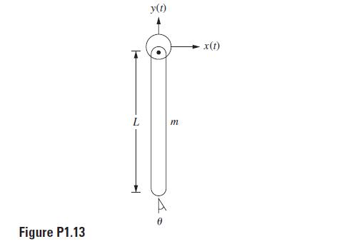
1.13 The differential equation governing the motion of the system of Figure P1.13 is
where x(t) and y(t) are known functions of time. Derive a linearized equation governing the motion of the system for small
2025 Cengage. All Rights Reserved. May not be scanned, copied or duplicated, or posted to a publicly accessible website, in whole or in part.
Solution
The differential equation is linearized by using the small angle assumption which implies sin ���� ≈ ���� and cos ���� ≈ 1. Using these approximations in the differential equation leads to the linearized approximation as
1.14 A chemical reaction that converts moles of a reactant A into moles of a substance B occurs in a continuously stirred tank reactor. The reaction is exothermic, and heat is given off during the reaction. The reactor is cooled by adding heat at a rate ���� to the reactor. The differential equations governing the concentration of the reactant CA and the temperature in the reactor T are
where V is the volume of the reactor, q is the flow rate of the reactant into the reactor, ���� is the heat of reaction, E is the activation energy of the reaction, R is the universal gas constant, a is a constant related to the rate of reaction, ���� is the mass density of the inlet stream, cp is the specific heat of the mixture, CAi is the concentration of the reactant in the inlet stream, and Ti is the temperature of the inlet stream. The steady-state conditions CAs and Ts are determined from Equations (a) and (b) by setting ���� �������� �������� = �������� �������� = 0
The reactor is operating at steady state when it is subject to a sudden change in the flow rate of the inlet stream defined so that the flow rate is
where qs is the flow rate at steady state and qp is the perturbation in the flow rate. The sudden change in flow rate leads to transient behavior in the reactor with time-dependent changes in reactant concentration and temperature defined by
Derive a set of linearized equations that could be solved to obtain the perturbations in reactant concentration and temperature.
Solution
The steady-state condition are obtained by setting the derivatives to zero in Equations (a) and (b) leading to
© 2025 Cengage. All Rights Reserved. May not be scanned, copied or duplicated, or posted to a publicly accessible website, in whole or in part.
Substitution of Equations (d) and (e)into Equations (a) and (b) leads to
The exponential terms are linearized by making a Taylor series expansion about �������� leading to
Use of Equation (j) in Equations (h) and (i) leads to
Equations (f) ad (g) are used to simplify Equations (k) and (l) to
Neglecting products of perturbation variables in Equations (m) and (n) leads to
1.15 The differential equation governing the transient temperature in a structure is
where cp is the specific heat of the material from which the structure is made, R is its thermal resistance, and T∞ is the ambient temperature of the surrounding medium. The specific heat of a material is a function of temperature. However, in many thermal problems the changes in temperature are small and the specific heat is not greatly affected. It is common to assume a constant value for cp, perhaps evaluated at T∞. Consider a situation in which the ambient temperature has a sudden large perturbation ����∞ (t) from its steady-state value of ����∞���� , resulting in a transient temperature in the structure defined by ���� = �������� + �������� (����). The temperature-dependent form of the specific heat for the structure is
© 2025 Cengage. All Rights Reserved. May not be scanned, copied or duplicated, or posted to a publicly accessible website, in whole or in part.
(a) Use binominal expansions to linearize Equation (b), assuming the perturbation temperature is small compared to the steady-state temperature. (b) Derive a linearized mathematical model for the perturbation temperature Solution
(a) Substituting the temperature expansion into Equation (b) leads to
Using the binominal expansion to linearize Equation (c) yields
(b) Substituting Equation (d) into Equation (a) gives
Terms such as �������� ���� �������� �������� are nonlinear and neglected compared to ������������ �������� . The steady-state condition is defined by ������������ �������� and �������� = ����∞ . These simplifications lead to
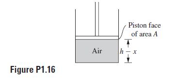
1.16 An air spring consists of a piston moving in a cylinder of compressed air. When the piston is in equilibrium, the height of the column of air is h and it exerts a pressure p0 on the face of the piston. The area of the face is A. When the piston moves a distance x downward, as illustrated in Figure P1.16, the air is further compressed. The process is assumed to be isentropic so that the air pressure is related to its density by
) where C is a constant and ���� is the ratio of specific heats. (a) Derive a relation between the force on the piston and the distance the piston moves into the column of air x. Hint: The mass of the air in the cylinder is constant. (b) Linearize the relationship of part (a) so that the force acting on the face of the piston is approximated as
Specify ���� .
= ����0 ���� + �������� (����)
Solution
(a) The mass of the air in the cylinder is constant and is calculated when the piston is in equilibrium as ���� = ����0 ����ℎ (���� ) where ����0 is the density of the air in equilibrium. Using Equation (a) in Equation (c) leads to
© 2025 Cengage. All Rights Reserved. May not be scanned, copied or duplicated, or posted to a publicly accessible website, in whole or in part.
where ����0 is the pressure in the cylinder when the piston is in equilibrium. At any instant the mass is calculated as
Equating Equation (e) to Equation (d) gives
The force on the piston is given by
(b) Equation (g) is rewritten as
Assuming ���� /ℎ≪ 1 a binomial expansion can be used on the right-hand side of Equation (h). Keeping only through the linear term in the binomial expansion leads to
From Equation (i) the stiffness is identified as
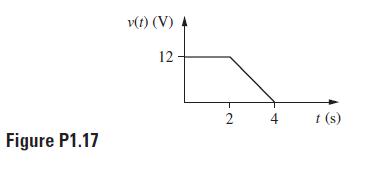
1.17 The time-dependent voltage of Figure P1.17 is supplied by a source in a series LRC circuit. Write a unified mathematical representation of the voltage provided by the source using unit step functions.
Solution
The superposition of the force is shown below
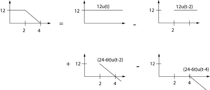
The mathematical representation is ���� (����) = 12[���� (����) ���� (���� 2)] + (24 6����)[���� (���� 2) ����(���� 4)] (����)
1.18 A mechanical system is subject to the time-dependent force shown in Figure P1.18. Develop a unified mathematical representation of the force using unit step functions.
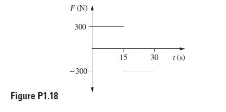
Solution
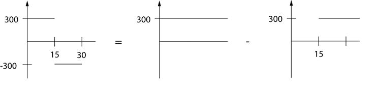
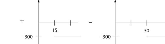
The superposition of the force is shown below
2025 Cengage. All Rights Reserved. May not be scanned, copied or duplicated, or posted to a publicly accessible website, in whole or in part.
The mathematical representation is ���� (����) = 300[���� (����) ���� (���� 15)] 300[���� (���� 15) ���� (���� 30)] (���� )
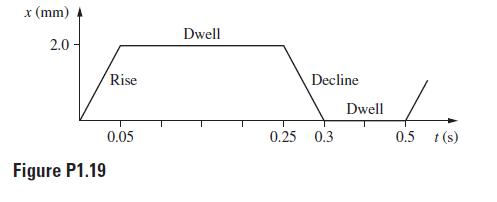
1.19 A cam and follower system has been designed to provide a periodic displacement to a valve in a mechanical system. Figure P1.19 illustrates the displacement provided over one period. (a) Use unit step functions to write a unified mathematical representation for the displacement over one period. (b) The displacement provided by the cam and follower system is periodic of period 0.5 s. Generalize the results of part (a) to provide a unified mathematical representation of the displacement for all time. Hint: Use an infinite series representation of the displacement with the index of summation representing one period.
Solution
The superposition of the cam displacement over one period is shown below
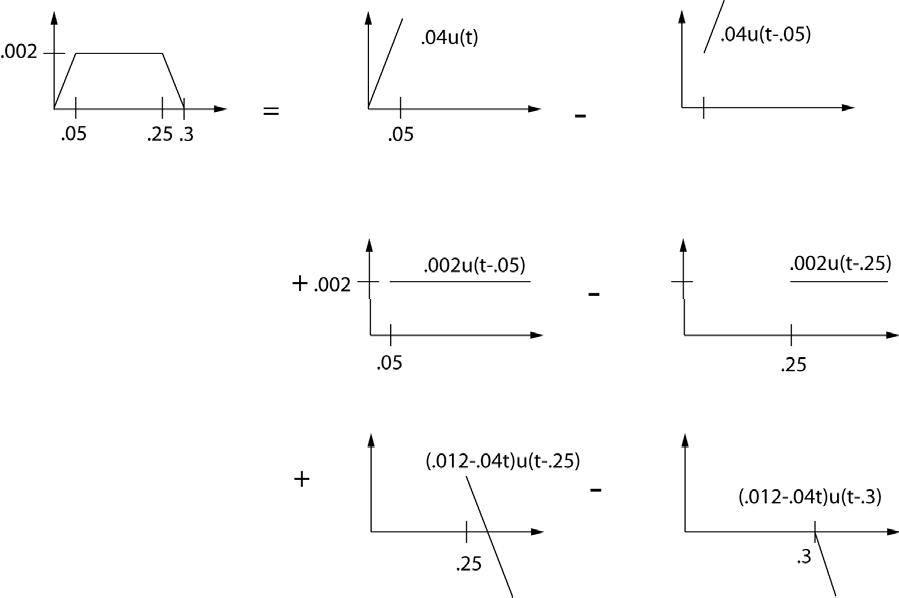
(a) The mathematical representation for the displacement over one period is ���� (����) = 0 04[���� (
) ����(
0 05)] + 0 002[
(
0 05) ���� (���� 0 25)] + (0 012 0.04
(b) The period of one cycle is 0.5 s. Thus, the displacement over the second cycle is obtained by replacing ���� in Equation (a) by ���� + 0.5. The displacement over the kth cycle is obtained by
© 2025 Cengage. All Rights Reserved. May not be scanned, copied or duplicated, or posted to a publicly accessible website, in whole or in part.
replacing ���� in Equation (a) by ���� + (����− 1)0.5. The total displacement if obtained by summing over each cycle
) =
1.20 A particle of mass 4 kg is at rest when it is subject to an impulsive force that imparts a total impulse of 12 N∙s to the mass. Knowing that Newton’s second law can be written as ���� = ���� �������� �������� , determine the velocity of the particle after application of the impulse.
Solution
Integration of Newton’s second law with respect to time leads to the principle of impulse and momentum ���� = � ���� ����2 ����1 �������� �������� �������� =
(
−����1 ) (���� )
where ���� is the total impulse applied over the period. The 12 N∙s impulse if applied instantaneously to the 4-kg particle which is initially at rest. Application of the Principle of impulse and momentum leads to 12 =4����2 ⟹����2 =3 m s (����)
1.21 No current is flowing through a circuit when it is subject to an impulsive voltage such that the total impulse is 20 V∙s. Knowing that the relation between voltage and current in an inductor is ���� = ���� �������� �������� , where L = 0.4 H is the inductance, determine the current through the inductor immediately after application of the impulse.
Solution
Integration of the relation between voltage and current in an inductor leads to � ���� �������� ���� 0 = ����(����2 −����1 ) (���� )
The initial current is zero. Solving Equation (a) for the current after the impulse occurs gives 20 =0.4����2 ⟹����2 = 50 A (����)
1.22 A machine is subject to three impulses: an impulse of magnitude 100 N s applied at ���� = 0, an impulse of magnitude 150 N∙s applied at ���� = 2.5 s, and an impulse of magnitude 50 N∙s applied at ���� = 3 8 s. What is the mathematical formulation for the force applied to the machine?
Solution
The mathematical representation of the force is ���� (����) = 100���� (����)
1.23 The steady-state current in a series LRC circuit due to a sinusoidal voltage source is ���� (����) = ����0 ���� ���� 1 �(���� 2 −�������� 2 )2 + (2�������� �������� )2 sin
2 2�������� ��������
(���� ) where the circuit’s natural frequency is �������� = 1 √�������� damping ratio is ���� = ���� 2 ����� ���� . Write a MATLAB M-file that does the following: (a) inputs the values of resistance (R) in ohms, capacitance (C) in farads, inductance (L) in henrys, input frequency (���� ) in rad/s, and input amplitude (V0) in volts; (b) evaluates i(t) for 200 discrete values of t in the interval 0 ≤ t ≤ 10���� ���� ; and (c) plots the response with an annotated graph.
© 2025 Cengage. All Rights Reserved. May not be scanned, copied or duplicated, or posted to a publicly accessible website, in whole or in part.
Solution
The MATLAB file Problem1_23 which determines the steady-state response of a series LRC circuit is listed below
% Problem1_23.m
% Steady-state response of series LRC circuit
clear
disp('Steady-state response of series LRC circuit')
% Input parameters
disp('Input resistance in ohms')
R=input('>> ')
disp('Input capacitance in farads')
C=input('>>')
disp('Input inductance in henrys')
L=input('>> ')
disp('Input source frequency in r/s') om=input('>> ')
disp('Input source amplitude in V')
V0=input('>> ')
% Calculates parameters
disp('Natural frequency in r/s =')
omn=1/(L*C)^0.5
disp('Dimensionless damping ratio =')
zeta=R/2*(C/L)^0.5
disp('Phase angle in rad=')
C1=om^2-omn^2;
C2=2*zeta*om*omn; phi=atan2(C1,C2)
disp('Steady-state amplitude in A =')
C3=V0*om/L;
C4=1/(C1^2+C2^2)^0.5;
I=C3*C4
tf=10*pi/om; dt=tf/200; for k=1:201
t(k)=(k-1)*dt; i(k)=I*sin(om*t(k)+phi); end
plot(t,i)
xlabel('t (s)')
ylabel('i (A)')
title('Steady-state response of series LRC circuit')
str1=['R=',num2str(R),' \Omega'];
str2=['C=',num2str(C),' F'];
str3=['L=',num2str(L),' H'];
str4=['\omega=',num2str(om),' r/s'];
str5=['V_0=',num2str(V0),' V'];
text(0.9*tf,I,str1)
text(0.9*tf,0.8*I,str2)
text(0.9*tf,0.6*I,str3)
text(0.9*tf,0.4*I,str4)
text(0.9*tf,0.2*I,str5)
© 2025 Cengage. All Rights Reserved. May not be scanned, copied or duplicated, or posted to a publicly accessible website, in whole or in part.
The MATLAB workspace from a sample execution of Problem1_23.m is >> Problem1_23
Steady-state response of series LRC circuit
Input resistance in ohms >> 100
R = 100
Input capacitance in farads >>0.2e-6
C = 2.0000e-007
Input inductance in henrys >> 0.5
L = 0.5000
Input source frequency in r/s >> 2000
om = 2000
Input source amplitude in V >> 120
V0 = 120
Natural freqeuncy in r/s = omn = 3.1623e+003
Dimensionless damping ratio = zeta = 0.0316
Phase angle in rad= phi = -1.5042
Steady-state amplitude in A = I = 0.0798
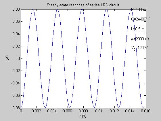
The resulting steady-state plot is
1.24 Write a MATLAB M-file that (a) inputs the elements of two 5x5 matrices A and B; (b) calculates A+ B; (c) calculates AB; (d) calculates A-1; (e) calculates det(A); and (f) determines the eigenvalues and eigenvectors of A (see Appendix B) using the MATLAB function eigs. Solution
The MATALB file Prolbem1_24.m is listed below
% Problem1_24.m
%(a) Input two five by five matrices
disp('Please input matrix A by row') for i=1:5 for j=1:5
str={['Enter A(',num2str(i),num2str(j),')']};
disp(str)
A(i,j)=input('>> '); end end
disp('Please input matrix B by row') for i=1:5 for j=1:5
str={['Enter B(',num2str(i),num2str(j),')']};
disp(str)
B(i,j)=input('>> '); end end
A B
% (b) =A+B
C=A+B
% (c) D=A*B
D=A*B
% (d) det(A)
detA=det(A)
% eigenvalues and eigenvectors of A
[x,Y]=eigs(A); disp('Eigenvalues of A')
Y
disp('Matrix of eigenvalues of A') x
A sample output from execution of the file is shown below >> clear >> Problem1_24
Please input matrix A by row
'Enter A(11)' >> 1
'Enter A(12)' >> 0
'Enter A(13)' >> 12
'Enter A(14)' >> -1
'Enter A(15)' >> 21
'Enter A(21)' >> 14
'Enter A(22)' >> -3
'Enter A(23)' >> 2
'Enter A(24)' >> 0
'Enter A(25)' >> -22
'Enter A(31)' >> 11
'Enter A(32)' >> 12
'Enter A(33)' >> 10
'Enter A(34)' >> -4
'Enter A(35)' >> 12
'Enter A(41)' >> 10
2025 Cengage. All Rights Reserved. May not be scanned, copied or duplicated, or posted to a publicly accessible website, in whole or in part.
'Enter A(42)'
>> 11
'Enter A(43)'
>> 18
'Enter A(44)'
>> 12
'Enter A(45)'
>> 21
'Enter A(51)' >> 10
'Enter A(52)' >> 11
'Enter A(53)'
>> 31
'Enter A(54)'
>> 21
'Enter A(55)' >> 11
Please input matrix B by 'Enter B(11)'
>> 21
'Enter B(12)'
>> -21
'Enter B(13)'
>> 21
'Enter B(14)'
>> 10
'Enter B(15)' >> 9
'Enter B(21)'
>> 8
'Enter B(22)'
>> 2
'Enter B(23)'
>> 2
2025 Cengage. All Rights Reserved. May not be scanned, copied or duplicated, or posted to a publicly accessible website, in whole or in part.
'Enter B(24)'
>> 4
'Enter B(25)'
>> -5
'Enter B(31)'
>> 16
'Enter B(32)'
>> 12
'Enter B(33)'
>> 11
'Enter B(34)'
>> 18
'Enter B(35)' >> 11
'Enter B(41)'
>> 21
'Enter B(42)'
>> 32
'Enter B(43)'
>> 14
'Enter B(44)'
>> 19
'Enter B(45)'
>> 12
'Enter B(51)'
>> 12
'Enter B(52)'
>> 9
'Enter B(53)'
>> -5
'Enter B(54)'
>> 13
'Enter B(55)'
>> 21
12 10 -4 12
10 11 18 12 21
10 11 31 21 11 B = 21 -21 21 10 9
8 2 2 4 -5 16 12 11 18 11 21 32 14 19 12
12 9 -5 13 21 C =
1.25 The function
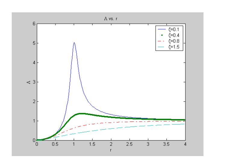
) is used in the analysis of the steady-state response of certain mechanical systems. Write a MATLAB Mfile that plots, on the same axes, L vs. r for five different values of ���� . The plot should be annotated Solution
(1
)
+ (2
A MATLAB file to calculate and plot LAMBD (r, ���� ) is given below
% Plots the function LAMBDA(r,zeta) as a function of r for several values of % zeta
% Specify four values of zeta: zeta1=0.1; zeta2=0.4; zeta3=0.8; zeta4=1.5;
% Define values of r for calculations for i=1:400
r(i)=(i-1)*.01;
% Calculate function
LAMBDA1(i)=r(i)^2/((1-r(i)^2)^2+(2*zeta1*r(i))^2)^0.5; LAMBDA2(i)=r(i)^2/((1-r(i)^2)^2+(2*zeta2*r(i))^2)^0.5; LAMBDA3(i)=r(i)^2/((1-r(i)^2)^2+(2*zeta3*r(i))^2)^0.5; LAMBDA4(i)=r(i)^2/((1-r(i)^2)^2+(2*zeta4*r(i))^2)^0.5; end plot(r,LAMBDA1,'-',r,LAMBDA2,'.',r,LAMBDA3,'-.',r,LAMBDA4,' ') xlabel('r') ylabel('\Lambda')
str1=['\zeta=',num2str(zeta1)];
str2=['\zeta=',num2str(zeta2)];
str3=['\zeta=',num2str(zeta3)];
str4=['\zeta=',num2str(zeta4)]; legend(str1,str2,str3,str4) title('\Lambda vs. r')
The resulting output from execution of the .m file is the following plot
© 2025 Cengage. All Rights Reserved. May not be scanned, copied or duplicated, or posted to a publicly accessible website, in whole or in part.
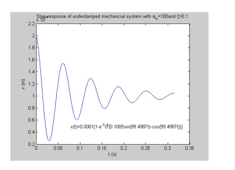
1.26 The step response of an underdamped mechanical system of natural frequency �������� and damping ratio���� is
) = 1
Where �������� = �������� �1 −���� 2 . Write a MATLAB M-file that (a) inputs the values of natural frequency and damping ratio and (b) evaluates and plots the step response on an annotated graph. The response should be evaluated for at least five cycles, ���� =5 � 2����
Solution
The MATALB .m file Problem1_26 which determines and plots the step response of an underdamped mechanical system is shown below.
% Problem1_26.m
% Step response of an underdamped mechanical system
% Input natural frequency and damping ratio clear disp('Step response of underdamped mechanical system')
© 2025 Cengage. All Rights Reserved. May not be scanned, copied or duplicated, or posted to a publicly accessible website, in whole or in part.
disp('Please input natural frequency in r/s')
om=input('>> ')
disp('Please input the dimensionless damping ratio')
zeta=input('>> ')
% Damped natural frequency
omd=om*(1-zeta^2)^0.5; C1=zeta*om/omd; C2=1/om^2; C3=zeta*om; tf=10*pi/omd; dt=tf/500; for i=1:501
t(i)=(i-1)*dt;
x(i)=C2*(1-exp(-C3*t(i))*(C1*sin(omd*t(i))-cos(omd*t(i)))); end
plot(t,x)
xlabel('t (s)')
ylabel('x (m)')
str1=['Step response of underdamped mechanical system with \omega_n=',num2str(om),'and \zeta=',num2str(zeta)]
title(str1)
str2=['x(t)=',num2str(C2),'[1-e^-^',num2str(C3),'^t(',num2str(C1),'sin(',num2str(omd),'t)cos(',num2str(omd),'t))]']
text(tf/4,C2/2,str2)
Output from execution of Problem1_26 follows >> Problem1_26
Step response of underdamped mechanical system
Please input natural frequency in r/s >> 100 om = 100
Please input the dimensionless damping ratio >> 0.1
zeta = 0.1000
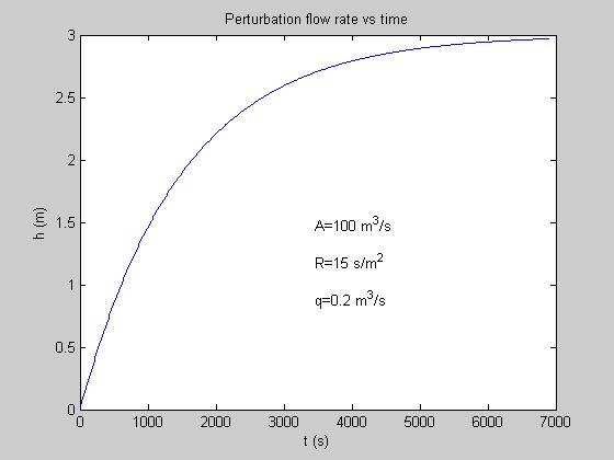
1.27 The perturbation in the liquid level in a tank of area A and hydraulic resistance R due to a flow rate perturbation q is
ℎ(����) = �������� �1 ���� ����/(��������) � (���� )
(a) If A is in square meters (m2) and t is measured in seconds (s), what are the units of R? (b) It is noted that lim ����→∞ ℎ(����) = �������� , which is its steady-state value. Write a MATLAB program that, given q, R, and A, calculates an h(t) until it is within 0.1% of the steady-state value. (c) Use the MATLAB program to plot h(t).
Solution
(a) Since the argument of a transcendental function must be dimensionless the dimensions of the product of resistance and area must be time. Thus the dimensions of resistance must be � ���� ����2 �
(b) Note that the steady-state value of the liquid-level perturbation is qR. The MATLAB file Problem1_27.m which calculates and plots h(t) from t=0 until h is within 1 percent of its steady-state value is given below
© 2025 Cengage. All Rights Reserved. May not be scanned, copied or duplicated, or posted to a publicly accessible website, in whole or in part.
disp('Please enter resistance in s/m^2 ')
R=input('>> ')
% Final value of h
hf=0.99*q*R;
dt=0.01*R*A; h1=0; h(1)=0; t(1)=0; i=1; while h1<hf i=i+1; t(i)=t(i-1)+dt; h(i)=q*R*(1-exp(-t(i)/(R*A))); h1=h(i); end plot(t,h)
xlabel('t (s)')
ylabel('h (m)')
title('Perturbation flow rate vs time')
str1=['A=',num2str(A),' m^3/s']
str2=['R=',num2str(R),' s/m^2']
str3=['q=',num2str(q),' m^3/s']
text(0.5*t(i),0.5*h(i),str1);
text(0.5*t(i),0.4*h(i),str2);
text(0.5*t(i),0.3*h(i),str3);
Sample output from execution of Problem1_27.m is given below
>> Please enter tank area in m^2 >> 100 A = 100
Please enter flow rate in m^3/s >> 0.2
q = 0.2000
Please enter resistance in s/m^2 >> 15
R = 15
str1 =
A=100 m^3/s str2 = R=15 s/m^2
2025 Cengage. All Rights Reserved. May not be scanned, copied or duplicated, or posted to a publicly accessible website, in whole or in part.
m^3/s