Solutions Manual for Mathematical Statistics with Applications 8th Edition by Wackerly, Chen
ISBN: 9798214013435
Solution and Answer Guide: Dennis D. Wackerly, Wackerly, 8e, ©2027, 9798214013435; Chapter 1: What is Statistics?

ISBN: 9798214013435
Solution and Answer Guide: Dennis D. Wackerly, Wackerly, 8e, ©2027, 9798214013435; Chapter 1: What is Statistics?
D ENNIS D. W ACKERLY , W ACKERLY , 8 E , © 2027 , 9798214 01 3435 ; C HAPTER 1: W HAT IS S TATISTICS ?
1.1 Answers may vary
1.
a. Population of interest: all U.S. citizens who are members of Generation X (as defined by the study commonly birth years ~1965–1980)
Inferential objective: Estimate a population proportion: the proportion of Gen X U.S. citizens interested in starting their own business.
How to collect a sample: Use a national survey with a probability-based sampling method (e.g., stratified random sampling by region, gender, etc.). Screen respondents to confirm Gen X and U.S. citizenship, then ask the interest question.
b. Population of interest: all healthy adults in the United States
Inferential objective: Estimate the population mean body temperature (and compare to 98.6°F informally or via a confidence interval).
How to collect a sample: Select a random sample of adults (possibly stratified by age/sex/region). Measure temperature using a standardized method (same type of thermometer, same body location, similar conditions/time of day), and exclude those who are ill.
c. Population of interest: all single-family dwelling units in the city
Inferential objective: Estimate the population’s mean weekly water consumption. How to collect a sample: Take a simple random sample (or stratified by neighborhood/size) of single-family addresses from utility records and use meter data for a defined week (or average across several weeks to reduce week-to-week variation).
d. Population of interest: all automobile tires manufactured by that company during the current production year
Inferential objective: Estimate the population proportion with unsafe tread.
How to collect a sample: Use quality-control sampling from production lots: randomly sample tires throughout the year (stratify by plant, line, tire model, month). Measure tread depth and classify “unsafe” by a defined standard.
2.
Solution and Answer Guide: Dennis D. Wackerly, Wackerly, 8e, ©2027, 9798214013435; Chapter 1: What is Statistics?
e. Population of interest: all adult residents of the state
Inferential objective: Determine whether the population proportion favoring unicameral legislature is greater than 0.50 (a majority). (This is a hypothesis test about a proportion.)
How to collect a sample: Conduct a statewide random poll (stratified by region/urban-rural, etc.). Use multiple contact methods (phone/text/online) and weight appropriately to match known demographics.
f. Population of interest: patients with the disease who become recurrence-free after treatment (often defined more precisely as patients meeting eligibility criteria in a target health system or in the U.S.).
Inferential objective: Estimate the mean (or typical) time to recurrence; in practice this is often a survival/time-to-event objective.
How to collect a sample: Use a cohort study: enroll a sample of eligible patients and follow them over time, recording recurrence times. This usually requires handling censoring (patients lost to follow-up or recurrence not observed by study end).
g. Population of interest: all transistors of that specific type (from the relevant production process/time period).
Inferential objective: Test whether the population mean lifetime is greater than 500 hours (hypothesis test on a mean).
How to collect a sample: Randomly sample transistors from production (possibly stratified by batch/line), then run a life test under standardized operating conditions until failure (or use accelerated life testing, with appropriate statistical adjustment).
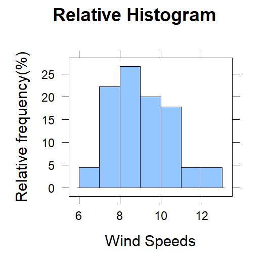
b. Yes, it is quite windy there.
c. 9/45, or approx. 20%
d. It is not especially windy in the overall sample.
5.
Solution and Answer Guide: Dennis D. Wackerly, Wackerly, 8e, ©2027, 9798214013435; Chapter 1: What is Statistics?
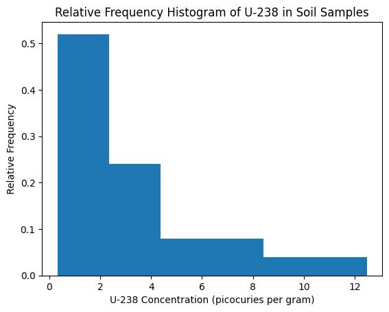
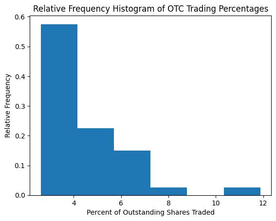
b. 18/40 45% =
c. 29/40 72.5% =
a. The 2.45 –2.65 and 2.65 –2.85 GPA categories have the tallest bars, so these intervals are associated with the largest proportion of students.
b. The proportion in each category is: 6/30 0.20. = So, 20% of the students fall in each of these two categories.
c. The proportion of students that has GPAs less than 2.65 is 3/30 3/30 3/30 6/30 0.50 +++= or 50%.
6.
7.
8.
9.
Solution and Answer Guide: Dennis D. Wackerly, Wackerly, 8e, ©2027, 9798214013435; Chapter 1: What is Statistics?
a. The modal category is 2 (quarts of milk). About 36% (9 people) of the 25 are in this category.
b. 0.20.120.040.36 ++=
c. Note that 8% purchased 0 while 4% purchased 5. Thus, 1–.08–.04.88 = purchased between 1 and 4 quarts.
a. The histogram is bimodal.
b. Yes. The distribution has two peaks (2 modes).
c. The two peaks likely result from combining male and female height data, which have different average heights.
a.
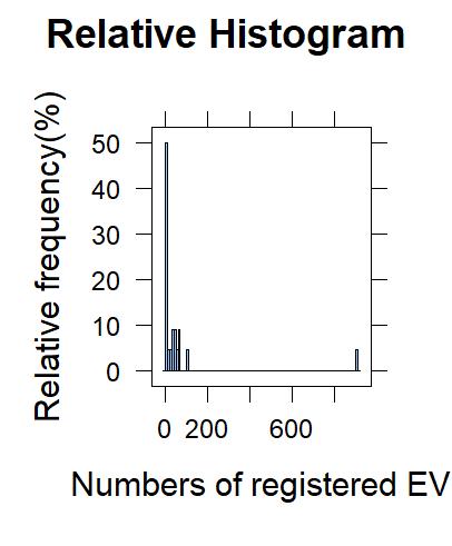
b. The data appears to have outliers. Two states in the West region have sample values much higher than the rest.
a. 9.7121 σ =− , 14.3121 σ =+ . About 68% lie within 1 µσ ± .
b. 7.4122σ =− , 16.6122σ =+ . About 95% lie within 2 µσ ± .
c. From the empirical rule, 68% within 1 µσ ± and an additional 13.5% fall between 1 µσ + and 2 µσ + . So, 0.680.1350.815 += or 81.5%
d. 5.1123σ =− , 18.9123σ =+ . About 99.7% lie within 3 µσ ± . So, 1–0.9970.003 = or 0.3%.
Solution and Answer Guide: Dennis D. Wackerly, Wackerly, 8e, ©2027, 9798214013435; Chapter 1: What is Statistics?
10.
a. 14–173. =−
b. Since 68% lie within 1 standard deviation of the mean, 32% should lie outside. By symmetry, 16% should lie below 1 standard deviation from the mean.
c. If normally distributed, approximately 16% of people would spend less than –3 hours on the internet. Since this doesn’t make sense, the population is not normal.
11.
So that
Writing
12.
So that
Dividing both sides by 1 n and summing from 1 to n , we get
Solution and Answer Guide: Dennis D. Wackerly, Wackerly, 8e, ©2027, 9798214013435; Chapter 1: What is Statistics?
14.
a. 25 1 80.63 i i y = ∑ and 25 2 1
b.
15.
(2.516, 6.258)
16.
a. Without the extreme value, 4.19 y = and 1.44. s =
b. These counts compare more favorably:
2.75, 5.63 25
2 1.31, 7.07 36
3 –0.13, 8.51 39 39
17.
For 1.2: min6.0, = max12.3 r ange6.3. = = So, range/46.3/41.575. == 1.447, s = which is 0.128 lower than the estimate. For 1.3: min0.32, = max12.48 r ange12.16. = = So, range/412.16/43.04. == 3.167, s = which is 0.127 higher than the estimate.
For 1.4: min2.61, max11.88 r ange9.27. = = = So, range/49.27/42.3175. == 1.871, s = which is 0.446 lower than the estimate.
Solution and Answer Guide: Dennis D. Wackerly, Wackerly, 8e, ©2027, 9798214013435; Chapter 1: What is Statistics?
18.
min200, max800range600. ==⇒= From 17, 600 150. 44 range s ≈==
19.
If chloroform amounts were normally distributed, then by the empirical rule, about 95% of the observations would fall within
µσ±=±=±=−2342533410672, 140.
Since chloroform concentration cannot be negative, the distribution of chloroform amounts cannot be normal.
20.
15,50014,20011. =+=+σµσ About 68% of values lie within 1. ± µσ So, 32% lie outside this interval. By symmetry, half of that or 16% lie above 115,500.µσ+=
21.
2022–11. ==−σµσ About 68% of values lie within 1. ± µσ So, 32% lie outside. By symmetry, 16% lie below 1.µσ Thus, 1–0.160.84 = or 84% should have weight gains in excess of 20 pounds. Hence, the sample information does not contradict the manufacturer’s claim.
22.
Probability is the measurement of uncertainty for statistical inference.
23.
No. You can only say that 40% is an estimate of the true population of smokers, since this value comes from a sample of 50 patients, and is subject to sampling error. Different random samples would likely produce different results.
24.
25.
a. 302511. =+=+σµσ So, by the empirical rule, 16% lie above 1.µσ +
b. 152, 454. =−=+µσµσ By the empirical rule, 95% of the data fall within 2.µσ + So, by symmetry, 2.5% fall below 2.µσ Also, about 0.15% falls beyond 3.µσ + So, beyond µσ + 4 is approximately 0.
c. 902513. σ =+ That’s extremely far from the mean. So, the probability is approximately 0. Thus, it is very unlikely that a commercial will last longer than 1.5 minutes or 90 seconds.
Solution and Answer Guide: Dennis D. Wackerly, Wackerly, 8e, ©2027, 9798214013435; Chapter 1: What is Statistics?
26.
a. ( ) 188.22105.6/420.66 −=
b.
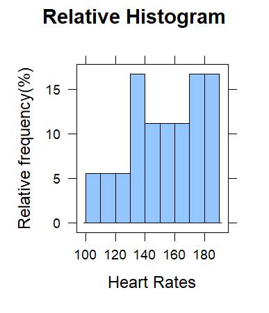
c. Using R, we have that 152.76 y = and 25.16. s =
d.
27.
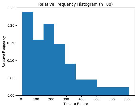
a. Rangemax–min716–8708. = == So, 708 177 44 Range s ≈== b. c. = 210.80 y , = 162.17 s
Solution and Answer Guide: Dennis D. Wackerly, Wackerly, 8e, ©2027, 9798214013435; Chapter 1: What is Statistics?
1 (48.62, 372.97) 63
2 (-113.55, 535.14) 82
3 (-275.72, 697.31) 87
28. For Ex. 1.12, 3/1.212.48. = For Ex. 1.26, 82.62/25.163.28. = For Ex. 1.27, 708/162.174.37. = The ratio increases as the sample size increases.
29.
72, 8, 340ysn=== 64721, 80721. ss=−=+ So, by the empirical rule, () 0.68340231 = in the interval 64 to 80. 56722, 88722. ss=−=+ So, by the empirical rule, () 0.95340323 = in the interval 56 to 88.
30. 13mg/L is 1 standard deviation below the mean, so 16%.
31.
a. () =−=−µσ 2.983.0020.012 , () =+=+µσ 3.023.0020.012
So, bearings that fail are those outside the interval: µσ ± 2 . By the empirical rule, about 95% of observations fall within 2.µσ + So, 5% fall outside the interval.
b. The bearing diameters are approximately normally distributed.
32.
If μ10 = and σ1.2, = we expect 34% to be between 10 and 101.211.2. += Also, approximately 95%/247.5% = will lie between 10 and 12.4. So, approximately 47.5%–34%13.5% = should lie between 11 and 13.
33.
() 40602102. =−=−µσ By the empirical rule, about 95% of values are within 2.µσ ± This leaves 5% outside this interval. By symmetry, the probability of a yield less than 40 is approximately 0.025 or 2.5%. This could raise suspicion of an abnormality. The assumptions are that daily yield is approximately normally distributed and the mean and variance are stable over time.
34.
Let m be the number of i such that i yyks −≥ For each of the m observations outside the interval, we have
Solution and Answer Guide: Dennis D. Wackerly, Wackerly, 8e, ©2027, 9798214013435; Chapter 1: What is Statistics?
()() 22 22 . i yyksks −≥= For the remaining nm observations, ()2 0. i yy−≥ Therefore,
()
() = = ∑∑−≥⇒=−≥ 22 222 22 11 11 11 nn ii ii yymkss yymks nn
35.
Thus,
≥⇒≤ 2 2 1 1 1 mkn m n k
So, the number of measurements inside the interval is at least −≥−⇒≥− 22 11 1 nnmn nmn n k nk
Now, since ≤ 1 1 n n ,
−≥− 22 11 11 n nkk
Thus, the fraction of measurements inside the interval yks to + yks is at least 2 1 1 k
Using Chebyshev’s inequality, we have that
−≥⇒≥ 2 1 10.752 k k .
Then, for = 2 k , with = 5.5 y and = 2.5 s , we have () ±=±=± 25.522.55.55ys
So, at least 75% of the days absent count must fall in the interval (0.5, 10.5).
36.
The point 13 is 13–5.57.5 = units above the mean, or 7.5/2.53 = standard deviations above the mean. By Chebyshev’s Inequality, at least 1–1/328/9 = will lie within 3 standard deviations of the mean. Thus, at most 1/9 of the values will exceed 13.
37.
a. ≈== 172108 16 44 Range s
b. ==136.07, 17.10ys
c. At least −≥⇒= 2 1 10.752 k k
So, () () =−=−==+=+= 2136.07217.10101.86, 2136.07217.10170.27ays bys
d. The number of readings in the interval (101.86, 170.27) is 14. And = 14 0.9333 15 or 93.3%. So, yes, the inequality worked.
or
38. a.
Solution and Answer Guide: Dennis D. Wackerly, Wackerly, 8e, ©2027, 9798214013435; Chapter 1: What is Statistics?
b. With = ∑
and
we have
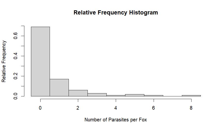
c. Within 2 standard deviations: 95, within 3 standard deviations: 96. The calculations agree with Chebyshev’s Inequality.
39.
If the lead content readings were normally distributed, then by the empirical rule about 95% of the values would lie within the interval ()( ) µσ±=±=−20.02720.120.213, 0.267 . Since this interval includes negative numbers and lead concentrations must be nonnegative, the distribution of lead readings cannot be normal.
40. By Chebyshev’s inequality, at least ¾ 75% = lie between ()0, 140, at least 8/9 lie between ()0, 193, and at least 15/16 lie between ()0, 246. Note: the lower bounds are all truncated to 0 since the measurement cannot be negative.