Solutions Manual for Making Sense of Behavioral Statistics v1 1st Edition by Lorch
ISBN: 9781453341483

ISBN: 9781453341483
Appendix F presents grading information from a course and asks several questions about performance in the course. Analyses relevant to each of the questions are planned out, and their rationale is explained, then the analyses are performed and interpreted. Most of the procedures studied for correlation and regression are applied.
A single (hypothetical) dataset is presented for the end-of-chapter exercises and several questions are asked about the data. The questions are designed to give students practice with most of the correlation and regression procedures they have learned.
1. For the males: by.x = (0.43)(15,036/6.2) = 1042.82 ay.x = 101,642 – (1042.82)(19.4) = 81,411.292 Predicted income = 81,411.292 + (1042.82)(Years)
2. For females: by.x – (0.58)( 10,793/4.1) = 1526.82 ay.x = 92,789 – (1526.82)(12.5) = 73,703.75 Predicted income = 73,703.75 + (1526.82)(Years)
3. t = ( 101,642 – 92,789 ) √[ ( 1950 ) ( 15,0362 )+( 808 ) ( 10,7932 ) 1950 +808 ][ 1 1951 + 1 809 ]
( 193,974,444.2 ) (.0017489 )
For (1950 + 808) = 2758 df, tcrit = Zcrit = 1.96 for alpha = 0.05, nondirectional test (although you could easily argue for a directional test). The observed t-value of 15.1997 greatly exceeds 1.96 so our conclusion is that male faculty have higher incomes than female faculty.
4. t = ( 19.4 12.5 ) √[ ( 1950 ) ( 6.22 )+( 808 ) ( 4.12 ) 1950 + 808 ][ 1 1950 + 1 808 ] = 6.9 √ ( 32.10315 ) .0017489 ¿ ¿= 6.9 0.23695 =29.12
The computed t of 29.12 exceeds the critical value of 1.96, so we can conclude that male faculty have, on average, more years on the faculty.
5. Converting rxy to ZF, the ZF for males is 0.4599 and the ZF for females is 0.6625.
Z = (0.4599 – 0.6625)/√( 1 1948 )+( 1 806 ) = –0.2026/0.0239 = -8.477
The observed Z-value of -8.477 exceeds the critical value of ±1.96 for alpha = 0.05 so we may conclude that the correlation between Income and Years is greater for female faculty than for male faculty.
6. We need to compute SEb1 – b2, which is best approached by computing intermediate results and assembling them:
For males: sy.x 2 = (1 – 0.432)(150362) = 184,278,864.4; SSx = (1950)(6.22) = 74,958
For females: sy.x 2 = (1 – 0.582)(10,7932) = 77,302,000.2; SSx = (808)(4.12) = 13,582.48 SE = √[ ( 1949 ) ( 184,278,864.4 )+ ( 807 ) ( 77,302,000.2 ) ( 1949 +807 ) ]( 1 74,958 + 1 13,582.48 ) = 115.333
t = (1042.82 - 1526.82)/115.333 = –4.197
For df = (1949 + 807) = 2756, tcrit for a nondirectional test at alpha = 0.05 is 1.96
The computed t-value exceeds –1.96 so we may conclude that the slope of the regression line relating Income to Years is greater for female faculty than for male faculty.
7. Male faculty have been employed for longer and make more money, on average, than female faculty at U.S. colleges and universities. For both males and females, there is a relatively high positive correlation between income and how long a faculty member has been employed at a school. However, the strength and description of the relationship between income and length of employment differs for men and women. There is a stronger correlation for females than males, and the slope of the regression line is greater for females.
Do these findings demonstrate a sex bias? The large difference in incomes for men versus women suggest a bias, although the nature of the bias is not immediately obvious from that simple difference. If we take the definition of bias as unequal pay for equal work, the difference in incomes alone is ambiguous. The finding of a large difference in length of employment also suggests a bias in the form of women finding it more difficult to be hired in the first place. We know that throughout much of the history of higher education, women had a much more difficult time being (a) accepted into graduate and professional schools than (b) finding employment at top colleges and universities. The finding of a substantial difference in length of employment for men versus women is consistent with this. Further, it explains—at least partially—the difference in incomes; that is, given a strong
relationship between income and length of employment, the fact that men have been employed longer than women account for at least some of their higher income. To the extent that the difference in years of employment is responsible for the income gap, the income gap should lessen and eventually disappear over time as any sex bias in hiring is eliminated.
The finding of a stronger relationship between Income and Years for women than men is difficult to interpret. It could simply reflect the fact that women have not been employed for as long as men, on average. A major determinant of income is the academic rank of a faculty member. For the first five or six years a faculty member is employed, they are untenured and at the rank of Assistant Professor. If a faculty member earns tenure, they continue on to the faculty and are promoted to the rank of Associate Professor around their sixth year. A substantial salary increase happens at that point. Around year 12, a faculty member will usually be considered for promotion to Full Professor. If promoted, there is another substantial salary increase. However, not all faculty members earn promotion to Full and, instead, remain at the associate level, perhaps for the remainder of their careers. So faculty who are employed beyond 12 years consist of highly-paid full professors and lesswell-paid associate professors; that is, the correlation between Income and Years breaks down somewhat for the most senior faculty members. Because there are many more longserving males than females, this may be the reason for the lower correlation and smaller slope for males than for females. (This is much more than you would be expected to know about faculty salary structure! I included the discussion just because there were correlation and slope differences between males and females that would likely be puzzling for a student.)

Robert F. Lorch, Jr.

Published by:
FlatWorld ©2024 by FlatWorld. All rights reserved. Your use of this work is subject to the license agreement available on our website at www.Flatworld.com/terms.
No part of this work may be used, modified, or reproduced in any form by any means except as expressly permitted under the licensing agreement.

• Learn how to study statistics.
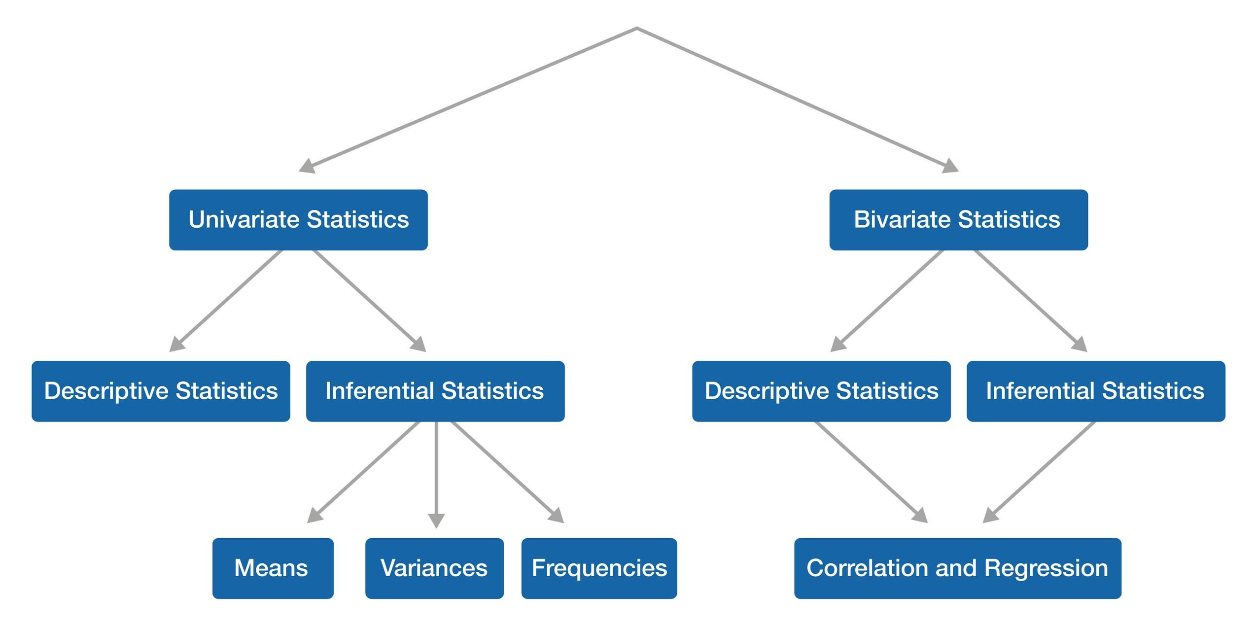
• Preview major topics in the book and their organization.
• Introduce a context for the first topic in the book, descriptive statistics.
Always aim for understanding!
Be patient
Study the textbook (don’t just read it)
Think as you read
Use the learning aids available in the chapters
Do the problems!
Learn the language of statistics
Use your resources
Research in the behavioral sciences usually involves the collection of many observations that are tabulated in some organized way, often on a spreadsheet.
The first step in making sense of a dataset is to describe the results in systematic ways.
One category of descriptive statistics is methods for capturing trends across the entire dataset by either
Constructing tables that organize the observations into meaningful categories and measure the observations in some way (e.g., simply count how many observations fall in each category) or
Drawing graphs that organize observations into categories
A second category of descriptive statistics includes measures of important characteristics of the dataset, such as Measures of a typical observation in a dataset
Measures of how much observations differ from one another
Student evaluations are solicited for every course at the end of each semester. In a course like introductory psychology, there may be 2,000 ratings compiled on each of the many questions in the survey. One question on the survey asks students to indicate their expected grade for the course. What would you like to know about students’ responses to this question?
You probably would like to see the entire distribution of responses to the question in a table or graph. How would you tabulate the observations? What would your categories be?
You might want to summarize the typical expected grade somehow. What might you select as a measure of the “typical” grade?
You might want to summarize the amount of variation in expected grades somehow. What might you select as a measure of variation?
Another question on the survey might be “What is your GPA in your college courses?” with students asked to type their answer to 2 decimal places.
How would you tabulate these observations into categories for presentation in a table or graph? How is this process more complicated than the tabulation of expected grades in the previous example?
How might you summarize the “typical” GPA? Would you choose the same measure that you selected for expected grades?
How might you summarize the amount of variability in GPAs? Again, would you do the same thing that you did for expected grades?
You are already familiar with many of the topics we will cover in our study of descriptive statistics.
Pay close attention to the “when?” and “why?” of the procedures we study.
Chapter 2 covers procedures for tabling and graphing entire distributions of observations
Chapter 3 covers statistics for summarizing the “typical” observation in a dataset, the amount of variation in observations in a dataset, and a couple of other characteristics of distributions of observations.