6 Hydrological analysis

Hydrologic modelling consists of determining the volume of water and the flows generated in a catchment based on various parameters including rainfall, catchment area, percentage of the ground that is pervious (such as grass or bare earth for example) or impervious (such as concrete or roads) and typical lag coefficient (which defines the time the flood water takes to travel through the catchment).

6.1 Model selection

The hydrological model selected for this study is WBNM (version 2017). This version of the model has been developed to include the 2016 Intensity-Frequency-Duration (IFD) diagrams that are at the basis of the ARR 2019 guideline requirements.

6.2 Model setup

6.2.1

Catchment delineation

This study utilised a WBNM hydrologic model that covers the catchment of approximately 436.8 km2 , shown on Figure 6.1. The catchment extends down to Bombah Broadwater. The catchment was divided into 213 sub-catchments, delineated based on an 8 m DEM developed from the available LiDAR information. The sub-catchments were delineated using CatchmentSIM version 3.6. This software was specifically developed to identify how subcatchments are connected and determine the surface characteristics of each sub-catchment such as area and percentage impervious.

6.2.2

Model parameters

Parameters required by the WBNM model include sub-catchment area and linkage, pervious and impervious percentage, runoff lag factor, stream routing lag factor, rainfall input, initial losses and continuing losses.

6.2.2.1 Imperviousareas

Impervious areas were derived by adopting impervious percentages for various land uses defined by Councils GIS layer for LEP zoning. A land use map is presented on Figure 2 10 Based on land use areas, a weighted average was calculated for each sub-catchment. The urbanized/residential areas were assumed to be 60% impervious, roadway corridors 100% and water bodies/basins 100% impervious while the rest was assumed as pervious surface. Table 6.1 summarises the percentage imperviousness used for each sub-catchment as per Figure 6.1

© Crown 2021

Table 6.1 Adopted impervious area percentage per sub-catchment

MHL2789 – 45

Classification: Release by consent

6.2.2.2 Losses

WBNM hydrologicmodelusesinitialand continuing rainfall lossesobtained from the ARR 2019 Data Hub (http://data.arr-software.org/).

Sensitivity of the flow to continuing loss for the total catchment upstream of Bulahdelah Bridge during the April 2015 event is illustrated in Figure 6.2. It can be noted that continuing losses require to be high to generate changes in the response in flows.

Based on the recent guideline developed by NSW DPIE (Office of Environment and Heritage, 2019), in the absence of calibrated losses (i.e. calibrated to flows at a stream gauge) in the catchment or nearby, the continuing loss value provided by the ARR 2019 Data Hub is to be multiplied by a factor of 0.4. In Bulahdelah catchment, the continuing rainfall loss is therefore taken as 0.4 × 3.1 mm/hr = 1.24 mm/hr. This value was compared to the continuing loss of 0.5 mm/hr (adopted in the Lower Myall River and Myall Lake Flood Study) as well as larger continuing loss values. The 0.5 mm/hr value provided the best match in the calibration and was therefore adopted for both calibration and design runs Moreover, a continuing rainfall loss of 0 mm/hr was adopted for impervious areas for both calibration and design events.

Sensitivity of the flow to initial loss for the total catchment upstream of Bulahdelah Bridge during the April 2015 event is illustrated in Figure 6.3. Larger initial losses would reduce peak flow and slow down the catchment flow response.

The initial loss for pervious area for calibration varies due to different antecedent conditions. The probability neutral burst initial loss values for pervious areas has been adopted for the design events (see Appendix D ). Moreover, an initial loss of 1 mm was adopted for impervious areas for both calibration and design events.

An initial loss of 0 mm and a continuing loss of 1 mm/hr were adopted for pervious areas for the PMF event as recommended in ARR 2019

6.2.2.3 Lag

WBNM recommends lag parameter values ranging between 1.3 and 1.8 with an average value of 1.6. It is also the recommended value for use on ungauged catchments for NSW (Boyd and Bodhinayake 2006). A stream lag routing Type R with a value of 1 was adopted. This is the recommended natural channel routing value.

Responses of the catchment upstream of Bulahdelah Bridge to changes in lag parameter C and routing parameter R during the April 2015 event are compared in Figure 6 4 and Figure 6 5 respectively. It is noted that both parameters have similar flow response patterns and the lag parameter C was therefore used as main calibration parameter.

It was found that a larger C parameter provided a slower response in flow with a less peaky rising limb and a flatter tailing limb of the hydrograph which is consistent with the water level response as measured at Bulahdelah.

A value of 2.5 was found to provide the best results. While this value is higher than the typical recommended values, most of the catchment is densely vegetated and a considerable portion of the catchment is very flat The riverbed is also very deep and low-lying which would significantly reduce the flow conveyance and therefore an increased lag would occur

6.2.3 ARR 2019 IFD data

The Australian Rainfall and Runoff (ARR) guidelines were updated in 2016, and revised in 2019, due to the availability of numerous technological developments, a significantly larger dataset since the previous edition (1987) and the development of updated methodologies. A key input to the process is information derived from rainfall gauges, and the dataset now includes a larger number of rainfall gauges, which continuously recorded rainfall (pluviometers), and a long record of storms, including additional rainfall data recorded between 1983 and 2012.

ARR 2019 recommended implementing the following features:

• Intensity, Frequency and Duration (IFD) rainfall data, pre-burst, and initial and continuing loss values across Australia;

• Critical duration derived from an ensemble assessment of 10 temporal patterns for each storm duration. The temporal pattern producing the mean level within each duration is selected. The critical duration is the duration for which the selected temporal pattern produces the maximum flood level;

• The inclusion of Areal Reduction Factors (ARFs) based on Australian data for short duration (12 hours and less), long duration (larger than 24 hours), and durations between 12 and 24 hours.

In the present study, the methodologies provided in ARR 2019 were implemented for design flood modelling, as these methodologies represent the best practice and would increase the longevity of the outputs of the Study.

6.2.4 ARR 2019 spatially varied IFDs

Design rainfalls (ARR 2019 IFDs) were obtained from the Bureau of Meteorology (BoM) for specific AEP and duration combinations across the catchment. The Data Hub metadata is presented in Appendix D

6.2.5 ARR 2019 temporal pattern

Temporal patternsdescribe how rain fallsovertime and form a component of storm hydrograph estimation. ARR 2019 has adopted a regionally specific ensemble of ten different temporal patterns for a particular design rainfall event. Given the rainfall-runoff response is catchment specific, using an ensemble of temporal patterns attempts to produce the median catchment response.

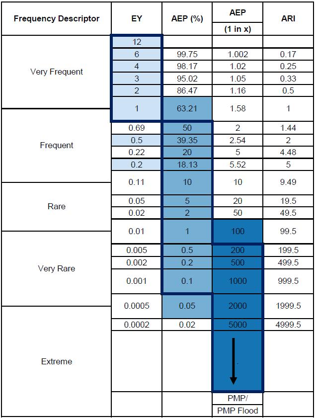
The ARR 2019 method provides patterns for 12 climatic regions across Australia, with Bulahdelah catchment falling within the Southern Semi-arid region. ARR 2019 provides patterns for each duration which are sub-divided into temporal pattern bins based on the frequency of the events. Figure 6 6 shows the categories of bins (very frequent, frequent, rare, very rare and extreme) and corresponding AEP groups. At the time of the model update, the “very rare” bin had been unavailable and was not used in this flood study; instead, temporal patterns from the “rare” bin were applied for the 1 in 200 and 1 in 500 AEP events. There are ten temporal patterns for each AEP/duration in ARR 2019 that have been utilised in this study for the 20% event to 1 in 500 AEP events.

Temporal patterns for this study were obtained from the ARR 2019 Data Hub (http://data.arrsoftware.org/). A summary of the data hub information at the catchment centroid is presented in Appendix D . The method employed to estimate the PMP utilises a single temporal pattern (Bureau of Meteorology, 2003), as is consistent with ARR 2019.

6.2.6 ARR 2019 areal temporal patterns

ARR 2019 recommends that Areal Temporal Patterns (ATP) should be considered in catchments larger than 75 km2 to account for the spatial smoothing of rainfall that occurs over larger catchments. Bulahdelah catchment covers an area of over 430 km2 which is above the threshold of considering ATPs. ATPs are applicable for storm durations including and greater than 12 hours. Hence, ATPs were applied when assessing longer durations above or equal to this threshold in the hydrologic model.

6.2.7 Areal reduction factors

ARFs are defined as an estimate of how the intensity of a design rainfall event varies over a catchment The main assumption in this estimate is that large catchments will not have a uniform depth of rainfall over the entire catchment.The ARFs were derived from the ARR 2019

Data Hub and applied in the WBNM models for all of the investigated design storm events. The ARF varies with AEP and duration and the resulting set of ARFs for the design storms are provided in Appendix D The ARF for the PMF has been set as 1 as per ARR 2019 recommendations.

6.3 Comparison with “At Site” and ARR 1987 data

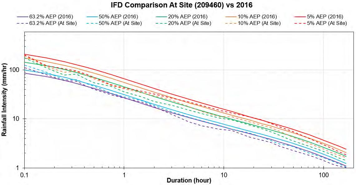
The 2016 IFD curves from the Bureau of Meteorology were compared to the IFD created using the “At Site” rainfall gauges available in the vicinity of the study and the results are presented on Figure 6.7. The Bulahdelah Station (Station ID: 209460) had the highest sampling frequency and was used to determine the “At Site” IFD for events up to the 5% AEP. The relatively short period of record did not allow estimates of rarer events. It is noted that the 2016 and the “At Site” IFDs are typically consistent with the largest difference observed for durations of less than 1 hour.

The 2016 IFD were also compared to the 1987 IFD and the results are presented on Figure 6.8. It is observed that the 2016 IFD rainfall intensities are consistent with the 1987 IFD for frequent events and for long durations. The 2016 IFD rainfall intensities are higher than the 1987 IFD intensities for 10% AEP and rarer events particularly for shorter durations.

The 2016 IFD were adopted for this study as per ARR 2019 requirements.

6.4 Design events

The design events modelled in this study include:

• Frequent events – 20% AEP

• Rare events – 5% AEP and 1% AEP

• Very rare events – 1 in 200 AEP and 1 in 500 AEP

• Extreme event – Probable Maximum Flood (PMF)

The terminology of these events is defined as per the ARR 2019 guidelines presented in Figure 6.6. All events (except the PMF) use spatial and temporal patterns provided by the ARR 2019 Data Hub. The PMF uses a combination of other temporal and areal patterns as described in the following section.

6.5 Probable Maximum Flood event

The Probable Maximum Flood (PMF) is the largest flood event resulting from the Probable Maximum Precipitation (PMP). The PMP rainfall depth has been estimated using the ARR 2019 guidelines. According to the PMP method zones diagram (Bureau of Meteorology, 2003) Bulahdelah catchment fall within the GSAM-GTSMR Coastal Transition Zone. Therefore, durations of up to 6-hours have been considered for the PMP in accordance with the Generalised Short Duration Method (GSDM) derived by the Bureau of Meteorology (BoM) (Bureau of Meteorology, 2003) and durations of 24 hours or longer have been estimated using both the Generalised Southeast Australia Method (GSAM) (Bureau of Meteorology, 2006) and the Generalised Tropical Storm Method (GTSMR) (Bureau of Meteorology, 2005) Intermediary durations (i.e. 9 hr, 12 hr and 18 hr) have been estimated using all three methods and the maximum has been used for the PMF. A summary of the GSDM, GSAM and GTSMR results were provided in Table 6.2, Table 6.3 and Table 6.4, respectively