Engineering Design Problems

3.

Desired oscillations a. With R = 1 kΩ and C = 1µF, sketch the pole locations as the gain K varies from 0 to ∞, showing the scale for the real and imaginary axes. Find the K for which the system is barely stable and label your sketch with that information. What is the system’s oscillation period for this K? or reach us at - www.matlabassignmentexperts.com b. How do your results change if R is increased to 10 kΩ?

The following feedback circuit was the basis of Hewlett and Packard’s founding patent.

You can control the steering-wheel angle w(t), which causes the angle θ(t) of the car to change according to where d is a constant with dimensions of length. As the car moves, the transverse position p(t) of the car changes according to

Consider three control schemes: a. w(t) = Ke(t) b. w(t) = Kve˙(t) c. w(t) = Ke(t) + Kve˙(t) where e(t) represents the difference between the desired transverse position x(t) = 0 and the current transverse position p(t). Describe the behaviors that result for each control scheme when the car starts with a non-zero angle (θ(0) = θ0 and p(0) = 0). Determine the most acceptable value(s) of K and/or Kv for each control scheme or explain why none are acceptable.

Part a. This system can be represented by the following block diagram:

We are given a set of initial conditions — p(0) = 0 and θ(0) = θ0 — and we are asked to characterize the response p(t). Initial conditions are easy to take into account when a system is described by differential equations. However, feedback is easiest to analyze for systems expressed as operators or (equivalently) Laplace transforms. Therefore we first calculate the closed-loop system function, which has two poles: ±jω0 where ω0 = V We can convert the system function to a differential equation: and then find the solution when x(t) = 0, so that p(t) = C sin ω0t since p(0) = 0.

From p(t) we can calculate θ(t) = ˙p(t)/V = C/V ω0 cos ω0t. From the initial condition θ(0) = θ0, it follows that C = V θ0/ω0 and for t > 0.

If K is small, then the oscillations are slow, but they have a large amplitude. If K is large, then the oscillations are fast (and therefore uncomfortable for passengers), but the amplitude is small. While none of these behaviors are desireable, it would probably be best to increase K so that the amplitude of the oscillation is small enough so that the car stays in its lane.

Part b. The system can be represented by the following block diagram:

The closed-loop system function is

We would like to make Kv large because large Kv leads to fast convergence. Large values of Kv also lead to smaller steady-state errors in p(t).

There are no oscillations in p(t) with the velocity sensor, which is an advantage over results with the position sensor in part a. However, there is now a steady-state error in p(t), which is worse. Fortunately the steady-state error can be made small with large Kv.Part c. The system can be represented by the following block diagram:

The closed-loop system function is

=

There is an enormous variety of acceptable solutions to this problem, since there are many values of K and Kv that can work. Here, we focus on one line of reasoning based on our normalization of second-order system in terms of Q and ω0.

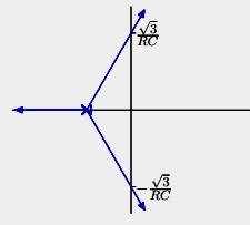
To avoid excessive oscillations, we would like Q to be small. Try Q = 1. Then

Then p(t) has the form

As before, we can use the intial condition of θ(0) = θ0 to determine C. In general, θ(t) = ˙p(t)/V so p˙(0) = θ0V = C √ 3ω0/2. Therefore