Yagi Antenna theory, free of mathematics

YAGI ANTENNA THEORY, MATH FREE

Author: Eng. Martin Lema

Revision date: July 2022

Scope

On the Internet and in antenna books there are lots of graphics, plans and tables concerning the design of Yagi antennas. They mostly contain valid data as they are generally based on real experiments or measurements of antennas that exist and work. But there is few information about the principle of operation of these antennas. In classic books of antennas (for university students) the theory is well developed, but it happens that either they are not available to the amateur experimenter or contain mathematical expressions too complex for them. Understanding the operation (even without analytical expressions) allows the experimenter to "know what happens if modifies something ". If you do not know the operation principles, you have no degrees of freedom to act if you find a plane on which you want to experiment and don´t get pipes of the exact size, or want to change the working frequencies, etc. For the telecommunications students, this article will help them to "understand the antenna" before starting a deep theoretical study. It is quite common for a student to be required to explain the theory of something he never saw, and does not know what it is for, or how it works. With these goals in mind, this article presents a conceptual explanation of how a Yagi antenna works. As I anticipated a few paragraphs before, making a thorough analysis requires quite complicated mathematics and concepts of matrix calculus of mutual impedances, electromagnetism, and other knowledge necessary for a deep and professional study, which will not be addressed here. The objective is that the reader understands the operation and can make a basic sizing of a Yagi antenna.

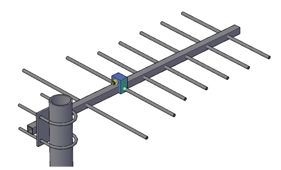
Yagi antenna overview

It consists of an antenna formed by a driven element and several parasitic passive elements. The typical configuration consists of three types of elements, one driven, one slightly longer than the driven called the reflector, and several, barely shorter than the driven called the directors. It is a simple antenna to machine, very cheap from the point of view of materials and labor, with a single connection so it has practically no possible points of failure (except the connection). This type of antenna is characterized by moderate gain (no more than 12 dBd) and operates in a limited bandwidth. If you are looking for more gain or directivity you already must think about antennas with reflector as parabolic (clearly in the microwave range, a parabolic reflector in HF is not practicable) and if you are looking for more bandwidth, you must think of an antenna of the logperiodic type. Typically, they have one reflector and N directors, usually up to 12 and no more than 20 because as the number of directors increases, they have less and less impact on the directivity of the set.

This antenna was developed in Japan in the mid-20s by Hidetsugu Yagi and Shintaro Uda. Different historians do not agree if Yagi is the inventor and Uda the co-inventor or vice versa.

For starting, a little of antenna theory

An antenna of only one element will always have an omnidirectional pattern, this element can be for example a dipole. No matter how much we experience variants of a dipole, make it shorter or longer, or have a different conductor section, we will get its radiation pattern to be different and its characteristic impedance to be different, but it will always be omnidirectional.

If we want an antenna to be directional, we have only two possible options:

 Put some type of reflective surface near it (such as on a satellite dish, panel, or dihedral antenna)

 Assemble an array or formation with at least 2 elements (as in a Yagi, logperiodic or other arrays)

As this article is focused on Yagi antennas, we will analyze the option of making an antenna directional if it is composed of 2 or more elements (typically much more than two).

All antennas are scalable. If we multiply by a constant K all the dimensions of an antenna that was designed for a certain frequency F, we will have an antenna with exactly the same performance at the frequency F/K. This is an invaluable tool for the experimenter and little spread in the amateur world. This principle applies to all antennas of the standing wave type (Dipoles, monopoles, Yagi, logperiodic, collinear, etc.). These are all the "standard" antennas.

For example, if we find a Yagi antenna that works with a certain directivity and radiation pattern at 335 MHz and we want one that works exactly in the same way, but at 430 MHz we simply multiply all the dimensions of the original by 335/430 = 0.779 and it results in an antenna at 430 MHz with the same gain, radiation pattern, impedance etc.

Beware that when I say all dimensions, means that are all, i.e. up to the diameters of conductors, separations etc.

Antenna arrays

We already know that, if we have an antenna made of only one element without reflectors or ground plane or anything around it, its radiation pattern will always be omnidirectional. But if we have two or more antenna elements connected to the same equipment we can achieve different radiation patterns, which are even directional (with some configurations, not all). This is what we know as "antenna arrays” or antenna formations. So, for creating an antenna array it is needed at least two antennas, and they must be connected in some way to the equipment. This article does not explore into interconnection techniques, the topic of arrays is mentioned only to have some theoretical support when we finally reach the Yagi antennas.

Broadside formation (one above the other as in an FM station)

End fire formation (one in front of the other)

The shape of the radiation pattern of an array of N elements has a mathematical expression that I will not bring to this article (I promised not to use complicated mathematics) but, from this expression we can determine that:

 The maximum gain obtainable from the formation will be N times the gain of each element of the formation (in gain times, not in dB). Note: I said the maximum obtainable, not that it always has N times the gain of each element.

 The shape of the radiation pattern depends on the phase with which each element is fed, the distance between elements and their relative position.

 Broadside dipole arrays are always omnidirectional.

 End fire dipole arrays can be directional to one side, or the other depending on the separation and phase with which each dipole is fed. They can also be omnidirectional under certain circumstances.

How is phase rotation achieved? Every time the RF signal travels a wavelength (λ) within a cable, it rotates 360°, if it travels half a wavelength, it rotates 180° and so on. If it travels 1.5 wavelengths it is the same as having traveled 0.5 wavelengths, since when it traveled one, it rotated 360 ° (that is, it has the same phase as at the beginning) and in the remaining half wavelength, it rotates 180 °.

The propagation speed within a cable (coaxial or whatever) is always lower than that of propagation in the air, this must be considered to calculate the wavelength inside the cable, but this is not necessary for the purpose of this article.

A simple example of end fire array

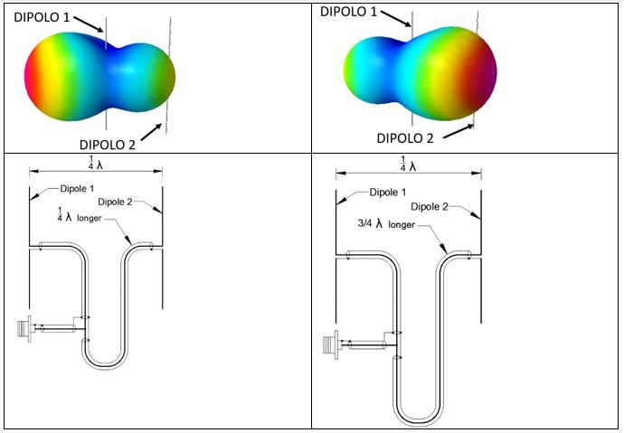
Next, I will show an example of an array of two dipoles in end fire configuration (one in front of the other), this configuration is not practical to be built, but provides the necessary foundations to understand the operation of a Yagi type antenna. "Not practical" means that it requires cables, connectors, splices, a lot of work on impedance matching, etc. As we will see later it can be solved with a Yagi type configuration that is infinitely simpler. But this development will provide the reader with the necessary elements to understand a Yagi without using advanced mathematical expressions.

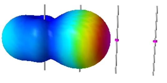
In this first example we will analyze two situations. In both cases both dipoles are fed from the same point, but with wires of different lengths, in one case one of the wires is 1/4 wavelength longer than the other, and in the other case it is 3/4 wavelength longer. I arbitrarily chose a separation between dipoles of 1/4 wavelength. It should be clarified that this example did not consider impedance adaptation, it is not necessary to analyze directivity. In the case of 1/4 λ the phase with which the second dipole is fed rotates 90° while in the case of 3/4 λ it rotates 270°. Then I performed the simulation to see what radiation pattern results in each case. For the graphics in this article, I used the electromagnetic simulation software 4NEC2. Such software is available for free on the Internet, is very friendly and can be used freely for experimental or didactic purposes (as in this article). It is very accurate and the results it shows are very consistent with reality. In fact, it is used to "experiment" with antennas, then build them, and the performance is very close as simulated. From observing the results, we can see that even with the same physical configuration, with the same separation between the dipoles, just by modifying the phase we achieve that the radiation pattern is quite directional to one side or the other. In the graph obtained with the 4NEC2 the colors magenta and red represent higher power density while light blue and blue represent lower radiated power density in that sense.

With this example we can visualize that, given a structure with at least two elements, even without changing its physical configuration at all, different radiation patterns can be achieved by simply modifying the phase with which each of these elements is fed.

Now one step more, let's do this with four elements

At least intuitively we can deduce that:

 With more than two elements (3, 4 or whatever) this effect of increasing directivity should be more noticeable.

 If we want the solution to be directional, taking one as a reference, all those who are on one side (where you want to direct the energy) must have some phase rotation with respect to the previous one.

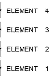
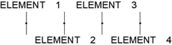
Following the same criteria as the previous example with just two elements, we will do this with four elements, also separated 1/4 λ and with phase rotation of -90° between elements (that is, if the first is assigned 0° (reference), the second will rotate -90°, the third -180° and the fourth -270°.

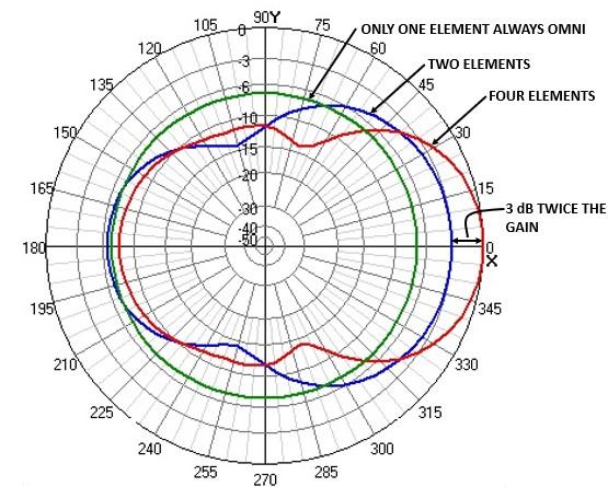
Comparing the three radiation patterns we can affirm that:

 Just one element is always omnidirectional.

 Two elements already make it slightly directional.

 Four elements make it more directional, and the gain increases 3 dB that is, it is double what it had with 2 elements (it coincides with the theory, obviously)

Note: due to the way the 4NEC2 graphs are shown, when comparing radiation patterns, the one with the higer gain has assigned the value 0, so the two elements have a maximum of -3 dB, which means that it has 3 dB less gain than the one it takes as a maximum.

How did we arrive at the Yagi from this?

Recapitulating what we saw so far, we can say that:

 If we have a single dipole without reflectors (in free space), the radiation pattern will always be omnidirectional.

 If we have two or more dipoles facing each other (end fire configuration) the resulting radiation pattern may be directional to one side or the other depending on the formation (depends on the relative phase with which the dipoles are fed)

 This configuration seen, it is possible to assemble, and it works, but it is very complicated, it is full of cables, connectors, splices.

Although the subject was superficially named, all interconnections between elements require impedance adaptation that, although possible, is a stumbling block if you try to put together this configuration in practice.

What did Mr. Yagi, to implement this configuration without using cables or connectors or anything?

Very simple, instead of interconnecting the elements with cables, he left only one connected to the equipment and the rest are coupled in electromagnetic form. That is, the current flowing through the driven element induces current in its neighbors. It is intuitive to think that the closer an element is to its neighbor, the stronger the coupling. For that reason, the separation between elements of any Yagi antenna is of the order of 0.1λ to 0.2λ (and in HF Yagis even less for a matter of size) So far it seems simple, but how do we make the phase appropriate so that the antenna is directional for the side we want it to be?

To understand this, we must go a little deeper into antenna theory (as promised, without mathematics)

We know that a dipole resonates at a certain frequency. What does it mean that it resonates? Well, resonance occurs when the impedance it presents is purely resistive, this means that if we apply a signal to a perfect dipole in free space whose frequency is just the resonance, the voltage and current will be in phase (it behaves as if it were a resistor, clearly it is not, because it is an antenna), But voltage and current are in phase. In electricity that is known as pure active power and there is no reactive power. If the value of the impedance of the dipole (which in the resonant frequency is pure resistive), coincides with the impedance of the cable, there will be nothing reflected (VSWR = 1: 1). But if the frequency with which I feed that dipole is different from that of resonance, the impedance is never pure resistive, then the current circulating will not be in phase with the applied voltage. This in electricity is called apparent power (it is formed by active power and reactive power), the active is radiated and the reactive returns to the transmitter. That is, the SWR is no longer 1:1 although the resistive part of the impedance of the cable and the antenna coincide. In other words, if we feed a dipole with a frequency outside the resonance, it will always present VSWR.

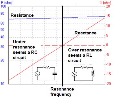
Now, making use of the same simulator that we use to analyze the shape of the radiation pattern, we will see how is the impedance that a dipole presents in its resonance frequency and slightly above and below this frequency, if we use it above the resonant frequency it behaves like an inductive circuit, That is, the reactive power it presents is of the inductive type, while if we use it below the resonance frequency, it behaves as capacitive.

Herein lies the genius of Mr Yagi's invention.

If we feed a dipole with a signal of its resonance frequency, clearly the electromagnetic fields around it will be of that same frequency and as it is in resonance the current that circulates will be in phase with the voltage.

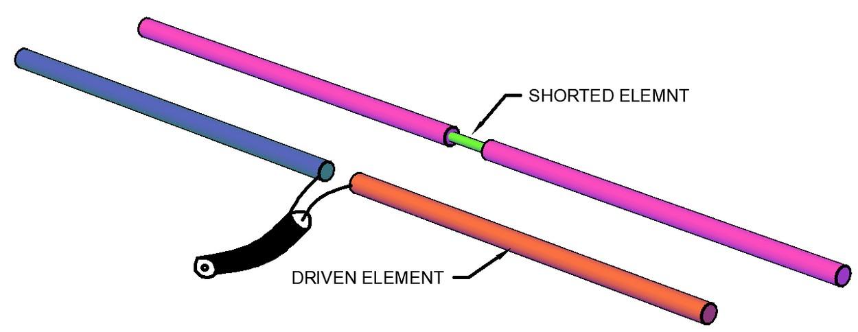
If we approach a dipole that is slightly shorter than the driven dipole, this second dipole will have a higher resonant frequency than the signal in its environment. (If the dipole is shorter the resonance frequency will be higher). Then it is being used below its resonance frequency. In this case it behaves as capacitive and in any capacitive circuit the current advances the voltage. For current to circulate this dipole must be shortcircuited, that is, the two halves of the dipole are joined.

And, if we approach a dipole that is slightly longer than the driven dipole, this second dipole will have a lower resonant frequency than the signal in its environment. (If the dipole is longer the resonance frequency will be lower). So, it's being used above its resonant frequency. In this case it behaves as inductive and in any inductive circuit the current delays the voltage. It must also be short-circuited.

Only for didactic purposes the element is shown in short circuit as if it were formed by two pieces, in practice it is a single whole pipe

In this way, just by putting the elements on one side and the other of the driven element, one longer and the other shorter, we have the whole problem solved. we have a formation of antennas, with elements whose phase on one side delays and on the other side advances. It only remains to determine which side is which side (that is, how I determine for which side the antenna focuses the power). Again, here I will use

simulation, as analytical development is too complex and makes no sense for the purposes of this article.

The importance of the reflector

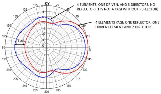
The reflector element (the longest) has a very important function in the Yagi since it is responsible for improving the front-back relationship, that is, it greatly reduces the energy that the antenna radiates "backwards". Although without analytical developments and only intuitively we now know that the "director" elements, being a little shorter than necessary for resonance, behave as capacitive and the current that circulates through them has such a phase that it causes the energy that advances from the driven element to be added in phase as it passes through the directors. This let us to think that, if we put a longer element, in which we already know that the phase rotation is the opposite of that of the directors, the behavior will be the opposite, that is, it will prevent the energy emitted by the driven element from advancing in the direction of the reflector (and that is why it is called reflector). There is a principle of physics that is strictly fulfilled and is that energy cannot be created and cannot disappear, so what does not radiate backwards (because the reflector prevents it), where does it go?, the answer is predictable: to another side that is not behind, that is, to the side of the main lobe (although it also creates secondary lobes).

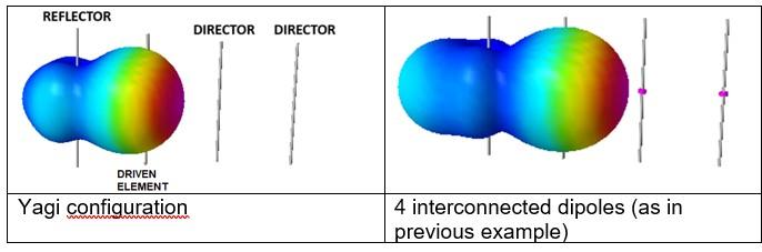
For example, given a 4-element antenna, a 2-director-and-reflector Yagi has a much better front-to-back ratio and is more directive than a 3-director without a reflector (it wouldn't be Yagi). In fact, no Yagi antenna implementation omits the reflector.

The quantity and separation between elements

Using only common sense we can obtain the following conclusions.

1. As the coupling between elements is based on the proximity of the elements, if they are very far apart, they do not interact (or do very little) and stop working properly.

2. On the contrary, if they are very close to each other, there is not enough phase rotation for the phenomena described above to occur (in addition all the elements would be screened from each other)

3. So, the optimal point will be given with a separation that is in some intermediate value between elements very close to each other and very far from each other.

4. Within the possible range (i.e. neither glued nor too far away) it is obvious that if they are further away the antenna will be longer.

The study of the relationship between separation and characteristics of the Yagi antenna as an assembly is very complex and far exceeds the scope of this article. In fact, it is not even possible to do analytically, there are tables and graphs based on measurements on real antennas and also based on simulations.

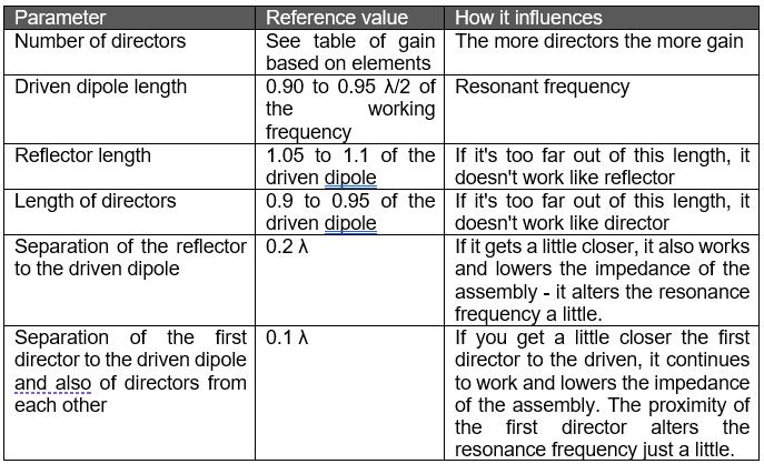
But we can say that based on experience, a reasonable separation between reflector and driven element (and widely used in practice with real antennas) is of the order of 0.2 λ.

Regarding the separation between directors and between the first director and the driven element is usually between 0.1λ and 0.3λ. It is obvious that 0.1λ makes the set shorter, but it is difficult to obtain a gain greater than 8 or 9 dBd.

Regarding the quantity, it is obvious that the greater the quantity, the greater the gain. But there are practical limits. As the number of directors increases, the contribution of each one becomes smaller until there comes a time when they no longer contribute. Under this reasoning, the first director is the one that contributes the most to improve the gain since it is the closest to the driven element and therefore the one that captures the most energy from the driven and "retransmits" it with the appropriate phase, the second already receives less, the third less and so on until the last. The following table, shows the gain obtainable with different number of elements and separations between directors between 0.1 λ and 0.2λ. This is an indicative table and different designers will get different gains with the same number of elements.

But it will always be maintained at least the order of magnitude indicated here. The number of elements in this table includes the reflector and the driven element. For example, the 5-element Yagi with 11 dBi gain has 3 directors, one reflector and the driven element.

The impedance and separation between the driven element and its two neighbors

So far, we talk about the separation between elements only from the point of view of phase rotation, but there is an aspect that is critical, and it occurs when we approach

the first director and the reflector to the driven element, there the impedance presented by the connection point of the set is strongly altered. The impedance of a dipole if it were alone (with nothing around, no ground plane or anything) is 73 Ω when used at its resonant frequency. The presence of the two neighboring elements (the reflector and the first director) causes the impedance to be significantly altered and can easily reach 15 or 20 Ω. A common solution is that the driven element is made with a folded dipole, this configuration allows to raise the impedance 4 times. So, if we bring the parasitic elements close enough so that the impedance of the dipole is close to 12.5 Ω, when raised 4 times it reaches the desired 50 Ω in any telecommunications antenna (or 75 Ω in TV antennas). Another possible solution, also very common is a "Gamma Match" that consists of a section parallel to the main element with capacitive coupling. This adapter allows to adapt impedances over a very large range with separate settings for the resistive (moving part) and reactive (coupling capacitor) part.

The design of the driven-reflector-first director element assembly is too complex to summarize in an article like this. In general, the solution is found by simulation. This set of director and reflector, determines the impedance and working frequency of the antenna, the addition of directors has a lot of weight in the gain, but practically does not alter other parameters of the antenna as a set. The interaction of the three elements also influences the resonant frequency of the whole.

Reference values or starting points for a design.

The following reference values are used to aim a Yagi antenna project, as initial values for a simulation or even direct experimentation. The support boom is not part of the antenna, so it has no effect at the RF level and can be of any material, shape, and section. Its only function is to give mechanical rigidity to the whole. Regarding the diameter of the elements, they have some effect on the resonance frequency and the bandwidth of the set (little, but it influences). Larger diameters cause the dipole to resonate at lower frequencies. Considering this effect, it is that the main dipole is not half-wave but 0.90 to 0.95 λ/2. This range of values applies in diameters of elements that are used in practice (between 3mm and 10mm)

For experimenters, a good starting point is to use the data in the table above to start the simulation in 4NEC2, MMANA-GAL or other electromagnetic simulation tools and "play" with the different measurements until the desired performance is achieved. The great advantage we have today with these simulators (and those, like me, who experimented with antennas, 40 years ago we didn´t have it) is that there is no need for physical tools, nor is material wasted during experimentation. Another of the great advantages of simulation is that exotic shapes can be experienced, which is virtually impossible with analytical developments still very advanced, which were limited to forms with simple mathematical expressions (segments, circles, ellipses, spirals, etc.). Experimenters should always remember that the antennas are all scalable, that is, if in the simulation it works fine or we have a plane of an antenna that works well, but at another frequency it is simple to take it to the frequency we want it to work, we just have to scale the dimensions.

Final considerations

Using the criteria descripted in this article can help the experimenter or the student to decide with technical reason, when to go a little far from a calculated dimension or length or position of an element. For example, after reading this it is clear that the reflector must be longer than the driven and the director shorter, if it is not thus: DOESN´T WORK THE YAGI. But it is not very important if it is 5% or 10%, this do not modify its function.

Another example is the diameter of the elements, if it differs a little from calculated, nothing important happens. For example, if you scale an antenna whose original design uses elements with a diameter of 6 mm, and after scaling them results in a pipe of 4.78 mm. Where do you get a 4.78 mm pipe? Now you know that in this case is the same 6 or 5 mm or the pipe you can find. The same with separations, between reflector-driven-first director impacts strong in impedance and a little in resonance frequency but has a minimal importance in the radiation pattern.

Summarizing: Knowing deeply how it works, what dimension or size influence in what parameter, and using electromagnetic simulators, any antenna should be designed and will work fine when finally, will be built.