Issuu

EssentialGuide toFeature Engineering

Turnrawdataintosignal:encode,scale, transform,andpipelinewithpandasand scikit-learn.

Apracticalguidetoencoding,scaling,transforming,andpipingdata intomodel-readyfeatureswithpandasandscikit-learn.

EssentialGuideto FeatureEngineering

IbonMartínez-Arranz

IterativeImputer(multivariate,model-based)...............119

Visualcheck:distributionbefore/a erimputation(addsvalue).....121

Leakage-safeevaluation:quickcomparison...............122

Summary..................................124

IntroductionandSetup

WhatisFeatureEngineering?

Featureengineeringistheartandscienceoftransformingrawdataintomeaningful variables(features)thatamachinelearningmodelcane ectivelyuse.

Atypicaldatasetisrarelyreadytobefeddirectlyintoanalgorithm. Categoricalvariables,missingvalues,di erentscales,orskeweddistributionscan allreducemodelperformanceorevencausefailures.

Featureengineeringinvolvestaskssuchas:-Convertingcategoriesintonumbers (encoding).-Scalingandnormalizingnumericalvariables.-Applyingtransformationstoimprovedistributions.-Creatingnewfeaturesfromexistingones.Handlingmissingvaluesconsistently.

Inthisbook,wewillgothroughthesestepsusingpracticalexamplesin Python, mainlywith pandas and scikit-learn.

WhyisFeatureEngineeringImportant?

Machinelearningalgorithms,nomatterhowsophisticated,cannotfullycompensateforpoorlyprepareddata.

• Astrongmodelwithbadfeatures → poorresults.

• Asimplemodelwithwell-cra edfeatures → surprisinglygoodresults.

Inpractice,mostmachinelearningprojectsspendmorethan 70%ofthetimeon preprocessingandfeatureengineering,notonmodeltuning.

Thisdocumentwillcover:-Encodingofcategoricalvariables.-Scalingandnormalizationofnumericalvariables.-Variabletransformations(log,Box-Cox,YeoJohnson).-Featurecreation.-Missingvalueimputation.-Pipelinesforreproducibility.

LibrariesUsedinThisBook

Wewillrelyonthefollowinglibraries:

• pandas → handlingtabulardata(load,clean,transform).

• numpy → e icientnumericaloperations.

• scikit-learn → preprocessingtools(OneHotEncoder, StandardScaler , PowerTransformer, Pipeline,etc.).

• matplotlib and seaborn → visualizationofdistributionsandresults.

Let’simportthemandcheckthateverythingisworking.

1 import numpyasnp 2 import pandasaspd 3 import matplotlib.pyplotasplt 4 import seabornassns

5 6 from sklearn import datasets 1 import numpyasnpy 2 import pandasaspd 3 import matplotlib.pyplotasplt 4 import seabornassns

5 6 from sklearn import datasets

ExampleDatasets

Wewillusesomeclassicalmachinelearningdatasets,easilyavailablefrom scikit -learn or seaborn:

• Titanicdataset (survivalofpassengers). Usefultoworkwithcategoricalvariables,missingvalues,andencoding.

• Irisdataset (classiﬁcationofﬂowersbasedonmeasurements). Perfectforscaling,transformations,andsimplepipelines.

• CaliforniaHousingdataset (predictionofhouseprices). Goodfornumericfeatures,scaling,andfeaturegeneration.

Let’sloadthem.

1 #Irisdataset

2 iris = datasets.load_iris(as_frame=True) 3 iris_df = iris.frame

5 #Californiahousingdataset

6 housing = datasets.fetch_california_housing(as_frame=True )

7 housing_df = housing.frame

9 #Titanicdataset(fromseaborn)

titanic_df = sns.load_dataset("titanic")

12 print("Irisshape:", iris_df.shape) 13 print("Housingshape:", housing_df.shape) 14 print("Titanicshape:", titanic_df.shape)

1 #Irisdataset

2 iris = datasets.load_iris(as_frame=True) 3 iris_df = iris.frame

5 #Californiahousingdataset

6 housing = datasets.fetch_california_housing(as_frame=True )

QuickOverviewoftheDatasets

IrisDataset

• 150samples,4numericalfeatures(sepallength/width,petallength/width).

• Target:speciesofirisﬂower(Setosa,Versicolor,Virginica).

• Goodforclassiﬁcationtasks.

1 #Quickpeekateachdataset

2 display(iris_df.head())

1 #Quickpeekateachdataset

2 display(iris_df.head())

sepallength(cm)

sepalwidth(cm)

petallength(cm)

petalwidth(cm)

target

CaliforniaHousingDataset

• 20,640samples,8numericalfeatures(medianincome,averagerooms,latitude,longitude...).

• Target:medianhousevalue.

• Goodforregressiontasks.

• 891passengers,mixofcategoricalandnumericalfeatures(sex,age,class, embarked...).

• Target:survival(0=died,1=survived).

• Goodforpreprocessingdemonstrations(encoding,imputation).

1 #Quickpeekateachdataset 2 display(titanic_df.head())

Thishelpsussee:-Whichvariablesarenumericvscategorical.-Ifvariableshave di erentscales.-Ifdistributionsareskewed.-Howdatasetsdi erincomplexity.

Let’splotsomehistogramsforeachdataset.

1 #HistogramsforIrisdataset

2 iris_df.hist(figsize=(3*3,2.5*2), bins =15, layout = (2,3), color = "#FECB00", edgecolor = '0.3',)

3 plt.suptitle("IrisDataset-FeatureDistributions", fontsize=14)

4 plt.show()

1 #HistogramsforIrisdataset

2 iris_df.hist(figsize=(3*3,2.5*2), bins =15, layout = (2,3), color = "#FECB00", edgecolor = '0.3',)

3 plt.suptitle("IrisDataset-FeatureDistributions", fontsize=14)

4 plt.show()

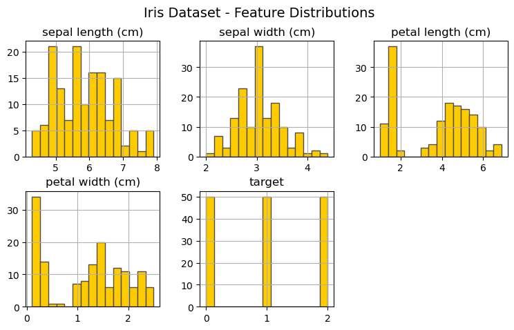
Figure1: Imagegeneratedbytheprovidedcode.

1 #HistogramsforCaliforniaHousingdataset

2 housing_df.hist(figsize=(3*3,2.5*3), bins =15, layout = (3,3), color = "#FECB00", edgecolor = '0.3',)

3 plt.suptitle("CaliforniaHousingDataset-Feature Distributions", fontsize=14)

4 plt.show()

1 #HistogramsforCaliforniaHousingdataset

2 housing_df.hist(figsize=(3*3,2.5*3), bins =15, layout = (3,3), color = "#FECB00", edgecolor = '0.3',)

3 plt.suptitle("CaliforniaHousingDataset-Feature Distributions", fontsize=14)

4 plt.show()

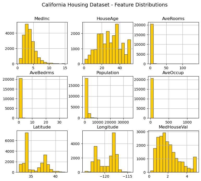
Figure2: Imagegeneratedbytheprovidedcode.

1 #HistogramsforTitanicdataset(numericfeaturesonly)

2 titanic_df.select_dtypes(include=["float64", "int64"]). hist(figsize=(3*3,2.5*2), bins =15, layout =(2,3), color = "#FECB00", edgecolor = '0.3',)

3 plt.suptitle("TitanicDataset-NumericFeature Distributions", fontsize=14)

4 plt.show()

1 #HistogramsforTitanicdataset(numericfeaturesonly)

2 titanic_df.select_dtypes(include=["float64", "int64"]). hist(figsize=(3*3,2.5*2), bins =15, layout =(2,3), color = "#FECB00", edgecolor = '0.3',)

3 plt.suptitle("TitanicDataset-NumericFeature Distributions", fontsize=14)

4 plt.show()

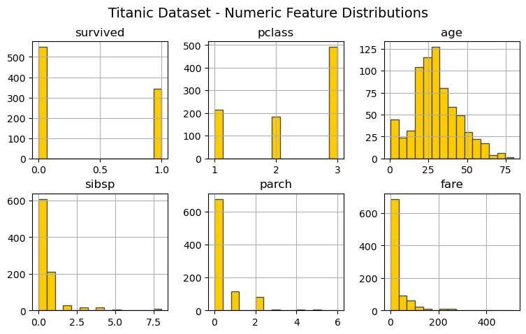
Figure3: Imagegeneratedbytheprovidedcode.

Nowthattheenvironmentissetupandwehaveaﬁrstlookatthedatasets, inthenextchapterswewilllearnto:

1.Encodecategoricalvariables(labelencoding,one-hot,ordinal).

2.Scaleandnormalizenumericalvariables. IbonMartínez-ArranzPage17

3.Transformdistributionswithlog,Box-Cox,andYeo-Johnson.

4.Createnewfeaturesandhandlemissingvalues.

5.Buildcompletepreprocessingpipelinesforreproducibilityandproduction.

Withthis,wearereadytomoveto Chapter2:EncodingCategoricalVariables.

EncodingCategoricalVariables

CategoricalvsNumericalFeatures

Numericalfeatures aremeasuredonanumericscale(e.g., age, fare, sepal_length).

Categoricalfeatures representdiscretegroupsorlabels(e.g., sex, class, embarked).

Somecategoricalfeaturesare ordinal (theyhaveaninherentorder,e.g., low < medium < high),whileothersare nominal (noorder,e.g., red, green, blue).

Whythismatters:

• ManyMachineLearningalgorithmsrequirenumericinput.Categoricalvariablesmustbeencoded.

• Thechoiceofencodingdependsonwhetherthecategoryis ordinal or nominal.

• Forhigh-cardinalitycategories(hundreds/thousandsofuniquevalues),naive one-hotencodingcanexplodedimensionality.

Belowwe’llinspecttheTitanicdatasettoidentifycategoricalvsnumericalcolumns andlookattheirdistributions.

dtype survived int64 pclass int64 sex object age

ﬂoat64 sibsp int64 parch int64 fare ﬂoat64 embarked object class category who object adult_male

1 Categoricalcolumns:['sex' , 'embarked' , 'class' , 'who' , 'adult_male' , 'deck' , 'embark_town' , 'alive' , 'alone' ]

2 Numericalcolumns:['survived' , 'pclass' , 'age' , 'sibsp' , 'parch' , 'fare']

1 #Plotdistributionsforsomecommoncategorical variables

2 fig, axes = plt.subplots(1,3, figsize=(12,4))

sns.countplot(data=titanic_df, x="sex", ax=axes[0], palette =['#fecb00ff' , '#6b99a6ff'])

4 axes[0].set_title("sex")

sns.countplot(data=titanic_df, x="class", ax=axes[1], palette =['#b7d3dbff' , '#6b99a6ff' , '#3a6674ff'])

7 axes[1].set_title("class")

9 sns.countplot(data=titanic_df, x="embarked", ax=axes[2], palette =['#ffef80ff' , '#fecb00ff' , '#cc9b00ff'])

10 axes[2].set_title("embarked")

11 plt.tight_layout()

12 plt.show()

1 #Plotdistributionsforsomecommoncategorical variables

2 fig, axes = plt.subplots(1,3, figsize=(12,4))

3 sns.countplot(data=titanic_df, x="sex", ax=axes[0], palette =['#fecb00ff' , '#6b99a6ff'])

4 axes[0].set_title("sex")

sns.countplot(data=titanic_df, x="class", ax=axes[1], palette =['#b7d3dbff' , '#6b99a6ff' , '#3a6674ff'])

7 axes[1].set_title("class")

sns.countplot(data=titanic_df, x="embarked", ax=axes[2], palette =['#ffef80ff' , '#fecb00ff' , '#cc9b00ff'])

10 axes[2].set_title("embarked")

11 plt.tight_layout()

12 plt.show()

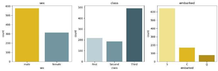
Figure1: Imagegeneratedbytheprovidedcode.

Takeaways

• sex, class,and embarked aretypical nominal/mixedcategoricalfeatures.

• class is ordinal onTitanic(Third < Second < First).

• High-cardinalitycolumnscancauseproblemsfornaiveone-hotencoding.

LabelEncoding(with sklearn.preprocessing.LabelEncoder)

LabelEncoding convertslabelstointegers {class_1:0, class_2:1, ...}.

Bestuse: encodingthe targetvariable(y) inclassiﬁcationproblems,ortruly ordinal featuresifyouunderstandtheimpliedordering.

Pitfall: UsingLabelEncoderon nominalfeaturecolumns injectsafakeorder(e.g., male=0, female=1),whichcanmisleadlinearanddistance-basedmodels. We’lldemonstrateitonthe Iris dataset’starget(speciesnames).

1 from sklearn.preprocessing import LabelEncoder 2 3 iris_df = sns.load_dataset("iris").copy() #speciesis stringlabels

4 y_str = iris_df["species"] 5 6 le = LabelEncoder()

7 y_encoded = le.fit_transform(y_str) 8

9 print("Classes:", list(le.classes_)) 10 print("Encodedsample:", y_str.head().tolist(), "->", y_encoded[:5].tolist())

1 from sklearn.preprocessing import LabelEncoder 2 3 iris_df = sns.load_dataset("iris").copy() #speciesis stringlabels

4 y_str = iris_df["species"] 5 6 le = LabelEncoder()

7 y_encoded = le.fit_transform(y_str) 8

9 print("Classes:", list(le.classes_)) 10 print("Encodedsample:", y_str.head().tolist(), "->", y_encoded[:5].tolist()) IbonMartínez-ArranzPage25

1 Classes:['setosa' , 'versicolor' , 'virginica']

2 Encodedsample:['setosa' , 'setosa' , 'setosa' , 'setosa' , 'setosa']->[0,0,0,0,0]

Whennottouseit: Do not use LabelEncoder fornominalfeatureslike sex or embarked unlessyouralgorithmistree-based(treesareinsensitivetomonotonic transformations).Forgeneralpipelines,prefer One-Hot or OrdinalEncoder (with explicitorder).

One-HotEncoding(pandas&scikit-learn)

One-HotEncoding(OHE) createsonebinarycolumnpercategory(e.g., sex_female, sex_male).

• Pros:safefornominaldata,widelyused.

• Cons:dimensionalityblow-upforhigh-cardinalityfeatures.

We’llshow:

1) pandas.get_dummies() —fastandconvenientforEDA/quickbaselines.

2) sklearn.preprocessing.OneHotEncoder —integrateswithpipelines/transformers(recommendedforproduction).

1 #One-Hotwithpandas.get_dummies()

2 titanic_small = titanic_df[["survived", "sex", "class", " embarked", "age", "fare"]].copy()

4 #drop_first=Truecanavoidthe"dummyvariabletrap"for linearmodelswithintercept

5 dummies_pd = pd.get_dummies(

6 titanic_small,

7 columns=["sex", "class", "embarked"],

8 drop_first=True #settoFalseifyouwantthefull setofdummies

9 ) 10 display(dummies_pd.head())

1 #One-Hotwithpandas.get_dummies()

2 titanic_small = titanic_df[["survived", "sex", "class", " embarked", "age", "fare"]].copy() 3

4 #drop_first=Truecanavoidthe"dummyvariabletrap"for linearmodelswithintercept

5 dummies_pd = pd.get_dummies(

6 titanic_small, 7 columns=["sex", "class", "embarked"],

8 drop_first=True #settoFalseifyouwantthefull setofdummies

9 ) 10 display(dummies_pd.head())

X = titanic_df.drop(columns=["survived"])

y = titanic_df["survived"]

categorical_features =["sex", "class", "embarked"]

numeric_features =["age", "fare"]

#Note:Forscikit-learn>=1.2usesparse_output=False; for<1.2usesparse=False

ohe = OneHotEncoder(handle_unknown="ignore", sparse_output=False, drop=None)

ct = ColumnTransformer(

transformers=[

("ohe", ohe, categorical_features),

("passthrough", "passthrough", numeric_features),

remainder="drop"

X_enc = ct.fit_transform(titanic_df) 23 feature_names = ct.get_feature_names_out() 24 print("Encodedshape:", X_enc.shape) 25 print("Samplefeaturenames:", feature_names[:10]) 1 #One-Hotwithscikit-learn'sOneHotEncoder+ ColumnTransformer

from sklearn.compose import ColumnTransformer

from sklearn.preprocessing import OneHotEncoder

X = titanic_df.drop(columns=["survived"])

y = titanic_df["survived"]

8 categorical_features =["sex", "class", "embarked"]

numeric_features =["age", "fare"]

#Note:Forscikit-learn>=1.2usesparse_output=False; for<1.2usesparse=False

ohe = OneHotEncoder(handle_unknown="ignore", sparse_output=False, drop=None)

ct = ColumnTransformer(

transformers=[

("ohe", ohe, categorical_features),

("passthrough", "passthrough", numeric_features),

], 19 remainder="drop"

)

22 X_enc = ct.fit_transform(titanic_df) 23 feature_names = ct.get_feature_names_out() 24 print("Encodedshape:", X_enc.shape) 25 print("Samplefeaturenames:", feature_names[:10])

1 Encodedshape:(891,11)

2 Samplefeaturenames:['ohe__sex_female''ohe__sex_male' 'ohe__class_First''ohe__class_Second' 3 'ohe__class_Third''ohe__embarked_C''ohe__embarked_Q'' ohe__embarked_S' 4 'ohe__embarked_nan''passthrough__age']

Notes

• handle_unknown="ignore" preventserrorswhenunseencategories appearatinference.

• Use drop="if_binary" (or drop="first")toreduceredundancyfor linearmodels.

• PreferintegratingOHEvia ColumnTransformer and Pipeline sotrainingandinferenceapplytheexactsamesteps.

OrdinalEncoding(with

OrdinalEncoding mapscategoriestoorderedintegers basedonaknownorder. Useit only whentheorderismeaningful(e.g., Third < Second < First IbonMartínez-ArranzPage31

Fornominalvariables,do not useordinalencoding. Wewillencode class withacustomorder.

1 from sklearn.preprocessing import OrdinalEncoder 2 from numpy import nan

ord_cols =["class"]

ord_order =[["Third", "Second", "First"]]

7 ord_enc = OrdinalEncoder( 8 categories=ord_order,

handle_unknown="use_encoded_value",

unknown_value=npy.nan

titanic_ord = titanic_df[["class"]].copy()

titanic_ord_enc = ord_enc.fit_transform(titanic_ord)

17 titanic_df["class_ordinal"]= titanic_ord_enc 18 display(titanic_df[["class", "class_ordinal"]].head(10))

1 **Tip:** Formultipleordinalfeatures, passalistof liststo `categories` , onepercolumn.

2 Formissingorunseencategoriesatinference, consider imputationoranexplicit "Unknown" categoryin preprocessing. 1 from sklearn.preprocessing import OrdinalEncoder

from numpy import nan

ord_cols =["class"]

ord_order =[["Third", "Second", "First"]]

7 ord_enc = OrdinalEncoder( 8 categories=ord_order, 9 handle_unknown="use_encoded_value", 10 unknown_value=npy.nan

Tip: Formultipleordinalfeatures,passalistofliststo categories,oneper column.Formissingorunseencategoriesatinference,considerimputationoran explicit“Unknown”categoryinpreprocessing.

High-CardinalityCategories

Theseaborn titanic datasetdoesnotincludetrulyhigh-cardinalitycategorical features(like ticket or cabin intheKaggleversion).Todemonstratebestpractices:

• Wewillillustrate frequencyencoding onalow-cardinalityfeature (embark_town)toshowthemechanics.

EssentialGuidetoFeatureEngineering

• Wewillalsocreatea synthetichigh-cardinality feature(synthetic_id) withalong-taildistribution,toshowwhyfrequencyencodingandthe hashingtrick areusefulwhenone-hotencodingisimpractical.

##Createasynthetichigh-cardinalityfeature(e.g., ~600uniqueIDs,Zipf-likelongtail)---

rng = npy.random.default_rng(42)

#GeneratecategoryindiceswithaZipfdistribution( skewed,manyrarecategories)

zipf_raw = rng.zipf(a=2.0, size=n)

zipf_capped = npy.minimum(zipf_raw,600) #atmost600 categories

titanic_df["synthetic_id"]= pd.Series(zipf_capped).map( lambda i: f"ID_{i:03d}")

print("Uniquesynthetic_id:", titanic_df["synthetic_id"]. nunique())

print(titanic_df[["synthetic_id"]].head())

titanic_df = sns.load_dataset("titanic").copy()

~600uniqueIDs,Zipf-likelongtail)---

rng = npy.random.default_rng(42)

n = len(titanic_df)

skewed,manyrarecategories)

Prosoffrequencyencoding:keepsdimensionalityto1column;o ene ectivefor tree-basedmodels.

Cons:canleaktargetinformationifcomputedimproperly(alwayscomputefrequencieson trainonly,thenmaptovalidsetsinvalidation/test).

PracticalPitfalls:DummyVariableTrap&Sparse

Matrices

DummyVariableTrap

Creatingonedummycolumnfor every category+aninterceptcanyield perfect multicollinearity inlinearmodels.

Solutions:-Droponelevelperfeature: drop_first=True in get_dummies() or drop="first" in OneHotEncoder.-Useregularization(Ridge/Lasso)or

SparseMatrices

Encoderslike OneHotEncoder and FeatureHasher o enproduce sparsematrices.

-Pros:hugememorysavingswhenmostentriesarezero.

-Cons:notalllibrariesacceptsparseinputs;sometimesyou’llneed X.toarray() (carefulwithmemory!).

Let’scomparememoryusageroughlyforadensevssparserepresentation.

4 #Example:One-hotencodethreecategoricalcols 5 ohe = OneHotEncoder(handle_unknown="ignore") #default returnssparse 6 X_ohe_sparse = ohe.fit_transform(titanic_df[["sex", " class", "embarked"]])

X_ohe_sparse.toarray()

#Roughmemorycomparison 12 sparse_mem =(X_ohe_sparse.data.nbytes + X_ohe_sparse. indptr.nbytes + X_ohe_sparse.indices.nbytes)/1024

dense_mem = X_ohe_dense.nbytes /1024

print(f"Sparseapproxmemory:{sparse_mem:,.1f}KB")

print(f"Denseapproxmemory:{dense_mem:,.1f}KB")

4 #Example:One-hotencodethreecategoricalcols 5 ohe = OneHotEncoder(handle_unknown="ignore") #default returnssparse IbonMartínez-ArranzPage37

sparse_mem =(X_ohe_sparse.data.nbytes + X_ohe_sparse. indptr.nbytes + X_ohe_sparse.indices.nbytes)/1024

print(f"Denseapproxmemory:{dense_mem:,.1f}KB")

1 Sparseapproxmemory:34.8 KB 2 Denseapproxmemory:62.6 KB

Guideline: keeprepresentations sparse aslongasyourdownstreammodelsupportsit(e.g.,linearmodelsinscikit-learndo).Converttodenseonlyifstrictly necessary.

PuttingItTogether:AMiniEncodingPipeline

Below,wecombine:-One-hotfornominalfeatures,-Ordinalencodingfor class, -Andpassthroughacoupleofnumericfeatures. Thisillustrateshowto composeencodingscleanly beforemodeling.

1 #Importrequiredclassesandutilities 2 from sklearn.pipeline import Pipeline 3 from sklearn.compose import ColumnTransformer 4 from sklearn.preprocessing import OneHotEncoder, OrdinalEncoder

5 from sklearn.linear_model import LogisticRegression 6 from sklearn.impute import SimpleImputer 7 import numpyasnpy 8 Page38IbonMartínez-Arranz

= df[["sex", "class", "embarked", "age", "fare"]]

"embarked"]

#OneHotEncodercompatibilityshim:prefersparse_output= False,fallbacktosparse=Falseonolderscikitlearn

ohe = OneHotEncoder(handle_unknown="ignore", sparse_output=False)

except TypeError:

= OneHotEncoder(handle_unknown="ignore", sparse= False)

#BuildtheColumnTransformersocolumnselectionhappens ontheoriginalpandasDataFrame

preprocessor = ColumnTransformer(

transformers=[

#Nominalfeatures:imputemissingvalueswith themostfrequentcategory,thenone-hot encode

("nominal_ohe",

Pipeline(steps=[

("imputer", SimpleImputer(strategy=" most_frequent")),

("ohe", ohe),

]),

#Ordinalfeature:imputemissingvalueswiththe mostfrequentcategory,thenapply OrdinalEncoderwithexplicitcategoryorder

("class_ord",

Pipeline(steps=[

("imputer", SimpleImputer(strategy=" most_frequent")),

("ord", OrdinalEncoder(categories= ordinal_order)),

]),

ordinal),

#Numericfeatures:imputemissingvalueswith themedian

("num",

Pipeline(steps=[

("imputer", SimpleImputer(strategy="median") ),

]),

numeric),

#Dropanyremainingcolumnsandkeepconcisefeature namesintheoutput

55 remainder="drop",

verbose_feature_names_out=False

)

59 #AssemblethefinalPipeline:preprocessingfollowedby asimpleLogisticRegressionclassifier 60 pipe = Pipeline(steps=[ 61 ("prep", preprocessor), 62 ("clf", LogisticRegression(max_iter=1000))

])

65 #Fittheend-to-endpipelineonthetrainingdata 66 pipe.fit(X, y) 67 print("Pipelineready.Sampleprediction:", pipe.predict( X.head(5)))

69 #(Optional)Inspectthetransformedfeaturenamesand thefinalfeaturecount

EssentialGuidetoFeatureEngineering

70 feat_names = pipe.named_steps["prep"]. get_feature_names_out()

71 print("n_features:", len(feat_names)) 72 print("first10features:", feat_names[:10]) 1 #Importrequiredclassesandutilities

from sklearn.pipeline import Pipeline

from sklearn.compose import ColumnTransformer

from sklearn.preprocessing import OneHotEncoder, OrdinalEncoder

from sklearn.linear_model import LogisticRegression

from sklearn.impute import SimpleImputer

#UsetheTitanicDataFramefromseabornastheworking dataset

df = titanic_df.copy()

#DefinefeaturematrixXandtargetvectory

X = df[["sex", "class", "embarked", "age", "fare"]]

y = df["survived"]

#Groupcolumnsbysemantictype:nominal,ordinal, numeric

=["sex", "embarked"]

=["age", "fare"]

#Specifytheexplicitorderfortheordinalcategorical feature

ordinal_order =[["Third", "Second", "First"]]

#OneHotEncodercompatibilityshim:prefersparse_output= False,fallbacktosparse=Falseonolderscikitlearn

try:

ohe = OneHotEncoder(handle_unknown="ignore", sparse_output=False)

except TypeError:

= OneHotEncoder(handle_unknown="ignore", sparse= False)

#BuildtheColumnTransformersocolumnselectionhappens ontheoriginalpandasDataFrame 31 preprocessor = ColumnTransformer(

transformers=[

#Nominalfeatures:imputemissingvalueswith themostfrequentcategory,thenone-hot encode

("nominal_ohe",

Pipeline(steps=[

("imputer", SimpleImputer(strategy=" most_frequent")),

("ohe", ohe),

]),

nominal),

#Ordinalfeature:imputemissingvalueswiththe mostfrequentcategory,thenapply OrdinalEncoderwithexplicitcategoryorder

("class_ord",

Pipeline(steps=[

("imputer", SimpleImputer(strategy=" most_frequent")),

("ord", OrdinalEncoder(categories= ordinal_order)),

]),

ordinal),

#Numericfeatures:imputemissingvalueswith themedian

("num",

Pipeline(steps=[

("imputer", SimpleImputer(strategy="median") ),

]),

numeric),

#Dropanyremainingcolumnsandkeepconcisefeature namesintheoutput

remainder="drop",

verbose_feature_names_out=False

)

EssentialGuidetoFeatureEngineering

59 #AssemblethefinalPipeline:preprocessingfollowedby asimpleLogisticRegressionclassifier

60 pipe = Pipeline(steps=[

61 ("prep", preprocessor),

62 ("clf", LogisticRegression(max_iter=1000))

63 ]) 64

65 #Fittheend-to-endpipelineonthetrainingdata

66 pipe.fit(X, y)

67 print("Pipelineready.Sampleprediction:", pipe.predict( X.head(5)))

69 #(Optional)Inspectthetransformedfeaturenamesand thefinalfeaturecount

70 feat_names = pipe.named_steps["prep"]. get_feature_names_out()

71 print("n_features:", len(feat_names))

72 print("first10features:", feat_names[:10])

1 Pipelineready. Sampleprediction:[01110]

2 n_features:8

3 first 10 features:['sex_female''sex_male''embarked_C' 'embarked_Q''embarked_S''class'

4 'age''fare'] Summary

• Categoricalvsnumerical:determinetypeandcardinalityearly.

• LabelEncoder:typicallyfor targets or trueordinal features;avoidfornominalfeaturesingeneral.

• One-Hot:safedefaultfornominaldata;watchdimensionality.

• OrdinalEncoder:onlywhenorderismeaningful(passexplicitcategoryorder).

• High-cardinality:prefer frequencyencoding or hashing tolimitdimensions.

• Pitfalls:avoidthe dummyvariabletrap inlinearmodels;keep sparse encodingswhenpossible.

Next,we’llmoveto ScalingNumericalFeatures,comparingstandardization, min–maxscaling,androbustscalingwithpracticalguidanceonwheneachisappropriate.

ScalingNumericalFeatures

Whyscalingisnecessary

Severalalgorithmsassumefeaturesliveoncomparablescalesorusedistances/gradientsthataresensitivetoscale:- Distance-basedmodels:k-NearestNeighbors, SVMwithRBF/polykernels,K-Means.- Gradient-basedmodels:Linear/Logistic Regressionwithregularization,NeuralNetworks(faster,morestableconvergence).

- Regularization:L1/L2penaltiesdependoncoe icientmagnitudes;standardized featuresmakepenaltiescomparable.

Whenscalingiso en not needed:- Tree-basedmodels (DecisionTrees,Random Forests,GradientBoostedTrees)areinvarianttomonotonicfeaturescaling.- Naive Bayes (inmanyvariants)ismostlyuna ectedbylinearrescaling.

Belowwecomparethemainscalersandshowwheneachoneshines.

Standardizationwith StandardScaler

Whatitdoes: subtractthemeananddividebythestandarddeviation → each featureroughly mean0,std1.

Whentouse: defaultchoiceformanylinearmodelsanddistance-basedmodels whendistributionsarenotheavy-tailed.

1 import numpyasnpy

2 import pandasaspd 3 import matplotlib.pyplotasplt

from sklearn.datasets import load_iris

from sklearn.preprocessing import StandardScaler

8 iris = load_iris(as_frame=True)

9 X_iris = iris.frame.drop(columns=["target"]) if "target" in iris.frame else iris.data

cols = X_iris.columns

X_std = pd.DataFrame(scaler_std.fit_transform(X_iris), columns=cols)

15 #Quicksanity:means~0,stds~1 16 summary = pd.DataFrame({ 17 "mean_before": X_iris.mean(), 18 "std_before": X_iris.std(), 19 "mean_after": X_std.mean(), 20 "std_after": X_std.std()

21 }).round(3)

display(summary)

#PlothistogramsAFTERscaling(addsvalue:shows standardizedspread)

25 fig, axes = plt.subplots(2,2, figsize=(9,6))

26 axes = axes.ravel()

27 for ax, c in zip(axes, cols):

28 ax.hist(X_std[c], bins=20)

29 ax.set_title(f"{c}(standardized)")

30 plt.tight_layout()

31 plt.show() 1 import numpyasnpy

matplotlib.pyplotasplt

from sklearn.datasets import load_iris

from sklearn.preprocessing import StandardScaler

#LoadIris(all-numeric,clean)

8 iris = load_iris(as_frame=True)

X_iris = iris.frame.drop(columns=["target"]) if "target" in iris.frame else iris.data

cols = X_iris.columns

X_std = pd.DataFrame(scaler_std.fit_transform(X_iris), columns=cols)

"std_before": X_iris.std(),

"mean_after": X_std.mean(),

"std_after": X_std.std()

}).round(3)

display(summary)

1 import numpyasnpy

2 import pandasaspd

3 import matplotlib.pyplotasplt

4 from sklearn.datasets import load_iris

5 from sklearn.preprocessing import StandardScaler

8 #PlothistogramsAFTERscaling(addsvalue:shows standardizedspread)

9 fig, axes = plt.subplots(2,2, figsize=(9,6))

10 axes = axes.ravel()

11 for ax, c in zip(axes, cols):

12 ax.hist(X_std[c], bins=20)

13 ax.set_title(f"{c}(standardized)")

14 plt.tight_layout()

15 plt.show()

1 #PlothistogramsAFTERscaling(addsvalue:shows standardizedspread)

2 fig, axes = plt.subplots(2,2, figsize=(9,6))

3 axes = axes.ravel()

4 for ax, c in zip(axes, cols):

5 ax.hist(X_std[c], bins=20, color = "#FECB00", edgecolor = '0.3',)

6 ax.set_title(f"{c}(standardized)")

7 plt.tight_layout()

8 plt.show()

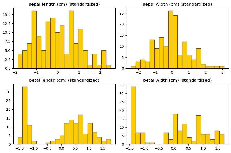
Figure1: Imagegeneratedbytheprovidedcode.

Readingtheplot/table: A erstandardization,eachfeaturecentersaroundzero withunitvariance.Thismakesgradientstepscomparableacrosscoordinatesand distancesmoremeaningfulacrossfeatures.

Min-MaxScalingwith MinMaxScaler

• Whatitdoes: linearlymapseachfeaturetoaboundedrange,typically [0, 1].

• Whentouse: algorithmsthatassumeboundedinputs(e.g.,someneuralnets/activationsetups),orwhenyouneedtopreservetheoriginaldistribution shapebutcompresstoaﬁxedinterval.

• Caveat: verysensitiveto outliers (minandmaxareextremepoints).

3 scaler_mm = MinMaxScaler(feature_range=(0,1)) 4 X_mm = pd.DataFrame(scaler_mm.fit_transform(X_iris), columns=cols)

5 6 #Showmin/maxafterscaling

7 mm_bounds = pd.DataFrame({ 8 "min_after": X_mm.min(), 9 "max_after": X_mm.max() 10 }).round(3) 11 display(mm_bounds) 1 from sklearn.preprocessing import

3 scaler_mm = MinMaxScaler(feature_range=(0,1)) 4 X_mm = pd.DataFrame(scaler_mm.fit_transform(X_iris), columns=cols) 5 6 #Showmin/maxafterscaling

7 mm_bounds = pd.DataFrame({ 8 "min_after": X_mm.min(), 9 "max_after": X_mm.max() 10 }).round(3) 11 display(mm_bounds) min_a er max_a er

1 #2Dscatterbeforevsafter(addsvalue:visualboundto [0,1])

2 fig, ax = plt.subplots(1,2, figsize=(10,4))

3 ax[0].scatter(X_iris[cols[0]], X_iris[cols[1]], s=12)

4 ax[0].set_title(f"Raw:{cols[0]}vs{cols[1]}")

5 ax[1].scatter(X_mm[cols[0]], X_mm[cols[1]], s=12)

6 ax[1].set_title(f"Min-Max:{cols[0]}vs{cols[1]}")

7 plt.tight_layout()

8 plt.show()

1 #2Dscatterbeforevsafter(addsvalue:visualboundto [0,1])

2 fig, ax = plt.subplots(1,2, figsize=(10,4))

3 ax[0].scatter(X_iris[cols[0]], X_iris[cols[1]], s =50, color = '#6b99a6ff')

4 ax[0].set_title(f"Raw:{cols[0]}vs{cols[1]}")

5 ax[1].scatter(X_mm[cols[0]], X_mm[cols[1]], s =50, color = '#6b99a6ff')

6 ax[1].set_title(f"Min-Max:{cols[0]}vs{cols[1]}") IbonMartínez-ArranzPage51

7 plt.tight_layout()

8 plt.show()

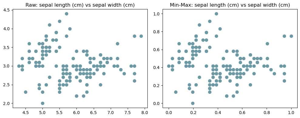
Figure2: Imagegeneratedbytheprovidedcode.

Readingtheplot/table: Allfeaturesaresqueezedinto[0,1].Relativepositionsare preserved,butoutlierscandominatethemapping.

RobustScalingwith RobustScaler

• Whatitdoes: centersusingthe median andscalesbythe interquartile range(IQR).

• Whentouse: datawith outliers orheavytails;keepsthebulkofthedistributioncomparablewithoutbeingdistortedbyextremes.

1 from sklearn.preprocessing import RobustScaler

3 #Createasyntheticfeaturewithclearoutlierstoshow thebenefit

4 rng = np.random.default_rng(7)

5 x_main = rng.normal(loc=50, scale=10, size=400)

6 x_out = rng.normal(loc=120, scale=5, size=10) # outliers 7 x = np.concatenate([x_main, x_out])

X_synth = pd.DataFrame({"feature": x})

X_std_s = pd.DataFrame(scaler_std_s.fit_transform(X_synth ), columns=["feature"])

X_rob = pd.DataFrame(scaler_rob.fit_transform(X_synth), columns=["feature"])

#Boxplots:standardvsrobust(addsvalue:robust reducesoutlierdistortion)

18 fig, ax = plt.subplots(1,2, figsize=(8,4))

19 ax[0].boxplot(X_std_s["feature"], vert=True) 20 ax[0].set_title("StandardScaler")

21 ax[1].boxplot(X_rob["feature"], vert=True) 22 ax[1].set_title("RobustScaler") 23 plt.tight_layout()

plt.show() 1 from sklearn.preprocessing import RobustScaler

3 #Createasyntheticfeaturewithclearoutlierstoshow thebenefit

4 rng = npy.random.default_rng(7)

5 x_main = rng.normal(loc=50, scale=10, size=400) 6 x_out = rng.normal(loc=120, scale=5, size=10) # outliers 7 x = npy.concatenate([x_main, x_out])

X_std_s = pd.DataFrame(scaler_std_s.fit_transform(X_synth ), columns=["feature"])

X_rob = pd.DataFrame(scaler_rob.fit_transform(X_synth), columns=["feature"])

17 #Boxplots:standardvsrobust(addsvalue:robust reducesoutlierdistortion)

18 fig, ax = plt.subplots(1,2, figsize=(8,4))

19 ax[0].boxplot(X_std_s["feature"], vert=True)

20 ax[0].set_title("StandardScaler")

21 ax[1].boxplot(X_rob["feature"], vert=True)

22 ax[1].set_title("RobustScaler")

23 plt.tight_layout()

24 plt.show()

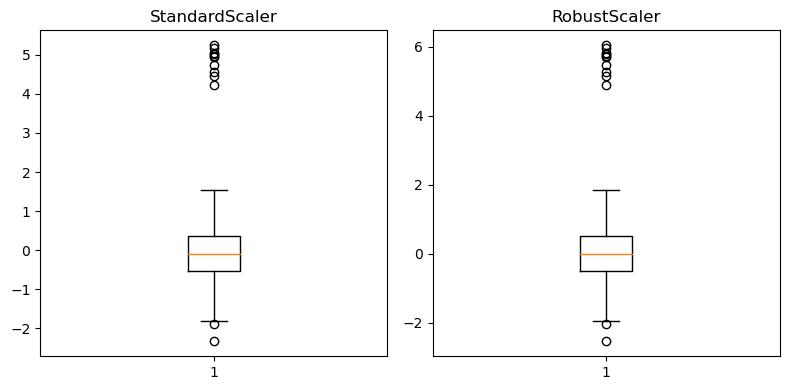
Figure3: Imagegeneratedbytheprovidedcode.

Readingtheplot: Robustscalingcompressesthecentralmasssimilarlyacross featureswhilepreventingafewextremevaluesfromstretchingthescale.

Comparingscalingmethodsonthesamedataset

Wequantifytheimpactona distance-basedmodel:k-NearestNeighbors(kNN) regressionontheCaliforniaHousingdataset.

Wecompare noscaling, StandardScaler,and MinMaxScaler usingcross-validated RMSE. (Wesubsampletokeepruntimereasonable.)

1 from sklearn.datasets import fetch_california_housing 2 from sklearn.model_selection import cross_val_score

from sklearn.neighbors import KNeighborsRegressor

from sklearn.pipeline import Pipeline

#Loaddata 7 housing = fetch_california_housing(as_frame=True) 8 X_h = housing.frame.drop(columns=["MedHouseVal"])

y_h = housing.frame["MedHouseVal"]

#Subsampletospeedup(adjustasneeded) 12 sample = X_h.sample(n=5000, random_state=42)

target = y_h.loc[sample.index]

def rmse(scores):

return np.sqrt(-scores.mean())

pipelines ={ 19 "NoScaling": Pipeline([("model", KNeighborsRegressor (n_neighbors=5))]),

20 "StandardScaler": Pipeline([("scaler", StandardScaler ()),("model", KNeighborsRegressor(n_neighbors=5) )]),

21 "MinMaxScaler": Pipeline([("scaler", MinMaxScaler()), ("model", KNeighborsRegressor(n_neighbors=5))]),

}

results ={} 25 for name, pipe in pipelines.items(): 26 scores = cross_val_score(pipe, sample, target, scoring="neg_mean_squared_error", cv=5, n_jobs

27 results[name]=[rmse(scores)]

29 results_df = pd.DataFrame(results).T 30 results_df.columns =["RMSE"]

31 results_df = results_df.sort_values("RMSE")

33 #Barplot(addsvalue:quickvisualcomparison)

34 fig, ax = plt.subplots(figsize=(6,4))

35 ax.bar(results_df.index, results_df["RMSE"])

36 ax.set_ylabel("RMSE(lowerisbetter)")

37 ax.set_title("kNNRegression-EffectofScaling") 38 plt.tight_layout()

39 plt.show()

1 from sklearn.datasets import fetch_california_housing 2 from sklearn.model_selection import cross_val_score 3 from sklearn.neighbors import KNeighborsRegressor 4 from sklearn.pipeline import Pipeline

#Loaddata 7 housing = fetch_california_housing(as_frame=True)

8 X_h = housing.frame.drop(columns=["MedHouseVal"])

y_h = housing.frame["MedHouseVal"]

#Subsampletospeedup(adjustasneeded)

sample = X_h.sample(n=5000, random_state=42)

target = y_h.loc[sample.index]

def rmse(scores):

return npy.sqrt(-scores.mean())

pipelines ={ 19 "NoScaling": Pipeline([("model", KNeighborsRegressor (n_neighbors=5))]),

20 "StandardScaler": Pipeline([("scaler", StandardScaler ()),("model", KNeighborsRegressor(n_neighbors=5) )]),

21 "MinMaxScaler": Pipeline([("scaler", MinMaxScaler()), ("model", KNeighborsRegressor(n_neighbors=5))]), 22 }

EssentialGuidetoFeatureEngineering

24 results ={}

25 for name, pipe in pipelines.items(): 26 scores = cross_val_score(pipe, sample, target, scoring="neg_mean_squared_error", cv=5, n_jobs =-1)

27 results[name]=[rmse(scores)] 28

29 results_df = pd.DataFrame(results).T

30 results_df.columns =["RMSE"]

31 results_df = results_df.sort_values("RMSE")

33 #Barplot(addsvalue:quickvisualcomparison)

34 fig, ax = plt.subplots(figsize=(6,4))

35 ax.bar(results_df.index, results_df["RMSE"], color =['# b7d3dbff' , '#6b99a6ff' , '#3a6674ff'])

36 ax.set_ylabel("RMSE(lowerisbetter)")

37 ax.set_title("kNNRegression-EffectofScaling")

38 plt.tight_layout()

39 plt.show()

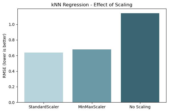
Figure4: Imagegeneratedbytheprovidedcode.

Interpretingthenumbers: Distance-basedmodelstypicallybeneﬁtfromscaling. Whichscalerwinscandependonfeaturedistributions;standardizationisarobust default,MinMaxcanhelpifyouwantallfeaturesinaﬁxedrange.

Practicaltips:essentialvsoptional

• Essential/highlyrecommended

– kNN,K-Means,SVMwithkernels,PCA/UMAP/t-SNE,Linear/LogisticRegressionwithregularization,NeuralNetworks.

– Mixed-unitfeatures(e.g., income inthousandsvs rooms count)almostalwaysneedscaling.

• Usefulbutsituational

– Whenfeatureshaveverydi erentvariances;standardizationevenstheir inﬂuence.

– Whenoptimizationisunstableorslowtoconverge.

• Usuallyoptional

– Tree-basedmethods(RandomForests,GradientBoostedTrees,XGBoost/LightGBM/CatBoost).

– Modelsthatdonotusedistancesorgradientsinwayssensitivetoscale.

Ruleofthumb: startwith StandardScaler;consider RobustScaler ifoutliers dominate;use MinMaxScaler whenaboundedrangeisrequiredorwhenfeeding intomethodsexpecting[0,1].

Whatcomesnext

Wehavethecorescalersunderourbelt.Nextchapter,we’lllookat transformations totameskeweddistributions: logtransforms, Box-Cox,and Yeo-Johnson,and howtocombinetheminside pipelines.

TransformingVariables

Detectingskewnessandchoosingatransformation

Manyreal-worldfeaturesare skewed (longtails).Skewnesscanharmmodelsthat assumenear-normalinputsorusedistances/gradients.Typicalﬁxes:

• Logtransform:forstrictlypositive,right-skewedvariables.

• Box-Cox / Yeo-Johnson:learnpowerparameters;Box-Coxneedsstrictly positivevalues;Yeo-Johnsonhandleszero/negative.

• Quantiletransforms:reshapedistributionsto normal or uniform viarank mapping.

• Binarization:converttoindicatorfeatureswhenonlyathresholdmatters.

We’ll:

1)measureskewness, 2)applyseveraltransforms, 3)comparebefore/a eronrepresentativefeatures.

1 import pandasaspd

2 import matplotlib.pyplotasplt 3 4 from sklearn.datasets import fetch_california_housing 5 from sklearn.preprocessing import FunctionTransformer, PowerTransformer, QuantileTransformer, Binarizer

7 #LoadCaliforniaHousing(allnumeric,severalskewed)

8 cal = fetch_california_housing(as_frame=True)

Latitude

HouseAge

Logtransformationsforskeweddata

Whentouse: strictlypositive,right-skewedfeatures(counts,incomes,areas).We willuse npy.log1p(x) (log(1+x))whichisstablenearzero.

Wewillillustrateontwocommonlyskewedfeaturesfromthisdataset:

• MedInc (medianincome)

• Population

Wewillverifypositivityandthencomparehistogramsbefore/a er.

1 def plot_hist_pair(series_raw, series_tx, title_raw, title_tx):

2 fig, axes = plt.subplots(1,2, figsize=(10,4))

axes[0].hist(series_raw, bins =30, color = "#FECB00" , edgecolor = '0.3',) 4 axes[0].set_title(title_raw)

5 axes[1].hist(series_tx, bins =30, color = "#FECB00", edgecolor = '0.3',)

6 axes[1].set_title(title_tx) 7 plt.tight_layout() 8 plt.show()

#Choosetwofeatures 11 feat_log_candidates =["MedInc", "Population"] 12 for feat in feat_log_candidates: 13 s = X[feat].dropna() 14 #Ensurestrictlypositiveforlog 15 s_pos = s[s >0] 16 s_log = npy.log1p(s_pos)

18 plot_hist_pair( 19 s_pos, s_log, 20 f"{feat}(raw)", 21 f"{feat}(log1p)"

)

24 #Skewnesscomparisontableforselectedfeatures

25 log_rows =[]

26 for feat in feat_log_candidates:

27 s = X[feat].dropna()

28 s_pos = s[s >0]

29 s_log = npy.log1p(s_pos)

30 log_rows.append({ 31 "feature": feat, 32 "skew_raw": float(s_pos.skew()),

33 "skew_log1p": float(pd.Series(s_log).skew()), 34 })

1 def plot_hist_pair(series_raw, series_tx, title_raw, title_tx):

2 fig, axes = plt.subplots(1,2, figsize=(10,4))

3 axes[0].hist(series_raw, bins =30, color = "#FECB00" , edgecolor = '0.3',)

4 axes[0].set_title(title_raw)

5 axes[1].hist(series_tx, bins =30, color = "#FECB00", edgecolor = '0.3',)

axes[1].set_title(title_tx)

plt.tight_layout()

plt.show()

#Choosetwofeatures

feat_log_candidates =["MedInc", "Population"]

for feat in feat_log_candidates:

s = X[feat].dropna()

s_pos = s[s >0]

s_log = npy.log1p(s_pos)

plot_hist_pair(

s_pos, s_log,

f"{feat}(raw)",

f"{feat}(log1p)"

)

#Skewnesscomparisontableforselectedfeatures 25 log_rows =[]

for feat in feat_log_candidates:

s = X[feat].dropna()

s_pos = s[s >0]

s_log = npy.log1p(s_pos) 30 log_rows.append({ 31 "feature": feat, 32 "skew_raw": float(s_pos.skew()), 33 "skew_log1p": float(pd.Series(s_log).skew()), 34 })

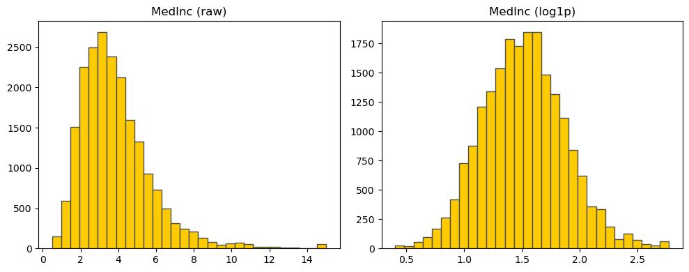
Figure1: Imagegeneratedbytheprovidedcode.

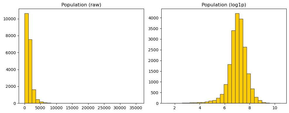
Figure2: Imagegeneratedbytheprovidedcode.

Readingtheplots/table: Thelogtransformtypicallyreducesrightskewnessand compresseslongtails,makinggradientsanddistancesmorestable.

Box-CoxandYeo-Johnsonwith PowerTransformer

PowerTransformer estimatesapowerparameterperfeaturetomakethedata moreGaussian-like.

• Box-Cox worksonlyfor strictlypositive data.

• Yeo-Johnson worksfor zero/negative aswellandiso enasafedefault. Wewillapplybothwherepossibleandcompareskewnessreductions. 1 from sklearn.compose import ColumnTransformer

#IdentifystrictlypositivecolumnsforBox-Cox(min> 0) 4 positive_cols =[c for c in cols if (X[c]>0).all()] 5 non_positive_cols =[c for c in cols if c notin positive_cols]

7 pt_boxcox = PowerTransformer(method="box-cox", standardize=True) 8 pt_yeojohn = PowerTransformer(method="yeo-johnson", standardize=True)

#Fit/transformseparatecopiesforclarity

X_box = X[positive_cols].copy()

X_box_tx = pd.DataFrame(pt_boxcox.fit_transform(X_box), columns=positive_cols, index=X_box.index)

X_yj = X.copy() 15 X_yj_tx = pd.DataFrame(pt_yeojohn.fit_transform(X_yj), columns=cols, index=X.index)

17 #Skewnesssummaries(medianacrossfeaturesasacompact signal) 18 summary_skew = pd.DataFrame({

"median_skew_raw":[X.skew().median()],

"median_skew_boxcox_(pos_only)":[X_box_tx.skew(). median() if len(positive_cols) else npy.nan], 21 "median_skew_yeojohnson":[X_yj_tx.skew().median()] 22 }).round(3)

23 display(summary_skew)

25 #VisualexampleonMedIncwithYeo-Johnson(addsvalue ifdifferentfromlog) 26 feat = "MedInc"

s_raw = X[feat]

s_yj = X_yj_tx[feat]

29 plot_hist_pair(s_raw, s_yj, f"{feat}(raw)", f"{feat}( Yeo-Johnson)", "fig_medinc_yj_hist.png")

3 #IdentifystrictlypositivecolumnsforBox-Cox(min> 0)

4 positive_cols =[c for c in cols if (X[c]>0).all()] 5 non_positive_cols =[c for c in cols if c notin positive_cols]

7 pt_boxcox = PowerTransformer(method="box-cox", standardize=True)

8 pt_yeojohn = PowerTransformer(method="yeo-johnson", standardize=True)

X_box = X[positive_cols].copy()

X_box_tx = pd.DataFrame(pt_boxcox.fit_transform(X_box), columns=positive_cols, index=X_box.index)

X_yj = X.copy()

X_yj_tx = pd.DataFrame(pt_yeojohn.fit_transform(X_yj), columns=cols, index=X.index)

#Skewnesssummaries(medianacrossfeaturesasacompact signal)

18 summary_skew = pd.DataFrame({ 19 "median_skew_raw":[X.skew().median()], 20 "median_skew_boxcox_(pos_only)":[X_box_tx.skew(). median() if len(positive_cols) else npy.nan],

"median_skew_yeojohnson":[X_yj_tx.skew().median()] 22 }).round(3)

24 #VisualexampleonMedIncwithYeo-Johnson(addsvalue ifdifferentfromlog)

25 feat = "MedInc"

26 s_raw = X[feat]

27 s_yj = X_yj_tx[feat]

28 plot_hist_pair(s_raw, s_yj, f"{feat}(raw)", f"{feat}( Yeo-Johnson)",)

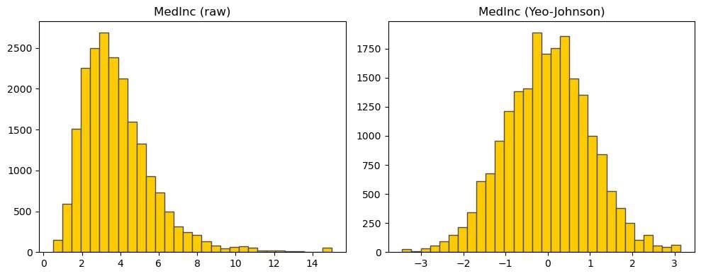
Figure3: Imagegeneratedbytheprovidedcode.

Interpretation: BothBox-CoxandYeo-Johnsonusuallyreduceskewness.YeoJohnsonismoreﬂexibleandavoidsthe“strictlypositive”constraint.

Quantiletransformationsfornon-Gaussian distributions

QuantileTransformer mapsvaluestotheirempiricalquantilesandthentoatarget distribution:

• output_distribution="normal" → approximatelystandard normal.

• output_distribution="uniform" → approximatelyuniformon[0, 1].

Thiscandramaticallystabilizehighlynon-Gaussianfeatures,atthecostofnonlineardistortions.

1 qt_norm = QuantileTransformer(output_distribution="normal " , random_state=42)

2 qt_unif = QuantileTransformer(output_distribution=" uniform", random_state=42)

4 feat = "Population" #typicallyheavy-tailed

5 s = X[feat].values.reshape(-1,1) 6

7 s_norm = qt_norm.fit_transform(s).ravel()

8 s_unif = qt_unif.fit_transform(s).ravel() 9

10 #Histogramstoshowtargetdistributions

11 fig, axes = plt.subplots(1,3, figsize=(12,4))

12 axes[0].hist(s.ravel(), bins=30)

13 axes[0].set_title(f"{feat}(raw)")

14 axes[1].hist(s_norm, bins=30)

15 axes[1].set_title(f"{feat}(Quantile->Normal)")

16 axes[2].hist(s_unif, bins=30)

17 axes[2].set_title(f"{feat}(Quantile->Uniform)")

18 plt.tight_layout()

19 plt.show()

1 qt_norm = QuantileTransformer(output_distribution="normal " , random_state=42)

2 qt_unif = QuantileTransformer(output_distribution=" uniform", random_state=42)

4 feat = "Population" #typicallyheavy-tailed

5 s = X[feat].values.reshape(-1,1) 6

7 s_norm = qt_norm.fit_transform(s).ravel()

8 s_unif = qt_unif.fit_transform(s).ravel() 9

#Histogramstoshowtargetdistributions

11 fig, axes = plt.subplots(1,3, figsize=(12,4))

12 axes[0].hist(s.ravel(), bins=30, color = "#FECB00", edgecolor = '0.3',)

13 axes[0].set_title(f"{feat}(raw)")

14 axes[1].hist(s_norm, bins=30, color = "#FECB00", edgecolor = '0.3',)

15 axes[1].set_title(f"{feat}(Quantile->Normal)")

16 axes[2].hist(s_unif, bins=30, color = "#FECB00", edgecolor = '0.3',)

17 axes[2].set_title(f"{feat}(Quantile->Uniform)")

18 plt.tight_layout()

19 plt.show()

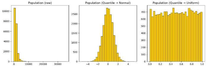
Figure4: Imagegeneratedbytheprovidedcode.

Trade-o : Quantiletransformscangreatlyhelpalgorithmsneedingnear-Gaussian inputsbutmaywarprelationships.Considerapplyingthemwithin pipelines and validatetheirimpactonyourmetrics.

Binarizationwith Binarizer

Binarizer convertsanumericfeatureintoabinaryindicatorusingathreshold. Useitwhena decisionboundary (e.g.,above/belowmedianoradomain-speciﬁc cuto )carriesmostofthepredictivesignal.

bin_tx = Binarizer(threshold=threshold) #>threshold becomes1.0 5 medinc_bin = bin_tx.fit_transform(X[["MedInc"]]).ravel()

#Simplebefore/aftervisualization(addsvalue:shows thediscretization)

12 fig, axes = plt.subplots(1,2, figsize=(9,4))

13 axes[0].hist(X["MedInc"], bins=30, color = "#FECB00", edgecolor = '0.3',)

14 axes[0].set_title("MedInc(raw)")

15 axes[1].hist(medinc_bin, bins=2, color = "#FECB00", edgecolor = '0.3',)

16 axes[1].set_xticks([0,1])

17 axes[1].set_title("MedInc(binarized)")

18 plt.tight_layout()

19 plt.show()

#Showproportionof1s 8 prop_high = medinc_bin.mean()

print(f"Thresholdused:{threshold:.3f};shareabove threshold:{prop_high:.2%}")

12 fig, axes = plt.subplots(1,2, figsize=(9,4))

13 axes[0].hist(X["MedInc"], bins=30, color = "#FECB00", edgecolor = '0.3',)

14 axes[0].set_title("MedInc(raw)")

15 axes[1].hist(medinc_bin, bins=2, color = "#FECB00", edgecolor = '0.3',)

16 axes[1].set_xticks([0,1])

17 axes[1].set_title("MedInc(binarized)")

18 plt.tight_layout()

19 plt.show()

1 Thresholdused:3.535; shareabovethreshold:50.00%

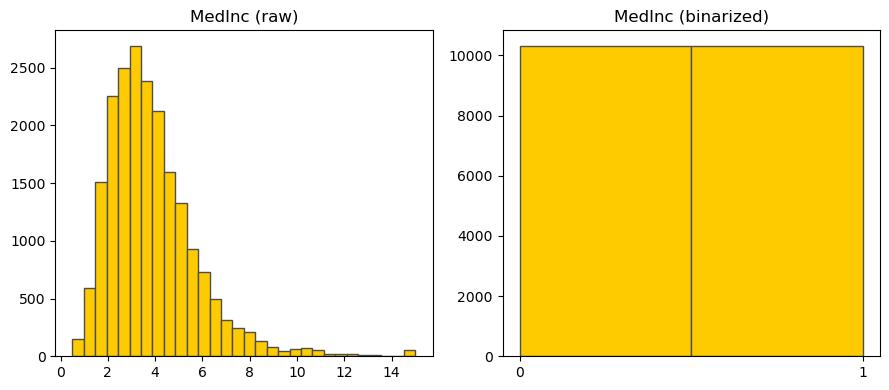
Figure5: Imagegeneratedbytheprovidedcode.

Caution: Binarizationdiscardswithin-binvariation.Itcanbepowerfulforrulelikesignalsbutmayreduceinformationformodelsthatbeneﬁtfromcontinuous structure.

Combiningtransformationswithpipelines

Wewill:

• Apply Yeo-Johnson toskewedfeatures,

• Leaveapproximatelysymmetricfeaturesas-is(orstandardize),

• Adda binarized versionof MedInc viaaseparatepipelinebranch,

• Trainasimple Ridge regressorontheCaliforniaHousingtargettoillustrate end-to-endusage.

WewillcompareRMSEwithandwithouttransformations.

1 from sklearn.pipeline import Pipeline 2 from sklearn.compose import ColumnTransformer 3 from sklearn.linear_model import Ridge

from sklearn.model_selection import cross_val_score

6 target = cal.frame["MedHouseVal"]

8 #Heuristic:markskewedif|skew|>=1.0 9 skews = X.skew().abs() 10 skewed_cols = skews[skews >=1.0].index.tolist()

other_cols =[c for c in cols if c notin skewed_cols]

13 #Pipelinesforbranches 14 yj_pipe = Pipeline(steps=[

("yeojohn", PowerTransformer(method="yeo-johnson", standardize=True))

])

#"Passthrough"forothercolumns(youcouldadd StandardScalerifdesired) 19 pass_pipe = "passthrough"

21 #BinarizedMedIncasanextrafeature(single-column pipeline)

22 bin_col =["MedInc"] 23 bin_threshold = float(X["MedInc"].median()) 24 bin_pipe = Pipeline(steps=[

EssentialGuidetoFeatureEngineering

25 ("bin", Binarizer(threshold=bin_threshold))

])

28 #ColumnTransformercombiningbranches(note:binarized MedIncwillappearalongsideraw/otherfeatures)

29 preprocessor = ColumnTransformer(

transformers=[

31 ("yj", yj_pipe, skewed_cols),

("other", pass_pipe, other_cols), 33 ("medinc_bin", bin_pipe, bin_col),

remainder="drop",

verbose_feature_names_out=False

)

39 model = Ridge(alpha=1.0, random_state=42)

41 pipe_tx = Pipeline(steps=[ 42 ("prep", preprocessor),

43 ("model", model)

])

46 pipe_raw = Pipeline(steps=[

47 ("model", Ridge(alpha=1.0, random_state=42)) 48 ])

50 def rmse(cv_scores):

51 return npy.sqrt(-cv_scores.mean())

53 scores_tx = cross_val_score(pipe_tx, X, target, scoring=" neg_mean_squared_error", cv=5, n_jobs=-1)

54 scores_raw = cross_val_score(pipe_raw, X, target, scoring ="neg_mean_squared_error", cv=5, n_jobs=-1)

56 print("RMSE(notransforms):", rmse(scores_raw))

57 print("RMSE(withtransforms):", rmse(scores_tx))

1 from sklearn.pipeline import Pipeline

2 from sklearn.compose import ColumnTransformer 3 from sklearn.linear_model import Ridge 4 from sklearn.model_selection import cross_val_score

#Heuristic:markskewedif|skew|>=1.0

skews = X.skew().abs()

skewed_cols = skews[skews >=1.0].index.tolist()

other_cols =[c for c in cols if c notin skewed_cols]

yj_pipe = Pipeline(steps=[

("yeojohn", PowerTransformer(method="yeo-johnson", standardize=True))

#"Passthrough"forothercolumns(youcouldadd StandardScalerifdesired)

pass_pipe = "passthrough"

#BinarizedMedIncasanextrafeature(single-column pipeline)

bin_col =["MedInc"]

bin_threshold = float(X["MedInc"].median())

bin_pipe = Pipeline(steps=[

("bin", Binarizer(threshold=bin_threshold))

])

#ColumnTransformercombiningbranches(note:binarized MedIncwillappearalongsideraw/otherfeatures)

preprocessor = ColumnTransformer(

transformers=[

("yj", yj_pipe, skewed_cols),

("other", pass_pipe, other_cols),

("medinc_bin", bin_pipe, bin_col),

remainder="drop",

verbose_feature_names_out=False

)

model = Ridge(alpha=1.0, random_state=42)

pipe_tx = Pipeline(steps=[ Page76IbonMartínez-Arranz

EssentialGuidetoFeatureEngineering

42 ("prep", preprocessor),

43 ("model", model) 44 ]) 45

46 pipe_raw = Pipeline(steps=[

47 ("model", Ridge(alpha=1.0, random_state=42))

48 ])

50 def rmse(cv_scores):

51 return npy.sqrt(-cv_scores.mean())

53 scores_tx = cross_val_score(pipe_tx, X, target, scoring=" neg_mean_squared_error", cv=5, n_jobs=-1)

54 scores_raw = cross_val_score(pipe_raw, X, target, scoring ="neg_mean_squared_error", cv=5, n_jobs=-1)

56 print("RMSE(notransforms):", rmse(scores_raw))

57 print("RMSE(withtransforms):", rmse(scores_tx))

1 RMSE (notransforms):0.7471805175916729

2 RMSE (withtransforms):0.7315995010450792

Howtoreadthecomparison: IfRMSEimproveswithtransformations,thepreprocessingmeaningfullystabilizedthefeaturespaceforthismodel.Ifnot,revisitwhich columnsyoutransformandconsiderStandardScalerfornon-skewedcolumns.

Summary

• Log isasimple,e ectiveﬁxforpositive,right-skeweddata.

• PowerTransformer (Box-Cox/Yeo-Johnson)learnspowerparameters;YeoJohnsonismoregeneral.

• QuantileTransformer canenforcenear-normaloruniformoutputsbutis highlynon-linear;validateitsimpact.

• Binarizer isusefulwhenathresholdcarriesmostofthesignal.

• Combinethesestepsusing pipelines sotrainingandinferencestayconsistent IbonMartínez-ArranzPage77

andreproducible.

FeatureGeneration

Creatinginteractionfeatures

(PolynomialFeatures)

Interactionfeatures capturemultiplicativerelationshipsbetweenvariables(e.g., x1 * x2).

Theyallow linear modelstoapproximatenon-linearboundarieswithoutchanging themodelclass.

We’llillustratewithtwonumericalpredictorsfromCaliforniaHousingandshow howtocreate:

• Interactionsonly (nosquares),

• Full polynomial termsuptodegree2(includingsquaresandinteractions).

Caution: Polynomialexpansioncanexplodedimensionality—validatewithcrossvalidationandregularization.

1 import numpyasnpy

2 import pandasaspd

3 import matplotlib.pyplotasplt

5 from sklearn.datasets import fetch_california_housing

6 from sklearn.preprocessing import PolynomialFeatures

8 cal = fetch_california_housing(as_frame=True)

9 Xh = cal.frame.drop(columns=["MedHouseVal"])

10 y = cal.frame["MedHouseVal"]

= PolynomialFeatures(degree=2, include_bias= False, interaction_only=True)

= pd.DataFrame(poly_int.fit_transform(X_pair), columns=poly_int.get_feature_names_out(num_pair))

= PolynomialFeatures(degree=2, include_bias= False, interaction_only=False)

= pd.DataFrame(poly_full.fit_transform(X_pair), columns=poly_full.get_feature_names_out(num_pair))

print("Interaction-onlycolumns:", X_int.columns.tolist() )

print("Quadraticcolumns:", X_quad.columns.tolist())

5 from sklearn.datasets import fetch_california_housing

from sklearn.preprocessing import PolynomialFeatures

cal = fetch_california_housing(as_frame=True)

Xh = cal.frame.drop(columns=["MedHouseVal"])

= cal.frame["MedHouseVal"]

= PolynomialFeatures(degree=2, include_bias= False, interaction_only=True)

X_int = pd.DataFrame(poly_int.fit_transform(X_pair), columns=poly_int.get_feature_names_out(num_pair))

EssentialGuidetoFeatureEngineering

19 #Fullquadratic(squares+interactions)

20 poly_full = PolynomialFeatures(degree=2, include_bias= False, interaction_only=False)

21 X_quad = pd.DataFrame(poly_full.fit_transform(X_pair), columns=poly_full.get_feature_names_out(num_pair))

23 print("Interaction-onlycolumns:", X_int.columns.tolist() )

24 print("Quadraticcolumns:", X_quad.columns.tolist())

25 display(X_int.head())

26 display(X_quad.head())

1 Interaction-onlycolumns:['MedInc' , 'HouseAge' , 'MedInc HouseAge']

2 Quadraticcolumns:['MedInc' , 'HouseAge' , 'MedInc^2' , ' MedIncHouseAge' , 'HouseAge^2']

Whenithelps: Iftarget ≈ smoothfunctionofinputswithcross-e ects(e.g.,income × houseage),interactionsletlinearmodelsweightthosee ectsdirectly.

Featurecrosses:combiningcategoricalfeatures

Featurecrosses joincategoriestocapture co-occurrencepatterns (e.g., sex × class inTitanic).

Twocommonapproaches:

1) Manualcrossinpandas,thenone-hotencode.

2) OneHot → PolynomialFeatures(interaction_only=True):createinteractions a er one-hot(watchoutfordimensionality).

We’lldemonstratethemanualrouteforclarityandcontrol.

1 import seabornassns

2 import numpyasnpy 3 import pandasaspd

4 from sklearn.compose import ColumnTransformer

5 from sklearn.preprocessing import OneHotEncoder 6 from sklearn.linear_model import LogisticRegression 7 from sklearn.pipeline import Pipeline

8 from sklearn.model_selection import cross_val_score 9 from sklearn.impute import SimpleImputer

titanic = sns.load_dataset("titanic").copy()

X = titanic[["sex", "class", "embarked", "age", "fare"]]

y = titanic["survived"]

#Manualcrossofcategoricalfeatures 16 X = X.assign(sex_class=X["sex"].astype(str)+ "_" + X[" class"].astype(str))

#Columngroups 19 nominal =["sex", "embarked", "sex_class"]

numeric =["age", "fare"]

#OneHotEncodercompatibilityshim(sklearn>=1.2uses sparse_output) 23 try:

EssentialGuidetoFeatureEngineering

24 ohe = OneHotEncoder(handle_unknown="ignore", sparse_output=False) 25 except TypeError:

ohe = OneHotEncoder(handle_unknown="ignore", sparse= False)

#Buildpreprocessing:imputefirst(train-onlyinsideCV ),thenencode/passthrough 29 pre = ColumnTransformer( 30 transformers=[

#Nominalfeatures:imputemostfrequentcategory ,thenone-hotencode

("nominal", Pipeline([

("imputer", SimpleImputer(strategy=" most_frequent")),

("ohe", ohe),

]), nominal),

#Numericfeatures:imputemedian(robustto outliers)

38 ("numeric", Pipeline([

("imputer", SimpleImputer(strategy="median")) , 40 ]), numeric),

verbose_feature_names_out=False

)

45 #End-to-endpipeline:preprocessing+classifier 46 pipe = Pipeline([

("prep", pre),

("clf", LogisticRegression(max_iter=1000))

])

51 #Cross-validatedaccuracy

52 scores = cross_val_score(pipe, X, y, cv=5, scoring=" accuracy", n_jobs=-1)

53 print("Cross-validatedaccuracy(withcrossedfeature+ imputation):", scores.mean().round(3))

from sklearn.linear_model import

from sklearn.pipeline import Pipeline

from sklearn.model_selection import cross_val_score

from sklearn.impute import SimpleImputer

titanic = sns.load_dataset("titanic").copy()

= titanic[["sex", "class", "embarked", "age", "fare"]]

X = X.assign(sex_class=X["sex"].astype(str)+ "_" + X[" class"].astype(str))

nominal =["sex", "embarked", "sex_class"]

numeric =["age", "fare"]

#OneHotEncodercompatibilityshim(sklearn>=1.2uses sparse_output) 23 try:

ohe = OneHotEncoder(handle_unknown="ignore", sparse_output=False)

except TypeError:

ohe = OneHotEncoder(handle_unknown="ignore", sparse= False)

#Buildpreprocessing:imputefirst(train-onlyinsideCV ),thenencode/passthrough

pre = ColumnTransformer(

transformers=[

#Nominalfeatures:imputemostfrequentcategory ,thenone-hotencode

("nominal", Pipeline([

("imputer", SimpleImputer(strategy=" most_frequent")),

("ohe", ohe),

]), nominal),

37 #Numericfeatures:imputemedian(robustto outliers)

38 ("numeric", Pipeline([ 39 ("imputer", SimpleImputer(strategy="median")) , 40 ]), numeric),

], 42 verbose_feature_names_out=False

)

45 #End-to-endpipeline:preprocessing+classifier 46 pipe = Pipeline([

("prep", pre), 48 ("clf", LogisticRegression(max_iter=1000))

])

51 #Cross-validatedaccuracy

52 scores = cross_val_score(pipe, X, y, cv=5, scoring=" accuracy", n_jobs=-1)

53 print("Cross-validatedaccuracy(withcrossedfeature+ imputation):", scores.mean().round(3))

1 Cross-validatedaccuracy (withcrossedfeature + imputation):0.797

Tip: Crossesarepowerfulwhencertainpairsofcategoriesbehavedi erentlythan eachonealone(e.g., male in First classvs Third class).

Extractingdate/timefeatures

Timestampsencode periodic and calendar signals(seasonality,weekdayvsweekend,rushhours).

Typicalextractions:

• year, month, day, weekday, hour, weekofyear.

• Cyclicalencodings forperiodicvariables(e.g.,hour-of-day)using sin/cos.

BelowwecreateasmallexampleDataFramewithtimestampsandextractinformativefeatures.

5 #Syntheticeventtimestamps(hourlyfor~2weeks)

6 ts = pd.date_range("2023-05-01", periods=24*14, freq="H") 7 events = pd.DataFrame({ 8 "timestamp": ts,

"value": npy.random.default_rng(0).normal(loc=0, scale=1, size=len(ts))

#Basiccalendarfeatures

events["year"]= events["timestamp"].dt.year

events["month"]= events["timestamp"].dt.month 15 events["day"]= events["timestamp"].dt.day 16 events["weekday"]= events["timestamp"].dt.weekday #0= Mon

events["hour"]= events["timestamp"].dt.hour 18 events["is_weekend"]= events["weekday"].isin([5,6]). astype(int)

20 #Cyclicalencodingsforhour-of-day 21 events["hour_sin"]= npy.sin(2*npy.pi*events["hour"]/24) 22 events["hour_cos"]= npy.cos(2*npy.pi*events["hour"]/24)

display(events.head())

#(Addsvalue)Quickweekdaycountplottoshowextracted structure 27 weekday_counts = events["weekday"].value_counts(). sort_index()

28 plt.figure(figsize=(5,3))

29 plt.bar(["Mon","Tue","Wed","Thu","Fri","Sat","Sun"], weekday_counts)

30 plt.title("Eventcountsbyweekday") 31 plt.tight_layout()

32 plt.savefig("fig_events_weekday_counts.png", dpi=150,

5 #Syntheticeventtimestamps(hourlyfor~2weeks)

6 ts = pd.date_range("2023-05-01", periods=24*14, freq="H")

7 events = pd.DataFrame({ 8 "timestamp": ts,

"value": npy.random.default_rng(0).normal(loc=0, scale=1, size=len(ts))

#Basiccalendarfeatures

events["year"]= events["timestamp"].dt.year

events["month"]= events["timestamp"].dt.month

events["day"]= events["timestamp"].dt.day 16 events["weekday"]= events["timestamp"].dt.weekday #0= Mon

events["hour"]= events["timestamp"].dt.hour 18 events["is_weekend"]= events["weekday"].isin([5,6]). astype(int)

20 #Cyclicalencodingsforhour-of-day 21 events["hour_sin"]= npy.sin(2*npy.pi*events["hour"]/24) 22 events["hour_cos"]= npy.cos(2*npy.pi*events["hour"]/24)

24 display(events.head())

26 #(Addsvalue)Quickweekdaycountplottoshowextracted structure

27 weekday_counts = events["weekday"].value_counts(). sort_index()

28 plt.figure(figsize=(5,3))

29 plt.bar(["Mon","Tue","Wed","Thu","Fri","Sat","Sun"], weekday_counts)

30 plt.title("Eventcountsbyweekday")

31 plt.tight_layout()

32 plt.show()

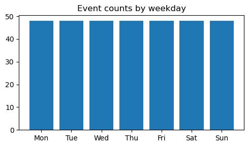
Figure1: Imagegeneratedbytheprovidedcode.

Whycyclicalfeatures? 23:00 and 00:00 areadjacentintimebutfarasintegers. Sine/cosinepreservecircularadjacencyformodelsthatreadnumbersliterally.

Textpreprocessingbasics:Bag-of-WordsandTF-IDF

Forshorttexts,twofoundations:

• Bag-of-Words(CountVectorizer):countstokenoccurrencesperdocument.

• TF-IDF(TﬁdfVectorizer):down-weightsubiquitoustokens,up-weightsdistinctiveones.

We’lluseatinycorpusandinspectthetop-weightedterms.

cv = CountVectorizer(stop_words="english")

X_bow = cv.fit_transform(corpus)

vocab = npy.array(cv.get_feature_names_out())

print("BOWshape:", X_bow.shape)

tfidf = TfidfVectorizer(stop_words="english")

X_tfidf = tfidf.fit_transform(corpus)

terms = npy.array(tfidf.get_feature_names_out())

#Showtop-5termsbyweightforeachdoc 23 for i, doc in enumerate(corpus):

row = X_tfidf.getrow(i).toarray().ravel() 25 top_idx = row.argsort()[-5:][::-1]

print(f"\nDoc{i}:", doc) 27 print("Topterms:", terms[top_idx].tolist(), "weights :", row[top_idx].round(3).tolist())

"Goodfeatureshelpsimplemodelscompete",

"Pipelineskeeppreprocessingreproducible",

12 cv = CountVectorizer(stop_words="english") 13 X_bow = cv.fit_transform(corpus) 14 vocab = npy.array(cv.get_feature_names_out()) 15 print("BOWshape:", X_bow.shape)

#TF-IDF

18 tfidf = TfidfVectorizer(stop_words="english")

19 X_tfidf = tfidf.fit_transform(corpus)

20 terms = npy.array(tfidf.get_feature_names_out())

22 #Showtop-5termsbyweightforeachdoc

23 for i, doc in enumerate(corpus):

24 row = X_tfidf.getrow(i).toarray().ravel()

25 top_idx = row.argsort()[-5:][::-1]

26 print(f"\nDoc{i}:", doc)

27 print("Topterms:", terms[top_idx].tolist(), "weights :", row[top_idx].round(3).tolist()) 1 BOWshape:(4,18)

3 Doc 0: Featureengineeringturnsdataintosignal 4 Topterms:['turns' , 'signal' , 'engineering' , 'data' , ' feature'] weights:[0.447,0.447,0.447,0.447, 0.447]

6 Doc 1: Goodfeatureshelpsimplemodelscompete

Topterms:['help' , 'simple' , 'features' , 'compete' , ' models'] weights:[0.408,0.408,0.408,0.408,0.408]

9 Doc 2: Pipelineskeeppreprocessingreproducible 10 Topterms:['preprocessing' , 'reproducible' , 'pipelines' , 'turns' , 'steps'] weights:[0.577,0.577,0.577, 0.0,0.0]

12 Doc 3: Scalingandencodingareessentialsteps 13 Topterms:['steps' , 'scaling' , 'encoding' , 'essential' , 'turns'] weights:[0.5,0.5,0.5,0.5,0.0]

Guidance: Forrealprojects,addtokenization/normalization(lowercasing,stem-

ming/lemmatization),n-grams,charactermodelsformisspellings,ordomainvocabularies.

Domain-drivenfeatures(CaliforniaHousing)

Domainknowledgeo enbeatsblindexpansion.Examplesforthisdataset:

• Bedroomsratio: AveBedrms / AveRooms (howmanybedroomsper room).

• Roomsperoccupant: AveRooms / AveOccup (spaceperperson).

• Incomeperoccupant: MedInc / AveOccup (abilitytopay).

• Coarsegeospatialbins:latitude/longitudebucketstoapproximateregions. We’llimplementasmalltransformerthat adds thesefeatures,andshowhowto integrateitintoapipeline. 1 from sklearn.base import BaseEstimator, TransformerMixin

3 class AddHousingFeatures(BaseEstimator, TransformerMixin) :

def __init__(self): 5 self.new_cols_ =["bedrooms_ratio", " rooms_per_occup", "income_per_occup", " lat_bin", "lon_bin"]

def fit(self, X, y=None):

return self

def transform(self, X):

X = X.copy()

#Guardagainstdivide-by-zero

eps =1e-9 12 X["bedrooms_ratio"]=(X["AveBedrms"]/(X[" AveRooms"]+ eps)).clip(0, None)

X["rooms_per_occup"]=(X["AveRooms"]/(X[" AveOccup"]+ eps)).clip(0, None)

X["income_per_occup"]=(X["MedInc"]/(X[" AveOccup"]+ eps)).clip(0, None) 15 #Coarsebins(tunebinedgestoyourdomain/ region)

X["lat_bin"]= pd.cut(X["Latitude"], bins=[32, 34,36,38,40,42], labels=False, include_lowest=True) 17

X["lon_bin"]= pd.cut(X["Longitude"], bins=[-125, -123,-121,-119,-117,-115], labels=False, include_lowest=True)

return X

21 demo = AddHousingFeatures().fit_transform(Xh.copy()) 22 display(demo[["AveRooms","AveBedrms","AveOccup","MedInc", "bedrooms_ratio","rooms_per_occup","income_per_occup" ,"lat_bin","lon_bin"]].head()) 1 from sklearn.base import BaseEstimator, TransformerMixin

TransformerMixin) :

self.new_cols_ =["bedrooms_ratio", " rooms_per_occup", "income_per_occup", " lat_bin", "lon_bin"]

def fit(self, X, y=None):

def transform(self, X):

X = X.copy()

eps =1e-9

X["bedrooms_ratio"]=(X["AveBedrms"]/(X[" AveRooms"]+ eps)).clip(0, None)

X["rooms_per_occup"]=(X["AveRooms"]/(X[" AveOccup"]+ eps)).clip(0, None)

X["income_per_occup"]=(X["MedInc"]/(X[" AveOccup"]+ eps)).clip(0, None)

#Coarsebins(tunebinedgestoyourdomain/ IbonMartínez-ArranzPage97

region)

X["lat_bin"]= pd.cut(X["Latitude"], bins=[32, 34,36,38,40,42], labels=False, include_lowest=True)

17 X["lon_bin"]= pd.cut(X["Longitude"], bins=[-125, -123,-121,-119,-117,-115], labels=False, include_lowest=True)

20 #Demo:transformacopyandpreview

21 demo = AddHousingFeatures().fit_transform(Xh.copy())

22 display(demo[["AveRooms","AveBedrms","AveOccup","MedInc", "bedrooms_ratio","rooms_per_occup","income_per_occup" ,"lat_bin","lon_bin"]].head())

AveRooms

AveBedrms

AveOccup

MedInc

bedrooms_ratio

Pipelineswithgenerators: Placethefeaturegeneratoratthe front ofyourpipeline sodownstreamscalers/encodersseebothoriginalandderivedcolumnsconsistently.

1 import numpyasnpy 2 import pandasaspd 3 from sklearn.datasets import fetch_california_housing 4 from sklearn.pipeline import Pipeline 5 from sklearn.compose import ColumnTransformer 6 from sklearn.preprocessing import StandardScaler, OneHotEncoder

from sklearn.linear_model import Ridge

from sklearn.model_selection import cross_val_score

#1)CargaydefineX/ydel*mismo*dataset(California Housing) 11 cal = fetch_california_housing(as_frame=True) 12 Xh = cal.frame.drop(columns=["MedHouseVal"]).copy() 13 y_h = cal.frame["MedHouseVal"].copy()

15 #2)Columnasesperadastraselgenerador AddHousingFeatures(definidopreviamente)

16 num_cols =[ 17 "MedInc","HouseAge","AveRooms","AveBedrms"," Population","AveOccup","Latitude","Longitude",

"bedrooms_ratio","rooms_per_occup","income_per_occup"

] 20 cat_cols =["lat_bin","lon_bin"]

#3)OneHotEncoder:compatibilidad(>=1.2usa sparse_output) 23 try:

ohe = OneHotEncoder(handle_unknown="ignore", sparse_output=False) 25 except TypeError:

ohe = OneHotEncoder(handle_unknown="ignore", sparse= False)

28 #4)Preprocesado:escalanuméricasyone-hotparabins geográficos

29 pre = ColumnTransformer(

30 transformers=[

31 ("num", StandardScaler(), num_cols), 32 ("cat", ohe, cat_cols),

], 34 remainder="drop", 35 verbose_feature_names_out=False

)

38 #5)Pipelinecompletoconelgeneradorde*domain features*

39 pipe_domain = Pipeline([

40 ("gen", AddHousingFeatures()), #añade bedrooms_ratio,rooms_per_occup,income_per_occup ,lat_bin,lon_bin

41 ("prep", pre),

42 ("model", Ridge(alpha=1.0, random_state=42))

])

45 #6)Baselineencrudo(sinfeaturesdedominioni escalado)

46 baseline = Ridge(alpha=1.0, random_state=42) 47

48 #7)ComparativaCV(métrica:RMSE)

49 def rmse(scores):

50 return npy.sqrt(-scores.mean())

52 scores_raw = cross_val_score(baseline, Xh, y_h, cv=5, scoring="neg_mean_squared_error", n_jobs=-1)

53 scores_domain = cross_val_score(pipe_domain, Xh, y_h, cv =5, scoring="neg_mean_squared_error", n_jobs=-1)

55 print("RMSE(rawfeatures):", rmse(scores_raw))

56 print("RMSE(domainfeatures):", rmse(scores_domain))

1 import numpyasnpy

2 import pandasaspd

3 from sklearn.datasets import fetch_california_housing

4 from sklearn.pipeline import Pipeline

5 from sklearn.compose import ColumnTransformer

6 from sklearn.preprocessing import StandardScaler,

#1)CargaydefineX/ydel*mismo*dataset(California Housing)

cal = fetch_california_housing(as_frame=True)

Xh = cal.frame.drop(columns=["MedHouseVal"]).copy()

y_h = cal.frame["MedHouseVal"].copy()

#2)Columnasesperadastraselgenerador AddHousingFeatures(definidopreviamente)

num_cols =[

"MedInc","HouseAge","AveRooms","AveBedrms"," Population","AveOccup","Latitude","Longitude",

"bedrooms_ratio","rooms_per_occup","income_per_occup"

]

cat_cols =["lat_bin","lon_bin"]

#3)OneHotEncoder:compatibilidad(>=1.2usa sparse_output)

try:

ohe = OneHotEncoder(handle_unknown="ignore", sparse_output=False)

except TypeError: 26 ohe = OneHotEncoder(handle_unknown="ignore", sparse= False)

28 #4)Preprocesado:escalanuméricasyone-hotparabins geográficos 29 pre = ColumnTransformer(

transformers=[

("num", StandardScaler(), num_cols),

("cat", ohe, cat_cols),

remainder="drop",

verbose_feature_names_out=False

)

38 #5)Pipelinecompletoconelgeneradorde*domain features*

39 pipe_domain = Pipeline([

40 ("gen", AddHousingFeatures()), #añade bedrooms_ratio,rooms_per_occup,income_per_occup ,lat_bin,lon_bin

41 ("prep", pre),

42 ("model", Ridge(alpha=1.0, random_state=42))

])

45 #6)Baselineencrudo(sinfeaturesdedominioni escalado)

46 baseline = Ridge(alpha=1.0, random_state=42)

48 #7)ComparativaCV(métrica:RMSE)

49 def rmse(scores):

50 return npy.sqrt(-scores.mean()) 51

52 scores_raw = cross_val_score(baseline, Xh, y_h, cv=5, scoring="neg_mean_squared_error", n_jobs=-1)

53 scores_domain = cross_val_score(pipe_domain, Xh, y_h, cv =5, scoring="neg_mean_squared_error", n_jobs=-1)

55 print("RMSE(rawfeatures):", rmse(scores_raw))

56 print("RMSE(domainfeatures):", rmse(scores_domain))

1 RMSE (rawfeatures):0.7471805175916729

2 RMSE (domainfeatures):0.697073317297543

Readingthecomparison: IfRMSEdropswithdomainfeatures,you’veadded meaningfulsignal.Ifitdoesn’t,revisitdeﬁnitionsandconsiderinteractionsor non-linearmodels.

Summary

• Interactions (PolynomialFeatures)letlinearmodelscapturecrosse ects;controldegreetoavoidfeatureexplosion.

• Featurecrosses combinecategoriestocaptureco-occurrencepatterns;en-

codea ercrossing.

• Date/time featuresshouldincludebothcalendarﬁeldsand cyclicalencodings forperiodicvariables.

• Text basics:Bag-of-WordsandTF-IDFprovidestrongbaselines;enrichwith n-gramsandnormalizationforrealworkloads.

• Domain-driven featuresleveragetheproblem’sstructureando enyield outsizedgainswithsimplemodels.

HandlingMissingData

Whymissingdatamatters(MCAR,MAR,MNAR)

Real-worlddatasetsalmostalwayshavemissingvalues.Ignoringthemcanbias estimatesorbreakmodels.

• MCAR (MissingCompletelyAtRandom):missingnessunrelatedtoanyvariable → leastharmful.

• MAR (MissingAtRandom):missingnessdependsonobservedvariables(e.g., age missingmoreo enforagiven class).

• MNAR (MissingNotAtRandom):missingnessdependsontheunobserved valueitself(hardestcase).

Keyrules:- Never imputeusinginformationfromthevalidation/testsplit → use pipelines soimputerslearnfrom train only.-Consideradding missingnessindicators tohelpthemodellearnpatternsinwhatismissing.

Inspectingmissingness

Wewilllookattheseaborn titanic datasetandquantifymissingvaluesbycolumn.

Asimple barchart ofmissingcountsiso enmoreactionablethanaheatmap.

1 import pandasaspd

5 titanic = sns.load_dataset("titanic").copy()

missing_counts = titanic.isna().sum().sort_values( ascending=False)

9 miss_tbl = pd.DataFrame({"missing_count": missing_counts, "missing_pct": missing_pct})

#Barchart(addsvalue:showswhichcolsmatter)

plt.figure(figsize=(8,4)) 14 missing_counts[missing_counts>0].plot(kind="bar") 15 plt.ylabel("countofNaN") 16 plt.title("Titanic:missingvaluesbycolumn") 17 plt.tight_layout() 18 plt.show()

titanic = sns.load_dataset("titanic").copy()

missing_counts = titanic.isna().sum().sort_values( ascending=False)

missing_pct =(missing_counts / len(titanic)).round(3)

9 miss_tbl = pd.DataFrame({"missing_count": missing_counts, "missing_pct": missing_pct})

display(miss_tbl[miss_tbl["missing_count"]>0])

#Barchart(addsvalue:showswhichcolsmatter) 13 plt.figure(figsize=(8,4)) 14 missing_counts[missing_counts>0].plot(kind="bar") 15 plt.ylabel("countofNaN") 16 plt.title("Titanic:missingvaluesbycolumn")

17 plt.tight_layout()

18 plt.show()

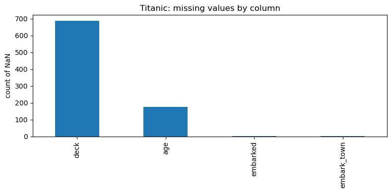
Figure1: Imagegeneratedbytheprovidedcode.

Readingthetable/plot: age, embarked,andespecially deck o enhavemissing values.We’llfocusonfeaturesusedinearlierchapters(sex, class, embarked, age, fare)tokeepthepipelineconsistent.

Simpleimputation

(mean/median/most-frequent/constant)

SimpleImputer isastrongbaseline:

• Numeric: median isrobusttooutliers; mean ifdistributionissymmetric.

• Categorical: most_frequent ora constant like "Unknown".

WewillbuildapipelineforTitanicclassiﬁcationwith imputation+encoding+ logisticregression.

1 from sklearn.compose import ColumnTransformer 2 from sklearn.preprocessing import OneHotEncoder

X = titanic[["sex", "class", "embarked", "age", "fare"]]. copy()

y = titanic["survived"].copy()

try:

ohe = OneHotEncoder(handle_unknown="ignore", sparse_output=False)

except TypeError:

ohe = OneHotEncoder(handle_unknown="ignore", sparse_output=False)

pre_simple = ColumnTransformer(

transformers=[

("nominal", Pipeline([

("imp", SimpleImputer(strategy="most_frequent ")),

("ohe", ohe),

]), nominal),

("ordinal", Pipeline([

("imp", SimpleImputer(strategy="most_frequent ")),

#encode 'class' asordinalThird<Second< First

("ord", OneHotEncoder(handle_unknown="ignore" , drop=None, sparse_output=False) # simpleOHEforclass

if hasattr(OneHotEncoder, "sparse_output") 32 else OneHotEncoder(handle_unknown="ignore", drop=None, sparse_output=False)),

]), ordinal),

("numeric", Pipeline([

("imp", SimpleImputer(strategy="median")),

]), numeric),

)

pipe_simple = Pipeline([

("prep", pre_simple),

("clf", LogisticRegression(max_iter=1000))

scores = cross_val_score(pipe_simple, X, y, cv=5, scoring ="accuracy", n_jobs=-1)

print("Accuracywithsimpleimputation:", scores.mean(). round(3)) 1 from sklearn.compose import ColumnTransformer

from sklearn.preprocessing import OneHotEncoder

from sklearn.impute import SimpleImputer

from sklearn.pipeline import Pipeline

from sklearn.linear_model import LogisticRegression

from sklearn.model_selection import cross_val_score

X = titanic[["sex", "class", "embarked", "age", "fare"]]. copy()

= OneHotEncoder(handle_unknown="ignore", sparse_output=False)

except TypeError:

= OneHotEncoder(handle_unknown="ignore", sparse_output=False)

transformers=[

23 ("nominal", Pipeline([

("imp", SimpleImputer(strategy="most_frequent ")),

("ohe", ohe),

]), nominal),

27 ("ordinal", Pipeline([ 28 ("imp", SimpleImputer(strategy="most_frequent ")),

29 #encode 'class' asordinalThird<Second< First

30 ("ord", OneHotEncoder(handle_unknown="ignore" , drop=None, sparse_output=False) # simpleOHEforclass 31 if hasattr(OneHotEncoder, "sparse_output") 32 else OneHotEncoder(handle_unknown="ignore", drop=None, sparse_output=False)), 33 ]), ordinal), 34 ("numeric", Pipeline([

("imp", SimpleImputer(strategy="median")),

]), numeric),

], 38 verbose_feature_names_out=False

)

41 pipe_simple = Pipeline([ 42 ("prep", pre_simple), 43 ("clf", LogisticRegression(max_iter=1000))

])

scores = cross_val_score(pipe_simple, X, y, cv=5, scoring ="accuracy", n_jobs=-1)

47 print("Accuracywithsimpleimputation:", scores.mean(). round(3))

1 Accuracywithsimpleimputation:0.789

Addingmissingnessindicators

Sometimes whetheravalueismissingispredictive (e.g.,peoplewithout recorded age di ersystematically).

Wecanappendindicatorcolumns.Thesimplestpathis SimpleImputer( add_indicator=True) (ifsupported)or MissingIndicator. We’llattempt add_indicator=True andfallbackto MissingIndicator if needed.

pre_with_ind = ColumnTransformer(

transformers=[

("nominal", nominal_block_with_indicator(), nominal),

("ordinal", Pipeline([

("imp", SimpleImputer(strategy="most_frequent ")),

("ohe", ohe),

]), ordinal),

("numeric", numeric_block_with_indicator(), numeric),

verbose_feature_names_out=False

pipe_with_ind = Pipeline([

("prep", pre_with_ind),

("clf", LogisticRegression(max_iter=1000))

scores_ind = cross_val_score(pipe_with_ind, X, y, cv=5, scoring="accuracy", n_jobs=-1)

print("Accuracywithindicators:", scores_ind.mean(). round(3))

("imp", SimpleImputer(strategy="most_frequent " , add_indicator=True)),

("ohe", ohe),

except TypeError:

return Pipeline([

("imp", SimpleImputer(strategy="most_frequent ")),

("ohe", ohe),

def numeric_block_with_indicator():

try:

return Pipeline([

("imp", SimpleImputer(strategy="median", add_indicator=True)),

])

except TypeError:

return Pipeline([

("imp", SimpleImputer(strategy="median")),

])

pre_with_ind = ColumnTransformer(

transformers=[

("nominal", nominal_block_with_indicator(), nominal),

("ordinal", Pipeline([

("imp", SimpleImputer(strategy="most_frequent ")),

("ohe", ohe),

]), ordinal),

("numeric", numeric_block_with_indicator(), numeric),

verbose_feature_names_out=False

)

39 pipe_with_ind = Pipeline([

("prep", pre_with_ind),

("clf", LogisticRegression(max_iter=1000))

])

scores_ind = cross_val_score(pipe_with_ind, X, y, cv=5, scoring="accuracy", n_jobs=-1) 45 print("Accuracywithindicators:", scores_ind.mean(). round(3))

1 Accuracywithindicators:0.799

Interpretingtheresult: Ifaccuracyimproves,themodelisbeneﬁtingfromthe informationcontainedinthepatternofmissingness.

KNNImputer(neighbors-basedimputation)

KNNImputer imputesavaluefrom similarrows (nearestneighbors).

Pros:usesmultivariatestructure.Cons:slower,sensitivetoscaleandsparsecategories.

Wewill:

• One-hotencodecategoricalsﬁrst(sodistanceismeaningful),

• Scalenumericcolumns(optionalbutrecommended),

• ThenapplyKNNImputeronthe combined featurespace.

1 from sklearn.impute import KNNImputer 2 from sklearn.preprocessing import StandardScaler

4 pre_knn = ColumnTransformer( 5 transformers=[ 6 ("nominal", Pipeline([ 7 ("imp", SimpleImputer(strategy="most_frequent ")), 8 ("ohe", ohe),

]), nominal),

("ordinal", Pipeline([

("imp", SimpleImputer(strategy="most_frequent ")),

("ohe", ohe),

]), ordinal),

("numeric", Pipeline([

("imp", SimpleImputer(strategy="median")), 16 ("sc", StandardScaler()), 17 ]), numeric),

verbose_feature_names_out=False

22 pipe_knn = Pipeline([

("prep", pre_knn),

("knnimp", KNNImputer(n_neighbors=5, weights=" distance")),

("clf", LogisticRegression(max_iter=1000))

])

28 scores_knn = cross_val_score(pipe_knn, X, y, cv=5, scoring="accuracy", n_jobs=-1)

print("AccuracywithKNNImputer:", scores_knn.mean(). round(3))

1 from sklearn.impute import KNNImputer 2 from sklearn.preprocessing import StandardScaler

4 pre_knn = ColumnTransformer(

transformers=[

("nominal", Pipeline([

("imp", SimpleImputer(strategy="most_frequent ")), 8 ("ohe", ohe),

]), nominal),

("ordinal", Pipeline([

("imp", SimpleImputer(strategy="most_frequent ")),

("ohe", ohe),

]), ordinal),

("numeric", Pipeline([

("imp", SimpleImputer(strategy="median")),

("sc", StandardScaler()),

]), numeric),

verbose_feature_names_out=False

pipe_knn = Pipeline([ 23 ("prep", pre_knn),

24 ("knnimp", KNNImputer(n_neighbors=5, weights=" distance")),

25 ("clf", LogisticRegression(max_iter=1000))

26 ])

28 scores_knn = cross_val_score(pipe_knn, X, y, cv=5, scoring="accuracy", n_jobs=-1)

29 print("AccuracywithKNNImputer:", scores_knn.mean(). round(3))

1 AccuracywithKNNImputer:0.789

Notes:

• KNNImputeroccurs a er encoding/scalingsodistancesreﬂectallfeatures.

• Tune n_neighbors; weights="distance" canhelpwhenneighbors varyinsimilarity.

IterativeImputer(multivariate,model-based)

IterativeImputer modelseachfeaturewithmissingvaluesasafunctionofother features(round-robin).

Pros:powerfulwhenrelationshipsareapproximatelylinear/non-lineardepending onestimator.

Cons:heavier,morehyperparameters.

We’llusealinearestimator(defaultBayesianRidge)forspeedandstability.

1 #EnableIterativeImputerifneededinolderversions 2 try:

3 from sklearn.impute import IterativeImputer 4 except Exception: 5 from sklearn.experimental import enable_iterative_imputer #noqa:F401 6 from sklearn.impute import IterativeImputer

8 pre_iter = pre_knn #reuseencoding/scalingblockfrom

("prep", pre_iter),

("iterimp", IterativeImputer(max_iter=10, random_state=42, sample_posterior=False)),

("clf", LogisticRegression(max_iter=1000))

print("AccuracywithIterativeImputer:", scores_iter.mean ().round(3)) 1 #EnableIterativeImputerifneededinolderversions

try: 3 from sklearn.impute import IterativeImputer

except Exception: 5 from sklearn.experimental import enable_iterative_imputer #noqa:F401

from sklearn.impute import IterativeImputer

("prep", pre_iter),

("iterimp", IterativeImputer(max_iter=10, random_state=42, sample_posterior=False)),

("clf", LogisticRegression(max_iter=1000))

= cross_val_score(pipe_iter, X, y, cv=5, scoring="accuracy", n_jobs=-1)

print("AccuracywithIterativeImputer:", scores_iter.mean ().round(3)) 1 AccuracywithIterativeImputer:0.789

Visualcheck:distributionbefore/a

Wewillcomparethe age distributionbeforeimputationvsa ersimplemedian imputation.

Thishelpsverifythatimputationdidnotcreateunrealisticspikesordistortions.

1 #Extract 'age' beforeandafterasimplemedian imputationforplotting

2 age_raw = X["age"]

4 median_imp = SimpleImputer(strategy="median")

5 age_imp = pd.Series(median_imp.fit_transform(X[["age"]]). ravel(), name="age_imputed")

7 plt.figure(figsize=(8,4))

8 plt.hist(age_raw.dropna(), bins=20, alpha=0.6, label="age (raw)")

9 plt.hist(age_imp, bins=20, alpha=0.6, label="age(medianimputed)")

10 plt.legend()

11 plt.title("Agedistribution:rawvsmedian-imputed")

12 plt.tight_layout()

13 plt.show()

1 #Extract 'age' beforeandafterasimplemedian imputationforplotting

2 age_raw = X["age"]

4 median_imp = SimpleImputer(strategy="median")

5 age_imp = pd.Series(median_imp.fit_transform(X[["age"]]). ravel(), name="age_imputed")

7 plt.figure(figsize=(8,4))

8 plt.hist(age_raw.dropna(), bins=20, alpha=0.6, label="age (raw)")

9 plt.hist(age_imp, bins=20, alpha=0.6, label="age(medianimputed)")

10 plt.legend()

11 plt.title("Agedistribution:rawvsmedian-imputed")

12 plt.tight_layout()

13 plt.show()

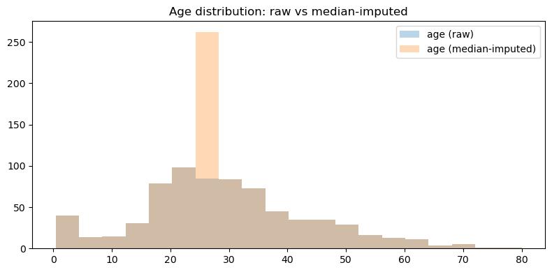
Figure2: Imagegeneratedbytheprovidedcode.

Readingtheplot: Medianimputationﬁllsgapswithoutchangingthecentraltendency,butcan inﬂate themedianbin.Advancedimputers(KNN/Iterative)can preserveshapebetter—validatewithmetrics.

Leakage-safeevaluation:quickcomparison

Let’ssummarizethe CVaccuracy forthedi erentstrategieswetried. Becauseeachimputerlives inside thepipeline,thereis noleakage fromvalidation folds.

1 import pandasaspd

3 acc_table = pd.DataFrame({

4 "SimpleImputer":[scores.mean() for scores in [scores ]][0],

5 "WithIndicators":[scores_ind.mean() for scores_ind in [scores_ind]][0],

6 "KNNImputer":[scores_knn.mean() for scores_knn in [ scores_knn]][0],

7 "IterativeImputer":[scores_iter.mean() for scores_iter in [scores_iter]][0],

8 }, index=["CVAccuracy"]).T.sort_values(by="CVAccuracy", ascending=False)

9 10 display(acc_table.round(3))

1 import pandasaspd

3 acc_table = pd.DataFrame({

4 "SimpleImputer":[scores.mean() for scores in [scores ]][0],

5 "WithIndicators":[scores_ind.mean() for scores_ind in [scores_ind]][0],

6 "KNNImputer":[scores_knn.mean() for scores_knn in [ scores_knn]][0],

7 "IterativeImputer":[scores_iter.mean() for scores_iter in [scores_iter]][0],

8 }, index=["CVAccuracy"]).T.sort_values(by="CVAccuracy", ascending=False)

9 10 display(acc_table.round(3))

0.789

IterativeImputer

0.789 Summary

• Startwith SimpleImputer (medianfornumeric,most-frequentforcategorical).It’srobustandfast.

• Ifperformancesu ersandyoususpectstructureinmissingness,try missingnessindicators.

• Consider KNNImputer or IterativeImputer whenvariableshavestrongrelationshipsandsimplestrategiesunderperform.

• Keepimputers insidepipelines toavoidleakage.Tuneimputerhyperparameterswithcross-validationasyouwouldanymodel.

• For MNAR,modelingmissingnessexplicitly(two-stagemodels,selection models)orcollectingmoredatamaybenecessary.