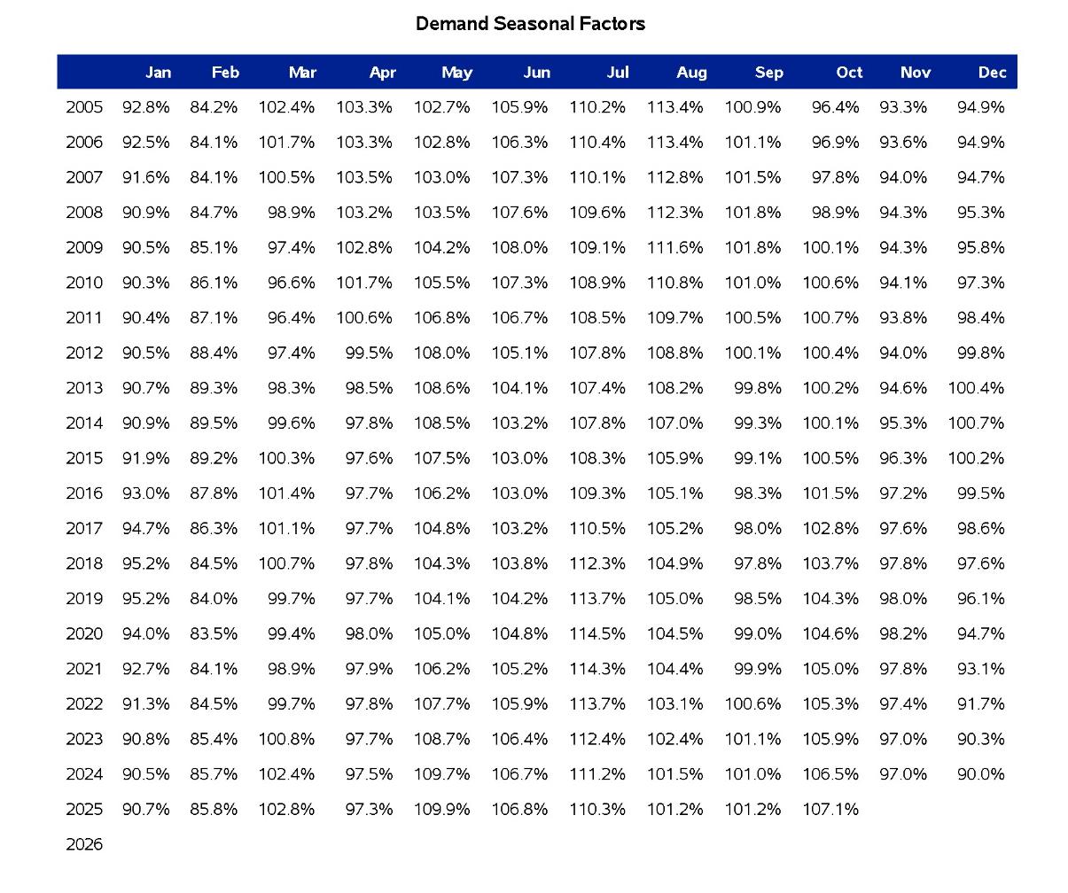
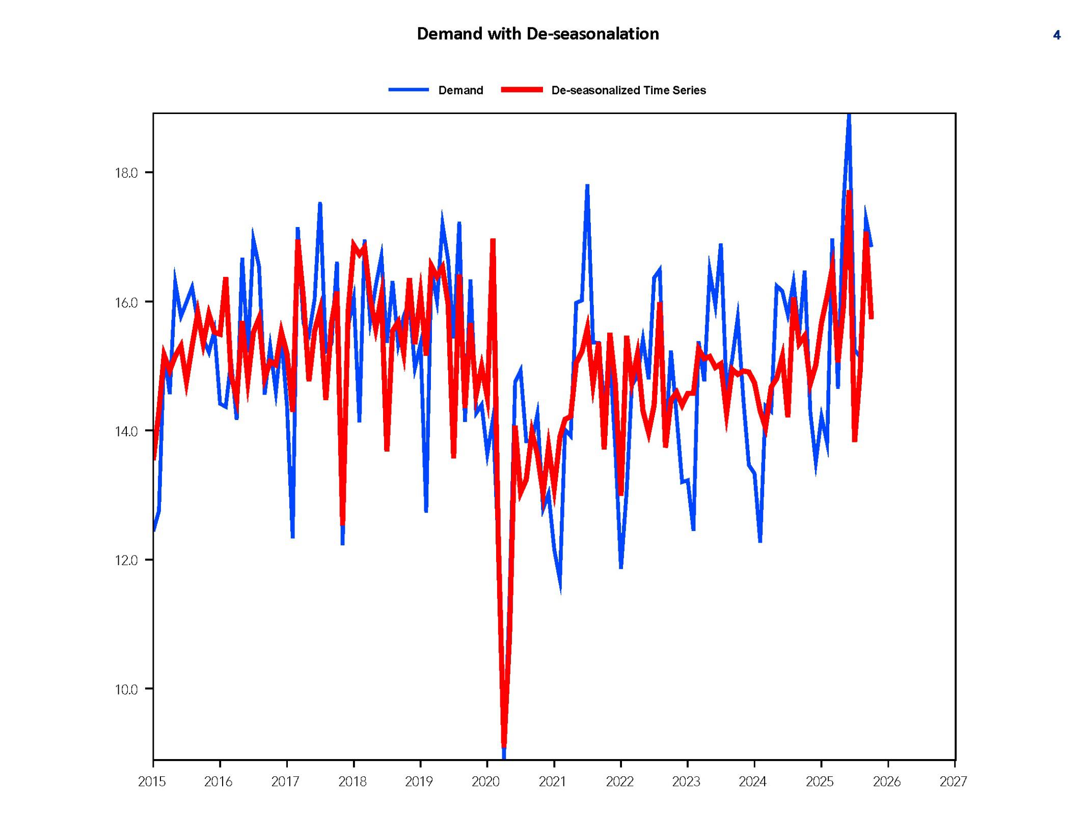
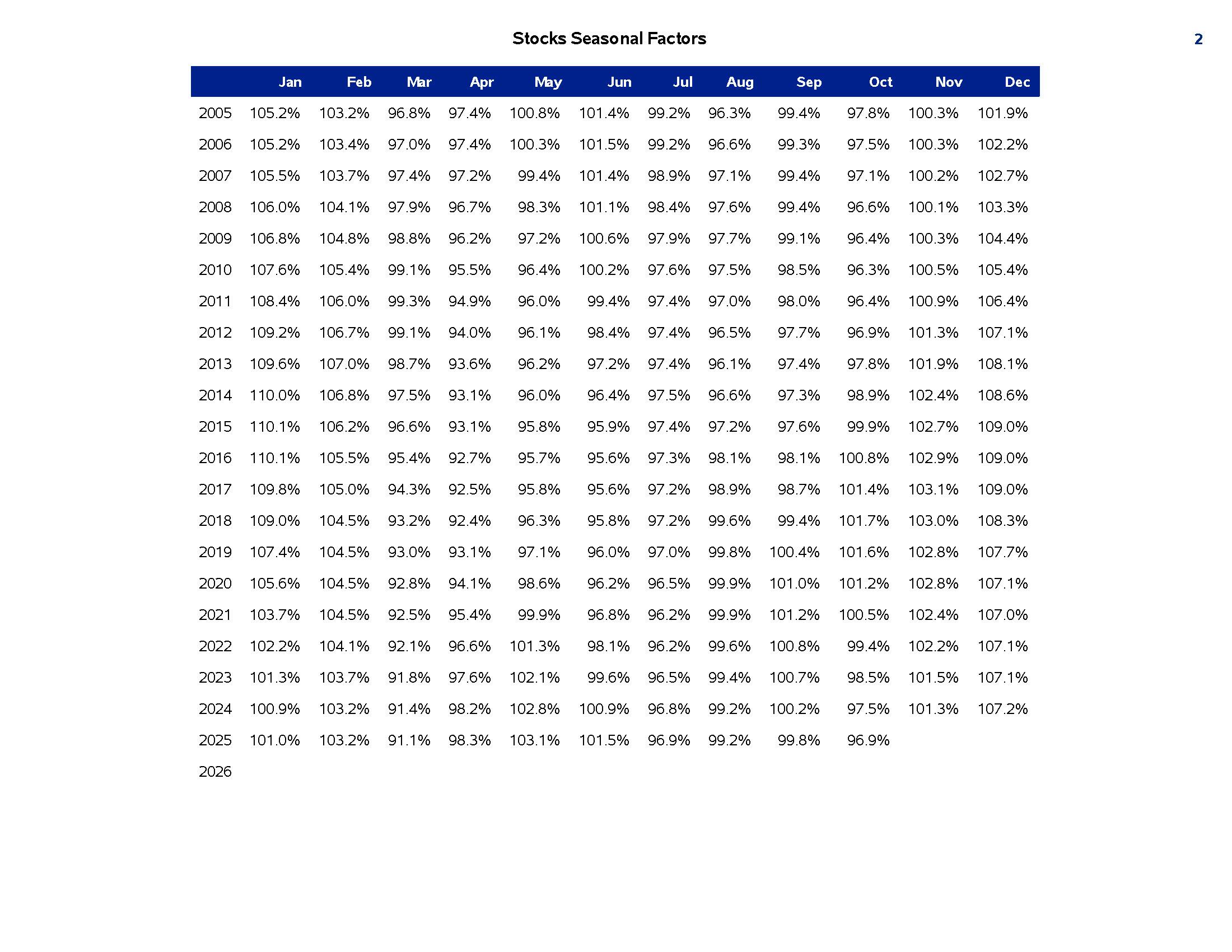
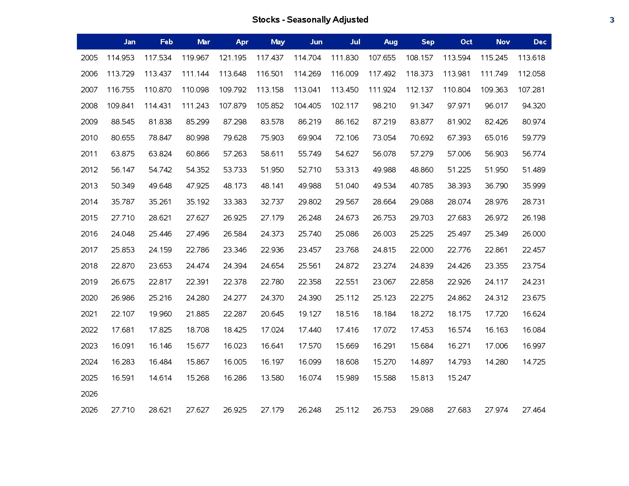
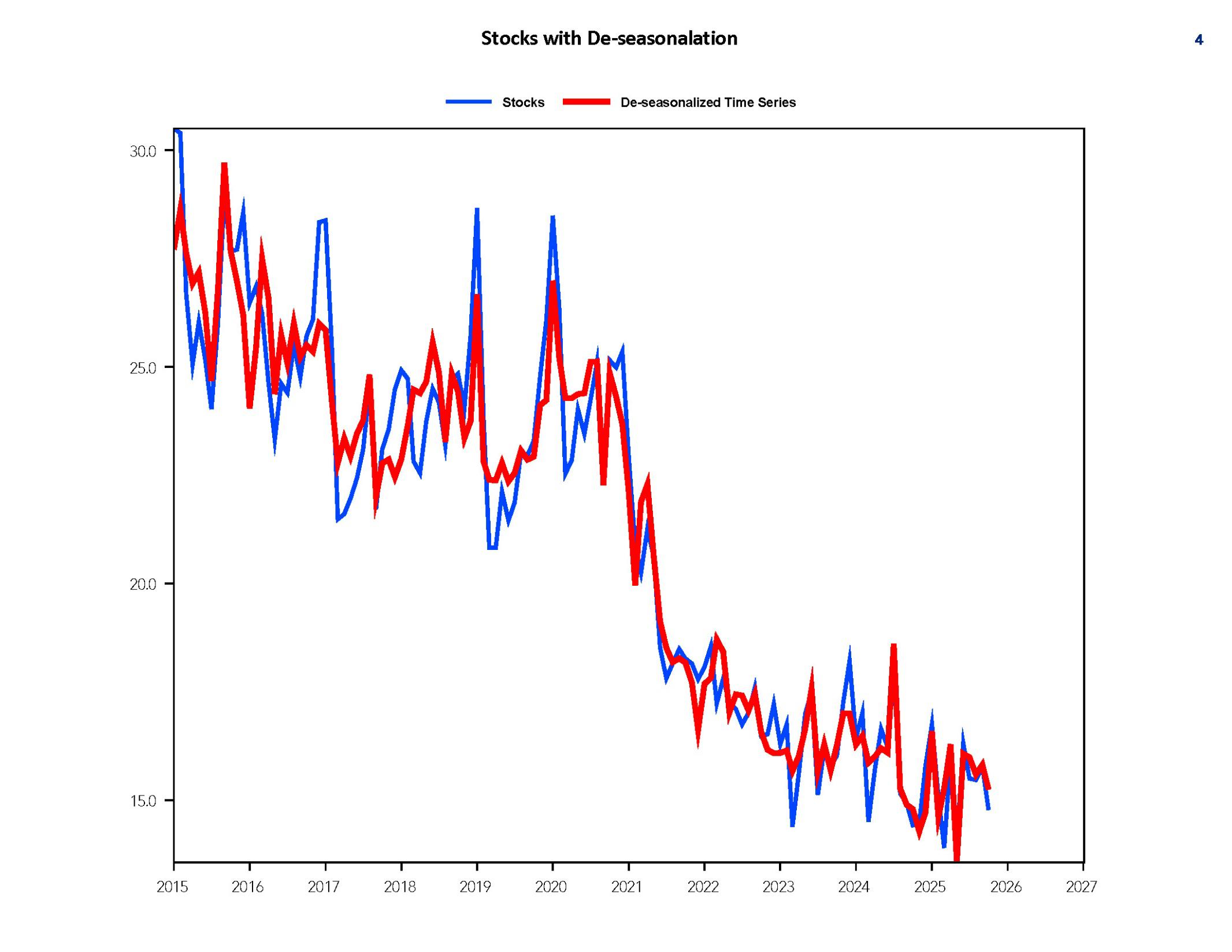
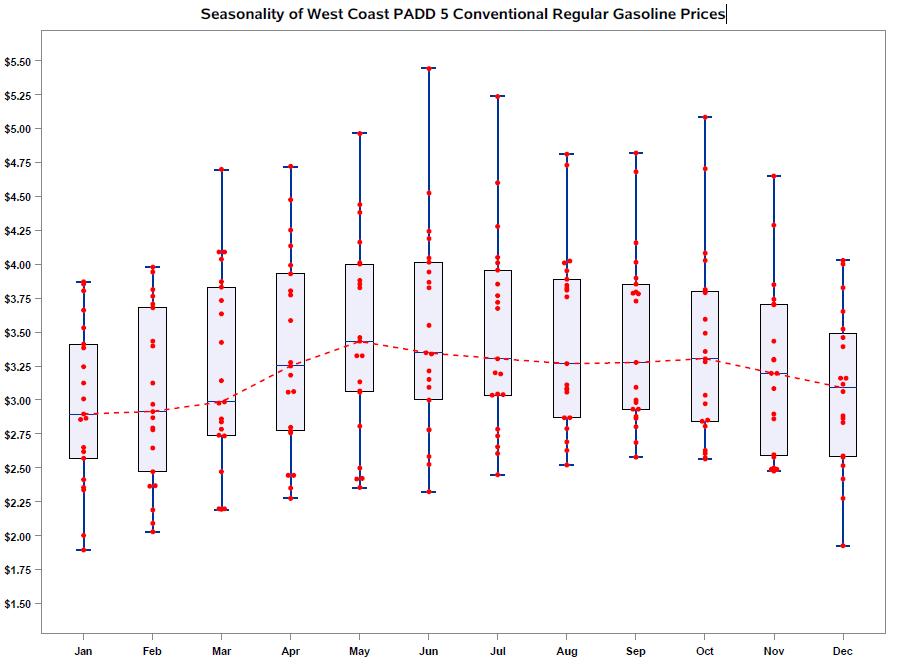
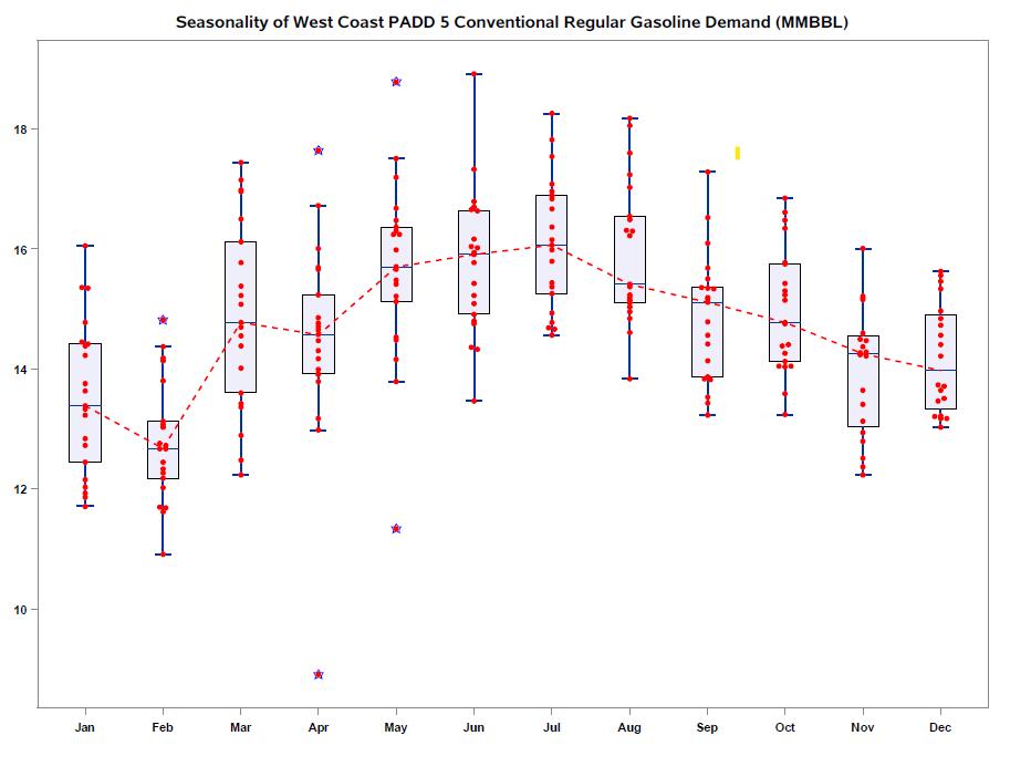
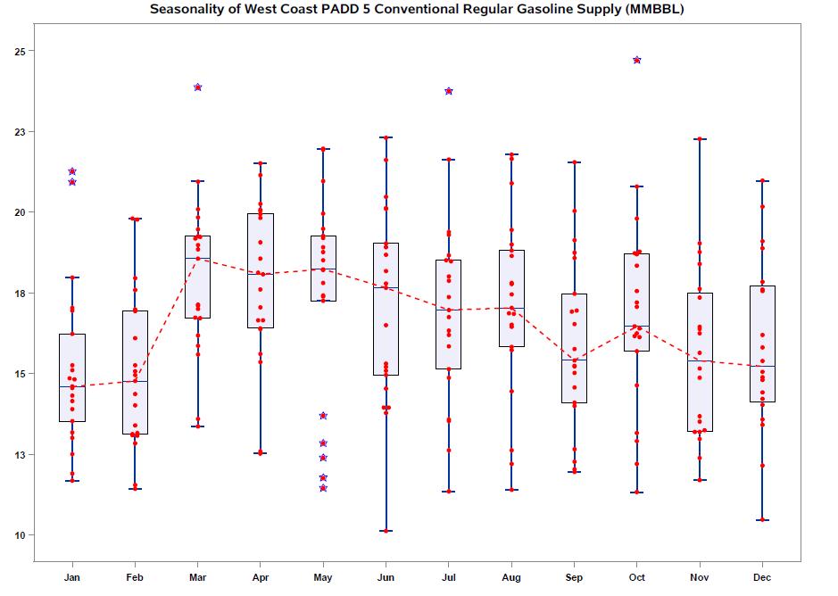
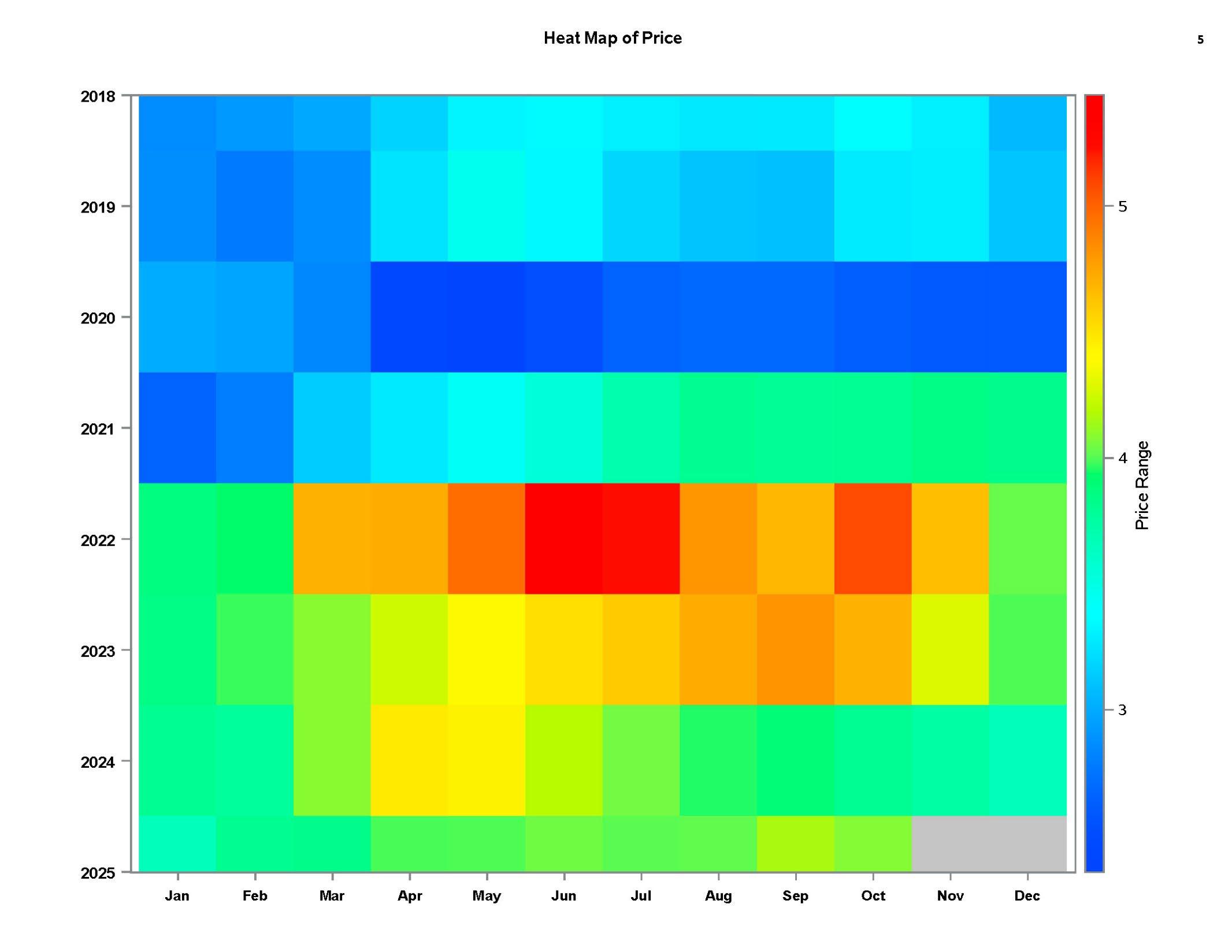
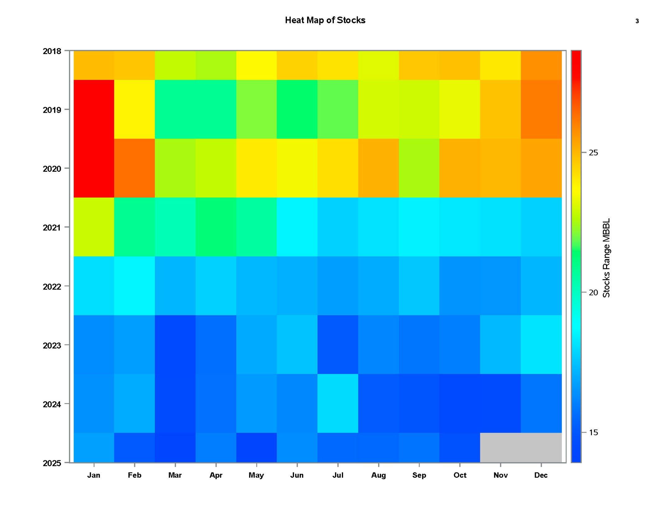
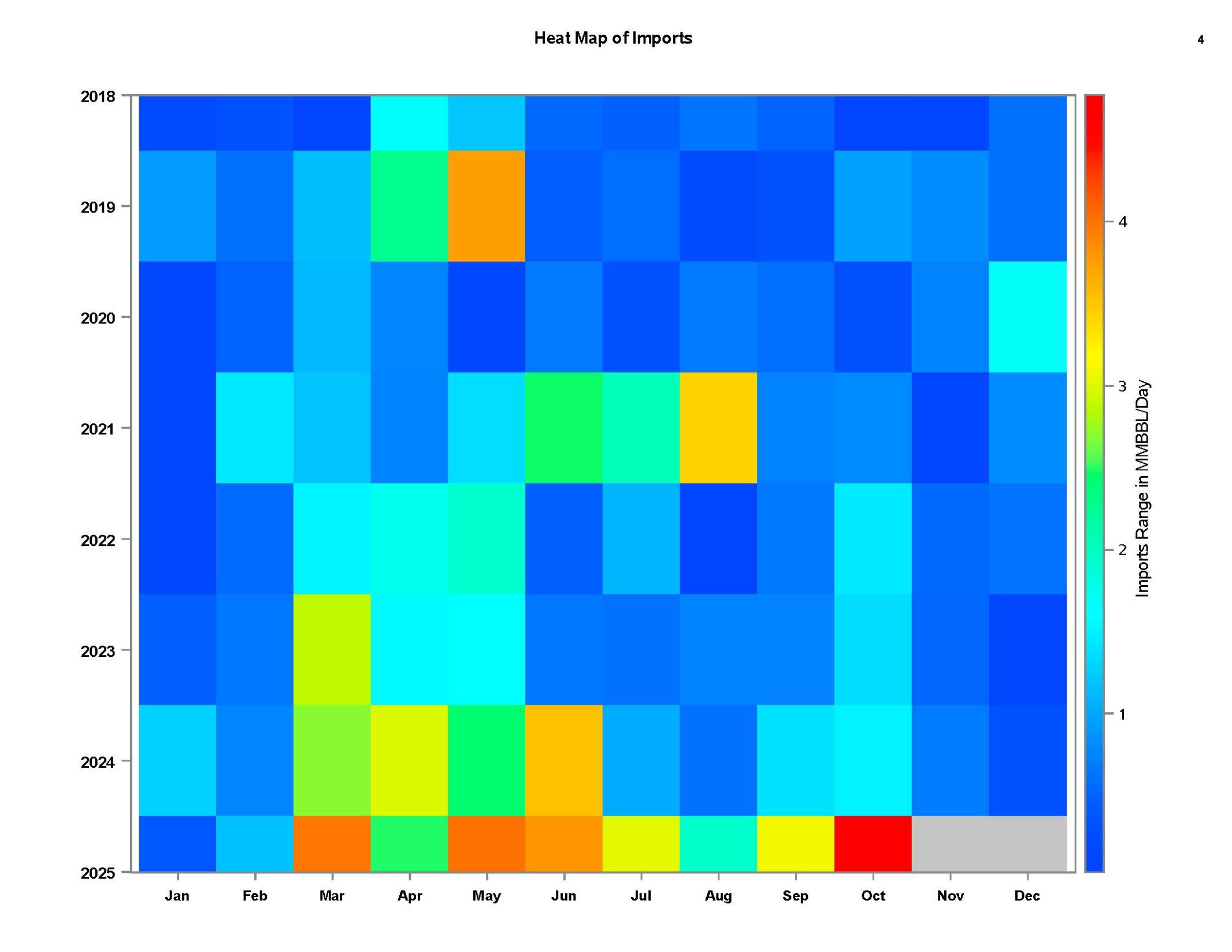
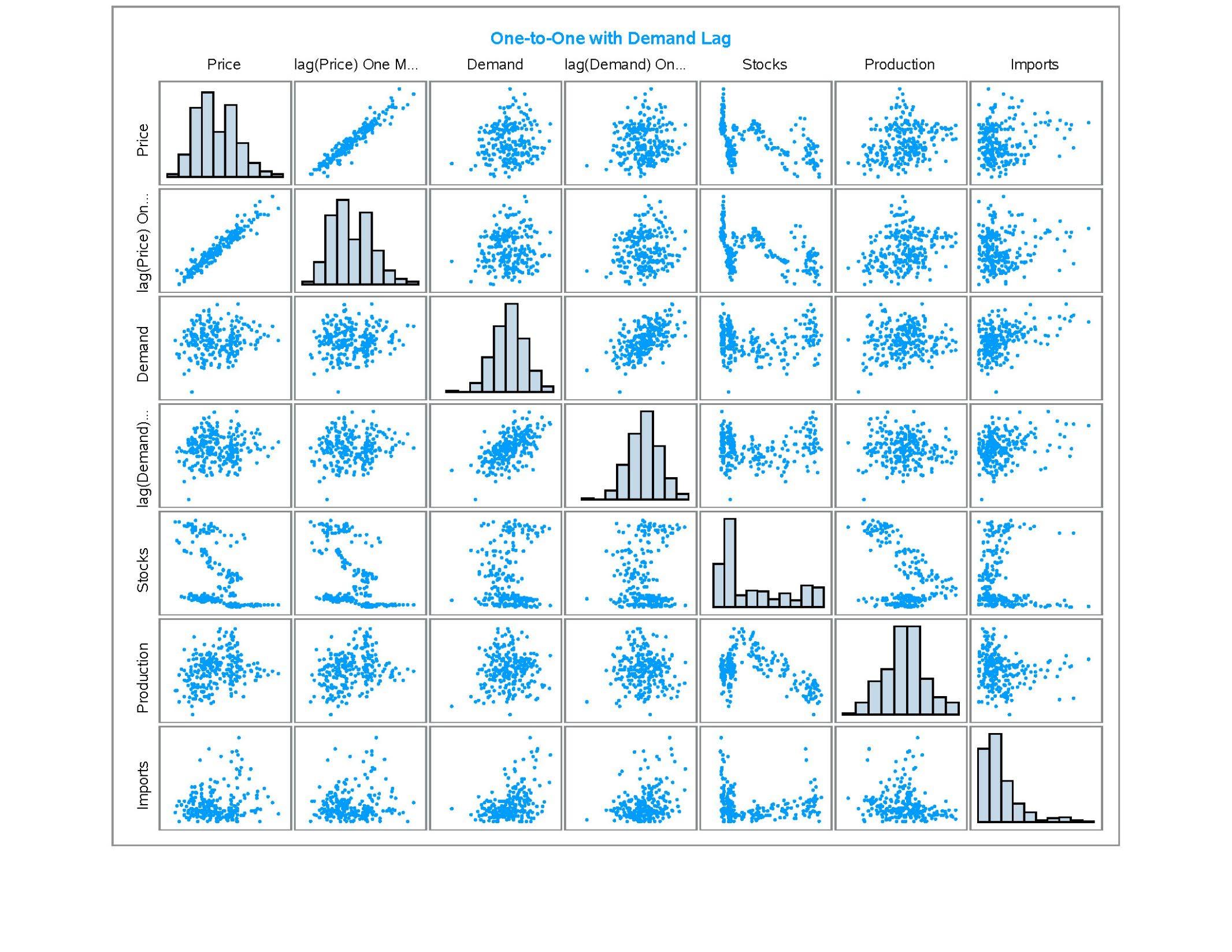
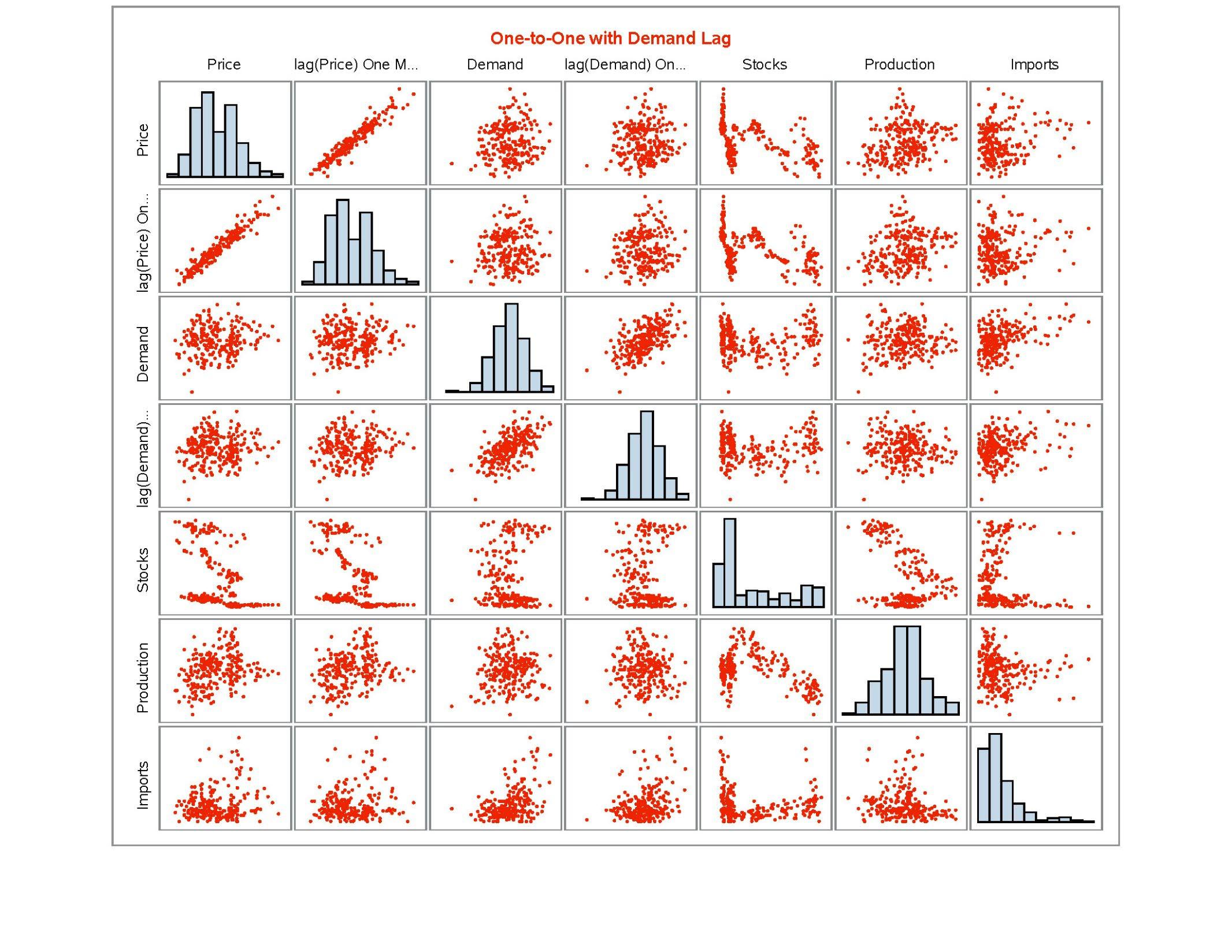
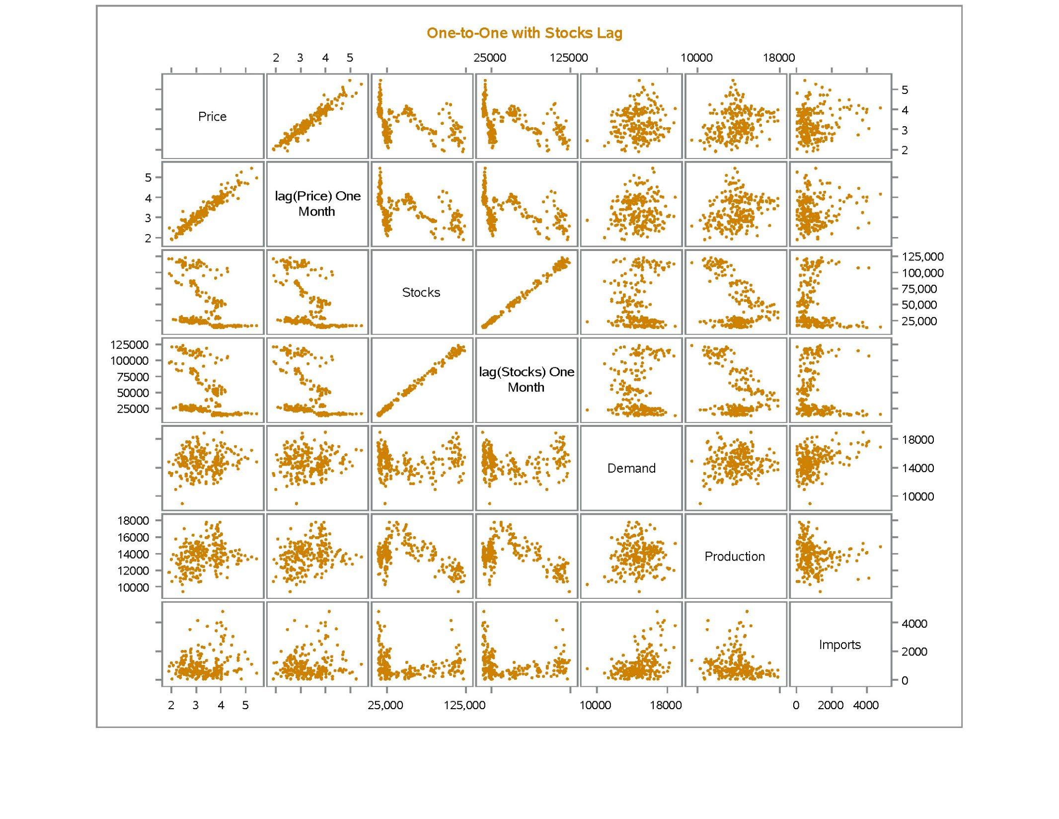
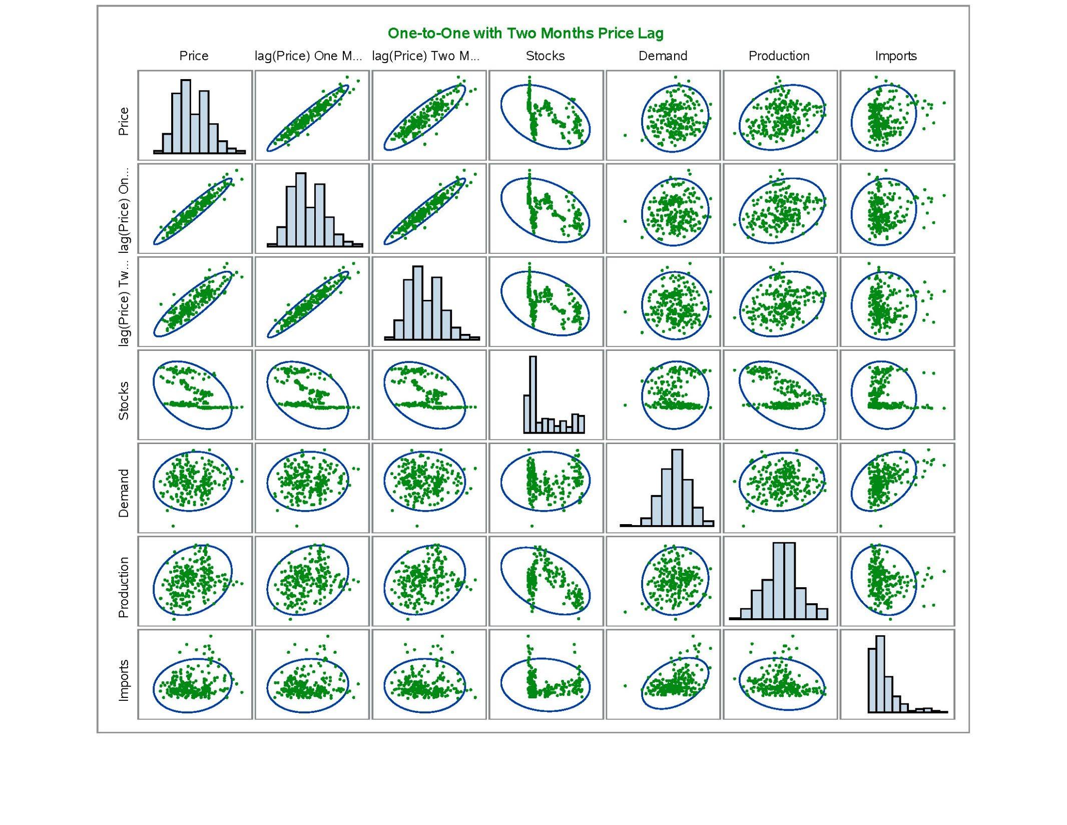
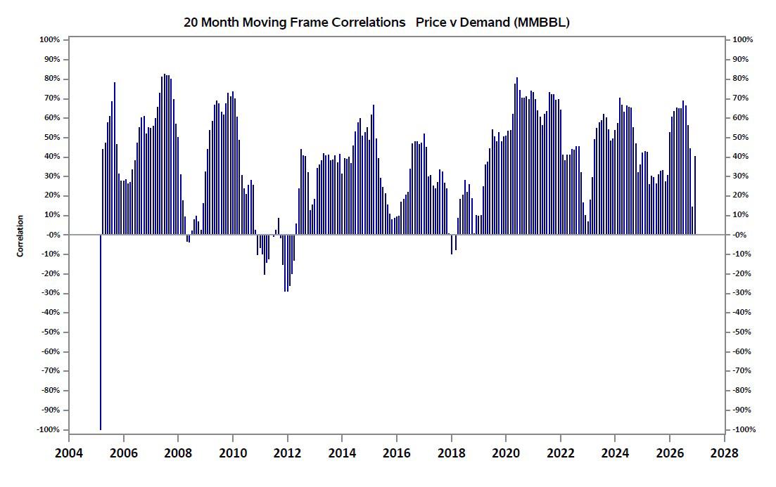
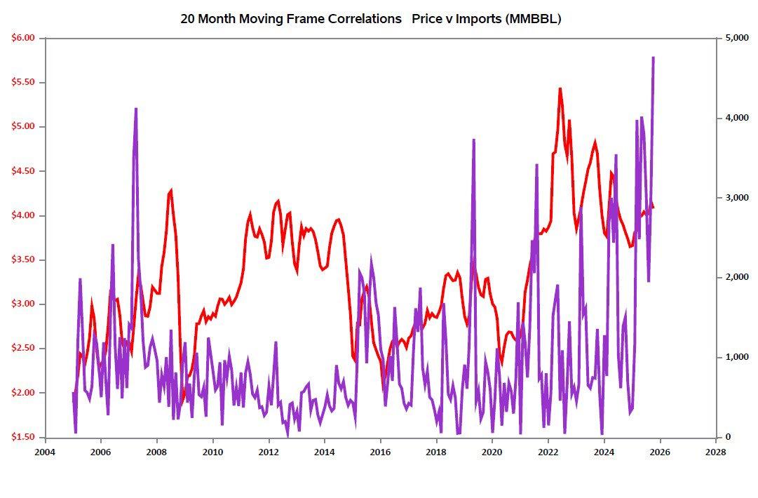
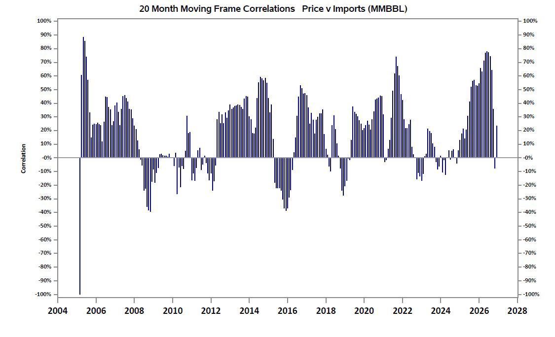
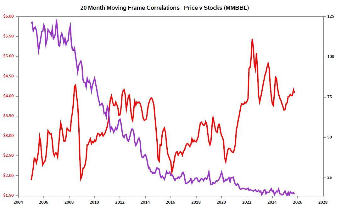
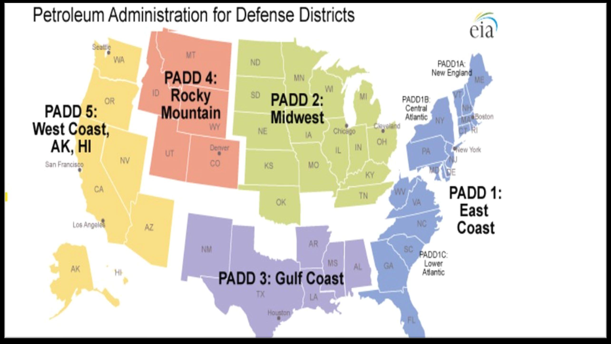
Using statistics and modeling this report will show numerically that in the West Coast (PADD 5) Conventional Gasoline Market
Demand Persistence Dominate
Short-run gasoline demand is highly persistent
Prior-period consumption explains most current consumption; short-run price elasticity is small.
Price spikes do NOT immediately suppress gasoline demand
Retail Prices Are Highly Sticky
Retail gasoline prices exhibit strong lag dependence and gradual pass-through
Once prices rise, they tend to remain elevated until physical supply improves
Inventories Are the Primary Shock Absorber
Inventory variation absorbs supply and demand shocks before prices move materially. Monitor inventory draw downs as the leading indicator of price pressure.
The West Coast gasoline market is a high-persistence, inventory-buffered, price-propagating market.
Data Construction and Market Coverage Data Sources Data Management and Retrieval
The analysis begins with the construction of a comprehensive dataset designed to re�lect the physical and economic structure of the PADD 5 gasoline market. The Energy Information Administration (EIA) is the primary source for supply, disposition, and inventory series; California data sources are used where retail or state-level detail is required.
Because the EIA is rich but not always easy to access programmatically, we maintain a curated library of series identi�iers and retrieval code. Series are collected at annual, monthly, and weekly frequencies and aligned to a common calendar so that supply, disposition, and pricing variables can be interpreted coherently.
Data Management and Retrieval
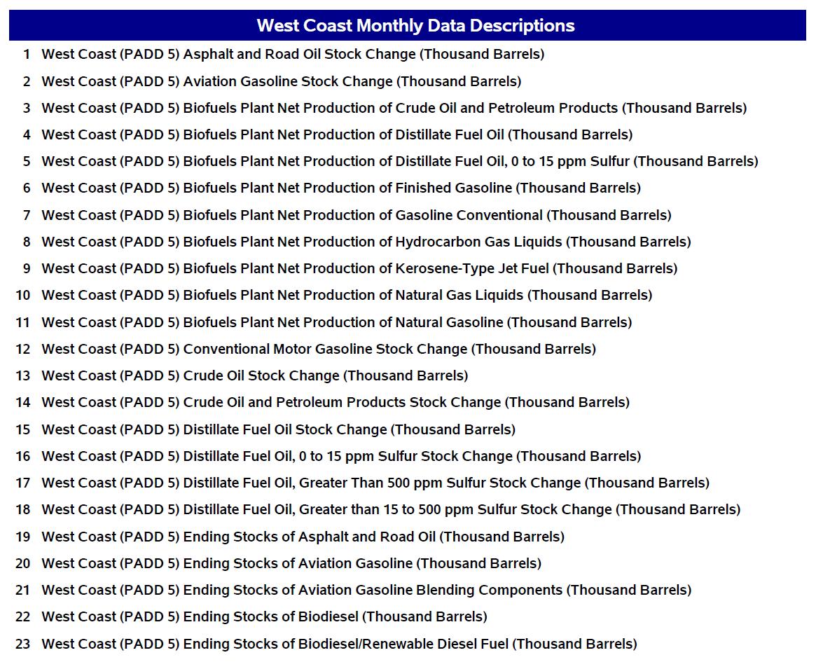
The user simply looks up by alphabetically ordering data that they want to see and by pulling that description and its number the data series can be retrieved very easily. At the time of writing, the data library contains 962 annual series (50 states, DC, and U.S. total), 1,535 monthly PADD series, and 538 weekly PADD series—2,635 time series in total.
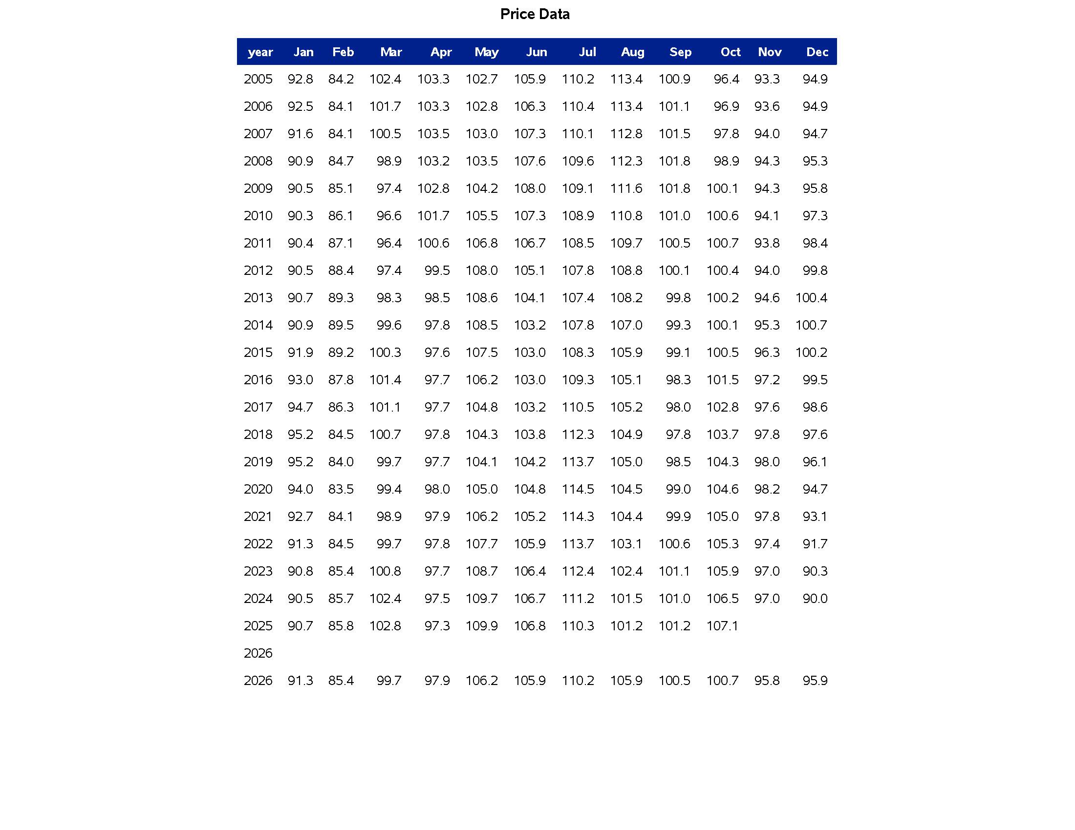
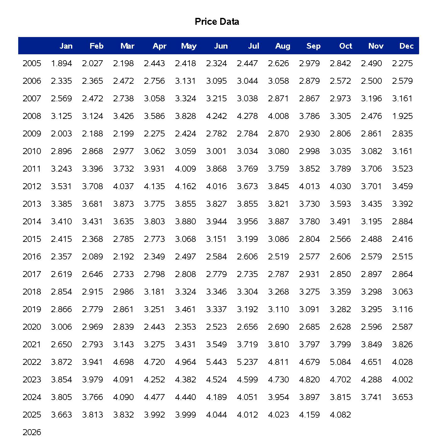
These counts are included to underscore the breadth of market coverage, not to overwhelm the reader. Below is a screenshot from a part of a page of the monthly data
This report is based on the accounting identity.
= Production����
re�ineryoutput + Imports����
imports + NetReceipts����
inter-PADDtransfers + Biofuels
So the following data series were retrieved: (all in Thousand Barrels)
1. Ending Stocks of Conventional Motor Gasoline
2. Re�inery and Blender Net Production of Conventional Motor Gasoline
3. Imports of Conventional Motor Gasoline
4. Net Receipts by Pipeline, Tanker, Barge from Other PADDs of Conventional Motor Gasoline
5. Gasoline Biofuels Plant Net Production of Conventional Motor Gasoline
6. Supply Adjustment of Conventional Motor Gasoline
7. Exports of Conventional Motor Gasoline
8. Product Supplied of Conventional Motor Gasoline
As well as prices
West Coast All Grades Conventional Retail Gasoline Prices (Dollars per Gallon)
West Coast Midgrade Conventional Retail Gasoline Prices (Dollars per Gallon)
West Coast Premium Conventional Retail Gasoline Prices (Dollars per Gallon)
West Coast Regular Conventional Retail Gasoline Prices (Dollars per Gallon)
West Coast Regular Reformulated Retail Gasoline Prices (Dollars per Gallon)
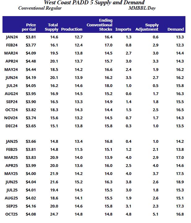
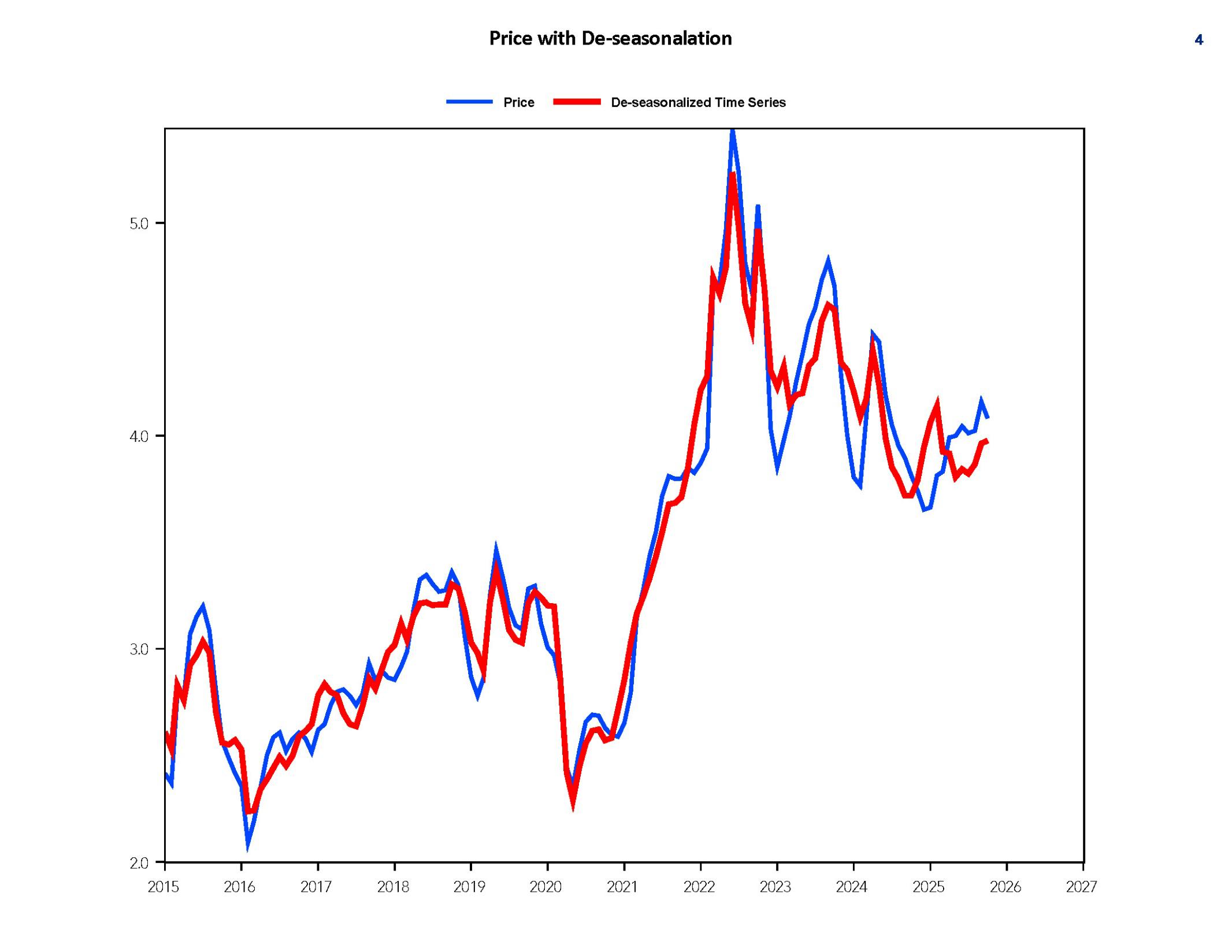
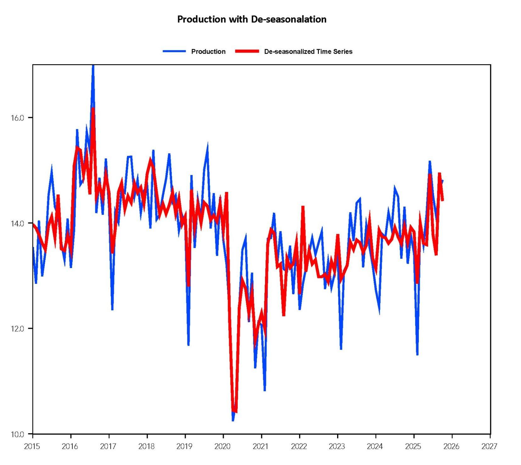
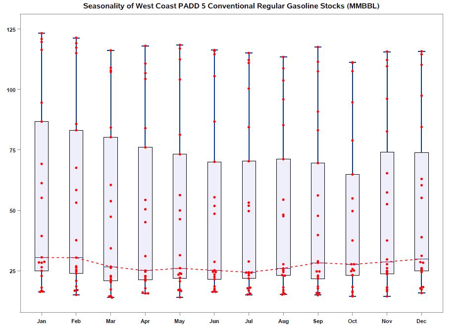
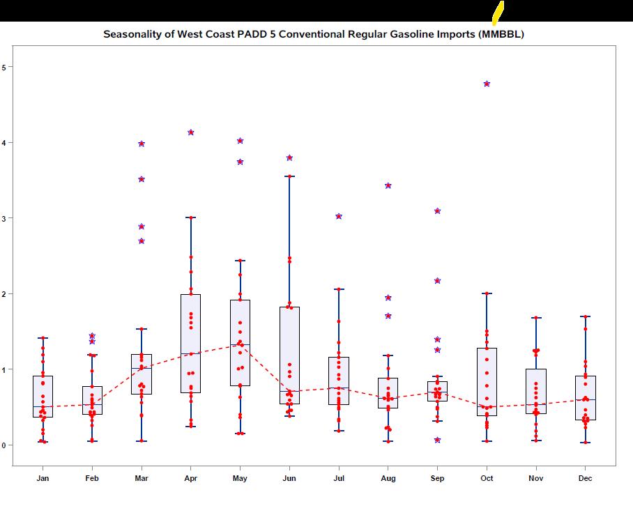
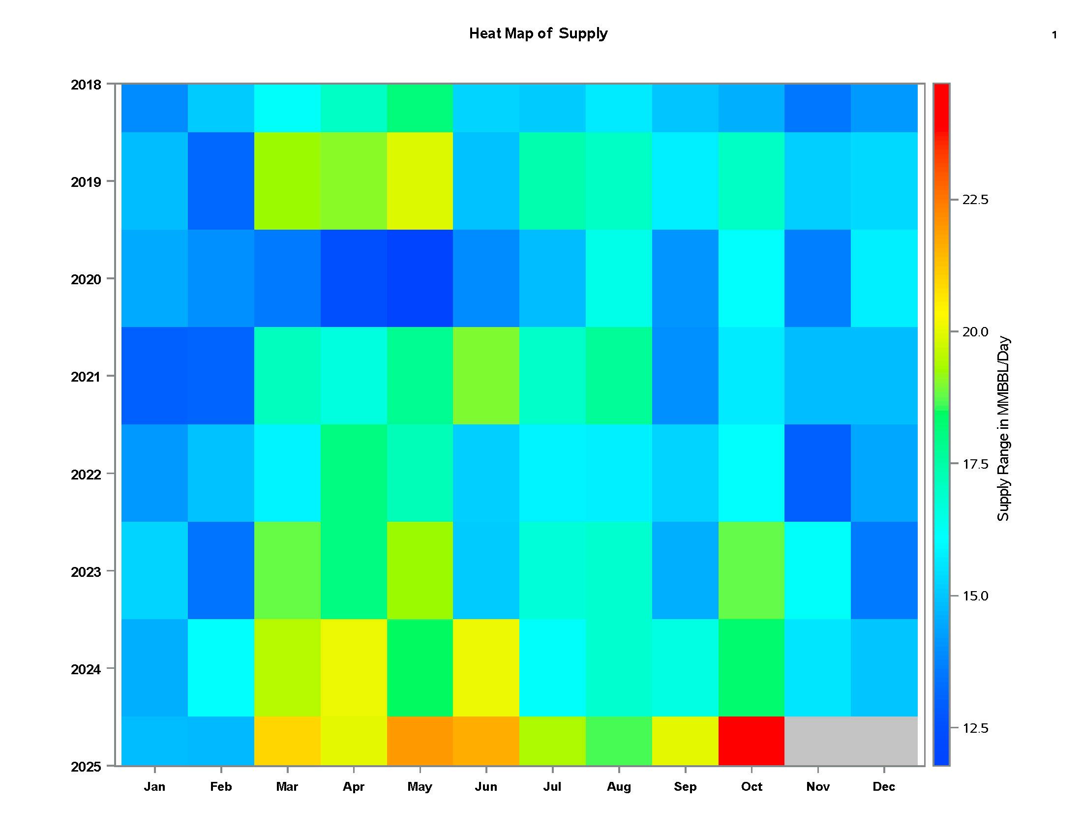
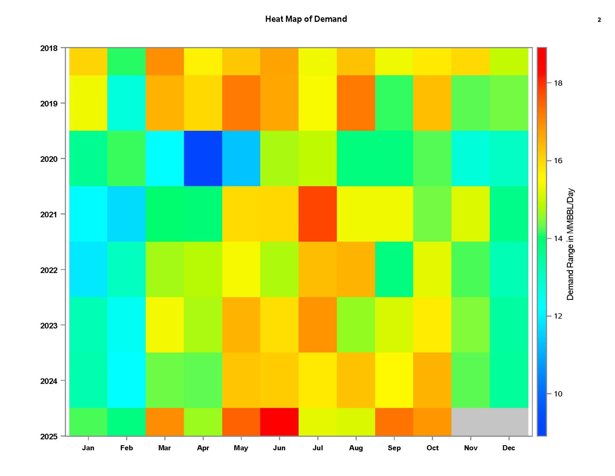
Conventional Regular Gasoline Prices, Production , Demand, Stocks, Import
���� § Time series plots
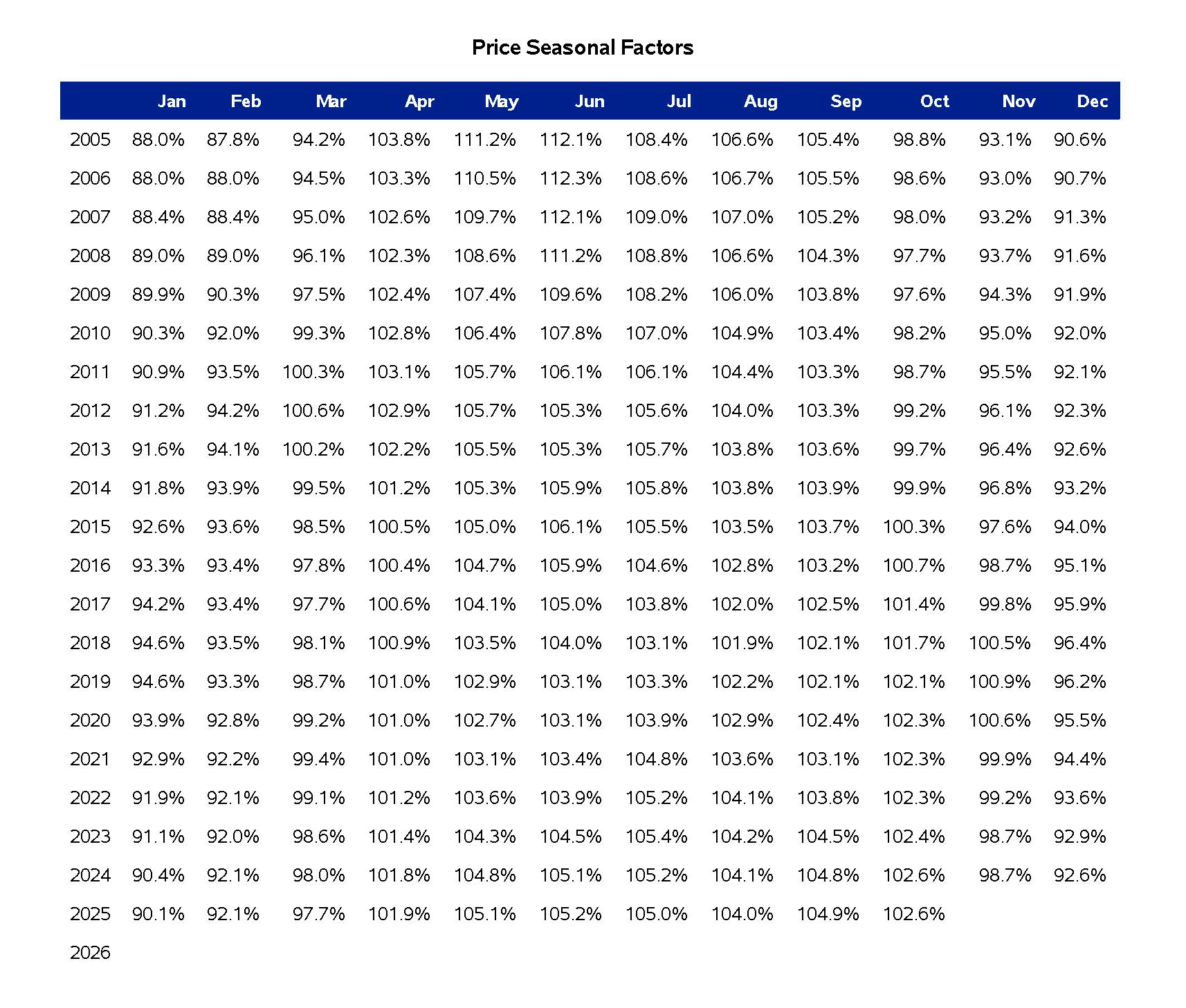
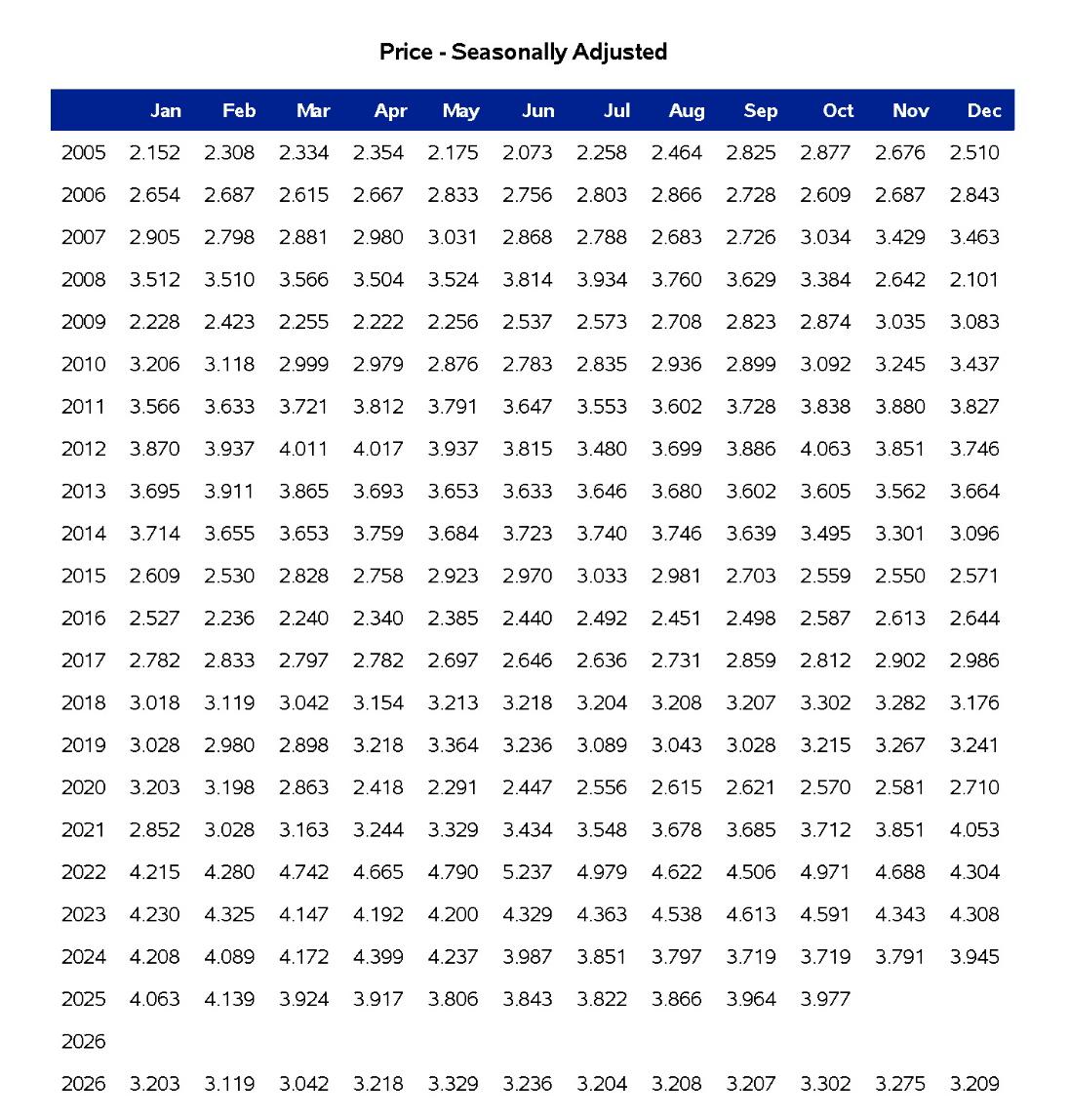
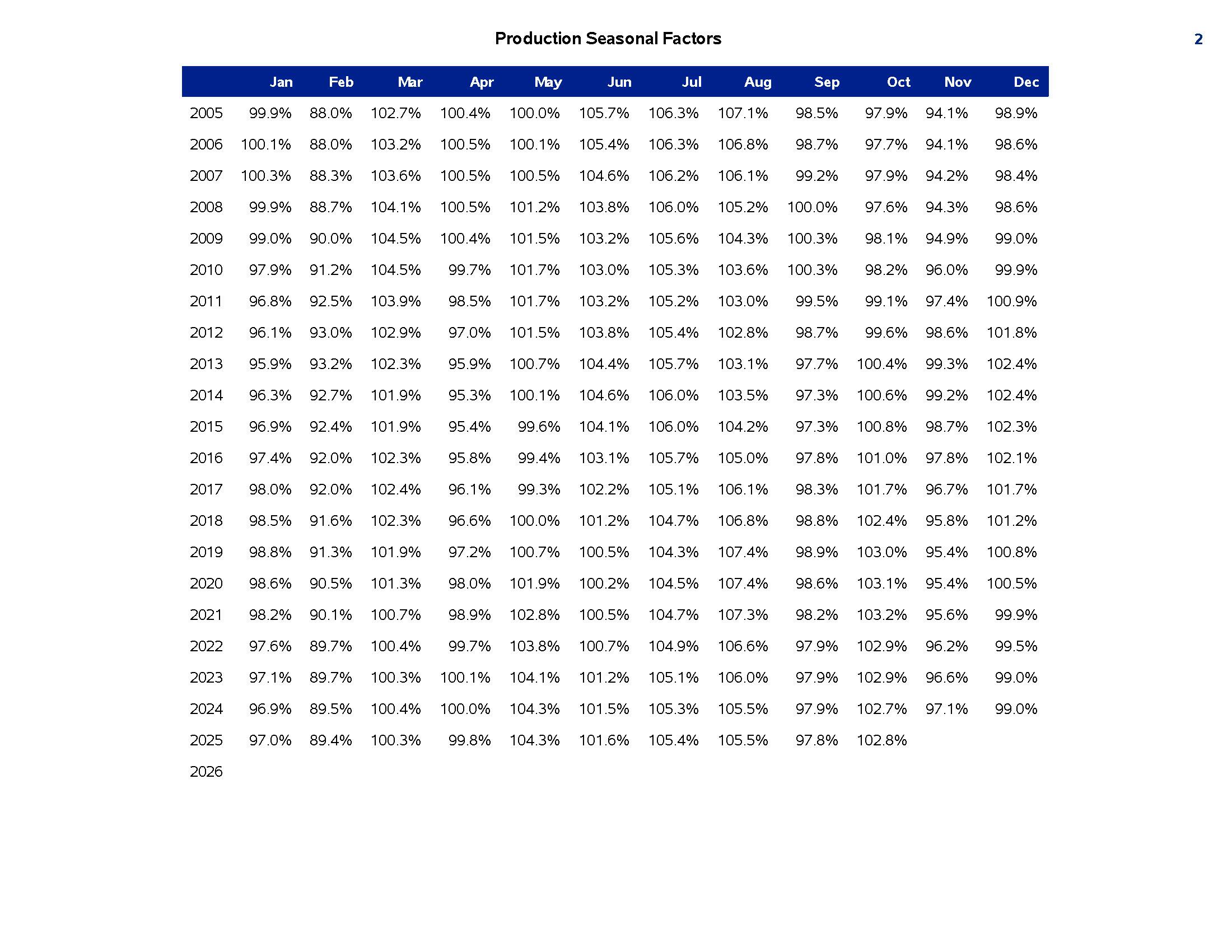
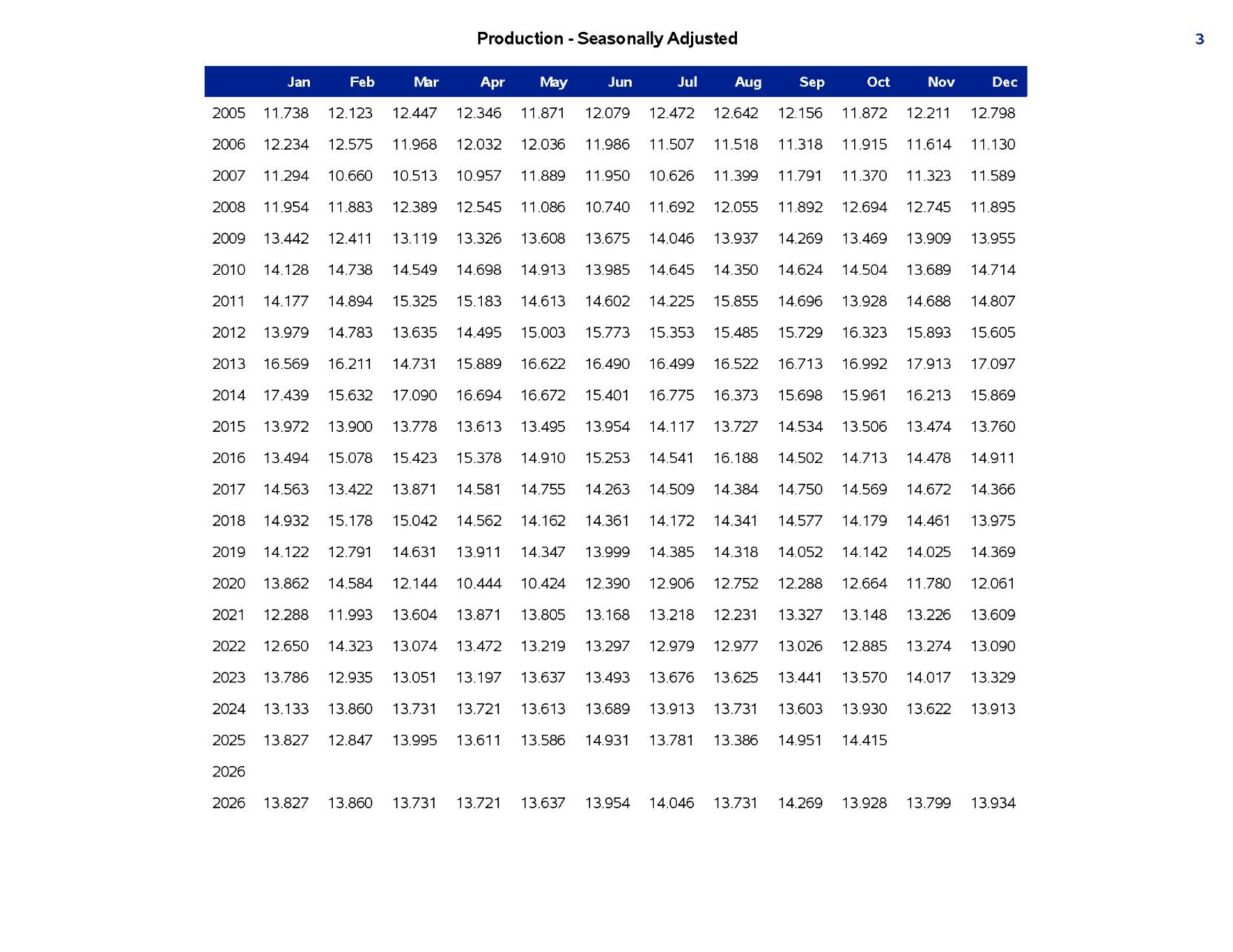
§ X11 tables and plots
§ Distribution plots
§ Heat Maps
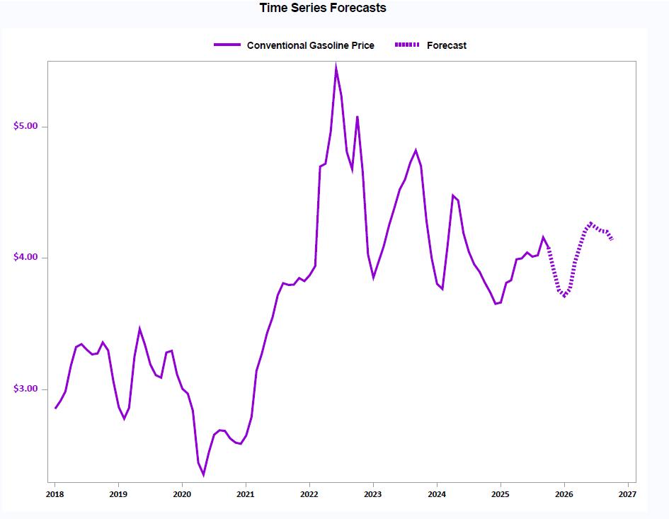
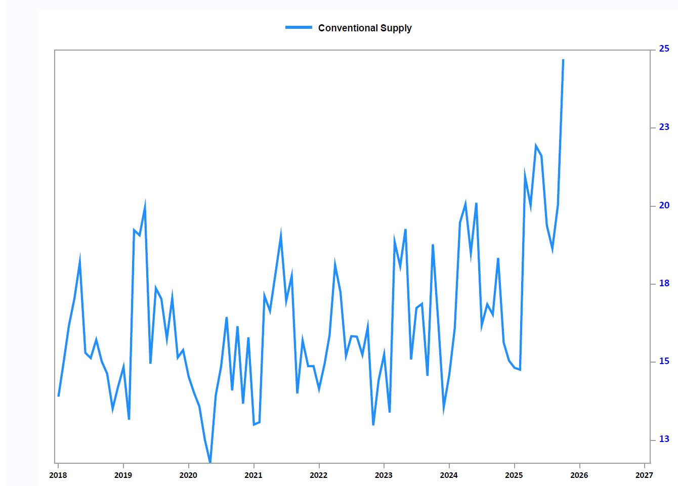
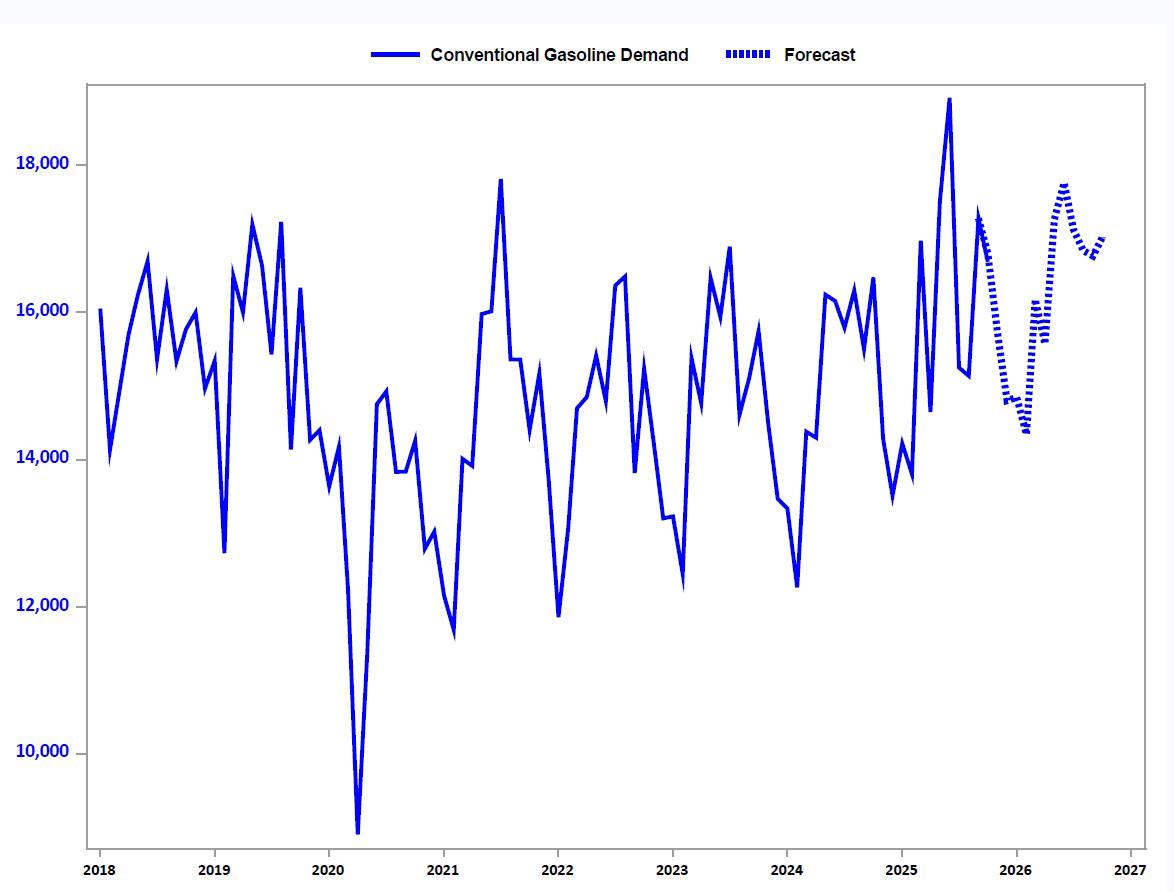
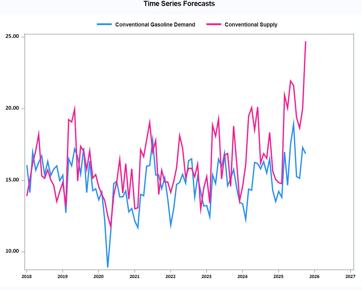
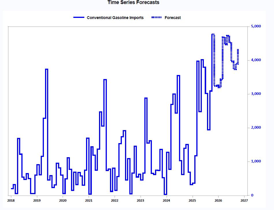
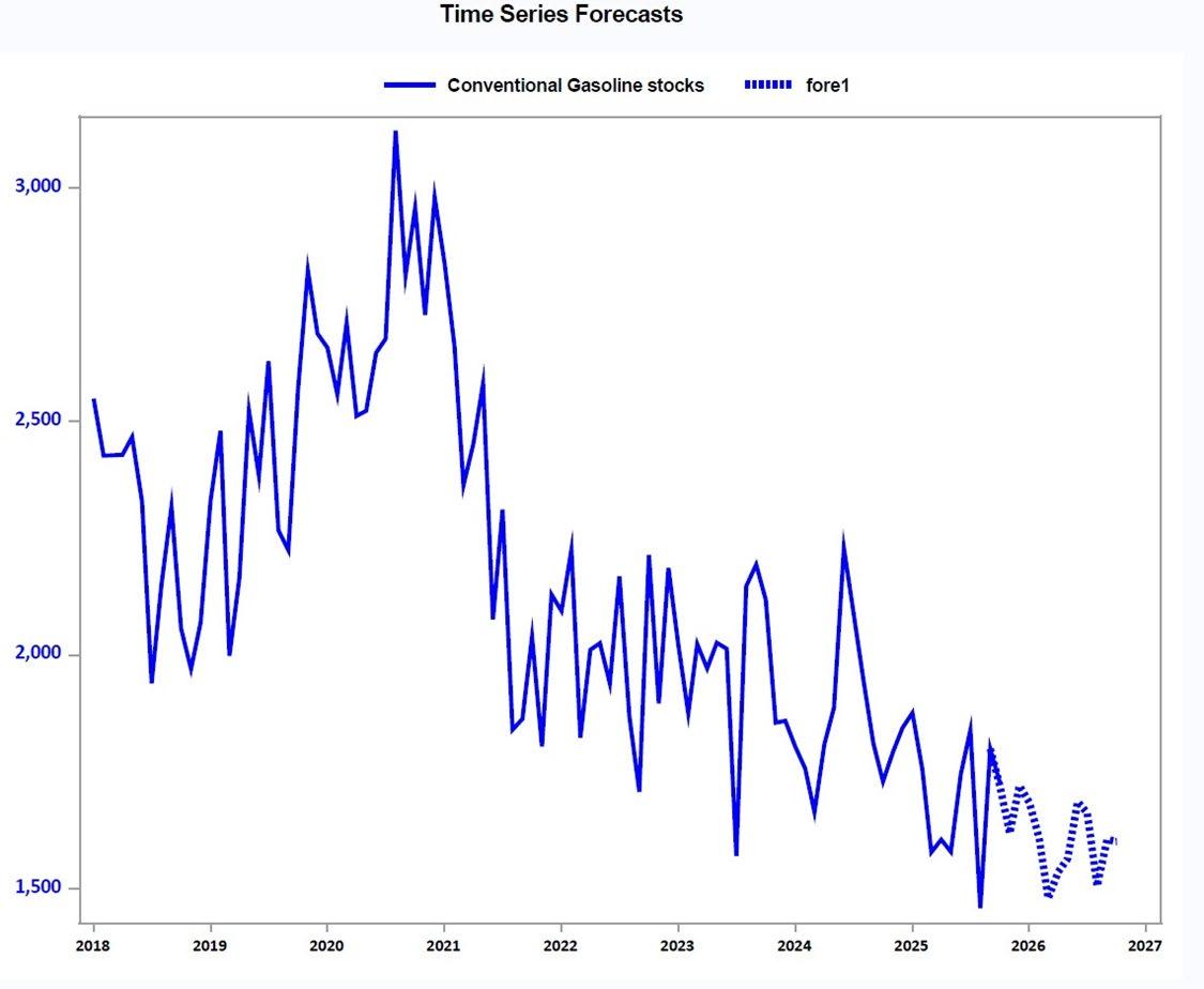
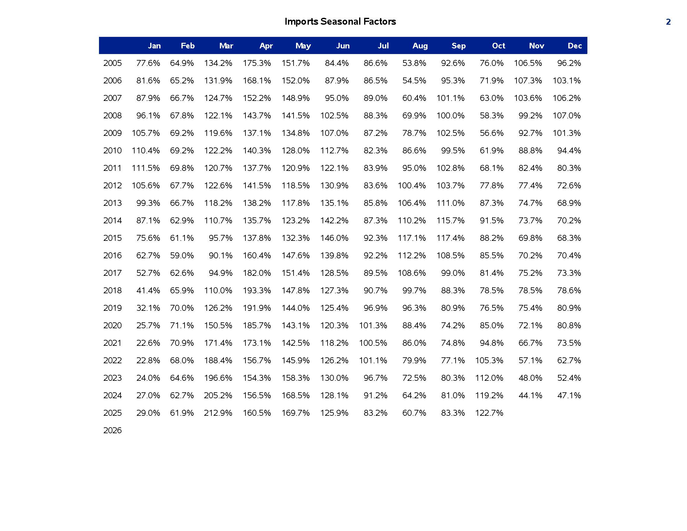
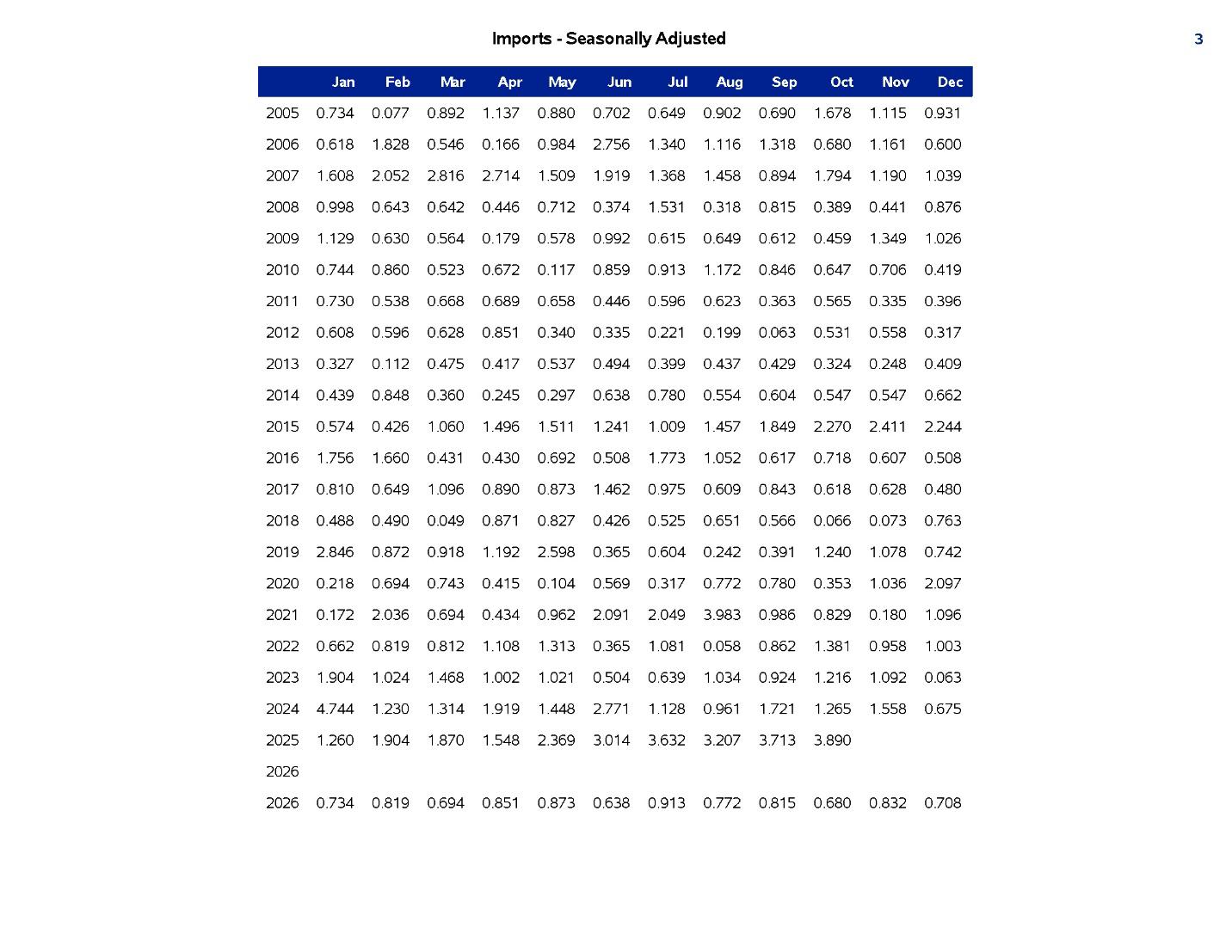
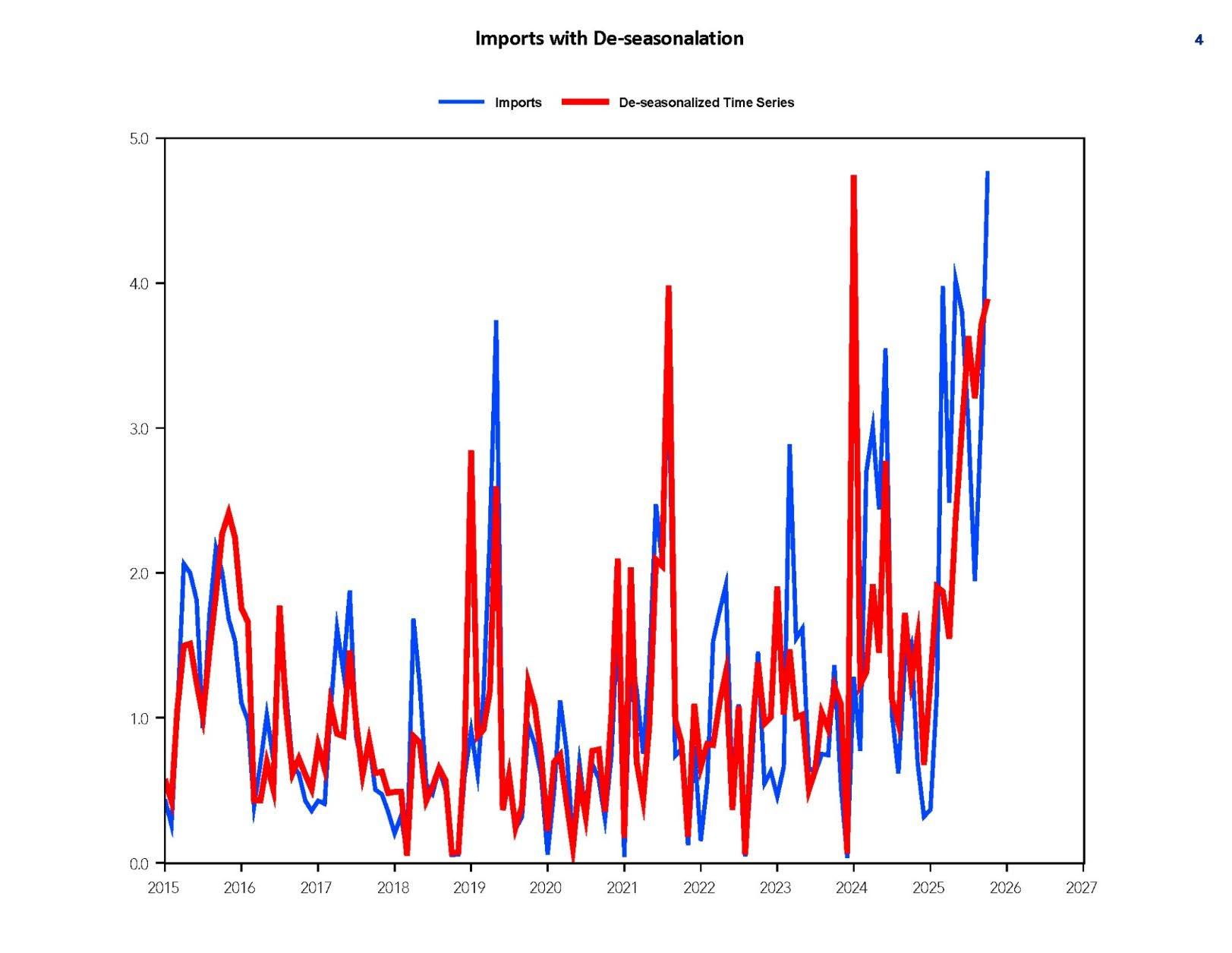
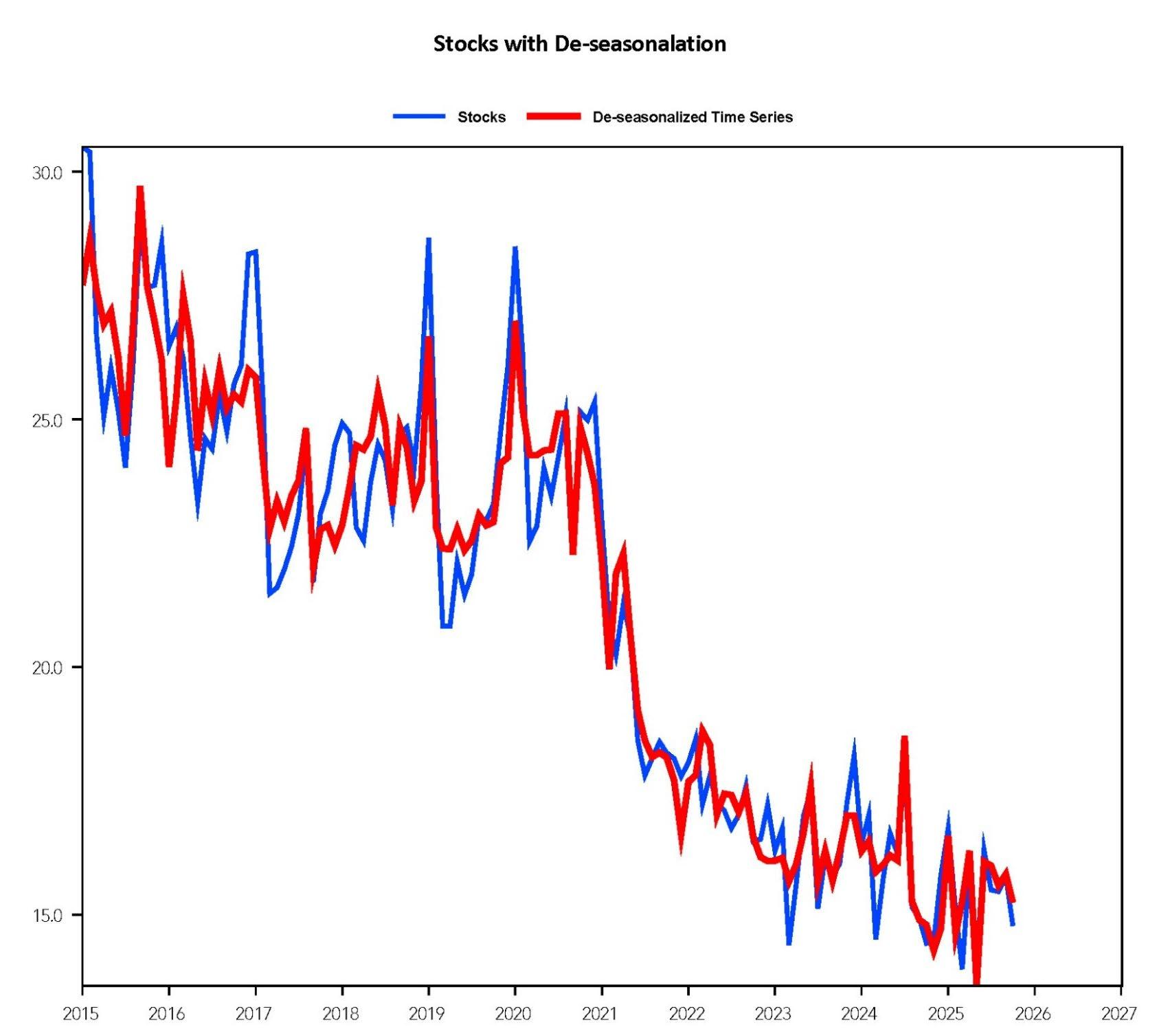
Times Series Plots: Conventional Gasoline Prices, Supply, Demand, Stocks, Imports
Time Series Plots: Conventional Gasoline Prices, Supply, Demand, Stocks, Imports
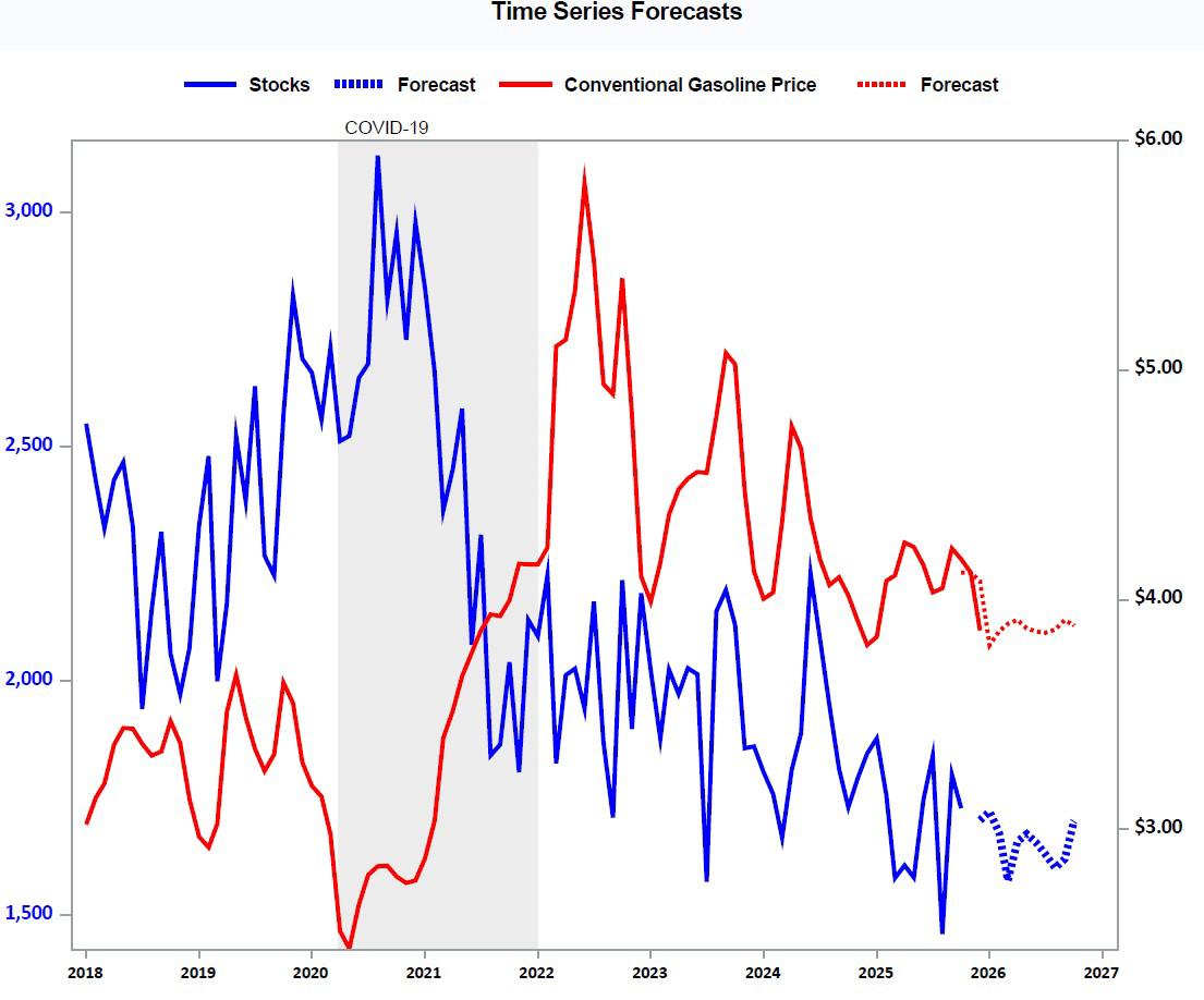
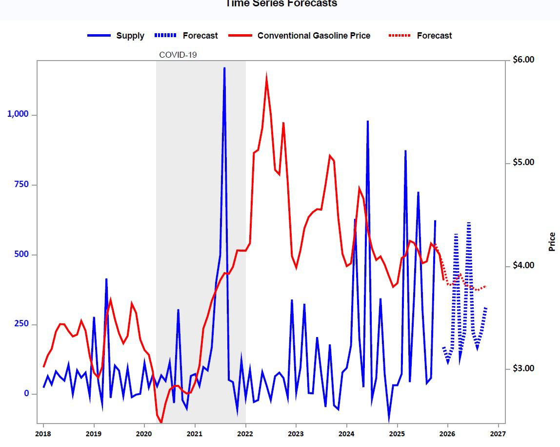
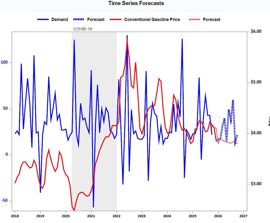
Conventional Regular Gasoline Prices, Production , Demand, Stocks
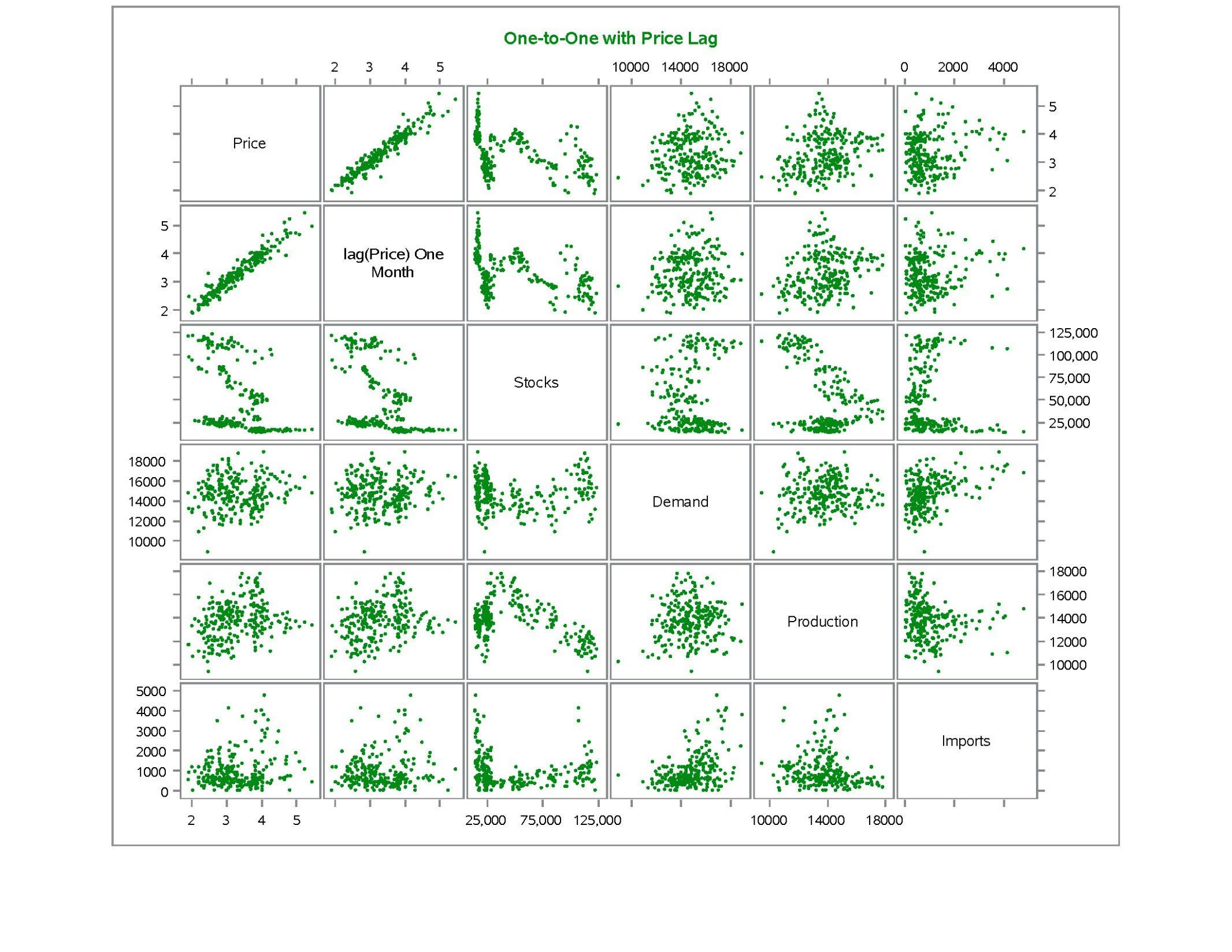
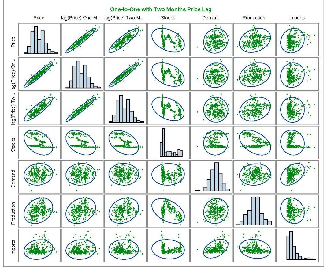
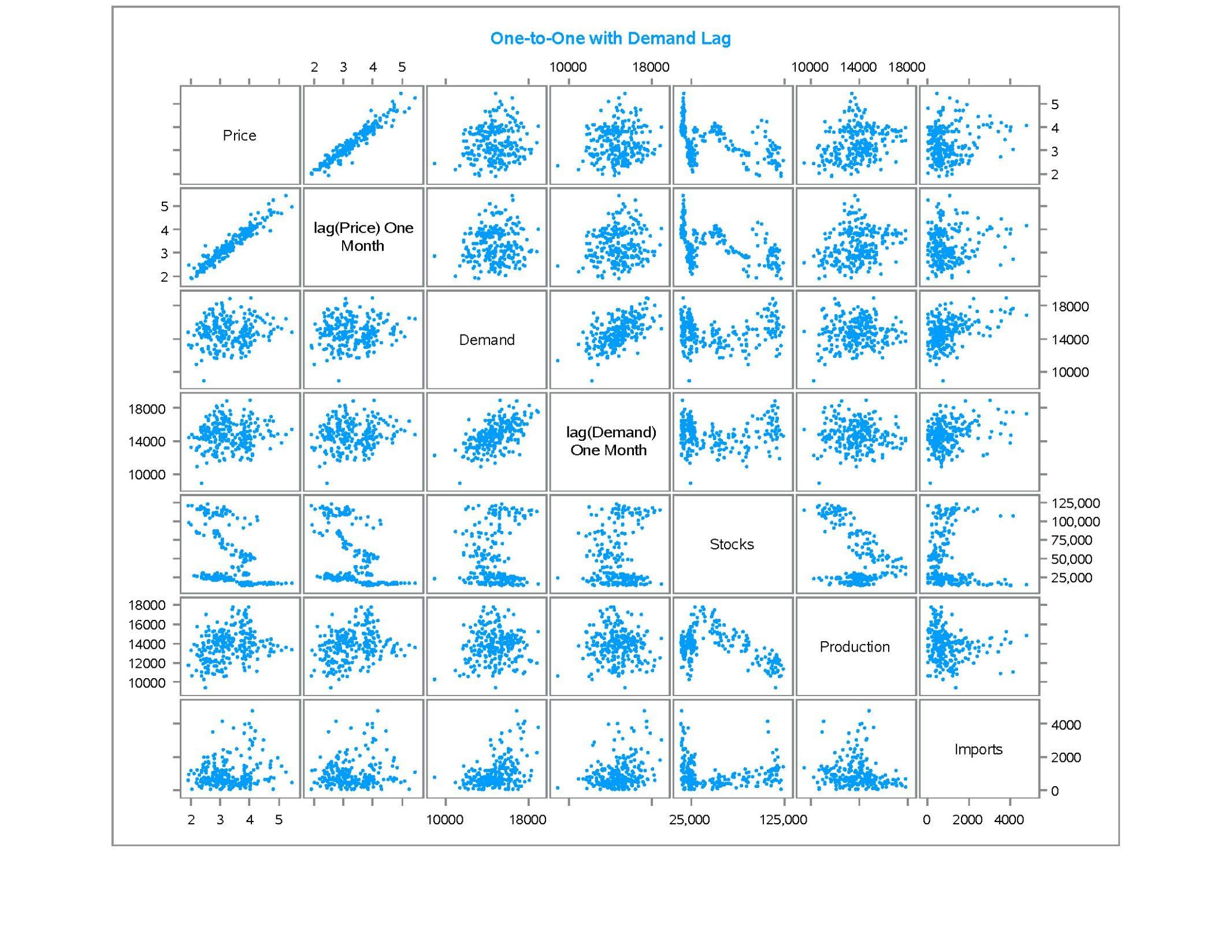
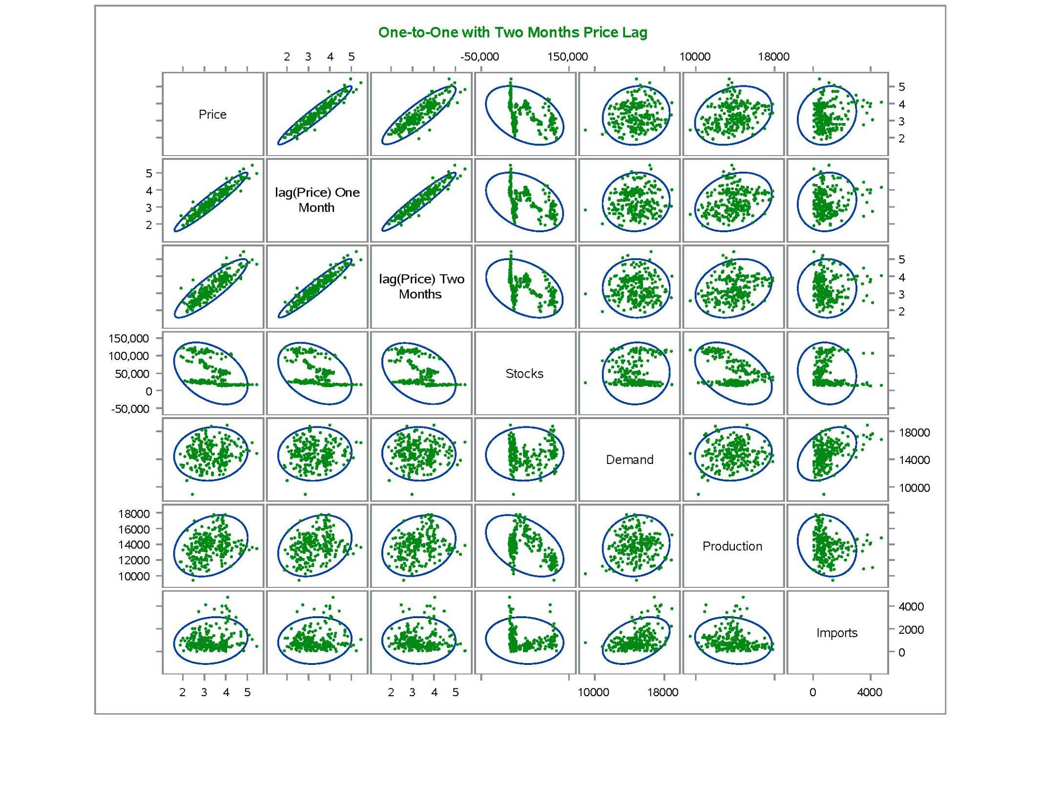
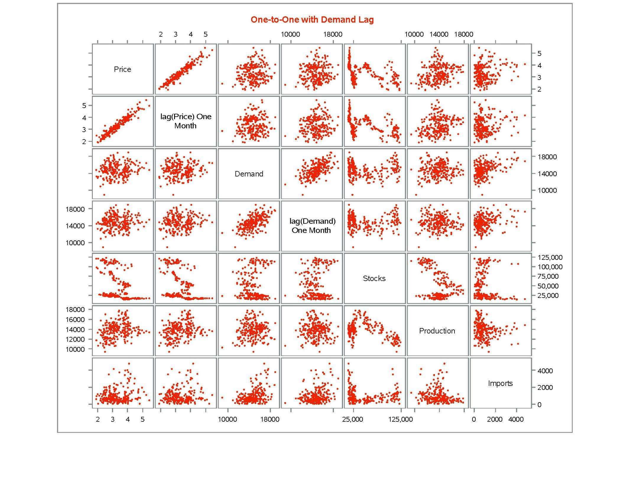
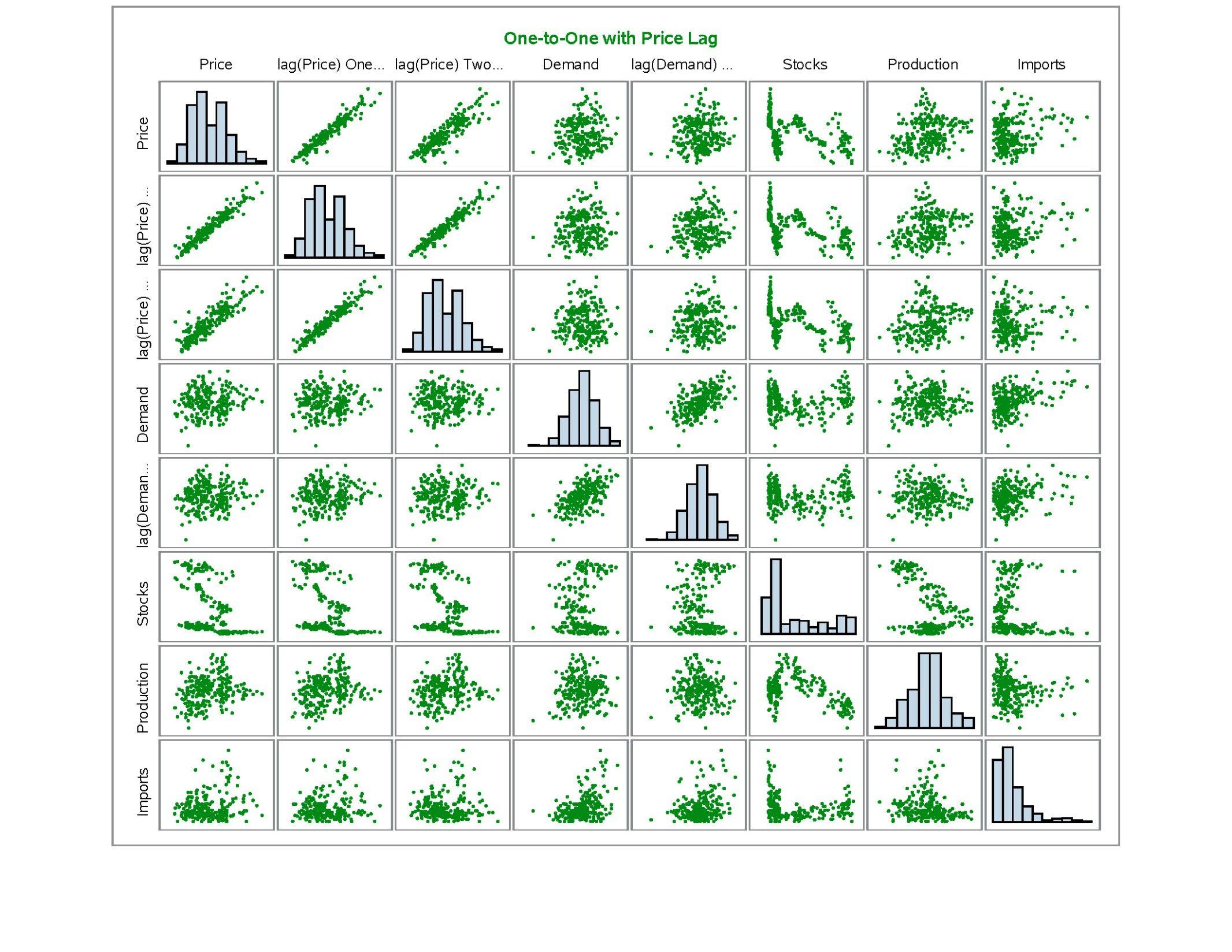
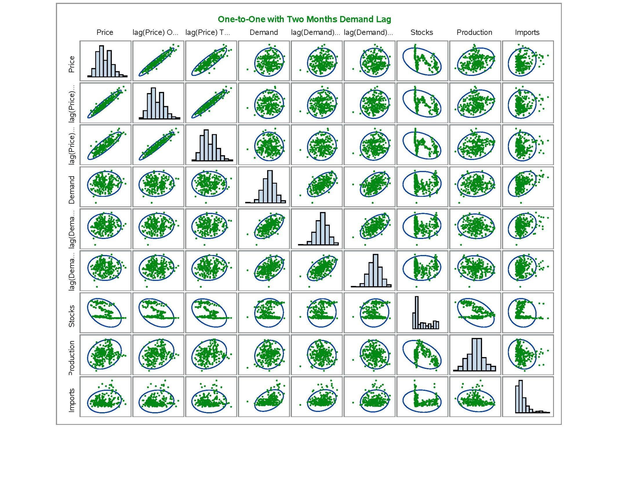
Bivariate statistics and analysis
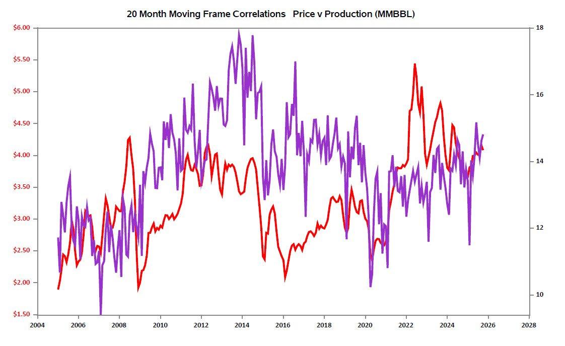
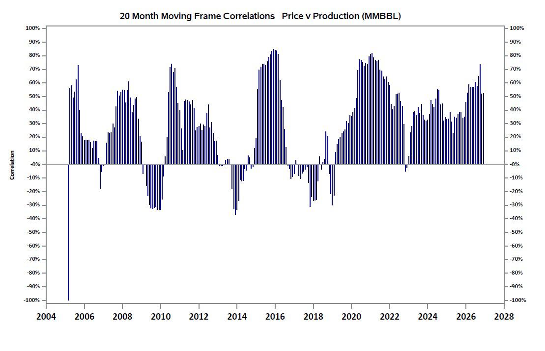
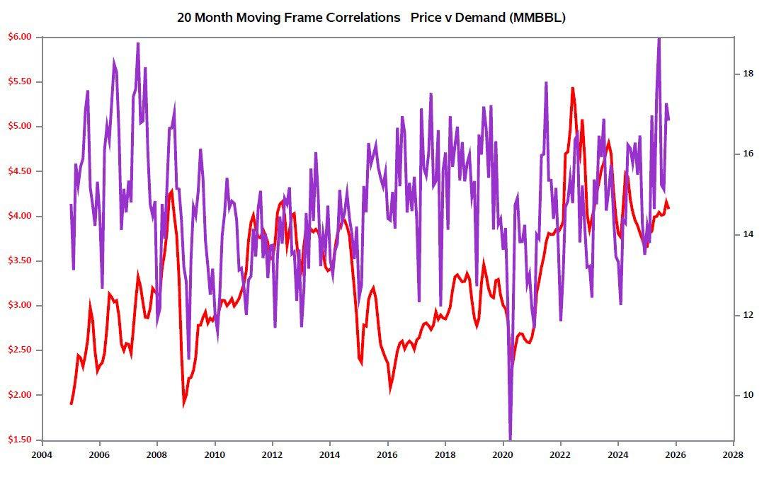
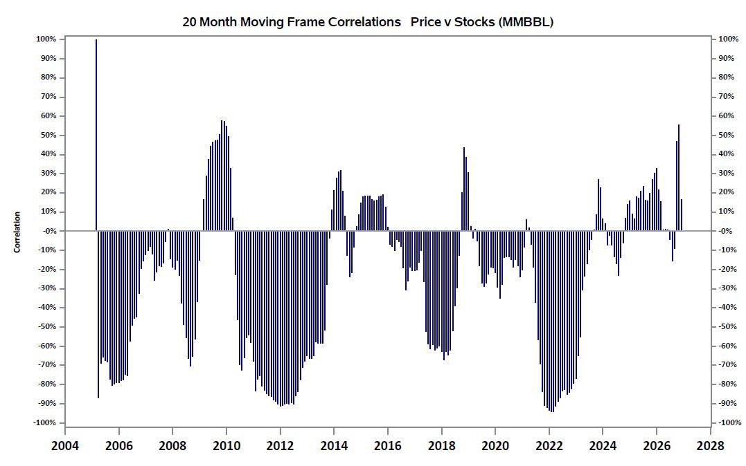
Correlations static/ Dynamic Correlations
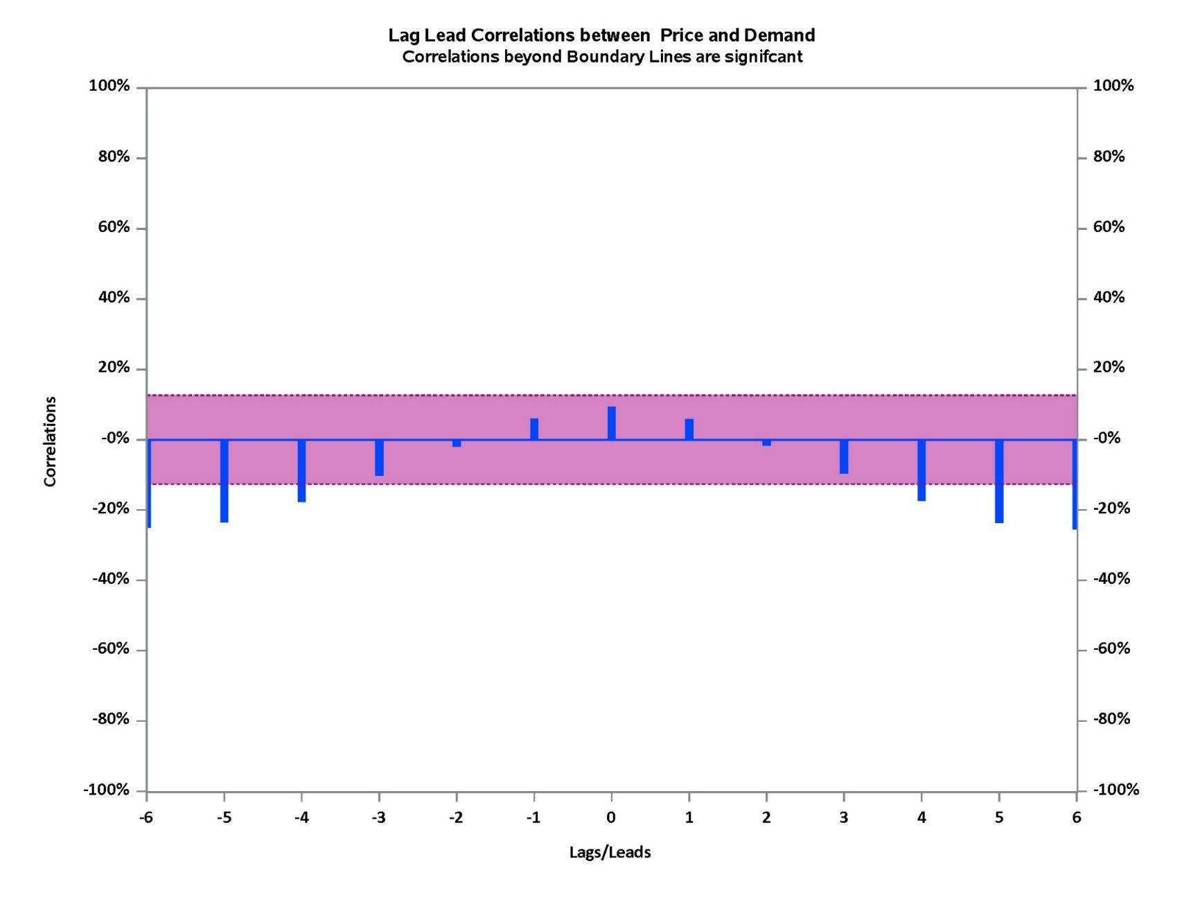
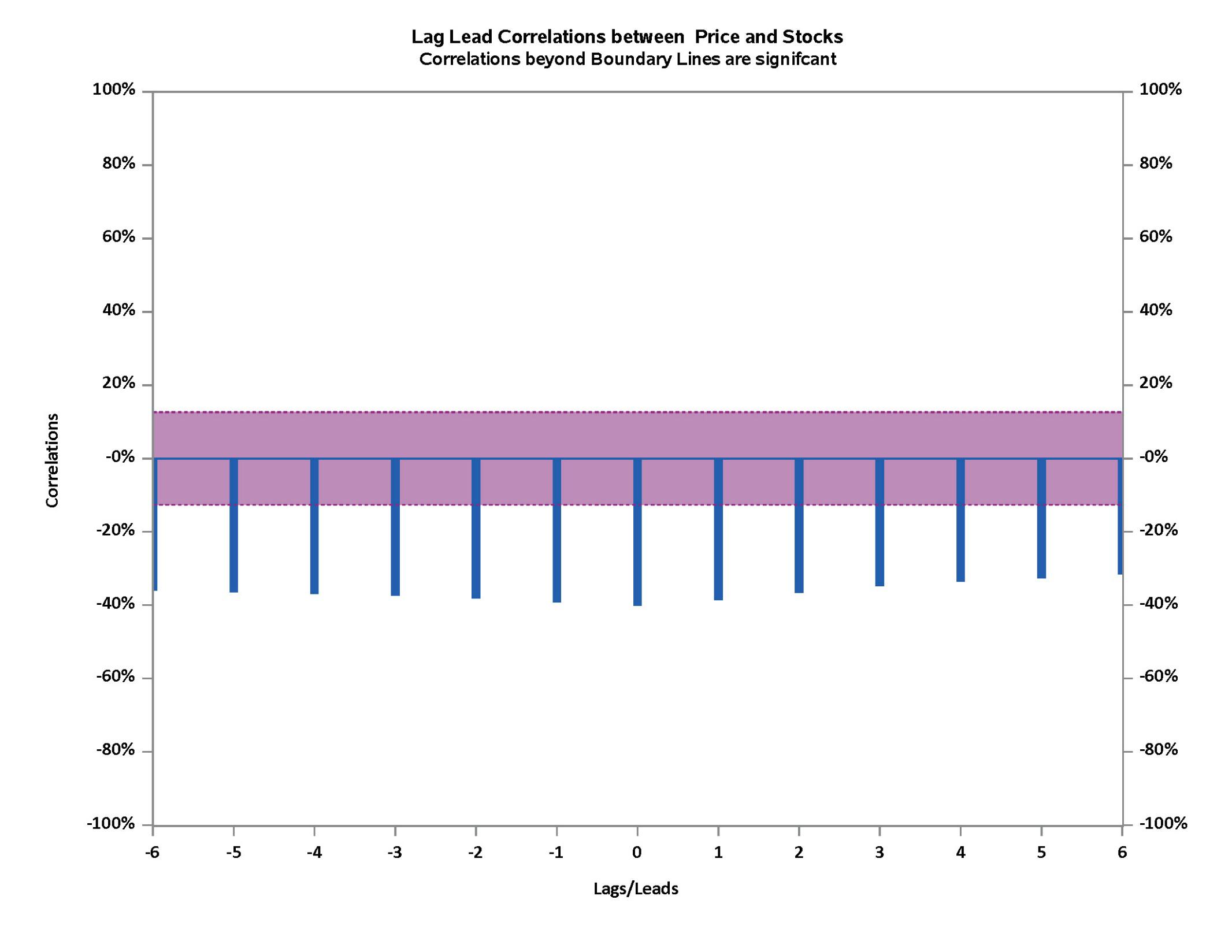
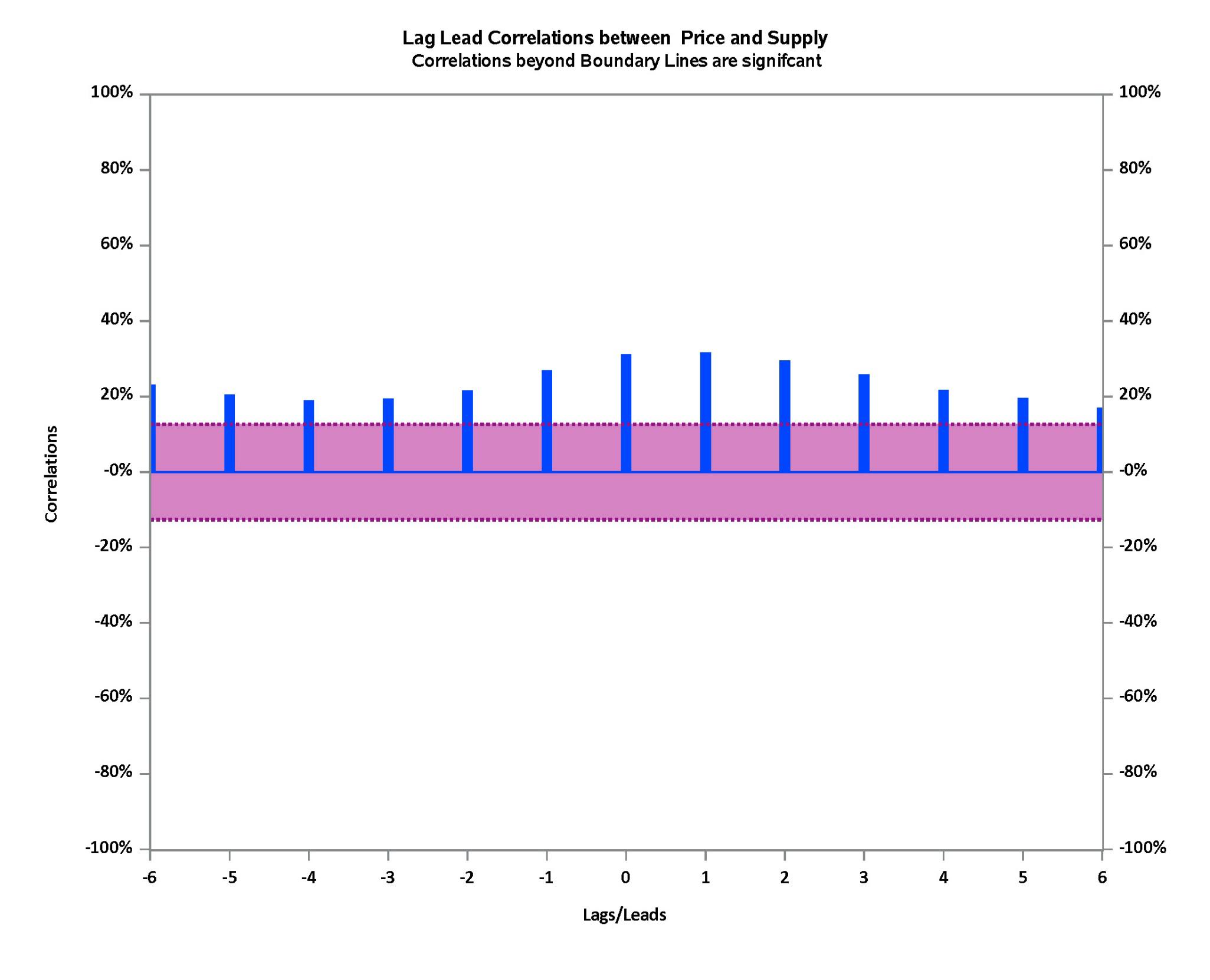
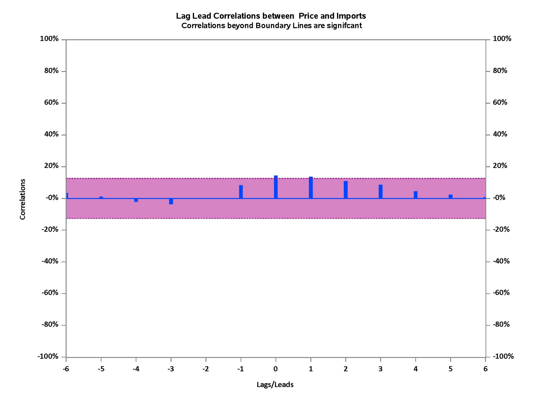
Cross Correlation Function Lead/Lag Analysis
Bivariate Forecast Models
tion Lead/Lag Analysis 01 West Coast (PADD5) Conventional Regular Gasoline
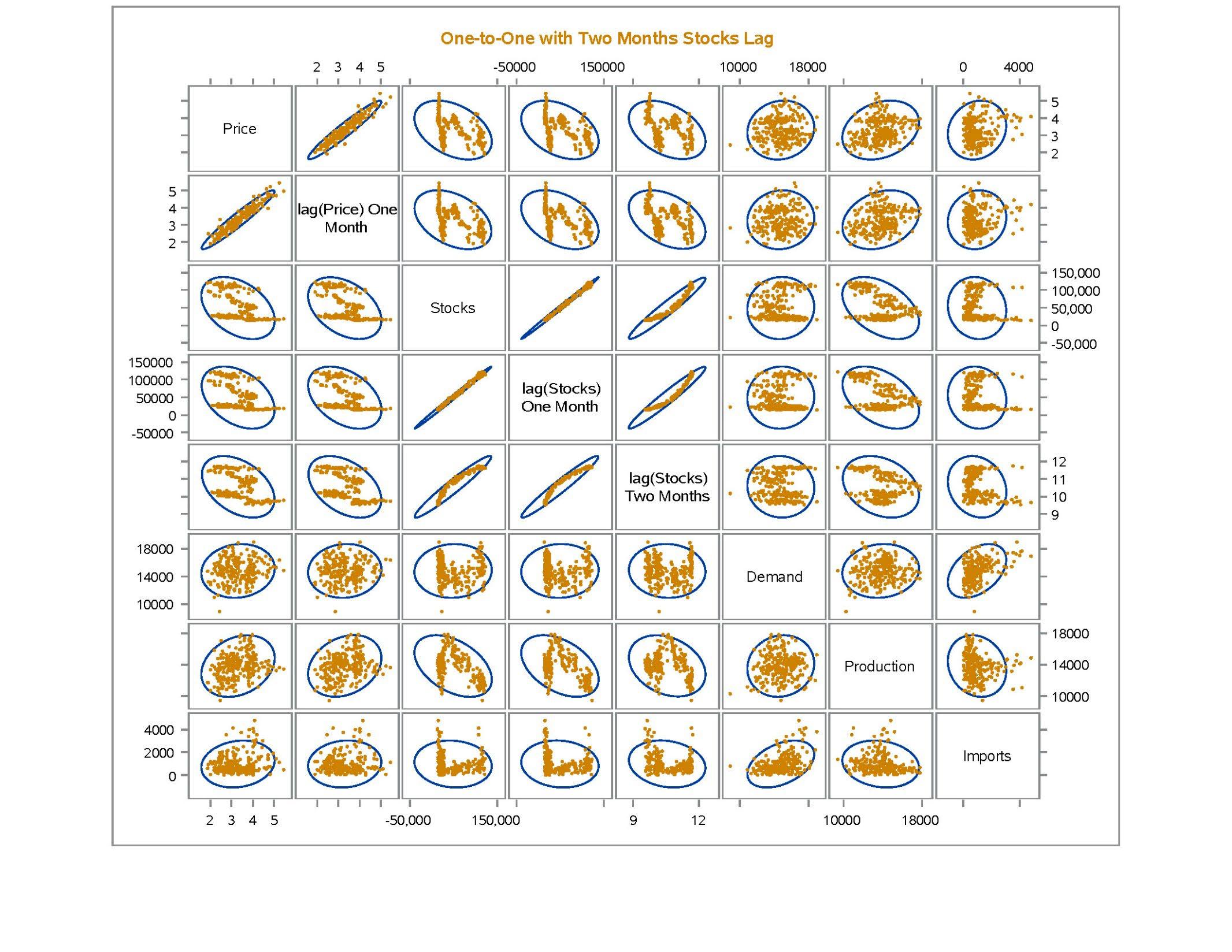
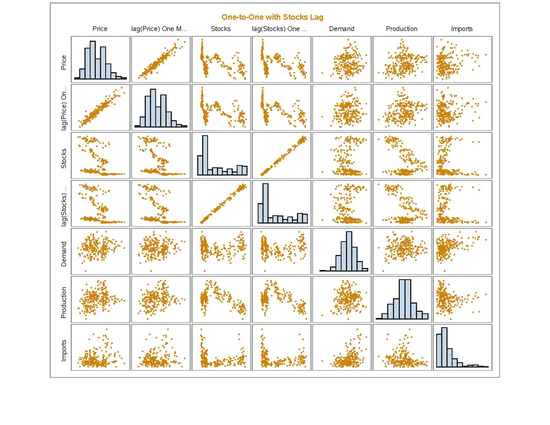
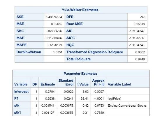
Bivariate with Stocks
Small in�luence from stocks, but strong in�luence from
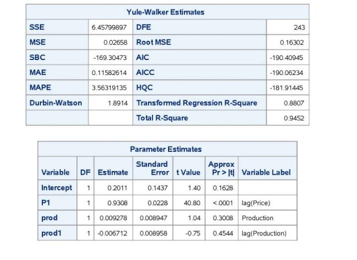
Bivariate with Production
Small in�luence from production, but strong in�luence from
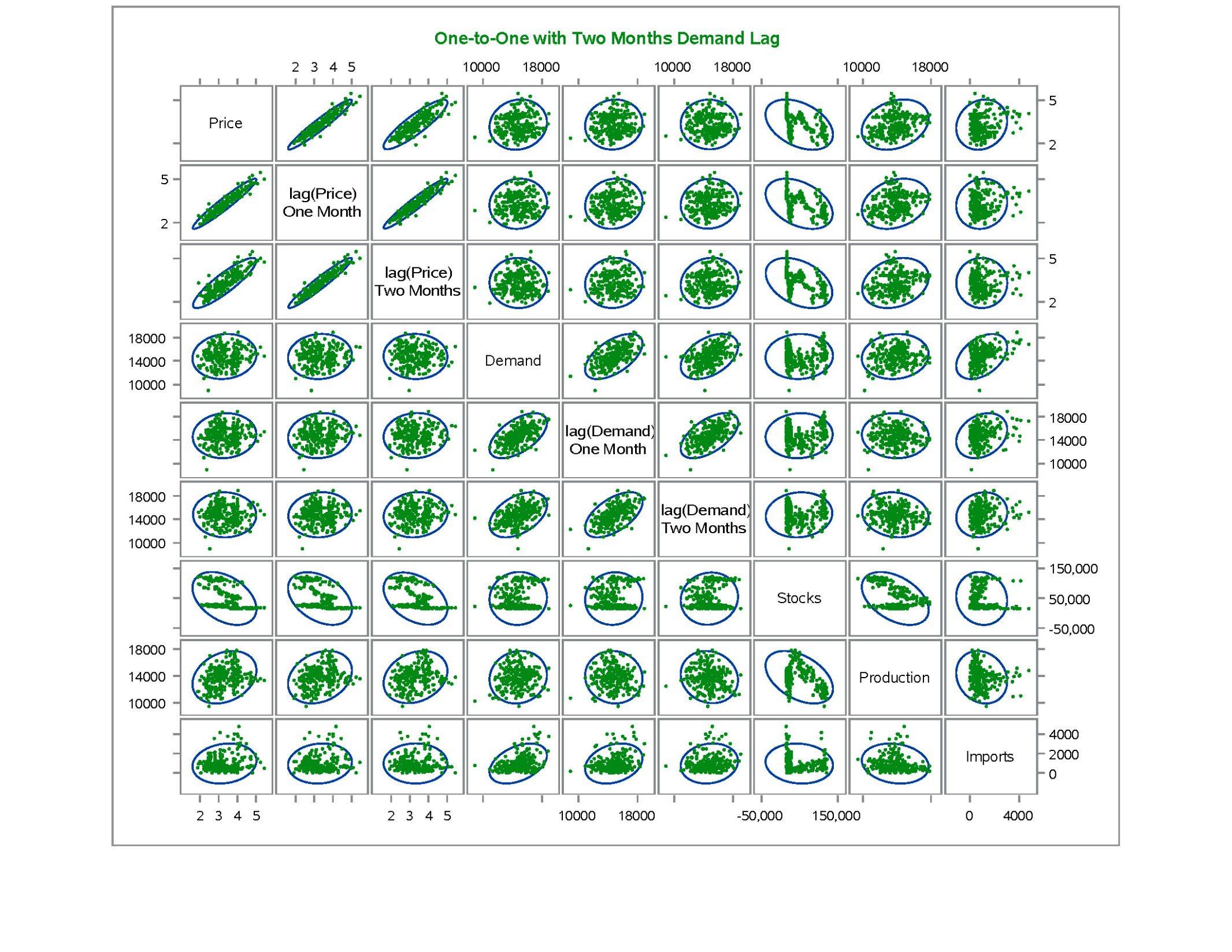
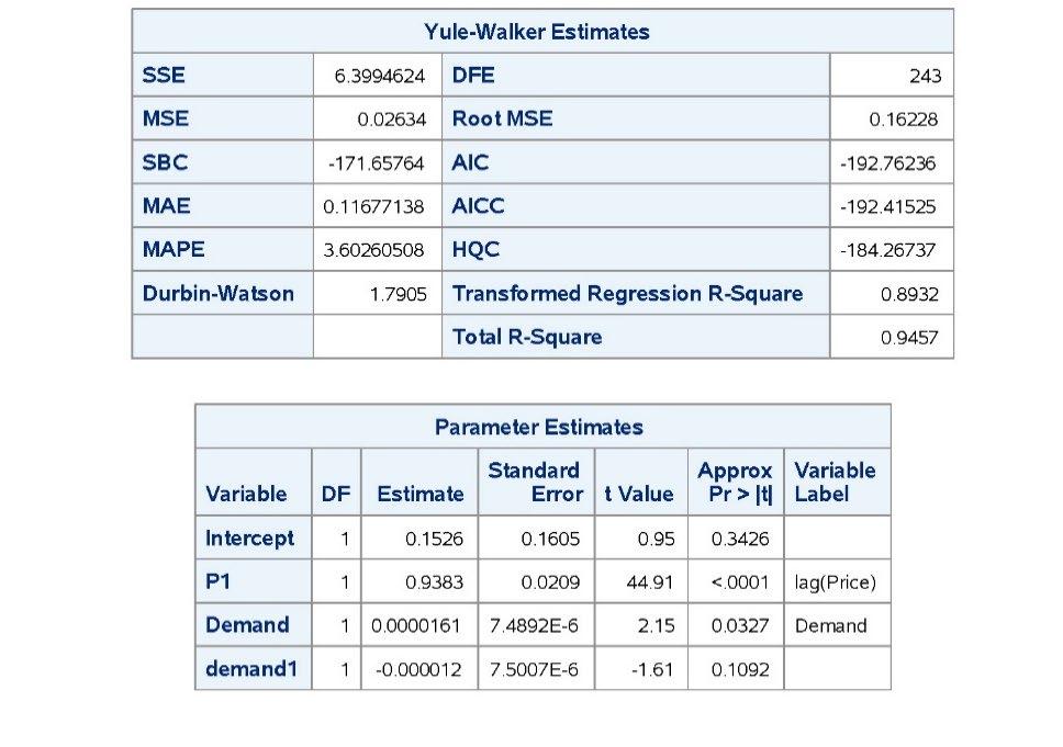
Bivariate with Demand
Small in�luence from production, but strong in�luence from
05 Accounting Identities and Economic Behavior 06 The Big Picture: What This System Is Doing
This project collects an internally consistent set of time series—covering production, demand (product supplied), prices, imports, re�inery activity, and inventories—and uses them to generate short- to medium-term forecasts for conventional gasoline.
Rather than relying on a single reduced-form price equation, the modeling framework re�lects the physical structure of the petroleum system:
• Re�iners produce gasoline subject to capacity, utilization, and crude inputs
• Consumers demand gasoline with strong seasonal and economic patterns
• Inventories absorb short-run imbalances between supply and demand
• Prices act as the adjustment mechanism tying the system together
This structure motivates both time-series forecasting and simultaneous-equation modeling.
\oline markets are not well described by a single autoregression. Production, demand,
A System rather than just one Equation
and inventories are jointly determined
Production responds to refinery margins, capacity utilization, and seasonality
Demand responds to price, income, and calendar effects
Inventories respond mechanically to the gap between production and demand
Estimating these relationships separately risks endogeneity bias. A system allows the model to treat price, production, demand, and stocks as endogenous, preserving economic logic while still exploiting the time-series dynamics in the data.
A system respects accounting identities and economic behavior at the same tim
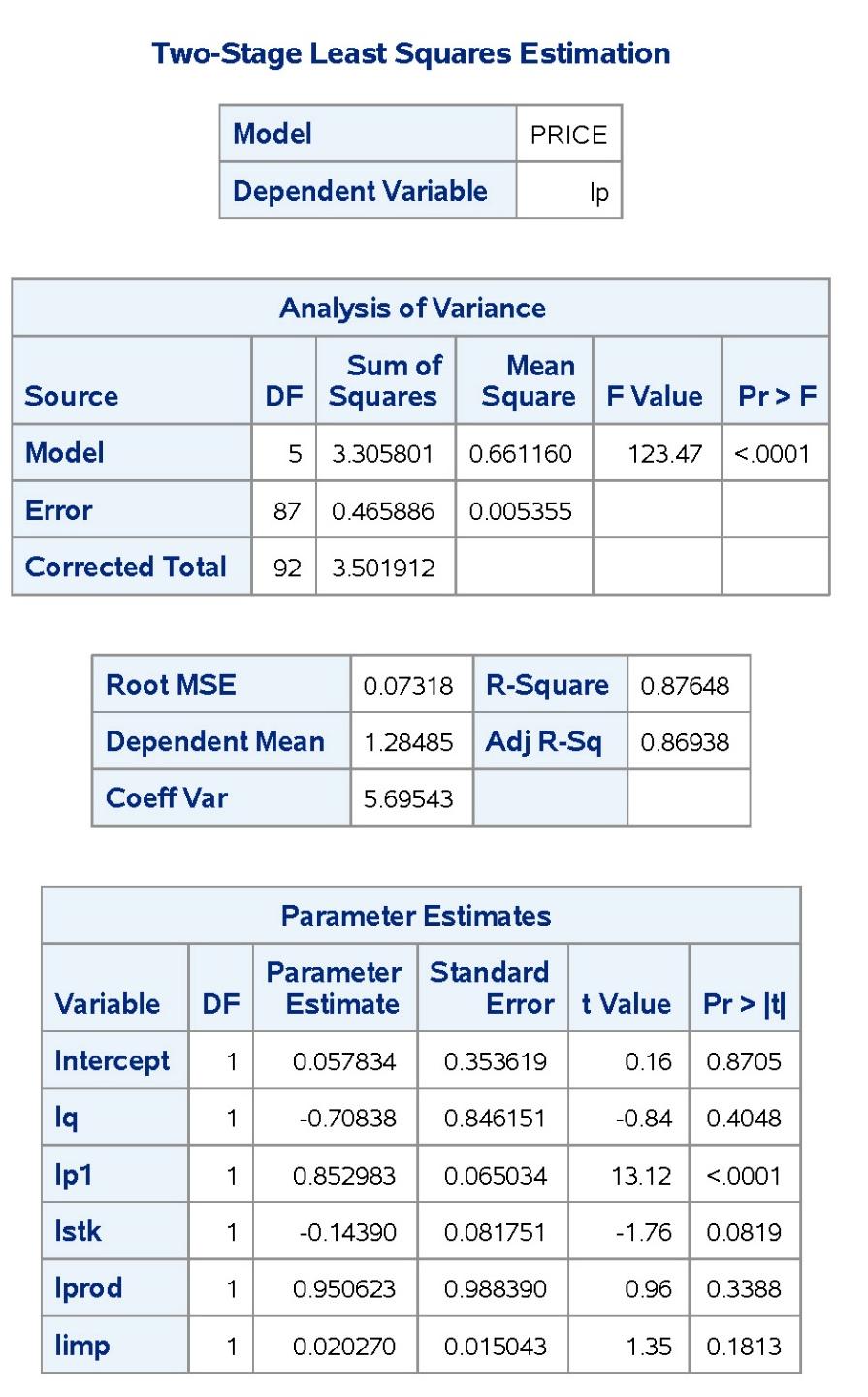
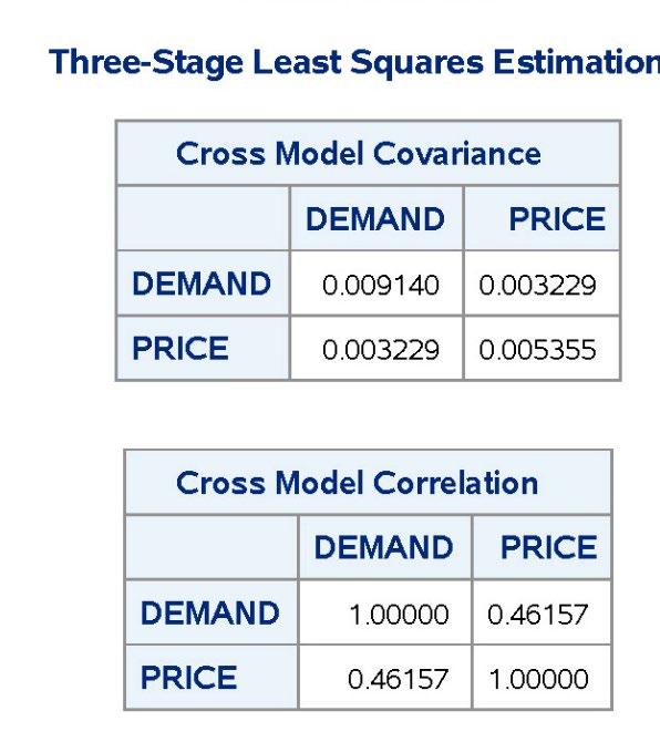
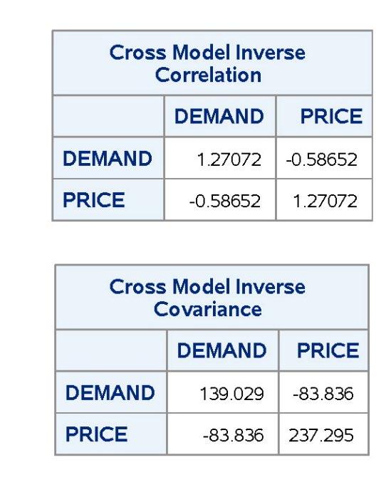
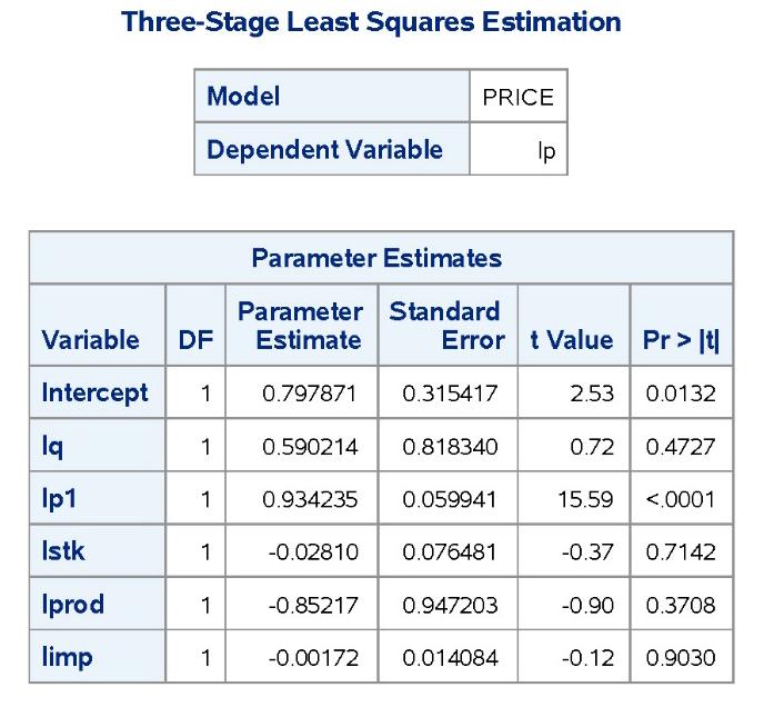
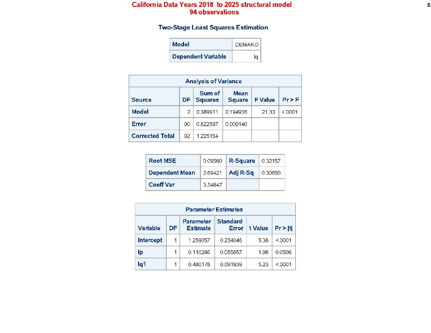
Two-stage least squares (2SLS) provides consistent equation-by-equation estimates, while three-stage least squares (3SLS) exploits cross-equation error correlation to improve efficiency.
Although coefficient magnitudes may differ modestly across estimators, the economic interpretation of the system is invariant.
3 Stage Least Squares
Stage 1: Use endogenous RHS variables on instruments, e.g. for demand equation, when replaced by a regression on demand.
Stage 2: Estimate the structural equation with instrumented regressors.
This is consistent even if the two error terms are correlated across equations
Stage 3 The same IV logic and uses an estimate of covariance to gain efficiency.
This system is consistent with that logic because price is being driven by: demand, stocks, and supply shifters
09
Reduced-Form Representation
Typical sign expectations:
• �������� < ���� short-run price elasticity of demand
• �������� < ����: more net production eases price pressure
• �������� < ����: more imports ease price pressure
Endogenous: ������������ , ������������
This identity underpins the model speci�ication and justi�ies the inclusion of inventories and supply variables as key determinants of price dynamic. Price and demand are jointly determined:
Demand depends on price
Price depends on demand
This means OLS would generally be biased because ������������ correlates with ������������ and ������������ correlates with ������������
Instrumental Variables
• Lags provide predetermined variation (common in dynamic simultaneous systems).
• Stocks and supply shifters move price directly and help identify demand response to price.
3 Stage Least Squares
Stage 1:
Regress endogenous RHS variables on Instrumental Variables. e.g. for demand equation, ������������ is replaced by �������� � ���� from a regression on �������� .
Stage 2:
Estimate the structural equation with instrumented regressors. This is consistent even if the two error terms ������������ and ������������ are correlated across equations
Stage 3
Then the same IV logic uses an estimate of ������������ (������������ , ������������ ) to gain ef�iciency.
This system is consistent with that logic because price is being driven by:
demand
Estimation
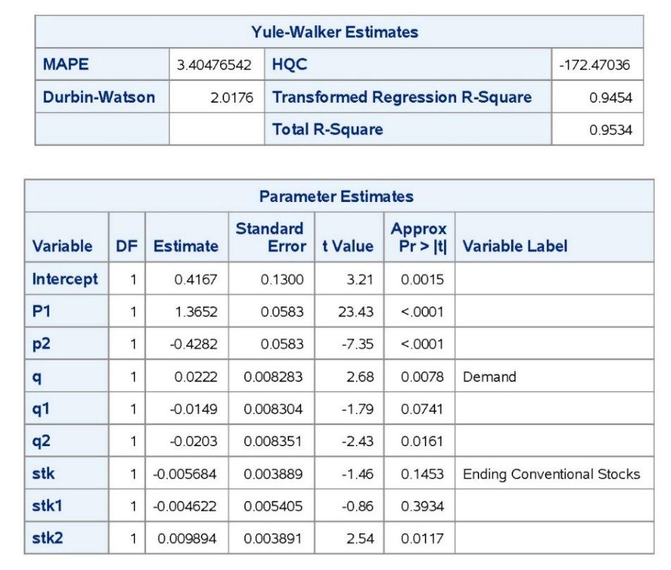
Model estimates the dynamic simultaneous system:
Demand (log product supplied)
Price (log retail price)
The system satis�ies both order and rank conditions, which is re�lected in the strong �irst-stage performance
12
Interpretation and Implications.
The Demand Equation
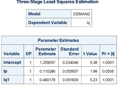
(a) Price elasticity
This is:
• Generally, not economically plausible (but high prob value)
• Statistically weak in the short run
Interpretation
West Coast gasoline demand is highly price inelastic at the weekly horizon. Consumers do not meaningfully adjust consumption in response to short-term retail price changes.
This directly explains why:
• Demand charts are smooth
• Price volatility does not feed back strongly into consumption
Persistence / habit formation
This is the dominant force in the demand equation.
Interpretation
• Roughly 48% of last week’s demand carries forward
• Demand dynamics are driven by habits, commuting patterns, and seasonality not spot prices
This explains why demand forecasts:
• Track seasonal patterns tightly
• Do not overreact to price spikes
Interpretation of the Price Equation
Strong price inertia
Retail gasoline prices are highly persistent.
Interpretation
• Prices adjust gradually
• Most week-to-week price movement is continuation, not re-optimization
This explains why:
• Price charts are smooth
• Forecasts do not show explosive oscillations
Demand effect on price
The sign �lips between 2SLS and 3SLS but remains economically small.
Interpretation
• Once persistence is accounted for, short-run demand shocks do not dominate price formation
• Prices respond more to inventory and supply conditions than to immediate consumption shifts
Inventories as the stabilizer
Higher stocks reduce price pressure.
Interpretation
Inventories act as a buffer stock
They absorb shocks before prices move materially
Interpretation
Imports respond endogenously to tight markets (price → imports)
oduction responds with lags and operational constraints
This explains why production appears smoother than demand or price in the charts.
This con�irms:
Demand and price shocks are not independent
Joint estimation improves ef�icient
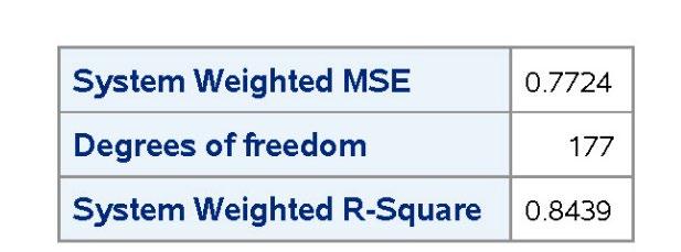
System weighted �������� = ����. ������������ indicates the system explains nearly all joint variation
Demand evolves slowly
Prices are even stickier
Inventories absorb short-run imbalance
Conclusions
The core economic result.
The system adjusts quantity → inventories → price not price → quantity.
In the West Coast gasoline market, short-run adjustment operates primarily through inventories and persistence rather than through immediate price–quantity feedback, yielding smooth, stable forecast paths even in the presence of seasonal demand �luctuations. The model’s charts and forecasts should be read as a validation of internal market coherence rather than as isolated projections.
Their signi�icance lies less in the level of any one series and more in whether the series move together in a way that respects market balance. By allowing prices, quantities, and stocks to adjust simultaneously, the system ensures that no single variable is forced to “do all the work.”
When demand strengthens, adjustment occurs through a combination of higher supply and inventory drawdowns rather than abrupt price jumps. When demand softens or production rises, inventories absorb the surplus, limiting downward price pressure.
This behavior is economically plausible. The absence of sharp reversals or explosive dynamics indicates that the system is adjusting through normal market channels rather than through forced, unstable corrections.
In practical terms, the forecasts re�lect how the gasoline market operates: re�iners, consumers, and storage jointly manage
First, short-run gasoline demand is highly persistent and relatively insensitive to contemporaneous retail price movements.
Second, retail prices are sticky: week-to-week movements contain a large “carry-over” component.
Third, inventories play the role of buffer stock—absorbing supply and demand shocks so that the market balances through stocks before it balances through price. These mechanisms explain why the forecast paths (and the diagnostics shown in the exhibits) are stable: the model’s adjustment channel is inventories and gradual price response rather than an unstable price–quantity feedback loop.
The core economic result of this modeling is that
Quantity → Inventories → Price
NOT Price → Quantity
In the West Coast gasoline market, short-run adjustment operates primarily through inventories and persistence rather than through immediate price–quantity feedback, yielding smooth, stable forecast paths even in the presence of seasonal demand �luctuations.
The model’s charts and forecasts should be read as a validation of internal market coherence rather than as isolated projections. Their signi�icance lies less in the level of any one series and more in whether the series move together in a way that respects market balance.
By allowing prices, quantities, and stocks to adjust simultaneously, the system ensures that no single variable is forced to “do all the work.” When demand strengthens, adjustment occurs through a combination of higher supply and inventory drawdowns rather than abrupt price jumps. When demand softens or production rises, inventories absorb the surplus, limiting downward price pressure.
This behavior is economically plausible. The absence of sharp reversals or explosive dynamics indicates that the system is adjusting through normal market channels rather than through forced, unstable corrections. In practical terms, the forecasts re�lect how the gasoline market actually operates: +re�iners, consumers, and storage jointly manage. First, short-run gasoline demand is highly persistent and relatively insensitive to contemporaneous retail price movements. Second, retail prices are sticky: week-to-week movements contain a large “carry-over” component. Third, inventories play the role of buffer stock—absorbing supply and demand shocks s These mechanisms explain why the forecast paths (and the diagnostics shown in the exhibits) are stable: the model’s adjustment channel is inventories and gradual price response rather than an unstable price–quantity feedback loop.
Suggestions for Further Research
The current framework provides an internally consistent representation of the West Coast gasoline market, but several extensions could deepen both its explanatory power and practical usefulness.
First, future work could explicitly model inventory decision-making rather than treating stocks as a predetermined state variable. Allowing inventories to follow an optimizing or target-adjustment process would strengthen the structural interpretation of the buffer-stock mechanism identi�ied here.
Second, the system could be expanded to incorporate re�inery utilization and capacity constraints. Re�inery operations are inherently nonlinear and subject to maintenance cycles, outages, and regulatory requirements, all of which may affect supply responsiveness during periods of market stress.
Third, disaggregation by gasoline grade or formulation, particularly reformulated versus conventional gasoline—could reveal heterogeneous adjustment dynamics that are masked in aggregate speci�ications. This is especially relevant for California markets with distinct regulatory regimes.
Fourth, incorporating expectations or forward-looking price measures, such as wholesale or futures prices, could improve identi�ication of pricing behavior and help distinguish cost pass-through from demand-driven price movements.
Finally, extending the model to a regional or multi-PADD system would allow explicit modeling of inter-regional �lows and arbitrage dynamics, providing a richer framework for analyzing supply disruptions, policy changes, or transportation constraints.
Together, these extensions would build on the core insight of the current analysis—that inventories and persistence dominate short-run adjustment—while expanding the model’s scope for scenario analysis and policy evaluation.
California Energy Demand Scenario Projections (AEP/UC Davis)
A scenario analysis from UC Davis/CEC modeling alternative futures for transportation fuel demand through mid-century, including gasoline demand implications under different socioeconomic and policy pathways.
Impacts of Gas Price on Vehicle Use & Emissions (ARB 2014 Technical Doc)
Analyzes price elasticities and consumption patterns in U.S. gasoline markets (useful for historical comparison).
EMFAC Modeling System (CARB)
While primarily an emissions model, EMFAC outputs are widely used to translate vehicle
haIf the EIA series doesn’t cover enough years for your needs, check the California Energy Commission’s (CEC) data portal which has additional gasoline statistical reports and sometimes detailed monthly or quarterly volumes.
California Gasoline Demand Elasticity Estimated Using Re�inery Outages presents statespeci�ic gasoline demand price elasticity estimates by exploiting variations in re�inery production and outages unique to California’s partially isolated fuel market. Estimates short- and long-run demand elasticities (≈ −0.25 short run; −0.60 long run) using instrumental variables. Relevant for analyzing how gasoline demand responds to price changes in a CARB-regulated market.
Forecasting California’s Energy Demand (2024)
Comprehensive Forecasting of California’s Energy Consumption: A Multi-Source and Sectoral Analysis Using ARIMA and ARIMAX Models. Though broader than gasoline alone, this analysis includes transportation energy trends and sectoral demand forecasts using time-series models.