We would like to express our gratitude to the following contributors to the second issue of the COSMOS Math Journal.
Editors
Dowon Her - Editor-in-Chief
Justin Wu - Managing Editor
Jinwoo Yang - Managing Editor
Writers
Brian Lee
Elias Brixen
Jihoo Lee
Doyeon Kim
Keiko Kaliman
Chaeyeoung (Amy) Lee
Chaewon (Wendy) Yang
Vincent Tjoa
Editor ’s Note
First of all, I would like to thank everyone who enjoyed the first issue of our first issue which was published in October Your support provided us with the motivation to create our second issue with an even better quality. For this issue, we have two special articles included. The first article is titled “1. How can we spread mathematical knowledge in a fun and applicable way? - A service trip to SMPN 161” This article shares the experience of three members of Cosmos teaching creative mathematics to middle school students in Indonesia The second article is titled “2 AP Statistics: A Beginner ’s Guide (And Why It’s Not That Hard),” which provides an overview of the AP Statistics course for anyone planning to take it next year. I hope you enjoy our articles and see you next year!
- Dowon Her, Editor-in-Chief
Contents
1. Special Articles
1. How can we spread mathematical knowledge in a fun and applicable way? - A service trip to SMPN 161 - Dowon Her
2. AP Statistics: A Beginner ’s Guide (And Why It’s Not That Hard) - Reyansh Sankhyan
2. Section 1: Pure Mathematics
1 The Mathematical Beauty of Nature: The Honeycomb Conjecture - Brian Lee
2 A Geometric Visualisation of the Sum and Product Rules - Elias Brixen
3. The Intricate Exploration of the Mandelbrot Set - Jihoo Lee
4. Gabriel's Horn Paradox: The Coexistence of the Finite and the InfiniteDoyeon Kim
3.
Section 2: Applied Mathematics
1 Analyzing Probability Theory in Corporate Risk Management - Keiko Kaliman
2. Application of Mathematics in Medical Imaging - Dowon Her
3 Where Will Crimes Occur: An Introduction to Kernel Density EstimationChaeyeoung (Amy) Lee
4. Analyzing Probability Theory in Corporate Risk Management - Chaewon (Wendy) Yang
5. Application of Statistical Analysis in Sports: The Effect of Launch Angle and Exit Velocity on the Success Rate of Home Runs - Jinwoo Yang
6. Binary and Hexadecimal Math in Microcontrollers - Vincent Tjoa
1. How can we spread mathematical knowledge in a fun and applicable way?: A service trip to SMPN 161 - Dowon Her
2. AP Statistics: A Beginner ’s Guide (And Why It’s Not That Hard) - Reyansh Sankhyan
Special Report: How can we spread mathematical knowledge in a fun and applicable way?
A service trip to SMPN 161
From April 21st to April 24th, three members of Cosmos, Dowon, Jinwoo, and Brian, and two other JIS students, Walter and Yi Chen, visited SMPN 161, a public middle school in Jakarta, for a LEAD Week project. The goal of our project was to address the question, “How can we spread mathematical knowledge in a fun and applicable way?” Instead of traditional teaching methods, we tried innovative and creative teaching methods that allowed students to experience mathematical concepts with their eyes, hands, and ears. We would like to introduce the activities we have done on each of the days
DAY 1
On day 1, students learned about the concept of volume and how to calculate the volume of different shapes. By measuring the dimensions of cylinders to calculate the volume and pouring water into them using a beaker, students could test out the formula for volumes in real life.
DAY 2
On day 2, we taught the concept of circles, pi, and ellipses through activities that involved entertainment, auditory experience, and teamwork. First, students were given a mission to walk around the campus to find the perfect circle, by measuring the value of the circumference divided by the diameter. Then this value was compared with the theoretical value of pi, 3.141592… A student who got 3.13 as their value won a chocolate pie as the prize.
Then, we introduced a fresh new perspective about the never-ending digits of pi by showing how each digit can be turned into a note, turning pi into beautiful music. Jinwoo played the violin, and Brian played the piano, together playing the digits of pi
As the last activity of the day, each student was given 10 digits of pi to memorize, for a total of 270 digits of pi as a team All students circled up in the classroom and called their digits one after another It was a moment in which the value of teamwork could be learned from mathematics
DAY 3
On day 4, we introduced the concept of Voronoi diagrams, and students learned how patterns in nature can be explained by mathematics We further taught them about the application of Voronoi diagrams by linking to their daily lives, such as ordering food from the closest restaurant on Gojek Then, students were provided with specific instructions to draw their own Voronoi diagrams using pen, markers, and colored pencils Many students were able to complete a unique and beautiful Voronoi diagram, and we were able to show the linkage between art and mathematics
DAY 4
On our last day, we started our lesson by asking why triangles are so commonly found in structures such as towers and bridges. We taught students the unique geometry of triangles compared to other shapes, allowing them to endure the most force possible. Using these learnings, students in groups of five competed to build the strongest tower using tape and spaghetti sticks. The strongest tower was able to hold 30 books until it finally collapsed.
To make the experience more memorable, we provided each student with a certificate with their name printed on it at the end of the four-day course.
Over the course of four days, we truly believe that we were able to answer the initial question that sparked this service project Although there were challenges in planning each lesson to be informative and fun at the same time, we believe that our hard work provided a shift in perspective regarding mathematics.
AP Statistics:
A Beginner ’s Guide (And Why It’s Not That Hard) - Reyansh Sankhyan (69249@jisedu.or.id)
Introduction
AP Statistics has a bit of a reputation Some people say it’s one of the easiest AP classes Others claim it’s confusing and full of weird formulas The truth? AP Stats is a mix of logic, common sense, and a few key formulas. If you’ve ever read a news article that said something like “80% of people prefer chocolate over vanilla,” you’re already dealing with statistics This guide will walk you through the major topics in AP Statistics and explain why it’s not as scary as you might think
1. Exploring Data: Describing Patterns and Distributions
Before you can analyze data, you need to know how to describe it This includes:
● Types of Data:
○ Categorical (like favorite colors, types of pets)
○ Quantitative (like height, test scores)
● Ways to Represent Data:
○ Histograms, box plots, dot plots, and scatterplots
● Measures of Center:
○ Mean (average)
○ Median (middle value)
● Measures of Spread:
○ Range (highest value - lowest value)
○ Standard deviation (how spread out the data is)
○ IQR (interquartile range, which helps with outliers)
● Shape of Distributions:
○ Symmetric, skewed left, skewed right
○ Normal distributions (the famous bell curve!)
Why This Isn’t Hard
Think of this as learning how to read a graph and summarize a bunch of numbers in a few simple stats If you can tell whether a test score is “way above average” or “about normal,” you’re already using these concepts
2. Collecting Data: Sampling and Experimentation
Good data doesn’t just fall from the sky. You have to collect it the right way.
● Types of Studies:
○ Observational studies (just watching what happens)
○ Experiments (actively changing something and measuring results)
● Sampling Methods:
○ Simple random sample (everyone has an equal chance of being chosen)
○ Stratified sample (dividing people into groups, then randomly choosing from each)
○ Cluster sample (randomly picking entire groups)
● Bias in Studies:
○ Selection bias (choosing the wrong sample)
○ Response bias (people lie or misunderstand the question)
○ Nonresponse bias (some people don’t respond at all)
● Experimental Design:
○ Control groups vs. treatment groups
○ Placebos (fake treatments to prevent bias)
○ Double-blind studies (neither the subjects nor the experimenters know who gets what)
Why This Isn’t Hard
You don’t need to do any complex math here. It’s mostly about understanding how data can be skewed or unreliable if collected poorly If you’ve ever ignored an online poll because you knew it wasn’t scientific, congrats you already get this
3. Probability: How Likely Is It?
Probability is about predicting the likelihood of different events.
● Basic Rules:
○ Probability is always between 0 and 1 (0% to 100%)
○ The sum of all possible outcomes = 1
● Independent vs. Dependent Events:
○ Independent: One event doesn’t affect another (flipping a coin)
○ Dependent: One event affects another (drawing cards without replacement)
● Addition Rule (for OR statements):
○ P(A or B) = P(A) + P(B) - P(A and B)
● Multiplication Rule (for AND statements):
○ P(A and B) = P(A) * P(B), if independent
● Conditional Probability:
○ The probability of A given that B already happened
● Normal Distributions & The 68-95-99 7 Rule:
○ 68% of data falls within 1 standard deviation of the mean
○ 95% falls within 2
○ 99 7% falls within 3
Why This Isn’t Hard
Probability is basically common sense with numbers. If you can answer “What are the chances of rolling a 6 on a die?” you already know how this works
4. Statistical Inference: Making Predictions
Once you have data, you can use it to make predictions about a larger population
● Confidence Intervals:
○ A range of values where we think the true value lies (e g , “We are 95% confident the average test score is between 80 and 90”)
● Margin of Error:
○ The range we allow for inaccuracy
● Hypothesis Testing:
○ Null hypothesis (H0): The assumption that nothing is happening (e g , “this drug does nothing”)
○ Alternative hypothesis (Ha): The assumption that something is happening (e g , “this drug works”)
○ P-value: If it’s low (usually <0 05), we reject H0
● Types of Errors:
○ Type I Error: False positive (rejecting H0 when it was true)
○ Type II Error: False negative (failing to reject H0 when it was false)
Why This Isn’t Hard
This is the part that seems tricky but isn’t bad when you break it down Most of it involves following a structured process and interpreting results. If you’ve ever said, “This study might be wrong because they didn’t test enough people,” you’re thinking like a statistician.
Why AP Stats Isn’t As Hard As You Think
1 Less Memorization, More Understanding
○ Unlike AP Calculus, AP Stats doesn’t require heavy memorization of formulas Most of them are provided on the exam It’s more about understanding concepts than raw calculations
2 No Super Complicated Math
○ The hardest math in AP Stats is algebra-level If you can handle fractions, percentages, and basic algebra, you’re fine.
3 It’s Everywhere in Real Life
○ From medical studies to political polls, statistics is everywhere. Once you start seeing it, you’ll find it easier to grasp
4 Calculator Does the Heavy Lifting
○ Most calculations are done using a graphing calculator (like the TI-84), so you don’t have to do complex calculations by hand
5 The AP Exam is Straightforward
○ The free-response questions follow a predictable pattern If you practice enough, you’ll see the same types of problems over and over again
Conclusion
AP Statistics isn’t a hard class it’s just different It’s about reasoning and interpretation more than computation If you approach it with an open mind, a bit of curiosity, and a willingness to practice interpreting data, you’ll do just fine Plus, it’s one of the most useful AP classes since stats are used everywhere, from science to business to everyday life. So, if you’re debating whether to take AP Stats, go for it! It’s way more manageable than you might think
Section 1: Pure Mathematics
1. The Mathematical Beauty of Nature: The Honeycomb Conjecture - Brian Lee
2. A Geometric Visualisation of the Sum and Product RulesElias Brixen
3. The Intricate Exploration of the Mandelbrot Set - Jihoo Lee
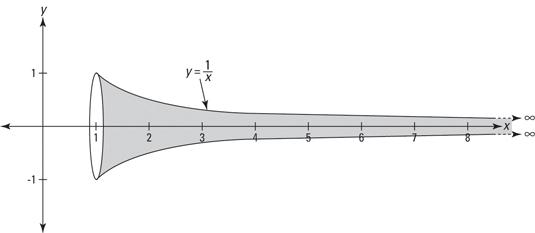
4. Gabriel's Horn Paradox: The Coexistence of the Finite and the Infinite - Doyeon Kim
The Mathematical Beauty of Nature - The Honeycomb Conjecture
By Brian Lee 72090@jisedu.or.id
Applied
Mathematics
Field of application: Patterns in nature
1 Introduction
Mathematics is often permeated into nature, optimizing conditions for the well-being and survival of living organisms One widely recognized example of the interplay between math and nature is the honeycomb conjecture Bees as a colony build a honeycomb, with beeswax, successfully creating an efficient storage system for eggs, larvae, and honey. A closer inspection shows that each honeycomb room forms a hexagonnearly 100% of them, in fact This article will explain the concept of the honeycomb conjecture, as well as analyzing the mathematical principle behind them
2 H. Conjecture - Optimization
First discussed by the people of ancient Greek and later proven by Thomas C. Hales in the late 1990s, the honey conjecture proposes that hexagon tiling is the most efficient way to separate a plane into spaces with equal areas, while minimizing the total perimeter
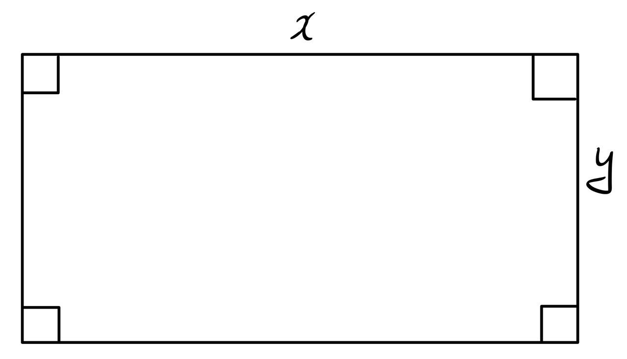
To begin with, we can make numerously different shapes using the same amount of length. Let’s assume that the given fixed length is 40 cm To use a rectangle as an example, if we assume the width as ‘x’cm and the length as ‘y’cm, the equation for the perimeter can be written as 2 (� + �) = 40 ��
By modifying this equation, , (� + �) = 20 we can see that the relationship between the width and length is � = 20 � Subsequently, the area of the rectangle can be written as If we substitute the � = � � equation above, the area can also be written as
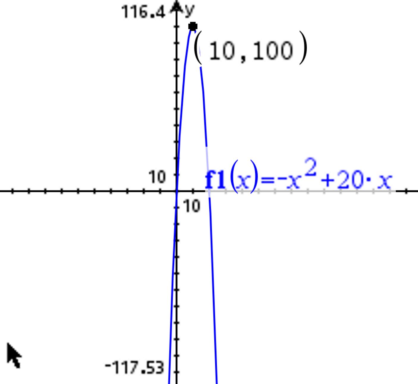
To � = � · (20 �) = 20� � 2 differentiate the equation to determine the maximum area, . �� �� = 20 2�
. Hence, . 20 2� = 0 � = 10 ��
The maximum area of a rectangle is when ; in 100��2 � = 10 ��, � = 10 �� other words, when the rectangle is a square, a regular polygon. Similarly, we can mathematically prove that the maximum area
of each shape is when it exists in the form of a regular polygon
3 H. Conjecture - Geometry
Now that we know regular polygons produce the maximum area, we must determine the type of regular polygon, using the same amount of length, that produces the greatest area. This time, let’s assume that the given fixed length is 30 cm Numerous different kinds of polygons can be created with different numbers of sides.
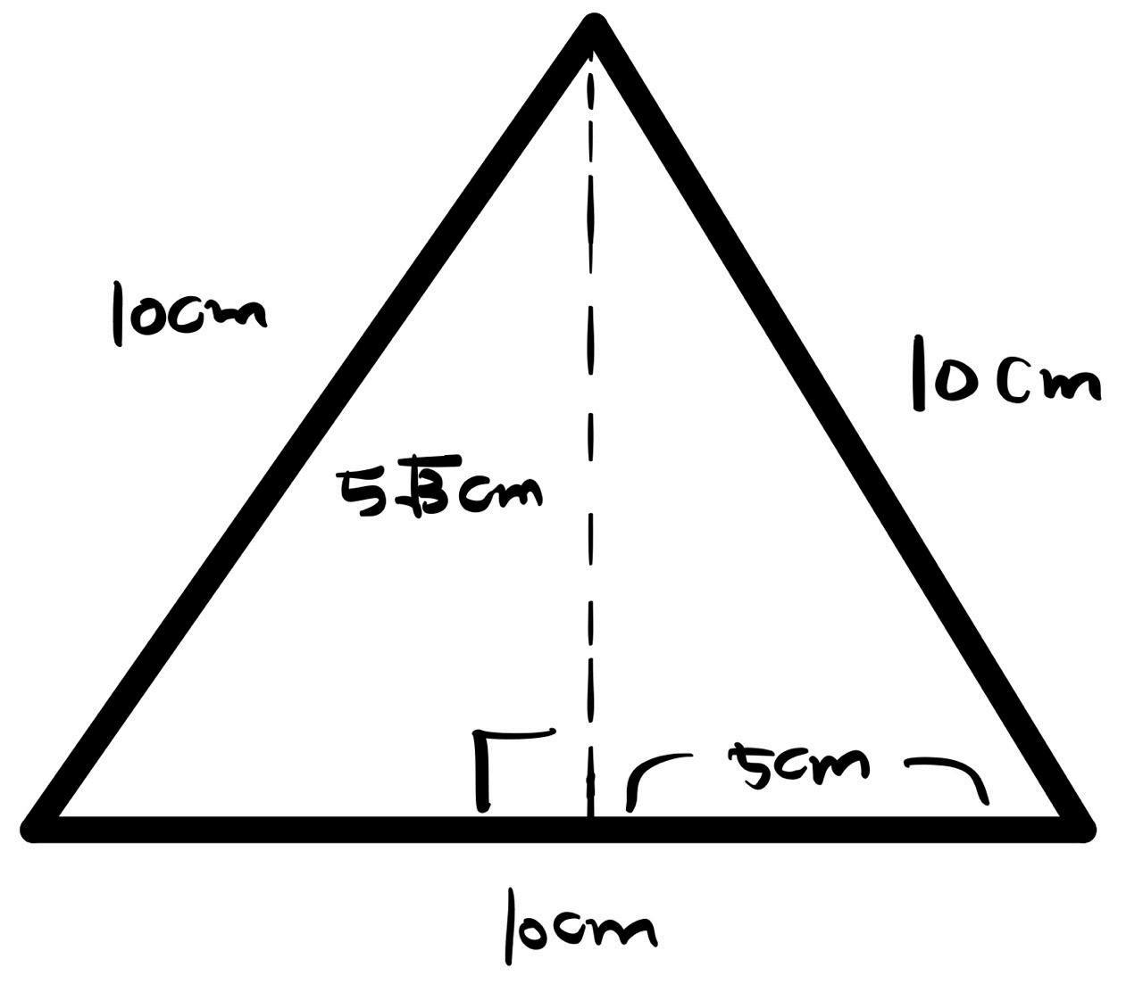
The area of the equilateral triangle, with a perimeter of 30 cm, can be determined as 10 5 3 1/2 ≃ 43 3 �� 2
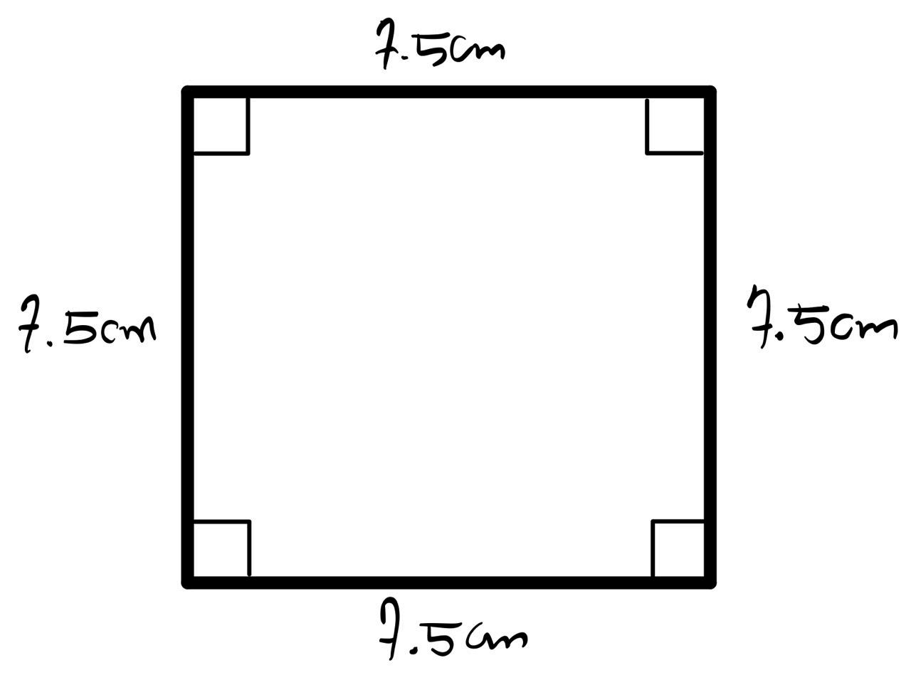
Next, the area of a square, with a perimeter of 30 cm, can be determined as 7 5 · 7 5 ≃ 56 3 �� 2
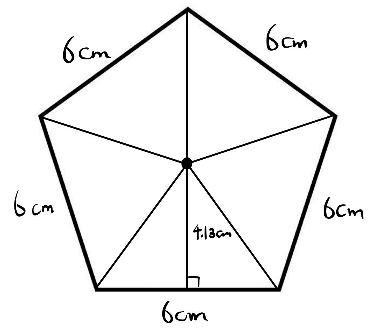
Lastly, the area of a pentagon, with a perimeter of 30 cm, can be determined as . (6 4 13 1 2 ) 5 ≃ 62 0 �� 2
In sum, we can see a relationship that, given the equal length of perimeter, the area of a polygon increases as the number of sides increases. If the number of sides increases infinitely, the polygon will eventually become a circle So, in order to maximize the area, should the honeycomb be composed of circles? However, although this theory may be true based on individual polymers, the maximum area upon multiple polymers is a completely different story
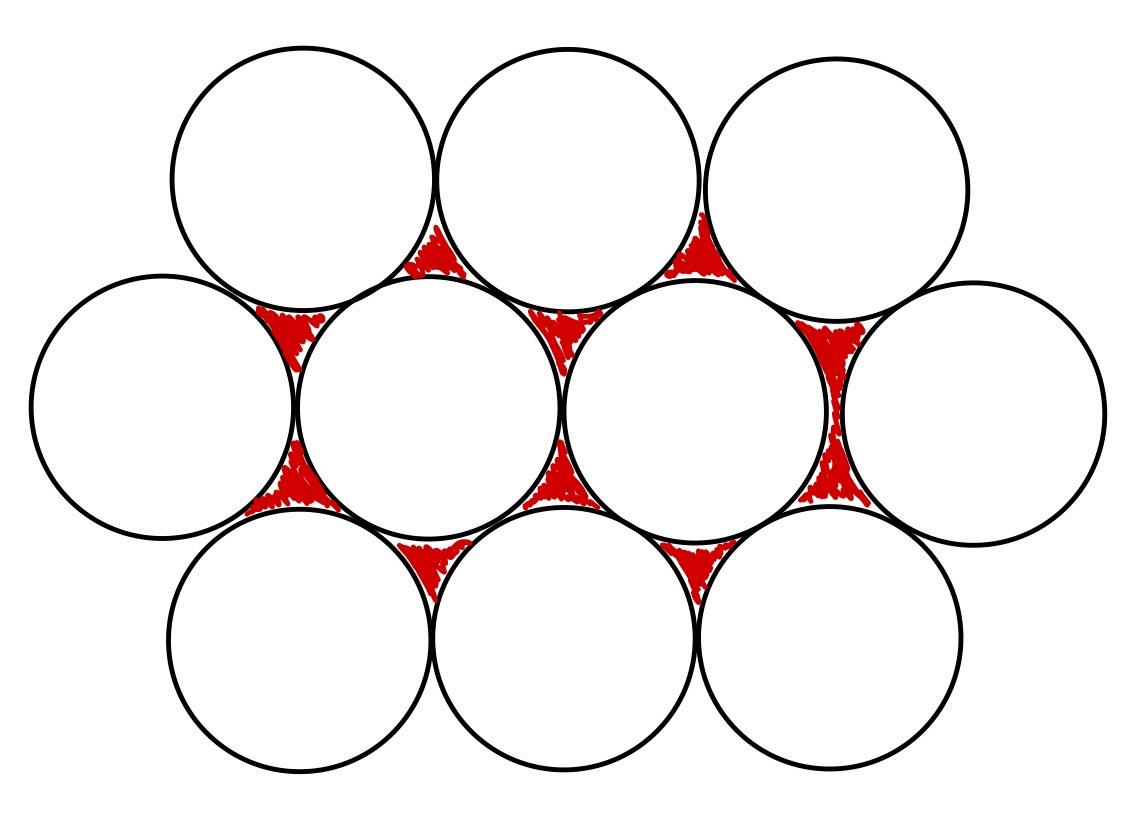
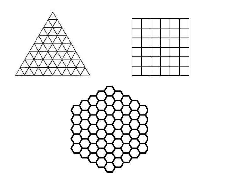
When multiple circles gather to form a honeycomb, empty spaces between each circle are created as well, shown by red colours on the figure above Thus, a waste of space leads to inefficiency in storage. The same applies to most polygons, according to the honeycomb conjecture
However, triangles, squares, and hexagons are exceptional: they are the only polymers that can be clustered without any empty space between them
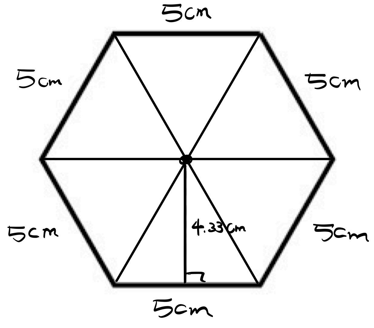
Given the fixed length of 30 cm, one hexagon can produce an area of approximately . 65 0 �� 2 . 5 · 4. 33 · 1/2 · 6 ≃ 65. 0 �� 2
Compared to the area of an equilateral triangle (43.3 cm2) and the area of a square (56.3 cm2), a hexagon (65 0 cm2), can produce the greatest possible area
Ultimately, in the context of honeybees, the use of hexagons allows them to maximize the area for honey storage while simultaneously minimizing the use of materials to build their honeycomb.
4 Conclusion
The honeycomb conjecture is crucial to bees, as it takes a lot of energy for them to produce even a small amount of beeswax To make 1 ounce of wax, bees must consume approximately 8 ounces of honey The efficiency of hexagon tiling is indeed a fascinating principle that can connect to various applications such as computer science, engineering, or even construction, greatly enhancing our lifestyle and technology
A Geometric Visualisation of the Sum and Product Rules
Elias Brixen 70255@jisedu or id
Pure Mathematics
Key Concept: Differentiation
1 Introduction
If you’ve ever taken an IB or AP mathematics course, chances are that you’ll be familiar with the concept of a derivative. For those new to calculus, the derivative of a function at a point tells you how sensitive the output value is to a tiny
2 Graphical Representation of Derivatives
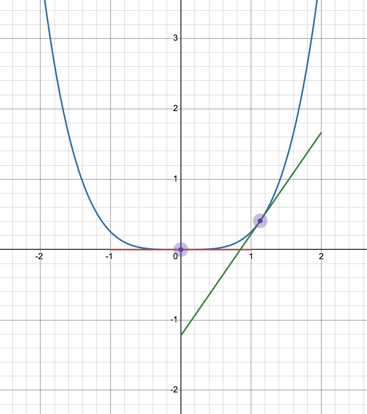
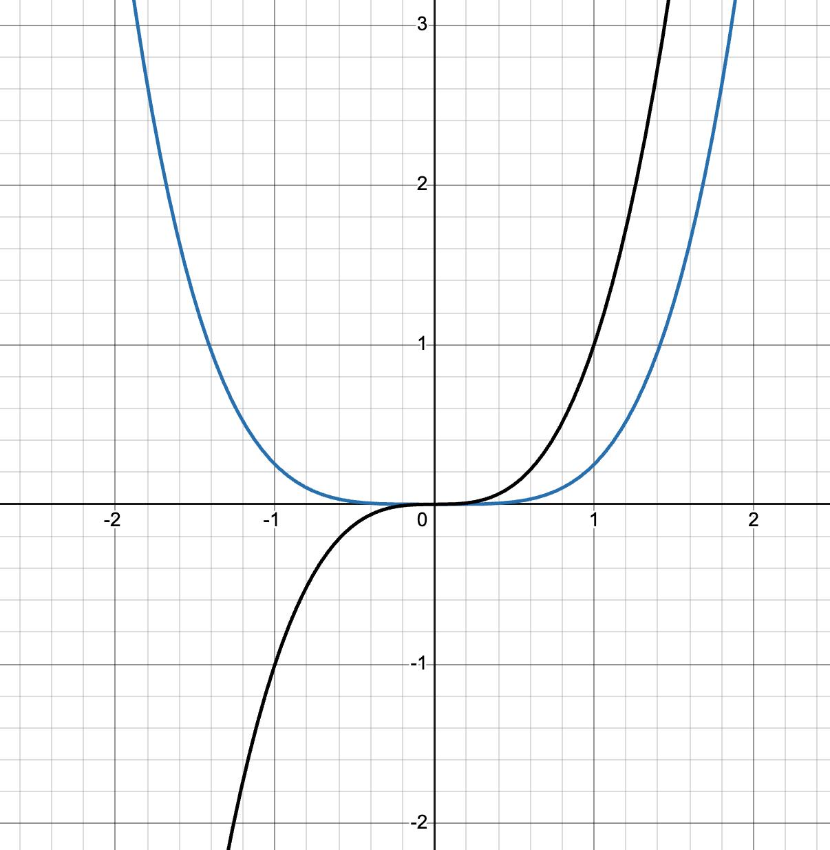
The derivative tells us how sensitive a function is to a change in a tiny increase of the x value at any given point, and are represented by the gradients (slopes) of the tangents to any points along the blue function (the red and green lines). If we collect the sensitivity every single point along the original function, we end up with a graph of the derivative, and tells us how
sensitive a point to change for any input value, as seen below (black line):
3 How can we prove derivative rules?
While this was a graphical representation of the derivative, we are also able to find derivatives analytically through calculus. The task of finding a derivative is often a difficult concept to grasp for many calculus students. There are often arbitrary rules that we students are just taught, with no clear explanation as to why they work. Why does taking the derivative of the sum of two functions mean taking each of their derivatives separately? Why is this different than when two functions multiply with each other?
Often, when we are taught the analytic proof using first principles, the only thing
it really achieves is showing us that the rules work, not really understanding their derivations or how they come to be. There is, instead, a more intuitive way that we can understand where these seemingly nonsensical rules come from.
It’s something that takes us back to the roots of mathematics itself: geometry. To take a step back from all the complicated maths, and explaning the rules through a geometric perspective not only helps us understand the “why” better but can also reveals the underlying beauty of calculus.
There are really only three ways for functions to be made more complex. They can be summed (added together, as subtraction is the same as negative addition), multiplied (division is the same as multiplication by the reciprocal) and composed (have one function inside the other). Each of these operations have rules when it comes to the derivative: the sum, product and chain rule respectively
Understanding them one by one lets us break down any function into its component parts and allows us to take the derivative of nearly every single function thrown at us. Let’s tackle the first two rules step by step (we’ll save the chain rule for another time as it’s a bit more difficult to visualise).
4 Geometric visualisation of the sum rule
Suppose we have a function h(x) that is defined as the sum of two other functions of x, call them a(x) and b(x). In other words, f(x)=a(x) + b (x)+... as many times as we like, and so on.
Let’s say our function is �(�) = � 2 + 4� + 3
The sum rule tells us that find the derivative of f(x), we just take the derivative of each function individually. In other words and so �'(�) = �'(�) + �'(�) + �'(�) on, until we’ve taken the derivative of every term. Why does this work?
It’s useful to think of each “mini” function that makes up f(x) as a geometric shape, with the area representing its total value. Remembering that the area of a rectangle is base height, we can think of f(x) as the × sum of three rectangles like so:
Okay, so how does this help us? From now on, I’ll be referring to the derivative of the function f as Why this notation? It is a �� �� more useful representation of what the derivative is: the amount of a tiny change in the overall function to a tiny change in � the input . In other words, by how much � does the function change as we increase x by a tiny value? Let’s put this into practice. We are going to increase the value of x by a minuscule amount, call it dx. What happens to our original function?
As we can see, we extend the function wherever x is by an arbitrary amount, which we call dx. We add this tiny value of (call it dx) to any x value, essentially extending the sides that have length “x”. Notice how the last constant term doesn’t get an increase of dx? This is because there is no value of x that we can extend; changing the x value doesn’t affect how much the constant term adds to the area of the original function, as it will always be a constant amount, which is also known as the constant rule. The derivative of a constant, or the amount of area that it adds to the original function as we change the input value, is zero.
What about the other two terms?
Remember, we are asking how much the total area of changes df as we add dx. So � let’s take a look! As we can see, we’ve extended any side of length x by this tiny value dx. Let’s calculate the area of the smaller rectangles that we’ve created, that include this length dx (the yellow section).
As the area of a rectangle is its base times its height, we see that we have two pieces of length (from the area x2), one of � · �� length (from the area 4x), and a 4 · �� square with area (the orange bit). �� · ��
Writing this down as an equation, we get this: the change in the total area of the original function as we increase x by a tiny amount:
�� = ��� + ��� + 4�� + ����
As dx gets closer and closer to zero, however, we’ll notice that the amount of area added by becomes negligible. ���� Let’s collect like terms and simplify the expression, so we get:
�� = 2��� + 4��
Finally, let’s divide by dx to get ratio of the change in area as a result of a change in x, and we get: �� �� = 2� + 4
�'(�) = 2� + 4
And we now have a function to compute the derivative at any point!
Notice how in the beginning, each term was independent of each other?
The change in the total area of the function is just the change in the area of all the � functions independently! And so we have the sum rule.
5 Geometric visualisation of the product rule
Let’s now try to derive the product rule, which states that if we have a function h(x) that is defined by the multiplication of two other functions, say f(x) and g(x) then the derivative of h(x) is like so:
ℎ(�) = �(�) · �(�)
ℎ'(�) = �(�)�'(�) + �'(�)�(�)
Why is it different than the sum rule? Let’s visualise this. It’s useful to think of the product of two numbers as a rectangle, with the area representing h(x). For this example, let f(x) be x2 and g(x) be sin(x).
So now,
ℎ(�) = � 2 · ���(�)
Knowing that area = base height, we can · visualize the rectangle like so:
Now, how do we take the derivative of this? Let’s increase the value of x by a tiny amount, and see what happens to the overall area of the rectangle.
derivative of h(x). So what changed? It’s the sum of the two yellow rectangles plus the sum of the orange square.
We see, though, that as our increase in the change of x gets closer and closer to zero, the area added by the orange square becomes negligible (it basically becomes zero times itself) compared to the value added by the other yellow rectangles. So
ℎ'(�) = � 2 · �(���(�)) + ���(�) · �(�2)
And remember that that “d” is just the function’s sensitivity to incremental changes in x, or in other words, its derivative. So we compute and substitute, yielding:
We notice something interesting. Why are the tiny values (d(x2) and d(sin(x))) that we increase x not the same? Think about it this way: each function has a particular “sensitivity”, or how fast they react to changes in x. The sensitivity for our functions above, x2 and sin(x) are naturally different, as they are unique functions. Therefore, when we consider what happens when we increase the value of x by a tiny amount, we treat each function’s change separately.
That’s why we see in the diagram that the side length of x2 increases by its function’s sensitivity (d(x2)) and the side length of sin(x) by its own sensitivity sin(x2).
To finish it all off, let’s consider what effect this has had on the total area of h(x). Remember, the area that we added to the overall rectangle by increasing the side lengths by a tiny amount of x (considering each function’s sensitivity) is the
ℎ'(�) = � 2 ���(�) + ���(�) 2�
Which, if we take a closer look, actually has the same form as this:
ℎ'(�) = �(�)�'(�) + �'(�)�(�)
And there we have the product rule!
6 Conclusion
And that’s a visualisation of two fundamental rules of calculus. By no means are these visualisations exhaustive proofs, nor should they be attempted to be seen as such. They are ways that almost anyone can grasp basic ideas of calculus without much complex background knowledge needed. They showcase an underlying beauty behind the intricate mathematics, revealing simple origins behind what initially seems like a tangled web of complexion.
The Intricate Exploration of the Mandelbrot Set
Jihoo Lee
70598@jisedu or id
Pure Mathematics
Key Concept: Mandelbrot Set
1 Introduction
When zooming in on the delicate, crystalline facets of the snowflakes, they reveal intricate, repeating patterns that often display striking six-sided symmetry. This self-replicating hexagonal structure relates to the striking mathematical object called ‘The Mandelbrot Set’. Based on the mathematical area of ‘Hyperbolic geometry,’ which describes the properties of surfaces with negative curvature, the study of this set demonstrates how simple mathematical rules can generate astonishingly complex and beautiful fractal patterns. Now, let us explore this set more thoroughly.
2 Background Information
The Mandelbrot Set was created by Polish-born mathematician Benoit B. Mandelbrot, also known as “the father of fractals.” From 1979 to 1980, he discovered the Mandelbrot set by utilizing computers, exploring complex mathematical equations, and iterating a simple function on the complex, especially for the simple equation �(�) = � 2 + � using the Fibonacci sequence. The terms z and c are complex numbers consisting of imaginary and real numbers.
3 Structure and Application
The Mandelbrot set features a basic cardioid shape - the central heart-shaped region- consisting of numerous ‘bulbs’. Each bulb is a large disk directly attached to the cardioid, together with numerous other smaller bulbs and a prominent ‘antenna’, which refers to the thin, spiky structures that extend outward from the cardioid.
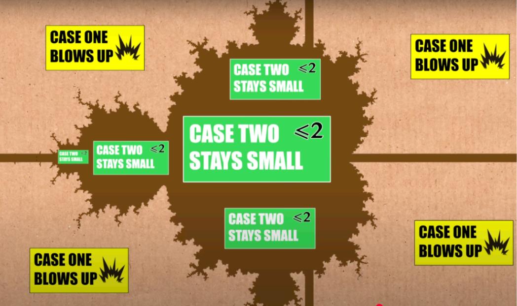
Here, the set presents two cases: Firstly, if the orbit fails to go to infinity, it is � � � 0 bounded in the Mandelbrot set. Secondly, if the orbit reaches infinity, the point � � � 0 is outside the set.
�(�) = � 2 + �
� 0 = 0
After iterating the value, then
� 1 = 02 + � = �
� 2 = � 2 + �
� 3 = (�2 + �)2 + �
� 4 = ((�2 + �)2 + �)2 + �
* The constant C is a value that can be altered.
As seen from the equations above, the output of Z becomes greater. Some values of c, when plugged into this iterative function, produce outputs that swiftly soar toward infinity. The points outside the set grow exponentially in a fast manner when they are put through the equation many times in the function.
The equation can be �(�) = � 2 + � altered to represent another function to obtain a sequence of � �+1 = � � 2 + � 0 complex numbers . � � � = 0, 1, 2,...
1 = � 2 + � = 1 + �
2 = ( 1 + �)2 + � = 2� + � = �
3 = ( �)2 + � = 1 + �
4 = ( 1 + �)2 + � = �
In this case, further iterations will repeat the values , which fail to reach 1 + � infinity and become bounded in the set.
(Figure 1. Types of cases observed on the Mandelbrot Fractal)
It is important to remember that the points inside the Mandelbrot Set have to be within the boundary limit of 2. With both
equations, when a new point is run, the values revert to their original amount.
4 Appearance of the Mandelbrot Set
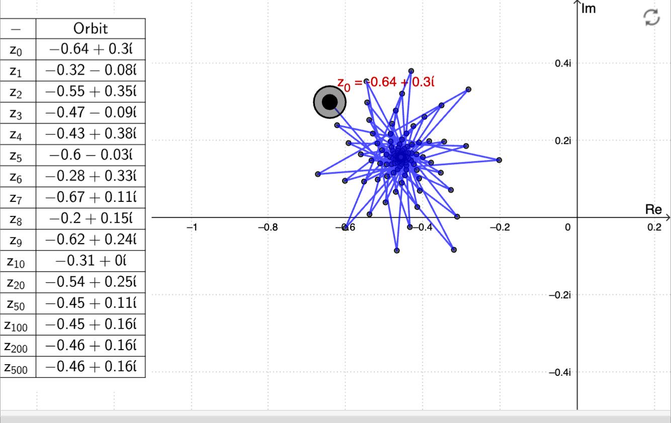
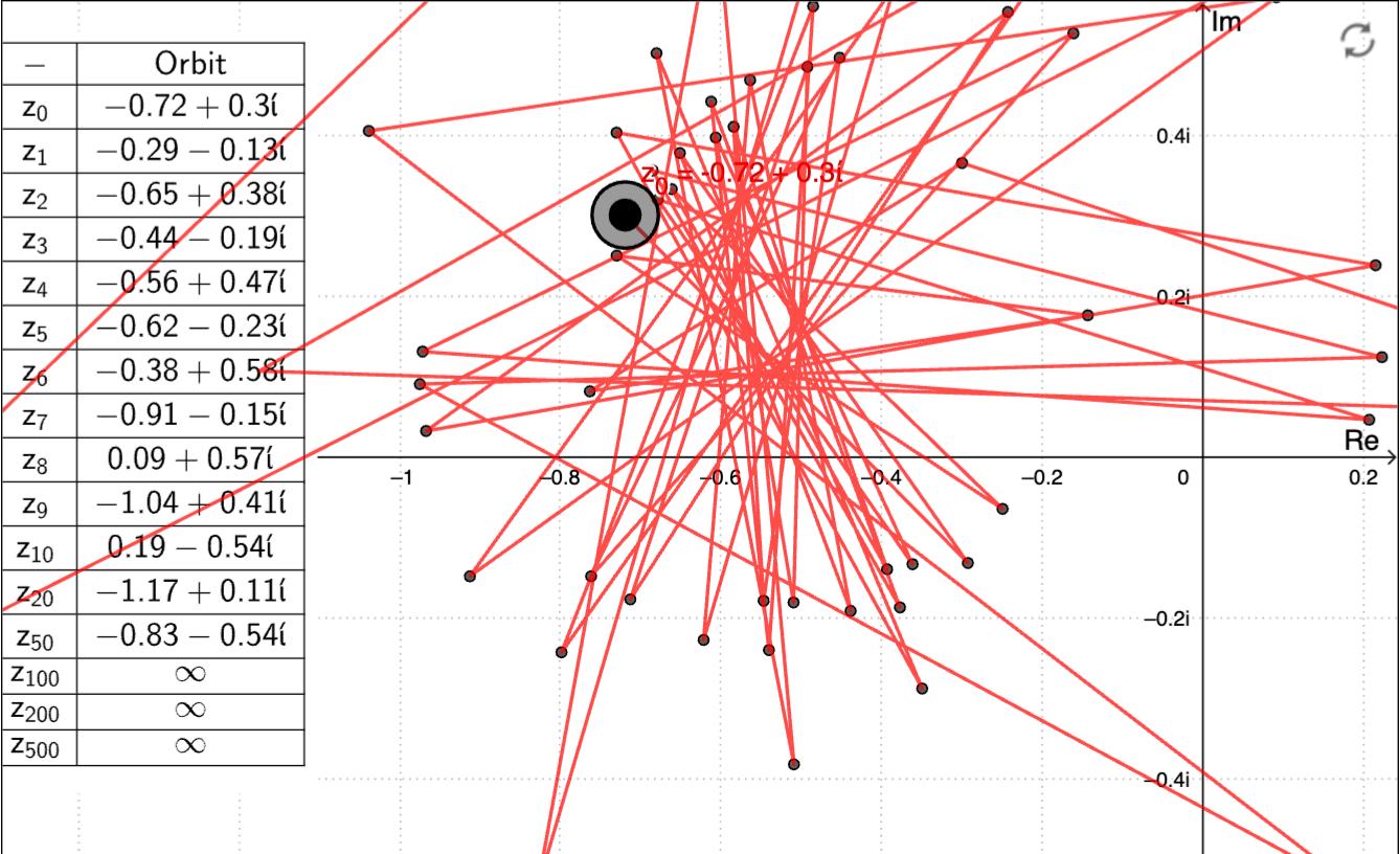
Visualizing an endlessly complicated Mandelbrot set, its behavior can be shown with a complex plane by plotting the values.
(Figure 2. Shape of the Mandelbrot set with an equation of � 0 = 0. 3� 0. 64 plotted on Geogebra)
(Figure 3. Shape of the Mandelbrot set with an equation of � 0 = 0. 3� 0. 72 plotted on Geogebra)
If the constant C from the equation changes, the graph forms an unpredictable pattern like spiral shapes, determining whether the orbits are fixed or behave ‘chaotically’.
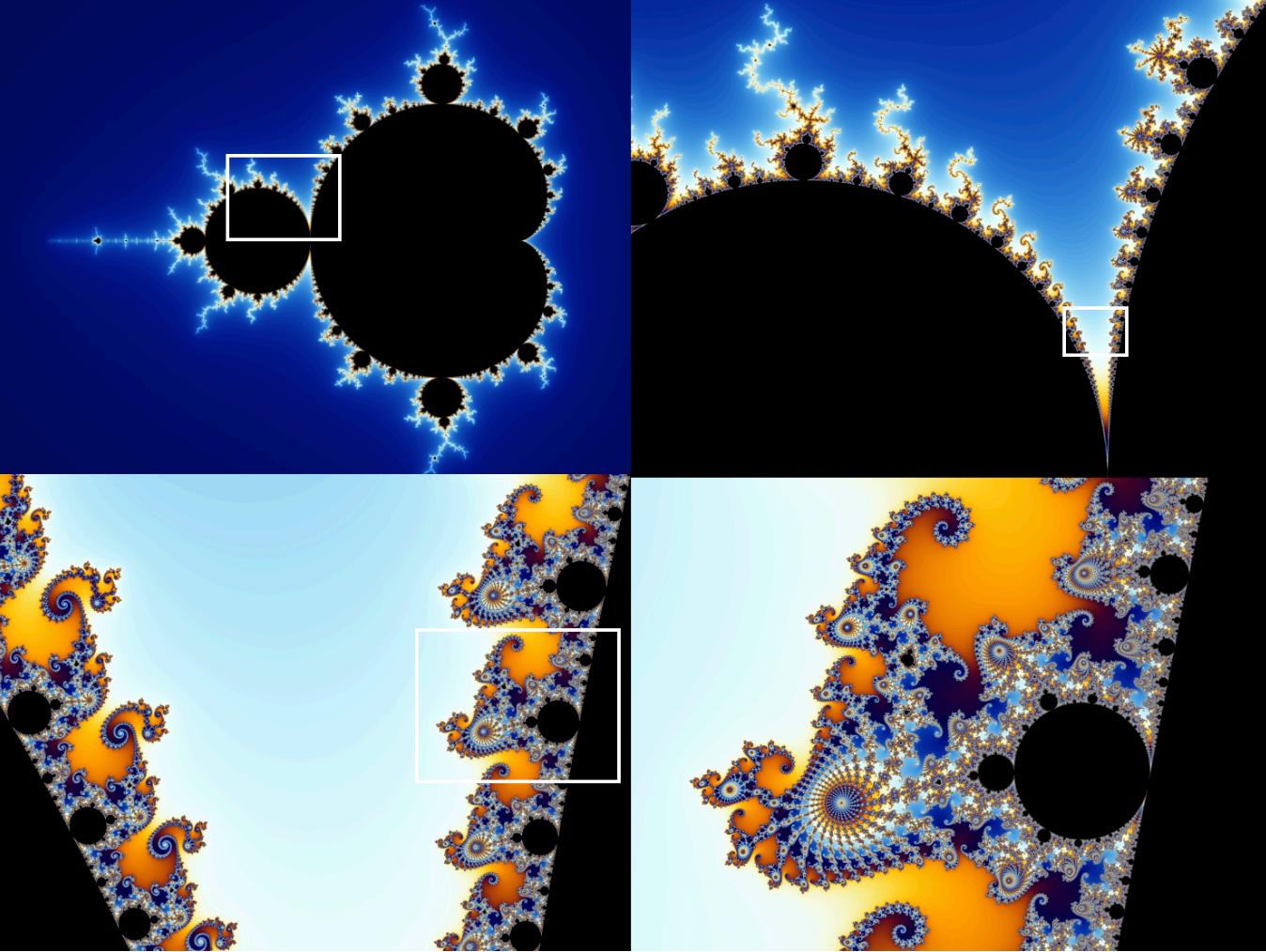
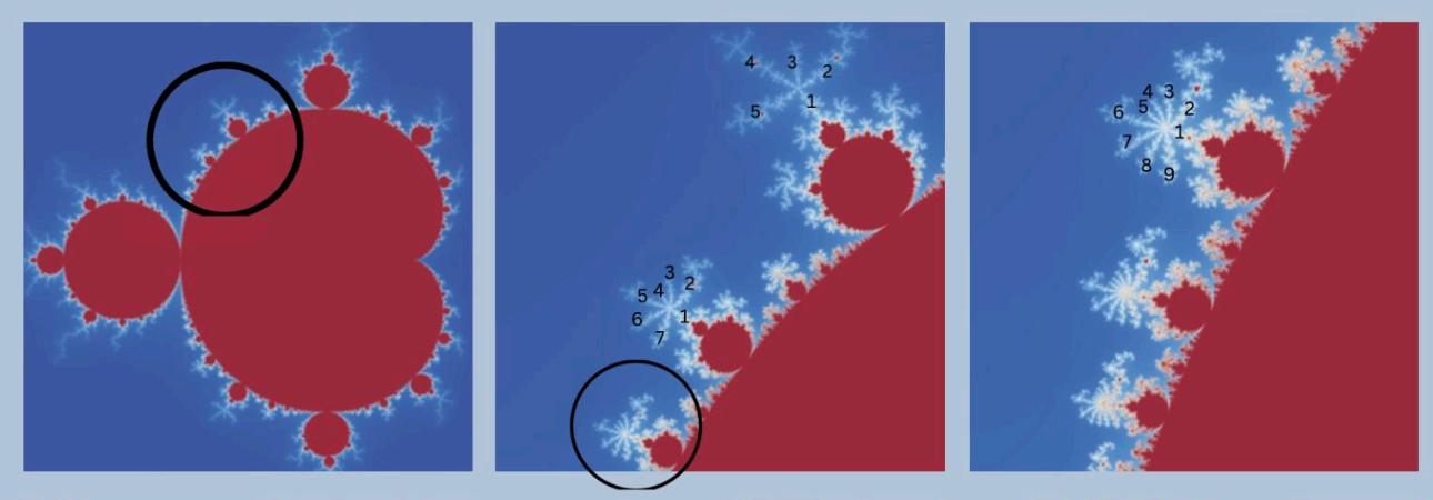
(Figure 4. Zoomed-in diagram of the Mandelbrot Fractal)
Furthermore, infinitely complicated repeating patterns can be seen when zooming in on the set's boundary. Since the patterns tend to be exact replicas of each other and reoccur on a smaller scale, it pictures a ‘Seahorse Valley’ centered around . 0 1� 0 75
As mentioned, the equation of the Mandelbrot set is based on the Fibonacci sequence. For a disc attached to the main cardioid, the cycle number can be known from the number of branches in the antenna associated with the disc. As shown from the diagram below, each bulb increases in branches by 5,7,9,11,13,... .
(Figure 5. The Complex Border Behaviors of the Mandelbrot Set)
Moreover, the fractal formula of the spiral fractal obtains the formula , � = � τΘ where r is the radius of the spiral, is the τ growth rate, and is the angular Θ coordinate. The equation , � = � τΘ related to the Fibonacci sequence, describes an exponential growth of the radius as it increases. If > 0, the spiral Θ τ expands outward. And if < 0, the spiral τ contracts inward. This equation allows us to analyze the rotation and tightness of Mandelbrot spirals and predict the behavior of the spiral arms at deeper levels.
5
Conclusion
Hence, the Mandelbrot Set demonstrates the border between stable and unstable, which makes it renowned for its infinite complexity. This complexity comes from its fractal nature, where infinite detail can be identified at any magnification level. Mathematically, due to its nonlinear iteration, the Mandelbrot set exemplifies how simple mathematical rules generate incredibly complex and beautiful fractal patterns.
Section 2: Applied Mathematics
1. Analyzing Probability Theory in Corporate Risk Management - Keiko Kaliman
2. Application of Mathematics in Medical Imaging - Dowon Her
3. Where Will Crimes Occur: An Introduction to Kernel Density Estimation - Chaeyeoung (Amy) Lee
4. Analyzing Probability Theory in Corporate Risk Management - Chaewon (Wendy) Yang
5. Application of Statistical Analysis in Sports: The Effect of Launch Angle and Exit Velocity on the Success Rate of Home Runs - Jinwoo Yang
6. Binary and Hexadecimal Math in MicrocontrollersVincent Tjoa
Analyzing Probability Theory in Corporate Risk Management
Keiko Kaliman 69759@jisedu.or.id
Applied Mathematics
Field of Application: Natural Science
1 Introduction to the Lab Scientist’s Dilemma
Dr. Wilmena stood in her company’s top research facility, staring at the rows of test tubes before her. She had just received a disturbing threat: one of the 500 vials in her laboratory had been tampered with and replaced with undetectable poison. If injected into one of her test subjects– an extinct species of animal– it would cause a lethal mutation and eradicate the species forevermore. She only had an hour until all the vials were administered to their respective subjects, and Dr. Wilmena needed to act before it was too late.
Unfortunately, there was only enough time for her to do one trial. Fortunately, she could test multiple trials at the same time. She had to test it on her precious lab rats, but being an animal lover, she wanted to minimize the number of lab rats she had to test on.
Thankfully, she had a great idea she could implement, using the binary system she learned recently from the great German mathematician Gottfried Wilhelm Leibniz. Let me share her idea with you.
2 The Denary System
Before introducing the binary system, let me introduce the denary system– the system we mainly use to count. It is a base ten system, with each digit being one of the integers from 0-9. The value of the digit in the nth place is the digit itself multiplied by 10� 1
For example: 7014: 7 ×
3
The Binary System
Now, let’s get on to the binary system. Unlike the denary system, the binary system is counted in base 2, which means that only 0 or 1 can be used for each unit place. The value of the nth place is equal to the digit multiplied by 2n-1 .
For example: 1011:
1 × 23 + 0 × 22 + 1 × 21 + 1 × 20
8 + 0 + 2 + 1 = 11
As you can see from the example above, the Binary System can be converted to the Denary System.
While it is generally used for computer programming, it can also be utilized to solve real-life problems like the one introduced above. Now that I’ve introduced the system, let’s get back to Dr. Wilmena’s story
5 Dr. Wilmena’s Plan
With the help of Binary Counting, she was able to create more than 500 combinations just with 9 lab rats, minimizing the number of animals she had to test on. This is because 29 = 512, which is more than enough binary codes she needs. She labeled the vials from 0 to 499.
She turned the labels into a binary expression, which is at most 9 digits long, representing which lab rats the vials will be injected into. If the state of the rat matches the configuration of the binary expression, 1 for dead and 0 for alive, it would mean that she had found the poisoned vial.
Her plan was that for each bottle, the digit 1 in the nth position from the right in the binary configuration means the nth rat from the right, when rats are put in descending order, drinks the bottle of wine.
Let’s say that the 57th bottle of vial was the one poisoned.
Rats 1, 4, 5, and 6 would have been injected with the poisoned vial and died.
Rat 1: 1, 3, 5, …, 55, 57, 59, …
Rat 2: 2-3, 6-7, 10-11, …, 54-55, 58-59, …
Rat 3: 4-7, 12-15, 20-23, …, 52-55, 60-63…
Rat 4: 8-15, 24-31, 40-47, 56-, …
Rat 5: 16-31, 48-63, …
Rat 6: 32-63, …
Rat 7: 64-127, …
Rat 8: 128-255, …
Rat 9: 256-511, …
Rat 10: 512-1000
57
By using just nine lab rats and seconds to spare, Dr. Wilmena was able to save all the extinct species by identifying and removing the poisoned vial. Do you think you could’ve used fewer lab rats in the time constraint?
Application of Mathematics in Medical Imaging
Dowon Her 67817@jisedu or id
Applied Mathematics
Field of Application: Optics
1 Introduction
X-ray technology is the epitome of how physics can be applied in the fields of biomedical sciences The principles of wave properties allow X-rays beamed into the body to reflect, refract, and diffract, providing us with a visual of our skeletal and muscular systems Mathematical modeling plays a crucial role in predicting and analyzing the results of X-ray radiation
2 Mechanism of X-ray test
When X-rays are beamed into our body, the waves interact differently with different parts of the body such as bones, organs, and muscles. For example, when X-rays are incident on a muscle tissue, most of the waves are going to be absorbed by the tissue and only some will be reflected back, which makes organs to appear dark in the radiograph. On the other hand, when X-rays are incident on a bone, most of the waves are reflected, which makes it appear bright in the resulting image. Through mathematical modeling, it is possible to interpret this phenomenon.
3 Attenuation through one material
When X-ray waves encounter a material, they gradually lose their intensity as they travel through the material. This phenomenon is called attenuation. The magnitude of attenuation depends on several factors, including the nature of the material, linear absorption coefficient(μ), and the thickness that the wave travels (x).
This formula represents the exponential decay of the intensity of X-ray as
the distance (thickness) in which it travels increases. The negative exponent of e shows that as the linear absorption coefficient increases, there is a greater decrease in the intensity of X-ray after traveling x distance of the material. The linear absorption coefficient is a constant that shows how well a material can absorb X-rays. For example, materials such as lead have extremely high linear absorption coefficients, which makes it useful in covering vital organs when performing an X-ray test on human beings.
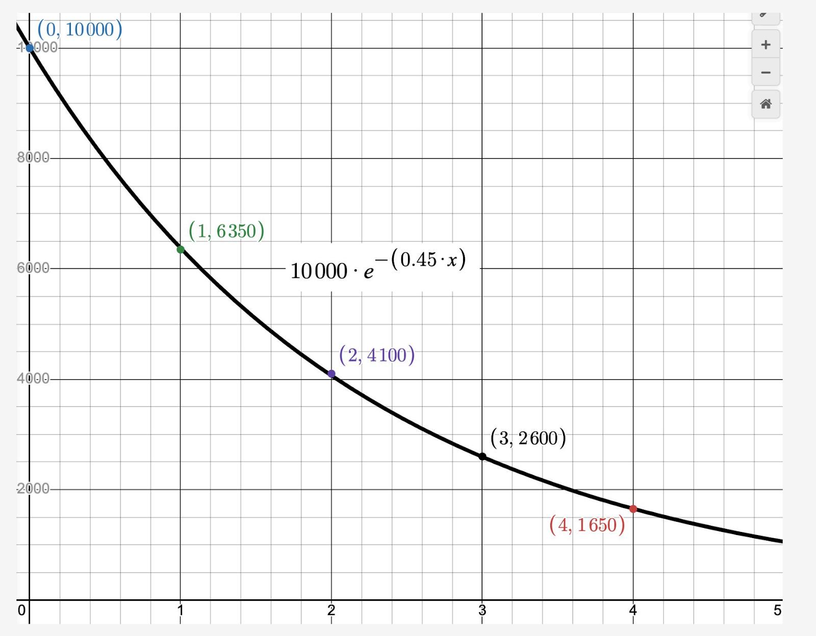
A typical fat in our body has a linear absorption coefficient of 0.45. Lets assume that the intensity of the X-ray incident on the fat is 10,000 photons. Then, depending on how far the X-ray travels through, the intensity of the X-ray will change as the following graph
Here, we can see that as the X-ray travels further into the fat, its intensity decreases exponentially from 10000 to 1650 at the thickness of 4
3 Attenuation through two materials
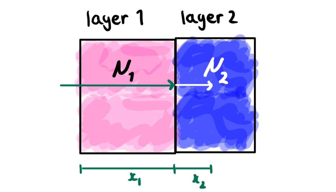
In most cases, X-rays do not travel through only one uniform material but rather
through multiple layers of different materials The same formula can describe the attenuation as the wave travels through two materials
As stated above, when an X-ray passes through a distance x of a material then the resulting intensity left is equal to � = � 0 � µ1�1
. When it travels through a second material, then the new incident intensity of the X-ray will be In other words, that is the � 0 � µ1�1 intensity at the moment when the wave starts to travel through the second material.
Using the same reasoning, � µ2�2 should be multiplied to where μ2 is the � 0 � µ1�1 linear absorption coefficient of the second material and x2 is the distance in which the wave travels through the second material Using the rules of multiplication of exponents with the same bases, the resulting expression for the final intensity of the X-ray is
� 0 �
(µ1�1+µ2�2)
Similarly, if the X-ray travels through 3, 4, 5, 6, and n different materials, the expression of the final intensity will be
� 0 �
(µ1�1+µ2�2+µ3�3)
(µ1�1+µ2�2+µ3�3+µ4�4)
� 0 �
� 0 �
(µ1�1+µ2�2+µ3�3+µ4�4+µ5�5)
(µ1�1+µ2�2+µ3�3+µ4�4+µ5�5+µ6�6)
� 0 �
� 0 �
(µ1�1+µ2�2+µ3�3+µ4�4+µ5�5+µ6�6+ + µ���)
properties of mathematics allow us to simplify complex phenomena in real life Organs with high attenuation will therefore appear darker and bones that cause low attenuation will appear brighter
4 Attenuation and impedance in ultrasound imagery
In some cases, such as taking an image of a fetus in a pregnant woman, it can be dangerous to use X-ray imagery This is because X-ray is the wave with the second highest energy after gamma rays In these cases, we can use ultrasound imagery
Similar to X-rays, ultrasound can be absorbed, scattered, and reflected by different parts of the body, resulting in attenuation Therefore, the same formula applies to the intensity of ultrasound Instead of intensity, we use loudness to express the intensity of ultrasound
� = � 0 � (µ1�1+µ2�2+ + µ���)
There is one more mathematical model for ultrasound imaging, which can predict the quality of the image produced. The quality of the image produced is called impedance, and it depends on two factors, the density of the medium (ρ) and the speed of sound in the specific medium (c).
� = ρ�
This is because as the material in which the ultrasound is traveling becomes denser, it is easier for the sound to be reflected compared to when the sound wave is incident on a non-dense material The easier sound waves are reflected, the clearer the image will be
This demonstrates how basic
Another factor is the speed of sound Sound has different speeds depending on the medium in which it is traveling Sound tends to travel faster in denser objects For example, the density of bone is 1900kg m-3, and the speed of sound is 4100 ms-1 On the other hand, muscle has a density of 1080kg m-3, and the speed of sound is 1600 ms-1 Similar to X-ray imaging, this makes the bones of the body appear clearer than fluids
5 Conclusion
In conclusion, mathematical modeling is extremely helpful in analyzing and predicting the results of medical imaging The mathematical principles behind X-ray and ultrasound imaging are an example of how mathematics can facilitate the development of life-saving technologies
Where Will Crimes Occur: An Introduction to Kernel Density Estimation
Chaeyeong (Amy) Lee 71473@jisedu or id
Applied Mathematics
Field of Application: Criminology
1. Introduction
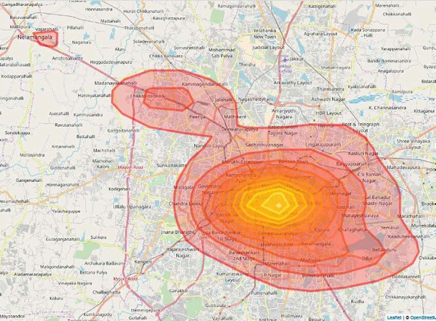
Have you ever seen a map with a colored diagram like the picture below?
The picture above is a hotspot visualization of the crime rate in Bangalore. An area with a color closer to yellow has a higher chance of crime occurrence, and the further away from the point with the highest crime rate, the lower crime rate there is. This analysis of data is critical in identifying the crime hotspot that needs more support in preventing crime
Indonesia in 2022, for example, had a crime rate of 137 per 100,000 population However, this doesn’t mean that all locations of the 100,000 population have the same probability of crime exposure. Mapping out the density probability clearly shows which area is more vulnerable to crime and facilitates efficient execution of law and distribution of funds and police force.
To draw this map, first, data about the specific location of crime should be collected. After a sufficient data set is gained, graphing is done using GIS software or programming tools In the process of visualizing data, math in statistics is used: kernel density estimation. Kernel density estimation is a concept that applies kernel smoothing to graph the probability density It is a non-parametric method – involves minimum assumptions for a hypothesis such as normal distribution – to analyze the relationship between a random variable and its probability
2. Kernel Function
The Kernel function should be understood first before diving into the Kernel density estimation The kernel function K(x) generally measures the similarity or transformation between data points, and it is identified by three key features
Statistics, in particular, estimate how each data point influences the probability density at a given location using the kernel function. There are multiple types of Kernel functions; the most commonly applied one for Kernel density estimation:
The equation above is the standardized form for the Gaussian kernel regression, and d indicates the dimension This function assumes that the data follows a standard normal distribution (mean = 0, standard deviation = 1). For example, in a given data set of x = [-2,-1,0,1,2] in one-dimensional, the Gaussian Kernel values are:
K(-2) = 0.05399
K(-1) = 0 24197
K(0) = 0 39894
K(1) = 0.24197
K(2) = 0 05399
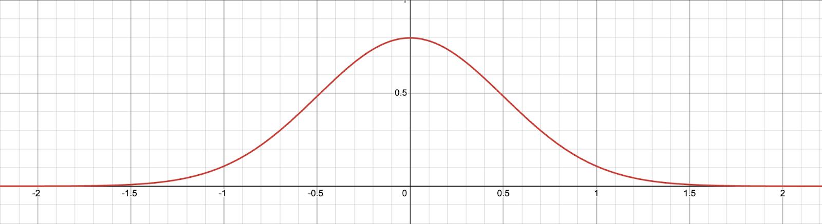
Here, the maximum point is at x = 0, and it is symmetric around x = 0 because K(x) = K(-x). The plotted graph looks like below: a bell-shaped curve
Although not necessary, some Gaussian kernels have standard deviations( ). This acts σ as a scaling factor that controls the spread of the data points. The Gaussian kernel, including standard deviation in one dimension, will look like this:
If this equation is used to graph the same data set but with a standard deviation of 0.5, the graph will be different from the original one.
K(-2) = 0 00027
K(-1) = 0.10798
K(0) = 0.79788
K(1) = 0 10798
K(2) = 0 00027
The graph will look like below
Graph #2 is narrower than Graph #2 due to a smaller standard deviation This means that for the same horizontal change, the vertical change is greater. Therefore, a larger standard deviation smoothes the graph, and a smaller one makes the function more sensitive to changes in the x value
3. Kernel Density Estimation
In kernel density estimation, standard deviation is replaced with bandwidth (h) – a real positive number that defines the smoothness of the function. The equation for Gaussian Kernel and Kernel density estimation looks like this:
The reason why there is a standard deviation divided in the function is because the integral of the graph should be kept 1
In one dimension, where d=1, the equation looks like this:
variable meaning
�(�)
Estimated density function at x
� Total number of data points in the data set given
ℎ Bandwidth parameter
d Dimension
� The location to estimate density (query point)
� � A data point from the data set given
� � � Relative distance from each data points
Let’s look at an example where the x = 0 5
The data set is the same x = [-2,-1,0,1,2], and a standard deviation of 0.5 from previous examples
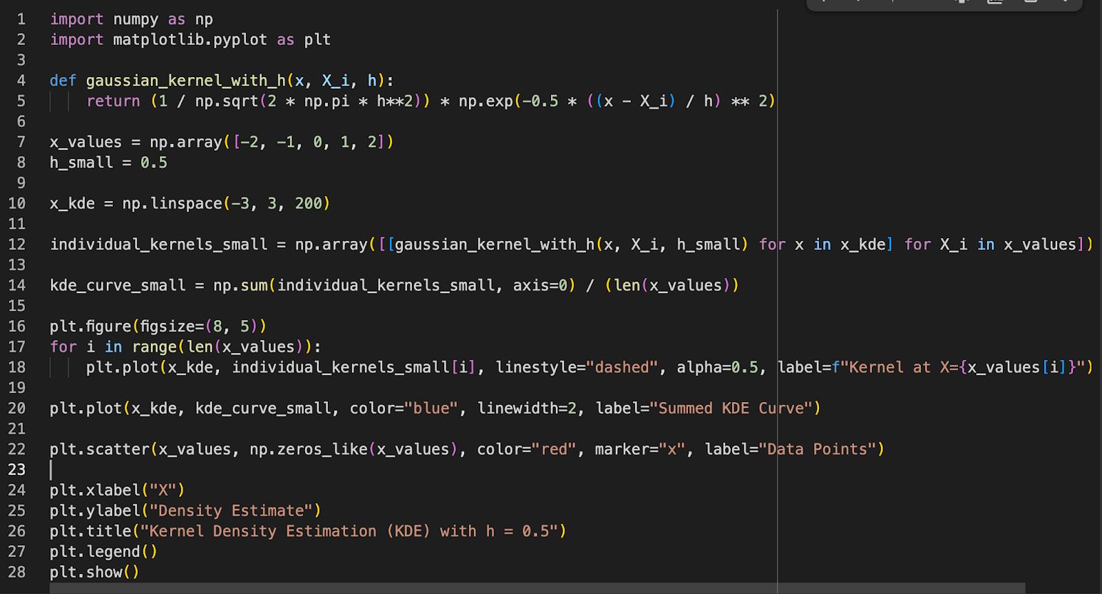
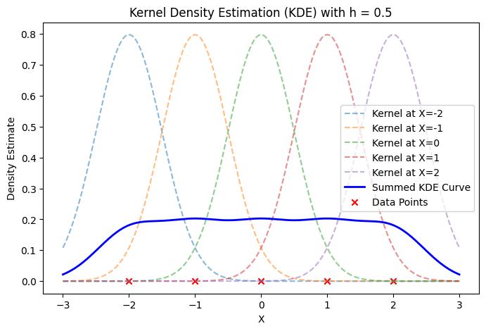
This means in the density probability graph, at x = 0.5, the output will be 0.197123. The same process is followed to calculate the kernel density estimation value for all random x values These points can be plotted on the coordinate plane by using coding.
4. Kernel Density Estimation in 2-D
Kernel Density Estimation can be used in various dimensions, not just one dimension In two dimensions, a different Gaussian kernel function is used.
ℎ(�, �) = 1 2πℎ2 � ( � 2 +� 2 2ℎ2 )
= 1 � �=1 � ∑ 1 2πℎ2 � ( (� ��)2+(� ��)2 2ℎ2 )
For example, let’s say three crime cases occurred at points (1, 1.5), (2, 2.5), (3, 3.5), and the bandwidth is 0.5. If we are looking for the kernel density estimation value at (2 5,1)
When ( ) = (1, 1.5) � � , ��
�ℎ(2 5, 1) = 0 00429
When ( ) = (2, 2 5) � � , ��
�ℎ(2. 5, 1) = 0. 00429
When ( ) = (3, 3.5) � � , ��
�ℎ(2. 5, 1) = 0. 0000007
�(2 5, 1) = 1 3 (0 00429 + 0 00429 + 0 0000007)
= 0 00286
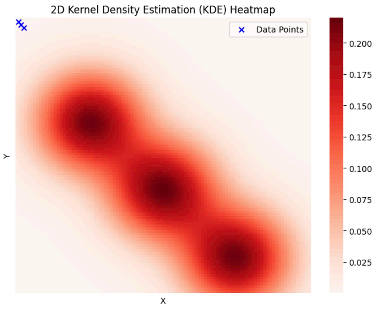
This means that in the density probability graph, at (2 5,1), the output will be 0 00286 Using the same process for other points, the data can be plotted as a heatmap, which can be done by programming.
In this graph, the darker the red, the higher the density probability The three dark red spots correspond to the three given data points (1,1 5), (2,2 5), (3,3 5) As the points get farther from the three points, the color becomes lighter.
5. Evaluation of Limitations
Although it is beneficial to visualize crime data with Gaussian kernel density estimation, it has some limitations First, it is difficult to find the optimal bandwidth: over-smoothing may miss out important data patterns, and under-smoothing may lead to excessive hot spots The Kernel function follows the normal distribution, so the data points at the edge aren’t highly accurate (edge effect) Especially, density at the boundaries tends to be underestimated, which results in biased data Also, in Kernel density estimation, all events are treated with equal weight However, not all crimes have the same severity and recency, and some crimes may happen over the course of time rather than temporarily.
6. Conclusion
In this article, we explored how Kernel density estimation is applied to crime data analysis It is a very useful technique that helps to identify crime patterns and provides valuable insight into policymaking and urban planning Although there are limitations in bandwidth, edge effect, and static analysis, Kernel density estimation can be integrated with other methods to alleviate them Researchers continue to explore it and apply it to not only criminology but various areas that require density probability analysis.
Analyzing Probability Theory in Corporate Risk Management
Chaewon(Wendy) Yang 71446@jisedu.or.id
Applied Mathematics Field of Application: Business
1. Introduction to Probability in Business
Mr. Reynolds, a risk manager at a big investment company, sat at his desk reviewing two possible projects. Both projects could make a lot of money, but they also came with serious risks. One project involved investing in a new tech startup that promised fast growth but had no proven track record. The other involved investing in a more stable company that had steady profits but offered lower returns. With millions of dollars involved, Mr. Reynolds could not just guess which project was the better choice.
This is where probability theory becomes useful. Probability theory is a branch of math that helps people figure out how likely certain events are to happen.
In business, it is used to predict potential risks and rewards, which is exactly what Mr. Reynolds needed. By using probability, he could calculate the chances of success and failure for each project and understand the possible financial results. This gave him a clearer idea of what might happen and helped him avoid making decisions based only on guesses or hope.
2. Understanding Probability
Before we dive into business applications, let’s cover the basics of probability theory.
Probability of an Event (P)
Probability measures how likely an event is to occur. It ranges from 0 (impossible) to 1 (certain): 0 ≤ �(�) ≤ 1
For example, the chance of flipping a coin and getting heads is: �(�����) = 1/2 = 0. 5
3. Expected Value: Predicting Averages Over Time
The Expected Value ( ) helps predict the �� average outcome over multiple trials. It’s crucial in business for estimating profits and losses.
The formula is: �� = ∑(�� × ��)
Where:
Probability of outcome �
Value (payoff) of outcome �
Example: Suppose an investment has a 70% chance of earning $10,000 and a 30%
chance of losing $5,000:
�� = (0 7 × 10, 000) + (0 3 × 5, 000
This means, on average, the investment yields $5,500 over time.
4. Measuring Risk:
While tells us the average outcome, it �� doesn’t show risk. That’s where Variance and Standard Deviation come in.
- Variance( : Measures how far ���) outcomes spread from the expected value. ���(�) = ∑(�� × (�� ��)2)
- Standard Deviation( ): Gives the �� spread in the same units as the data. ��(�) = ���(�))
A higher means more risk, while a �� lower suggests more stable outcomes. ��
5. Comparing Risk and Reward: Coefficient of Variation
Businesses often compare investments using the Coefficient of Variation ( ),�� which shows risk relative to expected return. �� = ��/��
- A lower = better risk-return �� balance
- A higher = higher risk for each �� dollar earned
6. Applying Probability Theory: Mr. Reynolds’ Decision
Project A:
- 60% chance to earn $100,000 - 40% chance to lose $50,000
Project B:
- 50% chance to earn $150,000 - 50% chance to lose $100,000
Mr. Reynolds repeats the process for Project B and finds that Project A not only offers higher returns but also a better risk-reward ratio.
7. Real-World Business Applications
1. Marketing Forecasting: Predicting Stock Prices and Market Trends
Financial markets are unpredictable, but probability models help investors make better decisions. Analysts use historical data and probability distributions to estimate future stock prices and economic conditions.
Example: Using Probability to Predict Stock Prices
Imagine a company’s stock price today is $100. Based on past trends, analyst predict:
- 40% probability that the stock will rise to $120
- 35% probability that it will stay at $100 - 25% probability that it will drop to $80
Using the Expected Value ( ) formula, �� investors estimate the average future stock price:
�� = (0. 4 × 120) + (0. 35 × 100) + (0. 25 × 80
�� = 48 + 35 + 20 = 103
Since the expected stock price is $103, an investor might consider buying the stock, expecting it to grow in value. However, they must also consider risk by calculating variance and standard deviation to see how much the price might fluctuate.
Advance probability models, like the Monte Carlo Simulation, simulate thousands of possible future stock movements, helping investors prepare for different scenarios.
2. Insurance Premiums: Calculating Risk and Setting Prices
Insurance companies rely on probability to calculate how likely a customer is to file a claim. They use this information to set fair prices for insurance policies, ensuring they
make enough profit while covering potential losses.
Example: Setting Car Insurance Prices
An insurance company analyzes accident reports and finds that:
- A young driver (under 25) has a 10% probability of getting into an accident.
- An experienced driver (over 25) has a 2% probability of an accident.
If an accident costs the company an average of $20,000, the company calculates the Expected Payout ( ) for �� each driver:
For a young driver: �� = 0 1 × 20, 000 = 2, 000
For an experienced driver: �� = 0 02 × 20, 000 = 400
Since young drivers have a higher risk, they are charged higher insurance premiums than experienced drivers.
Insurance companies use probability to predict rare events like natural disasters or medical emergencies. This helps them set prices that cover future claims.
3. Project Management: Assessing Business Risks and Returns
Companies use probability to decide whether a new project or investment is worth the risk. Before launching a product, opening a new store, or investing in new technology, businesses analyze potential profits and losses using expected value and variance.
Example: Launching a New Product
A tech company is deciding whether to launch a new smartphone. They estimate: - 60% chance the product succeeds,
earning $5 million - 40% chance it fails, losing $2 million
Using Expected Value, they calculate the potential return:
�� = (0 6 × 5, 000, 000) + (0 4 × 2, 000, 000
�� = 3, 000, 000 800, 000 = 2, 200, 000
Since the Expected PRofit is $2,2 million, the company might decide to launch the product. However, to quantify risk, they also calculate variance and standard deviation. If the risk is too high, they might delay the launch or conduct more market research.
Decision trees and Bayesian probability allow businesses to make smart choices by considering different possible outcomes and updating their decisions as new information becomes available.
8. Conclusion
In the modern business world, probability theory helps companies predict outcomes, reduce risks, and make smarter decisions. It is used in areas like investing, marketing, and insurance to estimate profits and losses. Instead of guessing, companies use tools like expected value and variance to weigh risks and rewards.
With new technology and data analysis, businesses can apply probability more effectively than ever. While no decision is risk-free, understanding probability helps companies make better choices and succeed in an uncertain world.
Application of Statistical Analysis in Sports: The Effect of Launch Angle and Exit Velocity on the Success Rate of Home Runs
Jinwoo Yang
69490@jisedu
or id
Applied Mathematics
Field of application: Sports
1 Introduction
Baseball has developed significantly due to the implementation of advanced scientific statistics in recent years. In the beginning, there were only rough statistics of batting averages and pitching velocities. However, as time passed by, baseball became more sophisticated with involvement of cutting edge technologies.
Two of the most crucial statistics in modern baseball analysis are launch angle and exit velocity. Sports science has found that launch angles and exit velocity are the most accurate in determining the probability of hits becoming home runs. As baseball statistics are becoming more widely used and universal, improving launch angle and exit velocity has become crucial points hitters focus heavily on.
2 Launch Angle and Exit Velocity
Launch angle is the angle of the ball's trajectory after contact. Launch angle determines whether the ball is a ground ball, line drive, fly ball, or pop-up. For example, a negative launch angle means the hit will result in a ground ball while high launch angles mean the ball will become a pop up. Exit velocity, on the
other hand, is a measurement of how fast the ball is traveling off the bat. Combined, these two elements determine the trajectory and distance a ball will travel.
Research from Major League Baseball (MLB) shows that the best launch angle for home runs is between 25 to 35 degrees. This angle allows the ball to fly high and far enough to get over the fence. If the angle is too high, the ball will only go up and not front, while if it is too low, the ball will touch the ground before it even reaches the fence. However, to hit a homerun, you need more than a good launch angle. Exit velocity is equally important. Studies suggest that a hard hit, a hit with an exit velocity of 95 mph or more, significantly increases the probability of a homerun. It should be obvious as the faster the ball travels, the less gravity it will get affected.
In recent years, MLB applied Statcast to all of its baseball games. It measures every pitch and hit in every game, collecting priceless data. After the implementation of Statcast, exit velocity and launch angle values increased significantly. According to Statcast, more than 87% of home runs hit in 2024 had an
exit velocity above 100 mph and a launch angle between 25 and 35 degrees. To look at specific players, in 2022, Aaron Judge hit 62 home runs, a record of most home runs hit in a single season without the help of steroids, with an average exit velocity of 95.9 mph and an average launch angle of 16 degrees, showing how optimal exit velocity and launch angles contribute to the production of home runs.
3 Case Study: South Korea’s KBO League
The Korea Baseball Organization (KBO) has also seen a change in the approach to launch angle and exit velocity Traditional Korean hitting styles focused heavily on contact, with a belief that aiming for hard-hit ground balls or line drives is the best batting approach. However, with the influence of newly introduced statistics, players are now emphasizing increasing their launch angle for more home runs and studying to improve their exit velocity to gain more home runs and hits.
For instance, Park Byung-ho, a former KBO home run leader, consistently generates high exit velocities with an average of 92mph. In the beginning of his career, he had problems with too low launch angles. Hence, he was in the minors and was barely given any chances in the league. However, once he got traded to the Nexen Heroes, Coach Yeom suggested that he focus on generating higher launch angles. The belief was that Park had enough exit velocity to easily hit home runs, but he’s launch angle was too low As a result, he became one of the best home run hitters in all of KBO history.
4 Conclusion
In conclusion, as technology developed, baseball also got more sophisticated with statistics. Two representatives are exit velocity, how fast the ball is off the bat, and launch angles, the angle at which the ball is hit off the bat. Those two factors combined determine the distance the ball travels before hitting the ground, in other words, the possibility of a hit becoming a home run. Studies shown above suggest that hits that have an exit velocity over 95mph and a launch angle of 25 to 35 degrees have the highest possibility of becoming a home run.
Binary and Hexadecimal Math in Microcontrollers
Vincent Tjoa 71255@jisedu or id
Applied Mathematics
Field of Application: Microcontrollers
1 Introduction
Microcontrollers are compact computers that power millions of gadgets, from household appliances to advanced robotics. They are the engines allowing you to control your microwave ovens and other electronic appliances through the clicks of a few buttons So, what makes these devices so smart? A lot of the credit goes to mathematics.
Math is the behind-the-scenes force that enables microcontrollers to process data, make decisions, and regulate systems efficiently. In this guide, we'll simplify how math is applied in microcontrollers, making it practical and easy to understand.
2 What Is a Microcontroller?
Before diving into the math, let’s clarify what a microcontroller is Think of it as a small computer on a single chip It has a processor, memory, and input/output peripherals, all working together to perform specific tasks.
Unlike a general-purpose computer, a microcontroller is designed for dedicated functions like controlling the temperature in your oven or managing the speed of a motor. Math is what allows these tiny devices to handle such diverse and precise operations The efficiency and utility of microcontroller varies widely between boards, but every single one uses the power of mathematics for their respective applications
3 The Basics: Binary and Hexadecimal Math
At the heart of every microcontroller is binary math. All microcontrollers, no matter Arduinos coded with C++ or ESP32s with MicroPython, operate using binary data strings of 0s and 1s Microcontrollers perform calculations using binary numbers. Adding two numbers in binary is similar to adding in decimal, but with only two digits: 0 and 1. For example, 1 + 1 in binary equals 10 (which is 2 in decimal). This is crucial for everything from basic operations to complex algorithms running on the chip
While binary is the machine’s language, programmers often use hexadecimal (base-16) numbers for convenience Hexadecimal condenses binary data into a more readable form e.g., the binary 1111 becomes F in hex. This is especially useful for programming and debugging Both binary and hexadecimals are the building blocks of how microcontrollers process and manipulate information.
4 The Role of the Microcontroller's Code
Programming languages such as MicroPython, CircuitPython, C, and C++ are used to write the code required for the microcontroller to run. Usually, the driver of one programming language is flashed onto the microcontroller, then the code is written by programmers After
the code is written, they will then be carried out on the board For example:
- Compilation: This human-readable code is compiled (or assembled) into machine code, a series of binary instructions that the microcontroller understands. For instance, 0x01 (hexadecimal) in the code becomes 0000 0001 in binary
- Storage: These binary instructions are stored in the microcontroller's memory (e g , flash memory) When the microcontroller runs, it fetches and executes these instructions.
- Hexadecimal in Code: Programmers often use hexadecimal to specify constants (like 0x01 or 0x50), memory addresses, or register values. These are embedded in the code and become part of the binary instructions after compilation
Some binary and hexadecimal data originates directly from the microcontroller's code specifically, the instructions and constants defined within it.
5 The Role of Sensor Inputs
In simple microcontroller systems, in most cases, various sensors and actuators are employed in order to perform a certain task. Mathematics is also a part of their fundamental properties
- How Sensors Work: Sensors measure physical properties (e g , temperature, light, or pressure) and output analog signals, such as a voltage. For example, a temperature sensor might output 2.5V to represent 25°C.
- Conversion to Binary: Microcontrollers can’t process analog signals directly. An analog-to-digital converter (ADC) either built into the microcontroller or external converts these signals into binary numbers. For instance, 2.5V might become 0100 0000 (binary), which is 0x40 in hexadecimal
- Processing: The microcontroller ’s code reads this binary data into variables (e.g., sensor value in the example above) and processes it This data can be displayed or manipulated in hexadecimal for convenience during programming or debugging.
Binary and hexadecimal data also come from sensor inputs, representing the real-world measurements the microcontroller works with.
6 Where Does the Math Happen?
You might be wondering exactly where mathematical operations occur within a microcontroller. To break it down:
- The Code: The compiled machine code (binary instructions) tells the microcontroller what operations to perform. For example, an instruction might say, “Add two numbers” or “Compare a sensor reading to 0x50 ” These instructions themselves are binary, but they are not the objects of mathematical calculations.
- The Data: The actual math addition, subtraction, comparisons, and so on is performed on data, which includes:
Sensor inputs (e g , temperature readings from an ADC)
Constants defined in the code (e g , 0x50)
Intermediate values or computed results
For instance, in a temperature control system:
- A sensor might provide a binary value (e g , 0x40).
- The code compares this value to a set threshold (e g , if sensor value > 0x50)
- Based on the result, it decides whether to turn on an LED or activate a cooling system
In short, mathematical operations are applied to the data not the code itself
7 Signal Processing: Math in Action
One of the most common uses of microcontrollers is in signal processing This involves taking input signals like temperature readings or audio waves and turning them into useful outputs Math is essential here:
- Filtering: Microcontrollers use mathematical algorithms to filter out noise from signals For instance, in a digital thermometer, a microcontroller might apply a moving average filter to smooth out fluctuating temperature readings, ensuring an accurate display
- Transforms: In more advanced applications, like audio processing, microcontrollers use mathematical transforms such as the Fourier transform to analyze signal frequencies This allows a microcontroller in a hearing aid to amplify specific sounds while reducing background noise
These techniques help microcontrollers interpret raw data and produce meaningful results
8 Mathematics in Control Systems
Microcontrollers are widely used in control systems, where they maintain a desired state like keeping a drone hovering steadily or regulating a conveyor belt’s speed. This relies heavily on mathematical concepts from control theory:
- PID Control: The Proportional-Integral-Derivative (PID) controller is a popular algorithm used by microcontrollers It employs mathematics to calculate the difference between a desired setpoint (e.g., a target speed) and the current state, then adjusts the output (e g , motor power) to minimize that difference In a self-balancing robot, for example, a microcontroller uses PID math to adjust motor speeds and keep the robot upright
- Feedback Loops: Math models feedback loops, ensuring systems respond correctly to changes In a car ’s cruise control, the microcontroller uses feedback from the speed sensor to adjust the throttle, maintaining a steady pace
These mathematical models enable microcontrollers to achieve stability and precision in dynamic environments
9 Communication: Math for Reliable Data Transfer
Microcontrollers often communicate with other devices sending sensor data to a computer or receiving commands from a remote control Math ensures this communication is accurate and reliable:
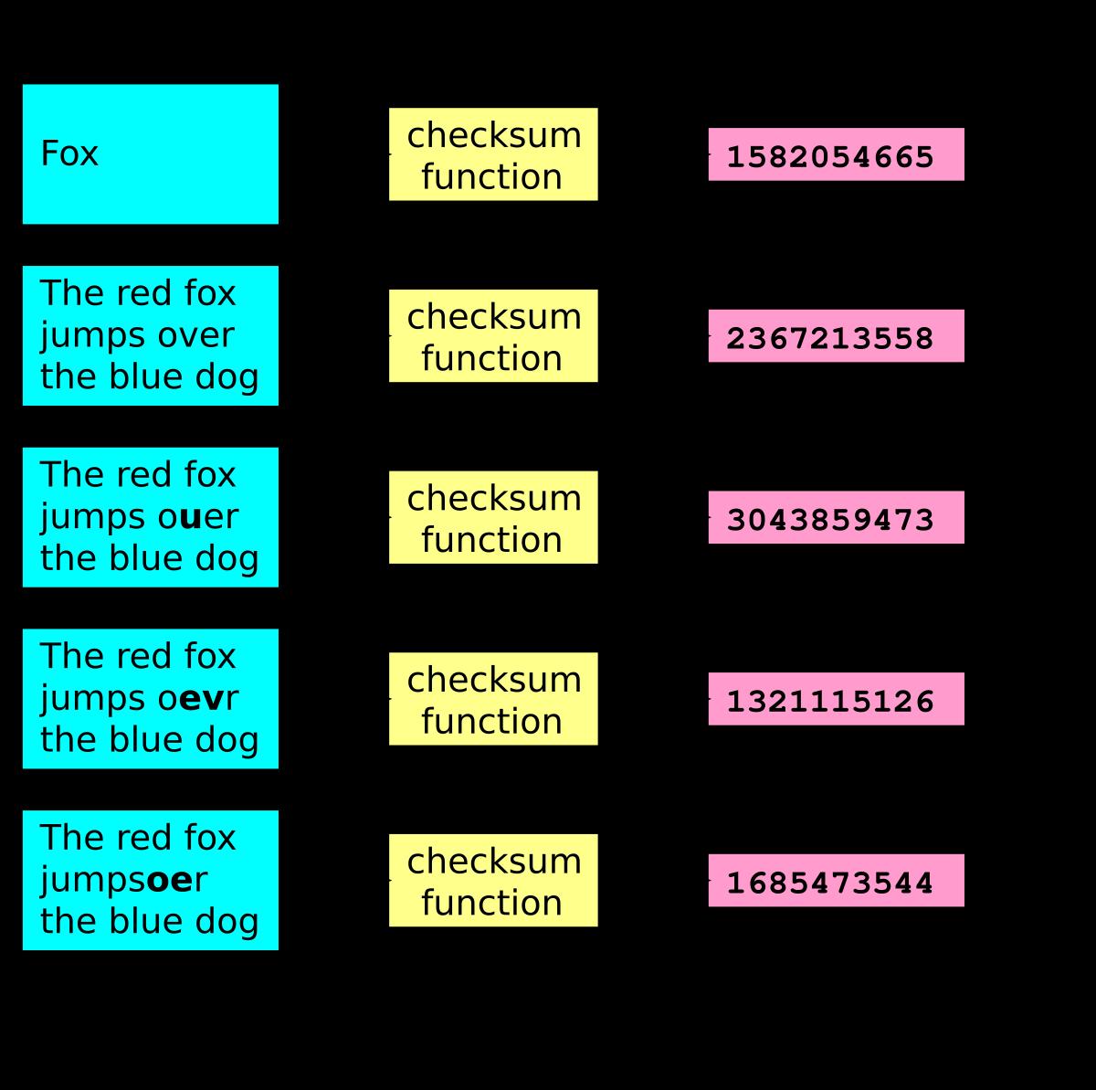
- Checksums: To detect errors in data transmission, microcontrollers calculate checksums a simple mathematical sum of the data being sent. If the receiver ’s checksum doesn’t match, the data is retransmitted This is common in serial communication, like USB or Bluetooth
- Encoding and Decoding: Math underpins encoding schemes like Manchester encoding, which synchronizes data transmission between devices This is critical in wireless systems, such as keyless car entry, where timing must be precise
These mathematical methods ensure data integrity, even in noisy or unreliable conditions
10 Real-World Examples
- Washing Machine: The microcontroller in a washing machine is first responsible for responding to the user ’s feedback when they press the machine’s buttons selecting their mode and type Afterwards, uses math to calculate the optimal spin cycle based on load size based off of the feedback given to it.
- Irrigation Systems: Automated irrigation relies on microcontrollers and sensors to detect the soil moisture & pH levels to detect when crops need water the most. In the microcontroller ’s code, when the sensors detect a value below a certain threshold, a valve is opened, allowing for the optimal time frame to water crops so as to reduce water waste from excess runoff and evaporation
- Drones: A drone’s microcontroller relies on complex math to stabilize its flight It processes data from gyroscopes and accelerometers, which detect velocity, acceleration, angular speed, and many more while using algorithms to adjust motor speeds and maintain balance mid-air.
11 Conclusion
Mathematics is the backbone of microcontroller functionality From basic binary operations to advanced control algorithms, math empowers these tiny devices to perform complex tasks with precision and efficiency Whether you’re programming a simple LED blinker or designing a sophisticated control system, understanding the math behind microcontrollers is key to unlocking their full potential
So, the next time you use a smart device be it a thermostat, a fitness tracker, or a car remember: mathematics works quietly behind the scenes to make it all happen
A Markov Chain, named after Andrei Andreevich Markov (1856-1922), is a mathematical model that describes a system that transitions between various states in a probabilistic manner. The defining property of a Markov Chain is that the future state depends only on the current state and the rate of transition from one state to another remains constant in the system. In practical terms, this means that given the present, the future is independent of the past.
In mathematical notation Markov Property is defined as follows:
Let {X0, X1, X2, . . .} be a sequence of discrete random variables. Then {X0, X1, X2, . . .} is a Markov chain if it satisfies the Markov property:
P(Xt+1 =s t+1 | Xt=st , Xt-1=st-1 , . . , X0=s0) = P(Xt+1 =s t+1 | Xt=st), for all t=1, 2, 3, . . and for all states s0, s1, . . , st , s t+1.
The system is represented by a transition matrix, P, where each element Pij represents the probability of moving from state i to state j. If v represents the current state distribution and P is the first order transition matrix, the distribution of the next step (one order higher) after one step is given by:
This process of raising the transition matrix to higher power can be repeated to predict the state distribution after several steps. N-step (nth-order) transition matrices help us to find the probability of that transition occurring over multiple steps. Markov Chains are widely used in fields such as machine learning, economics, genetics, and game theory. They can model a wide variety of systems where the outcome evolves step by step, and the probability of the next state depends on the current state.
2. Data Discussion and Frequency Matrix
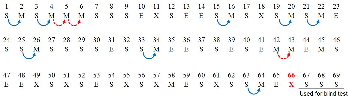
In this project, we apply the Markov model to a survey of favorite class, where respondents chose among four possible classes/states: Mathematics (state M), English (state E), Science (state X), and Social Studies (state S) and submitted the replies within a period of 76 hours We conducted a Markov Chain analysis using the first 65 transitions and reserve the last three transitions (XèS, SèS, and SèS) for a blind test to verify the prediction of the first 3 orders prediction.
The raw data of favorite class survey in sequence showing the 8 transitions from state S to M and 3 transitions from state M to M:
Based on the 65 transitions of the first 66 replies we constructed a frequency matrix showing the number of transitions between the four possible states based on the sequence of survey responses:
Current state Next state
This matrix shows how many times respondents transitioned from one state to another:
• Rows represent the starting state (e.g., respondents were in state M initially).
• Columns represent the next state respondents transitioned to.
• The total row and column give the number of times each state was a starting or ending state, respectively.
3. Markov Chain Analysis
3.1 Building the Transition Matrix (first, second and third order)
A transition matrix is a table of probabilities that describe how likely the system is to move from one state to another. We obtain the transition matrix by normalizing the frequency matrix, i.e., dividing each entry in a row by the row total (the sum of transitions from that state).
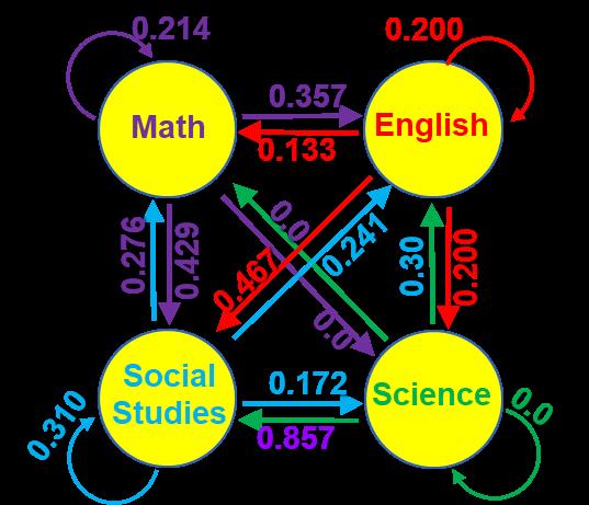
Here is the first order transition matrix derived from the frequency data alongside with its digraph:
Next state
Current state
This First order matrix shows the following:
• From state M: 21.4% chance of staying in M, 35.7% chance of transitioning to E, and 42.9% chance of moving to S.
• From state E: 13.3% chance of moving to M, 20.0% chance of staying in E or transitioning to X, and 46.7% chance of moving to S
• From state X: Dominated by an 85.7% chance of transitioning to S and a small 14.3% chance of moving to M.
• From state S: 27.6% chance of moving to M, 24.1% of transitioning to E, 17.2% of moving to X, and 31.0% chance of staying in S
Second order transition matrix calculated by raising the first order transition matrix to the power of 2:
Next state
Current state
Third order transition matrix calculated by raising the first order transition matrix to the power of 3:
Next state
Current state
3.2 Prediction Using the Markov Chain
To predict the three transitions after the last data (66th data) of X, we start with the X as the initial state. In the first order of transition, we look at the row of X and evaluate the probability of moving from X to the 4 states as follow:
1. First order Transition: From the transition matrix, the probabilities of moving from X are:
o M: 14.3%
o E: 0.0%
o X: 0.0%
o S: 85.7%
Therefore, the most likely next state of first transition from initial state of X is S with an 85.7% probability.
2. Second order Transition: Using the second order transition matrix and the initial state of X, the probabilities of moving two levels from 66th data X are:
o M: 26.7%
o E: 25.8%
o X: 14.8%
o S: 32.7%
Therefore, the most likely next state of second transition from intital state of X is S with an 32.7% probability.
3. Third Transition: Using the third order transition matrix and initial state of X, the probabilities of moving three levels from 66th data X are:
o M: 20.3%
o E: 22.6%
o X: 10.8%
o S: 46.3%
Therefore, the most likely next state of third transition from X is S with an 46.3% probability.
In summary, the predicted next three states from the initial state of X are S, S, S.
4. Blind Test Validation
To validate the Markov Chain model, we use a blind test where we predict the next three transitions and compare them to the actual observed transitions in the dataset. In this case, the actual transitions are X-S, S-S, and S-S.
The model predicted the next three states as S, S, S, which aligns perfectly with the actual observed transitions. This demonstrates that the Markov Chain model effectively captures the system’s dynamics in this case and can predict future states based on the transition matrix.
5. Applications of Markov Chains
Markov Chains are frequently used in predicting text and natural language processing, financial markets, inventory management and weather forecasting.
In natural language processing, Markov Chains are used to predict the next word in a sentence based on the current word. This is the underlying principle behind predictive text, autocompletion, and language models.
Markov Chains are used to model transitions between different market states, such as bull and bear markets. This helps in predicting future market conditions and making informed investment decisions.
In supply chain and inventory management, Markov Chains help model the movement of stock between different states (e.g., out of stock, in stock, overstocked) and predict future inventory needs.
Meteorologists use Markov Chains to model weather patterns and make weather forecasting based on current data.
6. Conclusion
In this report, we used a Markov Chain to model survey response transitions between four states Math (M), English €, Science (X), and Social Studies (S). By constructing a transition matrix and using it to predict future states, we demonstrated the effectiveness of Markov Chains for modeling probabilistic transitions. The model accurately predicted the next three states in a blind test, showing its predictive power.
Markov Chains are powerful tools with a wide range of applications, from customer behavior analysis to weather forecasting and financial modeling. The key insight is that by understanding the current state, we can make accurate predictions about future states using simple yet robust probabilistic models.
7. References
Wu, J. A, (2022). AP Statistics Survey Project, Food and Class Choices. Youtube. https://www.youtube.com/watch?v=2VxaA2-wfSM&t=4s
Gabriel's Horn Paradox: The Coexistence of the Finite and the Infinite
Doyeon(Jessica) Kim 70710 @ jisedu or id
Pure Mathematics
Key Concept: Integration
1. Introduction
Imagine a shape that can be completely filled with paint, yet its surface can never be fully covered. This is the paradox of Gabriel’s Horn, a mathematical object with finite volume but infinite surface area How can something be filled but never fully painted? This strange result can be explored by understanding infinity and the beauty of calculus.
Figure 1: The graphical representation of Gabriel’s Horn (“Gabriel’s Horn”)
2. Calculating the Finite Volume
Figure 1 shows the Gabriel’s horn, a 3D shape formed by rotating the function y = around 1 � the x-axis. This transformation creates a solid that extends infinitely along the x-axis. Despite its infinite length, Gabriel’s Horn has a finite volume but an infinite surface area To explore this, we begin by calculating its volume.
First, we define the base function over � = 1 � the interval . When this curve is � ∈ [�, �] resolved around the x-axis, it forms Gabriel’s Horn. The method of solids of revolution allows us to determine its volume
A solid revolution is a three-dimensional shape formed by rotating a two-dimensional region around a fixed line. (Mathcentre) To calculate the volume, we divide the region into thin vertical slices, each with a small width x The height of each slice is determined by the function y, which varies with x. By breaking the area under the curve into smaller regions, we observe that as x becomes smaller, we can express the sum of the area as . � � ∫ ���
The sum of the areas of these thin slices approaches the integral representation of the volume The volume of a cylinder is As π�2ℎ, the radius is and the height is x, the 1 � volume of each cylinder can be expressed as � = Σπ( 1 � ) 2 ��.
As the gets smaller by dividing the horn into �� small pieces, we can express the sum of the cylinders as It is hard to determine π 1 ∞ ∫ 1 � 2 �� the range of infinity; therefore, we need to focus on how the volume changes as t approaches infinity Below is the equation that we need to calculate
Using the power rule, we can ∫ � � = 1 �+! � �+1 , rearrange the equation; � ∞ lim → π[ � 1], 1 ≤ � ≤ �
Now, we can evaluate the definite integral by subtracting f(1) from f(t) = � ∞ lim → π [( 1 � ) ( 1)]
As t goes to infinity, it becomes zero 1 � = π [ 0 ( 1)] = π
Therefore, we prove that the Gabriel’s horn has a volume , which is a definite value π
3. Calculating the Infinite Surface Area
We’ve already seen that Gabriel’s Horn has a finite volume, but now let’s explore its surface area
Before, we only looked at , the small width of �� each piece But now, to measure the surface area, we’ll also look at s, representing each � small slice's slanted edge