3 Tradeoffs for ballistic atmospheric reentry

International Research Journal of Engineering and Technology (IRJET) Volume: 07 Issue: 09 | Sep 2020 www.irjet.net e-ISSN: 2395-0056 p-ISSN: 2395-0072

4. To design a suitable thermal protection system for surviving the reentry.

2 LITERATURE SURVEY

2.1 Atmospheric reentry

After undertaking the intended mission in the earth orbit, some spacecraft or a module of the space craft is designed for entering into the earth’s atmosphere and returningback safely to earth. The mission could be a manned mission or a sample return mission. The atmospheric re-entry could be ballistic, lifting or propulsive in nature. For Earth, atmospheric entry occurs by convention at an altitude of 120 km above the surface.

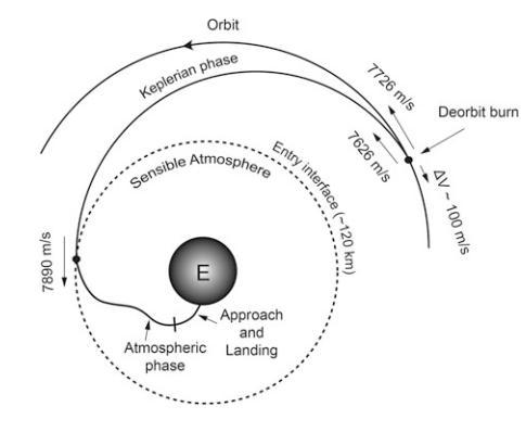
The fundamental design objective in atmospheric re-entry of a spacecraft is to dissipate the energy of a spacecraft that is traveling at hypersonic speed as it enters an atmosphere such that equipment, cargo, and any passengers are slowed and land near a specific destination on the surface at zero velocity while keeping stresses on the spacecraft and any passengers within acceptable limits. This may be accomplished by propulsive or aerodynamic (vehicle drag characteristics) means, or by some combination [2]. Typical reentry of a spacecraft from orbit till landing is shown in Figure 2.1.

Fig 2.1: Phases in reentry trajectory[2]

2.2 Types of reentry 2.2.1 Ballistics re-entry

Aballistic re-entryis one in which the entry module does not develop any lift and the only forces acting are gravity and aerodynamic drag.A capsule in ballistic re-entry has to shed speed quickly to get to the ground safely. Instead of a long, flat flight profile, a ballistic re-entry is steep and short. The drag force slows the vehicle till parachutes can be deployed for a soft touchdown. This is very different from a “controlled descent " associated with lifting reentry. The capsule's steep re-entry angle creates the atmospheric drag needed to slow down a fast-moving space capsule. The size of the corridor depends on the three competing constraints deceleration, heating, and accuracy. The landing point is predetermined by initial conditions of the entry when it starts entry to the atmosphere, and no control over the spacecraft is available once it begins the ballistic entry. In general, early manned flights like Mercury capsule[3], ISRO’s SRE (Space capsule Recovery experiment) [4] and interplanetary sample return capsules such as Stardust [5] and Genesis[6] followed ballistic reentry trajectory during their entry to earth’s atmosphere.

2.2.2 Semi-ballistic re-entry

An alternate re-entry approach is the semi-ballistic trajectory. In this case, the vehicle descends through the atmosphere till vehicle achieves the aerodynamic control capability. Appropriate control method is then used to generate lift in order to keep the vehicle within the specified limits mechanical and heat loads. The spacecraft slows down gradually with controlled lift profile until it is safe to descend it to the planetary surface. The primary design parameter for lifting entry is the Lift to Drag Ratio, or . For semiballistic entry, the ratio is nearly 0.2 to 0.3. Such low values of produce moderate g loads, moderate heating levels, and low maneuverability. Manned space capsules like Apollo [7] followed semi-ballistic entry trajectories to a splashdown at sea. Russian Soyuz[8] and Chinese Shenzhou [9] capsules continue to use semi-ballistic entry paths and usually touchdown on land.

2.2.3 Lifting re-entry

Another re-entry approach is the lifting trajectory in which the spacecraft flies through the atmosphere similarly to an aircraft. The spacecraft enters the atmosphere at a high angle of attack and generates aerodynamic lift that allows it to travel further downrange than semi-ballistic vehicle. High values of produce very low g loads, but entries are of very long duration and have continuous heating. An example is Space Shuttle re-entry at an value of around unity with a total entry time of about 25minutes. The main advantage of this technique is that the vehicle has more control over the trajectory and can perform precise landing. A further advantage is that the vehicle would typically be landed intact on a runway and can possibly be reused again. This technique is true in case of Space Shuttle [10], the only vehicle that used a lifting entry trajectory returning from orbital mission.

In the present study, more emphasis is given on the ballistic reentry trajectory design of spacecraft entering from low earth orbit (LEO) of 350km circular orbit in the equatorial plane.

2.3 Tradeoffs for ballistic atmospheric reentry

When the reentry mission begins, the entry module possesses both kinetic (by virtue of its velocity) and potential energies (by virtue of its altitude). During reentry, this energy stored by the entry module need to be completely dissipated, aerodynamic drag encountered by the module during its reentry utilized to dissipate this energy and bringing the module back safely to the ground. This is the most efficient way of dissipating the energy of thereentry module. But this way of dissipating the energy,

International Research Journal of Engineering and Technology (IRJET) Volume: 07 Issue: 09 | Sep 2020 www.irjet.net e-ISSN: 2395-0056 p-ISSN: 2395-0072

introduces two major challenges for the module design as given below.

2.3.1 Deceleration load

As the module nears Earth’s atmosphere, the drag force at higher altitude is not sufficient to dissipate the energy, hence the entry module penetrates the atmosphere at very high velocity nearly equal to the orbital/ interplanetary velocity. This causes a sharp increase in the aerodynamic loads acting on the vehicle structure.

The vehicle’s structure and payload limit the maximum deceleration or “g’s” it can withstand. (One “g” is gravitational acceleration at Earth’ssurface-9.798 . The maximum deceleration a vehicle experiences during reentry must be low enough to prevent damage to the weakest part of the vehicle. Deceleration builds gradually to some maximum value , and then begins to taper off.

2.3.2 Peak Aerodynamic Heat Flux and Heat Load

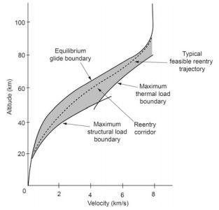
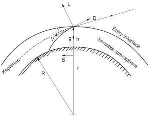
Vehicle reenters the atmosphere with very high kinetic energy due to speed almost equal to the orbital speed. During the process of energy dissipation, the kinetic energy of the vehicle is converted into thermal energy. As an example, for a return mission from low Earth orbit (LEO), the vehicle reenters the atmosphere with the velocity of about 8 km/s whereas for the return from lunar and interplanetary missions, the vehicle reenters the Earth atmosphere with the velocities of about 11 km/s and 16.4 km/s respectively. From aero-thermodynamic point of view, these are the free stream hypersonic velocities of air particles with respect to the vehicle when it reenters the atmosphere. The strong normal shock generated by the hypersonic flow, standing in front of the vehicle, compresses and slows down the air particles and in this process, the internal energy of the air particles increases. In this energy conversion process, the aerodynamic drag force reduces the speed of the vehicle. Further the kinetic energy of air particles is dissipated and in turn the internal energy is increased. For the case of perfect gas, the internal energy increase is in the form of increasing the temperature of air particles i.e., the entire energy is converted into temperature rise of air particles between shock wave and front portion of the vehicle. This hot air baths over the entire body of the vehicle behind the shock wave and through heat transfer mechanisms viz. convective and radiative transfer process, the thermal energy is transferred to the vehicle body. Fig 2.6: Feasible trajectory of a re-entry module [2]

For the reentry from LEO, the heat transfer through convection of hot air flow process is crucial. For the case of reentry with higher velocity as in the case of lunar or interplanetary return missions, the temperature of hot air is sufficiently high, in addition to the convective heating process; the heat transfer to body through radiative process is also higher.

Generally, for a ballistic re-entry, the peak aerodynamic heat flux is higher and the total heat load is lower compared to other modes of entry. Peak aerodynamic heat flux decides the TPS material choice and total heat load decides the TPS thickness and its mass. So, for a ballistic reentry design, tradeoff has to be made between the above two factors deceleration load and aerodynamic heat flux. Figure 2.6shows how a feasible reentry trajectory of a reentry module is designed.

2.4 Heat flux estimation

The best method for predicting aerodynamic heating is viscous computational fluid dynamics (CFD) solutions. CFD provides a direct means of computing heat flux. However, these methods require large computer run times and storage, and each time the flight conditions change (e.g. the Mach number, altitude and angle of attack) a new computer run must be made. Therefore, using CFD to calculate complete time histories of transient temperatures and heat flux becomes very expensive and time consuming.

However, for design purposes, we can use approximate engineering methods based on boundary layer theory. These methods give fairly accurate and conservative estimates of heat transfer over a wide range of flow conditions. Software’s such as MINIVER [11], TPATH [12] developed by NASA and OTAP developed by ISRO use such engineering methods for estimating transient aerodynamic heat flux.

2.4.1 Heat Flux Correlations for Convective Heat Flux estimation 2.4.1.1 Fay-Riddell correlation [13]

Fay and Riddell established a simple correlation formula for finding the stagnation-point convective heating for a vehicle (equation 2.2)

International Research Journal of Engineering and Technology (IRJET) Volume: 07 Issue: 09 | Sep 2020 www.irjet.net e-ISSN: 2395-0056 p-ISSN: 2395-0072

(2.2) Where,

Where is the convective heat flux, ρ is the density, μ is the absolute viscosity, L is the Lewis number for atom-molecule mixtures (Lewis number being the ratio of thermal diffusivity over mass diffusivity), is the average atomic dissociation energy times atom mass fraction in external flow, h is the enthalpy per unit mass of mixture, u is the x component of velocity, x is the distance along the meridian profile. The Subscript e indicates external flow conditions, w indicates wall and s indicates the stagnation point for the external flow. P is pressure, R is the nose radius. Subscript ∞ indicates free stream. Fay-Riddell correlation is a bit complicated that the Lewis number needs to be calculated in order to solve for the convective heating.

2.5Thermal Protection System (TPS)

TPS is simply known as thermal protection system and are used when a spacecraft enters any planetary atmosphere, high energy, high velocity flights through planetary atmospheres lead to extremely severe aerodynamic heating and pressures on the vehicle exteriors. The vehicle structure needs to be insulated using suitable TPS to keep the structure within temperature limits.

TPS forms the external surface of a vehicle and is exposed to a variety of environmental conditions at different times during its flight. The specific times and nature of these conditions differ for different missions and vehicle type. The aerodynamic heating and pressure experienced by a TPS are also dependent on the vehicle shape and the trajectories taken by the vehicle.

2.5.1 TPS Types

Type of TPS and specific designs can depend on the magnitude and duration of aerodynamic heating. Even on the same vehicle several different TPS may be used, as the heating varies over thevehicle surface. TPS approaches can be broadly classified into 3 categories, they are as follows,  Passive TPS: Passive TPS radiate the heat from top surface and/or absorb heat into the structure during high heating periods and dissipate it after the heating subsides. Passive TPS have no working fluids to remove or dissipate heat. Passive systems have the simplest designs and are suitable for low heat loads. For high heat loads the weight of the passive TPS becomes prohibitively high.  Semi-passive TPS: Semi-passive TPS use a working fluid to remove heat from the TPS but require no external system to circulate the fluid. Two of the most © 2020,  . 0.1 0.4 0.520.94( ) ( ) 1 ( 1) eD C w w s s s w ss duh q L h hh dx                            21 se s s P Pdu dx R              cqDh IRJET | Impact Factor value: 7.529 |

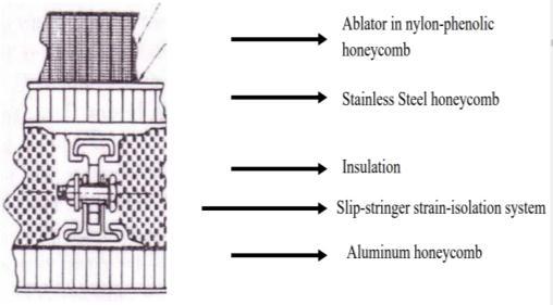
frequently discussed semi-passive TPS concepts are heat pipes and ablators. Heat pipes are suitable for regions where thereis extremely high, localized heating close to a cooler region. Ablators are very practical and attractive concepts for thermal protection and were extensively used on space capsules like Apollo and Soyuz. Ablators undergo chemical changes by absorbing theaerodynamic heat and generate gases, thus, blocking the majority of the heat from reaching the vehicle surface. The Apollo heat shield structure is shown in Figure 2.7. In order to increase the ablator tensile strength, it was injected into a fiberglass reinforcednylon-phenolic honeycomb structure, which was bonded to a brazed stainless-steel honeycomb structure. Active TPS: Active TPS have an external system that supplies coolant to continually remove heat or to block the heat from reaching the structure. There are three commonly discussed active TPS concepts. 1. Transpiration, 2. Film and 3. Convective Cooling. In transpiration and film cooling a fluid is ejected from the vehicle surface, which flows along the surface and evaporates by absorbing the aerodynamically generated heat, thus, preventing the heat from reaching the surface of the vehicle. Convective cooling is a more practical TPS concept. In this concept, a coolant is circulated through passages in the airframe to remove heat that has been absorbed from aerodynamic heating.

Fig 2.7: Apollo heat shield structure [15]

2. 6 Inflatable Aerodynamic Decelerator (Ballute)

In general, large drag area or low ballistic coefficient (β) is preferable to slow down the entry module early during its reentry,but for rigid aeroshell the size is limited by the payload fairing of launch vehicles. This size limitation of the traditional rigid aeroshell results in lower drag area and high β, this causes deceleration at low dense atmosphere resulting in very high heat flux and deceleration loads. This results in high TPS mass fraction, again drastically affecting the useful payload. Due to their above limitations, conventional rigid aeroshell systems are rapidly approaching the payload limit that the technology can deliver while fitting within the payload fairing of existing launch vehicles. But for future crewed missions, sample return missions and exploration of outer gas giants, the traditional rigid aeroshell may not be an optimum option. The Inflatable Aerodynamic Decelerator (IAD) addresses these limitations of rigid aero shell.

International Research Journal of Engineering and Technology (IRJET) Volume: 07 Issue: 09 | Sep 2020 www.irjet.net e-ISSN: 2395-0056 p-ISSN: 2395-0072

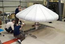
Fig 2.8: NASA IRVE-3 [16] Compared with traditional rigid aeroshells, IADs are made of lightweight flexible materials that can be packaged into a smaller volume in the rocket fairing and inflated upon reentry. This enables a reduction in the ballistic coefficient of an entry vehicle through an increase in drag area, in exchange for a minimal mass impact compared to a rigid vehicle of the same size. This reduction in ballistic coefficient, due to large drag area enables deceleration at higher altitudes allowing reduced heat rates, access to higher elevations and an increase in delivered payload.

The size of the inflatable/deployable aeroshell is not limited by the payload fairing diameter. Inside the PLF, the inflatable/deployable aeroshell will be in stowed condition, after separation it will be inflated or deployed to a larger diameter to increase the drag area. The concept is depicted in Figure 1.1.

Besides advantages such as stowage in compact space, light weight material used increases the payload mass fraction. Hence IADs are envisaged worldwide as an essential technology for many future planetary entry missions. NASA IRVE-3 is an IAD technology demonstrated in a sub orbital reentry (shown in Figure 2.8).

2.6.1 Types of IADs

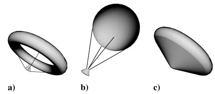
There are three distinct IAD configurations are shown in Figure 2.9

Trailing Torus: It consists of an inflated ring, attached to the entry vehicle by a series of tethers. The trailing sphere, the simple sphere is replaced by torus shape.

The trailing torus have higher ballistic coefficient and provides in reduced surface area over the clamped version is insufficient to overcome its significantly lower drag contribution. Fig 2.9: IAD Configurations: a) Trailing Torus, b) Trailing Sphere, and Clamped Torus [17] Trailing Sphere: It has lower ballistic coefficient compare to the others. Trailing Sphere may require less material and pressuring, less massive. A large trailing sphere may produce as much drag as a medium sized clamped torus. Clamped Torus: The clamped torus does away with tethers and instead attaches the torus to the entry vehicle with a conical frustum that fully encloses the vehicle. These configurations offer advantages in the heating regime. Heating results on the clamped ballute were the most favorable. Because the clamped ballute is attached directly to the base of the vehicle.

2.7.2 Applications

 The IADs has been used as a retarding device for freefall bombs dropped from aircraft.  It was used as part of the escape equipment for the

Gemini spacecraft.  It has been proposed for use during aero capture and aero braking for Mars mission.  Extended designs using inflatable tension cone ballute technology have been proposed for de-orbiting

NanoSats and recovering low-mass (< 1.5 kilograms (3.3lbs.) satellites from low Earth orbit[18]

3. TRAJECTORY ANALYSIS 3.1 Trajectory equations

To determine the re-entry heat flux and the deceleration loads on ballistic re-entry vehicle, the trajectory must be ascertained first. In this chapter, the equations for the trajectories of ballistic re-entry will be derived.

3.1.1 Governing equation

The main governing equation in flight mechanics is Newton's second law,

3.1.2 Coordinate system

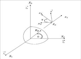
First on the list is defining a coordinate system. This is introduced to make a clear-cut idea of how a reentry vehicle enters our atmospheric space through coordinate systems. We still need an inertial reference frame, which we call the re-entry coordinate system. To make things easy, we place the origin of the re-entry coordinate system at the vehicle’s center of mass at the start of re-entry. We then analyze the motion with respect to this fixed center. Figure 3.1 gives the details of re-entry co-ordinates system and the

position of the vehicle at the time of its re-entry. © 2020,F ma  3.1 IRJET | Impact Factor value: 7.529

International Research Journal of Engineering and Technology (IRJET) Volume: 07 Issue: 09 | Sep 2020 www.irjet.net e-ISSN: 2395-0056 p-ISSN: 2395-0072

Fig 3.1: Re-entry Co-ordinate system

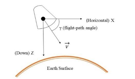
The fundamental plane is the vehicle’s orbital plane. Within this plane, we can pick a convenient principal direction, which points “down” to Earth’s center. (By convention, the axis that points down is the direction.) We define the direction along the local horizontal in the direction of motion. The direction completes the righthand rule. However, because we assume all motion take place in plane, we won’t worry about the direction. Figure shows the re-entry coordinate system. Fig 3.2: Planar motion of re-entry body [19] Figure shows a re-entry body (RB) at some point on an exo-atmospheric trajectory. We have established an axis system whose origin coincides with the RB. The coordinate frame axes are set as follows: "up" along the geocentric vector ; north, and to the west, completing the right-handed triad. A fixed, or inertial, axis is located at the Earth's center, with along the polar axis and and in the equatorial plane. Note that when the central angle 0 (essentially the latitude) is zero, both axis sets are parallel. moving frame and the plane of the inertial frame. The radius vector makes the angle with respect to the equatorial plane. The velocity vector makes an angle with respect to the axis. The angle γ, the flight path angle, is considered positive for a velocity vector above the horizontal.

3.1.3 Assumptions

Earth is assumed to be a spherical Earth’s rotation is stationary during the re-entry period. Coefficient of drag, is constant throughout the re-entry. Re-entry is assumed be two dimensional in the equatorial plane Mass of the spacecraft during the entire re-entry is assumed to be constant. Mass loss due to propulsion and ablation is neglected. Re-entry body is assumed to be a point mass and all the forces acts on the C.G of the spacecraft. Figure 8 shows the free-body diagram for the spacecraft

The velocity vector V is confined to the plane of the

during re-entry.

© 2020,Z X Y 3.1 3.2 1xER 2 x3x 3X1X2X1 2( , )x x2 3( , )X X2xDC sin dV m D mg dt    (3.2) 2 cos d V mV L m gdt r            (3.3) sin dr dh V dt dt    (3.4) 21 2 DD V SC  (3.5) 21 sin 2 D dV m V SC mg dt            (3.6) mg 21 2 sin D VdV gdt mg SC                                       (3.7) D mg SC  IRJET |

Fig 3.3: Free body diagram of spacecraft during re-entry [2]. Writing the equations in two dimensions[20], balancing the forces,

Substitute equation in and rearranging,

Dividing by

and rearranging,

The factor in equation is called ballistic coefficient,

The above equations are expressed as a derivative of time. Convert all the above equations as a function of altitude. This is done for making our calculations easier and for further simplification.

International Research Journal of Engineering and Technology (IRJET) Volume: 07 Issue: 09 | Sep 2020 www.irjet.net e-ISSN: 2395-0056 p-ISSN: 2395-0072

Divide equation (3.7) by (3.4)

We have to calculate the time duration at the time of re-entry

For a ballistic entry, lift and rearranging, , substituting in equation

But , substituting in equation

Correspondingly by dividing the above equation with

equation, (3.4) we get The time interval can be calculated by taking the reciprocal of equation (3.4) So, equation and 3.12 are the three equations which need to be solved numerically to find the re-entry trajectory.

3.1.4 Euler’s method for numerical integration

The closed-form solutions are excellent for providing rapid estimations of the design parameters; numerical integrations will be required when refinements are necessary for final design. A simple Euler's method may be used to numerically integrate this set. They are, Re-arranging, Correspondingly, the flight path angle is

3.1.5 Initial conditions

Trajectory design involves defining the re-entry initial conditions. These initial conditions are thevelocity, ,

altitude , and flight-path angle, at the start of re-entry.

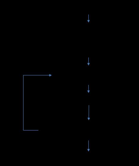
3.2 Flow chart for trajectory program

Fig 3.4 gives the process flowchart we adopted for designing the trajectory program and computing the

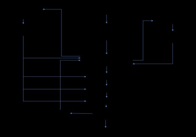
associated parameters.

© 2020, 21 2 V Sin dV g dh VSin                     3.80L  3.3 21 cos d V g dt V r          (3.9) ( ) E r R h     21 cos E d V g dt V R h             (3.10) 2 E 2 V cos γ g R hd dh V sin γ            (3.11) 1 sin dt dh V    (3.12) 3.8, 3.11      21 2 sin sin V g V h h V h h V                 3.13    21 2 sin sin V g V h h V h h V                                3.14    2 2 cos sin E V g R h h h h h V                       3.15    1 sin t h h t h h V           3.16 e V e h e IRJET |

Fig 3.4: Flowchart for trajectory program

The flowchart given above is a visual representation of the sequence of steps and decisions we have taken to performing the process of TPS design

Flow chart mainly include three sections, they are

The atmospheric model Gravity model Trajectory design.

Using atmospheric model, we calculated the pressure, temperature, and density, in which the temperature lapse rates are taken from the combination of standard atmosphere 1976 and 1962. Similarly, from the gravity model we calculated acceleration due to gravity (each altitude) for the trajectory calculation.

With the initial conditions specified in section 3.1.5, the trajectory equations given in section 3.1.4 is solved using Euler’s method for every increment altitude of 10m. Density at every altitude required for trajectory computation is derived from the atmospheric model. And gravity at every altitude is derived from gravity model. We get Velocity, altitude, time and entry flight path angle as the output from the trajectory program.

International Research Journal of Engineering and Technology (IRJET) Volume: 07 Issue: 09 | Sep 2020 www.irjet.net e-ISSN: 2395-0056 p-ISSN: 2395-0072

Additional parameters such as Mach number are calculated by taking temperature from atmospheric model and velocity from the trajectory. Similarly, for calculating the Reynolds number, density and temperature are taken as an input from atmospheric model and velocity from trajectory. We also calculated the heat flux using empirical correlations (details are given in chapter 5). Density from Atmospheric model and Velocity from trajectory are the inputs for computation of heat flux.

3.3 Atmospheric model 3.3.1 Standard atmosphere

There are mainly two versions of standard atmosphere model

1. 2. Standard atmosphere model 1962[21] Standard atmosphere model 1976[21]

Standard Atmosphere is a single mapping of primary properties (pressure and temperature) and derived properties (density, viscosity, speed of sound propagation, mean free path length, etc.) with altitude, which by international agreement for historical reasons is roughly representative of year-round mid-latitude conditions [21] .

These are basically used for pressure altimeter calibrations, aircraft performance calculations, aircraft and rocket design, ballistic tables etc. At a time for calculating these either of the standard atmosphere models should be considered. But here we follow the standard atmospheric model 1976 till an altitude of 86 km and from 86km to 120km we are adapting U.S. Standard Atmosphere model 1962.

The atmosphere shall also be considered to rotate with the Earth and the air is assumed to obey the perfect gas law and the hydrostatic equation, which taken together relate temperature, pressure, and density with geo-potential altitude.

The U.S. Standard Atmosphere is an atmospheric model that meets the conditions set forth by World Meteorological Organization (WMO) [22]. Based upon the atmospheric model and assumptions; generating equations for geometric and geo-potential altitude, we get: Substituting above equation and re-arranging give the below equations. The molecular temperature is represented as a linear function of geo-potential altitude as our atmospheric region is divided into 7 strata;

Where the subscript i identifies the layer

Where, is known here as the thermal lapse rateas given in Table 3.1

The properties of the atmosphere over the altitude range of 86 to 700 km will vary widely because at such altitudes the atmosphere is greatly influenced by solar radiation. Above 86 km or so, the assumption of hydrostatic equilibrium is no longer valid. Because of diffusion and vertical motion of the various constituent gas species, the atmosphere above 86 km is highly dynamic.

Table 3.1 Atmosphere lapse rate and molecular temperature (US atmosphere 1976)

Layer Geometric Molecular Lapse index altitude Z, temperature Rate Km K K/km

0 0.0 288.150

-6.5 1 2 3 4 5 6 7 11.0102 20.0631 32.1619 47.3501 51.4125 71.8020 86.0 216.650 216.650 228.650 270.650 270.650 214.650 186.946 0 1 2.8 0 2.8 2

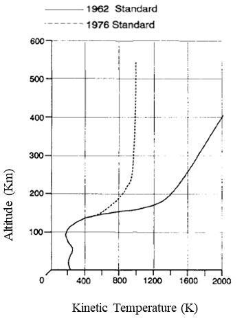
Our re-entry vehicle will be at 120 km at the time of entering the atmospheric region of space and will be facing the above-mentioned conditions. Temperature variations with altitude for the 1962 and 1976 Standard Atmospheres

Equation ,in differential form;

models are shown in Figure 3.5.

© 2020,   2 E E R h R Z Z         (3.3.1)   2 E E R dh dZ R Z         2 0[ / ( )] E E g g R R Z   0 dh g g dZ        0 g dh dZ g         I i M M h i T T L h h    0 i 7  i M h i dT L dZ  ih L IRJET |

International Research Journal of Engineering and Technology (IRJET) Volume: 07 Issue: 09 | Sep 2020 www.irjet.net e-ISSN: 2395-0056 p-ISSN: 2395-0072

Fig 3.5: Temperature variations with altitude for the 1962 and 1976 Standard Atmospheres models[16]

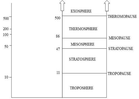
3.3.2 Atmospheric description

Atmospheric description is the basis defining the different atmospheric layers and their properties. Moving upward from the sea level, the atmosphere layers are named as the troposphere, stratosphere, mesosphere, thermosphere and exosphere. These atmospheric layers are shown in Figure 3.6. The numbers indicate altitude in km. Fig 3.6: Atmospheric strata definition[21] .

3.3.3 Physical foundation of atmospheric model

[21] For the calculation of heat flux and trajectory, we need to find the pressure, temperature, and derived density as a function of altitude. Figure 3.7 shows below depicts element in equilibrium under pressure and gravitational forces Fig 3.7 Equilibrium element under pressure and gravitational forces[21]

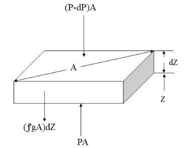
Consider the atmospheric equilibrium equation which relates the pressure P, and density . Summing both pressure and gravitational forces gives,

Differentiating,

We assume the atmosphere to be a thermodynamic fluid, then the ideal gas equation

Where the pressure P and temperature T are related to the volume V, the number of moles presents N, and the Divide Eq.

by the volume V,

universal gas constant We can express pressure and density in a form

known as the polytrophic equation of state as follows,

Where the subscript o refers to a reference condition. The linear temperature profiles have already been given in Equations, And ; these relationships are repeated below;

© 2020,   ρgAdZ P P dP dA 0         dP ρgdZ    3.3.5 * PV NR T  3.3.6 * .R * ( )PV NR T V V  3.3.7 * mR T P MV  m N M       * ( ) R T P M   3.3.8m{ ρ } V  n P ρ CONSTANT   0 0 P n  3.3.93.3.3 3.3.4  i i M M Z i T T L Z Z    3.3.10a i i M M h i T T L h h    b IRJET |

We now consider how geopotential and geometric altitudes differ. To do this we must first recognize the relationship between the altitude and the gravitational force. The geopotential altitude h is found by assuming a constant sea-level value for the gravitational acceleration throughout the entire atmosphere. It is related to the more

International Research Journal of Engineering and Technology (IRJET) Volume: 07 Issue: 09 | Sep 2020 www.irjet.net e-ISSN: 2395-0056 p-ISSN: 2395-0072

physically realistic geometric altitude Z by the following equation:

Rewriting the Eqns. logarithmic differential, and

And,

Put the equation in equation

or, divide the above equation using Then,we get The kinetic temperature has been replaced by the molecular temperature according to Eq. Equation is the relationship between the temperature gradient In developing an analytical model of the atmosphere, we eliminate the density in the equilibrium equation by using the ideal gas equation to give the following relationship between the proportional pressure change and the geometric altitude increment Then, And in terms of geopotential altitude (h), in terms of

, then we get, The next step is to integrate the above equation from the beginning of the layer to some point within the layer but below the layer. We shall carry out the integration for two cases; 1) The isothermal atmosphere where is zero throughout the layer (temperature remains constant). 2) The non-isothermal layer where is non-zero (temperature varies linearly with altitude). In both cases we consider the geometric altitude as the running, or independent,variable. First, we must express the gravitational acceleration in a form convenient for integration. We can represent the

We have,

Put the value of on equation , then Substitute equation in equation (3.17)

and the poly tropic exponent n. spherical Earth gravity field as 3.3.3.1 Isothermal layer For isothermal case , here the temperature did not vary with altitude ie, the temperature remains constant

and,

Similarly,

© 2020,g dh dz g        3.3.11 3.3.8 3.3.9dP dρ dT P ρ T   3.3.12 1 dP dρ n P ρ  3.3.13 P dZ dP n P dT dZ n 1 T dZ         3.3.14dP ρgdZ   * ρR TP M  * 1 dP PM ρ g dZ R T    3.3.15 * dP PM g dZ R T         dP * PM n P dT g TR n 1 T dZ          0m * gMdT n 1 dZ n R          3.3.16  3.3.1 . 3.3.5 dZ * PM ρ R T  * dP PM gdZ R T       0 * M M M gdZ dP gdZ dZ R T Z RT Z     * 0 R R M         3.3.17a    0 0 * M M M gdH g dhdP dZ R T h RT h     bthi i l th  ZL   2 2 E 0 2 E R g g R Z          3.3.18  0 0 E 2 g g 1 Z g 1 bZ R                 3.3.197 1 E 2 b 3.139 10 / m R             3.19    i 0 M Z I 1 bZ dZgdP P R T L Z Z        i M M Z i T T L Z Z       i i i 0 P Z M Z I 1 bZ dZgdP P R T L Z Z P Z      Z L 0    i i i 0 P Z M 1 bZ dZgdP P R T P Z     3.3.20    0 i i M g b P P exp Z Z 1 Z Z RT 2 i                 3.3.21a iM MT T  b   0 i i M g b ρ ρ exp Z Z 1 Z Z RT 2 i                 3.3.21c L 0  IRJET |

3.3.3.2 Non-isothermal layer For non-isothermal case .The temperature gradually changes with altitude.

International Research Journal of Engineering and Technology (IRJET) Volume: 07 Issue: 09 | Sep 2020 www.irjet.net e-ISSN: 2395-0056 p-ISSN: 2395-0072

By integrating, It can be written as, Final equation will be, used for the nonzero lapse rate layers.

3.4 Gravity model [21]

Gravity model deals with the assumption that the earth is in the shape of a sphere and not considered as geoid. We have taken the case of sphere to make our calculations easier. The simplest earth model is spherical with no gravity and no earth rotation. When the spherical earth model is selected, it consists of just one term, which is treating the earth as a point mass. Hence, we use the below equation for our calculations.

3.5 Other derived parameters 3.5.1 Mach number

Mach number is a dimensionless quantity representing the ratio of flow velocitypast a boundaryto the local sound. For calculating Mach number, relative velocity is directly taken from the trajectory and temperature from the calculated atmospheric model.

Equations are used for zero lapse rate (i.e., for

isothermal) layer calculations and Eqns. are

,

© 2020,   i i i 0 P Z M i 1 bZ dZgdP TP RL Z Z L i i P Z Z Z                      3.3.22    i i i i ii i i Z ZP 0 P Z Z M MZ i i Z Z g dZ ZdZ log P bT TRL Z Z Z Z L L                        3.3.23        i i i i i i ii i i i M i ZZ M M Z0 i i i Z Z MZ Z Z i Z T Z T T Lg log Z Z log Z Z b Z dZ TRL L L Z Z L                                                             3.3.24      i i i i i i i i M i Z M0 0 i i M Z Z Z i i Z T Z Z L Tbg gZ Z log b Z 1 T RL RL L Z Z L                                           i i i i i i i i i M i P Z M0 0 i iP M Z Z Z i i Z T Z Z L Tg bg log P log b Z 1 Z Z T RL L RL Z Z L                                     3.3.25       M0 i i Z Z i i i i i Tg 1 b Z RL L Z 0 i i i M Z L g b P P Z Z 1 exp Z Z T RL                                                                       3.3.26a i i M M Z i T T L Z Z    b      M0 i i Z Z i i i i i Tg 1 b Z RL L Z 0 i i i M Z L g b ρ ρ Z Z 1 exp Z Z T RL                                                                       3.3.26c3.3.21 2 E 0 E R g g R Z         V M a a γRT Inertial force Re viscous force  ρVDRe μ 

3.5.2 Reynolds Number

The Reynolds number is the ratio of inertia to viscous forces in the fluid.Inertial forceinvolves force due to the momentum of the mass of flowing fluid and the viscous forcesdeal with thefriction of a flowing fluid.

Where, D is the overall diameter of the ballute. The dynamic viscosity is a function of temperature. Therefore, we are calculating Reynolds number by taking density and temperature from atmospheric model and relative velocity from trajectory.

3.6 Validation of Atmospheric Model

Atmospheric model generated for designing the trajectory was validated against the US 1976 standard atmosphere.

U.S. Standard Atmosphere (1976)

The “U.S. Standard Atmosphere 1976” is an atmospheric model of how the pressure, temperature, density and velocity of the Earth’s atmosphere changes with altitude. Standard values for pressure, temperature and density (ignoring the slight effect of humidity) at altitudes from sea level to 200km is taken from the U.S. Standard Atmosphere data and we compare it with present calculations. Some plots like Altitude Vs Temperature, Altitude Vs Pressure and Altitude Vs Density from the U.S. Standard Atmosphere data were extracted and these plots are compared with the corresponding graphs from our atmospheric model calculations.

International Research Journal of Engineering and Technology (IRJET) Volume: 07 Issue: 09 | Sep 2020 www.irjet.net

3.6.1 Temperature Vs Altitude 3.6.3 Altitude Vs Density

e-ISSN: 2395-0056 p-ISSN: 2395-0072

Fig 3.8: Altitude Vs Temperature

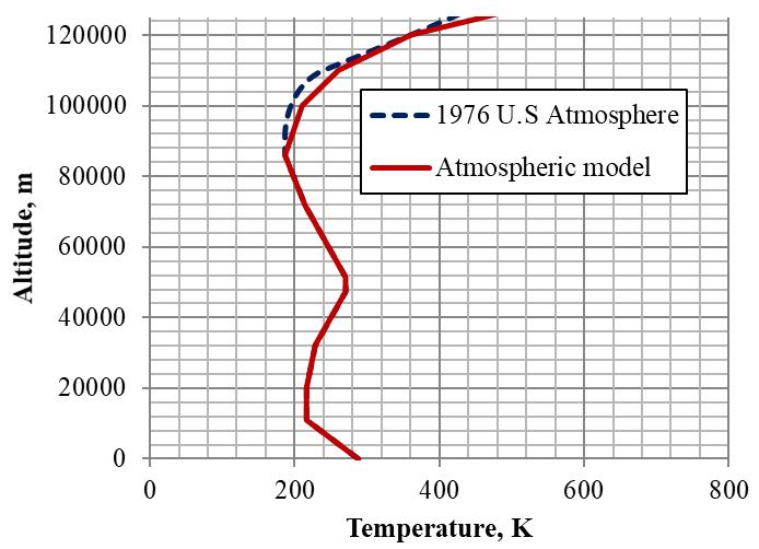
Figure 3.8 is the Altitude vs Temperature graph. From the given plot, it is very clear that the temperature variation is very similar to the US standard atmosphere (1976) up to an altitude of 90km, after that there is a marginal variation. The rate of increase in temperature with altitude is greater for present atmospheric model than the U.S. Standard Atmosphere model. This is because the lapse rate to 86km is based on U.S 1976 standard atmosphere and beyond this altitude, it is taken from US Standard Atmosphere 1962.

3.6.2 Altitude Vs Pressure

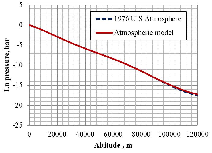
Fig 3.10: Altitude Vs Density

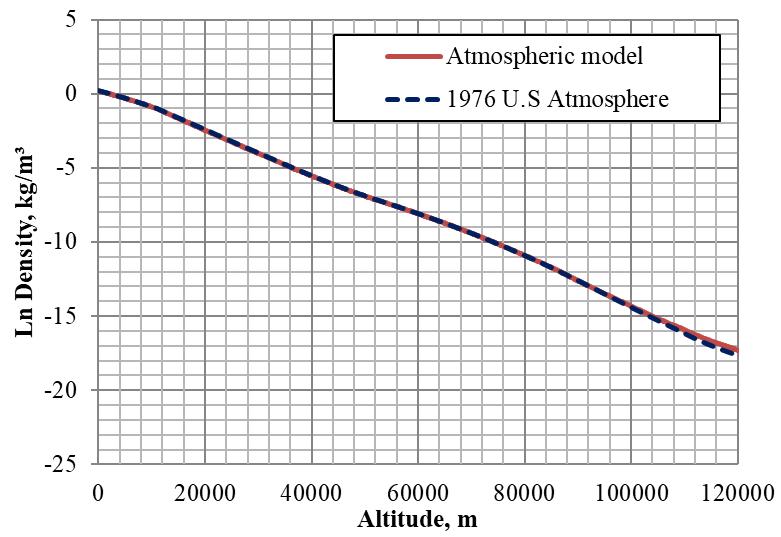
The variation of density with altitude is similar to the pressure variation. Maximum density is experienced at sea level. Hence the density increases when the vehicle is at its re-entry period. Similar to altitude Vs pressure graph, natural logarithm of density (Y= ln[density]) was taken. Fig 3.10 shows the comparison of density between US 1976 Standard atmosphere and atmospheric model. The comparison is very good.

3.7 Validation of trajectory

For validation of the trajectory program, Stardust Best Estimated Trajectory (BET) from flight [24] is compared with the estimated trajectory from the program. Also, the flight measured heat flux is compared with the heat flux obtained using empirical correlation.

3.7.1 Stardust Parameters

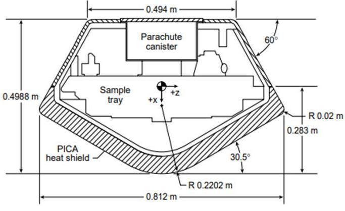
Stardust, being a ballistic re-entry vehicle i.e. with zero lift to drag ratio, enters directly into the Earth atmosphere experiencing high heat and deceleration loads. Figure 3.11 shows the geometric dimensions of stardust re-entry vehicle.

Fig 3.9: Altitude Vs Pressure

Atmospheric pressure decreases with increasing height. Since most of the atmosphere's molecules are held close to the earth's surface by the force of gravity, air pressure decreases rapidly at first, then more slowly at higher levels. Figure 3.9 is the altitude Vs pressure graph from US 1976 Standard atmosphere and atmospheric model. The plot is generated by taking the natural logarithm of pressure (Y= ln[pressure]) along the Y-axis and altitude along X-axis. Very good comparison in pressure is observed between US 1976 Standard atmosphere and atmospheric model

Fig. 3.11: Stardust re-entry vehicle[25]

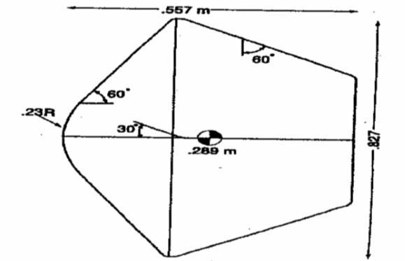
Stardust reentry parameters  Altitude-120km  Entry angle= -8.2º(inertial)  Entry velocity=12.8km/sec (inertial)  Mass =45.8 kg  BC=60kg/m²

International Research Journal of Engineering and Technology (IRJET) Volume: 07 Issue: 09 | Sep 2020 www.irjet.net e-ISSN: 2395-0056 p-ISSN: 2395-0072

Nose radius=0.23 m Base radius= 0.52 m²

3.7.2Altitude Vs Time

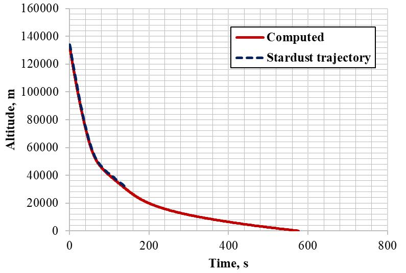
Figure 3.12 given below shows the altitude history from Stardust BET and computed trajectory using the program. Very good comparison is observed when we are taking (relative velocity) flight data. Fig 3.12: Altitude history

3.7.3 Velocity Vs Time

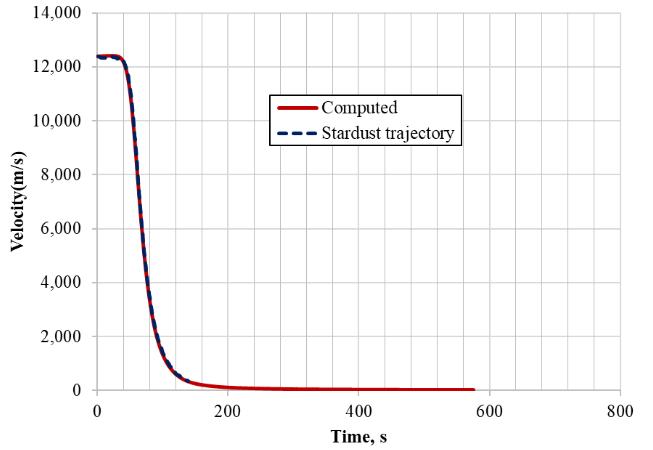
Figure 3.13 given below shows the velocity history from Stardust BET and computed trajectory using the program. Very good comparison is observed. Fig 3.13: Velocity Vs Time

4. IAD CONFIGURATION

Inflatable Aerodynamic Decelerator (IAD) enables a reduction in the ballistic coefficient of an entry vehicle through an increase in drag area. In this chapter, the IAD design parameters such as ballute diameter, torus radius etc were computed.

4.1 Methodology adopted for designing IAD configuration

For designing the IAD configuration,  Baseline entry vehicle was selected as Stardust capsule.  IAD need to be attached to the stardust entry capsule to reduce its ballistic coefficient by one order (from 60kg/m2 to 6kg/m2). For achieving the low ballistic coefficient of 6kg/m2, the IAD parameters were computed.

4.2 Stardust baseline configuration

Fig 4.1: Stardust sample return capsule configuration[24]

Stardust was the first comet sample return mission. It is the fourth of NASA’s Discovery class missions, was launched on 07 February 1999 and return to earth on 16 January 2006.The baseline geometry of the Stardust Sample Return Capsule is consisting of a 60-deg half-angle, spherically-blunted cone forebody with a 30-deg half-angle conical afterbody. The nose radius is 0.2202 m, and the overall diameter , is 0.812 m. The Earth-return stardust capsule has inertial velocity of 12.8km/s with inertial flight path angle -8.2 degree and a value of ballistic coefficient 60kg/m2 and Figure 4.1 shows that the configuration of stardust sample return capsule.

4.3 Selection of IAD configuration

There are mainly three IAD configuration, they are 1. Trailing torus 2. Trailing sphere 3. Clamped torus In chapter 2 the figure (2.9) shows these three distinct IAD configurations. In which the trailing torus [13] design consists of an inflated ring that is attached to the entry vehicle by a series of tethers. The trailing sphere[13] is of a similar nature, though it replaces the torus shape with a simple sphere. The clamped torus[13] does away with tethers and instead attaches the torus to the entry vehicle with a conical frustum that fully encloses the vehicle.

Based on theanalysis, clamped torus IAD was selected due to the following reasons,

1.

2. 3. 4. No tethers, this avoids localized heating of tethers and tether TPS requirements. Higher drag coefficient Mass is relatively less without tethers. Aerodynamics of the configuration is predictable.

International Research Journal of Engineering and Technology (IRJET) Volume: 07 Issue: 09 | Sep 2020 www.irjet.net e-ISSN: 2395-0056 p-ISSN: 2395-0072

4.4 Procedure for designing the IAD configuration parameters

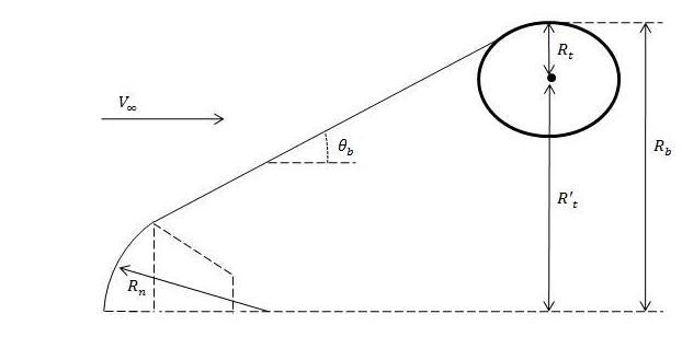
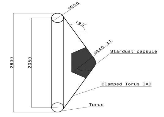
Following procedure was adopted for designing the IAD configuration, 1. As mentioned in the previous section, clamped torus IAD was selected for our study. Main geometrical parameters for a clamped torus IAD is shown in Figure 4.2. Entry capsule near the nose of IAD is taken as Stardust baseline configuration. 2. Ballistic coefficient, β of Stardust capsule with IAD was fixed to be 6kg/m2 . 3. Mass of the Stardust capsule with IAD was retained to be same as baseline Stardust capsule as 45.8kg. 4. Nose radius, included angle was also retained as 0.23m and 60ᴼ, same as baseline Stardustcapsule.

Fig 4.2: Toroidal ballute geometry definitions capsule [17]

5. a assumed initial CD of 1.4, the cross sectional area, S of IAD was computed from the following equation,

6.

7. From the value of S, the overall diameter of IAD, Rb was computed using equation, . Torus radius Rtwas assumed to be 125mm, and using the following equation [17] CD of the ballute was computed, Fig 4.3: Flowchart of the process

The Equation (4.3) given above can be broken down by the contribution of each of the three main geometric elements of the clamped torus ballute. The first term in equation (4.3) is the drag coefficient of the spherical nose portion (the Stardust capsule forebody), the second term is the drag of the ballute conical frustum, and the last terms comprise the drag from the exposed portion of the ballute torus itself. 1. The obtained CD was substituted back to equation 4.1 and the sameprocedure was repeated. 2. The iterations were continued until the difference of CD between subsequent iterations is nearly zero. 3. Figure 4.3 shows the flowchart for the above procedure. Following table-4.2 gives the IAD configuration parameters, Table 4.2:IAD design parameters

Sl Design parameter Value No

1 Ballistic coefficient, β 6 kg/m2 2 Included angle 60ᴼ 3 Coefficient of Drag, CD 1.435 4 5 Reference radius, Rb

Torus radius, Rt 1.3m 0.125m

4.5 Final IAD configuration

Figure 4.4 given below is the final IAD configuration that we generated by using the designed parameters.

© 2020, D m C S  4.1 2 bS R             2 2 2 24 2 , 2 2 3 4 2 ' cos 1 (sin ) 2(sin ) cos 4 2 3 cos cos sin 3 t t b n n D ballute b b b b b b t b t t b b b b b R R R R C R R R R R R R R R                                               4.3 IRJET |

International Research Journal of Engineering and Technology (IRJET) Volume: 07 Issue: 09 | Sep 2020 www.irjet.net e-ISSN: 2395-0056 p-ISSN: 2395-0072

Fig 4.4: Stardust with IAD

Reference area of the vehicle with IAD increased by 10.3 times than its actual reference area. The large reference area will result in higher drag and deceleration at higher altitudes.

5. HEAT FLUX ESTIMATION AND TPS DESIGN

In this chapter, the heat flux computation during reentry and TPS required for reentry will be discussed.

5.1 Convective Heating at stagnation point

Empirical correlation available in literature [23] for finding the convective heat flux generation during the earth reentry. The vehicle is entering from an altitude of 120km having a velocity of 8 km/s, Vehicle nose radii is 0. 23m. The updated convective heating correlations use a simple functional form and are split over two different shock speed regimes. The correlations have been validated for densities of (altitudes of approximately 83.5 to 38.5 km), and nose radii of 0.2 to 10 m For :[23]

(5.1)

For

(5.2)

Where is the convective heat flux in

is the density in V is the velocity in m/s and R is the nose radius in m. Our entry velocity is 8km/s. There for we are using the correlation (5.1) and with this correlation we are validating our flight data.

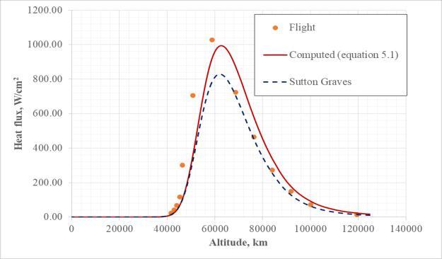
5.1.1 Heat flux validation

Figure 5.1 shows the heat flux as a function of altitude obtained using this correlation. Heat flux obtained using the empirical correlation shows a good comparison with the Stardust flight heat flux [23] and Sutton graves correlation heat flux. Fig 5.1: Heat flux Validation

5.2 Thermal Protection System (TPS) design for IAD

TPS for IAD is a flexible system designed to maintain structural component temperatures while surviving the thermal loads, mechanical shear and pressure environments during re-entry. TPS layups are made up of multiple layers of materials and fabrics which satisfy specific engineering functional aspects.

5.2.1 Overall configuration of TPS

In general, TPS configuration for IAD consists of three major layers. During reentry, outer fabrics experience shearing, pressure, and hot gas impingement resulting in high surface temperatures on the outer surface. Some critical aspects of the outer fabrics are •Strength of the material after packing and deployment •Permeability of the fabric which limits hot gas flow into the layup • Ability to withstand high temperatures as a result of convective heating Insulators are positioned behind the outer fabrics, and will experience a small amount of shearing flow, but are required to reduce temperatures from outer fabrics to below the maximum usable temperature limits of the structural components. Gas barrier materials are necessary to eliminate the potential for hot gas flow through the layup, but will not experience high temperatures, or shearing flow. The gas barrier layer will be attached directly to the structural components, so the gas barrier must be able to withstand a moderate level of heating.

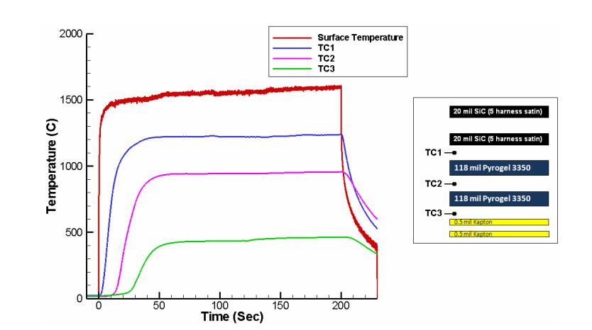
5.2 TPS selection criteria

TPS configuration was shown in figure 5.3 is selected based on literature survey. [26]The configuration was tested [26] in NASA Laser-Hardened Materials Evaluation Laboratory (LHMEL) facility at a heat flux of 50W/cm2 for 200s by exposing it to CO2 LASER. Fig 5.4 shows the test data from the LHMEL test for the TPS.

International Research Journal of Engineering and Technology (IRJET) Volume: 07 Issue: 09 | Sep 2020 www.irjet.net e-ISSN: 2395-0056 p-ISSN: 2395-0072

Fig 5.4: TPS test data in NASA LHMEL facility [26]

5.2.1 TPS design verification methodology

For verifying, whether the selected TPS will survive the reentry heating experience during by the IAD, following methodology was adopted, 1.Developing thermal model for the TPS in ANSYS software. 2.Fine tuning of thermal contact conductance between the TPS layers to match the test data shown in Fig 5.3. 3.Verify TPS performance for the actual re-entry heat flux experienced by IAD.

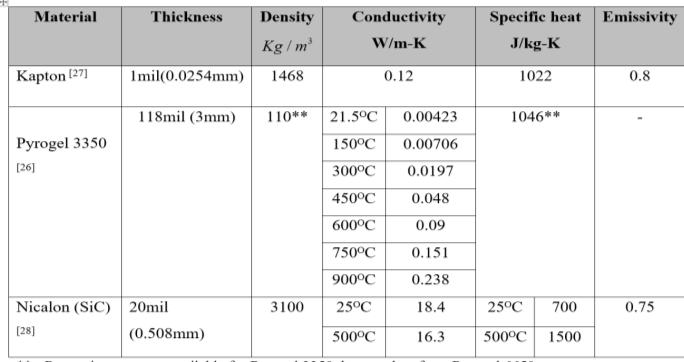
5.2.2 Thermo-physical properties

Thermo-physical properties for theTPS materials is given in figure 5.5

** -Properties were not available for Pyrogel 3350, hence taken from Pyrogel 6650 Fig 5.5 TPS Materials thermal physical properties

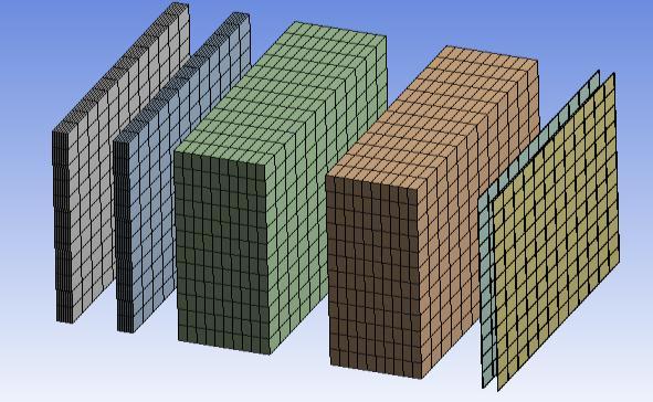
5.2.3Thermal model

One dimensional thermal model was generated for analysis. Thermal model, Boundary conditions and layup of TPS is shown in Fig 5.6. In general, inflatable torus is taken as structure. Fig 5.7 shows the meshed geometry of the TPS model. 5 nodes were given along thickness directions in all TPS materials including Kapton. Fig 5.61-D diffusion based thermal model concept

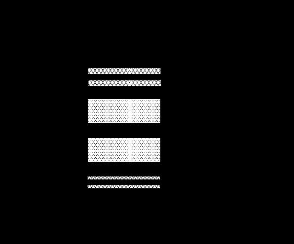
In this analysis data, structure was not considered.

Fig 5.7Meshed thermal model

5.2.7 Comparison with NASA LHMEL experimental data [26]

Thermal contact conductance between TPS was fine tuned to match the NASA LHMEL test data. Fine-tuned thermal contact conductance between adjacent layers are given in table 5.1

Table 5.1Thermal contact conductance Contact Surfaces Thermal contact conductance

Nicalon -Nicalon

Nicalon -Pyrogel Pyrogel-Pyrogel Pyrogel -Kpton Kapton -Kapton 100

100 30 200 1000

Fig 5.8shows the comparison of temperature history with NASA LHMEL experimental data.

International Research Journal of Engineering and Technology (IRJET) Volume: 07 Issue: 09 | Sep 2020 www.irjet.net e-ISSN: 2395-0056 p-ISSN: 2395-0072

Fig 5.8: Thermocouple temperature at various layers

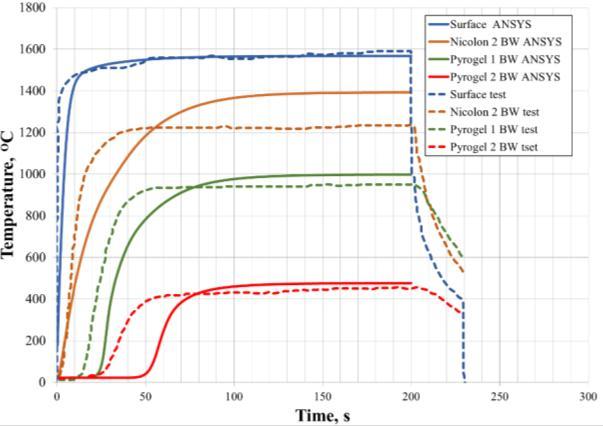
Though the initial transients could not be matched, the steady state temperatures are comparable in the surface and interlayers. Presently analysis was carried out with constant thermal contact conductance and with temperature dependent thermal contact conductance the transients can also be matched. Presently the high temperature properties are not available also the conductivity varies with respect to pressure is not available, therefore entire finding is based on thermal contact conductance. So, this is to be noted. Figure 5.8 shows the temperature contours obtained from ANSYS analysis for the comparison of NASA LHMEL experimental data. Fig 5.8: Temperature contour (ANSYS analysis comparison with NASA LHMEL experimental data) With the thermal contact conductance fine-tuned to match experimental data, the analysis will be repeated with the actual IAD re-entry heat flux on the same TPS configuration.

6. RESULT AND DISCUSSION

In this chapter, we present the result and discussion of our project as follows, 1. Trajectory, heat flux, dynamic pressure, deceleration loads, Mach number and Reynolds number comparison of Stardust LEO reentry with and without IAD. 2. TPS design for stardust LEO reentry. 6.1 Stardust LEO re-entry and Stardust LEO re-entry with IAD After validation of trajectory and heat flux estimation with Stardust flight data, the program was used for computing the trajectory for Stardust Low earth orbit reentry (LEO) with and without IAD attached.

Table 6.1 gives the parameters for trajectory design.

Sl Parameter Stardust LEO re- Stardust LEO No entry re-entry with IAD

1 Entry 120km 120km altitude 2 Entry 8km/s 8km/s velocity (Initial) 3 Ballistic 60kg/m2 6kg/m2 coefficient 4 Entry Flight -2ᴼ -2ᴼ path angle (EFPA) 5 Nose radius 0.23m 0.23m

6.1.1 Altitude Vs Velocity

Figure 6.1 gives the trajectory for Stardust LEO reentry with and without IAD.

From the trajectory it is evident that,

1.Much of the deceleration for Stardust with IAD happens at

high altitudefrom 100 to 50km where density is low. Fig 6.1: Altitude Vs Velocity

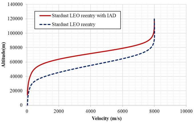
2. For stardust without IAD, the deceleration happens at relatively lower altitudes from 80 to 30km. 3.This deceleration at higher altitude has a direct influence on the reentry loads such as heta flux, dynamic pressure etc. These will be explained in subsequent sections.

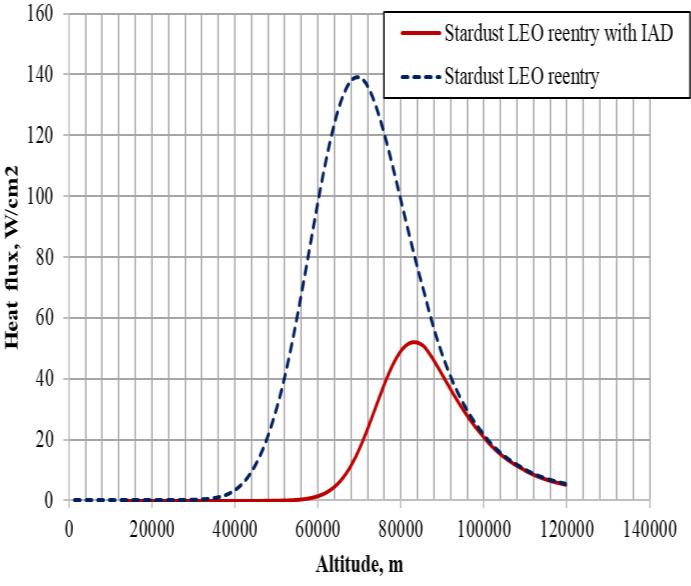
6.1.2 Heat Flux

Figure 6.2 gives the comparison of heat flux estimated at stagnation point as a function of altitude for Stardust LEO reentry with and without IAD.

From the estimated heat flux, it is evident that,

International Research Journal of Engineering and Technology (IRJET) Volume: 07 Issue: 09 | Sep 2020 www.irjet.net

1.Peak heat flux for Stardust LEO reentry is 140W/cm2 at 70km and for Stardust LEO reentry with IAD it is 51.2W/cm2 at 84km. 2.Lowering of ballistic coefficient from 60kg/m2 to 6kg/m2 with attachment of IAD has resulted in a 63% reduction on the reentry peak heat flux. 3.This lower heat flux will have a direct influence on the TPS design, as lightweight TPS can be used for the reentry capsule.

e-ISSN: 2395-0056 p-ISSN: 2395-0072

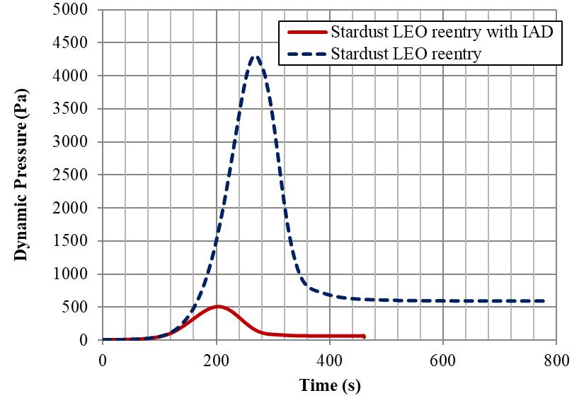
Fig 6.2: Heat Flux vs Altitude

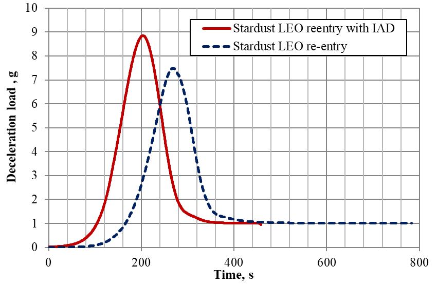
6.1.3 Deceleration Load

Figure 6.3, gives the comparison of deceleration load history for Stardust LEO reentry with and without IAD. Fig 6.3: Deceleration load history From the estimated deceleration load history, it is evident that, 1.Peak deceleration load for Stardust LEO reentry is 7.5g’s and for Stardust LEO reentry with IAD it is 8.9g’s. 2.There is a marginal increase (18.6%) in deceleration load which is anticipated, as the large drag area of the IAD causes a larger deceleration.

6.1.4 Dynamic pressure

Figure 6.4 gives the comparison of dynamic pressure history for Stardust LEO reentry with and without IAD. Fig 6.4: Dynamic Pressure history

From the estimated dynamic pressure history, it is evident that, 1.Peak dynamic pressure for Stardust LEO reentry is 43. kPa and for Stardust LEO reentry with IAD it is 0.5kPa. 2.There is a drastic reduction (98%) in dynamic pressure with the IAD attached to the stardust capsule. 3.Dynamic pressure is a function of density and velocity, the very low velocity at denser lower altitude for stardust with IAD has resulted in this lower dynamic pressure.

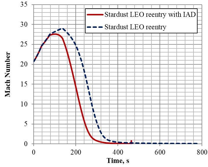
6.1.5 Mach number

Figure 6.5 shows the Mach number history for Stardust LEO reentry with and without IAD. Mach number is slightly higher in case of Stardust LEO re-entry without IAD, as it

travels at a higher velocity in the lower atmosphere. Fig: 6.5: Mach number history

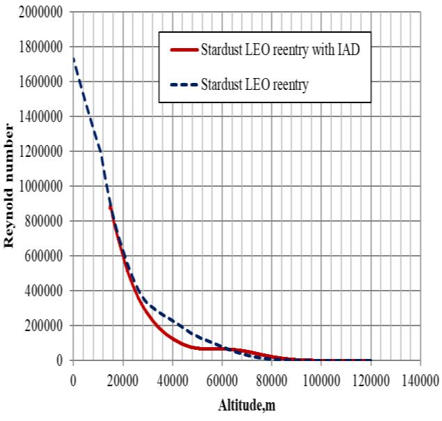
6.1.6 Reynolds number

For calculating Reynolds number, we are taking density and temperature directly from the atmospheric model and dynamic viscosity is calculated using the equation given below.

Where and x are constant values ( , x = 110.4)In case of stardust LEO re-entry vehicle, the overall

International Research Journal of Engineering and Technology (IRJET) Volume: 07 Issue: 09 | Sep 2020 www.irjet.net e-ISSN: 2395-0056 p-ISSN: 2395-0072

diameter is taken as 2.6 meter and in the case of stardust LEO re-entry with IAD the overall diameter is 6.128m. Figure 6.6 shows the Reynolds number history for Stardust LEO reentry with and without IAD. Though Re is nearly similar for both cases, a slightly lower Re is observed for Stardust LEO reentry with IAD.

Fig 6.6: Reynolds Number vs Altitude

6.2 Thermal response of TPS

From the table given above, we can calculate the total aerial weight of our TPS by adding the twice of each material aerial weight. Now we get a value of

Table 6. 1: Flexible TPS material thickness and aerial weight Material Thickness Areal weight Cm (g/cm²) Nicalon (5 Harness Satin 0.0506 0.0425 (26x26)) Pyrogel 3350 0.3047 0.0518 Kapton 0.0025 0.0037

Fig 6.7 shows the thermal response of the TPS interlayers for the IAD re-entry heat flux given in Figure 6.2.

Fig 6.7: Thermocouple temperatures at various layers [26]

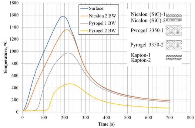
The peak surface temperature is nearly 1600ᴼC, which is well within the continuous operating temperature of Nicalon, which is 1800ᴼC. The Pyrogel-1 temperature and Kapton-1 temperature has exceeded their respective temperature constraints of 1100ᴼC and 400ᴼC. But the material remains at the peak temperature only for a very short duration. With the introduction of an additional Nicalon and Pyrogel layer, the temperature can be further reduced.

CONCLUSION OF THE PROJECT

Thermal protection system design to survive the reentry heat flux with a low ballistic coefficient Inflatable Aerodynamic Decelerator (IAD) for ballistic reentry from Low Earth Orbit (LEO) was carried out.For this, a ballistic entry trajectory design program was developed with an inbuilt atmospheric model and gravity model and was validated with stardust flight data. As baseline, Stardust entry probe configuration from LEO entry was selected. Suitable IAD was configured, which was attached to the Stardust entry probe to reduce the ballistic coefficient from 60kg/m2to 6kg/m2. Trajectory, heat flux, dynamic pressure and deceleration loads were compared for Stardust entry probe with and without IAD attached. From the trajectory, the heat flux on the IAD was estimated using empirical correlation. Flexible thermal protection system capable of surviving the re-entry heat flux was selected based on literature survey. A thermal model was developed in ANSYS and the thermal contact conductance between the TPS interlayers were fine-tuned with experimental data. With the fine-tuned thermal contact conductance analysis was carried out with the IAD reentry heat flux. The selected thermal protection system consisting of 2 Nicalon (SiC) layers as the outer layer followed by two Pyrogel 3350 layer as insulator and 2 Kapton layers as gas barrier is capable of surviving the re-entry heating. For our TPS the aerial density is The temperature can be bringing down with in a limited value while applying additional layer.

REFERENCES

1. Henry Wright et al., “HEART flight test overview”, 9th International Planetary Probe Workshop, 16-22 June 2012, Toulouse. 2.“Integrated design for space transportation system”,B N Sivan ,Springer eBook,ISBN 978-81-3-53-4 3.https://en.wikipedia.org/wiki/Project_Mercury 4.https://en.wikipedia.org/wiki/Space_Capsule_Recovery_E xperiment 5.https://en.wikipedia.org/wiki/Stardust_(spacecraft) 6.https://en.wikipedia.org/wiki/Genesis_(spacecraft) 7.https://en.wikipedia.org/wiki/Apollo_(spacecraft) 8.https://en.wikipedia.org/wiki/Soyuz_(spacecraft) 9.https://en.wikipedia.org/wiki/Shenzhou_program 10.https://en.wikipedia.org/wiki/Space_Shuttle 11. Header, D.R. “A Miniature Version of the JA70 Aerodynamic Heating Computer Program, H800 (MINIVER),"