3.1 LeNet

International Research Journal of Engineering and Technology (IRJET) e-ISSN: 2395-0056 Volume: 07 Issue: 08 | Aug 2020 www.irjet.net p-ISSN: 2395-0072

better training speed.It also has Batch Normalization but present only on the top of traditional layer not on summations.They have a set of filters with sizes 1x1,3x3, 5x5, etc.that are merged with concatenation in each branch. Each Inception block is connected with a filter expansion layer of size 1x1 which is used for scaling up the dimensions of the filter bank before the addition . This model includes Inception ResNet-A,Inception ResNet-B,Inception ResNetC[29].

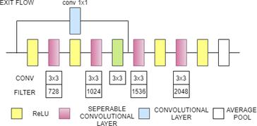
Fig. 7(a). InceptionResNetV2 Architecture

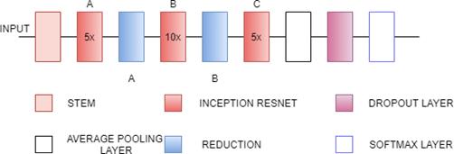
Fig. 7(b). InceptionResNetV2 Architecturedetailed

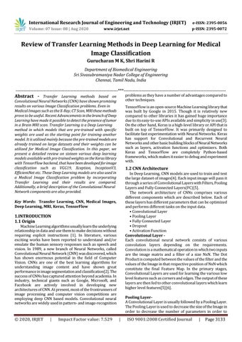
3.8 Xception

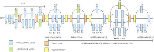
Xception stands for Extreme Inception and it is 71 layers deep. Xception was developed by Francois Chollet, the creator and chief maintainer of the Keras library. Xception contains modified inception block whixh is wide and replaced the different spatial dimensions such as 1x1, 5x5, 3x3 with a single dimension (3x3) followed by a 1x1 convolution to regulate computational complexity. The Xception model is based on inception module with modifications in convolutional and depthwise separable convolution layers.It has three major blocks: Entry Flow, Middle Flow, and Exit Flow. It has 36 convolutional layers. These layers are structured into 14 modules, Except the first and last module,all these modules have linear residual connectiona around them. The data first enters the entry flow, then goes through the middle flow which is repeated eight times, and finally through the exit flow. All Convolution and depthwise separable Convolution layers are followed by batch normalization[30]. Fig. 8(b). Xception Architecture(Entry flow)

Fig. 8(a). Xception Architecture

Fig. 8(c). Xception Architecture(Middle and exit flow)

3.9 DenseNet121

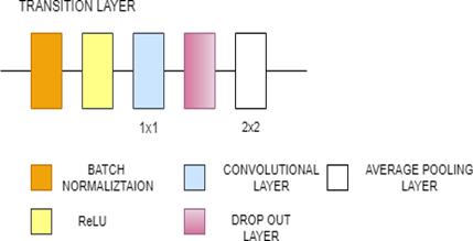
DenseNet121 is 121 layers deep, densely connected convolutional network. There are three Sections in the DenseNet121 architecture. The first is convolution block, which is a basic block in the DenseNet architecture. Convolution block in DenseNet is similar to the identity block in ResNet. The second section is the dense block, in which the convolution blocks are concatenated and densely connected. Dense block is the main block in DenseNet architecture[27]. The last is the transition layer, which connects two contiguous dense blocks. The size of the feature maps are the same in the dense block. Transition block reduces the dimension of feature maps. It has approximately 8M parameters.[31]

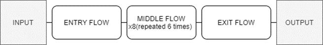
Fig. 9(a). DenseNet121 Architecture

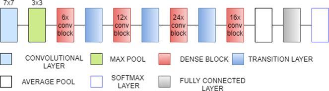
Fig. 9(b). DenseNet121 Architecture(Dense block and transition layer)

3.10 DenseNet169

DenseNet169 is 169 layers deep, densely connected convolutional network. There are three Sections in the DenseNet169 architecture. The first is convolution block, which is a basic block in the DenseNet architecture. Convolution block in DenseNet is similar to the identity block in ResNet. The second section is the dense block, in which the convolution blocks are concatenated and densely connected. Dense block is the main block in DenseNet architecture. The last is the transition layer, which connects

International Research Journal of Engineering and Technology (IRJET) e-ISSN: 2395-0056 Volume: 07 Issue: 08 | Aug 2020 www.irjet.net p-ISSN: 2395-0072

two contiguous dense blocks. The size of the feature maps are the same in the dense block. Transition block reduces the dimension of feature maps. It has approximately 14.3M parameters[31].

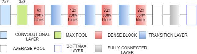
Fig. 10. DenseNet169 Architecture

3.11 DenseNet201

DenseNet201 is 201 layers deep, densely connected convolutional network. There are three Sections in the DenseNet201 architecture. The first is convolution block, which is a basic block in the DenseNet architecture. Convolution block in Densenet is similar to the identity block in ResNet. The second section is the dense block, in which the convolution blocks are concatenated and densely connected. Dense block is the main block in DenseNet architecture. The last is the transition layer, which connects two contiguous dense blocks. The size of the feature maps are the same in the dense block. Transition block reduces the dimension of feature maps. It has approximately 20.2M parameters[31].

3.12 MobileNetV2

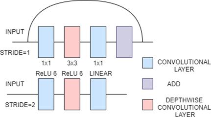
MobileNetV2 is based on an inverted residual structure and a linear bottleneck layer[32]. There are two types of blocks in MobileNetV2. One is the residual block with stride of 1. Another one is the residual block with stride of 2 for downsizing with each block having three layers. First layer is a 1x1 convolutional layer with ReLU6 [32]. The second layer is the depth wise convolution which uses 3x3 depth-wise separable convolution and the third layer is linear 1x1 convolutional layer. It has 3.4M parameters[33].

3.13 NasNetMobile and NasNetLarge

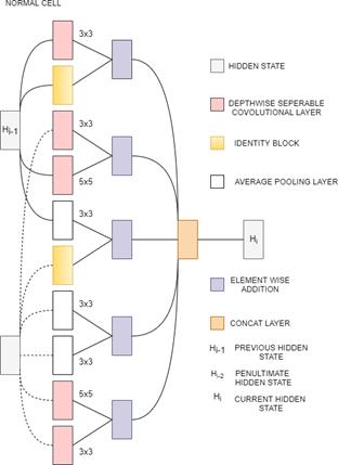
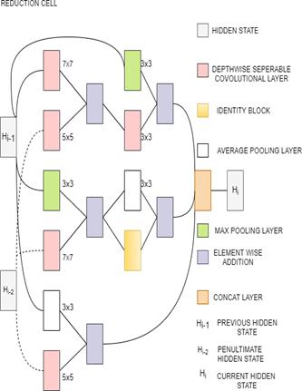
NasNetMobile is a Scalable Convolutional Neural Network. It consists of a few basic building blocks. Each block consists of a few basic operations that are repeated multiple times according to the required capacity of the network. It has 12 blocks and about 5.3M parameters. The default input size is 224x224. Block is the smallest unit in NASNet. Cell is a combination of blocks[34][33]. NasNetLarge is a convolutional neural network that is trained on more than a million images from the ImageNet database which has over 88M parameters. It consists of two repeated motifs termed as Normal cell and Reduction cell[35]. In normal cells, convolutional cells return a feature map of the same dimension. In reduction cells, convolutional cells return a feature map with the dimensions reduced by a factor of 2[36]. NAS-Neural Network Search is an algorithm that is used to search for the best neural network architecture[37].In the NAS algorithm, controller Recurrent Neural Network (RNN) samples the blocks and puts them together to create end-to-end architecture. The default input

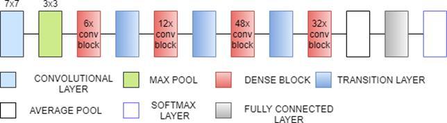
Fig. 13(a). NasNet Architecture

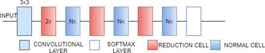
Fig. 11. DenseNet201 Architecture

size is 331x331.

Fig. 12. MobileNetV2 Architecture

Fig. 13(b). NasNet Architecture(Normal and Reduction cell)

3.14 EfficientNetB0

The EfficientNet group consists of 8 models from B0 to B7. In this model a new scaling method called” Compound Scaling” was introduced. Compound scaling method uses a compound co-efficient to uniformly scale all the three dimensions( depth,width, and resolution) together. This new family of models was created using the NAS (Neural Architecture Search) algorithm[37]. This NAS Algorithm is used to find the optimum baseline network. In all the 8 models, the first (stem) and final layers are common. After this, each model consists of seven blocks. These blocks have varying numbers of sub-blocks whose number is increased as we move from

International Research Journal of Engineering and Technology (IRJET) e-ISSN: 2395-0056 Volume: 07 Issue: 08 | Aug 2020 www.irjet.net p-ISSN: 2395-0072

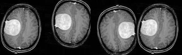
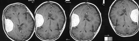
EfficientNetB0 to EfficientNetB7. EfficientNetB0 has approximately 5.3M trainable parameters[38]. layer) In our experiments, we evaluate the performance of our CNN transfer learning models on a Medical Image Classification to detect the presence of Tumor in a Brain MRI. The original dataset of MRI Images consisted of a total of 253 images with 153 images with Tumor labelled as ‘yes’ and 98 images without Tumor labelled as ‘no’. These images are obtained from Brain MRI images for tumor detection dataset by Navoneel Chakrabarty[39]. The dataset was built by experienced radiologists using real patient’s data. All the images are resized to 150X150. Figure 15(a) and 15(b) show the MRI Images with tumor and without tumor respectively.

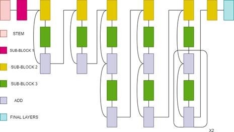
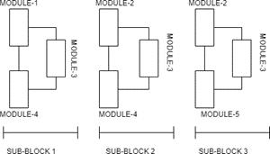
Fig. 14(a). EfficientNetB0 Architecture

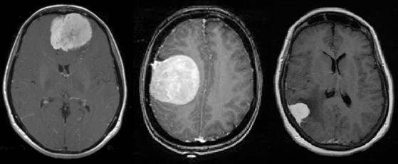
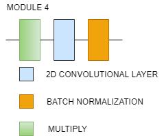
Fig. 14(b). EfficientNetB0 Architecture(Stem and module)

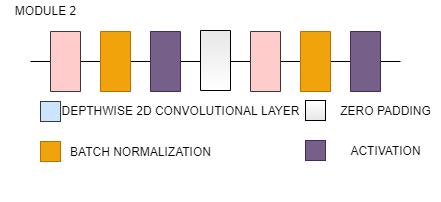
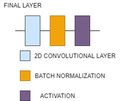
Fig. 14(c). EfficientNetB0 Architecture(Modules and Final

4. METHODOLOGY 4.1 Data Pre-processing –

Fig. 15(a). With Tumor Fig. 15(b). WithoutTumor

4.2 Data Augmentation–

Data Augmentation is a technique in which the size of the training dataset is artificially expanded by creating modified versions of images in the dataset which will enhance the capability of the model to learn and generalize better on future unseen data[40]. In order to account for the data imbalance and more numberof images, these images were augmented to get a total of 1085 images with Tumor and 979 images without Tumor. Figure 16(a) and 16(b) show the ways in which an image is augmented to account for more number of data. Table 1 gives the details of the dataset before and after data augmentation. Table 1. Data Analysis Original Dataset Tumor (Total- After Data S.no. Class 253) Augmentation NumberPercentageNumber Percentage 1 Yes 155 61.26 1085 52.57 2 No 93 38.74 979 47.43 Total 253 100 2064 100

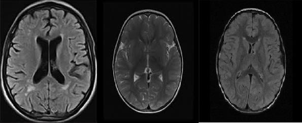
Fig. 16(a). Data Augmentation

International Research Journal of Engineering and Technology (IRJET) e-ISSN: 2395-0056 Volume: 07 Issue: 08 | Aug 2020 www.irjet.net p-ISSN: 2395-0072

Fig. 16(b). Data Augmentation

4.3 Data Splitting –

After the data has been augmented as per the requirement, the data is then split into the training set and the test set. In this experiment, the Test-Train ratio has been set at 0.2 indicating that 80% (1651 images) of the images will go to the training set which will be used by the neural network to get trained and the remaining 20% (413 images) of the images will go to the test set on which the trained neural network will be applied and to check the validation (test) accuracy of the Neural Network. Table 2 gives the number of images split to the training and the test set. Table 2. Data Splitting Test-Train Brain MRI Split Ratio: S.no. Tumor 0.2 Number Percentage 1 Training set 1651 80 2 Test set 413 20 Total 2064 100

4.4 CNN Architectures –

Transfer learning is a technique in which a pre-trained model is taken that has already been trained on a related task of Image Classification and reusing the weights in the new model to be trained in this experiment. The CNN Architectures on which fine tuning of parameters is performed to apply Transfer Learning are given in Table 3. Table 3. Pre-Trained Models

Year Architecture Published Number of Parameters Name

LeNet-5 1998 0.060 M AlexNet 2012 60 M VGG16 2014 138.3 M VGG19 2014 143.6 M ResNet-50 2015 25.6 M InceptionV3 2015 23.8 M InceptionResNet 2016 55.8 M

V2

ResNet152V2 2016 60.3 M Xception 2016 22.9M DenseNet121 2017 8 M DenseNet169 2017 14.3 M DenseNet201 2017 20.2 M MobileNetV2 2018 3.5 M NasNetMobile 2018 5.3 M NasNetLarge 2018 88.9 M EfficientNetB0 2019 5.3 M For this experiment, we decided to keep all the major parameters such as the optimizer, loss function constant for all the CNN Architectures so that the results can be compared on equal grounds. The following are the hyperparameters that have been used to train all the Transfer Learning models used in this Brain MRI Tumor Image Classification. Weights:imagenet Optimizer: SDG (Stochastic Gradient Descent) with Learning Rate of 0.001 Loss Function: Binary Cross Entropy Metrics: “acc”

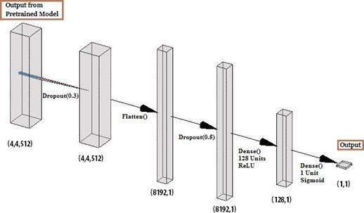
4.5 Layers Used–

1. Output Layer of the Pre-trained Model (VGG19,

InceptionV3 etc.) 2. Dropout Layer with probability of 0.3 3. Flatten Layer 4. Dropout Layer with probability 0.5 5. Dense Layer with 128 units and ReLU activation function 6. Dense Layer with 1 unit and Sigmoid activation function

4.4 Training and Validation Generator details -

Image Size: (150,150,3) * Batch size: 64 Class Mode:Binary Number of Epochs:30 * NasNetMobile required an image size of (227,227,3) and NasNetLarge required an image size of (331,331,3)

4.7 Transfer Learning Model Architecture

Fig. 17. Transfer Learning Model Architecture

5. RESULTS

These pre-trained models were used to classify the Brain MRI images to detect the presence of tumor in it. All the models were trained for 30 epochs and the results are tabulated below in Table 4.

International Research Journal of Engineering and Technology (IRJET) e-ISSN: 2395-0056 Volume: 07 Issue: 08 | Aug 2020 www.irjet.net p-ISSN: 2395-0072

Table 4. Results

Validation Training Accuracy Validation AccuracyTraining CNN Architecture(%) Loss (%) Loss

DenseNet121 94.18 0.19 96.42 0.08 InceptionV3 92.73 0.28 98.18 0.04 Xception 92.73 0.29 98.84 0.03 ResNet152V2 91.76 0.36 99.33 0.02 NasNetMobile 91.28 0.49 99.15 0.02 VGG19 90.55 0.24 86.73 0.3 DenseNet201 90.55 0.37 99.03 0.02 MobileNetV2 90.31 0.4 99.45 0.02 NasNetLarge 90.31 0.49 100 0 DenseNet169 89.83 0.47 97.81 0.05 InceptionResNetV87.89 0.35 96.97 0.07

2

AlexNet 87.89 0.42 82.98 0.38 VGG16 87.16 0.31 87.4 0.28 ResNet-50 77.23 0.52 68.07 0.59 LeNet-5 72.88 0.43 86.67 0.31 EfficientNetB0 52.3 1.3 89.7 0.24

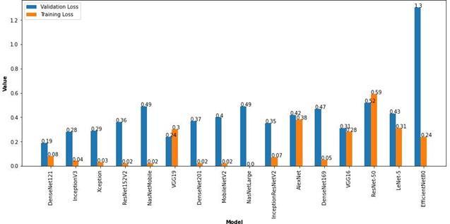
From the above tabulated results, it can be seen that the DenseNet121 with 8M parameters has the highest validation accuracy of 94.18% among all the other models that were built with the same hyperparameters and trained on the same Medical Image dataset of Brain MRI Scan images. InceptionV3 and Xception models also show accuracies of 92.73% on the validation set but the higher training accuracies denote that there is a tendency towards over fitting. The ResNet152V2 and NasNetMobile show validation accuracies of 91.76% and 91.28% respectively. The training accuracies of above 99% in both the models also denotes the possibility of overfitting. The VGG19 and DenseNet201 architectures have an accuracy of 90.55% on the validation set but the training set accuracy of the VGG19 architecture is 86.73% which denotes that more training is required to achieve higher accuracy. On the other hand, DenseNet201 has the training accuracy of 99.03% which shows overfitting. The MobileNetV2 and NasNetLarge architectures have validation accuracies of 90.31% and have high training accuracies of 99.45% and 100% respectively. This clearly denotes that the model has over fit the training data and can be rectified by fine-tuning the hyperparameters. The DenseNet169 and InceptionResNetV2 architectures have shown a validation accuracy of 89.83 and 87.89 respectively which can also be improved by fine tuning the hyperparameters. The AlexNet architecture with over 60M parameters is one of the old architectures developed which performed well with a validation accuracy of 87.89% and training accuracy of 82.98%. The VGG16 model also gave a validation accuracy of 87.16% which can be improved by fine-tuning the hyperparameters. The ResNet-50 model showed a very poor training accuracy of 68.07% and hence produced a lower validation accuracy of 77.23%. This means that the hyperparameters need to be fine-tuned to improve the trainingaccuracy which will improve the validation set accuracy. The LeNet-5 Architecture which was developed in 1998 managed to give a validation accuracy of 72.88% and a training accuracy of 86.67%. Though this model’s architecture has a very low number of parameters, it managed to learn the features of the training classes to produce reasonable accuracies. The latest EfficientNetB0, which was published in 2019 failed to achieve a good validation accuracy and suffered from heavy overfitting on training with the above mentioned hyperparameters. The validation accuracy remained very low at 52.30% while the training accuracy was 89.70%. This can be corrected by adjusting the hyperparameters to prevent overfitting. The results of these pre-trained models with transfer learning are available at https://github.com/mkgurucharan/Transfer-Learning-Methodsfor reference. The Bar plot of the accuracies and losses of the various CNN architectures areshown in Figure 18 and 19 respectively.

Fig 18. Accuracy Bar Plot

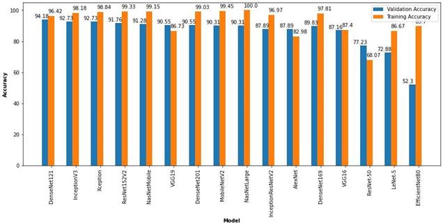
Fig. 19. Loss Bar Plot

6. CONCLUSION AND FUTURE SCOPE

In this paper, sixteen pre-trained CNN models have been built using Transfer Learning and have been used to classify the Brain MRI Images if they have a Tumor or not. The Data is pre-processed with a standard size and augmented to increase the size of the training set to prevent overfitting. Among all the models, keeping the various hyperparameters such as optimizer and loss function constant, DenseNet121 showed the highest validation accuracy of 94.18% with the lowest validation loss of 0.19. The other models such as

International Research Journal of Engineering and Technology (IRJET) e-ISSN: 2395-0056 Volume: 07 Issue: 08 | Aug 2020 www.irjet.net p-ISSN: 2395-0072

Xception, InceptionV3 and ResNet50 also performed well with accuracies higher than 90%. Some of the models such as NasNetLarge and EfficientNetB0 suffered from overfitting. From these results, the pre-trained models that can be used by implementing Transfer Learning for Medical Image Classification on a small number of images can be comprehended. The future possibility could be to use a larger dataset to control the occurrence of overfitting. Additionally, extensive tuning of the hyperparameters such as optimizer and loss on the models can be performed to result in a high accuracy for Medical Image Classification with Deep Learning.

5. REFERENCES

[1] J. G. Carbonell, “Machine learning research,” ACM SIGART Bull., vol. 18, no. 77, pp. 29–29, 1981, doi: 10.1145/1056743.1056744. [2] N. Jmour, S. Zayen, and A. Abdelkrim, “Convolutional neural networks for image classification,” in 2018 International Conference on Advanced Systems and Electric Technologies (IC_ASET), 2018, pp. 397–402, doi: 10.1109/ASET.2018.8379889. [3] M. Abadi et al., “TensorFlow: Large-Scale Machine Learning on Heterogeneous Distributed Systems,” 2016, [Online]. Available: http://arxiv.org/abs/1603.04467. [4] T. Zhou, S. Ruan, and S. Canu, “A review: Deep learning for medical image segmentation using multimodality fusion,” Array, vol. 3–4, no. August, p. 100004, 2019, doi: 10.1016/j.array.2019.100004. [5] A. Khan, A. Sohail, U. Zahoora, and A. S. Qureshi, “A survey of the recent architectures of deep convolutional neural networks,” Artif. Intell. Rev., pp. 1–70, 2020, doi: 10.1007/s10462-020-09825-6. [6] M. A. Wani, F. A. Bhat, S. Afzal, and A. I. Khan, “Basics of Supervised Deep Learning,” pp. 13–29, 2020, doi: 10.1007/978-981-13-6794-6_2. [7] Y. Zhu et al., “Heterogeneous transfer learning for image classification,” 2011. [8] M. Lagunas and E. Garces, “Transfer Learning for Illustration Classification,” 2018, doi: 10.2312/ceig.20171213. [9] K. E. Emblem et al., “Predictive modeling in glioma grading from MR perfusion images using support vector machines.,” Magn. Reson. Med., vol. 60, no. 4, pp. 945–952, Oct. 2008, doi: 10.1002/mrm.21736. [10] M. M. Beno, V. I. R, S. S. M, and B. R. Rajakumar, “Threshold prediction for segmenting tumour from brain MRI scans,” Int. J. Imaging Syst. Technol., vol. 24, no. 2, pp. 129–137, Jun. 2014, doi: 10.1002/ima.22087. [11] E. A. S. El-Dahshan, H. M. Mohsen, K. Revett, and A. B. M. Salem, “Computer-aided diagnosis of human brain tumor through MRI: A survey and a new algorithm,” Expert Syst. Appl., vol. 41, no. 11, pp. 5526–5545, 2014, doi: 10.1016/j.eswa.2014.01.021. [12] M. Rahmani and G. Akbarizadeh, “Unsupervised feature learning based on sparse coding and spectral clustering for segmentation of synthetic aperture radar images,” IET Comput. Vis., vol. 9, no. 5, pp. 629–638, 2015, doi: 10.1049/iet-cvi.2014.0295. [13] M. Lai, “Deep Learning for Medical Image Segmentation,” 2015, [Online]. Available: http://arxiv.org/abs/1505.02000. [14] O. Ronneberger, P. Fischer, and T. Brox, “U-net: Convolutional networks for biomedical image segmentation,” Lect. Notes Comput. Sci. (including Subser. Lect. Notes Artif. Intell. Lect. Notes Bioinformatics), vol. 9351, pp. 234–241, 2015, doi: 10.1007/978-3-319-245744_28. [15] Ö. Çiçek, A. Abdulkadir, S. S. Lienkamp, T. Brox, and O. Ronneberger,“3D U-net: Learning dense volumetric segmentation from sparse annotation,” Lect. Notes Comput. Sci. (including Subser. Lect. Notes Artif. Intell. Lect. Notes Bioinformatics), vol. 9901 LNCS, no. June 2016, pp. 424–432, 2016, doi: 10.1007/978-3-319-46723-8_49. [16] P. D. Chang, “Fully Convolutional Deep Residual Neural Networks for Brain Tumor Segmentation,” in Brainlesion: Glioma, Multiple Sclerosis, Stroke and Traumatic Brain Injuries, 2016, pp. 108–118. [17] S. Pereira, A. Pinto, V. Alves, and C. A. Silva, “Brain Tumor Segmentation Using Convolutional Neural Networks in MRI Images,” IEEE Trans. Med. Imaging, vol. 35, no. 5, pp. 1240–1251, 2016, doi: 10.1109/TMI.2016.2538465. [18] S. Iqbal, M. U. Ghani, T. Saba, and A. Rehman, “Brain tumor segmentation in multi-spectral MRI using convolutional neural networks (CNN),” Microsc. Res. Tech., vol. 81, no. 4, pp. 419–427, Apr. 2018, doi: 10.1002/jemt.22994. [19] P. Saxena, A. Maheshwari, S. Tayal, and S. Maheshwari, “Predictive modeling of brain tumor: A Deep learning approach,” 2019, [Online]. Available: http://arxiv.org/abs/1911.02265. [20] Y. Lecun, L. Bottou, Y. Bengio, and P. Ha, “LeNet,” Proc. IEEE, no. November, pp. 1–46, 1998, doi: 10.1109/5.726791. [21] A. El-Sawy, H. EL-Bakry, and M. Loey, “CNN for Handwritten Arabic Digits Recognition Based on LeNet-5BT -Proceedings of the International Conference on Advanced Intelligent Systems and Informatics 2016,” 2017, pp. 566–575. [22] A. Krizhevsky, I. Sutskever, and G. E. Hinton, “ImageNet Classification with Deep Convolutional Neural Networks,” Handb. Approx. Algorithms Metaheuristics, pp. 1–1432, 2007, doi: 10.1201/9781420010749. [23] K. Simonyan and A. Zisserman, “Very deep convolutional networks for large-scale image recognition,” 3rd Int. Conf. Learn. Represent. ICLR 2015 - Conf. Track Proc., pp. 1–14, 2015. [24] K. He, X. Zhang, S. Ren, and J. Sun, “Deep residual learning for image recognition,” Proc. IEEE Comput. Soc. Conf. Comput. Vis. Pattern Recognit., vol. 2016-Decem, pp. 770–778, 2016, doi: 10.1109/CVPR.2016.90. [25] M. Mateen, J. Wen, Nasrullah, S.Song, and Z. Huang, “Fundus image classification using VGG-19 architecture with