See It. Control It. Defining the Environment Before Deploying a Filtration Solution

By Jürgen M. Lobert, Director of AMC Technology, Entegris, Inc.

Many filtration solutions are deployed without accurately knowing the contamination challenges of the environment to be protected, either because no measurement has been done at all, or only qualitative evaluation methods like corrosion strips or generic particle estimates were used to define the state of contamination. In addition, many filter providers prefer to offer a few off the shelf products, rather than customizing the solution, in order to keep inventory and lead times low.

However, with sustainability becoming a strategic goal for most industrial operations, filter lifetime, cost of ownership and minimized waste streams are turning center stage of procurement and installation services. More importantly, processes, products and humans need to be better protected from contamination impact. Just like one would never use a simple MERV filter for a process needing ULPA filtration, one should not use a basic, off the shelf chemical filter with unknown capacity and removal efficiency for gas-phase contaminants.

Filter performance, as well as lifetime, can be optimized with the “See it. Control it.” paradigm, which is the most scientific, data-driven way to air filtration.

“The See It. Control It.” Paradigm

A proactive approach for contaminant removal is to choose the best filtration solution. Rather than using off the shelf products that might be cheaply and quickly available, the paradigm suggests to define the contamination first by characterizing the environment to be protected, and then finding or creating the most suitable solution for that specific environment.

The most important aspect of controlling gas-phase, airborne molecular contamination (AMC) and implementing filters is to define the contamination state of the environment to be protected. “The See it. Control it.” approach suggests to see the contamination through air analysis by a capable laboratory, which provides accurate gas phase analysis for any environment from the parts per million (ppm, 10-6) to the parts per trillion (ppt, 10-12) level.

The user can then control the environmental contamination more easily, as the filtration solution can be tailored exactly to that environment’s challenges and needs, as defined by the measurements. Some environments have an unusual mix of AMC classes and to prevent one portion of the filter being used up faster than others, filter vendors need to adjusts adsorbent mixes such that all adsorbents last about the same amount of time, based on the measurements of AMC in that environment.

What Is the Inkjet Cartridge Effect?

The idea of this approach is to avoid what we call the “inkjet cartridge effect,” referring to old style inkjet cartridges that held three equal amounts of magenta, yellow and cyan inks, but typically drained cyan first, forcing to discard a significant amount of yellow and magenta inks when replacing the cartridge. Applying our approach to this, we would determine first how much cyan, magenta and yellow is typically used up in a given amount of time, and then adjust the ink amounts accordingly such that all three are used up at about the same time (Figure 1).

 Figure 1: The inkjet cartridge effect for AMC filters visualized. The bars indicate filter lifetime in months for the respective contaminant classes (example: acids, bases, organics), the relative adsorbent (“ink”) amounts are indicated as numbers above each bar. Equal adsorbent amounts yield different lifetimes. Unified lifetime is achieved by using different adsorbent amounts.

For real-world filter scenarios, commercial environments usually attempt to remove acidic, basic and organic contaminants from air streams. Each of those classes has their own adsorbent for optimized removal but each also has different concentrations in any environment.

The most common and economical filter type for these applications is the combined adsorbent filter, which contains a mix of all adsorbents in one set of (usually pleated, V-bank or loose fill) media. Adjusting adsorbent amounts for an equalized lifetime of all contaminant classes is easy, if the measurements are available. However, each contaminant class may also have different priorities or importance for the application and in some cases, lifetimes may become secondary to the priority of removing one contaminant class more efficiently.

For particulate contamination, one should not only determine the overall particle count, but also the size distribution to determine impact on the process. Larger particles are easy to remove with low rating MERV filters, but more advanced processes might need HEPA and ULPA filters for best protection. Even those might still leave large numbers of very fine particles in the nanometer range to impact high technology processes. An understanding of these dependencies is important to define the best solution.

Filter Performance of Gas-Phase Filters

For gas-phase, chemical filters, the most critical performance characteristics are removal efficiency (RE) and capacity or remaining lifetime, but also pressure drop. Removal efficiency is defined as:

RE = (1 –Downstream) x 100(%) Upstream

With “Downstream” and “Upstream” being the contaminant concentrations up and downstream of the filter. Removal efficiency can be tracked over time to determine a practical end of filter life.

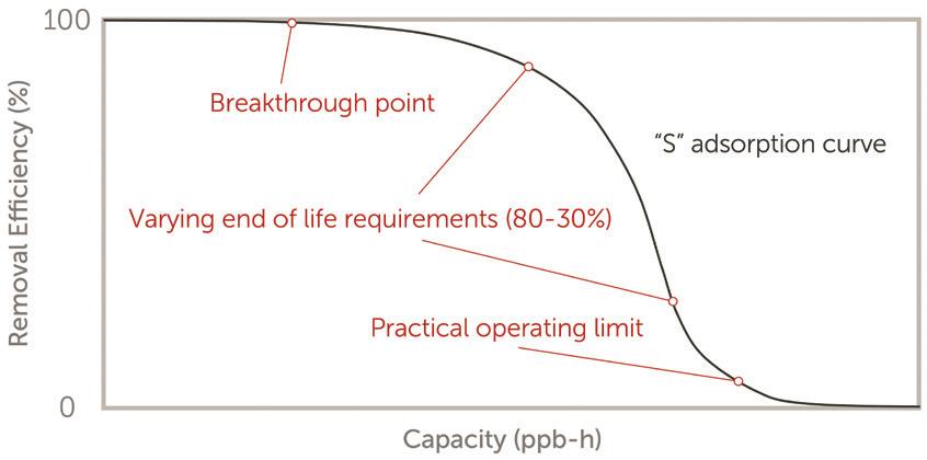
For AMC filters, removal efficiency is highest in the beginning and then decreases over time. Pressure drop does not appreciably change over time (AMC filters do not remove particles except for large dust). The RE curve over time follows a typical ‘S’ shape (essentially an inverted break-through curve, Figure 2):

Filter Performance of Particle Filters

For particle filters, the performance of a filter can be measured with the log10 reduction value (LRV), which is the ratio of the levels of contamination before and after the filter process.

LRV = log (Challenge) Filtrate

Where Challenge and Filtrate are the upstream and downstream amounts of particles (in any one size class). An LRV increment of 1 corresponds to a reduction in concentration by a factor of 10.

Reporting this particle filter efficiency is usually standardized as a percentage of specific particle size ranges being removed. The Minimum Efficiency Rating Value (MERV), Efficiency, High Efficiency or Ultra Low Particle Air filter ratings (EPA, HEPA, ULPA) provide these classifications. MERV ratings 1 through 16 are described by ASHRAE standard 52.2-2017. The HEPA standard is now regulated by ISO standard 29463. In contrast to gasphase filters, particle filters become more efficient over time, they slowly clog up. As the filter pores close up, pressure drop increases and, with it, energy consumption. Both energy consumption and potential breakthrough will determine practical filter lifetime.

When Is a Filter Exhausted and Needs to Be Replaced?

The practical end of filter life depends on the minimum removal efficiency that still provides the application with a benefit and maintains the maximum contaminant concentration that the application can tolerate. This is a value that needs to be determined by experimentation, and by observing the application while monitoring concentrations.

Instead of using filter capacity values such as gram of contaminant per gram of adsorbent, we suggest a more user-friendly capacity that is expressed as ppb-h, the product of contaminant concentration (in parts per billion, ppb, 10-9) and time (in hours). Using this figure, an end user can measure the actual concentration in the application space, average that over time, and then plug it into the above curve to determine capacity in hours. An added benefit is that this process specific average does not have to be revealed to the filter manufacturer.

Filter performance characterization is guided by international standards. ISO standard 10121 describes test methods for air filtration media in part 1 and for devices in part 2.

For particle filters, this is an easier exercise, as in most cases, only the pressure drop needs to be monitored and filter life be cut off when the HVAC system’s capability or energy consumption is exceeded. Measurement frequency to prevent fine particles from breaking through is less critical than with gas-phase filters. Pressure drop is usually readily available from the air handling system, and flow capability is well defined for air handlers and fan filter units.

MERV filters are typically changed out every three to 12 months. Whereas HEPA and ULPA filters can last five or more years, life span depends on flow rate and air particle loading.

For chemical filters, the initial removal efficiency for AMC may not be 100% and largely depends on parameters like the adsorbent amount, the adsorbent nature, flow rate and temperature. Practical end of filter life for any one AMC filter application is defined as the point where ambient contaminant concentration can no longer be maintained at the desired maximum level that is safe for the application.

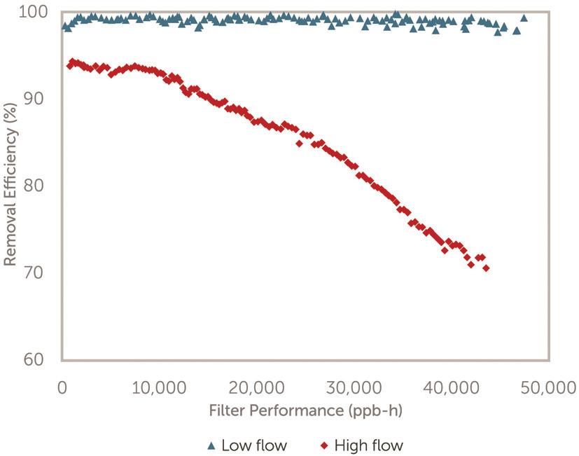
Typical AMC filter lifetimes are weeks to years, depending on application, filter design and desired removal efficiency. Two of the biggest impact parameters are AMC challenge concentrations and air flow rate. Higher concentrations use up available active adsorbent sites faster and higher flow rate reduces residence time on the adsorbent and with that, the overall removal efficiency. Figure 3 shows a typical performance curve for the removal of organic contaminants for two flow scenarios, low flow at 0.5 m/s face velocity and high flow at 2.5 m/s, using the same filter media.

How to Optimize Filter Lifetime?

The described “See it. Control it.” approach helps to define and understand individual applications and put analytical as well as filter performance results in proper context by knowing contaminants, their concentrations, the filter’s removal efficiency and lifetimes and considering process impact. This leads to minimizing cost of ownership and maximizing the performance with optimized filtration solutions.

In addition, monitoring contaminants over time not only defines the application’s contamination state better, but also reveals gradual environmental changes, which may require filter solutions to be adjusted to that change. Having a commercial analytical service to measure AMC or particles onsite is a critical necessity.

Measurement Accuracy Is Important

The cost of analytical evaluation typically scales with performance. In order to get enough insight into the contamination state of a space, measurements must be specific, selective and accurate. For gas-phase contaminants, corrosion strips, micro balances or other semi-quantitative means can be inexpensive, but are limited to qualitative answers at best, these systems do not provide accurate concentrations or identification of contaminants. Meaningful gas phase contamination should identify/speciate each contaminant, but also measure its concentration accurately with sufficient, statistically derived detection limits, ideally by an ISO 17025 accredited laboratory.

Semiconductor plants that operate at ppt concentration levels cannot be characterized with a local laboratory specializing in EPA type ambient air quantitation at the ppm level. Likewise, a product sensitive to submicron particle intrusion and protected by ULPA filters cannot be characterized with inexpensive particle counters that are made for PM 2.5 monitoring. A competent filter supplier should be able to help with the analytical evaluation as well as with putting data into the application’s context.

A Case Study

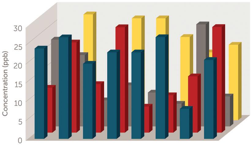
A semiconductor customer wanting to utilize AMC filters followed our “See it. Control it.” approach. As a first step, they characterized their cleanroom environment by measuring ammonia, a common contaminant that affects semiconductor circuitry, throughout the 40000 square foot large manufacturing space. Measurements were done in eight rows of four paths for a total of 32 measurement points. The idea was to find out how much the concentration of ammonia varied throughout the space, which, surprisingly, was between 4 and 20 ppb of ammonia (Figure 4) for an average of about 18 ppb. A single measurement might have not defined that average well enough.

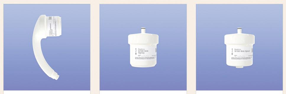
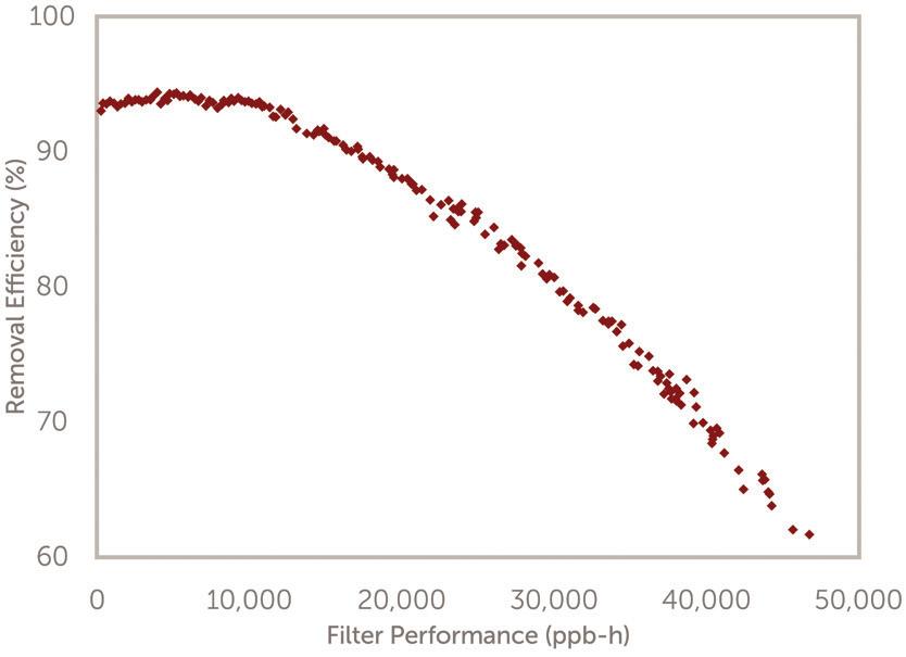
The second step then was to install AMC filters, which were maximizing the removal of ammonia, while also reducing organic contamination in the same space (a minor concern). Once that formulation was established, the customer used the performance curve of the filter as provided by the product sheet of the filter manufacturer, which shows removal efficiency of ammonia as a function of capacity (in ppb-h). This provided a reference point to calculate lifetime (Figure 5).

Once the filters were installed, ammonia concentrations were monitored over time. As Figure 6 shows, ammonia concentration successfully diminished as a function of the filter installation from an initial average of about 18 ppb to eventually level off at about 3.5 ppb.

Any concentration below 4 ppb was considered safe for the process at the time. The reason why concentration did not drop to zero is the fact that human bodies – the employees of that plant – naturally produce ammonia and emit it to the surrounding air. The leveled concentration was an equilibrium between ammonia production and removal.

When the average concentration trend exceeded the threshold of 4 ppb, defined by the process sensitivity, the contamination production exceeded its removal and the filter no longer protected the process. That is the time when the filter needed to be changed. Measurements need to be frequent enough to detect changes to avoid endangering the process, but also ensure to detect an upward trend, without relying on a single data point to make filter change decisions that could be very costly.

Iterating between that found lifetime (in this case: about one year) and the performance curve of the filter will yield the targeted removal efficiency of the installation. At an average AMC challenge of 7 ppb (from measurements taken upstream of the filter) and the determined one year lifetime (8700 hours) to filter exhaustion provides a value of about 60000 ppb-h capacity. Plugging that into Figure 4 would provide an end of life removal efficiency of 50%. That is what the customer established as the future lifetime definition. For subsequent installations, they only measured filter removal efficiency occasionally, rather than weekly. Once the filters approached 50% RE, new filters were ordered for replacement.

 Figure 6: Manufacturing plant environmental ammonia concentration observed over time. Once concentrations exceed the safe threshold (red data), filters need to be changed out.

By working together to get analytical expertise, evaluate filter performance and to put those data into context, the customer was able to extend filter lifetime until the threshold was determined below which the process was no longer affected, and the maximum tolerable lifetime of the filter and optimized cost of ownership. It is that iterative process that needs to be done initially, before a simple end of life definition can be adopted.

Limitations

Limitations to the shown paradigm apply if an industrial environment maintains many different spaces with very different contamination states and impacts. For example, a factory might have multiple assembly lines all using different chemicals, different amounts of employees with different air circulation flows an varying process sensitivities. Creating optimized solutions for each of these individual sub-space would lead to high inventory, longer lead times and higher cost for

References

1. Airborne Molecular Contamination (AMC) Solutions for Commercial Operations. Entegris white paper, September 2024. https://www.entegris.com/content/dam/shared-product-assets/ vaporsorb/brochure-airborne-molecular-contamination-solutions-for-the-microelectronics-industry-10092.pdf

2. Standard ISO 10121, Test method for assessing the performance of gas-phase air cleaning media and devices for general ventilation, International Standards Organization. https://www.iso.org/ search.html?PROD_isoorg_en%5Bquery%5D=ISO%2010121

3. Standard 52.2-2017, Method of Testing General Ventilation AirCleaning Devices for Removal Efficiency by Particle Size (ANSI Approved), ASHRAE. https://store.accuristech.com/ashrae/ standards/ashrae-52-2-2017?gateway_code=ashrae&product_ id=1942059 smaller purchase quantities and involved installation regimes. In these cases, purchasing a single filter for all environments will provide a better cost and lead time with simple inventory and installation routines, but will reduce applicability as the filters would be made to serve the least common denominator, instead of being optimizing for each sub-environment.

Another limitation is found in rapidly changing environments, where not only concentrations but also contaminant types change quickly over time. This would obsolete the best tailored solution quickly and demand a switch to a new solution in order to protect the process, increasing cost and not allowing to use filters up until their designated end of life. The same limitation applies here to any solution that tries to accommodate all contamination scenarios over time with less targeted contaminant removal.

Conclusions

We have shared and explained that the “See it. Control it.” approach to contamination control is well suited to optimize a filtration solution for longest filter lifetime, best performance and lowest cost of ownership. Accurate and competent analytical characterization as well as optimized filtration solutions are both required segments for this approach. We have shown how this applies to different filtration regimes and illustrated it with a real world case study. Some limitations apply to this scenario, but for most practical purposes, it is a valid and useful tool for contamination control management. www.entegris.com

Jürgen Lobert is a Director of AMC Technology at Entegris, Inc. with more than 20 years of experience in the measurement and filtration of gasphase (molecular) contamination. For another 20 years prior to that, he studied atmospheric chemistry and various sources and sinks for air pollutants and building advanced measurement technologies. Jürgen is the author of more than 60 publications on air chemistry and contamination control and he is a member of standards committees for SEMI and the IRDS.

4. Standard ISO 29463, High efficiency filters and filter media for removing particles from air, International Standards Organization. https://www.iso.org/search.html?PROD_isoorg_ en%5Bquery%5D=ISO%2029463

5. Standard ISO 5725, Accuracy (trueness and precision) of measurement methods and results, International Standards Organization. https://www.iso.org/standard/69418.html

6. Targeted Removal Assures Purity in Advanced Materials, Entegris, Inc., https://www.entegris.com/content/dam/web/ resources/pictograms/pictogram-targeted-removal-assurespurity-in-advanced-materials-12335.pdf