Mathematical Analysis of Car & Bridge Interaction Using Law of Physics for Vibration Formulation

Mr. Avinash Gavel1 , Dr. H. R. Suryawanshi2 , Mr. Sudheshwar Singh3

Abstract: Vibration is the natural & inherent property of resistance against disturbance in a Elasto-Plastic materials. The structure are often designed in the manner that they can sustain and maintain their superstructure under the influence of dead and live loads with the minimum disturbance of their inertia. The super-structures and tunnels are generally placed on the surface of load carrying columns in the form of simply supported beams. The integration method of which generates a continuous system which is the bridge super structure. So that Natural Frequency (time function Fn) and Response Function (space function) can be generated and programmed in MATLAB.

Keywords: Vibration, formulation, space function, continuous system

I. INTRODUCTION

The first mathematical expressions were developed in the late 1990’s carrying out many experiments by C. E. Inglis for Tracks considering simply supported segments of a continuous system and S. Timoshenko for bridge super structures. In both of the cases the bridge is the integrated system of simply supported segments containing a lumped vehicle mass. The experiments of 1950’s were also lab dependent until the 1970’s. At that time computer was available for designing and simulating the bridge parameters. Dynamic analysis was firstly carried out in 1953 by K. H. Kinnier. After the year 1980’s standard composite materials like Portland cement, ceramics and RCC were being used extensively in place of steel bridges which were providing flexibility with complexity in material property and geometry. The advancement of new mathematical expression using Laplace and Newmark beta function provides accurate results of damped frequency and damping co-efficient for either side of the vehicle at each point of the bridge using Delta function.

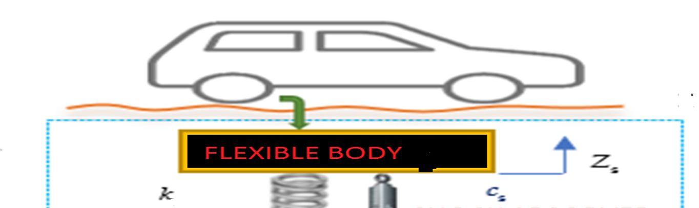
Transport vehicle and bridge both reflects complex models in the real environment. At the point of interaction the damping systems and wheels diminish the value of vibration of assembly up to a very high limit. The structure itself behaves like a damper. During the analysis of vibration the vehicle is considered as a concentrated mass.

Fig (a):- Load amplitude curve of cosine function in domain (-π, π)

Figure (a) shows the effects of bumps over the vehicle and its mathematical model. The value of damping always varies from zero to unity. A wave has thenature of diminishing its amplitude with respect to time. Thereduction of amplitude is inverselyproportional to thefrequencyof vibrationof the bridge as well as of the automobile also.

ISSN: 2321-9653; IC Value: 45.98; SJ Impact Factor: 7.538

Volume 11 Issue II Feb 2023- Available at www.ijraset.com

In Fig.2 represents the elastic behavior of an eccentric vehicle which has following parameters.

1) Pitching angle (ϴ).

2) Eccentricity of support from the center of mass (l1 and l2 respectively).

3) Deviation of mass -center (x).

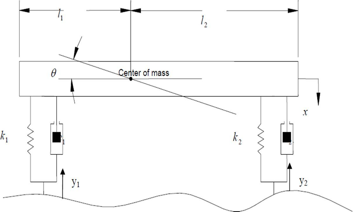
4) Lift of the tyre (y1 and y2) i.e. displacement of wheels in vertical direction.

5) Equivalent stiffness (k1 and k2) and equivalent damping (c1 and c2 ) respectively for the automobiles front and rear elements

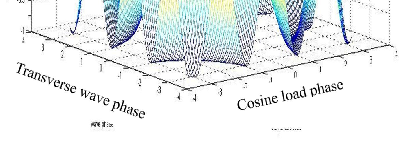
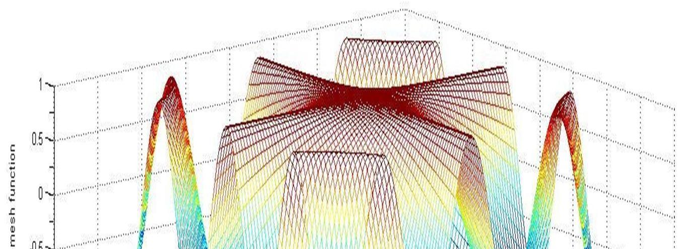
Figure 3.2 represents two perpendicular curvilinear co-ordinates representing highest amplitude of vibration at the center of bridge irrespective to the position of load for the first shape mode of vibration.

Explanation of parameters:- A complex vehicle structure is made up of robust assemblies and meeting parts having complex moving structures. The analysis commonly used for design considerations are:- a) Unidirectional axle 2D model b) Double axle 2D model with four degree of freedom. c) 3 Dimensional models with seven degree of freedom.

ISSN: 2321-9653; IC Value: 45.98; SJ Impact Factor: 7.538

Volume 11 Issue II Feb 2023- Available at www.ijraset.com

In this, 2D model of vehicle has been used having properties stiffness (k), damping(c) and mass (m) matrices with the interactional behavior of bridge material. Mainly the lower order natural frequency is introduced which is the basic mode of vibration. The bridge is assumed to be made up of the simply supported segments of homogenous material. Mode superposition method is used to reduce the degree of freedom. The dynamic analysis is done with superposition of load along with the Euler Bernoulli beam theory.

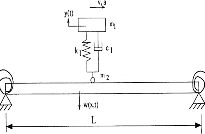
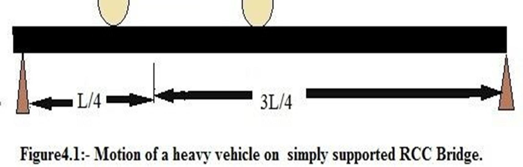
Here, w(x, t) is the uniform shape function of load density. L is the length of the structure. V is the velocity of the vehicle a is the position of rear wheels. Other terms have their usual meanings.

Figure (3) shows that the position of moving vehicle is the function of velocity and corresponding time. The vehicles as well as the bridge material also have damping properties. Unbalancing of vehicle and bridge are the result of relative motion between them because the point contact of bridge and vehicle changes with time to time. The hysteresis is the accumulation of load with time duration and speed of the vehicle increasing successively day by day.

II. PROCEDURE

Assumptions made at different stages of superposition: The bridge and the car both have to tackle the environmental parameters such as atmospheric pressure, speed of vehicle and density variation of air due to temperature and seasons etc. All the parameters could not be taken for the consideration. At the time of interaction of bridge and vehicle only material properties and surface properties are involved in the calculation of bridge vibration. At that instant positions of the rest parts of the vehicle other than the contact with bridge are considered as elements of lumped body. Assumptions made at different stage of superposition are as under: -

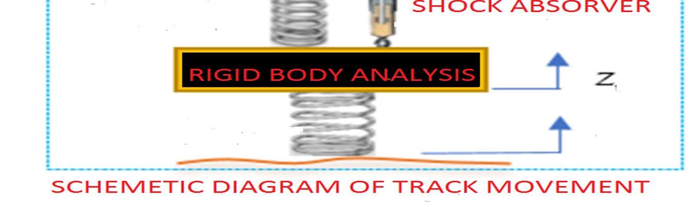
1) The automobile is assumed to be a rigid body during the calculation of vibration of bridge so that only bridge variables are considered as variables at that time.

2) The dead load is linear function of mass density for uniform propagation of amplitude function.

3) There is no transverse motion in bridge other than longitudinal direction.

4) The property of bridge (i.e. flexural rigidity EI and linear mass density ρ) remains constant during the motion of vehicle to evaluate length-time and length-density propagation.

5) The property of vibration after impulsive loading will be treated as a cosine function over the L length of the vehicle.

III. REASON OF CONSIDERING COSINE WAVE

The simplification of the bridge model, using the cosine function (including general bridge parameters) with the basic vibration parameters is the easiest way of calculating amplitude of bridge vibration. It is impossible to analyze all the bridge parameters with a single bridge model because of different types and manners of loadings. Cosine function due to its following properties:

1) Continuous function of space and time variables.

2) Differentiability of the function at each position of vehicle.

3) Single valued at each point of vibration.

4) The maximum and minimum magnitude is unity thorough out the length.

5) Whatever the domain (-∞, +∞), the range varies in the range [-1,1].

6) The fundamental range is from (-π, π) in which at the point of interaction, the cosine function has highest load as well as deflection value.

ISSN: 2321-9653; IC Value: 45.98; SJ Impact Factor: 7.538

Volume 11 Issue II Feb 2023- Available at www.ijraset.com

7) The maximum possible load value is considered at mid span interaction. All other points will be calculated in the fraction of maximum displacement due to cosine function.

IV. STEPS OF APPROACH

1) Selection of standard elastio-plastic bridge material (i.e. concrete).

2) Function of bridge vibration should be progressive within the length and unchanged to the surrounding. Wave equation is suitable under impulse load of vehicle with point contact of bridge and wheel for the bridge. Euler Bernoulli beam theory relates the material properties (EI and ρ) with the amplitude functions of front and rear wheels in the terms of time and position.

3) Utilization of impulse loading under finite length span of bridge provides shape function of amplitude and time function of frequency for different modes. Laplace transform of integral provides an exact solution of space- time functions in orthogonal (free) co-ordinates.

4) Location of the wheel is the time-velocity product, on the bridge. After crossing the bridge deflection of vehicle and bridge are independent to mutual interaction.

5) Effective deviation of wheel is the function of position on the bridge and eccentric load due to own weight within the bridge.

6) The shape function of wheels are valid from the entry of front wheel on the bridge i.e. (a/v), to the exit of rear wheel (l+a)/v from the bridge.

7) Analysis of variation of natural frequency with density of bridge material and length using MATLAB.

8) After the analysis of bridge, the eccentric load on the vehicle is also required to be quantified. This is carried out by calculating frequency of the standard vehicle using complex function and MATLAB. The input parameters are distance of wheel positions from center of gravity of vehicle, stiffness and damping co-efficient of front and rear wheels.

9) The damping ratio is calculated with the help of complex roots of natural frequency of four wheels.

10) These complex roots also provide the resultant of mode shape (plane) and its propagation from wave direction. Then transfer function is generated mathematically including all the parameters. Laplace function provides exact solution for load transfer ratio with Cremer rule.

V. TRANSVERSE STATIC VIBRATION ANALYSIS

1) There are two ways of analyzing vehicle vibration

2) Stationery bridge and moving vehicle for analyzing vehicle behavior.

3) Moving bridge carrying lumped vehicle mass.

The combination of these two ways of analysis will provide high degree of accuracy in analysis of each parameter of bridge design. For an example the static loading frequency is calculated by load per unit deflection. If a vehicle of 10 tons is moving on the concrete bridge. The static transverse deflection of bridge is 3/2 mm. then natural frequency can be calculated without considering the gravity load as following: