International Journal for Research in Applied Science & Engineering Technology (IJRASET)

ISSN: 2321-9653; IC Value: 45.98; SJ Impact Factor: 7.538

Volume 11 Issue I Jan 2023- Available at www.ijraset.com

Tablei

Different Boundaries

Boundary Conditions in ANSYS Fluent 2020 R1

Inlet Velocity Inlet

Ground Surface and Hill Wall [No Slip Wall]

Top and Side Walls of Domain Symmetrical [Free Slip Wall]

Tall Building Wall [No Slip Wall]

Outlet

Constant Pressure Outlet

III.NUMERICALSTUDY

The k - ɛ (Realizable) model is widely utilised in the field of Computational Fluid Dynamics (CFD). The gradient diffusion hypothesis may be used to establish a connection between Reynolds stresses, mean velocity gradients, and turbulent viscosity. The intensity of the turbulence was set at 10%. When a turbulent velocity and a turbulent length scale are multiplied together, the resulting turbulent viscosity is computed. The turbulence kinetic energy, denoted by the symbol “k”, is defined as the variance of the variations in velocity. It has the dimensions (L2T2); for example, m2/s2. The turbulent eddy dissipation “ɛ” is a kind of eddy dissipation. It has per unit time (L2T3) dimensions, which are equivalent to m2/s3. The k - ɛ model introduction of two new variables into the equation system. The following is the continuity equation:

Momentum and conservation:

Turbulent kinetic energy, k equation eddy dissipation rate “ɛ” equation.

Where µt is denotes as eddy viscosity, Gk is known as the creation of turbulence kinetic energy due to mean velocity gradients, and Gb is known as the generation of turbulence kinetic energy due to buoyancy, respectively. The contribution of variable dilatation in compressible turbulence to the total dissipation rate is represented by Ym µ is the component of the flow velocity that is parallel to the gravitational vector, and ν is the component of the flow velocity that is perpendicular to the gravitational vector. C3ɛ is also a constant, whose value is determined by µ and ν.

A. Solver Setting

All of the outcomes were steady-state in nature. Second-order differencing was used for the pressure, momentum, and turbulence equations, as well as the "coupled" pressure-velocity coupling approach, which is more durable for steady-state, single-phase flow problems. After many hundreds of trials, the residuals dropped below the commonly accepted 10-4 limit. During the simulation, the drag force and average pressure value impacting on the tall structure were measured, and the simulations were regarded to have converged only when they reached stable and constant values. Even though the simulations were steady-state, the "stable" values of the continuous monitoring data ranged by around 1%. In ANSYS Fluent 2020 R1, both buildings were considered as a bluff body (a body that is angular but not aerodynamic in form), and the flow pattern around the isolated square shape building and under the interference condition due to the hill were analysed under various conditions. Table – 5 of IS: 875 (Part 3), 2015 [2] contains the external pressure coefficient (Cpe). Following the fulfilment of certain requirements, the value of the external pressure coefficient is examined. It has been determined that the requirement 3/2 < h/w < 6, 1 < l/w ≤ 1/2 is fulfilled with Table: 4 of IS: 875 (Part 3), 2015 [2] in this research. Where "H" denotes the bluff body’s height above mean ground level, "w" denotes the width or smaller horizontal dimension of a bluff body, and "l" is denoting the length or larger horizontal dimension of a bluff body, as defined in IS: 875 (Part 3), 2015 [2] for the examination of the reliability of the software.

ISSN: 2321-9653; IC Value: 45.98; SJ Impact Factor: 7.538

Volume 11 Issue I Jan 2023- Available at www.ijraset.com

B. Examination of the reliability of ANSYS Fluent Software based on a comparative analysis of the findings of a square shape building model

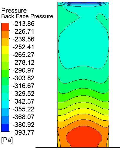
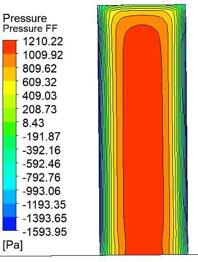
As illustrated in Fig. 5, the pressure distribution on different faces of a square-shaped building model with an aspect ratio “h/w” considered 3 for the reliability of software for wind incidence angles of 0° is presented on different faces of the square shape building model. Pressure on the windward face is positive, as expected, with the highest pressure in the center of the windward facing area. Moreover, since wind flow displays symmetry, pressure distribution is symmetrical around the vertical centerline. In addition, there is a thin line of significant negative pressure towards the windward face, which causes suction on the side faces. This is caused by the flow being separated from the edges of the windward face. Because of the symmetry of wind flow, the pressure distributions on the two side faces are identical. On the leeward face, suction is also present; however, this time, the pressure is equally distributed along the horizontal line. As shown in Table 3, the findings obtained for the square model are compared with those accessible in the IS: 875 (Part 3), 2015 [2], which are included in the IS: 875 (Part 3), 2015 [2] and value published by the researcher found by the wind tunnel experimental.

The wind pressure was evaluated with the wind incidence angle set to 0° on the windward and leeward faces of the tall building, the mean pressure was measured at the windward and leeward faces. In addition, maximum pressure values were determined for each face of the tall building, and the drag coefficient was computed at different positions along the tall building's length in respect to the hill. By using the Equation 7, we were able to convert these pressures into pressure coefficients, which is a dimensionless number that reflects how pressure is distributed on all side faces of a tall building and varies based on the tall building's location in reference to a 3-dimensional hill.

The investigation of the square shape building model included the analysis of a principal building in an isolated condition in ANSYS Fluent 2020 R1 in order to verify its acceptability and reliability in assessing pressure coefficient in accordance with the IS: 875 (Part 3), 2015 [2], and value published in research paper.

ISSN: 2321-9653; IC Value: 45.98; SJ Impact Factor: 7.538

Volume 11 Issue I Jan 2023- Available at www.ijraset.com

The findings show that the ANSYS Fluent 2020 R1 has a high degree of consistency, with the results being pretty close to the IS: 875 (Part 3), 2015 [2] prescribed values of pressure coefficients as well as result published by the researcher in research paper shown in Table 3. As a result, the data considered for the principal building in isolated condition can be used to evaluate the pressure coefficient under the interference condition of hill in a complex region for different spacing ratios between the hill and the square shape building using the ANSYS Fluent 2020 R1 software. This allows for the necessary investigation. TABLE

Iiiii

IV.RESULTANDDISCUSSIONS

A. Flow analysis for a hill with no tall buildings

At three different locations along on the symmetrical vertical plane, wind velocity profiles are shown in Figure 6. One is at a point on the windward side of a hill, the second is on the leeward side of the hill, and finally, the third is at the top of the hill. The k ɛ (Realizable) turbulence model is used in this study to calculate wind flow analysis. ANSYS turbulence model predicts velocities that are very close to the flow physics. hills without buildings have been used as a research study in this investigation. The velocity profile shown in Fig 6 shows the wind velocity profile at three locations and higher wind is near the top of the hill's top. The maximum speed of 55.47 m/s was attained towards the top of the hill. Once at the top, the 44 m/s speed progressively reduces in a vertical direction.

Fig. 6 Velocity Profile at three Different Locations

For the 85-meter-high hill in Fig 5, the pressure contour diagram is shown on a symmetrical vertical plane at y = 0, with the wind direction taken into account from left to right. The incoming velocity of 44 m/s is uniform and progressively rises from ground level because to the thin boundary layer near the ground. As the boundary layer reaches the top of the top of the hill in Fig.7, it grows rapidly as a result of the considerable negative pressure gradient. Wind flow acceleration is only influenced in small places at the top of the hill, where the boundary layer is getting thinner, since the boundary layer is becoming increasingly thin. Generally, the top of a hill is considered a high-speed zone. After the hill, the boundary layer thickens, creating a low-speed zone behind the leeward side. Flow doesn't seem to separate on the leeward side.