International Journal for Research in Applied Science & Engineering Technology (IJRASET)

ISSN: 2321-9653; IC Value: 45.98; SJ Impact Factor: 7.538

Volume 11 Issue III Mar 2023- Available at www.ijraset.com

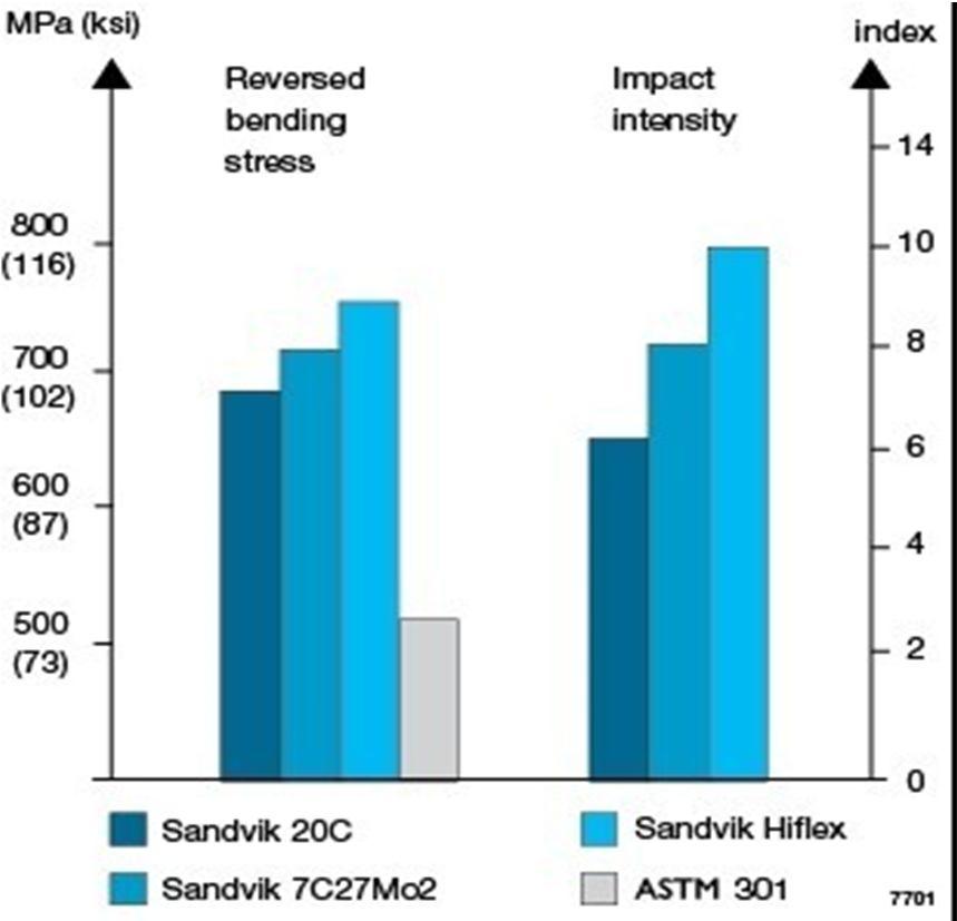
GRAPH 1. Comparison of fatigue properties for sandvik’s flapper valve steels and standard spring steel (ASTM301)

IV. PROJECT METHODOLY

A. Specimen Flapper Valve

2 test valve specimens were prepared for the experimental work. The material valve was standard spring steel ASTM301 and Sandvik spring steel 20C.

ISSN: 2321-9653; IC Value: 45.98; SJ Impact Factor: 7.538

Volume 11 Issue III Mar 2023- Available at www.ijraset.com

B. Design of Valve

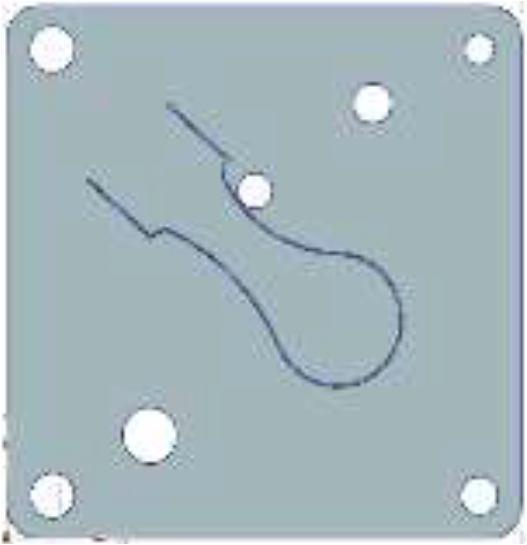
Desugn of Valve flap is done in siemens NX CAD software having same dimensions as that of available in market.

3 Flap Valve In Cad Model

V. A GENERAL OPERATION FOR ANALYSIS FACILITY

Certain steps in formulating a finite element analysis of a physical problem are common to all such analysis, whether structural, heat transfer, fluid flow, or some other problem. These steps are embodied in commercial finite element software packages (some are mentioned in the following paragraphs) and are implicitly incorporated in this text, although we do not necessarily refer to the steps explicitly. The steps are described as follows.

A. Preprocessing

The preprocessing step is, quite generally, described as defining the model and includes

1) Define the geometric domain of the problem.

2) Define the element type(s) to be used.

3) Define the material properties of the elements.

4) Define the geometric properties of the elements (length, area, and the like).

5) Define the element connectivity (mesh the model).

6) Define the physical constraints (boundary conditions).

7) Define the loadings.

The preprocessing (model definition) step is critical. In no case is there a better example of the computer-related axiom “garbage in, garbage out.”

A perfectly computed finite element solution is of absolutely no value if it corresponds to the wrong problem.

B. Solution

During the solution phase, finite element software assembles the governing algebraic equations in matrix form and computes the unknown values of the primary field variable(s). The computed values are then used by back substitution to compute additional, derived variables, such as reaction forces, element stresses, and heat flow. As it is not uncommon for a finite element model to be represented by tens of thousands of equations, special solution techniques are used to reduce data storage requirements and computation time. For static, linear problems, a wave front solver, based on Gauss elimination, is commonly used. While a complete discussion of the various algorithms is beyond the scope of this text, the interested reader will find a thorough discussion in the Bathe book.

C. Post Processing

Analysis and evaluation of the solution results is referred to as post processing. Postprocessor software contains sophisticated routines used for sorting, printing, and plotting selected results from a finite element solution. Examples of operations that can be accomplished include:

1) Sort element stresses in order of magnitude.

2) Check equilibrium.

3) Calculate factors of safety.

4) Plot deformed structural shape.