International Journal for Research in Applied Science & Engineering Technology (IJRASET)

ISSN: 2321-9653; IC Value: 45.98; SJ Impact Factor: 7.538

Volume 11 Issue III Mar 2023- Available at www.ijraset.com

4) Alanine Aminotransferase.

5) Aspartate Aminotransferase.

6) Total Proteins.

7) Albumin.

8) Albumin-to-Globulin Ratio.

9) The data were divided into two sets by a selector field (labelled by the experts).

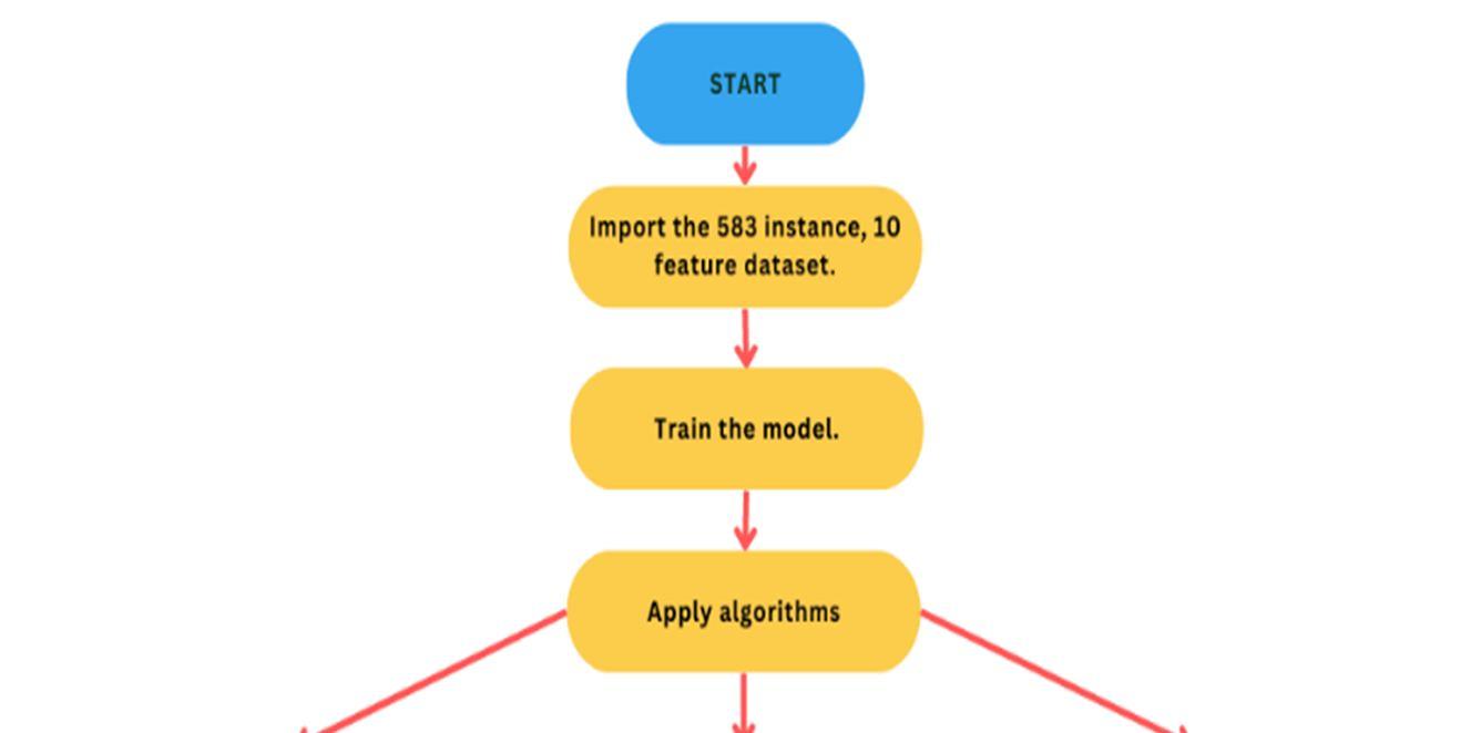
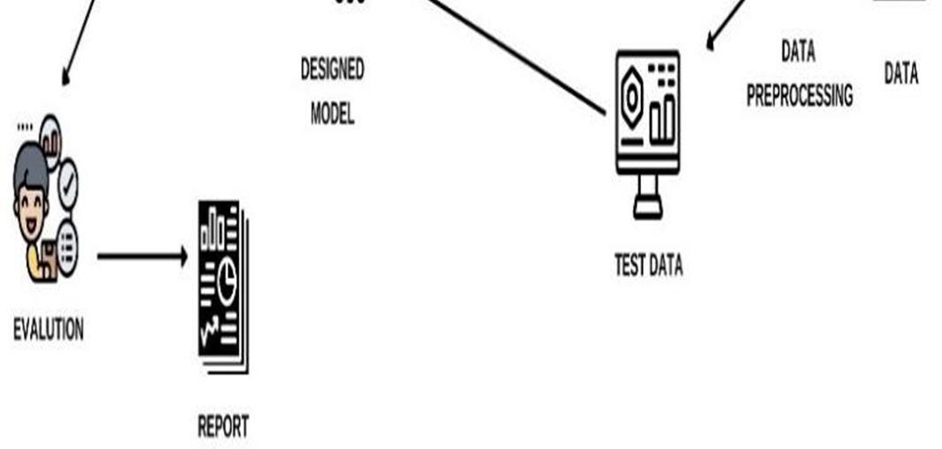
B. Data Preprocessing

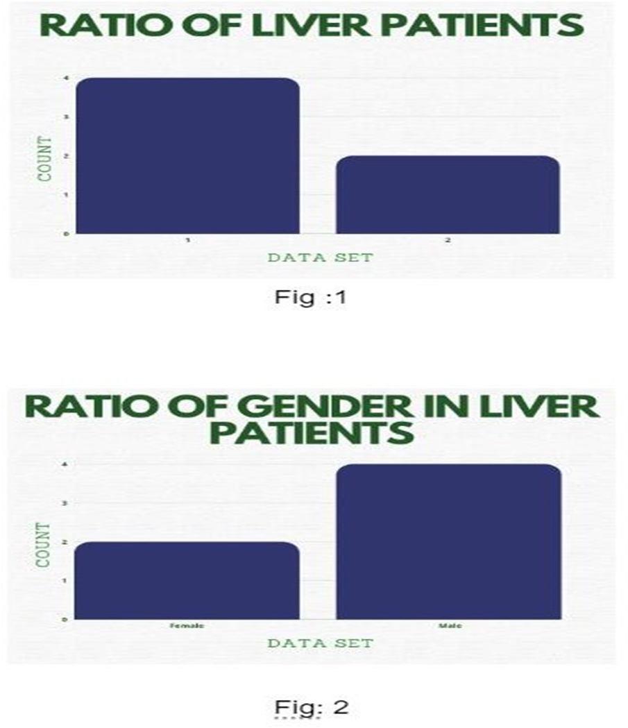
In this study, we examined the data of 583 liver patients, 416 of whom were liver patients and 167 of whom were not. Figure 1 depicts the ratio of total liver patients. Furthermore, 441 male samples and 112 female samples were taken for analysis from the liver patient's dataset (Fig. 2)

ISSN: 2321-9653; IC Value: 45.98; SJ Impact Factor: 7.538

Volume 11 Issue III Mar 2023- Available at www.ijraset.com

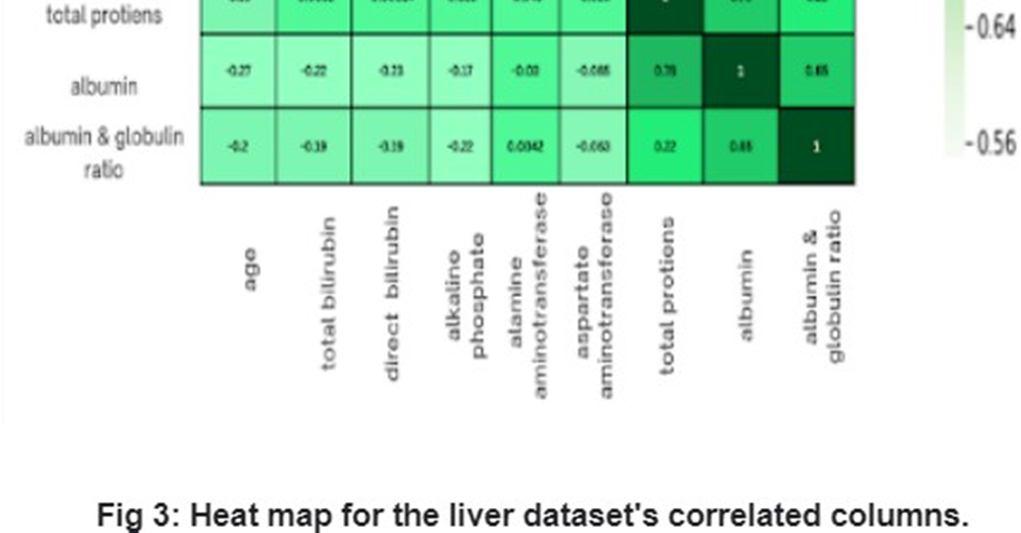
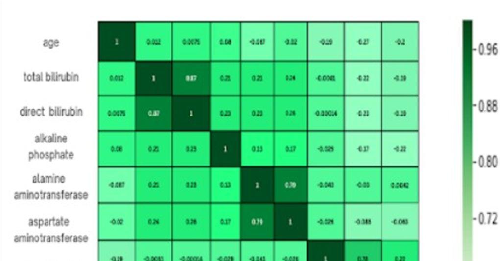
There are some associated characteristics in the heatmap in Fig. 3. These columns have a low correlation in some cases. In order to improve our ability to predict liver illness, we therefore removed some of the features.

C. Functional Requirements

The functional Requirements for the project are

1) Python 3.7 or later PIP for Windows.

2) Streamlit

3) Jupyter Notebook.

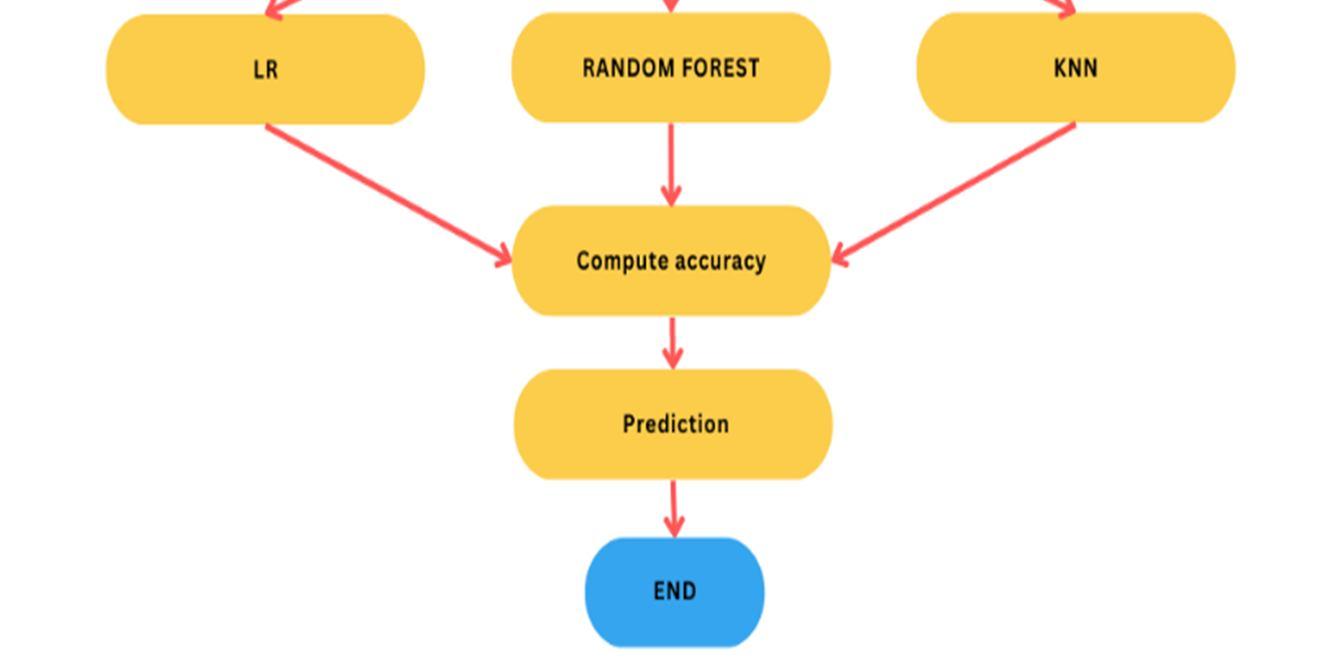
D. Representation of Classical Algorithms

1) Logistic Regression: By examining the correlation between one or more already present independent variables, a logistic regression model forecasts a dependant data variable. A logistic regression could be used, for instance, to forecast whether a candidate for office will win or lose, or if a high school student will be accepted into a particular institution or not. These simple choices between two options allow for binary outcomes. Many criteria for input can be taken into account using a logistic regression model. The logistic function can take into account the student's grade point average, SAT score, and number of extracurricular activities in the case of college acceptance. It then rates new cases according to their likelihood of falling into one of two outcome categories based on historical information about past outcomes involving the same input criteria. The technique of logistic regression has grown in significance in the field of machine learning. It enables machine learning algorithms to categorise incoming input based on previous data. The algorithms improve at predicting classes within data sets as more pertinent data is included. The technique of logistic regression has grown in significance in the field of machine learning. It enables machine learning algorithms to categorise incoming input based on previous data. The algorithms improve at predicting classes within data sets as more pertinent data is included. Logistic Regression model is implemented for the prediction of liver disease. The dependent variable ‘is_patient’ as ‘1’for yes and ‘0’ for no respectively are divided based on gender and plotted against the count of the patients. Logistic Regression can be used to classify the observations using different types of data and can easily determine the most effective variables used for the classification. The below image is showing the logistic function. Because it can classify new data using both continuous and discrete datasets, logistic regression is a key machine learning approach.

2) KNN: One of the simplest machine learning algorithms based on the supervised learning method is K-Nearest Neighbour. The K- NN algorithm places the new instance in the category that is most similar to the available categories based on the assumption that the new case and the available cases are comparable.

ISSN: 2321-9653; IC Value: 45.98; SJ Impact Factor: 7.538

Volume 11 Issue III Mar 2023- Available at www.ijraset.com

When a new data point is added, the K-NN algorithm classifies it based on how similar the existing data is to it and stores it all. This means that utilising the K-NN method, fresh data can be quickly and accurately categorised into a suitable category. Although the K-NN technique can be applied to classification and regression problems, it is most frequently utilised for classification issues. Since K-NN is a non-parametric technique, it makes no assumptions about the underlying data. It is also known as a lazy learner algorithm since it saves the training dataset rather than learning from it immediately. Instead, it uses the dataset to perform an action when classifying data. The KNN method simply saves the information during the training phase, and when it receives new data, it categorises it into a category that is quite similar to the new data.

3) Random forest: Random forests, also known as random decision forests, are an ensemble learning technique for classification, regression, and other assignments that generates the class that is the mean forecast (regression) or method of the classes (classification) of the individual decision trees. When a new set of samples is input into a random forest, each decision tree in the forest makes a prediction on this set of samples separately and integrates the prediction results of each tree to get a final result. This is done after the random forest has established a large number of decision trees in accordance with a specific random rule. This technique works by developing a large number of decision trees during training time. For decision trees' tendency to overfit their training set, random decision forests are the best option. There is an immediate relationship between the united trees and the result that the forest of trees can produce. To obtain forecasts that are more accurate and effective, random forest adds an additional layer of irregularity to the stowing. Based on the distinctive qualities and classification outcomes of a given dataset, Random Forest is a great supervised learning method that can train a model to predict which classification results in a particular sample type belong to. The decision tree-based Random Forest uses the "bagging" (bootstrap aggregating method) to generate various training sample sets. The best attribute from a group of attributes chosen at random is chosen by the random subspace division approach to divide internal nodes. The voting method is utilised to categorise the input samples, and the many decision trees created are used as weak classifiers. Multiple weak classifiers combine to construct a robust classifier. Each decision tree in the forest makes a prediction on this fresh set of samples independently after a random forest has built up a sizable number of decision trees in accordance with a certain random rule. The final result is obtained by integrating the prediction results of all the trees.

ISSN: 2321-9653; IC Value: 45.98; SJ Impact Factor: 7.538

Volume 11 Issue III Mar 2023- Available at www.ijraset.com

A. Classification of Evaluation Techniques

IV. RESULT

In our work, we employed certain genuine estimations to assess the test execution of various categorization algorithms. The various evaluation methodologies, such as accuracy, sensitivity, specificity, precision, and the f1 measure, were used to examine theperformance of the classification systems. As a result, the confusion matrix determines the exhibition assessment variables. In this case, true positive (TP): The prediction properly identifies a patient as having liver illness. False Positive (FP): The forecast wrongly identifies a patient as having liver disease. True Negative (TN): The conclusion of the prediction correctly rejects the patient's allegation of liver illness. False Negative (FN): The prediction result mistakenly eliminates the possibility that a patient has liver disease. The precision of the prediction model offers the difference between sound and patient capacity ratio. To establish classification precision, one must first determine the true positive, true negative, false positive, and false negative.

Accuracy = (TP+TN)/(TP+FP+FN+TN)

This effectability test successfully distinguishes patients with liver illness. It mostly demonstrates the test’s positive results.It is also known as recall and positive rate.

Sensitivity = (TP)/(TP+FN)

The negative repercussions of the condition are underlined in detail. It indicates the amount of the patients' missing sickness. It is also known as the "real negative rate" (TNR).

Sensitivity = (TN)/(FP+TN)

Positive predictive value is another name for precision. It displays the percentage of favourable outcomes that classifier algorithms accurately anticipated

Precision = (TP)/(TP+FP)

F1 combines accuracy and recall to determine the model's precision. It provides the model's FP and FN proportions. F1=(2*(R*P))/(R+P)

B. Analysis of the result

In this experiment, we examined three machine learning classifiers for the categorization of liver disease dataset using various techniques. After employing oversampling methods, KNN’s accuracy value was 70.28%. RF received 74.28%. The highest result was 76 57% for LR. The LR classification algorithm outperforms the other classifiers for predicting liver disease based on these measurement criteria.