Monojit Rudra, P Soni Reddy, Rajatsubhra Chakraborty, Partha Pratim Sarkar

International Journal of Advances in Applied Sciences (IJAAS)

Vol. 9, No. 4, December 2020, pp. 276~283 ISSN: 2252-8814, DOI: 10.11591/ijaas.v9.i4.pp276-283  276

Design of frequency selective surface comprising of dipoles using artificial neural network

Monojit Rudra1 , P Soni Reddy2 , Rajatsubhra Chakraborty3 , Partha Pratim Sarkar4 1,2,4Department of Engineering & Technological Studies, University of Kalyani, India 3Department of Computer Science and Engineering, Future Institute of Engineering and Management, India

Article Info

Article history:

Received Apr 16, 2020 Revised Jun 14, 2020 Accepted Jun 18 2020

Keywords:

ANN FSS MLP

ABSTRACT

This paper depicts the design of Frequency Selective Surface (FSS) comprising of dipoles using Artificial Neural Network (ANN). It has been observed that with the change of the dimensions and periodicity of FSS, the resonating frequency of the FSS changes. This change in resonating frequency has been studied and investigated using simulation software. The simulated data were used to train the proposed ANN models. The trained ANN models are found to predict the FSS characteristics precisely with negligible error. Compared to traditional EM simulation softwares (like ANSOFT Designer), the proposed technique using ANN models is found to significantly reduce the FSS design complexity and computational time. The FSS simulations were made using ANSOFT Designer v2 software and the neural network was designed using MATLAB software.

This is an open access article under the CC BY-SA license.

Corresponding Author:

Partha Pratim Sarkar, Department of Engineering & Technological studies, University of Kalyani, Nadia, West Bengal, 741235, India. Email: parthabe91@yahoo.co.in

1. INTRODUCTION

In microwave engineering, Frequency Selective Surfaces (FSSs) are planar periodic arrays of metal patches on a substrate or slots on a conducting sheet that function as a filter for free space radiation [1]. Many authors have made analysis on FSS through EM numerical methods, such as the Method of Moment [2]. But these numerical methods require high computational cost. So to avoid this, Artificial Neural Network (ANN) which are previously trained with results obtained by Method of Moment can be used for analysis of FSS [3-4]. Also, other algorithms like Genetic Algorithm (GA) and Particle Swarm Optimization (PSO) can be blended with ANN for faster and accurate training of the ANN [5–16]. In this paper, patch type FSS consisting of dipoles (as shown in Figure 1) is used whose dimensions (i.e. patch length ‘L’, patch width ‘W’, x-periodicity ‘Tx’ and y-periodicity ‘Ty’) are varied and the corresponding resonating frequencies are noted. Then using these simulated results, some neural network models are designed and trained, which can be used for faster analysis and design of FSS comprising of dipoles.

Int J Adv Appl Sci ISSN: 2252-8814

Figure 1. FSS comprising of dipoles: (a) geometry of unit cell, (b) geometry of array

2. BACKPROPAGATION TRAINING ALGORITHM

The Backpropagation is an algorithm for supervised training of ANN in which the error is propagated backward for update of weights of different layers of the neural network. A Multi-Layer Perceptron (MLP) is shown in Figure 2, having one input layer, one hidden layer and one output layer.

Figure 2. Example of an ANN model

The steps for Backpropagation Algorithm are as follows: 1. Weights and learning rate (α) are initialized Hidden Layer Weights: w1, w2, w3, w4 Output Layer Weights: w5, w6, w7, w8 Bias Weights: a1, a2, b1, b2 Learning Rate (α): 0.0001 2. Steps 3 to 10 are performed when stopping condition is false. 3. Steps 4 to 9 are performed for each training pair. 4. Each input unit receives input signal (ii) and sends it to the hidden unit. 5. Each hidden unit sums its weighted input signals to calculate the net input (net hi). net h1 = w1 i1 + w3 i2 + a1 net h2 = w2 i1 + w4 i2 + b1 Then an Activation function is applied to the net input to calculate the output of the hidden unit (hi). The output of the hidden layer is then sent to the output layer units. hi = f(net hi) Here Bipolar Sigmoid Activation Function is used: f(x) = 1 / (1 + e-x) 6. Similarly, for each output unit the net input (net oi) is calculated and the activation function is applied to compute the output signals (oi).

7. Each output unit receives a target pattern (ti) corresponding to the input training pattern (ii) and computes the error correction term(��i): ��1 = (t1 - o1) f '(net o1) ��2 = (t2 - o2) f '(net o2) Where, f '(x) is the derivative of f(x) These error correction terms are used to calculate the change in weights (Δwi) and change in bias weights (Δai and Δbi). Δw5 = α��1h1 Δa2 = α��1 SimilarlyΔw6, Δw7, Δw8 and Δb2 are calculated 8. Similarly each hidden unit calculates its error correction term(��i j): ��56 = ��1 w5 f '(net h1) + ��2 w6 f '(net h1) ��78 = ��1 w7 f '(net h2) + ��2 w8 f '(net h2) These error correction terms are used to calculate the change in weights and bias weights. Δw1 = α��56 i1 Δa1 = α��56 SimilarlyΔw2, Δw3, Δw4 and Δb1 are calculated 9. Each output unit and each hidden unit updates its bias weights and weights. wi(new)=wi(old) +Δwi ai (new)=ai (old) +Δai bi (new)=bi (old) +Δbi 10. The stopping condition is checked. The stopping condition may be certain number of epochs reached or when there is previously settled minimum error between actual output and target output.

3. RESEARCH METHOD

Here 5 MLPs are used. Each of them have 4 inputs and 1 output as shown in Figure 3, but the inputs and outputs are different as shown in Table 1.

Figure 3. Common ANN model for all 5 networks

Table 1. Inputs and outputs of the 5 MLPs

Neural Networks Inputs Output

Network 1 In Network 1, the 4 inputs are the length, width, xperiodicity and y-periodicity of the proposed FSS Network 2 In Network 2, the 4 inputs are the length, width, xperiodicity and resonant frequency of the proposed FSS Network 3 In Network 3, the 4 inputs are the length, width, resonant frequency and y-periodicity of the proposed FSS Network 4 In Network 4, the 4 inputs are the length, resonant frequency, x-periodicity and y-periodicity of the proposed FSS Network 5 In Network 5, the 4 inputs are the resonant frequency, width, x-periodicity and y-periodicity of the proposed FSS

In Network 1. The output is the resonant frequency of the proposed FSS In Network 2. The output is the y-periodicity of the proposed FSS In Network 3. The output is the x-periodicity of the proposed FSS In Network 4. The output is the width of the proposed FSS

In Network 5. The output is the length of the proposed FSS

Int J Adv Appl Sci ISSN: 2252-8814  279

4. RESULTS AND ANALYSIS

Initially, the proposed ANN models are trained using the simulation results obtained from ANSOFT Designer v2 software. The training data set is provided in Table 2.

Table 2. Training data set for ANN models

Patch Length Patch Width x-periodicity y-periodicity Step Size Data Set1 15 mm 1.5 mm 16.5 mm 2.4 mm–15 mm 0.9 mm Data Set2 15 mm 1.5 mm 18 mm 2.4 mm–15 mm 0.9 mm Data Set 3 15 mm 1.5 mm 19.5 mm 1.5 mm–15 mm 0.9 mm Data Set4 15 mm 1.5 mm 21 mm 2.4 mm–15 mm 0.9 mm Data Set5 15 mm 1.5 mm 22.5 mm 1.95 mm–15 mm 0.45 mm Data Set6 15 mm 1.5 mm 15.5 mm–22.5 mm 4.2 mm 0.5 mm Data Set7 15 mm 1.5 mm 15.5 mm–22.5 mm 6.9 mm 0.5 mm Data Set8 15 mm 1.5 mm 15.5 mm–22.5 mm 9.6 mm 0.5 mm Data Set9 15 mm 1.5 mm 15.5 mm–22.5 mm 12.3 mm 0.5 mm Data Set10 15 mm 1.5 mm 15.5 mm–22.5 mm 15 mm 0.5 mm Data Set11 9 mm 1.2 mm–2 mm 22.5 mm 15 mm 0.3 mm Data Set12 12 mm 0.5 mm–2 mm 22.5 mm 15 mm 0.1 mm Data Set13 15 mm 0.1 mm–1.5 mm 22.5 mm 15 mm 0.1 mm Data Set14 6 mm–20 mm 0.7 mm 22.5 mm 15 mm 1 mm Data Set15 6 mm–20 mm 0.9 mm 22.5 mm 15 mm 1 mm Data Set16 6 mm–20 mm 1.1 mm 22.5 mm 15 mm 1 mm Data Set17 7 mm–20 mm 1.3 mm 22.5 mm 15 mm 1 mm Data Set18 7 mm–20 mm 1.5 mm 22.5 mm 15 mm 1 mm

Next, the performance of the proposed ANN models in accurately predicting the FSS characteristics is validated using a test data. Here, an FSS comprising of dipoles having dimensionsL = 15 mm, W = 1.5 mm, Tx = 22 mm, Ty = 8 mm (as shown in Figure. 1) is used as a test data for the proposed ANN model validation. The dimensions considered here for testing the ANN models is not included in the data set used for training the MLPs. The FSS is simulated using ANSOFT Designer v2 software and its resonant frequency obtained is 8.15 GHz. Next, this data is used for checking the error of all the 5 MLPs, as shown in Table 3. Finally, the 1st MLP (having L, W, Tx and Ty as inputs and resonating frequency (RF) as output) is used to perform parametric study as given in Section 4.2.

4.1. Single value check (interpolation) of the proposed ANN

The validation result of the 5 MLPs using the single test data is given in Table 3. MLP1 is found to predict the resonating frequency (RF) of the FSS for the given set of FSS design parameters with 0.076% error. MLP 2–5 predicts the FSS design parameter (y-periodicity, x-periodicity, Patch Width, and Patch Length, respectively) with 0.94%, 1.724%, 0.0298%, and 0.056% error, respectively for the given input set as shown in Table 3.

Table3. Result for single value check (interpolation)

ANN Network Input 1 Input 2 Input 3 Input 4 Simulated Output

MLP 1 Patch Length 15 mm Patch Width 1.5 mm x-periodicity 22 mm y-periodicity 8 mm

RF 8.15 GHz

MLP 2 Patch Length 15 mm Patch Width 1.5 mm x-periodicity 22 mm

RF 8.15 GHz y-periodicity 8 mm

MLP 3 Patch Length 15 mm MLP 4 Patch Length 15 mm Patch Width 1.5 mm x-periodicity 22 mm y-periodicity 8 mm y-periodicity 8 mm

RF 8.15 GHz RF 8.15 GHz x-periodicity 22 mm Patch Width 1.5 mm

MLP 5 Patch Width 1.5 mm x-periodicity 22 mm y-periodicity 8 mm

RF 8.15 GHz Patch Length 15 mm ANN Output % Error

RF 8.1562 GHz y-periodicity 8.0754 mm x-periodicity 21.6207 mm Patch Width 1.4996 mm Patch Length 15.0084 mm 0.076 %

0.94 %

1.724 %

0.0298 %

0.056 %

An FSS is fabricated using parameters corresponding to MLP1 given in Table 3. The fabricated prototype is shown in Figure 4(a). The transmission characteristic of the fabricated FSS is measured using R&S VNA (ZNB20) and Tx/Rx horn antennas. The simulated and measured transmission (S21) characteristic of the fabricated FSS is given in Figure 4(b). It is found that the resonant frequency of the proposed FSS is nearly same in both simulation and measurement.

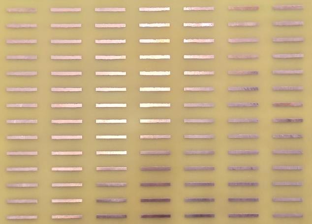
(a) (b)

Figure 4. (a) Fabricated prototype of the proposed FSS, (b) Simulated and measured transmission characteristics of the proposed FSS

4.2. Parametric study

In this section, extensive study has been conducted to test the performance of MLP 1. MLP 1 can only provide the resonating frequency (RF) as the output for the change in FSS design parameters- Patch Length, Patch Width, x-periodicity and y-periodicity. The values of FSS design parameters for this parametric study are tabulated in Table 4. Here, comparison is done between the simulated result obtained from Ansoft Designer and ANN.

Table 4. Data for parametric study

Constant Parameters Variable Parameters

Parametric Study 1 Patch Width = 1.5 mm, x-periodicity = 22.5 mm, yperiodicity = 15 mm Parametric Study 2 Patch Length = 15 mm, x-periodicity = 22.5 mm, yperiodicity = 15 mm Parametric Study 3 Patch Length = 15 mm, Patch Width = 1.5 mm, yperiodicity = 12.3 mm Parametric Study 4 Patch Length = 15 mm, Patch Width = 1.5 mm, xperiodicity = 22.5 mm

Patch Length = 7 mm to 20 mm with step 1 mm Patch Width = 0.1 mm to 1.5 mm with step 0.1 mm x-periodicity = 15.5 mm to 22.5 mm with step 0.5 mm y-periodicity = 1.95 mm to 15 mm with step 0.45 mm

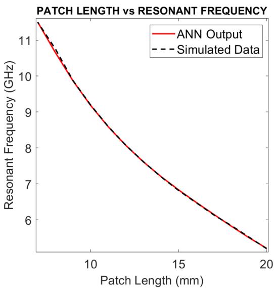
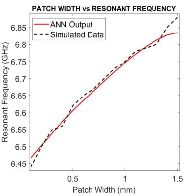
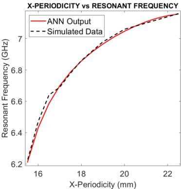
Figure 5 shows the results of Parametric Study 1 where Patch Width, x-periodicity, y-periodicityare kept constant and Patch Length is varied. Figure 6 shows the results of Parametric Study 2 where Patch Length, x-periodicity, y-periodicity are kept constant and Patch Width is varied. In Figure 7 the results of Parametric Study 3 is given where Patch Length, Patch Width, y-periodicity are kept constant and xperiodicity is varied. Figure 8 shows the results of Parametric Study 4 where Patch Length, Patch Width, xperiodicity are kept constant and y-periodicity is varied.

Int J Adv Appl Sci ISSN: 2252-8814  281

Figure 5. Results of parametric study 1: Variation of patch length from 7 mm to 20 mm with step 1 mm

Figure 6. Results of parametric study 2: Variation of patch width from 0.1 mm to 1.5 mm with step 0.1 mm

Figure 7. Results of parametric study 3: variation of X-periodicity from 15.5 mm to 22.5 mm with step 0.5 mm

Figure 8. Results of parametric study 4: variation of Y-periodicity from 1.95 mm to 15 mm with step 0.45 mm

4.3. Performance comparison of the proposed technique using ANN with traditional EM simulation software (like Ansoft Designer)

In traditional EM simulation software, analysis on FSS is done using EM numerical methods, such as the Method of Moment (MOM). These numerical methods require high computational cost, so even with a system with high configuration, the simulation time remains very long. But if instead ANN is used, then it doesn’t require any complex numerical methods, so naturally the computation time is reduced as compared to traditional EM simulation software. Here, firstly an FSS with patch-length = 15 mm, patch-width = 1.5 mm,

Design of frequency selective surface comprising of dipoles using artificial neural network (Monojit Rudra)

x-periodicity = 22.5 mm and y-periodicity = 15 mm is taken. |S21| vs. Frequency plot is done from 2 GHz to 12 GHz with low step count and for this the time elapsed is 6 minutes. From this plot the approximate resonant frequency is located somewhere between 6 GHz and 7.5 GHz. Then again plot is done from 6 GHz to 7.5 GHz with high step count which took 2 minutes time and the resonant frequency obtained is 6.83 GHz. So, the total simulation time required is 8 minutes. Then an FSS with patch-length = 8 mm, patch-width = 0.9 mm, x-periodicity = 22.5 mm and yperiodicity = 15 mm is taken. |S21| vs. Frequency plot is done from 2 GHz to 12 GHz with low step count and for this the time elapsed is 4 minutes. From this plot the approximate resonant frequency is located somewhere between 10 GHz and 11.5 GHz. Then again plot is done from 10 GHz to 11.5 GHz with high step count which took 2 minutes time and the resonant frequency obtained is 10.76 GHz. So, total simulation time required is 6 minutes. But in case of ANN, generation of |S21| vs. Frequency plot is not required, as it directly gives resonant frequency as output. In first case the resonant frequency obtained is 6.8348 GHz, and in the second case the resonant frequency obtained is 10.7404 GHz. Here in both the cases the ANN gave resonant frequency output in less than 1 sec time (i.e. in the first case 0.36036 sec and in the second case 0.27701 sec). The percentage reduction in computational time is 99.9249 % in the first case and 99.9230 % in the second case, as shown in Table 5.

Table 5. Performance comparison of the proposed technique using ANN with traditional EM simulation software

Parameters Simulation Time ANN Output Time % Reduction

patch-length = 15 mm patch-width = 1.5 mm x-periodicity = 22.5 mm y-periodicity = 15 mm patch-length = 8 mm patch-width = 0.9 mm x-periodicity = 22.5 mm y-periodicity = 15 mm 8 minutes 0.36036 sec 99.9249 %

6 minutes 0.27701 sec 99.9230 %

5. CONCLUSION

In this paper, an Artificial Neural Network model is trained using data obtained from ANSOFT Designer v2 software which uses Method of Moment for analysis of FSS. Hence, the ANN is properly trained and gives negligible error. Using this ANN, the results are obtained very quickly which saves time and also reduces the computational cost and complexity.

REFERENCES

[1] Ben A. Munk, “Frequency Selective Surfaces – Theory and Design,” Wiley, no. 1, pp. 1-5, 2000. [2] Jianxun Su and Xiaowen Xu, “MOM analysis of the planar and curved FSS based on dipole elements,

” International Conference on Microwave Technology and Computational Electromagnetics (ICMTCE 2009), Beijing, China, pp. 127-130, 2009. [3] P.L. da Silva and A.G. D’Assuncao, “Neuromodelling of Frequency Selective Surfaces and E-Shaped Microstrip

Antennas, ” The 2006 IEEE International Joint Conference on Neural Network Proceedings, Vancouver, BC, Canada, pp. 2374-2377, 2006. [4] P.H.F. Silva and A.L.P.S. Campos, “Fast and accurate modelling of frequency selective surfaces using a new modular neural network configuration of multilayer perceptrons, ” IET Microwaves, Antennas & Propagation, vol. 2, no. 5, pp. 503-511, 2008. [5] P.H. da F. Silva, P. Lacouth, G. Fontgalland, A.L.P.S. Campos and A.G. D’Assuncao, “Design of frequency selective surfaces using a novel MoM-ANN-GA technique, ” 2007 SBMO/IEEE MTT-S International Microwave and Optoelectronics Conference, Brazil, pp. 275-279, 2007. [6] R.M.S. Cruz, P.H. da F. Silva and A.G. D’Assuncao, “Synthesis of crossed dipole frequency selective surfaces using genetic algorithms and artificial neural networks, ” 2009 International Joint Conference on Neural Networks, Atlanta, GA, USA, pp. 627-633, 2009. [7] P.H. da F. Silva, R.M.S. Cruz and A.G. D’Assunção, “Blending PSO and ANN for Optimal Design of FSS Filters

With Koch Island Patch Elements, ” IEEE Transactions on Magnetics, vol. 46, no. 8, pp. 3010-3013, 2010. [8] Anuradha, A. Patnaik, S.N Sinha and J.R. Mosig, “Design of customized fractal FSS, ” Proceedings of the 2012 IEEE International Symposium on Antennas and Propagation, Chicago, IL, USA, 2012. [9] M.R. da Silva, C. de L. Nóbrega, P.H. da F. Silva and A.G. D’Assunção, “Optimal design of frequency selective surfaces with fractal motifs, ” IET Microwaves, Antennas & Propagation, vol. 8, no 9, pp. 627-631, 2014.

Int J Adv Appl Sci ISSN: 2252-8814  283

[10] W. C. Araujo, A. G. D’Assunção Junior, E. E. C. Oliveira and A. G. D’Assunção, “FSS designs using a populationbased hybrid algorithm inspired on the echolocation of bats, ” 2015 9th European Conference on Antennas and Propagation (EuCAP), Lisbon, Portugal, 2015. [11] M. C. Alcântara Neto, F. J. B. Barros, J. P. L. Araújo, H. S. Gomes, G. P. S. Cavalcante and A. G. D’Assunção,

“A metaheuristic hybrid optimization technique for designing broadband FSS, ” 2015 SBMO/IEEE MTT-S International Microwave and Optoelectronics Conference (IMOC), Porto de Galinhas, Brazil, 2015. [12] M. Panda and P. P. Sarkar, “Prediction of Periodicity of FSS Structure Using Particle Swarm Optimization, ” I-manager’s Journal on Electronics Engineering, vol. 7, no. 3, pp. 25-31, 2017. [13] N. Liu, X. Sheng, C. Zhang, J. Fan and D. Guo, “Design of FSS radome using binary particle swarm algorithm combined with pixel-overlap technique, ” Journal of Electromagnetic Waves and Applications, vol. 31, no. 5, pp. 522-531, 2017. [14] M. Panda and P. P. Sarkar, “Hpnna Based Fss Designing: A Case Study, ” International Journal of Computer Sciences and Engineering, vol. 6, no. 5, pp. 792-796, 2018. [15] S. Agharezaei and M. Falamarzi, “Particle Swarm Optimization Algorithm for the Prepack Optimization Problem, ” Economic Computation and Economic Cybernetics Studies and Research, vol. 53, no. 2, pp. 289-307, 2019. [16] M. C. A. Neto, J. Araújo, R. J. S. Mota, F. J. B. Barros, F. H. C. S. Ferreira, G. P. dos S. Cavalcante and B. S. L.

Castro, “Design and Synthesis of an Ultra Wide Band FSS for mm-Wave Application via General Regression

Neural Network and Multiobjective Bat Algorithm, ” Journal of Microwaves, Optoelectronics and Electromagnetic Applications, vol. 18, no. 4, pp. 530-544, 2019.

BIOGRAPHIES OF AUTHORS

Monojit Rudra obtained his B. Tech degree in Electronics and Communication Engineering from Future Institute of Engineering and Management, Kolkata in 2016. He is presently pursuing M. Tech in Communication Engineering at the Dept. of Engineering & Technological Studies in University of Kalyani, Nadia. His areas of interest are Frequency Selective Surfaces, Artificial Neural Network.

P Soni Reddy has received the B. Tech. degree in Electronics & Communication Engineering from Academy of Technology, West Bengal, India, in 2011 under the affiliation of former West Bengal University of Technology and the M. Tech. degree in Electronics & Communication Engineering from Kalyani Govt. Engineering College, Kalyani, West Bengal, India, in 2016 under the affiliation of Maulana Abul Kalam Azad University of Technology, West Bengal. She worked as a Guest Lecturer (November 2017 till August 2018) in the Department of Engineering & Technological Studies, University of Kalyani, West Bengal, India. Since April 2019, she has been working as a CSIR Senior Research Fellow (under Grant 09/106(0182)/2019- EMR-I) in the Department of Engineering & Technological Studies, University of Kalyani, West Bengal, India. Her research areas include enhancement of radiation characteristics of microstrip patch and dielectric resonator antennas, and compact multiband DGS integrated microstrip antenna.

Rajatsubhra Chakraborty is a final year B. Tech student of Computer Science Engineering from Future Institute of Engineering and Management, Kolkata.

Dr. Partha Pratim Sarkar obtained his Ph. D in Engineering from Jadavpur University in the year 2002. He has obtained his M.E. from Jadavpur University in the year 1994. He earned his B.E. degree in Electronics and Telecommunication Engineering from Bengal Engineering College in the year 1991. He is presently working in the rank of Professor in the Department of Engineering and Technological Studies, University of Kalyani, since January 2005. His area of research includes Microstrip Antenna, Frequency Selective Surfaces, and Artificial Neural Network. He has contributed to numerous (more than 245 publications) research articles in various journals and conferences of repute. He is a life fellow of IETE and fellow of IE (India).