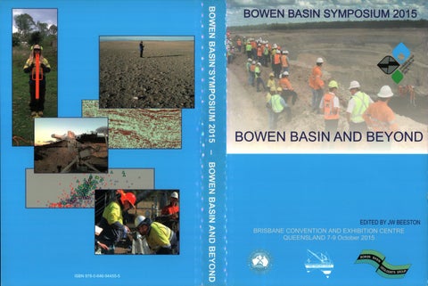
Bowen Basin Symposium 2015 - Bowen Basin and Beyond - CGG-BBGG by GSAustralia

BOWEN BASIN SYMPOSIUM 2015

BOWEN BASIN AND BEYOND

EDITED BY JW BEESTON

B·o wen· Basin Symposium 2015

Bowen Basin and Beyond

JW Beeston Editor Organised by The Bowen Basin Geologists group • and The Geological Society of Australia Incorporated Coal Geology Group Brisbane, Queensland 7-9 October 2015

Organised by: Bowen Basin Geologists Group and GSA Inc Coal Geology Group Organising Committee: POSITION

INCUMBENT

Chairman

Kirk Henderson

Secretary

Dave Edwards

Treasurer

Chris Harman

Paper, Program and Media Coordinator

Wes Nichols

Venue, Satchel and Committee Shirt Coordinator

Sylvia Michael

Proceedings Publisher/Editor

James Beeston

Workshop Coordinator

Mark Biggs

Sponsorship and Booth Coordinator

Troy Peters

Entertainment and Merchandise Coordinator

Warwick Smyth

Flyer, Presenter and AV Coordinator

Dave Kingsford

Secondary School Earth Science Event Coordinators

Wes Nichols and Sylvia Michael

Active Committee Members

Simon Brady and Bruce Anderson

Contributing Committee Member

Marko Seppanen

Representing the GSA Coal Geology Group: Dr James Beeston (Chairman/Honorary Editor, GSA Coal Geology Group) William Hayes (Vice-Chairman, GSA Coal Geology Group) Professor Joan Esterle (Honorary Secretary, GSA Coal Geology Group) Warren Hughes (Honorary Treasurer, GSA Coal Geology Group) Proceedings prepared by: JW & SA Beeston Proceedings published by: GSA Coal Geology Group (This proceedings volume is a peer-reviewed publication of the Coal Geology Group of the Geological Society of Australia Inc.) © Geological Society of Australia Inc Issued: October 2015 ISBN: 978-0-646-94455-5 Printed by: Kingswood Press Reference guides: BEESTON, J.W. (Editor): Bowen Basin Symposium 2015- Bowen Basin and Beyond. Geological Society of Australia Inc. Coal Geology Group and the Bowen Basin Geologists Group, Brisbane, October, 2015 . FERRARI, F., THOEN!, K., GIACOMINI, A. & LAMBERT, C., 2015 : A new rockfall hazard assessment methodology for open-pit coal mines. In Beeston, J.W. (Editor): Bowen Basin Symposium 2015- Bowen Basin and Beyond. Geological Society of Australia Inc. Coal Geology Group and the Bowen Basin Geologists Group, Brisbane, October, 2015, 355-362.

Contents Global Demand Anthony Williams Market evaluation ofBowen Basin thermal coals for the Indian and Chinese markets

Safety 13

Basil Beamish, David Edwards and Jan Theiler Case study of an opencut coal mine self-heating event benchmarked ag<;iinst a new laboratory test method

Coal Quality 23

Bruce Atkinson, Karryn Warren, Priyanthi Hapugoda, Graham O'Brien and Andrew Swanson Simplifying resource characterisation via coal grain analysis

Gregoire Krahenbuhl, Priyanthi Hapugoda, Karryn Warren and Graham O'Brien A new method for obtaining detailed mineral information on individual coal particles at the size that they are used in coke making

Chris McMahon Coal quality data estimations and estimators - uses and abuses

Sion Pretorius and Joan Esterle Splint coal: the hidden gremlin

Database and Modelling 51

Jared Armstrong Building value through a GIM strategy

Danique Bax Why do you keep sending my data back?

Joseph Gough Comparison ofgeotechnical logging data obtained by five different geologists over five years at Clermont Coal Mine, Queensland

Geophysics 77

Adrian Buck and Warwick Smyth The application of TSIM in defining Paleo-Channels: Case study from an active coal mine setting

Glen Guy, Alex Hossack and Maurizio Tonelli Hazard prediction in Bowen Basin dragline dumps using geophysical modelling of the coal floor

Alan Meulenbroek, Simon McMonagle, Shaun Strong, and Stewart Fletcher P- and S-wave seismic sources for ultra-shallow seismic surveying

103

Henk van Paridon Pitfalls in seismic planning in the Bowen Basin

109

Shaun Strong and Troy Peters Applications offinite-difference modelling to coal-scale seismic exp/oration

117

Shaun Strong, Steve Heam, Stewart Fletcher and John McMonagle Investigation ofproductivity enhancements for the Mini-SOSIE seismic system

123

Binzhong Zhou, Peter Hatherly and Weijia Sun Enhancing fault detection by seismic diffraction imaging

Exploration 133

Richard Barnwell 'Going off the grid ';fiexible survey designs and operational improvements made possible by cable-less recording

141

Mark Biggs Exploring for coal in lesser-known Queensland basins and reporting their resource estimates

Geology I 65

Syeda Areeba Ayaz, Joan Esterle and Mike Martin Stratigraphic architecture of the Fort Cooper and equivalent Coal Measures, Bowen Basin

171

Ben Gillam and Peter Handley Determining weathering in higher rank coal seams: Insights from South Walker Creek Coals

185

David Green and Brett Larkin Setting the standard: collecting and correcting coal borehole data

195

Guy LeBlanc Smith and Nicholas Williams Coal Resources in the Triassic Moolayember Coal Sequence: Dawson West, a new coal precinct in the Bowen Basin

211

Robert Nicoll, John McKellar, Syeda Areeba Ayaz, John Laurie, Joan Esterle, Jim Crowley, Geoff Wood, Simon Bodorkos CA-IDT/MS dating oftuffs, calibration ofpalynostratigraphy and stratigraphy of the Bowen and Galilee basins

219

Laura Phillips, Joan Esterle and Renate Sliwa Rationalising the Late Permian coal seam stratigraphy of the Koburra Trough, Galilee Basin

227

Noel Pranoto, Renate Sliwa and Justin Manalo Cockenzie: Exploring the eastern part of the Bowen Basin

235

Gordon Saul, Steven Spargo, Mike Skinner, Neil Biggs, Alan Hansen and Robert Coulls The geology of the Hyde Park coal project

Gas from coal 247

Cliff Mallett and Justin Haines

Carbon Energy underground coal gasification pilot in Queensland, Australia

Resource Quantification {JORC) 253

Monica Davis and Aaron Radonich Unreasonable prospects: What does 50 years in coal mining actually mean?

267

Brett Larkin and Gary Ballantine Classification of an example coal resource using conditional simulation

275

Craig Williams, Kirk Henderson and Spencer Summers Practical application of drill hole spacing analysis in coal resource estimation

Structural Geology 287

Peter Brooks and Scott Cutler Structural geology Daunia Mine

303

Yass-Marie Rutty Crinum North inrush and rooffailure hazard-the thalweg

Geotechnical 315

Detlef Bringemeier Prediction ofstrain-dependent permeability changes above longwall panels

329

Lachlan Campbell, David Edwards, David Noon, Pat Bellett and Nathan Ferdinands A new radar technology approach for monitoring high walls and low walls

339

Marc Elmouttie, Brett Poulsen, DeepakAdhikary, Viviana Bonilla-Sierra, Frederic-Victor Donze and Luc Scholtes Probabilistic 3-dimensional modelling of composite failure mechanisms - complicating issues and proposed solutions

355

Fredrica Ferrari, Klaus Thoeni, Anna Giacomini and Cedric Lambert A new roclifall hazard assessment methodology for open-pit coal mines

363

Sue Henderson Geomechanics of co-disposal areas

371

Kai Koosmen, John Simmons and Stephen Fityus Considerations for the design of spoil piles containing co-disposed washery wastes

383

Alison McQuillan, Ismet Canbulat, Gift Makusha and Graham Priest Implementing probabilistic designs at Anglo American Coal open cut mines

393

Terry Medhurst and Peter Hatherly The role of GSR analysis and overburden modelling in operating practice

401

Yass-Marie Rutty The evolution ofpre-driven recovery roadways at Crinum Mine

413

Ross Seedsman, Klaus Thoeni and Anna Giacomini Management of roclifall hazards at the base of a highwall

419

Ross Seedsman Kinematics ofjoint bounded blocks in development roadways and on the longwall face

429

John Simmons, Stephen Fityus, Brendan Donnelly and Andy Hammond Moisture conditions in mine spoil dumps

441

David Titberidge Determining cleat and horizontal stress azimuths using coring induced fractures in coal

453

Nicole Tucker, Jianping Li and Jody Todd Application of laboratory testing to approximate the behaviour of mixed plant rejects

Environmental Management 463

Sue Henderson and John Merritt A framework for void stability assessment within mine closure planning

473

Alan Robertson, Greg Maddocks and Ian Swane Understanding mine waste geochemistry in the Bowen Basin: from exploration to mine closure

New Technology/ACARP/R&D 481

Jonathon Ralston and Andrew Strange Towards automated mining horizon control: recent developments in radar-based real-time coal seam sensing

489

Klaus Tboeni and Anna Giacomini Determining the energy absorption capacity of safety berms in surface mining

Diamond Sponsors ARROW E ERGY has been safely and sustainably developing coal seam gas (CSG) since 2000, and began commercially supplying it from the Bowen Basin in 2004. Arrow now delivers almost 20 per cent ofQueensland's natural gas from five CSG fields in the Bowen and Surat basins, in central and southern Queensland, respectively. Arrow is owned by a joint venture company between Shell and PetroChina (50/50). Arrow operates the Moranbah Gas Project, one of the largest CSG fields in Australia, and co-owns it with AGL Energy. We also produce CSG from fields in the Surat Basin in southern Queensland and supply the Townsville (234MW), Daandine (33MW), Braemar 2 (450MW), Braemar (502MW) and Moranbah (12MW) power stations, and industrial users in Townsville and Moranbah. Our exploration tenements that cover approximately 2 I ,000km 2 across Queensland offer opportunities to support both domestic and international demand for energy.

1>))) rrOWenergy

go further

• -

bhpbilliton resourcing the future

BHP BILLITON IS PROUD TO SUPPORT THE 2015 BOWEN BASIN SYMPOSIUM BHP Billiton is a leading global resources company. With a world-class portfolio of large, long-life, low-cost, expandable, upstream assets, excellence in geoscience is critical to our exploration and resource development activities. We are among the world's largest producers of major commodities, including coal, copper, iron ore, nickel and uranium, and have substantial interests in oil and gas. Our unrivalled portfolio of high quality growth opportunities will ensure we continue to meet the changing needs of our customers and the resources demand of emerging economies at every stage of their growth. With a 130 year history and a core portfolio of 19 assets in 8 countries across 3 continents we are committed to working in ways that are true to Our BHP Billiton Charter values of Sustainability, Integrity, Respect, Performance, Simplicity and Accountability. Our corporate strategy is based on owning and operating assets diversified by commodity, geography and market. To achieve this, we also need a workforce that reflects diversity in all forms, including gender, skills, experience and ethnicity. Embracing openness, trust, teamwork, diversity and relationships that are mutually beneficial, reflects our core value of Respect and is the focus of our people strategy. In all our efforts, we aim to be inclusive and build pride and loyalty in our workforce.

ALS LIMITED (ASX:ALQ) is an ASX 100 company that provides professional testing, inspection and certification services throughout the world. ALS delivers technical services through four divisions across thirteen service lines. Minerals: Geochemistry, Metallurgy, Mine Site and Inspection Life Sciences: Environmental, Food, Pharmaceutical, Electronics and Consumer Products Energy: Coal and Oil & Gas Industrial : Asset Care and Tribology Our passionate and dedicated team of over 11,700 employees are strategically located across 350 sites in 65 countries. At this year's Bowen Basin Symposium our Coal and Oil & Gas teams will be showcasing our technical capabilities in coal, geology and coal seam gas.

ALS Coal delivers laboratory testing and analytical solutions for every stage of your coal chain. At its core is coal quality through all phases from geology thru mining, to CHPP and taking your commodity to market. For any mining company it is integral to Know Your Coal, Manage Quality and Capture Value during each stage. ALS Oil & Gas offers a complete Well to Lab solution providing well site reservoir or consistent temperature desorption services. Gas characterisation samples can be collected as directed in the field or the lab. These techniques are currently being utilised in the CSG, shale gas and fugitive emissions industries in Australia. Right Solutions x Right Partner

alsglobal.com/coal

alsglobal.com/oilandgas

Diamond Sponsors

Peabod

I II ENERGV

PEABODY ENERGY (NYSE: BTU) is the world's largest private-sector coal company and a global leader in sustainable mining and clean coal solutions. The company serves metallurgical and thermal coal customers in nearly 30 countries on six continents. Peabody's global platform reaches six continents and creates a strategic advantage. The company has approximately 9 billion tons of proven and probable coal reserves and owns, through its subsidiaries, majority interests in 28 coal operations located throughout all major U.S. coal-producing regions and in Australia. Peabody has mining operations in Queensland and New South Wales, as well as active coal trading in all major Australian coal regions through Peabody COALTRADE.

XENITH CONSULTING-AUSTRALIA'S LARGEST COAL MINING CONSULTANCY is a privately owned consultancy that provides professional mining services in the areas of geology, exploration, mine planning, business analysis, risk advisory, infrastructure and environment as well as management services in operations, contracting and investments. For over 10 years our clients have chosen us because they have challenges that only people with extensive understanding of coal mining and all its complexities can solve. Xenith aspires to become the preferred consultant to the resource industry through its unsurpassed reputation for delivering fresh, innovative solutions that provide value to our clients. Xenith provide a fully integrated service, ongoing system support and our willingness to share ideas and our strong desire to take ownership of the problem ensures solutions are tailored to the needs of our clients. We have built a solid reputation for delivering value to our clients and their businesses. Our ability to deliver on promises stems from our culture of valuing relationships; our people are paramount to our success therefore, we aim to provide a stimulating, and rewarding environment that satisfies individual needs and recognises and values individual contribution to our success. You can count on us because we really do care about the outcome, our reputation depends on it.

BRISBANE - SYDNEY - HUNTER VALLEY - SOUTH AFRICA - INDONESIA

www.xenith.com.au I E: info@xenith.com.au

VELSEIS INTEGRATED SEISMIC TECHNOLOGIES has built a reputation as the leading Australian seismic contractor with over 30 years experience throughout the Asia Pacific region, servicing the coal, petroleum and mineral industries. Velseis has an unrivalled reputation in the acquisition of high resolution seismic data utilising explosive, Mini-SOSIE and Vibroseis sources. Velseis offers a fully integrated professional service incorporating survey design, drilling and the acquisition of2D, 3D and multicomponent surveys. Complimenting these acquisition services is Velseis' processing division. Utilising advanced processing workflows, Velseis Processing is committed to providing high quality seismic services to the petroleum and mineral industries and is at the forefront of the provision of high resolution sub-surface imagery to the Australian Coal Industry. Velseis has a proactive commitment to research and development, encompassing specialised research initiatives as well as high level Geophysical support for their production divisions. Velseis' QHSE management system provides a clearly defined set of standards and procedures for quality control, health and safety and environmental management. Our operations strive for the highest technical standards with minimal risk to Velseis staff, clients and the environment. Velseis holds both ISO9001 and AS4801 certification, emphasising the company's commitment to QHSE. www.velseis.com

info@velseis.com

Welseis Integrated Seismic Technologies

Graphite Sponsors 4cansull .,

BUREAU VERITAS

Anthracite Sponsors

RioTinto

ERC ~: * : ~ Energy R•■ ource ■ Consultlng Pty Ltd

energeo GEOBRUGG••

1-)~

Bituminous Sponsors

.~ WestSide ___ ~

PRODUCTS DRILLING a MINING SUPPLIES

DRILLIOC SERVICES

n\.

NEW HOPE GROUP

A~,~~ ~p DGeology "9'" A"'b'alia Pty Ltd.

Lignite Sponsors

........ .....,...., ----

~~~ ----...-.-,~~

.;;;;;;;;;.,-~-==r

LUCAS

McE/roy Bryan G.o/oglcal Services

Ice Breakers and Supporters Geosclence Society Auslfflffl

Trade Exhibitors Geobrugg HDR Energy Resources ABC Products GroundProbe AUSIMM AIG ALS Velseis BHPBilliton Peabody Arrow Xenith QGESS Geoconsult Preplab Testing Bureau Veritas acQuire Terrex Maptek Geoimage Geos Mining Surtron PESA Sigra Datamine UQ - Earth Science Geological Solutions Geosensor Wireline GSQ SRK RGS Environmental Gap Geo Mira Geoscience ABB Enterprise Micromine Hodge Drilling Golder Associates SCT Operations Bore Hole Wireline Wireline Services Australasian Groundwater and Environmental Consultants Weatherford

Global Demand

Anthony Williams

Market evaluation of Bowen Basin thermal coals for the Indian and Chinese markets China and India imported 218Mt and 123Mt tonnes of thermal coal respectively in 2012 and this number is expected to increase over the next 5 years. Both countries have a domestic supply of coal available but, due to shortfalls in supply of domestic coals, both countries import significant quantities of coal. There is significant potential for growing the volume of Bowen Basin thermal coals sold into these markets. It is highly beneficial to coal producers of Bowen Basin coals to understand how the coal quality, utilisation performance, and value-in-use of Bowen Basin coals would be perceived in these markets. Blending of coals is also a common procedure in many power plants with Indian and Chinese plants have the options of blending imported coals with domestic coals as well as with other imported coals. The paper will explore the market potential of Bowen Basin coals for the Indian and Chinese markets. The paper will discuss coal quality of Bowen Basin coals, expected utilisation performance in coal fired power plants and the value-in-use of Bowen Basin coals from the point of view of a Chinese and Indian Power Plant. Keywords: Value-in-use, Thermal Coal Market, Thermal Coal Utilisation,

INTRODUCTION There is a significant opportunity for producers in the Bowen Basin to develop their technical marketing strategy to focus on China and India for future growth in coal exports. Figure 1 shows historical and forecast thermal coal imports of China, India, Europe, Japan, Taiwan, and South Korea as sourced from the Australian Department of Industry and Science, 2015 . China and India standout as significant coal importers over the next 5 years as seen by the predicted growth in coal imports. India is predicted to increase coal imports by 50 percent, a significant increase. Although there are efforts in India to boost domestic coal supply, it is unlikely that the growth in coal production can match the growth in demand for coal-fired electricity. Japan, Taiwan and South Korea used to be primary targets for the exports of Bowen Basin and other Australian coal but the predicted imports volumes indicates a slowly growing market in Taiwan and South Korea, and a decreasing market in Japan over the next five years. The Europe market is expected to stay relatively constant over the next five years. India currently imports 3 times as much Indonesian coal as Australian coal (IEA coal statistics, 2014) and there is consequently significant potential for Bowen Basin and Australia producers to grow market share in India.

Figure 1 also shows the predicted coal exports from the major producing countries including Indonesia, Australia, Russia, Colombia, South Africa and the United States. Indonesia is the largest exporter of coal which is expected to continue over the next five years. However, exports from Indonesia are expected to decrease by approximately 5 percent over this time period, most likely due to the increasing demand for domestic coal fired electricity within Indonesia. Coal exports from Australia and South Africa are expected to increase by 20 percent and exports from Colombia are expected to increase by an impressive 60 percent. The United States is currently a minor exporter of thermal coal which is expected to reduce over the next 5 years.

POWER PLANTS IN CHINA AND INDIA China and India are significant users of coal-fired power. Coal generates approximately 81 % of China's electricity and 71 % oflndia's electricity (IEA coal statistics, 2014). Figure 2 shows the location of power plants throughout India and China. India has power plants scattered throughout the country, and China also has plants that are scattered, but these are primarily located on the eastern side of the country. The purple dots indicate power plants that are greater than 200kms from the coastline. It is unlikely that these power plants would import coal unless a domestic supply of coal was unavailable. China and India have domestic supply of coal available and consequently the majority of power plants are designed to utilise domestic coal, although a small percentage have been designed to utilise imported coal. A significant cost for coal-importing power plants is shipping. Shipping costs can fluctuate significantly depending on market conditions. Average shipping costs from different coal exporting ports in Indonesia, Australia, Russia, Colombia, South Africa and the United States were determined from Coalspot (2005). An average cost per distance was calculated from published shipping costs for Capesize ships in costper-tonne for difference routes to China and India. Average distances were determined between the coal exporting ports of the major coal exporting countries and the ports of China and India. Shipping distances were determined using BP Marine tables and considered main shipping lanes that circumvent travelling around coastlines. Average shipping costs in $It were calculated considering the average $/distance and the actual shipping distances between the export and import ports. Figure 3 shows the costs of shipping a tonne of coal to India and China from Australia vs. other exporting countries.

Bowen Basin Symposium 2015

COAL EXPORTS

COAL IMPORTS Indonesia

400

350

-.... -.... ~

300

CII L..

China

250

Australia

Europe

........ CII 200 ~

150

---

lC~uth Korea

Japan Taiwan

2012

2014

2016

2018

Russia

2020

Colombia

L 2012

South Africa

United States

2014

2016

2018

2020

2022

Figure 1: Historical and forecast thermal coal imports and exports for major importing and exporting countries (Australian Department of Industry and Science, 2015) .

....... D

■ 0 to lOObns ■ 100 to 200bM

■ NotAppliabl<

D Noteo..t.i

........................ Figure 2: Location of operating coal fired power plants in China and India (A&B Mylec power plant database).

Global Demand Indonesia

Indonesia

Australia

Russia

Colombia

South Africa

United States

United States 0

Average Shipping Cost to India ($US/t)

Average Shipping Cost to China ($US/t)

Figure 3: Average shipping costs to India and China from major coal exporting countries.

Based on shipping rates alone, for Indian power plants, coal calorific value, moisture and ash content. Figure 4 shows sourced from Indonesia, South Africa, Australia and Russia coals with a wide range of calorific values, moisture contents are preferred over coal from Colombia and the United States. and ash contents. The benchmark price per energy unit Chinese power plants prefer coal from Indonesia, Russia and increases as the calorific value of coal increases and moisture Australia and not necessarily from Colombia and the United content decreases. This means the lower energy content coals States. Coal imports from South Africa may be acceptable. are cheaper on an energy basis and this gives credence to Shipping rates have decreased significantly from 2014 due the massive growth in coal exports from Indonesia. The data to the collapse in the oil price and, consequently, coal can is scattered for variation in ash contents. An equation was be transported further than it can at the previously higher oil , developed to estimate the price of a coal from calorific value, prices. Consequently, because of lower fuel costs, coal from ash content and moisture content. Sulfur content is also an sources such as the United States or Russia may be able to important parameter with respects to the pricing of coal, but compete in the Indian market. However,coal from the United its importance to pricing is reliant on the local SO2 emissions States and Colombia typically flow into the European market. regulations of the power plant that's purchasing the coal. Considering this market is expected to stagnant over the next Coal prices are used to determine the value-in-use metrics five years and with the expected rapid growth in coal from of different coals in a Chinese power plant and an Indian Colombia, some of this coal may end up being transported power plant. to the South-East Asia region. The evaluation in this paper The physical tests conducted in a proximate analysis are ash will focus on coal exports from the Bowen Basin and other content, moisture content and volatile matter content while regions in Australia, Indonesia, Russia and South Africa to fixed carbon is calculated by difference .. A correlation was power plants in China and India. developed between normalised fixed carbon and calorific value. The normalised fixed carbon was calculated from the Power plants are designed to a coal specification which could as-received ash and moisture contents such that: be a domestic coal or possibly an imported one e.g. Japanese power plants are designed for imported coal. Key coal quality specifications for power plant design include calorific JOO =Ash Content (%ar)+Moisture Content (%ar)+ value, ash content and moisture content. These parameters Fixed Carbon (%ar) are also extremely important in the pricing of coal as shown The developed correlation has a R2 value of 0.893 indicating in Figure 4 which compares the HBB marker published by a strong correlation exists between calorific value and the Indonesian government, adjusted for coal energy with normalised Fixed Carbon. The relationship allows the plotting

,,..,.... ----~ ...• .

G 2.5

V ). V')

:::>

........... .... ,.,,,.,...... ·1 ·. .

. -...... .

~ 1.5

....111

••

..:,J!

a:) ~

:r: 0.5 0

3000 4000

5000

6000

7000 0

Calorific Value (kcal/kg ar)

Total Moisture (%ar)

50 0

Ash Content (%ar)

Figure 4: Comparison of HBB marker (April 2015) with calorific value, moisture and ash content.

Bowen Basin Symposium 2015

in a large variation in calorific values and price. Coals from other countries are scattered around the bottom right comer.

of coals on a ternary diagram (Figure 5) with the axes of ash content, moisture and fixed carbon/calorific value. Instead of using the fixed carbon determined from the proximate analysis in the chart, the normalised fixed carbon used for the chart was calculated from the calorific value which ensures the parameter is independent of ash and moisture. A&B Mylec's coal quality database is plotted in Figure 5. The data are filtered for export thermal coals and grouped by location - Indonesia, South Africa, Russia, Other countries, Bowen Basin and other Australia. Considering that pricing is heavily dependent on energy, moisture and ash, pricing contours are also included in Figure 5.

A database of coal-fired power plants around the world has been compiled by A&B Mylec and contains a range of plant information, including design specifications for some plants. The information was sourced from commercial work library sources and other publically available sources. Whit; th information in the database is currently under review, the power plant data for India and China has already been reviewed and validated against data from multiple sources. Included in Figure 5 are the ranges of plant specifications for Chinese and Indian power plants. The design ranges include coals that have lower coal quality characteristics than that of exported coals because the plant has been designed to use local, domestic coals without any form of washing or upgrading process. Indian coals are known to have very high ash and the specifications indicate that the power utilities can utilise ash contents up around 45%. India does also have high moisture content coal resources which explains why the plant specifications have high moisture limits.

Figure 5 shows that all coals tend to be localised within the lower right comer of the ternary diagram and have high energy, an ash content less than 50% and moisture levels less than 50%. Most exported coals have superior properties than coals used domestically (the exception being Indonesia. Most of the Bowen Basin coals are priced above $50/t with ash contents less than 20%, moisture less than 15% and calorific values greater than 6000 kcal/kg. The Indonesian coals are grouped along the base of the diagram and have low ash content and a high variation in moisture content that results Indonesia •

South Africa

•

Other

•

Other Australia

•

Bowen Basin

Ash Content (% ar)

- - - Price Contours - - India Plant Range - - China Plant Range

Moisture (% ar)

I I

,' I

♦/

♦♦ •

•

♦

I I

♦

■

■ ••

■I '

Fixed Carbon (%ar) 943

4790

8550

Calorific Value (kcal/kg ar) Figure 5_: Comparison of calorific value, ash content, and moisture for Bowen Basin coals with other Australian and Internatwnal coals.

Global Demand A small selection of Indian coals are included in Figure 5 under the 'Other' category. However these coals do not reflect how low the quality of product coal can be in India. Coal oflndia, the major coal producing company in India, sells domestic coal with energy contents down to 2200kcal/kg (Coal of India website, 2015)

The evaluation of the impact of coal properties on plant performance assesses whether a particular coal will, or will not, suffer any extraordinary cost penalties due to any of the following issues: •

Even though the product specifications for Bowen Basin coals and other traded coals exceed the typical plant specification of Chinese and Indian plants, they may still be used by the power plants in a blend or utilised as 100% feedstock, assuming that some validation testwork is performed to ensure the plant can safely use the coal.

IMPACT-THERMAL VALUE-INUSE MODEL The research in this paper will use a value-in-use model called IMPACT-Thermal to predict utilisation performance and value-in-use metrics of a coal fired power station in China and India. There have been numerous publications describing and utilising the model and further details ofIMPACTThermal can be found in these publications (Juniper, L 1996 and Juniper & Pohl, 1999).The outputs from IMPACTThermal were reviewed and evaluated using MarketMastor™, a tool created to facilitate the evaluation of market data and information by utilising value-in-use models, correlations and data from coal quality specifications, power plants, cement plants, steelworks and shipping ports. The assumptions are that the coal will be delivered to a modem super-critical 300 MWe, pulverised coal-fired power plant located: 1.

on the Eastern coast of India; and

in Hong Kong, China.

The general power plant operating conditions assumed are set out in Table 1.

•

Load limitations caused by exceeding operating limits, such as: o

Exceeding dust or pollutant emissions;

Exceeding pulveriser or boiler operating limits;

Not attaining required steam conditions;Boiler shutdown or loss of availability caused by excessive ash deposition; and

High carbon-in-ash levels, which would prevent sale of fly ash to the cement industry.

IMPACT-Thermal accounts for all of the above limitations with the exception of steam temperature attainment. The mass and energy calculations required to estimate this aspect are very complex and not available in IMPACT-Thermal.

Power Station Costs and Fuel Costs The performance and costs for individual components in the power station's coal chain can be estimated by using indices and/or correlations between coal properties and plant performance, which have been developed over the past few years. Costs of operating the various components can then be evaluated by assigning relative costs to the variations in performance for a range of coals of interest. This procedure provides an evaluation of the overall cost benefit of using a particular coal in pulverised-coal-fired (PF) plant, and a relative value of the coal of interest, compared to a range of competing coals. Fuel costs include the net cost of the coal as delivered to the power station stockyard. The price to the stockyard includes the freight cost and a discharge handling cost.

Table 1: Assumed Power Plant Parameters for Chinese and Indian plants. .,. '':. ' Location Capacity Annual Capacity Factor Turbine Heat Rate

·"'

.lflilli, .. MWe MJ/MWh

~. . . .

.. ':,

a.;.--.:.; ~

·,

:,:

Hong Kong 350MWe 90 8300

East Coast 300MWe 85 9000

Base 20.0 130 Verticle spindle 6 30 50 70

Electrostatic Precipitators No Yes

Boiler

Loading Profile Excess Air Flue gas exit temperature Mill type Number of pulverisers Pulveriser capacity Design HGI Design PF fineness

% oc

%<75mm

Environment

Dust Collection Flue Gas Desulphurisation Fly ash utilisation

Bowen Basin Symposium 2015

UTILISATION PERFORMANCE OF BOWEN BASIN COALS

The Bowen Basin coals are expected to require lower power consumption in their utilistation than coals from key competing countries like Indonesia, South Africa and Russia.

Four parameters were evaluated for utilisation performance including: power consumption, mill wear, ash deposition potential and carbon-in-ash. Various statistics are used to assess the utilisation performance and allow comparison between different countries. The statistics include the median, 1st quartile, 3rd quartile, 5 percentile and 95 percentile which are described in Figure 6. Figure 7 shows the statistics for the expected utilisation performance for the major thermal coal exporting countries, major thermal coal importing countries that also have a domestic supply of thermal coal available, and coal exporting regions within Australia. The top exporting countries include Indonesia, Australia, Russia, Colombia, South Africa, and the United States of America. The major importing countries include India and China. The coal exporting regions in Australia include the Bowen Basin, other QLD, Hunter Valley and other NSW.

Mill wear

95 Percentile

Median

5 Percentile

\ I

1st Quartile

3rd Quartile

Figure 6: Description of bars used in figures.

A factor that significantly contributes to the cost of pulverising is the wear of mill components. Wear is generally governed by the combined influence of coal properties, mill operating conditions and the materials that make up the grinding components. Coals with a high concentration of hard minerals (mainly quartz), are likely to cause higher mill wear rates. Quartz content can be estimated from the silica and alumina contents of the coal ash. Coals that have quartz content in their entrained mineralsof less than about 3--4% are unlikely to cause unacceptable wear of mill components. Figure 7 shows that Bowen Basin coals have low levels of quartz (which should result in low levels of mill wear). Their mill wear levels are lower than coals from other Australian regions and similar to coals from South Africa and the United States. As a result of their low ash contents, Indonesian coalshave quartz levels significantly less than Bowen Basin coals. The quartz levels in Bowen Basin coals are significantly less than that found in domestic Indian coals and, consequently, Indian power plants will achieve reduced pulverising costs when using Bowen Basin coals. The quartz levels in Bowen Basin coals are are similar to Chinese coals and, consequently, Chinese power plants should notice little variation in mill wear behaviour when utilising Bowen Basin coals.

Mill power consumption The coal property most commonly used for evaluation of grinding performance by utilities is HGI. The consequence of low HGI values on the grinding performance of coals is: a) a coarser product which may result in poor burnout, and b) higher power consumption to produce a product of the required fineness. Mills are designed to handle the coal throughput necessary for a given boiler size and the energy content of the coal. A plant fired on low-energy content coals would be expected to have a higher pulverising capacity than a power plant designed to handle a bigh-nergy coal. For example, an Indian power plant using low-energy domestic coal would be expected to have a higher pulverising capacity than a Japanese plant utilising a high-energy Newcastle coal. Consequently, the Indian plants and some of the Chinese plants would be expected to have spare mill capacity when utili sing higher energy coal. Figure 7 shows expected power consumption (adjusted for coal energy). Bowen Basin coals require very low power consumption when compared to coals from other Australian regions and low consumption when compared to other countries. This is due to the relatively high HGI and calorific value of Bowen Basin coals. However, as well as between Bowen Basin coals and other Australian coals, there is a wide range of variation in these coal quality parametersbetween Bowen Basin Coals themselves, This indicates that individual Bowen Basin coals should be evaluated independently.

Boiler tube erosion is also affected by quartz levels in coal and, therefore, coals with a high concentration of bard minerals are likely to cause high rates of boiler tube erosion. Erosion is governed by the combined influence of coal properties, boiler flue gas conditions and tube materials. It is important to appreciate that the size of the quartz particles is a key factor and no assessment of the quartz particle size has been performed in this study. Work by Raask (1985) and Bauver and others (1984) bas shown that quartz particles above a certain particle size are very influential in the erosion process. Concentrations of quartz above 6 percent in coal have been shown to cause erosion problems in boilers. The levels of quartz in Bowen Basin coals are less than 6 percent and consequently should cause minimal erosion problems.

Slagging Ash deposition (slagging and fouling) causes problems in boilers by impeding the heat transfer to the water and steam tubes in the boiler. Operating cost penalties can arise for several reasons, including reductions in heat transfer resulting in reduced load, shutdown of the boiler to remove deposits, and removal of deposits by soot blowers requires the use of non-recoverable steam. Shutting down a boiler to remove slagging deposits can result in loss of revenue in the order of millions of dollars. The propensity of a coal to cause slagging problems in full-scale boiler plant is also affected by the

Global Demand Exportlnc Countries

Exportlnc Countries

Indonesia Australia Russia Colombia South Africa USA

lmportinc Countrlas

lmportlnc CountriH

China India

Australian R•cions

Australian Rqions

Bowen Basin Other QLD Hunter Valley Other NSW

World

World 0.2

0.6

0.4

0.8

Quartz (% In coal)

Mill Power Consumption (kWh/GJ)

-=-=-=-==--==============:::::: ~===========--------!lmi:i::::J Exportlnc CountriH

Exportlnc Countrias

Indonesia Australia Russia Colombia South Africa USA

lmportinc CountriH

lmportinc Countries

China India

Australian R•cions

Australian R■cions

Bowen Basin Other QLD Hunter Valley Other NSW

Bowen Basin Other QLD Hunter Valley OtherNSW

World

World 0

Carbon in Ash (%)

Overall Slagging

Figure 7: Utilisation performance metrics for Mill Power Consumption, Quartz in coal (mill wear), Overall slagging assessment and Carbon in Ash for Bowen Basin coals and other countries and regions. boiler design, operating conditions and coal properties. Ash fusion temperatures and ash deposition indices based on ash chemistry are often used for evaluating the ash deposition characteristics of coals. Figure 7 shows an overall rating for ash deposition propensity for Bowen Basin coals and other traded coals. The overall rating is based on a weighted average of the individual indices, with the weighting decreasing from top to bottom of the table. Overall slagging numbers greater than 10 indicate severe slagging potential, numbers greater than 5 and less than 10 indicate moderate potential, and numbers less than 5 indicate low potential. Bowen Basin coals are expected to have moderate propensity for ash deposition. This propensity is both higher than coals from other regions in Australia and higher than coals from Indonesian, United States and China. Their propensity is similar to competitor coals from Russia, Colombia, and South Africa. The results indicate Bowen Basin coals should behave similar to domestic Indian coals, which should make the coals acceptable to Indian power plants. Bowen Basin coals are significantly superior (have lower propoesnity for slagging)

to Chinese coals and consequently Chinese power plants will find these characteristic appealing.

Carbon in ash The main impact on performance and cost due to combustion characteristics comes from the burnout efficiency of coal. This not only affects boiler efficiency, but it also aids the potential for fly ash to be sold as a by-product to the cement industry. Fly ash can be sold to the cement industry to be used as an additive to cement, provided that the residual carbonin-ash content is less than 5% (depending on location) and the colour of the ash is acceptable. Ash with high carbonin-ash values will cause problems with the cement product. However, the actual limit may vary at different plants. Estimates of pulverised coal burnout can be made from correlations, including adjustments for the effect of pulverised coal size distribution. Fly ash utilisation rates are estimated

Bowen Basin Symposium 2015

at approximately 67 percent for China and 14 percent for India in 2010 (Heidrich & others, 2013). The primary factors that indicate whether a power plant can sell fly ash or not depends on whether the fly ash satisfies the customer's plant requirements and the plant's proximity to its supplier. MarketMastor™ has a database of worldwide cement plants and, considering the distance to the closest cement plant can be determined for every power plant in the world, a good approximation can be made whether these plants are likely to utilise fly ash or not. Chinese and Indian power plants both have accessible cement plants available to use the fly ash, albeit with a sale price of $0/t. Giving away fly ash is still economically appealing for power plants as it avoids fly ash disposal costs. Figure 7 shows that the expected carbon-in-ash for most Bowen Basin coals is above 5 percent, which is similar to the world average and similar to coal from other coal exporting countries. The carbon-in-ash content is slightly higher for coals from SW and significantly higher than coals from other Queensland basins. This includes some of the high volatile, reactive coals from the Surat Basin. There is a broad range of results indicating the analysis should be performed on individual coals. Domestic Chinese coals typically have slightly lower carbon-in-ash than Bowen Basin coals. The carbon-in-ash content is higher for Bowen Basin coals than that typically found in for domestic Indian coals which have low carbon-in-ash due to their high ash contents.

ENVIRONMENTAL PERFORMANCE OF BOWEN BASIN COALS In Figure 8, emissions of dust and SO 2 are compared for coals from the Bowen Basin, other Australian and coals from other countries.

Dust Emissions The emissions of dust from coal-fired power plants affects human health and causes smog. The author is unaware of any power plant in the world without some form of dust collection system installed. Modem dust collection units such as electrostatic precipitators (ESPs) and fabric filters remove the majority of dust but the emission of fine dust can especially cause health problems. The predicted dust emissions from a typical ESP installation are shown in Figure 8. Typical industry limits on dust emissions vary from country to country and from plant to plant. Typically, if dust emissions were to exceed statutory limits, then the output from the plant would need to be reduced. This would have a significant on costs because of the resultant reduction in power sold into the commercial market. In addition, there may be cause to actually import power (usually at higher cost) to fulfil contracts for power supply. Note that, where FGD plant is installed, the ESP performance becomes less critical as a large percentage of the dust is removed by the FGD sprays. Dust emissions are low for Bowen Basin coals as compared to other Australian coals and to South African coals. The emissions are similar to Russian coals and higher than coals from Indonesia, Colombia and the United States. The emissions are expected to be significantly less than domestic

EllportincCountrin

Indonesia

Australia Russia Colombia South Africa USA lmpofti• Countrin

Exportinc Countrin

Indonesia

Australia Russia Colombia South Africa USA Impart!. Countrin

China India Australian Rep,ns Bowen Basin Other QLD Hunter Valley Other NSW

Australian Rep,ns Bowen Basin Other QLD Hunter Valley OtherNSW

Wortd

China India

World

World 0

500

1000 1500 2000 2500 3000

S02 Emissions (mg/N~)

500

1000

1500

Dust Emissions (mg/Nm3)

Figure 8: Predicted environmental metrics for SO 2 emissions and dust emissions for Bowen Basin coals and other countries and regions.

Global Demand Indian coals which have high emissions due to their high ash contents.

VALUE IN USE OF BOWEN BASIN COALS

SO 2 Emissions

The cost of electricity generation at a power plant in China and India was calculated using Bowen Basin coals, coals from other regions in Australia and coals from competitor countries. The cost of utilising coal for pulverised coal fired power generation is dependent on coal properties to the extent that they impact on operating and maintenance costs, net power generated, fuel costs and waste disposal costs. The total generation costs for all the coals included the following parameters:

The emissions of SO2 are regulated by countries around the world due to its effect on human health and influence on the formation of acid rain. During combustion, coal sulfur can either be converted to SO 2 and a small amount of SO3 or the sulphur can be absorbed into the fly ash. The extent to which the sulfur is absorbed into the fly ash is dependent on the chemical reactions between sulfur and the elements in the ash, particularly calcium. The SO2 emissions relate very strongly to the sulfur content of the coal. Figure 8 shows that Bowen Basin coals have lower SO2 emissions than other coals from QLD, and that they have similar SO 2 emissions to coals from NSW. The emissions for Bowen Basin coals are lower than those from typical coals from Indonesia, Colombia, South Africa and the United States and higher than coals from Russia. Their emissions are significantly higher than those of domestic Chinese coals, which might be seen as problematic in some Chinese power plants, especially as the Chinese government reduces the emissions limits for air pollutants. The SO2 emissions for Bowen Basin coals are significantly less than domestic Indian coals which will be an important characteristic as India reduces limits for SO2 emission.

•

Base FOB coal prices were calculated for each coal from a correlation requiring calorific value, ash content, moisture and sulfur content as derived from HBB benchmark data for April 2015.

•

Ocean freight rates and discharge costs.

•

Penalties due to high carbon-in-ash values, lost income due to low load operation from limits on pulveriser capacity, and reduction in capacity factor due to ash deposition.

Figure 9 compares power plant costs with fuel costs for Bowen Basin coals and other traded coals. The fuel costs for Bowen Basin coals includes the coal cost and their transport costs normalised to the electricity generated from the plant per year. To simplify the charts, coals are categorized into 5 groups; Indonesia, South Africa, Other Countries, Other Australia and Bowen Basin. Plant costs includes capital costs, operating and maintenance costs and lost revenue costs. The plant and fuel costs are normalised to the standard output from the power plant. Preferred coals(i.e. coals with the INDIAN POWER PLANT e

CHINA POWER PLANT

••

• ••

... 35

.J:.

•

t! 25

•

t; 20

a:"'

•

15 10

Fuel Costs ($/MWhr)

■ Indonesia ■ South Africa • Other • Other Australia ♦ Bowen Basin • Russia

Figure 9: Comparison ofplant costs with fael costs for a Chinese and Indian power plant for Bowen Basin coals and other traded coals.

Bowen Basin Symposium 2015

lowest costs) are those located in the bottom left hand regions of the graphs in Figure 9.

constant, with the majority of coal lying within a narrowlydefined band.

The fuel costs for Bowen Basin coal range around $30/MWhr for the Chinese plant and $35/MWhr for the Indian plant. These costs are in the middle of the cost range for reference coals and similar to the costs for other coals from Australia. The Chinese plant is located slightly further away from Bowen Basin ports than the Indian coal port. The plant costs are low and are similar to competing coal exports. There are a significant number of competing products that have lower fuel costs but have similar plant costs. There are several products with plant costs greater than $15/MWhr that perform significantly worse than other coals. Typically, these coals result in a lower fuel cost than the other coals, but they cause some form of capacity limitation or lost revenue scenario for the power plant. The results indicate Bowen Basin have average fuel costs, but provide low plant costs which should be attractive from a Chinese and Indian power plant point of view.

The expected generation costs for the different Bowen Basin coals is similar for both the Chinese and the Indian plant, with the generation costs approximately $10/MWh higher for the Indian plant. The bulk of the coals lie in defined bands for both of these plants. Although the difference in generation costs between the top and bottom of these bands may only be approximately $10/MWhr, this difference equates to $26 million per year for the Chinese plant and $28 million for the Indian plant. Consequently, these plants will experience a significant reduction in costs if a coal is selected fromk the bottom of the range. The Bowen Basin coals lie in the middle of this range and, consequently, power plants in China and India can purchase better performing coals from other countries.

A comparison of total generation cost versus the delivered cost of coal for Bowen Basin coals and competitor coals is given in Figure 10. The delivered costs refers to the coal price plus shipping price. Other costs such as port and handling costs are not included. The delivery cost of Bowen Basin coals to the Chinese plant or Indian plant varies between approximately $60/t to $90/t. This is a significant cost variation and it is due to the varying properties of the coal products. The delivery costs are higher than for Indonesian coals and they are similar to South African and other Australian coals. Indonesian coals are popular in the market due to the low price and proximity to the major markets in South-East Asia. It could be expected that the cheaper coal price of Indonesian coals would result in lower generation costs.Yet, Figure 10 shows generation costs remain relatively

If delivered costs are evaluated considering the electrical output from a plant, a different relationship is observed between Generation Cost and delivered cost ($/MWh) as shown in Figure 11. A clear relationship is observed where increased generation cost results in a an increased delivered cost per electrical output increases. Although Bowen Basin coals are not located at the lower end of generation cost, they are positioned around the average of the dataset. The Bowen Basin coals have a lower delivered cost than South African coals into the Chinese market. However, the South African coals tended to be slightly better than Bowen Basin coals for the Indian power plant. The Bowen Basin coals performed similarly to other Australian coals. Indonesian coals tend to have low generation and delivered cost.

The complexity of coal selection is magnified when coal blending is considered. Domestic Chinese and Indian coals

CHINA POWER PLANT

INDIAN POWER PLANT

•

••

•

• ••

••

•$28M/y,

••

•

1•$26M/y,

•

30 0

Delivered Cost ($US/t) Indonesia

100 0

Delivered Cost ($US/t) South Africa

other • other Australia ♦ Bowen Basin • Russia

Figure 10 Comparison of total generation costs with delivered cost of coal (coal price + shipping costs) for a Chinese and Indian power plant for Bowen Basin coals and other traded coals.

100

Global Demand 90

CHINA POWER PLANT

INDIAN POWER PLANT

•

:c 70

•

-... ~

"' 60

••

·.;::;

•

C QI

...

iii ~ 40

---•.•

•$28M/y,

,_,.

I!]

••

• •

:. •

=$26M/yr

• •

30 20

-,--

Fuel Costs ($/MWhr) Indonesia ■ South Africa

'35

Fuel Costs ($/MWhr) Other • Other Australia • Bowen Basin • Russia

Figure 11: Comparison ofgeneration costs and delivered foe! costs in $/MWh for Bowen Basin coals and other traded coals. may be blended with imported coals with the objective of optimising generation and maintaining stable production.

CONCLUSIONS Selection of coal by a power plant is a complex process. Although some coals may have lower delivered prices than other coals, this may not translate to lower overall generation costs. Coals with the same delivered cost can have widely different effects on generation costs and millions of dollars can be wasted utilising poorly performing coals. The research in this study has identified that Bowen Basin coals have: •

Low mill power consumption as compared with other Australian coals and key competitor countries (Indonesia, Russia and South Africa) for the Chinese and Indian markets.

•

Low potential for mill wear and erosion as compared with other Australia coals and Russian coals, they are similar potential to South Africa coals and higher potenmtial for mill wear than Indonesian coals (due to low ash content).

•

• •

Moderate propensity for ash deposition (which is higher than that for other Australian coals), similar depositon propensity to South Africana and Russian coals and less slagging propensity than Indonesian coals. Slightly higher carbon-in-ash than NSW coals but similar carbon-in-ash to coals from competing countries. Low dust emissions as compared to other Australian coal and South African coals, similar to Russian coals and higher dust emissions than coals from Indonesia.

•

Similar SO 2 emissions to NSW and lower emissions than coals from Indonesia, South Africa, but SO2 higher emission than coals from Russia.

Bowen Basin coals are an acceptable source of coal for power plants in China and India. However, they are not the cheapest coals available and their delivered costs were around the median price ofreference coals. Cheaper coals are available that can also achieve lower generation cost, but these coals can only supply so much of these rapidly growing markets. Some of the results for Bowen Basin coals were broadly spread and, consequently, further evaluation should be performed on individual coals. Blending is also performed at a growing number of power plants and, consequently, more in-depth evaluations are required into the blending of individual Bowen Basin products with domestic coals and other coals from other countries.

REFERENCES AUSTRALIAN DEPARTMENT OF INDUSTRY AND SCIENCE, 2015: Thermal coal outlook, March 2015 Commodity Data, , http://www.industry.gov.au/industry/Office-of-the-ChiefEconomist/Publications/Pages/Resources-and-energy-guarterly. aspx, Accessed 5 May 2015 BAUVER, W.P., BIANCA, J.D. & FISHBURN, J.D., 1984: Characterization of erosion of heat transfer tubes in coal fired power plants. ASME Paper 84-JPGC-F4-3, New York, NY, USA, American Society of Mechanical Engineers, vp (1984). COAL INDIA LIMITED, 2015: Website - https://www.coalindia .i n/ en-us/ourbusiness/productsservices.aspx, accessed 8 May 2015, Gross calorific value bands on non coking coal produced by Coal of India. COALSPOT.COM, 2005: Capesize Freight Rate Matrix, http://www. coalspot.com/shipping/capesize.php, Accessed April 2005.

Bowen Basin Symposium 2015

HBB MARKER, 2015: Indonesia coal price reference (April 2015). HEIDRICH, C., FEUERBORN, H.J. & WEIR, A., 2013: Coal Combustion Products: A global prospective. 2013 World of Coal Ash (WOCA) Conference, April 22-25, Lexington, United States. IEA STATISTICS, 2014: Coal Information 2014, International Energy Agency, 2014. JUNIPER, L.A., 1999: Thermal Coal Technology-A manual for Australian coal. QTherm Program, Queensland Department of Mines and Energy. JUNIPER, L.A. & POHL, J.H., 1996: Impact of Coal Properties on Power Generation Costs. Workshop on Impact of Coal Quality on Thermal Coal Utilisation, CRC for Black Coal Utilisation, Brisbane. RAASK, E., 1985: Mineral impurities in coal combustion behaviour, problems and remedial measures. London, UK, Hemisphere Publishing.

Anthony Williams A&B Mylec Pty Ltd, 146 Leichhardt St, Spring Hill, QLD 4000, Anthony.williams@abmylec.com.au, Ph +6174931 0980, +61427910 049

Safety

Basil Beamish, David Edwards and Jan Theiler

Case study of an opencut coal mine self-heating event benchmarked against a new laboratory test method As rare cases of spontaneous combustion have previously been recorded at Meandu Mine, a study was commissioned by site personnel in early 2014 as part of due diligence for thermal coal stockpile management at both Meandu and the Tarong Power Station. Under managed stockpile conditions the coal was assessed to have limited capacity to achieve thermal runaway. During the final reporting of the initial study an in-pit spontaneous combustion event was reported at Meandu Mine. This outcome shows that under specific site conditions and given sufficient time, particular Meandu coal seam plies may be prone to spontaneous combustion. The event also provides an ideal opportunity to benchmark existing laboratory spontaneous combustion test methods against a recorded in-pit spontaneous combustion event. Results from a new test method indicate an incubation period that closely matched the actual reported heating event at Meandu Mine. This case study provides a valuable comparison for future mining development at Meandu and for other mines as well. Keywords: Spontaneous combustion, Meandu Mine, opencut, thermal coal, adiabatic testing, thermal runaway)

INTRODUCTION Leading practice in all coal mines requires the implementation of a Principal Hazard Management Plan (PHMP) for spontaneous combustion. In Australia, sound scientific data is a mandatory requirement for use as a basis to assess the propensity of coal to spontaneously combust. This information is routinely used for developing risk assessments, control measures, procedures and management strategies in order to provide safer working environments for personnel, reduced potential for lost time and decrease asset losses. Australian coal mine operations have been using adiabatic oven testing since the early 1980s to rate the propensity of coal to spontaneously combust (Humphrey & others, 1981).The R70 initial self-heating rate parameter normally obtained from these tests is rated using a relative scale (Beamish & Beamish, 2012). Assessment of the resulting intrinsic spontaneous combustion propensity rating enables an appraisal of the possible risk of a spontaneous combustion event to be made: however it provides no indication of the timeframe in which an event can occur. More recent developments in adiabatic testing methods have been used to benchmark the time taken for coal to reach thermal runaway by comparing laboratory performance against actual on-site

spontaneous combustion events of a range of coals from Australia and overseas covering the full rank spectrum from low to high rank (Beamish & Beamish 2010, 2011, 2012). In response to previous infrequent spontaneous combustion events, a study was commi'ssioned as part of due diligence by site personnel and undertaken in early 2014 to assess the spontaneous combustion propensity of samples from the K4E pit at Meandu Mine. As the study neared completion, a rare in-pit spontaneous combustion event was identified and reported on-site. This paper presents the benchmarking laboratory adiabatic test results compared against the in-pit spontaneous combustion event at Meandu Mine that provides valuable information for future spontaneous combustion management planning at Meandu, which may also be applied to other coal mine operations. The experience gained from managing the event is also presented for future reference.

MINE LOCATION AND GEOLOGICAL SETTING Meandu Coal Mine is located in the late Triassic Age (- 200220 Ma) Tarong Basin approximately 200 km north-west of Brisbane, Queensland (Figure 1). A thermal product coal is produced from three main seams in the Tarong Beds to supply Stanwell Corporation 's Tarong Power Station (TPS) (Simmons & others, 2013). The Tarong Beds coal measures consist of thick coal seams which are interlayered with fine grained clay, quartz-rich or iron-rich stone bands of variable thickness within a sedimentary package of conglomerates, sandstones, siltstones and mudstone. Pegrem (1995) previously classified the coal from the Tarong Beds as high ash, low volatile, low sulphur steaming coal with weak coking properties. The seams increase in ash content with stratigraphic depth (Young, 2013). As the coal at Meandu Mine is not able to be easily ' free dug', it is blasted in order for it to be mined.

COAL SAMPLES AND ADIABATIC TESTING Coal samples representing both low and high ash content plies of the King Seam from K4E pit at Meandu Mine were tested in an adiabatic oven to establish their R70 values and to benchmark the time taken to reach thermal runaway under mine site conditions. The R70 testing procedure is described

Bowen Basin Symposium 2015

aryborough

unioon

Tarong Basin ~

SW Yanaman

••

Operating mine Mine under construction Deposit Township

__,,. Railway

__, Proposed Railway

-..... Coal export terminal 90 OOOdwt (maximum vessel size)

150°

New

152"

South

Wales j

Figure 1: Tarong Basin location (Queensland Department of Mines and Energy, 2013).

by Beamish (2005) and essentially involves testing a dried, crushed coal sample under adiabatic conditions from a fixed starting temperature of 40 °C. The benchmarking procedure, known as SponComSIM™ testing, uses the coal in its asmined moisture state and a starting temperature that reflects the site-specific conditions. The results obtained provide both an indication of the time taken to reach thermal runaway (incubation period) and the characteristic behaviour of the coal as self-heating progresses. This can be benchmarked against case history coals of known self-heating behaviour.

The coal quality details of the samples are contained in Table 1 and their similarity in coal rank is demonstrated on a Suggate rank plot (Suggate, 2000) shown in Figure 2. According to the ASTM coal rank classification the coal is high volatile B bituminous. The coal type is predominantly high in vitrinite as both samples plot within the New Zealand coal band (Figure 2).

Table 1: Coal quality data for coal samples from K4E pit Sample

K4E Low Ash K4E High Ash

Moisture content (%, ar)

Ash content {%, db)

Sulphur content (%, db)

Volatile matter (%, dmmf)

Calorific value (Btu/lb, mmmf)

ASTM rank

{°C/h)

2.74 1.39

7.3 4.9

7.4 37.0

0.31 0.23

39.1 38.3

13734 13698

hvBb hvBb

Safety ao --------~-----,------r-----r---,---,---,-- -----,------,-------;---7

0 l......----r-~~...;::_j---r-~......l-----r-.-+-~--1-~~+-,---r-~+...---r----r-+--.- ~---.---,f-,-~--.-t--r-~-.-+~--r-.-+-~.........--; 10000 10500 11000 11500 12000 12500 13000 13500 14000 14500 15000 15500 16000 16500

Calorific Value (Btu/lb, dmmsf) + K4E Low Ash

X K4E High Ash

Figure 2: Suggate rank plot of coal samples used in adiabatic testing.

ADIABATIC SELF-HEATING RESULTS AND DISCUSSION R70 values The R70 self-heating rate curves for both samples are shown in Figure 3. The R70 values range from 1.39 °C/h (high ash content sample) to 2.74 °C/h (low ash content sample), which rates these samples as having a medium to high intrinsic spontaneous combustion propensity for Queensland conditions (Beamish & Beamish, 2012). The decrease in R70 value for the high ash content samp le is consistent with the heat sink effect associated with the presence of non-reactive mineral matter in the coal (Beamish & Blazak, 2005 ; Beamish & Arisoy, 2008). The more reactive low ash content coal is therefore considered the most likely to create a spontaneous combustion event.

Self-heating performance The SponComSIM™ test results for the low ash content coal ply are shown in Figure 4. Self-heating occurs gradually from an ambient start temperature of 35 °C, with accelerated temperature increase occurring above 70 °C. Despite having a moisture content of7.3%, the self-heating rate curve does not show any rate decrease from moisture evaporation, which is clearly present for the low rank sub-bituminous Kideco coal and the high volatile B bituminous Spring Creek coal. This shows that the moisture present in the Meandu coal has only a minor moderating effect on the self-heating to thermal runaway and indicates the final surge to thermal runaway in-pit can be quite rapid. This was also observed for

the spontaneous combustion event recorded in the Meandu Mine K4E coal pit that is described in this paper. The coal stockpiled in the pit went from smouldering to an open flame within 24 hours. The Kideco and Spring Creek benchmark coals shown in Figure 4 have recorded the development of spontaneous combustion events in a period of 1-2 weeks and 6-8 weeks respectively. An empirical extrapolation from the performance of these two benchmark coals would suggest a minimum incubation period (under ideal conditions) of 10-14 weeks for the Meandu coal to develop a spontaneous combustion event. The recorded event for the K4E pit occurred in a timeframe of approximately 16 weeks. Therefore, the laboratory benchmark extrapolation produced a value that is reasonably realistic for the circumstances present at the mine, where some heat dissipation may have contributed to delaying the time to thermal runaway.

MINESITE HEATING EVENT On-site experience at Meandu Mine Spontaneous combustion incidents are rare at Meandu Mine. A recent 2014 in-pit spontaneous combustion event in the K4E Strip 12 Ace-King Seam coal confirmed the results generated from laboratory testing of the same coal seam material from that pit. At the time of the self-heating event at Meandu the K4E pit coal was being recovered from the Ace and King seam plies with a combined thickness of approximately 16 m. The coal from this pit had been utilised as 'back-up' coal during the previous wet season when access to other pits was limited. Several hundred thousand tonnes of

Bowen Basin Symposium 2015

16 160 140

-00

120

f::::s 100

-... ns

60 40 20 0

20 Time (hours)

..... K4E Low Ash

K4E High Ash

Figure 3: Adiabatic self-heating curves for low and high ash content King Seam samples from Meandu K4E pit.

160 140

-... -... 00

::::s

120 100

E ~

80 60 40 20 0

Kideco

70 80 60 Time (hours)

Spring Creek

100

11 0 120

130 140

-e- K4E Low Ash

Figure 4: Adiabatic self-heating curves for low ash content coal from Meandu K4E pit compared against self-heating behaviour of benchmark coals. blasted Ace-King coal had been retained in-pit following a mass coal blast on the 20th January 2014. The remnant coal was left exposed in-pit for approximately 120 days before a spontaneous combustion event was reported on the 19th May 2014. Following the initial report of smouldering from the exposed coal as shown in Figure 5, conditions changed rapidly with flames being reported within 24 hours on the 20th May 2014 as shown in Figure 6. Several factors were identified as triggering the in-pit spontaneous combustion event. The initial coal blast

occurred during an extended period of hot weather. The daily maximum temperature recorded on the day of the blast was 37.1 °C followed by several days of38°C and above (Bureau of Meteorology, 2014 Kingaroy Airport Daily Maximum temperature records). The elevated summer temperatures then extended for several weeks into February 2014. The coal itself was located on an elevated bench facilitating the movement of air through the blasted coal. As the coal was blasted this increased the surface area available to interact with the air. Prior to the ignition event the prevailing wind direction was noted as being from the west / south-west enabling the

Safety

19/05/2014- 08:00AM Day Shift- Smouldering - King Seam (Looking East)

Figure 5: 19/05/2014- 08:00AM Day Shift - Spontaneous combustion event recorded in Meandu K4E pit.

20/05/2014 - 07:15AM Day Shift- Full Ignition - King Seam (Looking East) Figure 6: 20/05/2014 - 07: l 5AM Day Shift - Spontaneous combustion event recorded in Meandu K4E pit. air to enter the elevated coal bench at the base of the seam and circulate through the exposed coal creating a chimney effect once the coal had begun to heat up (Figure 7). This in addition to the blasted coal creating an open pile porosity and permeability (Figure 8) combined with being exposed in-pit for approximately 120 days provided ideal conditions for a

spontaneous combustion event to develop. Although pyrite is present within the coal as visible coatings on cleat and fracture surfaces (Figure 9) it was found to be non-reactive and therefore did little to accelerate the self-heating process in this case.

Bowen Basin Symposium 2015

SCALE(m)

Figure 7: 20/05/2014 - -JJ:30AM- K4E ST12-King Coal Seam -closer view offire on edge of coal ramp looking ENE (showing chimney effect created by prevailing wind blowing front on to broken coal pile).

SCALE(m)

Figure 8: 20/05/2014 - -11:30AM - King Coal adjacent to fire - Note open porosity and permeability created by size distribution.

Safety

Figure 9: 20/05/2014 - -JJ:30AM- Grab sample ofKing Coal Seam adjacent to fire. (Note Low Ash nature of coal and pyrite coating).

Management of the event The following actions were taken in order to isolate the main area of heating and extinguish the coal fire: •

As it had been several years since the previous recorded spontaneous combustion event a review was conducted of the site Flammable & Toxic Gases and current Spontaneous Combustion Standard Operating Procedures prior to the commencement of extinguishment of fire:

•

IBA was developed to enable safe access / egress from work area and provide a safe method to extinguish fires;

•

Appropriate utilisation of gas monitoring equipment and gas masks, with the event being approached upwind of site;

•

Coal identified as 'hot' was removed by a 30 tonne excavator, spread out in adjacent water ponding on the bench and track rolled in order to smother fire;

•

Infrared camera monitoring of the in-pit stockpile and 'extinguished' coal areas was routinely undertaken (Figures 10 and 11);

•

Coal was not dumped on the Run of Mine (ROM) stockpile but was sent through to the Coal Handling

Preparation Plan ("CHPP") for immediate processing; and •

The Meandu Mine CHPP communicated with the Tarong Power Station when to expect deliveries of the 'hot coal' so that it could be fed straight to the Tarong Power Station and not retained on their stockpiles.

Application of experience for future planning As a result of the spontaneous combustion event in K4E ST12 the following practices have been implemented: •

Coal should not to be left exposed in-pit for greater than 70 days where possible regardless of which pit or coal seam has been exposed. Based on the laboratory test results and the previous event this provides a factor of safety of approximately 1. 7.

•

Limit coal blast areas to prevent the exposure of coal to the atmosphere for extended periods within K4E pit, due to the high reactivity of the low ash content K4E coal.

•

Reduced time for the K4E coal on the ROM stockpile due to the shorter time to thermal runaway for coal from this pit.

Bowen Basin Symposium 2015

Figure JO: 22/05/2014 13:50 PM photograph of Meandu K4E 'hot' coal area.

2 SCALE (m) 22/05/201 4 - ~1 3:S0PM K4E COAL PHOTO OF "HOT" COAL AREA spontaneous combustion incident outlined in this paper, the process of implementing updated procedures and mining practices has been somewhat easier.

CONCLUSIONS AND RECOMMENDATIONS

Figure II . 22/05/2014 I 3:50 PM infrared scan of Meandu K4E 'hot ' coal area. •

Improved communications between Meandu Mine and the Tarong Power Station regarding coal deliveries to ensure risk of spontaneous combustion is managed effectively.

In addition, a review and update of the previous Spontaneous Combustion Standard Operating Procedure and Principal Hazard Management Plan has been undertaken. This review utilises the knowledge gained from the in-pit spontaneous combustion event and timelines predicted by laboratory testing ofK4E and other Meandu Mine coal seams. As the results obtained from laboratory testing for the incubation period of the K4E coal have been replicated by the in-pit

Coal self-heating performance for risk assessment can be benchmarked using adiabatic oven testing to establish the time to thermal runaway if it occurs. This practice has been applied to coal samples from Meandu Mine and the results obtained have been compared against known self-heating performance of key benchmark coals as well as an actual in-pit spontaneous combustion event at the mine. The closeness of the match between the laboratory result and the site performance at Meandu provides confidence in adding Meandu to the benchmarking database for future mine planning. This new benchmark result can also be used to compare coals from other mining operations for input to risk assessment and Principal Hazard Management Planning. The spontaneous combustion event at Meandu Mine was effectively managed through the development and implementation of appropriate mining practices and additional stockpile controls. The practices adopted at Meandu serve as a valuable reference guide to other mining operations who may experience spontaneous combustion. The combination of laboratory testing to obtain sound scientific data for risk assessment planning and matching against mine site performance should be used as leading practice for industry. In view of the event at Meandu it is clear that if optimum conditions prevail spontaneous combustion can readily occur. These circumstances can be identified in

Safety advance of mining by testing the coal to evaluate the risk of spontaneous combustion under the prevailing site conditions. The data obtained can then be used as input to the auditing of current management practices.

ACKNOWLEDGEMENTS The authors would like to thank the Meandu Project for supporting this research paper.

REFERENCES BEAMISH, B.B., 2005: Comparison of the R70 self-heating rate of New Zealand and Australian coals to Suggate rank parameter. International Journal a/Coal Geology, 64(1-2), 139-144. BEAMISH, B.B. & ARISOY, A., 2008: Effect of mineral matter on coal self-heating rate. Fuel, 87, 125-130. BEAMISH, B. & BEAMISH, R., 2010: Benchmarking moist coal adiabatic oven testing. Jn: Proceedings 10th Coal Operators' Conference, February 2010, University of Wollongong and The Australasian Institute of Mining and Metallurgy, 264-268.

Conference, September 2011, The Australasian Institute of Mining and Metallurgy, Melbourne, 15-21.

BEAMISH, B.B. & BLAZAK, D.G., 2005: Relationship between ash content and R70 self-heating rate ofCallide coal. International Journal a/Coal Geology, 64(1-2), 126-132. BUREAU OF METEOROLOGY, 2014: Kingaroy Airport daily maximum temperature records. (Link http://www.bom.gov.au/ jsp/ncc/cdio/weatherData/av?p_nccObsCode= 122&p_display_ type=dailyDataFile&p_startYear=2014&p_c=-334940904&p_ stn_ num=040922). HUMPHREYS, D., ROWLANDS, D. & CUDMORE, J.F., 1981: Spontaneous combustion of some Queensland coals. Jn: Proceedings ofIgnitions, Explosions and Fires in Coal Mines Symposium, October 1981, The AusIMM Illawarra Branch, 5-1-5-19. PEGREM, B.J., 1995: Tarong Basin. Jn: Ward, C.R., Harrington, H.J., Mallett, C.W. & Beeston, J.W. (Editors): Geology of Australian Coal Basins. Geological Society ofAustralia Coal Geology Group Special Publication, 1, 465--470. SIMMONS, J.V., EDWARDS, D.C. & FERDINANDS, N., 2013 : Managing slope performance in uncertain geological conditions at Meandu Mine, Queensland. In: Proceedings 2013 International Symposium on Slope Stability in Open Pit Mining and Civil Engineering, September 2013, Australian Centre for Geomechanics, 499-512.

BEAMISH, B. & BEAMISH, R., 2011 : Experience with using a moist coal adiabatic oven testing method for spontaneous combustion assessment. Jn: Proceedings 11 th Coal Operators' Conference, February 2011, University of Wollongong and The Australasian Institute of Mining and Metallurgy, 380-384.

SUGGATE, R.P., 2000: The Rank (Sr) scale: its basis and its application as a maturity index for all coals. New Zealand Journal a/Geology and Geophysics, 43, 521-553.

BEAMISH, B. & BEAMISH, R., 2012: Testing and sampling requirements for input to spontaneous combustion risk assessment. In : Proceedings of the Australian Mine Ventilation

YOUNG, J.L., 2013: Meandu Mine_l3_02 Model Report. Unpublished Internal Resource Report by JB Mining Services for Stanwell Corporation Pty Ltd.

B. Beamish 1, D. Edwards2 and J. Theiler 1 1 CB3 Mine Services Pty Ltd, PO Box 1089, Mt Ommaney QLD 4074 2 Downer EDI Mining Pty Ltd, cl- Meandu Mine, Nobby Smith Way, Nanango QLD 4615

It) "P"'

·-::s0rn a.

E en C

·C

rn ftS m

N N

Coal Quality

Bruce Atkinson, Karryn Warren, Priyanthi Hapugoda, Graham O'Brien and Andrew Swanson

Simplifying resource characterisation via coal grain analysis Evidence is mounting that it is possible to completely change the way in which recoverable coal reserves are determined. The technique inherently enables accurate prediction of yield for whatever product coal quality may be required at the time the coal is mined. Coal Grain Analysis (CGA) assesses the maceral composition of individual grains rather than petrographics as we know it, which assesses the sample as a whole. Detailed information about each grain type is able to be deduced such as the relative density (RD) for each grain and analytical data such as proximate. Typically 10,000 to 20,000 individual grains are analysed for any one CGA result. This paper describes a hypothesis whereby individual coal grains (smaller than one millimetre) may be considered as the building blocks of larger particles (e.g. 50-60mm topsize), and for ROM coal from a particular seam or working section, those building blocks will distribute into larger particles in a particular and predictable manner. The hypothesis has been able to be tested using the CGA technique under the auspices of ACARP Project C18041. The characterisation technique provides a significant new but fundamental methodology by which to quantify recoverable coal resources.

•

More detailed analyses will have been undertaken at an arbitrary product specification which may or may not be relevant to the as-sold product;

•

The laboratory pre-treatment procedure employed provides only a single snapshot of the potential size distribution of the ROM coal. Achievable recovery of washed product is heavily dependent on actual CPP feed size distribution and so any flaw in the pretreatment methodology flows through to misleading recoverable yield prediction due to inefficiencies associated with recovering finer particles.

Consequently, a new and more fundamental means of characterising coal is necessary so as to facilitate greater flexibility in using the resource data long after it is generated, even when potential uses for the coal, or available means of beneficiation, change.

Specific Relevance for the JORC Code The Australian Guidelines for the Estimation and Classification of Coal Resources 2014 Edition ('Guidelines') identifies critical information which flows on to the JORC Code. Relevant elements of the Guidelines include: •

Key attributes critical to economic viability (5 .3.1)

•

Quality parameters that may be critical to the mineability and marketability of the product(s) (5.3 .3)

•

Washed product yield (5.3.5)

•

Additional parameters for metallurgical coal products (5.3 .6).

Keywords: JORC, CGA, resource characterisation, washability, yield.

INTRODUCTION The current status of resource assessment is that borecores are subjected to some form of laboratory pre-treatment, generally different for each site, followed by rudimentary float and sink testing to determine, for example, the yield of cumulative floats material at a RD of 1.60 (CF 1.60). Clean coal composites are then analysed to characterise the CFl.60, or similar. Several issues arise, namely: •

The product quality anticipated at the time of exploration may not be relevant when it comes to mine and utilise the resource;

•

The product qualities of relevance to a particular field of utilisation may not have been adequately procured;

Other considerations include: •

Sampling should not be controlled by mining criteria, as the parameters may change in the future, depending on factors such as economics or client product specifications (5.4.10).

•

An assessment must be made that considers those factors which will affect costs and revenues, .. . together with the beneficiation characteristics .. . critical coal product quality attributes (6.2.6).

•

Ifbeneficiation of the raw coal is envisaged, the clean coal yields should be factored into cut-off considerations .. . (6.2.9).

Bowen Basin Symposium 2015 Table 1: Grain type classification.

Grain Type

Characteristics

Gralnlype

Characteristics

Vitrite Vitrinite Dominant Vitrinite Rich lnertite lnertinite Dominant lnertinite Rich

>95% Vitrinite 65-95% Vitrinite Vit > lnertinite, Minerals, Lipt >95% lnertinite 65-95% lnertinite lnertinite > Vitrinite, Minerals, Lipt

Minerite Minerals Dominant Minerals Rich Liptite Liptite Dominant Liptite Rich

>95% Minerals 65-95% Minerals Minerals> Vitrinite, lnertinite >95% Liptinite 65-95% Liptinite Lipt> Vitrinite, lnertinite, Minerals

Why does CGA offer something different? CGA characterises the coal at a.fundamental level, by providing information about the building blocks of the coal lumps including mineral matter. The coal is quantified, at a microscopic level, into twelve separated grain types as described in Table l. Parameters such as proximate analysis and CFl.60 yield are all consequences of the grain types in the sample. CSIRO has developed (O'Brien & others, 2013 and O'Brien & others, 2015) strong correlations between each grain type and the various chemical and physical analytical parameters, meaning that knowledge of the CGA immediately facilitates reasonable predictions of those chemical and physical parameters for any distribution of grain types. ACARP Project C18041, described by Atkinson & others, 2012, has demonstrated that knowledge of the grain distribution for one millimetre topsize coal is sufficient to predict the washability of the coal at up to 50mm topsize with a reasonable degree of accuracy. The combination of the outcomes of these studies is that CGA is likely to become instrumental in delivering most, if not all, information critical to defining a resource.

What is the practical outcome? CGA requires only 10 to 15 grams of material at 1mm topsize. The 'end game' target for this project is that in future, the only analysis required for each ply or working section will be CGA. That will mean that an entire resource could be characterised using only slimcores (50 or 63mm diameter). The prospects for speeding up resource characterisation are therefore significant. It is however anticipated that for now, each new resource will require one characterisation sample (200mm large diameter core with full pre-treatment and CGA characterisation by size and RD). As the CGA database increases, the reliance on large diameter (LD) cross-correlation is expected to reduce.

METHODS Characterisation for washability prediction In order to test the research hypothesis, it was necessary to first characterise each coal type by determining the coal grain distribution in each RD fraction (Fl.30, Sl.30Fl.35, S 1.35F 1.40, S l.40F 1.45, S l.45F 1.50, S l.50F 1.60, Sl.60Fl.80, Sl.80F2.00 and S2.00) within each of the size fractions: +31.5mm, -31.5+8mm, -8+2rnm, -2+lmm and -1 +0.038mm. This resulted in 45 sets of CGA data for each coal type, except that one coal type was treated at 31.5mm topsize, thus reducing the characterisation sample set to 40.

It is important to understand that the CGA determinations were all undertaken on material that was prepared to less than one millimetre in size. So where results are presented for+ 31.5mm, and -31 .5+8mm size fractions, etc, those fractions were first crushed and ground to minus 1 mm prior to the CGA determination. To describe this another way, the hypothesis looks to investigate the building blocks of each ROM particle assuming the building blocks to be the minus 1 mm grains. Therefore particles larger than 1mm are considered as composite particles (agglomerates) of the individual building blocks. The challenge resulting from the hypothesis is how to determine or correlate the manner in which the coal grains agglomerate or associate within larger particles. For coal preparation and coal production purposes, we are interested in particles up to 50mm topsize in particular, and up to 150mm at some sites. This research has been limited to 50mm topsize. Five different coal types have been characterised to date. Figures l(a) to l(e) show the overall grain distribution by RD for each coal. Characterisation of a fourth Bowen Basin coal is in progress. Figures 2(a) to 2(e) show the grain distribution by RD for each size class for the Bowen Basin coal QLD3. The grain distributions (nature of the agglomeration) in coarser particles show that they are significantly different to the grain distributions in the finer particles (-2+ 1mm and -1 +0.038mm). The key variance by size for this coal, which is common, is the increase in the vitrinite components as particle size decreases, and the significant associated increase in liberated vitrite as particle size decreases.

Coal Quality

QLDl Total +-0.038mm (97.1% of sample) - - - - - - - ~ 35.00

-- - - -

- - - - - - + 30.00

---.. 25.00

-- ------

-- --

• ----- - -- - -

••

Fl.30 51.30 F'l.35

Sl.35Fl.40 Sl.40FU5 Sl.<SFl.50 Sl.50 F1.60

------------- --

20.00

15.00

.... 10.00

---

----------

---

5.00

0.00

Figure J(a): Overall CGA Distribution QLDJ.

QLD2 Totlll -i-0.038mm (94.1% of sample)

- 35.00

30.00

25.00

20.00

15.00

10.00

5.00 FUO Sl.lOfl.35

0.00

51.lSflAO SUIFl.45

SUIFUO

Sl.Nf2.00 SUi

Figure 1(b): Overall CGA Distribution QLD2.

Bowen Basin Symposium 2015

QW3 Total +0.038mm {94 .9% of sample) 3S.00

30.00

2S.00

20.00

15.00

10.00

F1.JI 51.JeFUS Sl.lSFUO

SlAFUS

SJ.Afl.51 ~flM

$1.MFLM

Sl.lOFUt

5.00

-- -

0.00

Figure I (c): Overall CGA Distribution QLD3.

NSWl Total +0.038mm (96.1" of sample) 3S.00

30.00

2S.00

20.00

15.00

10.00

FLlO Sl.ll FUS Sl.lSFl.AO SlAflAS

SLMFLM

Sl.lOFUt

sz.•

Figure I (d): Overall CGA Distribution NSWI.

5.00 0.00

Coal Quality NSW2 Total Sample .0.063 mm {95.6% of Raw Coal) 35.00

30.00

25.00

20.00

15.00

10.00

5.00 FLllt

0.00

Sl.JSflM Sl.AOFUS SlASFl.51 $U0fl.60

SUIFUO SlMFUI $2.00

Figure I (e): Overall CGA Distribution NSW2.

+31.Smm (14.7% of sam ple) --,. 18.00 16.00 14.00 12.00 10.00 8.00

~.-~...-:--.... . ---_-------------~-~

..,

S1,40Fl.A5 51.4.5 FLSO

S1.50FL60

s-t.60 Fl.lO

-•• - - --

Figure 2(a): CGA + 31.5 mm QLD3.

6.00

t- 4.00

c 2.00

,.. 0 .00

Bowen Basin Symposium 2015

-315+8mm {30.4% of sample)

- - - ---r 18.00

·-+

16.00

-/- 14.00

--+ 12.00

-t 10.00 ..J.. 8.00

"/- 6 .00 ~

1- 2.00

--•••••

SUOFUS SU5F1-50

4.00

• 0.00

SUlflM

SLIOFl.11

Sl.11

Figure 2(b): CGA -31.5+8 mm QLD3.

-8+2mm (20.0% of sample) - - , 18.00

--,. 16.00

--!- 14.00

+ 12.00 '" 10.00 --'- 8 .00 6.00

Fl. 30 "\_. Sl.30 Fl.3$

i1.35fl.AO 51.AOFl.4.S •

SLUF1-50 SUOFl.60

Sl..60fLIO

SUOF2.DD

Figure 2(c): CGA -8+2 mm QLD3.

--- - --

4.00 2.00 • 0 .00

Coal Quality

-2+ 1 mm (9.4% of sample)

- - - - 16.00

14.00

U .00 10.00 -f- 8 .00

• 6.00 .,. 4.00

c 2.00 FUO \

SLJOFl.15

•

Sl.35F1AO

SUOFl-4> \

SlAHl.50 S1.50F1.60

U .60FLIO

---

.,... ••

S1.IOF2.00

Figure 2(d): CGA -2+ 1 mm QLD3.

-l+o.038mm (20.4% of sample) - - - - ~ . 18.00

- -I- 16.00

- ----.- 14.00

--t 12.00 10.00 8.00

,. 6.00

SU5FUO

.Jr.,

SUOFl.60 SL60FUO SL IOF2.00

Figure 2(e): CGA -J+0.038 mm QLD3.

Bowen Basin Symposium 2015

Table 2(a): Vitrite partition table for coal QLD2. RD Fraction

+31.Smm

F1.30 S1 .30 F1 .35 S1.35 F1.40 S1 .40 F1 .45 S1.45 F1.50 S1 .50 F1 .60 S1.60 F1 .80 S1 .80 F2.00 S2.00

4.06 1.18 0.14 0.02 0.00 0.00 0.00 0.00 0.00

Mass partition by size and RD fraction (%) -31.5+8mm -8+2mm -2+1 mm 15.89 4.95 0.65 0.15 0.05 0.02 0.01 0.00 0.00

26.78 2.27 0.52 0.10 0.06 0.03 0.01 0.01 0.01

10.76 0.54 0.12 0.04 0.01 0.01 0.00 0.00 0.00

-1 +o.038mm 28.19 2.61 0.44 0.19 0.08 0.09 0.00 0.00 0.00

Table 2(b ): Minerals partition table for coal QLD2. RD Fraction

+31.Smm

F1.30 S1 .30 F1 .35 S1 .35 F1.40 S1.40 F1.45 S1.45 F1 .50 S1 .50 F1 .60 S1 .60 F1 .80 S1 .80 F2.00 S2.00

4.06 1.18 0.14 0.02 0.00 0.00 0.00 0.00 0.00

Mass partition by size and RD fraction (%) -31.5+8mm -8+2mm -2+1 mm 15.89 4.95 0.65 0.15 0.05 0.02 0.01 0.00 0.00

Liberation aspect Figures 2(a) to 2(e) are critical to understanding why ' liberation' is rarely observed to any significant degree by crushing raw coals to smaller topsize. To generate these CGA data, all material was first ground to minus one millimetre. Despite that, the +31.Smm and -3 l .5+8mm material, for example, show very little in the way of pure vitrite grains, compared to the finer size fractions that resulted from 'natural ' breakage in terms of the resulting size distribution.

26.78 2.27 0.52 0.10 0.06 0.03 0.01 0.01 0.01

10.76 0.54 0.12 0.04 0.01 0.01 0.00 0.00 0.00

-1 +o.038mm 28.19 2.61 0.44 0.19 0.08 0.09 0.00 0.00 0.00

of minerals increased, the size distribution from that area would be predicted to become coarser (due to the minerals partition table being coarser), and the recoverable portion from washing would decrease. The predicted change in size distribution and yield would be quantified by proportioning the contributing elements from Table 2 for this particular coal. By considering the change in proportions of all 12 grain types for a 'real' coal, the overall changes in predicted size distribution and yield can be predicted, and the grain type composition of the washed product can consequently be predicted. That in tum enables critical product coal quality information to be deduced.

Partition Table Concept How reproducible is CGA? By analysing these data, it was possible to create a partition table for each grain type. Table 2 presents one example for each of pure vitrite and minerals. The data in Table 2 adds to 100%. The partition table approach facilitates a quantitative description of how each grain type distributes in the ROM coal by size and RD. One hypothesis that has resulted from these data, is that for a given resource, the partition table distribution for each grain type may be uniform, at least for a working section within a particular lease or region. A result of this hypothesis is that if the relative proportions of each grain type change, the resulting change in size distribution and washability will be predictable. Consider a simple example: If one raw coal were to be comprised totally of vitrite and minerals with the characteristics in Table 2, then if in one area of the resource the proportion

ACARP Project C23042 was commissioned specifically to investigate the repeatability and reproduceability of the CGA technique. The final report for that project is yet to be prepared, however the findings are summarised in Table 3. The take-home message is that CGA has been found to offer a reproduceability level that is superior to that for conventional petrographics assessment. The CGA reproduceability was assessed by having four different laboratories each prepare CGA ('petros') preps from representative subsamples at 4mm topsize. The reproduceability data presented for CGA in Table 3 includes all cumulative errors associated with: •

Subdivision at 4mm topsize at one laboratory;

•

Sample preparation (grinding) to - 1mm at four different laboratories all using different equipment;

Coal Quality Table 3: Reproduceability for CGA (A CARP C23042). AS2858.2-1998 Petlographlca

CGASample

Volume

AS2858.2-1998

percentage of component

Petrographlca Repeatablllty

2.8

4.2-5.6

0.1-1.5

5-20

5.1

7.7-10.2

20-50

6.3

9.5-12.6

CGASample

3000

4000

HVSemlsoft

Sydney Basin

0.1-0.3

0.3-1.3

0.4-0.5

1.6-5.0

0.6-3.1

2.8-6.2

1.~.9

5.1-5.7

1.2-3.8

6.9-8.3

2.4-4.5

2000 1000 Reproduclblllty BowenBasln1 Bowen Basin 2

•

Subdivision at Imm topsize to approximately l0gms for block mount;

•

CGA analysis reproduceability itself(automated image analysis and data extraction).

RESULTS FROM PREDICTIVE WASHABILITYW ORK Validation results for washability prediction are available for four different coal types including three from the Bowen Basin and one from the lower Hunter Valley. A further Sydney Basin coal is currently awaiting validation data. The washability predictions were undertaken by using secondary ('Validation') samples, each of the same working section but from different locations on each lease. For two coals (QLDI and NSWI), all data were generated from large diameter borecores, 100mm and 200mm diameter respectively. For the other two coals (QLD2 and QLD3), all data originated from representative CPP feed samples of approximately 600kg. For the coal sample NSW3, the data were generated from very carefully collected strip samples of approximately 600kg each. Each validation (and characterisation) sample was subjected to conventional pre-treatment, sizing and float/sink. However, raw coal composites of each Validation sample were subjected to CGA. Thus each validation sample used only one single raw CGA analysis, compared to the characterisation samples which used up 45 CGA analyses (every size and RD fraction). By applying the partition table to each grain type in the raw coal validation sample, the overall size and density distributions were predicted. Those predictions were then compared to the measured size and washability data for each validation sample. Figure 2 shows the comparison between the predicted and measured washabilities for Bowen Basin coal QLD2. A third washability is also shown - that of the original characterisation sample, to demonstrate the prediction was not a 'fluke' simply due to the washability of the validation sample being similar to the characterisation sample, which it clearly wasn't.

Figure 3 shows the comparison between the predicted and measured washabilities for Bowen Basin coal QLD 1. Figure 4 shows the volumetric mean grain size for four separate coals that were analysed under ACARP Project C23042. Interestingly, all coals show the mineralpredominant grains to be significantly finer than the particles dominated by coal macerals. For the vitrinite- and mineralpredominant grains, the particle size increases as the particles become more composite in nature. All inertinite-predominant grains are consistently in the larger size of the spectrum. The size of the maceral components within the grains are not routinely calculated by the existing image analysis software, but it is clear that for the composite particles, the components within particles must be substantially smaller than 0.5mm. Consequently these data explain why crushing to smaller topsize (e.g. 16mm instead of 50mm) will not typically have any significant impact on washability distribution. Figure 5 shows the measured and predicted CPP feed size distributions for coal QLD2. The correlation is excellent, although in this case there was little variance in CPP feed size distribution between the Characterisation sample and the Validation sample.

DISCUSSION AND INTERPRETATION Confidence in CGA technique The reproduceability of the CGA method has been demonstrated to be excellent via A CARP Project C23042. The final report for Project C 18041 will assess the observed reproduceability limits and calculate the error range that it generates in predicted washability data. That work has not yet been undertaken.

Liberation The CGA data demonstrate that a large proportion of the coal grains are composite in nature even at one millimetre topsize. It is critical therefore to understand that washing at smaller topsize will only ever have small impacts on liberation, since the only contribution may be the small amount of

Bowen Basin Symposium 2015

100

"'C

*ro 70 VI VI

2 CU > :.:; l'D

...,_Combined -+0.038mm Analysed

...... Characterisat·on Sample -

::,

E ::,

Combined -+0.03.Bmm CGA Pred ict ion

30 0

Ash %ad

Figure 3: Measured v Predicted Washability QLD2.

QLD Coal Sll : Combined +0.038mm 100 90 -c

*m 70 VI VI

::,

E ::,

-+- Combined +0 .25mm Analysed

+0 .038mm -+----------- ----- ...._ CCombined GA Prediction

30 0

10 12 Ash%ad

Figure 4: Measured v Predicted Washability QLD I .

Coal Quality 800

700 E ~600

...... vitrite

C: 'iij

-+- lnertite

Ill

... SOO ~

Minerals

0 a,

- ~ Vit-Dom

400 -~ 11'1

- ..- Inert-Dom

"' 300 ~

- o- Mini-Dom

§ 200

- • - Vit-Rich

-•- Inert-Rich

100

- 4 -

Mini-Rich

Coal Type Figure 5: Grain Size as Analysed (A CARP C23042).

100

90 QO

...,_Analysed

·=ea 70

_.,_Predicted

0..

-~1a 40 E ::::,

10 0

0.01

0.1

Size(mm)

Figure 6: Predicted v Analysed Size Distribution (QLD2).

100

Bowen Basin Symposium 2015

additional -0.25rnm material that is generated. Grinding the raw coal to smaller than 0.25mm would likely be necessary to achieve any significant liberation of individual maceral types, and to generate any consequent substantial washability improvements. There is however benefit in further investigating the size distribution of the maceral components.

ACKNOWLEDGEMENTS The authors sincerely acknowledge the foresight of ACARP in continuing to support this fundamental research. Sites which have contributed samples and treatment costs to the research program are also gratefully acknowledged.

Size and washability prediction All four coal types which have so far been subjected to Validation have demonstrated the value of the CGA partition table approach. There is still some work to do in order to develop a universal technique for incorporating any differences between predicted and actual measured size distribution, but it is evident that the CGA washability prediction approach has substantial merit, especially considering the flow-on benefits of being able to consequently predict product coal quality parameters on a fundamental basis according to the product grain composition.

CONCLUSIONS AND RECOMMENDATIONS Further CGA data are required to progressively build up a substantial body of knowledge on the fundamental grain distributions by size and RD in our coals. However, the data so far available demonstrate that CGA characterisation by size and RD is invaluable for the purpose of understanding where the coal values lie, and what may be able to be done to optimise their recovery.

REFERENCES O'BRIEN, G., FIRTH, B., WARREN, K. & HAPUGODA, P., 2013: Improved understanding of coal exploration samples by coal grain analysis, ACARP Project C20040. O'BRIEN, G., WARREN, K. & HAPUGODA, P., 2015: Development of CGA maceral chemistry and optical mineral marker database, ACARP Project C23050 (in progress). ATKINSON, B., SWANSON, A., WARREN, K. & O'BRIEN, G., 2012: CPP feed washability determination from small topsize samples. In Australian Coal Preparation Society, Canberra, Paper 7A. Proceedings of the 14,hAustralian Coal Preparation Conference, 9- 13 September 2012, 202-218. ATKINSON, B., 2015: Impact of Sample Preparation Procedure on CGA Result, ACARP Project C23042 (in progress). GUIDELINES REVIEW COMMITTEE ON BEHALF OF THE COALFIELDS GEOLOGY COUNCIL OF NEW SOUTH WALES AND THE QUEENSLAND RESOURCES COUNCIL (Preparers), 2014: The Australian Guidelines for the Estimation and Classification of Coal Resources 2014 Edition. JORC, 2012: Australasian Code for Reporting ofExploration Results, Mineral Resources and Ore Reserves. (The JORC Code) The Joint Ore Reserves Committee of The Australasian Institute of Mining and Metallurgy, Australian Institute of Geoscientists and Minerals Council of Australia.

It is clear that liberation by crushing of raw coals to smaller processing topsize is unlikely to achieve any significant liberation. Grinding to very small topsize would be required. The predictability of size and washability, based on raw coal CGA alone, is very promising, and CGA in combination with slimcores, offers a new approach to comprehensive resource assessment.

B. Atkinson 1, K. Warren2, P. Hapugoda2, G. O'Brien2, A. Swanson 1 1 QCC Resources Pty Ltd 2 CSIRO Energy Flagship

Coal Quality

Gregoire Krahenbuhl, Priyanthi Hapugoda, Karryn Warren and Graham O'Brien

A new method for obtaining detailed mineral information on individual coal particles at the size that they are used in coke making Accurate quantitative information on the abundance of mineral in coal is critical to assess the quality of the resultant coke. We propose to use a combination of optical microscopy, image analysis and machine learning to identify the most common minerals present in coking coal automatically, with a high degree of certainty and at a cost which allows routine analysis to be performed. While expensive approaches based on Scanning Electron Microscopy (SEM) generally provide accurate information on minerals, we show that mineral species (including calcite, siderite, clays, quartz and pyrite) can instead be directly identified using high quality, reflectance calibrated colour images obtained by optical microscopy. To train and validate our system we have established a ground truth by acquiring and registering contiguous SEM images of multiple samples as well as optical microscopy images covering the same area. Once we confirmed our intuition that distinct mineral species produce distinctive colour reflectance fingerprints we were able to implement automated discrimination using supervised machine learning techniques. CSIRO's optical reflected light imaging and analysis system (Coal Grain Analysis) which collects and mosaics contiguous high resolution colour images can provide detailed information on particles up to 4mm in size. This system is able to obtain compositional information on individual particles in coal which has been crushed to 75% passing 3mm to prepare the coal for use in coke making. These analyses provide maceral composition, reflectance, particle density and ash value information on the individual coal particles. This system also provides size dimensions and a reflectance fingerprint for each of the maceral and mineral structures within each individual particle. It therefore provides a platform for obtaining quantitative information on mineral species size and abundance in coke oven feed samples. With the improvement described in this paper, our system can provide detail on the minerals which can be present as millimetre and micron sized grains and either as liberated particles or as a part of a larger composite particle in coke oven feed samples. Mineral information can be obtained on several thousand individual particles in the coke oven feed samples. Keywords: Coke making, coal characterisation, mineral identification, machine learning.

INTRODUCTION As some minerals in coal can have a deleterious effect on the resultant coke quality it is advantageous to have quantitative information of their abundance in coking coals. Although a skilled petrographer is able to provide a qualitative assessment of the minerals present in a coal sample quantitative mineralogy information is not routinely obtained but rather analytical techniques such as X-ray Fluorescence (XRF) and X-ray Diffraction (XRD) are used to determine the elemental composition of the ash residue (Liu & others, 2005). This information is used to construct indices such as the mineral catalysis index (MCI) and Basicity Index which are used in predictive models for coke properties such as CSR and CRI. In general the alkali metals (K, Na, Ca, Mg) and Fe are considered deleterious whereas other elements such as Si and Al are not. One method to obtain mineral information that has gained reasonable acceptance in Australia for the analysis of the minerals in coal is to use low temperature, or plasma, ashing methods to remove the organic material whilst leaving the minerals relatively unchanged. This ash is then analysed by XRD and interrogation of the spectra produced enables the minerals to be identified and their mass abundances in the coal sample to be determined, see for example (Cohen & Ward, 1991). This approach, whilst giving good results for mineral abundances, does not however provide size information on the minerals or associations between the minerals and the organic phases. A number of different probe techniques, such as electron microprobe and Scanning Electron Microscopy (SEM) based mineral mapping techniques have been used to obtain abundance and size information on the minerals in the coal samples (Liu & others, 2005), (Van Alphen, 2007). SEM techniques generally require coal samples to be prepared as polished surfaces which are carbon coated prior to analysis. These blocks are often prepared with coal that has been crushed to a topsize of Imm.This is the method used when coal samples are prepared for reflected light microscopy to determine maceral abundance and vitrinite reflectance. These blocks typically consist of about 50% mounting resin and 50% coal and mineral. A coking coal sample typically contains around 8-10% ash which, allowing for difference in maceral and mineral densities equates to about 6% by volume of the coal (AS2856.2, 1998). Thus the minerals of the coal sample may only make up around 3-4% of the area of the particulate block which is measured. Hence, unless sufficient

Bowen Basin Symposium 2015

Sample preparation

r---?

Image acquisition -"'

Image ,Mo_saidng I

Background extraction

Topography Separate touching Component ~ ~ correction particles identification

Analysis and reporting

Figure 1: Image processing pipeline.

area of the sample is analysed, quantitative information will not be obtained. Typically coal must be small to be made effectively into coke. Coal is typically ground to 70% or more passing 3mm in cokemaking in order to improve the contact between the different coal components and to improve distribution and mixing of the coal components (Brown & others, 1980). Although most coal should be below 3mm some particles may be up to 8mm in size. Mineral grain size is linked to the coal size after the coal has been ground for use. This means that for coke oven feed the minerals in these coal particles could be present as millimetre and micron sized grains, either as liberated particles or as a part of a larger composite particle. Hence it is currently difficult and expensive to obtain quantitative information on the size distributions of the mineral particles and their associations with the macerals in coke oven feed samples. Optical microscopy imaging techniques can be used to obtain quantitative information on the different macerals (Chao & others, 1982; Lester & others, 1994; O'Brien & others, 2007). These techniques provide a reflectance distribution which is used to determine coal rank (by mean random vitrinite reflectance) and the abundance of the different macerals. However, as minerals can have deleterious impact on utilisation performance, reliable information on total mineral abundance, and ideally mineral grain size and mineral/ maceral association is required. Purely optical automated imaging techniques have so far been limited in their capabilities to identify mineral species as they can be harder to optically discriminate. With the advent of high quality colour optical microscopy coupled with machine learning we show that the most common mineral species can be identified with a high degree of certainty.

METHODS Optical Imaging CSIRO's Coal Grain Analysis (CGA) system was modified so that it is now able to acquire more than 2000 individual high resolution calibrated images and produce a mosaic image which exceeds 24GB in size. This has enabled data at the micron scale to be collected on a statistically significant number oflarge +2mm particles which can be present in coke oven feed samples. To ensure a sufficient number of particles were characterised in the larger (+2mm) size

fractions required multiple blocks to be analysed. This ensured that grain composition information was obtained for at least 300 particles > 2mm. As this size fraction represented approximately 30% of the total mass of coke oven feed this meant that any one of these particles at most represented approximately 0.1 % of the total mass of the entire coke oven feed (Warren & others, 2014). The image processing software used, Coal Characterisation Imaging Software (CCIS) developed by CSIRO, performs the following steps (Figure 1: Image processing pipeline.): background identification, particle identification and automated separation of touching particles, identification of components within a particle (dark mineral, liptinite, vitrinite, inertinite and bright minerals) and finally analysis and reporting, including estimation of ash, density and washability. The software also provides sizing information (area, particle length and width, shape factor etc.) and a reflectance fingerprint for each individual particle and each sub-particle structure in the image. The software automatically estimates the vitrinite and inertinite peaks automatically on a particle per particle basis. In other words the software can handle coal particles of different ranks present within the same sample, thus enabling blend samples to be analysed. This information is then used to determine the maceral and mineral abundances of each particle. Special care has been taken to enable good scalability of this software so that it can process very large image mosaics and hence provide quantitative information on the largest particles present in coke oven feed samples. The image collection step of the CGA process was upgraded to allow imaging of samples at coke oven feed size. To do this a sufficient number of particles of all sizes in the sample needed to be analysed to ensure that quantitative information was obtained on the sample. To achieve this required the samples to be analysed in size fractions . In general terms, in excess of300 particles were analysed for the +2mm fractions. For the finer fractions a much larger number of particles were analysed. For each analysis a large number of high resolution images were collected and stitched together to obtain this information. After stitching some of the images used for the coarser size fractions were in excess of 24 GB in size, which created image processing and data storage challenges. The system can effectively process image mosaics up to 16 GB, which meant that the image mosaics which were 24GB in size required splitting in two prior to processing. It is expected that as computing power increases the size of

Coal Quality

the image mosaic which can be processed will continue to increase. This may mean that this method could be applied to samples with a larger topsize, perhaps 10mm, provided an appropriate sub sampling method is employed so that a sufficient number of the largest particles are analysed. The major limitation to increasing topsize are seen to be the need to make multiple blocks of the larger size fractions to ensure that sufficient number of these large particles are analyzed. This new capability should enable CGA to be used to characterise fine coal processing and exploration samples up to a top-size of approximately 10mm without requiring crushing to -1 mm to make a standard petrographic sample. It is however not anticipated that the method could be practicably extended to analyse coarser samples such as run of mine coal, or mine product coal. Such samples may require the use of alternative techniques such as hyperspectral or XRF scanners.

same particles to be matched from both image sets and hence allowed the mineral particles in the optical images to be accurately identified. The optical images were used to determine the red, green and blue reflectance fingerprints for different minerals. Examples of these are shown in Figure 3: Major mineral types identified in both Optical and MLA (SEM) system with corresponding histograms from the optical system. In the second column, the red, green and blue spectra are plotted (the x axis represents the reflectance in air in percent, the y-axis the estimated probability density) .. The reflectance fingerprint of the different minerals indicates that it seems possible to identify the mineral classes. A priori, the most obvious differentiation factors for these minerals are the location of the distribution peak, its spread (or standard deviation) and the proportion of color or tint of the particli. In addition more information related to texture or shape could also be used to further enhance discrimination.

SEM imagery acquisition

Machine Learning

The grain mounts used for optical image collection were then carbon coated and contiguous SEM images were collected over the same area using the MLA (Mineral Liberation Analyser) (Gu, 2003) scanning electron microscope system (Figure 2: SEM mineral map used to identify minerals in both Optical and MLA (SEM) system. Top left: polished sample; bottom left: optical microscopy image; top right: mineral map as inferred from x-ray spectra; bottom right: SEM back-scattered electrons image.). This enabled the

To automate the identification of mineral components we used supervised learning techniques. To this purpose we have extracted hundreds of mineral grains from the optical images and assigned them a class according to the corresponding SEM image. To mitigate potential over-fitting of our model, these sets where split into a training and a test set. We described each grain in terms of its mean reflectance, standard deviation and color composition. We have focussed on the following classes of minerals: calcite and siderite, clays

SEM Mineral Map

Figure 2: SEM mineral map used to identify minerals in both Optical and MLA (SEM) system. Top left: polished sample; bottom left: optical microscopy image; top right: mineral map as inferred from x-ray spectra; bottom right: SEM backscattered electrons image.

Bowen Basin Symposium 2015

Optical Image

RGB spectra

Mineral

SEM Segmented Mineral Image

SEM Mineral BSE Image

2 Quartz (SiOi)

Apatite• Cas(P0.}3a (Phosphate mineral)

0.5 0 0.4

Kaolinite 0.2 (Clay mineral)

0.5 lllite (Clay mineral)

0 2 Calcite CaC0 3 (Carbonate mineral)

Siderite • FeC03 (carbonate mineral)

0.5 0

Pyrite (FeS2)

2 0

Figure 3: Major mineral types identified in both Optical and MLA (SEM) system with corresponding histograms from the optical system. Jn the second column, the red, green and blue spectra are plotted (the x axis represents the reflectance in air in percent, the y-axis the estimated probability density).

Coal Quality

* I

*** N X

* * * 4{.

Calcite Clay1 Clay2

** *I/

*#. **i ,-:.

Quartz

Siderite Pyrite

x1 Figure 4: Grain in PCA dimensionality reduced feature space, where the xl and x2 axis are the axis ofgreater variance. (illite and kaolinite), quartz and pyrite. Minerals distinct from these groups are grouped into an 'Unknown' category. Our method could easily be extended to other minerals or other commodities.

RESULTS After training our classifier we used our test sets to evaluate its performance. Out of the two hundred grains of our test set, our approach only misclassified two grains: one calcite grain as quartz and vice-versa yielding an estimated accuracy of over 98% in identifying 5 mineral classes which were calcite, siderite, clays (illite and kaolinite), quartz and pyrite. For illustrative purposes, we reduced the dimensionality of the particle descriptors using principle component analysis (PCA) and plotted them along their axis of greater variance (Figure 4: Grain in PCA dimensionality reduced feature space, where the xl and x2 axis are the axis of greater variance.). Each grain is represented by star, coloured according to its mineral class. As it can be seen in Figure 4: Grain in PCA dimensionality reduced feature space, where the x 1 and x2 axis are the axis of greater variance. quartz and calcite are the most difficult classes to identify. Two separate clusters of clay can be identified (represented as Clay! and Clay2). We suspect that these are mostly representative of Illite and Kaolinite, but further data analysis of the SEM spectra will be required to assert that is the case.

DISCUSSION AND INTERPRETATION Identification of minerals in coal grain analysis is important to improve the understanding of the chemical and physical behaviours of coal. With some caveats, SEM based imaging generally works well but is considered too expensive for routine analysis. This is especially the case when combining very high resolution imagery with covering a large area of the sample. Indeed, when analysing coal samples, large areas are required to capture statistically representative data and to alleviate bias, while the resolution must be high enough to ensure the capture of the very small mineral grains and allow the extraction of a valid size distribution. In this paper we propose to use image processing on optical microscopy images directly to identify mineral grains in a cost effective way. This is permitted by a combination of the technological advances of optical microscopy, in terms of bit depth, colour information and resolution, increasing computer capabilities and advances in image processing algorithms and machine learning. We established a training set and a validation set by capturing images of a number of reference samples both with SEM and optical imagery. After registering these two image sources together we used our Coal Characterisation Imaging System (CCIS) to extract grains and we used those to train a learned classifier. We found that we could identify 5 classes of mineral grains which are most common in coal samples to an accuracy of about 98%. Information gained from this process will allow better understanding of coal, for example, as it should produce much more accurate ash predictions, washability information or assist in improving density

Bowen Basin Symposium 2015

estimations from CGA. We have focused so far on the most common minerals found in typical coal samples however, in future work, we plan to extend our training set to include additional minerals such as Apatite. The technique is generic and we intend to apply it to the analysis of other types of samples, including urban dust samples. The upgraded CGA system has enabled us to obtain unique quantitative information on coke oven feed samples at the size that they are used in coke making. The system can now provide micron level detail for the mineral structures in particles up to 10mm in size. Previous studies such as those conducted by (French & others, 2009) and (Longbottom & others, 2012) have provided insights into the role that mineral species may have on resultant coke quality but do not quantitatively assess mineral species size distribution impacts. It is anticipated that the information that this system provides on maceral and mineral structures in individual grains present at the size that it presents to the coke oven can be used for optimising coke oven feed composition.

CONCLUSIONS AND RECOMMENDATIONS Identification of mineral components is important in the characterisation of coal. SEM microscopy can be used to complement optical microscopy but its cost is prohibitive for routine sample processing. In this paper we demonstrated that simple machine learning techniques can be used to identify minerals in coal samples with a high degree of accuracy directly from optical images, simply by using texture and colour information. We have used the technique to identify the most common minerals found in our coal samples but we plan to extend it to other minerals species and to other commodities, in particular to the analysis of coal dust in environmental samples. Finally we plan to investigate improvement in our segmentation techniques, especially for samples with high mineral content where some grains have no clear boundaries with the background resin.

REFERENCES AS2856.2, 1998: Coal petrography part 2: Macera! analysis. BROWN, ., RIGBY, G. & CALLCOTT, T., 1980: Coking behaviour of coals recovered from slurry pipelines using a selective agglomeration technique. Fuel Processing Technology 3, 101- 114. CHAO, E., MINKIN, J. & THOMPSON, C., 1982: Application of automated image analysis to coal petrography. International Journal of Coal Geology, 2(2), 113- 150. COHE , D. & WARD, C.R., 1991: SEDNORM-a program to calculate a normative mineralogy for sedimentary rocks based on chemical analyses. Computers & Geosciences, 17(9), 1235- 1253. FRENCH, D., SAK.UROVS, R. & GRIGORE, M., 2009: Mineral matter reactions in cokes, ACARP Cl 4074, s.l.: s.n. GU, Y. , 2003: Automated scanning electron microscope based mineral liberation analysis. Journal of Minerals and Materials Characterization and Engineering, 2(1), 33-41. LESTER, E., ALLEN, M., CLOKE, M. & MILES, N. J., 1994: An automated image analysis system for major maceral group analysis in coals. Fuel, 73( 11 ), 1729- 1734. LIU, Y. GUPTA, R., SHARMA, A. , WALL, T., BUTCHER, A., MILLER, G., GOTTLIEB, P. & FRENCH, D., 2005: Mineral matter--0rganic matter association characterisation by QEMSCAN and applications in coal utilisation. Fuel, 84(10), 1259-1267. LONGBOTTOM, R., MONAGHAN, B. J. , SCHOLES, 0. A. & MAHONEY, M. R., 2012: Development of a metallurgical coke

analogue to Investigate the effects of coke mineralogy on coke reactivity. Lulea, Sweden, s.n., 147- 156. O' BRIE , G. , GU, Y., ADAIR, B. & FIRTH, B., 2011 : The use of optical reflected light and SEM imaging systems to provide quantitative coal characterisation. Minerals Engineering, 24( 12), 1299- 1304. O'BRIEN, G., JENKINS, B., OFORI, P. & FERGUSON, K., 2007: Semi-automated petrographic assessment of coal by coal grain analysis. Mineral Engineering, 20(5), 428-434. VANALPHEN, C., 2007: Automated mineralogical analysis of coal and ash products - challenges and requirements. Mineral Engineering, 20(5), 496-505. WARRE , K., KRAHENBUHL, G., MAHONEY, M., O'BRIEN, G. & HAPUGODA, P., 2014: Estimating the Fusible Content

of Individual Coal Grains and its Application in Coke Making; ACARP Project C21059 Final Report, Brisbane: Australian Coal Association Research Program.

G. Krahenbuhl, P. Hapugoda, K. Warren and G. O'Brien CSIRO, QCAT 1 Technology Court, Pullenvale Qld 4069 Corresponding author email: gregoire.krahenbuhl@csiro.au

Coal Quality

Chris McMahon

Coal quality data estimations and estimators uses and abuses Descriptions of various estimations and estimators used (and their abuse) in coal quality predictions for resource estimates, mining and shipping predictions are highlighted. Coal quality relationships, including actual data used in defining In situ Moistures, In situ Relative Density values, some coking coal properties (Coke Strength after Reaction (CSR), Gieseler Fluidity & Dilatation) and Phosphorus in Coal and Trace Element concentrations, are evaluated. The produced estimations and estimators against coal quality character are examined. This involves comparison with standard reproducible coal quality laboratory tests (such as Ash and Total Sulphur), 'real' (mined/shipped) data and examination of the effects of deterioration of coking properties is also discussed with real examples and solutions given. Further, examples of defining 'general' useful trends by identifying and taking into account outlying values in terms of 'Observation Scale' are also showcased. The methods when applied have significant cost benefit in provision of good estimations and estimators for predicting coal tonnage and quality, more accurate predictions of mine site / shipped data to minimise penalties/ rejection of shipments and allowing best practice blending scenarios to meet product specification.

programs or specifically targeted (planned) programs to review a certain difficulty or need. All the programs required data collation, validation, organisation, charting, review and interpretation. In keeping with the confidentiality requirements of all MCQR's clients, data scales have been omitted and / or changed and no specific program has been mentioned.

RESULTS AND DISCUSSION In situ moisture and relative density predictions gone wrong Figure 1 displays borecore 'in situ' moisture estimates made for a deposit derived from a polynomial equation to estimate such from Volatile Matter (to a dry-ash-free basis), Analysis Moisture and Ash. Comparative values from the Analysis Moisture (a good indicator of moisture trends, though almost always low of actual in situ moisture) is also supplied. Moisture (Mixed Bases) v Ash □

- - - Volatile Matter (dry ash free) reverse trend effect as a predictor _ _ _ of in situ moisture for higher ash values

Keywords: In situ, moisture, relative density, coking, phosphorus, trace elements.

INTRODUCTION McMahon Coal Quality Resources (MCQR) has observed many interesting and useful characteristics of coal quality that can improve a deposits quality control and coal marketability and thus profitability. Specific examples of such are given for projects performed by MCQR. The data acquired were from many and varied mining operations with specific studies performed.

METHODS The methods essentially all utilised one or several data sources such as data mining of databases, current test

Ash (%, Air-Dried) ■ In situ Moisture Estimate

♦ Analysis Moisture

Figure I: Moisture trends with Ash value.

The in situ moisture estimator for the deposit examined created an increase past approximately 30% Ash, whereas the moisture should almost certainly continue to decrease as does the Analysis Moisture. MCQR believes that the increase observed is due to the fact that Volatile Matter when

Bowen Basin Symposium 2015

Coking coal deterioration studies

Volatile Matter (dry-ash-free) v Ash

• •

••

•

.... .. •• •

•

•♦\

•

MCQR has observed several coking coal properties to deteriorate with differing physical conditions. The most dominant of these is with time / elemental exposure to oxidise the coal. Certain coking properties tend to not deteriorate rapidly with time (being more related to higher Vitrinite content giving higher values). Those examined here clearly deteriorated consistently with oxidation levels for the coal type examined .

•

Ash (%, air-dried)

Figure 2: Volatile matter to a dry-ash-free basis with Ash value.

The following charts display the very consistent reduction in values of the coal tested on comparable samples. The tests examined were Coke Strength after Reaction or CSR, Gieseler Fluidity and Dilatation. Coke Strength After Reaction (CSR} by Sample 75

In-Situ Relative Density Estimate v Ash

.,"' 2

1.9

••••

-c 1.8

E 1.1

tf 1.6

---> 15 ~

~ 1.4

~ 13

Sample

Higher Ash break from linearity due to faulty (high) moisture predictor (Volatile Matter estimator)

~ 1.2

-;:;

-al 1.1 a:

-<- Fresh Coal Testing

Gieseler Fluidity by Sample

Ash (%, air-dried) lr>-situ Estimate

Laborato,y Air-dried

-0-Time Del~ Teststg

400

j 350

i 300

Figure 3: Relative Density trends with Ash value.

-- 250

-5 2(1)

] 150

dalculated to a dry-ash-free basis as is used in the estimator increases with increasing Ash. This increase in Volatile Matter (dry-ash-free) with Ash is due to the mineral matter not being accounted for in loss in the Ash test (dry-mineral-matter-free values give a consistent result and are used as indicated in the benchmark ACARP report Cl0041 'Estimation of in situ moisture of coal seams and product total moisture', though only in one offered equation option that was one of the least accurate options). The trend with dry-ash-free Volatile Matter fo r the data is given following. The in situ Relative Density estimate used the calculated 'in situ' moisture estimate (converted using the ' Preston Sanders' equation; Preston & Sanders, 1993) thus providing a faulty curve with lower than reality Relative Density values past about 30% Ash value. This is produced following along with the Relative Density from the laboratory analysis as a comparison (the laboratory value is correctly higher than the in situ estimate for values ofless than 30% Ash). The lower in situ Relative Density values produced have the effect of underestimating the tonnage of coal in the deposit.

i 100

0 Sample

-<- Fresh Coal Testing

Time Oe~yed Testing

Dilatation by Sample 100

...

! = i

tiO

6 20

iis

-20 Sample

Fresh CoalTesti"I!

nme Delayed Tesmg

Figure 4: Coking properties deterioration trends.

Other properties that have due consideration when examining deterioration effects with oxidised coals are rank (as defined typically by Mean Maximum Vitrinite Reflectance, but potentially by Volatile Matter or energy to a dry-mineralmatter-free basis or for consistent product Ash values to a

Coal Quality dry-ash-free bases), Ash value, percentage Vitrinite and Ash Chemistry (Alkalinity and / or Basicity Index). Grouping and trending of data values according to these criteria is MCQR standard practice to observe effects due only to the parameter of interest being reviewed. Much myth and mystery has surrounded the effects of 'float and sink' fluids creating a diminishing effect on coking properties. There is a general belief that this is so, though MCQR until recently had not seen compelling evidence that would support or rebuff this assertion. In one program that MCQR was involved with, multiple samples showed no effects on coking properties (Coke Strength after Reaction or CSR, Gieseler Fluidity and Crucible Swelling Number or CSN) with the use of float and sink fluids. This does not exclude the possibility that the effects may be peculiar to a certain coal type, but for the coal type tested, the effects were found to be non-existent. That is there were no indications of reduction in any of the said properties with the use of float and sink fluids on the coal type over multiple samples.

Gieseler Fluidity v Deterioration Time 45

1.5 +--

- ~ - - - ~ - - - ~ - - - ~ -- ~

Gieseler Fluidity generally has rank (as often defined by Mean Maximum Vitrinite Reflectance) as a primary control on value. An example is displayed in the following chart from borecore data.

.... . ....

6 Area 1 High Ash

Area 2 Low Ash

Figure 7 shows that the Phosphorus in Coal tested at less than 0.1 % levels increases and decreases in a generally random fashion with washing (clean coal). At greater than 0.1% levels however the Phosphorus "washes out" to lower levels indicating that the intrinsic level of Phosphorus in the coal is generally less than 0.1%.

Phosphorus in Coal - Clean v Raw

,, ,, ,, Phosphorus tendin11 to wash out - -,,~ '\ at hi11her raw Phosphorus coal levels (>0.1%, "extrinsic" to coal) ,, " 1:1 line

0.3

:§ 0.25 .!..

·;;;

i_ 0.2 ~ u

♦

~ 0.15

♦

.!:

Phosphorus in coal - raw and clean coal concentrations (low phosphorus sample) Following is a chart comparing raw and clean coal (simulated product from borecore wash testing) for Phosphorus in Coal on a deposit ofrelatively 'Low Phosphorus ' coal.

♦

••••••····

u Note that Gieseler Fluidity is strongly affected by oxidation, particularly in borecores where a small mass is retrieved. Thus MCQR uses time deterioration correlation information to correct actual values attained at product composite stage (filtered into subsets of other parameters that effect coking properties per discussion in prior section). 'Quick Coke' testing on borecores (where a sample split is taken early in borecore processing and a simulated product made and tested) is very useful to define ' closer to zero time' time frames . An example correlation is given following.

Area 2 High Ash

Figure 6: Giese/er Fluidity value with time deterioration example.

Figure 5: Giese/er Fluidity value with rank example.

250

200

Deterioration Time (Date Drilled to Date Tested) • Area 1 Low Ash

Gieseler Fluidity - rank trends and time deterioration

150

100

♦

•• •..

••..

♦ ♦

••

_.....

0 0

0.05

0 .1

0.15

0.2

0.25

0.3

Phospohorus in Raw Coal (%, air-dried)

Figure 7: Phosphorus in Coal, Product v Raw.

Phosphorus in coal - review by size fraction and wash Following is a chart comparing size fractions for 'Clean Coal ' (simulated product from borecore wash testing) and 'Reject'

Bowen Basin Symposium 2015 "High,,_.,,_,_,_

~--.to-tlout,. bucat ....... ~ l e w t s

FIDII:~

Arllt+U

5111:ttU

FIDll:t50

M•50

FIDll:•IOO

M••

FIDll:+l!CIO

M.•200

S.-0--'Sbamca..(-)

Figure 8: Phosphorus in Coal, review by size fraction and wash for 'High Phosphorus ' Seam. "Mid,._.,...,..._,,

"-' -----------------------, Figure I 0: Trace Element of Major Concern versus Total Sulphur charts. AIIII..._.,,

-.~

FIDll:+U

. . +U

FIDll:•50

g,,i;.51

Aaa+IOO

. . +MIO

Aaa+JOD

~•lDO

s.,.n,tloftadSmf'ndloa(->

Figure 9: Phosphorus in Coal, review by size fraction and wash for 'Mid Phosphorus' Seam.

Trace element predictions and actual data with ash - borecore and shipping data

for Phosphorus in Coal for two different coal types, a 'High Phosphorus' and 'Mid Phosphorus' seam.

Both of the above charts show that Phosphorus in Coal tends to 'wash out' for each size fraction (the float concentration is far lower than the sinks in almost all size fractions for both seams) and that it generally increases with increasing size fraction (coarser coal) in both 'Clean' (Float) and 'Reject' (Sink) components.

Trace Element predictions and actual data with Total Sulphur - borecore, blast hole, production and shipping data Figure 10 shows two charts displaying borecore, blast hole samples, production samples and shipping samples results (at a mine site) for a Trace Element of Major Concern compared with the Total Sulphur result.

The first chart includes very large values which tend to obscure the observable trends. Taking a 'Zoom' view as is done in the second chart (reducing the size of the area examined, though still containing greater than 99% of the data) shows the 'general' trend of increasing Trace Element with Total Sulphur concentration. This then can be used to good effect in borecore predictions and quality control in production and as shown agrees well with actual shipped information.

Figure 11 displays borecore and shipping sample results for a Trace Element of Major Concern compared with the Ash result.

Figure I I : Trace Element of Major Concern versus Ash chart. A very strong linear trend is obvious (increasing Ash, increasing Trace Element concentration for predicted and actual data). A further point of note obvious from this chart is that the shipping data shows much less variability than the borecore data generally. This is because the shipping data is a blended entity, where the borecore samples represent various plies/seams and areas. This is normal for most coal quality correlations.

Trace element predictions from total sulphur - production data Figure 12 displays production sample results (at a mine site) for a trace element of major concern compared with the total sulphur result.

Coal Quality

The above shows that when Total Sulphur exceeds the higher limits (greater than 0.65%), that the Trace Element concentration will almost certainly exceed the Contractual Limit ( I 00% of occurrences based on the data set). Conversely when Total Sulphur is close to the lower limit (less than 0.5%), the Trace Element concentration has a high probability of not exceeding the Contractual Limit (82% of occurrences based on the data set).

Trace Element v Total Sulphur

:;;-

• "C iiii

••

.e: 1: •E • iii

. u

Shipped product phosphorus in coal underestimation

•

Following is a histogram of actual shipped product phosphorus in coal compared with the contractual specification as indicated on the chart.

t Contractual hmit 0.4

0.35

0.45

0.5

0.55

0.6

0.65

Primary Coke Coal, Phosphorus(% Units, Air Dried Basis)

Total Sulphur (%, H-nteelved)

• Production Data

Figure 12: Trace Element of Major Concern v Total Sulphur.

The 'Contractual Limit' is displayed showing higher Total Sulphur concentrations giving generally higher Trace Element concentrations and vice versa. Trace Element data is difficult to accurately and quickly attain in a production situation and the correlation supplied above gave mine site personnel a method to best predict the likelihood of high Trace Element concentrations. The likelihood of the Trace Element Contractual Limit being exceeded from the Total Sulphur result was defined by the following probability chart/table. % Chance Trace Element Contractual Limit Exceedance v Total Sulphur

r 120%

Over Contractual

C' 8

0 Value

Frequency

°"

Cumulative"

Figure 14: Histogram ofshipped Phosphorus in Coal compared with Contractual Specification.

::::i

! 100% 1i...

~ 80%

CJ A

The above histogram shows that for 60% of shipped coal deliveries that the Contractual Specification was exceeded . Correct definition of likely averages and variability from the geologist can be key to consistently attaining specification (or optimally attaining such depending upon penalty regime and thus consequences).

E ., 60%

8 ~

40%

..8 C

~ 20%

0% - - - - - - - - - ~ - - -- -- -0.70 0.65 0.60 0.55 0.50 0.45 0.40

Shipped Product Gieseler FluidityOverestimation

Total Sulphur%(%, as-received)

Following is a histogram of actual shipped product Gieseler Fluidity compared with the Contractual Specification as indicated on the chart.

Figure 13: Probability chart I table for exceeding Trace Element Contractual Limit based on the Total Sulphur result.

The above histogram shows that for 75% of shipped coal deliveries that the Contractual Specification was under the specification. Again it is noted that correct definition of likely averages and variability from the geologist can be key to consistently attaining specification (or optimally attaining such depending upon penalty regime and thus consequences).

Bowen Basin Symposium 2015

REFERENCES

Primary Coke Coal, Fluidity (ddm Units, As Tested Basis) 50

35 30

100%

';:.----

--;'""""!'9:,

Under Contractual Spec1f1cat1on

80%

(7596)

!';' C

! 25

60%

.!:"

20 15

Ii --

20%

■

Value

Frequency

Cumulative"

Figure 15: Histogram of shipped Giese/er Fluidity compared with Contractual Specification.

CONCLUSIONS & RECOMMENDATIONS The presented studies show that di ligent review of coal quality data can provide the following benefits. •

Accurate data for use (as in the in situ moisture and corresponding Relative Density review for borecores to produce unbiased tonnage estimates).

•

Prediction of best estimates of properties that can be affected by deterioration in borecores (such as Coke Strength after Reaction or CSR, Gieseler Fluidity and Dilatation).

•

Improvement in troublesome products by washing practice review (such as Phosphorus in Coal).

•

Provide better indication of coal quality parameters that have minimal available data through using trends of other coal quality parameters (such as using Ash and Total Sulphur trending with Trace Element concentrations).

•

Provide better estimates of likely market products to avoid penalties and / or rejection or optimise for the contracts based on better defined averages and variability (such as the shipped sample Phosphorus in Coal underestimation and Gieseler Fluidity overestimation compared with contractual specification limits examples given).

Overall MCQR's recommendation is to start to mine not j ust the coal, but the data (and review of data produced from calculations that may be erroneous!) to attain QAQC performance improvement through coal quality.

Chris McMahon, Principal Consultant McMahon Coal Quality Resources (MCQR)

FLETCHER, I.S. & SANDERS, R.H., 2003 : Estimation of in situ moisture of coal seams and product total moisture, ACARP Project Report Cl 0041. PRESTON, K.B. & SANDERS, R.H., 1993: Estimating the in situ Relative Density of Coal, Australian Coal Geology, 9, 22-26.

Coal Quality

Sion Pretorius and Joan Esterle

Splint coal: the hidden gremlin With a stratigraphic thickness of 200m, the Rangal Coal Measures are an economically important resource of both coking and thermal coal in the Bowen Basin. Depending on location, the Rangal Coal Measures are made up of between three to twelve coal seams. Of these, the Leichhardt seam (in the north), and the Aries seam (in the south), contains a layer of coal that is of interest for this project. It is important to identify this coal lithotype because it has poor coking characteristics, but low density. Due to these characteristics, it can be delivered to coking stockpiles where it can have a deleterious effect on the quality of coking products and, therefore, value of the coal. This coal lithotype is called 'splint coal' and it has been identified at four sites that actively mine the Rangal and equivalent coal measures.

Aside from looking at the distribution of splint coal, this investigation attempts to characterise the chemical and maceral makeup which will assist in identification of splint coal and may lead to further clues regarding the mire conditions. The peat mire is believed to have suffered an environmental change brought on by the lowering of the water table, which could lead to fusinitisation through either a large scale fire event or fungal degradation.

The identification of splint coal in a basin-wide context has significance for unravelling the paleoclimate of the Bowen Basin at the end of the Permian period, leading to the Early Triassic 'coal gap'.

This project focused on a laterally extensive seams from within the Rangal Coal Measures, the Leichhardt Seam in the north and the Aries Seam in the south. It is probable that the Aries and its underlying Castor and Pollux seams where merged are stratigraphically equivalent to the Leichhardt seam. The seam in both areas contains a band of inertiniterich dull coal with a relatively low density, identified as 'splint coal'. Splint coal has been identified in eastern Kentucky (Hower & Ruppert, 2011; Richardson et al., 2012), but it has never formally been identified in eastern Australian Permian coals. This study aimed to identify and characterise splint coal in the Bowen Basin, especially the extent to which it occurs in the Rangal Coal Measures, and attempted to identify the cause of this type of coal. Each of the maceral groups are formed in different ways, but only inertinite will be explained in detail. The inertinite maceral group can be broadly broken up into three macerals and each is formed by a different method. Fusinite is believed to have been formed from fossilised charcoal that became

I ... ... I Keywords: Splint coal, Bowen Basin, inertinite, Rangal Coal .. I Measures. :·. .. I :·~ INTRODUCTION ......:: I . . In hand sample both splint and dull coals have a dull lustre, ..... however, splint coals are relatively low in density, exhibit a I .. conchoidal fracture and are massive, that is, no observable bedding; whereas dull coals are characterised by higher ... I density, blocky fracture and bedding (banding) features (Richardson & others, 2012). I The Rangal Coal Measures are Late Permian coals with a I • ""'"'°" .......... . . diverse range of coal quality and are found throughout the Bowen Basin as shown in Figure 1. They are characterised by I : :':\ low sulphur (0.5-0.65%) and have a range ofreactive maceral \

·.

·0•

I I I

I I

I--- - - ~. . .

•

=SIU(TCDAL

[OO[Ofntf.lOWlN IASIM

compositions (Mutton, 2003). Due to the large variation in the quality characteristics in these coals, they can be utilised for coking, Pulverised Coal Injection (PCI) and thermal applications (Mutton, 2003).

30 15

--- -•

~~:M=.:Of

...

110

120

... I .. . .... I

- Km

Figure 1: Location of splint coal in the Bowen Basin.

•

Bowen Basin Symposium 2015

dehydrated. Due to its chemical makeup of high carbon, fusinite resists alteration during coalification. Semi-fusinite, however, is formed from either: •

Incomplete combustion in a similar fashion as fusinite except that the wood is at an advanced stage of decomposition and wet, thus preventing complete combustion;

y = 19 8.61x - 270.9 R2 =0.9588

•

fungal attack by microorganisms; or

1.47

1.48

1.49

151

152

1.53

154

1.55

Apparent Density(g/cc)

•

dessication and dehydration of the wood (Beeston, 1987).

Funginite is formed from the actions of fungal attack that enzymatically decomposes plant matter and leaves distinct structures.

METHODS Samples were selected by first identifying sites that actively mine the Rangal Coal Measures. Following this, the presence of splint coal was confirmed via the use of core photographs and density logs. Due to the characteristics of splint coal, including its density, metallic lustre and lack ofvitrain (bright) bands, it is easy to identify compared to banded or other dull coal. Following its identification (using its conchoidal fracture as the main criterion for recognition), a splint coal in-pit sampling program was conducted. Selected samples were cut and made into polished coal blocks for maceral and reflectance analysis. These samples were then analysed as per Australian standards 2856.2-1998 and 2856.32000 (Standards Australia 1998, Standards Australia 2000) on a Leica DM600M microscope using fossil image software. Due to the variable nature of coal, two samples from each site were selected for analysis. Using the water displacement method, an apparent relative density bench test was conducted on the remaining portion of the cut sample. This method, while rough, provided an approximate apparent density (used in Figure 2).

RESULTS In a hand sample, the splint coal is characterised by a dull slightly metallic lustre, conchoidal fracture, relatively low density compared to other dull coals, and a lack of any observable bedding. However, there may be small discontinuous vitrain fragments present (refer Figure 3A&B). Vitrinite reflectance analysis was carried out on samples from four locations, which returned averaged values of0.75%, 0.96%, 0.97% and 1.31 % (standard deviation was 0.07, 0.03, 0.053 and 0.036 respectively). Macera) analyses from all four sites revealed that the samples were comprised predominantly of inertinites which accounted for 78% to 90%, on a mineral

Figure 2: Mineral Matter to Apparent Density of samples analysed. matter free (vol.%, mmf) basis, ofmacerals counted. The second most abundant maceral group was liptinite which accounted for a range of 4% to 15% (vol.%, mmf) and finally vitrinites, which accounted for 3% to 10% (vol.%, mmf) of rnacerals. Liptinite group macerals were difficult to identify in the higher rank samples, and possible counted as a vitrinite. Mineral matter ranged from 23% to 35% (vol.%) of the sample. The densities of the splint coal samples were found to range from 1.49 to 1.55 glee, with density increasing with mineral matter content (as seen in Figure 2). With such a high R2 value it can be hypothesised that splint coal identification using the equation y=198.6lx-270.9 is possible (with x representing apparent density and y mineral matter>lo). However further testing should demonstrate if this is the case as an n value of 8 is quite low.

DISCUSSION Because the splint coal is located at the top of the Leichhardt and Aries seams and it has an absence of preserved plant material, it is proposed that there were already environmental changes occurring leading the climatic change associated with the Early Triassic Rewan Group, which is devoid of coals (Coal Geology Group, GSA, 1985; G. H. Taylor & others, 1989). This is believed to have been due to the drop in the base level (water table) from the Late Perrnian into the Triassic, making peat mire formation and continuation impossible (Quinn, 1985). The acceleration of sediment influx would also have overwhelmed any peat formation. It has been shown in previous studies that inertinite is formed in two ways, either by fungal attack or via fire events (Beeston, 1987; Hower & Ruppert, 2011; Richardson & others, 2012; Taylor, 1998). Petrographic analysis of splint coal samples has shown evidence of both forms of alteration, as can be seen in Figure 3 (E) and (F). This supports the hypothesis that, during the late Permian, there were largescale environmental changes occurring, including a lowering water table and a climate that was becoming more arid. The cessation of this process is visible in the Rewan Group, which is notable for its absence of coal, although there is still palaeosol development.

Coal Quality

ITRINITE - MINERAL MATTER FUSINTE • - SEM I-FUSINTE

Figure 3: (AJ Location ofsplint coal in high wall. Splint coal layer is approximately 30cm thick, and.field of view is approximately 10m (BJ Splint coal in hand sample showing conchoidalfracture. (CJ Photomicrograph ofpolished thin section of splint coal showing high inertinite concentration. (DJ Photomicrograph showing interaction ofmineral matter and inertinites including an oxidised vitrinite layer. (EJ Photomicrograph showing both devolatilisation pores infusinite and fragments offusinite. (FJ Photomicrograph offunginite. All micrographs are taken at 40x magnification in oil immersion. V - vitrinite; F - fusinite; SF - Semifusinite; FU - funginite; M - mineral matter.

Bowen Basin Symposium 2015

This raises some interesting questions about the paleoenvironment during peat formation. With such a high level of inertinite in the studied polished blocks exhibiting alteration of some sort, potentially there was a regional event occurring during the deposition of this splint coal. The presence of inertinites with devolatilisation pores in the cell walls and large, smooth cell lumens (as seen in Figure 3 (E)) can indicate the occurrence of fire events in the peat. This potentially supports the theory of its genesis from fire events. However, the occurrence offunginite (as seen in Figure 3 (F)) demonstrates that there may have also been post-depositional mouldering and fungal degradation. Regardless, both indicate exposure of the peat surface. It is seen in Figure 3 (D) and (E) that there are signs of(what appears to be) areas of semi fusinite surrounding larger fusinite macerals, as opposed to what is seen in Figure 3 (C), which has slightly better defined layering. A potential explanation for this is that there were different various levels of completeness of combustion during a fire event. As both fungal and fire altered inertinites are found in close proximity to each other, it can be hypothesised that the splint coal was formed in one of two ways: •

The water level in the peat swamp drops, followed by a fire event, followed by a fungal attack;

•

Fungal attack occurs when the water table is high, then the water level drops, and then a fire occurs in the exposed peat.

The density of the sample was found to be slightly higher than expected. This is most likely due to the high amount of mineral matter present in the samples. Therefore, for a more accurate density to be found, smaller particles (similar the size found in preparation plant feedstock) would need to be analysed. It was also found that based on the splint coal samples analysed there was an indication of a trend between apparent density and mineral matter as seen in Figure 2. This is helpful as a density test is cheaper to run than a mineral matter test, potentially saving money with identification of splint coal.

CONCLUSION

end of the late Permian period. The environment of the early Triassic was vastly different, and coals either didn't form or were not preserved in the Bowen Basin. Although not looked at in this study it would be recommended that isotopic analysis be conducted up through the Leichhardt/Aries seam to see if there is any indications of drying out.

ACKNOWLEDGEMENTS This study was conducted as part of an undergraduate study, and the authors thank BMA Coal and Idemitsu for access to samples.

REFERENCES BEESTON, J.W., 1987: Aspects ofinertinite formation and deposition in the Denison Trough, Queensland. Australian Coal Geology 7, 33-45. COAL GEOLOGY GROUP, GSA, 1985: Bowen Basin Coal Symposium : abstracts of a Symposium held by the Coal Geology Group in conjunction with the Geological Survey of Queensland, Geological Society of Australia Abstracts 17. HOWER, J.C. & RUPPERT, L.F., 2011: Splint coals of the Central Appalachians: Petrographic and geochemical facies of the Peach Orchard No. 3 split coal bed, southern Magoffin County, Kentucky. International Journal of Coal Geology, 85(3-4), 268275. doi: http://dx.doi .org/lO. I 016/j.coal.20 I 0.12.012 MUTTON, A.J., 2003: Queensland Coals. Physical and Chemical Properties, Colliery and Company Information, 14th Edition, Department ofNatural Resources and Mines, Queensland, 3. QUINN, G., 1985: Geology of the Rangal Coal Measures and equivalents. Jn, Bowen Basin Coal Symposium, Geological Society ofAustralia Abstracts 17, 93-99. RICHARDSO , A.R., EBLE, C.F., HOWER, J.C. & O'KEEFE, J.M., 2012: A critical re-examination of the petrology of the No. 5 Block coal in eastern Kentucky with special attention to the origin of inertinite macerals in the splint lithotypes. international Journal of Coal Geology 98, 41-49. TAYLOR, G., 1998: Organic petrology: A new handbook incorporating some revised parts of Stach s textbook of coal petrology: Gebruder Bomtraeger Verlagsbuchhandlung. TAYLOR, G.H., LIU, S.Y. & DIESSEL, C.F.K., 1989: The coldclimate origin of inertinite-rich Gondwana coals. International Journal of Coal Geology, 11(1), 1-22. doi: http://dx.doi. org/1 0.10 I 6/0 I 66-5 I 62(89)90 I 10-9

The splint coal at the top of the Leichhardt and Aries seams in the Bowen Basin preserves an interesting glimpse into the paleo-environment of the late Permian. This time period seems to have been characterised by a lowering of the water table and then degradation at the top of the peat, both by fungal attack and fire events, this most likely points to a larger combinations of issues that effected peat formation in the upper Rangal coal measures. The occurrence of all these changes spell both the end of Permian peat formation in the Bowen Basin and signal the Sion Pretorius and Joan Esterle School of Earth Sciences, The University of Queensland, St. Lucia, 4072 QLD Australia Corresponding author email: Sion.Pretorius@uqconnect.edu.au

Database and modelling

Jared Armstrong

Building value through a GIM strategy As thermal and coking coal prices continue their downward trend, many coal mining organisations are focusing on building value through process improvements to increase efficiencies. By improving processes, productivity is impacted, projects are de-risked and opportunities uncovered. This strengthens the value potential of projects. Geoscientific information 1 is a vital asset which underpins the value building process. It is the life-blood of exploration, planning, engineering and production. It is vital for decision making and required when reporting and communicating with external stakeholders. It is also a key driver of the value potential of the organisation. Poor performance in Geoscientific Information Management leads to inefficient process, a lack of internal and external confidence and an overall high risk of major business problems. From over 10 years geoscientific information management in the coal industry globally we have seen poor performance in GIM lead to: •

Lower than expected recovery

•

Information loss resulting in significant devaluation of assets

•

Major disruption of information flow negatively impacting production

•

Duplicated effort and duplicated datasets because of information 'silos'

•

Expensive re-logging, re-sampling and re-drilling of projects

•

Lack of faith in resource estimates

•

Significant wasted resources from digging in the wrong place

•

Inconsistent and inaccurate production forecasts

•

Reduced confidence in project valuations.

acQuire Technology Solutions bas worked with industry to develop a practical guide for assessing the maturity of an organisation's Geoscientific Information Management process.

'In many contexts data and information are considered synonyms. However data itself has no meaning, but becomes information when it is interpreted. Information can be considered as a collection of facts or data that is communicated. Data, by the way, is the plural of datum. Information comes from Latin informationem meaning 'concept', 'idea' or ' outline". (http:// dictionary.reference.com/help/faq/language/d58.html) In the context of this paper data refers to original observations and measurements whereas information refers to data that has been verified, contextualised, signed off.

The guide is designed to create a suite of findings that reflect bow well the organisation is performing relative to objectives and compared with current industry best practice. The findings provide the customer with an action plan aimed at maturing its GIM process which assists in achieving and maintaining compliance with the organisation's Corporate Governance and Risk Management Policies. Ultimately the goal of maturing the Geoscientific Information Management process is to better support the value building process for coal miners and other energy organisations.

INTRODUCTION As thermal and coking coal prices continue their downward trend, many coal mining organisations are focusing on building value through process improvements to increase efficiencies. By improving processes, productivity is impacted, projects are de-risked and opportunities uncovered. This strengthens the value potential of projects. Geoscientific information is a vital asset which underpins the mining value chain. It provides the control points which define the size, grade, quality and location of the resource assets that companies own. It flows through to the understanding (or perception) of economic opportunity and risk, and underpins shareholder value. Geoscientific information comprises original observations and measurements of the in-ground business assets, obtained through surveying, drilling, sampling, and testing. Any loss of faith of business managers in the data asset or inability to access their in-ground data in a form that provides meaningful insights means opportunities for improvement in business performance are missed. Several pillars of Geoscience Information Management need to be in place for managers to better connect with GIM related value potential: •

Process. Must be established and followed to ensure geoscientific data that is collected is of high quality and the significance of data from different sources is understood.

•

Single source of the truth. There must be a businesswide imperative to collect and manage the data for the express purpose of producing a single trusted master data set of which the quality and value increase over time.

Bowen Basin Symposium 2015 •

Interrogation. The ability to quickly derive information from the data to inform value building decisions.

•

Visibility. That information must be in an appropriate context and easily and regularly accessible by both the technical and business teams.

For many organisations, progress in achieving and maintaining the above pillars increases the potential for organisational success which can be achieved through a sound, Geoscientific Information Management (GIM) strategy. The Data strategy impacts both the technical and business teams. It's a responsibility that sits in the centre of both domains. A Venn diagram is a good way of expressing this. We often think of these two domains as existing in separate silos but the middle-ground is where technical and business teams have the greatest potential to work together in identifying and developing opportunities and mitigate risk. Hence, we need to re-think data strategy as belonging to both the business and technical teams within our organisations. Geoscience and data science teams are full of wonderfully smart, curious, and very capable people. Often these teams pursue and conquer challenges simply because they can and because they are interesting. However, in spite of their abilities, the value of these challenges are not always tied to the needs of the business.

What is a Data Strategy? The term 'Data Strategy' takes it origins in more recent years from within ' Master Data Management' (MDM) popularised to some degree by Microsoft and Gartner (Radcliffe, 2007). It has only taken root in the corporate business world in the last 15-20 years. A brief progression of that history follows.

Master Data Management (MDM) Unlike transactional data, master data is your business critical data often stored in disparate systems spread across your enterprise. Sometimes referred to as "data assets". For coalminers and explorers the definition and optimal extraction of mineral resources is their core business relying to a large degree on samples, drill holes and other control points such as pit surveys. Master Data Management as a discipline incorporates people, processes, technologies and methodologies that combine together to build a single, accurate and authoritative view of these assets (Hazejager, 2012). Inevitably for more geographically diversified organisations it may include the use of Big Data and Business Intelligence (BI) technologies.

History l.

MDM first was about a single source of truth. Master data means the master version or the original version of the validated 'truth' that one could always go back to and reload or ask questions of or copy down to one's local computer. Originally it referred specifically to accounts and financial data.

Following the management of master data, the concept of multi-domain MDM emerged. The idea was to extend the principles of management of master data to departments within the organisation other than the finance department. Multi-domain MDM provided a single technology stack for managing data across many internal groups and functions, to integrate a single views of customers, products, suppliers, employees, assets, locations and more (Stibo Systems;, 2014).

Then came the concept of data governance. This introduced the concepts of permissions and access rights, validation at the point of capture, master references in place. Governance included a formal process known as "stewardship", in which roles and responsibilities were commensurate with the levels of authority and accountability in the organization. (Radcliffe, 2007).

Now we are seeing a growing requirement for greater efficiency and more value from data across the enterprise. Delivering that value requires business and technically savvy people that understand the process and benefits of good data stewardship. The chief data scientist is fast becoming a pivotal role in the organisation management of organisations serious about treating data as an asset. Roles filled by such people focus on the management

Data Stratecv

Figure 1: Venn diagram showing intersection of business with technical departments. So what is the answer? As Julie Steele from Silicon Valley Data Science put it, you need to find the "Zen of the Venn" (Steele, 2015). This paper explores ways to bring the often perceived "obscure" and seemingly irrational and unquantifiable technical world of geoscientific workflows into the light of a business framework. Specifically, these workflows encompass gathering, validating, governing and publishing relevant geoscientific data.

Database and modelling and oversight of an organization's data assets with the view of "helping provide business users with high-quality data that is easily accessible in a consistent manner" (Wikipedia Contributors, 2015). A modern-day MDM approach includes elements of each aspect. A simple Google search will reveal countless providers of such services including Radcliffe (2007). MDM is now recognised as a technology-enabled discipline in which business and IT work together to ensure the uniformity, accuracy, stewardship, and accountability of the enterprise's official, shared master data assets. By engaging in a MDM strategy, you are well on your way to finding the Zen of the Venn! Essentially MDM principles can be applied to the natural resource industries. A specific component of natural resources relates to the management of original observations and measurements and was coined Geoscientific Information Management or GIM. So a GIM strategy is not just having a vision for the most efficient way of managing mining geoscientific data but having a plan in place to fulfil and maintain this vision into the future .

PROBLEM For any business, a key challenge involves aligning teams with the shared business goals. This requires leadership, but also requires clear strategies to ensure quality data is captured and information in line with these business goals is extracted. For coal miners it is an even greater challenge because: •

Teams and managers work remotely from each other

•

The industry has a relatively high turnover of people

•

There is greater uncertainly due to price cycles and exchange rate variations, often necessitating a shorter term focus

•

Business people not knowing or caring how to use the available geoscience data.

An observation: "a fish doesn ' t know it's wet" . It is a reminder that we can become conditioned to just capturing and validating data, while losing sight of the opportunities within the data that may bring increased efficiencies and uncover new value opportunities. Sometimes we need a "view from the trees" approach to our own processes. This can lead to new ways of thinking about our information and processes resulting in new efficiencies and unlocking new opportunities. A GIM strategy is essentially a specific kind of data strategy designed to mitigate these problems partly through the provision of a governance framework. Before we focus on GIM strategy, let's consider what can go wrong when a GIM strategy is not in place.

Classic examples of failed GIM strategies in the coal industry With the many years of interacting as a vendor with geologists from coal mining organisations all around the world, interesting stories tend to emerge. The two examples that follow are deliberately vague to protect the interests of the company referred to. However they are examples of what can go wrong when geoscience data is not considered as part of the planning process and value strategy of a coal mining organisation.

First story The author was present during a meeting between the authors company and a coal miner that was curious about investing in a corporate, enterprise wide GIM technology. During the meeting, the Chief Geologist and the Manager of Technical Services explained how in the recent past, their company had lost the coal quality data for 5,000 drill holes, essentially the company's entire drill hole data repository for the past 15 years. This was due to a hardware (i.e. disk) failure. Although the storage in question had a back-up strategy, the back-ups that were supposed to occur were not occurring and were never tested with the view of 'disaster recovery' . The result was that the company only managed to recover some, but not all of their data from the failed hardware. Furthermore, a percentage of the data that was recovered was compromised and has questionable validity. Replacing 10% of their lost data even using conservative drilling costs represents many tens of millions of dollars in today's terms. As a consequence it unlikely this data will ever be replaced.

Second story During interaction with a customer during the mid 2000s, it was realised they had a poor system for tenement tenements. In fact they had no system at all. As a direct result tenure held over prospective ground was lost, drilled out and turned into an operating coal mine. The company also had issues with being able to clearly report on rent, renewal & relinquishment dates and any meta-data related to these tenure management activities. A system was built that better facilitated their tenure management and aligned tenure management with their business needs. This customer has since developed a GIM strategy of their own.

Bowen Basin Symposium 2015

Table 1. Maturity Index Summary

Ad Hoe- No Formal Procedures. Process performance depends on individuals & varies with their knowledge and skills. GIM not reflected as a corporate issue.

0-1

Awareness- Good practice is beginning to be everaged. Some processes are repeatable with consistent results. Aware of importance of GIM as a corporate issue but not formalised.

1.1-2

Understanding-Attempts to formalise procedures and collaborate with others. Results are more consistent and repeatable. Aware of importanc-e of GIM as a corporate issue and some degree of formalisation.

2.1-3

Competence - Formal Procedures are in place and adequate solutions are in operation. Results are consistent and repeatable. Aware of importance of GIM as a corporate issue and there is a framework in place.

3.1-4

Optimised - Formal procedures and solutions are in place that drive efficiency, increase productivity and enable the business to continually improve. Aware of importance of GIM as a corporate issue and there is a framework in place.

4.1-5

A GOOD GIM STRATEGY A good GIM strategy should have the following points covered: •

Start with a clear and compelling business case

•

Be aligned with the organisation's strategy

•

Have executive level sponsorship and broad stakeholder engagement

•

Include metrics that inform the business how well the business is performing in regard to its GIM Strategy

•

Have a governance framework.

GIM Strategy overview Geoscientific Information Management (GIM) is an essential function of any coal mining company. It is the foundation of many other processes. It is the life blood of exploration, planning, engineering and production. A resource is defined by the quality and quantity of its geoscientific data which: •

Is expensive to collect and is difficult to manage.

•

Represents both the greatest opportunity and the biggest risk.

•

Defines value and shapes the future.

It includes data capture, data management (verification and security) and data delivery/accessibility (to users and systems). A GIM Strategy recognises that GIM is a corporate performance and risk management issue; it is fundamental to achieving business wide objectives and optimising processes. Included within the framework is a clear corporate GIM policy which helps position GIM appropriately in terms of both organisational and operational priority. The GIM Strategy, when supported by viable GIM technologies, will enable the organisation to improve the practice of Geoscientific Information Management and to implement a long term sustainable solution (Alpers & others, 2015).

The GIM Assessment-a simple and practical starting point A GIM Assessment is a practical and procedural approach to determining the maturity of an organisation's Geoscientific Information Management; relative to the standards and objectives set by the organisation's management team. The overall maturity of the organisation is rated out of five (5) by assessing eleven core activities involved in managing Geoscientific Information on a site or within an organisation. The purpose of the exercise is to uncover opportunities for productivity improvement and to reduce operational and corporate risk. The particular assessment is designed to provide coal miners and explorers with an action plan aimed at advancing their current Geoscientific Information

Database and modelling Management maturity and maintaining compliance with the organisation's Corporate Governance and Risk Management Policies. A GIM Assessment focusses on eleven core activities and considers how people, process and technology are aligned to ensure process optimisation and sustainable business practices. Underpinning the assessment is a maturity Index which enables a structured review and comparison of GIM activities compared to a predefined benchmark, which has been developed by acQuire over the last two decades. The following table outlines the description and rating for each index of the model.

Approach Key stakeholders are interviewed using a questioning discovery technique to understand the current maturity of each core activity. The first step is to recognise the issues and associated implications already identified by the stakeholders. Further enquiry is used to identify any additional issues not already recognised by the stakeholders and their likely implications. The success of this exercise can only be achieved in consultation with key geoscientific staff on site that are involved in the execution of GIM processes. The assessment covers the following eleven (11) core activities: •

Drillhole Planning

•

Drilling Execution

•

Project Cost and Performance Monitoring

•

Drilling Sample Selection

•

Sample Collection

•

Materials Handling

•

Sample Submission

•

Sample Analysis

•

Geological Logging

•

Geotechnical Logging

•

Discovery, Reporting and Resource Data Delivery.

The responses from the stakeholders for each activity are rated by both the acQuire representative and the nominated company stakeholders. A weighted average is then calculated based on the number of respondents, and an overall score per activity is assigned. The rating per activity is categorised based on clearly defined maturity stages that coincide with a logical capability growth plan. These categories allow acQuire, in conjunction with the stakeholders, to understand the sites overall GIM maturity. The findings and recommendations from the GIM Assessment are then presented. An example sheet for the first activity ' Drillhole planning' is shown in Figure 2.

Typical reports. The chart below (Figure 3) indicates an example of a ' score' for each of the 11 assessed activities which highlight key areas for improvement. It is important to note that the results are based on feedback from key stakeholders within a current mining company about their current GIM business practices; and no inference or assumptions are made. Stakeholders from the corporate office and the mine site were interviewed. Three activities which received the lowest scores include •

Project cost and performance monitoring

•

Sample collection and

•

Materials handling.

All three are at the 'Awareness' stage, showing significant opportunity for improvement. This allows the business to target these activities and increase GIM capability. Another way of viewing the results at an even higher level is taking the overall summary and plotting as can be seen in Figure 4.

CONCLUSIONS Geoscientific information is the lifeblood of the value creation process organisations involved in the discovery, development and extraction of energy resources. A mature GIM Strategy helps the technical and business teams to work together to achieve the goals of the organisation. The concepts underpinning GIM strategy are not new. In other industries these concepts are called Master Data Management and attempt to integrate data management across the whole enterprise in such a way that deliver risk reduction and unlock value. A GIM strategy should support the organisation's business objectives relating to building value. A GIM Assessment is a guided self-assessment methodology enabling an organisation to assess their GIM maturity. Actions aimed at establishing and consolidating the GIM strategy are an important outcome of this assessment. A GIM assessment divides GIM into eleven (11) core activities with a maturity score as an outcome. This GIM score can be expressed as a number for each core activity or as a single all-encompassing value representing the GIM maturity of the business. A GIM strategy analyses people, process, methodologies and technologies utilized within a mining organisation. It provides a framework for establishing the importance of GIM as a corporate performance and risk management opportunity. It enables a mining/exploration business to see clearly what needs to be done in order to achieve the level of GIM maturity required to supports its business goals.

Bowen Basin Symposium 2015

56 Drillhole Planning DEF

'PON

The Drillhole Planning Activity designs and prioritises the locations and orientations for planned drill holes. Each planned

drillho e has a purpose and a theoretical target that fulfils the objectives of the drilling campaign. Usually, spatial, geological, logistical and economic factors are considered during this Activity. CT

OPERATOr (Tick one or more options)

Shared support staff

Mining professional

□

Other

Dedicated support staff

□

Contractor

□

None

DESCRIPTION

Y/N

Detail Is there a single master list of planned drill holes? Do drillhole changes only occur in a single master list? Is a drillhole defined by its collar, total depth and orientation? Are planned drill holes designed in a mine planning package? Are cross sections used during the planning stage? Are geological models used during the planning stage?

Is a budget defined for a drilling campaign? Does budgeting use a copy of the planned drill holes? Are plaooed drill holes prioritised and scheduled?

Does scheduling use a copy of the planned drill holes? Is the official budget/priorities kept in the master list?

MATURITY INDEX (Tick the option that is dosest to your situation)

Awamea Planned driU holes are mark_ed on 20 plots and entered into a personal Xl.S. Many copies are maintained by <flfferent staff members.

UndeBt~

□

Planned drill holes are mark_ed on 20 plots and entered into a shared Xl.S. There is an effort to coordinate changes between different staff members.

Planned drill holes are designed in a mine planning pack.age and entered into a shared Xl.S. Budgets and priorities are calwlated subsequently.

Planned drill holes are designed in a mine planning pacltage and entered into a central database. Drill holes . are exported to Excel and budgets are calculated separately.

Planned drill holes are designed spatially in a mine planning pack_age and stored directly into a central database. Budg~ and priorities are updated automatically after each change in the database.

IMPROVEMENT AREAS (Define issues needing attention) Area •

1551.e••

l..lreihood

How bad?

•••

Operator development and training Supporting systems and tools Operating procedures Data management practices Naming and identification standards Organisation and coordination

H/M/L H/M/L H/M/L H/M/L H/M/L H/M/L

• You may h - more than one thing lllat ~ ao wronc for a p1111kular area. R ~ tll~ area on 1~ nbl iM witll • dlfferent issiR. •• WllM a,llld go wrong? - • WllM's th~ tllant~ Of it tuppeninc? CHigh/Med,/lilwl •••• How Nd tuuld it ,et? (~II'( bad/ bad/ nottcio bad I.

Figure 2: Example sheet for one of the core activities. In this case activity I is used.

Database and modelling

Drill hole planning Drilling execution Proj ect cost and performance monitoring

Drilling sample selection/ allocation

3A -

2.9

Sample collection Materials handling

3.5

Sample submission Sample analysis Geological logging Geotechnical logging Resource Data Preparation Overall GIM rating

2.4 ■ Score

2.6

■ Improvement Potential

Figure 3: Activity Scores for each activity.

Value

• FotmalproaduTesond

• Formoll'rottdures Off! in plou and

.501uoomin place thol driweflicienq,incmlK productMqond mobk thl!~to COlltimJolly impr<We.

odeqvote solutions ore in operation. • Attmipts to Jorma~ procfflurrsond

colloborote with

"4?su/1$arr

consistent OINI ~ a l , w.

others.~ arr

• Good prtJCtiu is ~nningto~ ~l'Dgfll. Some

more comlstentond ~obk.

prousses ore • No Formal Procfflura

Proc=<kpa,dson individuals &

r~obkwith

comisttntrrsults.

"°'~

with thdr skills.

Geoscience Information Management Maturity Figure 4: Activity scores as a single value

Time

Bowen Basin Symposium 2015

A GIM Assessment project can help organisations identify opportunities for business improvement through training, process management and fit for purpose technology.

REFERENCES ALPERS, S., QUIN, N., ARMSTRO G, J. & ROWE, R., 2015: acQuire GIM Assessment Report, Perth: acQuire Technology Solutions. HAZEJAGER, W., 2012: Evolving from Data Management to Master Data Management. In Cary N.C. (Editor): Proceedings of the SAS®Global Forum 2012 SAS Institute Inc, p. 1/8. [Online] Available at: http://support.sas.com/resources/papers/ proceedings12/125-2012.pdf. [Downloaded 30 May 2015]. RADCLIFFE, J., 2007: The Seven building blocks of Master Data Management: A framework for success .. [Online] Available at: http://gartnerinfo.com/mdm2/ TheSevenBu ildingBlocksofMDMAFrameworkforSuccess.pdf [Accessed 20 March 2015]. STEELE, J., 2015: The Venn Diagram of Data Strategy. [Online] Available at: http://svds.com/post/venn-diagram-data-strategy [Accessed 27 April 2015]. STIBO SYSTEMS, 2014: What is Multidomain MDM? [Online] Available at: http://www.stibosystems.com/global/resourceli brary/what-is-multidomain-mdm.aspx [Accessed 27 April 2015] . WIKIPEDIA CO TRIBUTORS, 2015: Data Steward. [Online] Available at: http://en .wikipedia.org/w/index.php?title=Data steward&oldid=657353529 [Accessed 30 May 2015] .

Jared Armstrong, acQuire Technology Solutions

Database and modelling

DaniqueBax

Why do you keep sending my data back? The geological model is the fundamental basis of any mining business, and the success of mining projects is reliant on the collection of valid exploration data. For many mining companies, the ultimate aim of completing exploration drilling is to generate resources and reserves estimates in compliance with the JORC Code, and this triggers the need for transparency in data collection. Inaccurate data and inefficient data management practices leave companies exposed to misinterpretation and miscalculation of resources. One reason for this may be that there is poor communication about why we collect the data we do, and why so much information needs to be collected. Hence the repetitive questioning from an Exploration Geologist: "why do you keep sending my data back?" To utilise the data collected as a point of observation in the development of2012 JORC Code Resources, the premise of quality over quantity needs to be exercised. There are recurring examples of data records being omitted from or inaccurately recorded in suites of data obtained from Exploration Geologists, and four common cases have significant implications for resource estimation, particularly in relation to coal resources: •

That the coordinates and elevation noted for the borehole collar are inaccurate

•

That the lithological interpretation is invalid

•

Coal quality sampling errors exist

•

Geophysical adjustments are not completed adequately.

If the data is not suitable, then the Resource Geologist has the right to return data to the Exploration Geologist for amendment, as it is the Exploration Geologist that holds the intrinsic knowledge of each drill site.

INTRODUCTION The phrase "why do you keep sending my data back?", or a variation thereof, would have to be one of the most commonly-muttered phrases of an Exploration Geologist. To be honest, it is a good question, and maybe the reason it keeps getting asked is that it's not always answered well enough to begin with. The world of resource geology is often referred to as a black art in the coal industry, but should it be that way? As an industry, we generally communicate well about safety, but perhaps there is not enough attention on communicating why we collect the data we do, and why so much information needs to be collected.

For many mining companies, the ultimate aim of completing exploration drilling is to model the data and report resources and reserves estimates in compliance with the JORC Code. In order to upgrade the resources in the deposit, exploration drilling programs are developed to collect data at key locations where geological confidence needs to be increased. Yet one of the most common aspects in an exploration campaign is the drive for production, and too often, the focus is on ensuring the driller's meet their metreage targets. This sends a message of quantity-over-quality, whereas, it is the quality of the data that increases resource confidence. In an attempt to show why quality data is critical, four typical scenarios are presented, which outline common errors observed in data validation by Resource Geologists, and an explanation of the ramifications behind leaving these errors unchecked. 1.

Ensuring the borehole location is correct

Correct Lithology Interpretation

Coal Quality Sampling

Geophysical Adjustments.

While these are four of the most important reasons for collecting and validating information, there are several data records that are commonly omitted from field observations. Examples of these omissions have been compiled in Appendix 1, along with the implications for missing these data variables.

DATA VALIDATION With high volumes of data generated in exploration programs, setting up the correct data management system and resource database is paramount to the success of the project. Inaccurate data and inefficient data management practices leave companies exposed to misinterpretation and miscalculation of resources. Each piece of data collected is a point of observation in the development of JORC resources, and requires rigor to be exercised in its collection and storage. Effective data validation processes are an important step in the generation of a geological model. Figure 1 shows the three components required to build a reliable geological model: 1.

Accurate on-site collection of data and observations by the Exploration Geologist.

Validation of that exploration data in the resource database, where specific rules about the data need to be met before upload will occur.

Bowen Basin Symposium 2015

60 3.

Review of all data by the Resource Geologist through examination of the drilling data as individual records, representative cross-sections and contours.

For the Resource Geologist to be satisfied with the validity of the data, they will examine survey information, lithology data, geophysics, core photos and coal quality results at a minimum. This assists in identifying any miscorrelations or misinterpretations that could adversely affect the results of the geological model. Once the data is validated, the geological model can be generated, and further review will ensure the model honours the data, and reflects the geological interpretation of the deposit. Throughout review of thousands of boreholes, across multiple exploration projects and operating mines in the Bowen Basin, Surat Basin, Clarence-Moreton Basin & Maryborough Basin of Queensland, as well as projects in NSW and Tasmania, the author has encountered these four most common errors, which will be discussed in the following sections: 1.

That the coordinates and elevation noted for the borehole collar are inaccurate

That the lithological interpretation is invalid

Coal quality sampling errors exist

Geophysical adjustments are not completed adequately.

CASE 1: ENSURING THE BOREHOLE LOCATION IS CORRECT The purpose of drilling an exploration borehole is to provide data about the underlying resource at strategically selected sites across a coal deposit. Boreholes must be accurately located, and preferably by a registered surveyor (Green, 2014). The information collected in the borehole is representative of that location, and if the borehole's location is not recorded accurately, the geological model's validity will diminish. There are two components to the borehole coordinate: the easting & northing, and also the elevation.

Eastings and Northings One of the most important elements of collecting survey coordinates is in the recording and use of the correct projection system for the project. Throughout coal exploration and mining history in Queensland, a number of different coordinate systems have been used. The most common of these are Australian Geodetic Datum 1966 (AGD66), Australian Geodetic Datum 1984 (AGD84), and the current legislated standard of Geocentric Datum of Australia 1994 (GDA94). While the shift between AGD66 and AGD84 is minor (-I.Sm in Queensland), there is approximately 200m difference in a north-easterly direction between the coordinates projected in AGD84 versus GDA94 (Figure 2). The implications for getting this wrong in a mining scenario are significant. Figure 3 shows an example of how the offset between the coordinate projections can lead to unexpected challenges in commencing a box-cut for an open cut mine. A mine may be operating in the AGD84 coordinate system to maintain consistency with historical exploration and statutory mine plan data (Figure 3A). However, if the Geologist's or Surveyor's fail to recognise this at any stage of the

Figure 1: Valid Exploration Data creates Reliable Geological Models (after Work Process Model developed by Nertney, 1976).

Figure 2: Directional arrows and distances in metres indicating the average shift between AGD84 to GDA94 projection systems (after !CMS, 2014).

Database and modelling

m,o

10fO

two

llfW(

Figure 3: Top image (A) shows coordinates projected in AGD84, and the bottom image (B) has coordinates projected in GDA94 exploration or data validation process, it could be assumed that the coordinates were collected in GDA94, as this is the current minimum standard for Government reporting. As shown in Figure 2, the offset is approximately 207m NE for Queensland, which could effectively shift the position of the box-cut into unexplored ground, and in the case depicted in Figure 3B, this would involve unexpected basalt excavation. Major cost impacts can be associated with this scenario, including, but not limited to: •

Mining through unknown quantities of basalt, affecting the type and availability of mining equipment, as well as blast patterns and powder ratios

•

Loss of coal reserves due to basalt incision

•

Potential exploration drilling costs to collect data and remediate the situation.

Accurate survey coordinates can be obtained using differential GPS (millimetre accuracy), as opposed to handheld GPS devices (±4m accuracy at best), and assists in reducing the risk of mining for a resource in the wrong location.

Elevation The elevation recorded against a borehole can have significant effects on geological interpretation, and can impact mining decisions. Elevation data acquired on handheld GPS does not have the required accuracy for use in the geological model, and readings from a differential GPS are required. It is also

10PO

•

r J

' •'

Figure 4: The consequences of elevation inaccuracies in boreholes. A: interpretation ofgeology if elevations remain invalid; B: interpretation of a thrust fault when elevations are validated; C: interpretation of a normal fault when elevations are validated. important that when the surveyor records the elevation, that it is taken at ground level. Some surveyors will capture the height at the top of the casing, which usually protrudes from the top of the borehole for some length. This then requires the casing stick-up to be subtracted from this reading to ensure ground level is recorded as the borehole collar elevation. The interpretation of the geological profile affects strip ratios, mining limits, mining equipment, scheduling and resourcing, so it is important to accurately record this information. In the scenario described in Figure 4A, inaccurate elevations on BH3 and BH5 may lead to an interpretation of a continuous, dipping coal seam. However, after applying correct elevations to these boreholes, a different geological interpretation may apply (Figure 4B shows a thrust fault & Figure 4C shows a normal fault). Whether the fault is a normal fault or a reverse fault is not relevant to this point; the relevance lies in the fact that a fault exists in a location that was not previously

Bowen Basin Symposium 2015

interpreted as a result of invalid elevation data. If the elevation errors are not rernediated, severe cost implications and/or geotechnical hazards could result.

CASE 2: CORRECT LITHOLOGY INTERPRETATION There are two main methods of obtaining lithology information from a borehole: by chipping, and by coring. Understanding the geology of the deposit will assist with recording accurate lithological observations, particularly in chip holes, where representative piles of drill cuttings are all that is available to record observations about Im lengths down the borehole. For example, if an Exploration Geologist were to find hard, gravel-sized material in the top of a borehole, their lithology log might show a record of ' gravel '. However, if that Exploration Geologist understood that they were drilling in proximity to a basalt flow, rather than near a creek or palaeochannel, and that the bit being used on the dri ll rig caused the cuttings to form as gravel sized pieces, this may change their interpretation of the material. It is also important that the Exploration Geologist record all horizon codes requested by them in the lithology log. If any of these codes are missing, either due to deliberate omission or misinterpretation of the material, the geological model may misrepresent the resource. For example, Figure SA shows coal seams modelled through an area where basalt bas been emplaced, as the model bas no horizon surface to limit to (e.g. base of basalt). Once the base of basalt code has been applied to the Exploration Geologist's lithology log, the interpretation

TCPO

shows the basalt excluding part the resource in this area (Figure SB). This accuracy oftbe interpretation in areas such as this have implications for resource estimations; without limiting the coal seams against these horizons, there is a high potential for gross overestimation to occur. Over- or under-estimation of coal resources may also occur when the variability oftbe deposit is not accurately recorded. It is therefore important that the Exploration Geologist pay attention to the details when logging coal, and search for key indicators such as the presence of vitrinite bands, cleat development, lustre, hardness and colour; however, in regards to colour, not all black material is coal, and not all coal material is black. Recognising seam splitting, coalescing and degradation in the field is an important factor for geological interpretation by the Exploration Geologist, and can affect the way in which the material is sampled (in the case of cored holes) and modelled. The most accurate method of determining borehole lithology during coal exploration is in the drilling of cored holes. Data from the cored hole will have the highest degree of confidence, as there is the ability to measure both quantity and quality with accuracy. However, it is important that core expansion and core loss are correctly accounted for, so as not to over- or under-estimate the depths of lithological boundaries and/or thicknesses of units. This will have an impact on the use of this borehole as a Point of Observation for JORC resources; bore core samples must have an acceptable level of core and sample recovery to be considered representative (Australian Coal Guidelines, 2014). If the information obtain is not representative oftbe location, a redrill is recommended.

CASE 3: COAL QUALITY SAMPLING Core drilling is also used to obtain representative samples for geotechnical, coal quality and gas content testing to provide as much information from the borehole as possible (Green, 2015). Defining the sample boundary is critical to the final result, and for the purposes of coal quality, this is ultimately its inclusion in the coal quality model. The sample needs to be representative of the seam, and consideration must be taken for how that seam is to be modelled and mined. Forethought for future mining practices may also be required as mining techniques as technologies progress.

Figure 5: Coal may be modelled directly through an area (A) if the base of basalt is not recorded in the drill hole to limit the extrapolation of the resource (B).

If accurate sampling is not completed, the quality of the seams or plies will be misrepresented. This could have serious implications for the feasibility oftbe project. For example, Figure 6 may show a first-pass contour oftbe yield for a particular seam in a coal deposit. If samples are rejected from the coal quality model, the average yield across this area is modelled to be approximately 40% (Figure 6A). When the samples are validated and the coal quality data is accepted into the model, the average yield may be estimated to be 55% (Figure 6B) - a significantly different result to what was first achieved. This could be the difference between gaining

Database and modelling

a seam, and only the plies have been sampled without taking in consideration the parting material, the sample would be rejected from the coal quality model. Within plies, non-coal lithologies still need to be sampled, otherwise gaps will be created here also. Figure 7 shows some examples of bow seams or plies can be sampled to ensure that they are representative. Sampling Option 1 samples the coal materials on a ply level for the seams depicted in the geophysics on the left of the image. This option is suitable if the interburden between, for example, the Al , A2 and A3 plies is substantial and consistent, and there is no chance that the plies will be mined as one section. If there is opportunity for the plies to be mined together in working sections (i.e. if the interburdens is too thin to separate out during mining), sampling of this interburden material is required, as depicted in Sample Option 2. By completing sampling this way, essentially all of the material in the A Seam is sampled, meaning that the combination of working sections can be flexible throughout the life of mine. If the sampling was not completed in sufficient detail for ply modelling or mining, as in Sampling Option 3, for example, there is no accurate way of distinguishing the quality of the individual plies without the costly exercise of redrilling the borehole to reacquire and reanalyse the samples.

CASE 4: GEOPHYSICAL ADJUSTMENTS

Figure 6: Contour ofyield, highlighting the changes seen in the coal quality model when all values are included following the inclusion of complete coal quality samples. approval to continue with mine development or relinquishing the project. To ensure coal quality samples are accepted into the coal quality model, the full seam or ply needs to be sampled, whether through a combination of smaller samples taken for discrete lithological changes, or as a sample that completely covers the seam (Figure 7). There are three main possibilities as to why samples may be rejected from the coal quality model: 1.

The sample boundary extends outside the seam/ply. That is the top and bottom depth of the sample does not match the depths of the seam/ply

The sample boundary does not extend far enough to match the seam/sample boundary

There are gaps within the seam/ply. For example, if the coal quality model is attempting to provide a result for

Perhaps the most important role for Exploration Geologists is in accurately defining how much coal there is within the borehole. Detailed recording of lithology on the drill site will assist with this process, especially for chip holes. It is preferable that the Exploration Geologist is with the rig while it is in operation to confirm the record of the rock chips is done appropriately and incidental information is recorded (Green, 2015). There are inherent errors in recording observations in chip holes, due to a number of factors, such as: hardness of the units; drilling quality; mixing of chips in the fluid column as a result of the different densities; cave in 's due to faulting or soft material (e.g. coal); and the travel time for the drill cuttings to get from the bottom of the borehole to the top. The cumulative effect of these errors can be sufficient enough to impact on the confidence of the resource model. To validate the presence of the recorded coal, the observations should be combined with geophysical records of density, gamma and calliper logs at a minimum. These data assist the Exploration Geologist in determining the true depth and thickness of coal and other logged lithologies, as well as make informed decisions on the presence or absence of core loss. The geophysics will also assist in determination and/or confirmation of the seam name; without a seam name applied, the geological model will not recognise the coal intersection at that point of observation. In Figure 8, the original log shows two records of coal intersections with carbonaceous mudstone (XM) partings, representative of typical chip hole observations. The corrected log shows the final record of the geological interpretation,

Bowen Basin Symposium 2015

et:

II)

Figure 7: Sampling for coal quality.

ii C

"&b "C 0

with SO at top of

unit

Figure 8: Geophysical Adjustments for coal geology.

Database and modelling evaluated by comparing the lithological observations against the geophysics by the Exploration Geologist. In this case, five coal plies have been distinguished, and the total coal thickness has reduced by approximately 40%. If the borehole was not corrected to geophysics, the result of the geological model would be of a gross over-estimation of the coal resources at this location. 2012 JORC Code resources and reserve estimations are not the only components that can be impacted by invalid observations. By identifying a lithology of ' coal ' in a borehole, mine planning processes and feasibility studies rely on that coal to be there, at the thickness and quality stated. There are large monetary commitments associated with mine design; scheduling (which brings into consideration the types of equipment required and the number of personnel resources to employ); and washplant design, and all of these hinge on the coal being in the ground as recorded in the original lithology log provided by the Exploration Geologist.

CONCLUSION The geological model is the fundamental basis of any mining business. It is the most accurate representation of the all available information, which is primarily collected through exploration projects, and its success relies on a those observations being valid. Thus, the Exploration Geologist holds perhaps the most important role in the generation of the geological model. Without accurate observations recorded by those on the drill pad, the results of the geological model may completely misinterpret the character of the deposit. Both the presence and/or absence of data can lead to differing structural interpretations, for example, the location of faulting; seam development characteristics; and the presence of weathered coal- all of which have implications for mine planning decisions with high cost associations. Therefore, the importance of data validation is critical to the development of the geological model. There are serious consequences for generating models with inaccurate data, including misleading shareholders through ASX reporting of JORC resources and reserves, and making misinformed mining decisions which could amount to assigning personnel and equipment to areas where either the resource doesn't exist, or poor quality is being experience. It is for this reason alone that Resource Geologist's reserve the right to return data to the Exploration Geologist for amendment.

REFERENCES GREEN, D.R., 2014: Geological Data Collection for Reliable Coal Resource Estimation. In Mineral Resources and Ore Reserve Estimation - The Aus/MM Guide to Good Practice, second edition, The Australasian Institute of Mining and Metallurgy: Melbourne, 6J--{i7. GREEN, D.R. (Editor), 2015: Coa!Log Geology and Geotechnical Training Manual. Australian Coal Association Research Program ProjectC2201 7. GUIDELINES REVIEW COMMITTEE, 2014: Australian Guidelines for the Estimation and Classification of Coal Resources, 2014. Coalfields Geology Council of New South Wales and the Queensland Resource Council. ICSM (Intergovernmental Committee on Surveying and Mapping), 2014: Geocentric Datum ofAustralia - Technical Manual, version 2.4. Commonwealth of Australia (ICSM). NERTNEY, R.J. & BULLOCK, M.J., 1976: Human Factors in Design. US Department of Energy, Systems Safety Development Centre: EG&G Idaho Falls USA.

Bowen Basin Symposium 2015

APPENDIX 1: COMMON ERRORS AND OMISSIONS IN DATA COLLECTION AND THEIR ASSOCIATED IMPACTS Table compiled by Danique Bax (New Hope Group) & Mary Issue

owland (ROM Resources)

Implication

Header lnfonnation GPS co-ordinates for pegged site are not recorded

If GPS coordinates are missing, an assumption is made that the site was pegged at the location of the planned coordinates , which may have been relocated due to environmental or cultural heritage constraints. Recording the GPS coordinates assists in confirming the validity of the location of the surveyed drill site during data validations . Accurate survey data is not Accurate determination (to millimetre scale} of the location of a borehole is required. If available this data is missing, then the Resource Geologist will have to revert to GPS coordinates which have an accuracy of ±4m at best from handheld units. Inaccuracy may result in removal as a point of observation for JORC resources, as there is too much risk in mining areas with inaccurate data. Surveyor's name is not recorded If drilling information is included on statutory plans of coal mine workings, the Coal Mine Safety and Health Act (1999) require that the person be registered under the Surveyor's Act (2003) , so their name should be applied to all data for verification purposes. If it is found that there is an error in survey, having the surveyor's details can help to contact them for verification . Survey date is not recorded If it is found that there is an error in survey, having the date of acquisition can help to identify data sets that could have potential errors. Coordinate system is not noted Accurate georeferencing of exploration data is important. If a borehole is projected into a different coordinate system than the one in which it was acquired in , it will be located in the wrong position spatially, affected the modelling results of the project. No borehole collar relative level An accurate elevation is required to properly define the seam RL's in mine planning . (RL}, i.e. elevation, is recorded Mining could start in the wrong location, or blast horizons are wrongly identified, based on inaccurate information in the geological model, costing significant amounts of money and potential loss of resource. No information on whether Unless otherwise specified , it is assumed that the elevation recorded for the borehole borehole collar RL was recorded at collar is at ground level. If RL pickup is actually at the top of casing , then depths will be ground level or other measured from that height rather than ground level, and can impact on strip ratios. Total depth not recorded Data is rejected from resource databases when the total depths do not match. It is important that the information recorded by the Exploration Geologist and the Driller match so that all statistics are valid . This information is also required for calculating cement volumes in borehole rehabilitation , and for reporting to the Government in tenure reports. No dates drilled (start and end This information is reported to the Government in tenure reports. It may also be used dates) recorded in internal company reports of drilling statistics, or for confirming payment of contractor rates. These dates are also entered into the geological database to assist in creating borehole subsets relevant to certain periods of time for verification purposes. Drilling Company name not To help discriminate the processes undertaken in drilling the borehole, as there may be recorded different Standard Operating Procedures between companies, which may affect the result achieved in drilling . Geophysics Company name not To help discriminate the processes undertaken in geophysical logging , as there may be recorded different Standard Operating Procedures between companies, which may affect the result achieved in logging. No tenure identification Drilling information per tenure must be reported to the Government. It may also be used in internal company reports of drilling statistics. These tenure identification are entered into the geological database to assist in creating borehole subsets relevant to different areas or leases in the project. Bit size not recorded Understanding the borehole diameter assists in planning for grouting/cementing.

Lithology lnfonnation No Exploration Geologist name noted Unable to determine if section is cored or chipped because bit type information missing Lithology not corrected to geophysics

Incorrect seam picking undertaken

This is an important field to assist the Resource Geologist in contacting the person responsible for the data collected at the drill site to verify recorded observations. This is important for verifying areas of suspected misinterpretations as a result of poor recovery. It may also assist with depth adjustments, particularly in boreholes where only partial coring has occurred . Understanding the geophysics is important, as it will help to match the detailed lithological logging from the field with the responses shown on the geophysics. Coal may not be the only important signature to correct lithology to. You can make adjustments in the depths of the non-coal lithologies that you have logged also , e.g. siderite, basalt, sandstone etc. There are serious implications for not accurately defining roof and floor of coal seams, including under- or over-estimation of resources , which can lead to deficits in costs and mining resources (e.g. fleet, personnel, infrastructure etc.).

Database and modelling

APPENDIX 1 (CONTINUED) Implication If a Borehole is missing correct seam naming, the modelling process will ignore the coal records and attempt to insert its own values through interpolation, or it will pinch the values out and leave gaps in the model, depending on the parameters defined in the model setup. This presence or absence of data can lead to differing structural interpretations. No Base of Weathering recorded in The Base of Weathering is the horizon defining the boundary between oxidised coal and fresh coal. This needs to be defined to ensure uneconomic coal is not included in the hole resource estimations, and the geological model will truncate the seams at this horizon. No data on water recorded , Water can have a huge impact in mines, and details of this need to be recorded so as accurate hydrological modelling can occur. This is especially important for projects where including Base of Standing Water Environmental Impact Statements will be completed for Mining Lease Applications , which Level and water flow or quality is the ultimate aim of drilling an exploration campaign . readings Horizons such as Base of Tertiary, Base of Triassic, Base of Permian, Base of Basalt all Relevant horizons not recorded play a role in the modelling of the deposit, and including them in the data is imperative if it is requested by the Resource Geologist. Without limiting the coal seams against some of these horizons, there is a high potential for gross overestimation of resources to occur. Issue No seams named in the hole

Cored Holes Core photos are taken to convey the maximum amount of information as possible, it is important that the information is legible. This is a permanent record of the decisions made by the Exploration Geologist for items such as the borehole name, run number, seam boundaries , sample boundaries and depths beside the core . If recording data on a photo board for boxed core, it is also important that the date and Exploration Geologist's details are correct. These are all important identifies for data validation . When generating coal quality instructions, and validating lithology, the core photos are Missing core photos (table and regularly referred to for confirmation of interpretation . It is important that all photos are in box) sequence , and that all parts of the sequence exist. When the core is pumped out of the barrel , there are often drilling muds caked on the Unwashed core in core photos surface. It is important to wash this material off so as an accurate interpretation of the lithology can be made. Invalid lithology interpretations cause errors in geological modelling results. A sample of the core cannot include an interval of core loss; sample either side of it. Incorrect sampling around core Sample recovery is calculated based on mass, and there will be discrepancies if there is loss and across drill runs a sections of core missing from the interval. If the full interval is not sampled, there is high potential for misrepresentation of quality and that location in the deposit. Core loss/expansion not recorded/ This can lead to incorrect percentages of core recovery, and therefore lead to analysis results being misrepresentative of the in-situ seam interval. adequately adjusted It is important to log how solid or broken the core is to assist in the correction of core loss Mechanical state not logged and expansion . Recording the core run details assists in the determination of core loss and expansion. Core run details and depths not The information may also be used in determination of drilling statistics. recorded Logging the borehole upside down will give a vastly different geological interpretation to Logging core upside down what is actually occurring in the area. Data collected in this way will be discarded from the resource database and geological model ; a significant waste of money and resources. The sample number is the primary key when it comes to loading coal quality analysis Sample numbers not recorded in into the geological database. It needs to be in the lithology table, so as to assist with lithology developing coal quality instructions and seam composites for the coal quality model. If this data is missing, it may not be possible for the coal quality model to composite the information correctly. In some cases, the sample summary is generated before the lithology data is adjusted to Sample depths not corrected to geophysics. Where the sample depths are different to the seam depths, the samples may geophysics be rejected from the coal quality composites due to misrepresentation of the seam based on a depth mismatch . Incorrect sample identification (e.g. This could lead to assigning incorrect analysis results to an interval which has significant implications for modelling coal quality to reflect defined areas of the deposit. wrong tag in wrong bag) Incorrect wrapping of geotechnical Wrapping of samples taken for geotechnical analysis occurs to maintain the sample integrity and to prevent any changes to the physical properties before it is tested in the samples laboratory. Any deviations leave the sample susceptible to breakages, rendering them ineffective for obtaining representative results. Without a record of the field observations, it is not possible to verify the extrapolated lost Missing Q1 field sheet gas (Q1) value provided by the lab. Illegible or incorrect information recorded in core photos

Bowen Basin Symposium 2015

APPENDIX 1 (CONTINUED) Issue Coal quality final reports not available

Implication Results reported in Excel can easily be changed and overtyped. Therefore, having a PDF report of the final results from the lab is imperative to ensuring the record can be validated in the future .

Geophysical LAS Files Missing Well ID in geophysical header Missing header data

The Well ID value is the internal variable for the Hole ID in a LAS file, and may be recognised in geological databases in preference to the file name, therefore, the value needs to be assigned. Information such as the location, company name, start and stop depths all assist in verifying that the LAS file is associated with the Well ID noted.

Borehole Completion Records No casing stick up information recorded No rehabilitation information recorded No grouting/cementing information recorded No Gas information recorded if present

This is important if survey or geophysics has been obtained using the top of the casing as the datum . Having the value for casing stick up will allow corrections to shift the data back relative to ground level. Keeping information on rehabilitation is important for environmental reporting to the Government. It may also be used in internal company reports of drilling statistics. Keeping information on grouting/cementing is important for environmental reporting to the Government. It may also be used in internal company reports of drilling statistics. Information on gas is particularly important for potential underground mining areas and fugitive emissions reporting. If gas is present in the sequence, it should be recorded adequately, and in accordance with any procedures or legislation.

Danique Bax Senior Geologist - Database & Modelling, New Hope Group

Database and modelling

Joseph Gough

Comparison of geotechnical logging data obtained by five different geologists over five years at Clermont Coal Mine, Queensland Geotechnical design for pit walls at Clermont Coal Mine has emanated and evolved from a series of drilling programmes beginning with pre-production in 2007 and continuing through coal production into 2011. Clermont Mine is unique in Queensland coal mining in having Palaeozoic metamorphic basement rocks forming part of the western pit wall. The intention of this article is to present a comparison of the relative consistency of data from geotechnical logging by five different geologists (including the author) on HQ core from almost 100 drillholes completed at Clermont in the period from 2007 to 2011. All the Logcheck data from the drillholes has been separated into categories based on rock type groups (e.g. basalt, conglomerate, etc.) then into groups based on the person logging the core. This is an aspect of the drilling data that was unable to be pursued fully during compilation of the design reports for the Clermont Mine northern, eastern and western walls in 2008 to 2012. Logcheck software provides a ready means of collating statistics on logged rock mass defect data such as defect type and defect surface properties including shape and roughness. Data can be considered reliable when these data groups are similarly represented by different geologists logging the same rock types. Outcomes from this article will be informative for mining and civil geotechnical applications where data reliability is paramount for slope design. Keywords: Clermont Mine, geotechnical logging, LogCheck software.

INTRODUCTION As indicated by its title, the purpose of this paper is to present the results of analysis of LogCheck data obtained from geotechnical logging of investigation drillhole core by five separate geologists at Clermont Coal Mine between 2007 and 2011. The proprietors of LogCheck software, Geocheck Pty Ltd, and current operators of Clermont Coal, Glen core Coal, have given permission for this article to be published. The results and conclusions presented herein have been obtained by the author from the results of simplistic qualitative analysis of LogCheck data categories encompassing types of individual defects and two defining defect properties viz.

surface shape and surface roughness. Details are provided in the text of this article with the general aim of comparing the logging data obtained by the various geologists and the specific aim of assessing reproducibility of the data.

SITE SUMMARY, DRILLING INVESTIGATIONS AND LOGGING PERSONNEL Site summary - location and geology Clermont Coal Mine is located 290km by road southwest of Mackay and 125km by road north-northwest of Emerald in central Queensland. At Clermont Mine, economic coal reserves are seams within the Wolfang Basin, an isolated sedimentary/structural feature west of the Bowen Basin. As shown in the site stratigraphy summary in Figure 1, the Wolfang Seam of Permian age comprises the bulk of the coal resource with seam thicknesses > 40m common throughout most of the basin. Overburden units are weathered to fresh Tertiary basalt, claystone/sandstone, poorly consolidated sands and gravel and Permian siltstone to conglomerate lithologies. Not evident in Figure 1, and a feature of Clermont Mine that was revealed progressively with drilling programmes subsequent to 2007, was the structural complexity of the western basin margin associated with compressional tectonism. Overthrusts of older metamorphics over younger conglomerate and/or older conglomerate over younger Permian Coal Measures are common. A structural synthesis of the western basin margin to be encountered in the northern part of the west wall of the pit is beyond the scope of this article, but a simplified series of structural domains within the pre-Tertiary rock types can be allocated to the area of the basin covered by the 2007 to 20 11 drilling programmes as follows : •

west of west wall deformation zone

•

west wall deformation zone (Y/WDZ)

•

east and south of west wall deformation zone

•

east wall.

Most structural disturbance is evident in the west wall deformation zone and least disturbance in the east wall domain. The other two domains have some faulting and steep

Bowen Ba sin Symposium 2015

70 Geological Period

Formation

Description

Quaternary-Recent

Soil

Dark grey clayey "blacksoil"

Basalt

Massive, vesicular and altered basalts with calcite veining common and basal lignite.

Miocene

Tertiary

Claystone and Clayey Sandstone

Undifferentiated 0

Claystone, siltstone, quartzose and argillaceous sandstone (increasing grain size with depth) Gravelly sand to sandy quartzose gravel with cobbles and boulders

Gravel

Fossiliferous micaceous claystone to fine grained sandstone. Limited extent.

Upper

Marine

Lower

BlairAthol Coal Measures GowrieSeam

laminated or massivesardstone and siltstone, roal seams, with minor cooglomerate, carbonaceous siltstone and mudstone.

Prospect Seam

Wolfar1J Upper Seam

Permian

WolfarrJ Seam

WolfarrJ Lower Seam Basal Conglomerate

QJartzose and lithic pebble to cobble ronglomerate, fine-grained to granular sandstone. Minor variably carbonaceous and laninated siltstone, claystooe and muds one.

etamorphic

Tightly folded mta, quartz-mica and (1Jartz-clllorite schist with phylltte, slate and (1Jartztte. Common quartz veining throughout

Lower

Proterozoic• Cambrian

Figure 1: Stratigraphic summary for the Wolfang Basin at Clermont Coal Mine.

Database and modelling Table 1: Number and distribution of drillholes in geological domains at Clermont Coal Mine. Geologlats (yNr/S logged)

WNtofWWDZ

A (2007) B (2009) C (2010, 2011) D (2010, 2011) E (2010)

Totals:

Number of Drtllholes I - - - In Geoloalcal Domains WWDZ East and south of WWDZ

6 11 6 9 32

17 5

1 8 9 3 21

6 1 29

bedding. All domains are represented in the distribution of cored drillholes logged by the various geologists during the course of the 2007 to 2011 investigation programmes.

Drilling investigations Under the previous owners of Clermont Mine, Rio Tinto Coal Australia (RTCA), drilling programmes were undertaken at pre-production and production stages beginning in 2007 and continuing as subsequent annual campaigns to 2011 with varying coal quality and geotechnical proportions of total metrage drilled each year. All HQ core (61 mm diameter) obtained during the programmes was logged for lithology and where encountered in any drillhole, coal seam intersections were sampled by RTCA and contract geologists. Coal quality drillholes were logged and sampled at the rig site. In geotechnical drillholes, core was logged geotechnically by contract and RTCA geologists and representative samples obtained for laboratory testing. Data obtained from the investigation drillholes were used as input to geological model upgrade to facilitate coal quality forecast and progressive geotechnical wall design of future pit pushbacks.

Logging personnel During the course of the 2007 to 2011 drilling investigations at Clermont Mine, geotechnical logging was undertaken by five geologists, A to E. Relevant logging experience for each geologist at the time of project involvement is summarised as: A - some geotechnical logging background but not in coal measure rocks B - extensive geotechnical logging experience in all rock types C - new to geotechnical and lithological logging D - minor geotechnical logging in non-coal lithologies E - new to geotechnical logging but some background in lithological logging. Geologist B provided on-site training and guidance in geotechnical logging to all of the other geologists during all the drilling campaigns. The distribution of drillholes logged by geologists A to E relative to the geological domains introduced previously is summarised in Table 1.

East wall 7 2 3 1

Apart from geologist A with seven drillholes logged in the East Wall domain, geologists B to D have logged drillholes from all domains and geologist E all but the East Wall domain. This article presents analysis results on data obtained from logging by geologists A to E of core from a total of 95 drillholes.

LogCheck DATA ANALYSIS Data collection and selection All geotechnical data collected during logging of core for the Clermont Mine has been done through LogCheck software which requires manual or electronic encoding of observations for fields for Rock Mass Unit (RMU) and defect (discontinuity) conditions. Relevant particulars are recorded onto a coding pro-forrna for subsequent entry to drillholespecific files within a specified project file in LogCheck. An excerpt from a LogCheck Defects coding sheet of the format used at Clermont Mine is reproduced below. One of the major benefits ofLogCheck software is its ability to be able to undertake simple statistics on the collected data for a part of or an entire drillhole and to export the data statistics in a format suitable for analysis in a spreadsheet format such as Microsoft Excel. The data judged most suitable for comparison between different core logging geologists are from the fields for defect type, surface shape and roughness from each drillhole as these are significant defect attributes in terms of contribution to rock mass properties. Further filtering of the available LogCheck data for Clermont Mine came from selection of only vertical drillholes leading to elimination of many drillholes from the 2007 programme and all four from the 2008 programme as they would have overloaded the total metres of basalt core logged compared with totals for the other rock type groups: Perrnian Coal Measures, Permian conglomerate and Palaeozoic metamorphics. Data from the Tertiary claystone unit was excluded from the analysis as it is characterised by a general absence of defects and was encountered in drillholes logged by only two geologists. Similarly, core recovery in the Tertiary sand and gravel was negligible. On the subsequent Excel charts throughout this article, abbreviations for the rock type groups at Clermont Mine together with their approximate proportions in almost 9 000 metres of core logged by geologists A to E as shown in Figure 2 are:

Bowen Basin Symposium 2015

72 • • • •

showing the average number of defects logged per metre of core indicate reasonable similarities between the results for geologists C and E but both are below the defect numbers per metre and overall average for geologist B. More rigorous statistical treatment of the Figure 3 results based on relative percentages of core logged by each geologist may produce a more favourable comparison.

Tb - Tertiary basalt (7%) Pc - Perrnian Coal Measures (20%) Cg - Permian conglomerate (52%) AM - Palaeozoic metamorphics (21 %).

Other simple statistics from Figure 2 show the proportions of total metres of core logged by each geologist to be: • • • • •

geologist A - 2% geologist B - 37% geologist C - 26% geologist D - 21 % geologist E - 14%.

Explanation of defect types and properties The LogCheck codes for defect types include codes for codes for defects that are assessed by the logging geologist to be natural defects (joints, bedding partings etc.) and codes for defects assessed to be caused through mechanical or handling processes (drilling breaks, rotated core). Only natural defects logged by each geologist have been included in the analysis summaries presented in the subsequent charts where space

Based on a combination of relative logging experience, the number and distribution of drillholes logged at Clermont Mine and percentage of total core metres logged, data obtained from geologist B in 2009 has been set as the benchmark for comparison with data collected by the other geologists in 2007 to 2011. The summary plots in Figure 3

Defects

-"' -E ~ .... 0

·u

(I)

Thickness Base Depth

. .

(rrm)

. .

•

Cl)

(.) ....I 0 C)

Cl)

ea a.

Cl) ....

....0Cl)

(.)

Cl) - z<{ C) J!1

.Q C) <{ C -0

. a.. >< ea ~ --- ~

~ :g.... (.)C0 .!; ~

Cl 0

-0 0

....I

z<{ <{

I-

..c I~ ~ Q) :::, IC: ~ :.:. ~ ij: ij:

C: C: 0 0 C: C:

ea ~ ..c

~ C: Cl)

i"'

ea 2 (I) 0 ~ -0 u Cl) ea c(I) ~ -0 0C: -~C: 0 ..cg E 0 "' ~ -~ (I) 0 ·;:: 0 :::, 0 Cl ~ a.. ~ (.) Cl) & ; . (.)

•

. . . . . .

. . . . • •

Example: LogCheck Defects coding sheet of the format used at Clermont Mine.

Total Core Metres logged by Geologists A to E

Defect Numbers logged in All Rock Type Groups by Geologists A to E

in All Rock Type Units llGO

llGD

Tb ■ Pc

•

■ I'<

• <4 ■ AM

lOGO

■ averaae

lppim GMlmists

Figure 2: Total core metres logged by geologists A to E.

Loa,iftCGeolot,ists

Figure 3: Defect numbers logged by geologists A to E.

Database and modelling has permitted the name of each defect type to be used rather than its code. LogCheck codes for the selected defect properties of surface shape and surface roughness are:

s I

u C p

surface shape codes stepped irregular undulose concave/ convex planar

R N S P

surface roughness codes rough smooth slickensided polished

The above codes are purposely arranged from top to bottom in order of decreasing friction potential on the defect surface but the LogCheck combinations in the subsequent charts, code combinations are arranged alphabetically from left to right as produced by LogCheck. This arrangement is considered satisfactory for comparison of logging data from different geologists. Comparison of defect types and defect properties as logged by geologists A to E at Clermont Mine has been done for this article in four rock type groups: Tertiary basalt, Permian Coal Measures, Permian conglomerate and Palaeozoic rnetamorphics. Charts for defect types in each rock type group show the numbers of all defect types logged by all geologists. Charts for defect properties in each rock type group show the percentages of the total defect combinations logged by all geologists. Excluded from the defect properties plots are single codes that occur where an intact defect can have a surface shape identified but not a surface roughness (e.g. an intact bedding plane).

Defect types and properties for Tertiary basalt At 7% of total core metres logged, Tertiary basalt is the least represented of the four rock type groups at Clermont Mine but reference to the pink and green bars in Figure 3 shows the number of defects logged per metre of core for basalt (pink)

to be greater than the average (green) for all geologists for all rock type groups. Figure 3 also shows the basalt to have the highest number of defects logged per metre of core by three of the geologists (A, Band D). Summary plots of defect types and properties for Tertiary basalt as logged by geologists A to E are shown in Figures 4 and 5. Points of comparison for the logged defect types in Figure 4 are: •

joints were the predominant defect type logged by all geologists in an approximate proportion to the metres of basalt core logged by each geologist (pink bars in Figure 2).

•

Clay seams and faults were only logged by geologists A and C and softened zone was not logged by geologist A.

•

The number of faults(> 50) logged by geologist C appears anomalous for basalt at Clermont Mine.

Comparison of defect property combinations in Figure 5 shows: •

most surface shape combinations to be within UR and IR categories - common for the basalt at Clermont Mine.

•

Geologist F appears to have preferred irregular to undulose for surface shape description whereas geologist A was the most frequent user of planar for surface shape.

Defect types and properties for Permian coal measures Metres of core logged for the Permian Coal Measures rock type group represent 20% of the total core logged in the four rock type groups. The blue bars if Figure 3 show geologist C to be the only one with number of defects logged per metre for Permian Coal Measures to be greater than the average (green bars) for all rock type groups for that geologist. With a range of 1.2 to 2.2, there is reasonable consistency between the numbers of defects logged per metre by all geologists.

Numbers and Types of Defects Logged in Tertiary Basalt by Geologists A to E

Percentages of Total Defect Properties for Tertiary Basalt as Loged by Geologists A to E

...,

450

11111

400 350

■c

■ o

••

•E

■A

•• 100

■c

brabn..,.

dlf•an

....

.l!m!l!m!

Figure 4: Numbers and types of defects logged in Tertiary basalt.

•

I -

OefotctSurfaco9,.,.and ......... ~

Figure 5: Percentages of total defect properties logged for Tertiary basalt.

Bowen Basin Symposium 2015

Summary plots of defect types and properties for Permian Coal Measures as logged by geologists A to E are shown in Figures 6 (left) and 7 (right) below.

and percentages of total defect properties for the Permian conglomerate are shown in Figures 8 and 9 on the following page.

In the plot of logged defect types for Permian Coal Measures (Figure 6):

Comments on both plots are:

•

Bedding partings and joints were the predominant defect types logged by geologists A to D. The presence of more bedding partings than joints is consistent with general observations of core from this rock type group at Clermont Mine.

•

Broken zones were logged by all geologists, intact bedding by geologists B to E and shear zones and faults by geologists B to D.

•

As expected, with the lowest metres of Permian Coal Measures core logged (Figure 2), geologist E had the lowest number of defect types logged for this rock type group.

•

joints are the predominant defect types logged by all geologists, including the small contribution from geologist A.

•

Bedding partings were logged by all geologists in lesser numbers than faults and broken zones logged by geologists B to E.

•

Intact bedding has also been recorded by geologists B to E in about the same relative proportion to total defects logged as for Permian Coal Measures.

•

IR is clearly the predominant surface shape combination logged by all geologists followed by UR. In addition, the lower surface friction combinations UN, UP and US have less representation in Permian conglomerate than in Permian Coal Measures. Both these observations reflect the predominance of joints as defect types and pebble to cobble conglomerate as the predominant lithology.

•

Geologist A continues to be the most common user of planar surface shape but in this rock type group has ventured more into undulose territory.

The plot for logged defect properties in Figure 7 shows: •

•

although the UR and IR combinations are represented in logging by all geologists, the lower surface friction combinations of UN, UP, US and PN also have moderate to strong percentages. The better representation of these combinations compared with basalt is attributable to bedding surfaces in the Permian Coal Measures at Clermont Mine. As with the basalt, geologist A was the most frequent user of planar surface shape.

Defect types and properties for Permian conglomerate Permian conglomerate accounted for more than half (52%) of the total logged core metres covered by the analysis results presented in this article. At 1.1 to 1.9, the number of defects per metre in Permian conglomerate logged by all geologists is similar to the Permian Coal Measures (Figure 3). This is not surprising as both rock type groups comprise siltstone to conglomerate lithologies and both rock type groups are represented in the four broad geological domains described earlier in this article. Plots of total numbers of defect types

Defect types and properties for Palaeozoic metamorphics As basalt is readily distinguishable in core from Permian lithologies, so too are the strongly foliated metamorphic rock types (mainly schist) distinguishable in core from the younger rock type groups, even when weathered. Palaeozoic metamorphics comprised 21 % of the total metres of core logged in 2009 to 2011 at Clermont Mine-earlier vertical drillholes did not extend into this rock type group hence geologist A did not log any metamorphics core in 2007 (Figure 2). The major proportion of metamorphics core was logged by geologist Bin 2009. Geologists B to E recorded a wider range of number of defects logged per metre in the metamorphics (1.5 to 3.4) compared with the Permian rock Percentages ofTotal Defect Properties in Permian Coal Measures as Logged by Geologists A to E

Number and Types of Defects Loged in Permian Coal Measures by Geoloeists A to E

■A

•• I C

■c

·-

•• .,

..............

.......... IMal

)Nil:

Dofedl'ps

MlllliC

......

Sllft.-4

Dofe<tSurfoceShope- lloulllnessComblnatlons

Figures 6 and 7: Defect types and surface shapes logged for Permian Coal Measures.

Database and modelling

Number and Types of Defects logged in Palaeozoic M etamorphics by Geologists A t o E

Number and Types of Defects Locced in Permian Conclomerate by Geolocists A to E zsoo

2000

....

..••

■ c

■ o

brollen tone

da, 1um

vein

lnua Nddifts

joint

beddlnc p,,nlna

••• IOM

fault

■ o

••

SOO

IH"ot.

Intact folia DI!

JOf'teMd

dafteam

toladoll

}oitll;

the.•

scft ... d

fMlk

partinf

Figure 8: Numbers and types of defects logged in Permian conglomerate.

Figure 10: Numbers and types ofdefects logged in Palaeozoic metamorphics. PercantagesofTotal Defect Properties in Palaeozoic Metamorphicsas Loued by Geologists A to E

Percentaces of Total Defect Properties in Permian Conclomerate as Logged by Geologists A to E

,. ~ - - -

:·r=--- -

i~ - - - - - - - - - - - - - - - - - - -

.. 1: ---~- - - - - - - - - - - - - - - .. 1 ~

·~ ---- - -----------1 :

20 10

1•

NIii

l'H

,111:

Sil

Ullt

•• r--

••

•

■

DtftdSwfeot Sh- and Rouchne .. Co~,_on1

O,ftct Syrf,saShapf end Rouc!mt11Combl"fdons

Figure 9: Percentages of total defect properties logged in Permian conglomerate. type groups (Figure 3). For each geologist, the number of defects per metre for metamorphics was greater than the average number of logged defects for all the rock type groups logged (Figure 3). The number and types of defects logged in the Palaeozoic metamorpbics are summarised in the plot in Figure 10.

Figure 11: Percentages of total defect properties logged in Palaeozoic metamorphics. type. All geologists had good percentages of this combination. •

Other low surface friction combinations UP and US, more logged by geologists B and C, have similar representations in the metamorpbics to the conglomerate even though there are more logged faults in the latter. Again, based on mica coated foliation partings, another low friction combination, IN (more logged by geologists B and E), bas higher percentages in the rnetamorphics than in the other rock type groups.

•

The relatively high percentages ofIR and UR combinations (logged by all geologists) are associated with the joints and broken zones. It is noted again that geologist E appears to favour the IR over UR combination.

Comments on the plot of defect types and numbers in Figure 10 are: •

the green bar maxima for all defect types are consistent with the majority of defect logging in the metamorphics being done by geologist B.

•

As expected in the metamorphics, foliation partings are by far the most common defect type, being recorded by all geologists. Joints, faults and broken zones also are recorded in subordinate but significant numbers. There is no obvious similarity in the numbers of these defects logged by geologists C to E.

•

Geologist D did not log any intact foliation.

Percentages of total defect properties plotted in Figure 11 show: •

the most freq uent surface shape/roughness combination is UN as would be expected when mica coated fo liation partings are the most common defect

CONCLUSIONS As stated in the introduction to this article, qualitative (nonstatistical) analysis ofLogCheck data obtained from drilling investigations at Clermont Coal Mine between 2007 and 2011 as logged by five geologists with different levels of logging experience but with the overall tuition of an experienced practitioner would hopefully provide outcomes showing: •

generally favourable comparison of data collected by all of the geologists and,

Bowen Basin Symposium 2015

76 •

specifically being able to illustrate from the results that the types of defects logged and properties of the defects such as surface shape and roughness logged would be reproducible from one geologist to another.

The general intention of the analysis has been achieved to some degree as summarised in the comments for the defect type and defect properties plots for the four rock type groups but the specific intention of being able to use data from any of the geologists interchangeably within the rock type groups has not been proven. To those with a more statistical bent who feel they may be able to extract more meaningful outcomes from the type of data analysis results presented in this article, one message -you're welcome. What are the implications for mining operators who rely on mine design parameters provided by in-house or external specialists in geotechnical design of pit slopes? It really comes back to the old industry adage applicable to all slope design, mining and civil: "garbage in - garbage out". In the case study presented in this article, even the presence of an experienced practitioner for a significant proportion of the geotechnical logging and to provide guidance for the remainder could not prevent the observed scatter in geotechnical logging results within the LogCheck fields examined.

Joseph A Gough Retired engineering geologist, Mt Hallen, Queensland

ACKNOWLEDGEMENTS The author acknowledges the following: GeoCheck Pty Ltd and Glencore Coal at Clermont Mine for permission to present this article; Haley Melville, geologist at Clermont for assistance with data collation in 2013; orbert Baczynski, Prime Geotechnics, for critical comments on how to address data analysis results.

Geophysics

Adrian Buck and Warwick Smyth

The application of TSIM in defining Paleo-Channels: Case study from an active coal mine setting The Thiel Surface Impedance Method (TSIM) has been successfully used at an operating open cut coal mine for paleo-channel delineation. TSIM has been most successful in defining location and thickness of a paleo-channel which truncates coal seam. Accurate delineation of the extent and thickness of the paleo-channel has resulted in cost savings in exploration drilling.

Relatively large resistivity contrasts exist where coal is truncated by the overlying sediments. The TSIM measures electric and magnetic fields induced by VLF (very low frequency) radio waves to detect changes in the earth's electrical conductivity. The TSIM method is used to map near surface geological structures. Electrical conductivity changes can be interpreted simply and rapidly, providing a simple means of accurately targeting boreholes.

The TSIM method is able to be straightforwardly operated by a single person and consequently is a low cost geophysical exploration tool for paleo-channel definition. This has been demonstrated in an operating coal mine setting.

INTRODUCTION Geophysical methods have proven to be useful and cost effective in coal exploration. VLF geophysical techniques have developed slowly over several decades (Biggs, 1990), despite repeated success in the coal industry (Thiel, 1990; Nichols, 1995; Nichols, 1996; Nichols & Wilson, 2000). The Thiel Surface Impedance Method (TSIM), developed by Professor David Thiel (Griffith University, Brisbane), is one such technique.

At very low frequencies, the surface impedance can be determined by quantitatively measuring the horizontal electric and magnetic field components. The Thiel Surface Impedance Meter (TSIM), originally described by Thiel (1979) for electric wave tilt measurements, measures the horizontal magnetic field using a shielded ferrite cored, multi-tum loop antenna and the horizontal electric field using a centre-fed insulated dipole antenna lying on the surface of the earth. This antenna has been shown to have an input impedance independent of the earth at VLF (Thiel, 1979). Traditionally, horizontal electric field measurements have been made using the staked dipole antenna configuration (Zonge & Hughes,

1992). There has been much discussion in the literature on how to best measure the horizontal electric field (Wu & Thiel, 1989a, 1989b, 1989c; Wait, 1989a, 1989b; Thiel & Mittra, 1997; Wait, 1999a, 1999b; Thiel & Mittra, 1999a, 1999b) with the conclusion being that both the staked dipole and the insulated dipole configurations yield reliable measurements of the horizontal electric field . The susceptibility to electromagnetic noise, the reliability of making repeatable measurements, the influence of a strong vertical electric field component and the reliance on a high-input impedance detector system are all important considerations in attempting horizontal electric field measurements at VLF (Thiel, 2000). The TSIM 89 model was developed by Energy Control International Pty Ltd under agreement with Griffith University as part of the 1988 NERDDP grant "Coal seam and strata condition prediction using electromagnetic surface impedance", of which CCPL was a sponsor. The TSIM 91 model was developed in-house by the Radio Science Laboratory of Griffith University with particular application to ice depth profiling (Thiel & Neall, 1989; Thiel & others, 1996). TSIM 91 Model is a cheap and utilised instrument for defining intrusions, structure and LOX during near surface coal exploration programs. Several key features make TSIM an efficient and attractive geophysical technique for coal exploration, resource definition and mine planning: •

The method is very safe.

•

It is essentially passive, measuring the ground 's response to radio wave sources thousands of kilometres away.

•

Field acquisition can be handled by one person with completely portable equipment.

•

It can be utilized to minimize drilling costs by better defining targets.

•

It is cheap in comparison to other exploration geophysical techniques.

A general renewal of interest by GeoConsult in the technique led to its use in exploration programs. The goal of the TSIM surveys was to reduce drilling costs by limiting the holes required to accurately define the location of unconsolidated sediments in paleo-channels associated to an active coal mine (Figure I).

Bowen Basin Symposium 2015

PHASE

RESISTIV::tTll

.UR

OVERBORDEN

COAL BASE.'IENT

Figure 1: Survey location in relation to active coal mining operation.

TSIM TECHNIQUE TSIM is an electromagnetic geophysical method which employs surface impedance theory. Surface impedance is a localised measurement of the earth's resistance to the flow of an oscillating current. The resistivity at a point is determined as the ratio of the horizontal electric field to the perpendicular horizontal magnetic field. VLF radio wave transmitters, such as orthwest Cape communication signal, are an ideal source of electromagnetic energy for surface impedance surveys as they represent a powerful uniform signal which penetrates relatively deep into the ground. The propagating VLF radio waves have two component parts, electric field (Ex) and magnetic field (Hy) that fluctuate at right angles to each other (Gharibi & Pedersen, 1999). The magnetic component of the source induces a secondary electromagnetic field (Ez and Hz) or eddy current in conductive earth materials (Wilson & others, 2000). The strength of these induced eddy currents in the Earth is a

Figure 2. Surface impedance (Zs) is a relationship between the electric and magnetic.fields induced by VLF radio waves. it is calculated using the above formula. Figure adapted.from Gharibi & Pedersen (1999).

Figure 3: Abrupt changes in geology such as intrusions and faults (shown diagrammatically) produce distinct electromagnetic anomalies(phase and resistivity) that are easily identified using TSIM result of lateral resistivity variations (Wilson & others, 2000; Figure 2). Fundamentally, the TSIM measures near surface geologic response to VLF radio waves. Abrupt changes in geology such as intrusions, faults, LOX and paleo-channels produce distinct electromagnetic anomalies that are easily identified using TSIM (Figure 3). One person can easily manage the field operation of the lightweight battery-powered equipment, making it a very cost-effective and very safe method for surface exploration work. Surveys comprise lines spaced typically 50m to I 00m apart orientated in a direction parallel the VLF transmitter (generally east-west). The TSIM instrument with trailing antenna is traversed taking passive apparent resistivity measurements at a set spacing typically 5m (Figure 4). The TSIM instrument simultaneously measures the electric

Figure 4: Typical TSIM operation. The TSIM instrument with trailing antenna is traversed taking passive apparent resistivity measurements at a set spacing.

Geophysics

TRIAL - PALEO-CHANNEL SURVEY - SIM - Geophysical Survey 1 - - - - -T Phase An1I• Imai •

Figure 5: TSIM delineation ofpaleo-channel cross cutting a coal seam. field (Ex), the Magnetic field (Hy) and the phase difference between the primary transmitter wave and the induced secondary wave. From these measurements the surface impedance is calculated and variation identified. Qualitative interpretations of geologic features and their locations are made on the curve shape of the apparent resistivity and phase angle. Detailed quantitative modelling of coal depth, thickness and fault orientation is also achievable (Wilson et al. , 2000; Gharibi and Pedersen, 1999).

TRIAL - PALEO-CHANNEL SURVEY Exploration drilling associated to the paleo-channel area had been problematic. The establishing the lateral extent of the thick paleo-channel sediments from surface features had been unsuccessful and several holes had been abandoned or redrilled in thick unconsolidated sediments.

Bowen Basin Symposium 2015

Thin contour are the alluvial thickness calculated directly

Alluvial Depth Vs PhaH An&f• Response l>

from the phase ancle usin& the established relationship. 20 ..

. _ _ __ _ _ _ _ _ , J

OW20 ♦

,.,

,W,tot •

♦ ,wt(M,I ♦ 10 , . . _ _ _ _

♦

•

::-~

-P*

.,. .. ,............... . .. -,

,..

Thick contours are the alluvial thickness after interpretive smoothin&,

Blue thin alluvial response >2m

Green moderate alluvial response 6m

Yellow stronc alluvial response 10m

I I

Figure 6: TSIM mapping ofpaleo-channel. TSIM lines were extended over the area as part of a regional program. A pronounced apparent resistivity anomaly coinciding with the area of thick alluvial sediments was established. Figure 5 show the phase angle image used to delineate the paleo-channel. Figure 5 shows the paleo-channel feature interpretations and summarises the comparison between geophysical and drilling results.

LIMITATIONS The TSIM VLF survey method is limited to shallow and near surface deposits. It is estimated that in normal and favourable conditions the technique will detect geological features up to 50m depth of cover.

CONCLUSIONS This paper has outline a case study for a successful and positive interpretation of a paleo-channel cross cutting a coal seams in an active coal mine setting using the TSIM geophysical technique. The TSIM method has proved to be a significant cost saver in determining target drilling and locating and interpreting concealed geological features. In this case the interpretation of the paleo-channel has been confirmed by drilling. The TSIM technique is easy to administer and provides cheap geophysical data for the identification of near surface shallow geological anomalies.

Geophysics Despite the current spectrum of advanced geophysical techniques currently available for exploration, a number of simple yet effective methods are still being overlooked. The TSIM surface impedance method is continually developing and improving. Natural radio signals such as lightning is being looked at as alternate VLF source and advanced electrical and magmatic sensing technology is now becoming available. These improvements along with enhanced on site data manipulation is making TSIM a reliable technique for real time identification of near surface geology. ACKNOWLEDGMENTS

The authors would like to acknowledge the Project Client for granting permission to publish this paper. The authors would also like to acknowledge the consultants involved in the project, the field team for their assistance during acquisition and Professor David Thiel for his expertise during the data interpretation.

REFERENCES BIGGS, M., 1990: Results From Trials of the TSIM Surface Impedance Geophysical technique at Callide Coalfields. In, Beeston, J.W. (Compiler): Bowen Basin Symposium 1990, Geological Society of Australia, 181- 184. GHARIBI, M., & PEDERSON, L., 1999: Transformation of VLF Data into Apparent Resistivity and Phases. Geophysics, 64(5), 1393-1402. NICHOLS, W., 1995: Location of Coal Subcrop at Callide Coalfields using the TSIM Geophysical Method. In, Beeston, J.W. (Compiler): Bowen Basin Symposium 1990, Geological Society of Australia, 257- 264.

NICHOLS, W. & WILSON, G., 2000: Applications of Multiple Geophysical Techniques for the Identification of a Suspected Intrusion at Callide Coalfields. In, Beeston, J.W. (Editor): Bowen Basin Symposium 2000 - The New Millenium - Geology. Geological Society of Australia Inc. Coal Geology Group and the Bowen Basin Geologists Group, Rockhampton, October 2000, 335- 342. THIEL, D., 1979: Relative Wave Tilt Measurements at VLF, Geoexploration, 17, 285- 292. THIEL, D., 1990: Surface Impedance Changes in the Vicinity of an Abrupt Lateral Boundary at the Earth's Surface. IEEE Transactions on Geoscience and Remote Sensing, 28(4), 500-502. THIEL, D. , JAMES, D. & JOHNSON, P., 1996: VLF SurfaceImpedance Measurements for Ice-Depth Mapping - An Assessment of some Commonly Encountered lnterference Effects. Journal of Glaciology, 42 ( 140), 33- 36. THIEL, D. & MITTRA, R., 1997: Surface Impedance Modelling Using the Finite-Difference Time-Domain Method. IEEE Transaction on Geoscience and Remote Sensing, 35(5), 13501356. THIEL, D. & NEALL, F., 1989: VLF Surface Measurements for Ice Depth Mapping in the Antarctic, Journal of Glaciology, 35 ( 120), 197- 200. WILSON, G., THIEL, D. & O' KEEFE, S., 2000: VLF Surface Impedance Modelling Techniques for Coal Exploration. In, Beeston, J.W. (Editor): Bowen Basin Symposium 2000 - The New Millenium - Geology. Geological Society of Australia Inc. Coal Geology Group and the Bowen Basin Geologists Group, Rockhampton, October 2000, 347- 353 . WU, X. & THIEL, D., 1989: Electric Field Sensors in Electromagnetic Soundung, IEEE Transactions on Geoscience and Remote Sensing, 27 (!), 24-27.

NICHOLS, W., 1996: Geophysical trials for Fault Location at Callide Coalfields' Trap Gully Mine, Callide Basin, East Central Queensland. In, Mesozoic Geology ofEastern Australia Plate (Extended Abstracts) , Geological Society of Australia, 414--423.

Adrian Buck, Warwick Smyth GeoConsult Pty Ltd, PO Box 3324, Newstead Qld Australia 4004

Bowen Basin Symposium 2015

Geophysics

Glen Guy, Alex Hossack and Maurizio Tonelli

Hazard prediction in Bowen Basin dragline dumps using geophysical modelling of the coal floor Within open cut coal strip mines the majority of major slope instability events that occur during operation are typically associated with low-wall spoil dumps or boxcut low-walls. This instability mechanism is typically due to steeply dipping coal seam floors or adverse floor composition. The geotechnical condition of dump floors can be difficult to predict due to the scarcity of geotechnical investigation drilling which can often be due to cost and/or resource availability (i.e. lack of experienced personnel, lack of drill rigs etc.). Coal quality or seam definition drillboles are typically more common and more often than not will have standard geophysical tool suites run. With the exception of density data, a lot of this data collected via geophysical means will go unused but can be very useful in mapping and predicting dump floor conditions and identifying potential hazards. Modelling of geophysical data bas been undertaken in underground coal mines to map and predict roof and floor conditions and assess support patterns for years. The same methodology of modelling natural gamma (composition) and sonic velocity (strength) can be applied to assess conditions of the coal seam floor, which, as the dragline progresses, will form the dump base. Floor conditions can be modelled over an area using both natural gamma (GRDE) and sonic velocity (VL2F) data obtained from downbole geophysical scans from the coal seam floor to determine the lateral extent of lithological strength and composition. This assessment can be combined with seam floor dips and downbole calliper scan analysis, which highlights areas of potential weak zones within the coal floor. The combined data can be divided into geotecbnical domains and areas were critical failure conditions present themselves can be re-assessed to determine a slope design that is appropriate for the geotecbnical conditions. In the case study presented, a series of slope analyses were undertaken over a range of conditions for a generic dump design profile. These were analysed over a range of floor conditions by varying the floor dip, presence and depth of shearing or defects within the foundation floor and strength and composition of the immediate dump floor to determine the critical instability mechanism and and floor state.

Keywords: Geophysics, Gamma, Sonic Velocity, Dragline dumps, Geotechnical domain

INTRODUCTION Within open cut coal strip mines, the majority of major slope instability events that occur during operation are typically associated with low-wall spoil dumps or boxcut low-walls. Although, based on Rio Tinto Coal Australia (RTCA) experience, excavated wall (highwall and endwall) slope instability is seen, low-wall and dump slopes tend to be of greater magnitude and extent. Back analysis of dump and boxcut failures show that key drivers for spoil dump instability have been found to comprise a combination of the following: •

An elevated groundwater condition above 'design' assumptions, brought about by rain and/or flooding events;

•

Spoil composition present within the dump which governs material strength and consequently behaviour;

•

Relative dip of the underlying dump floor, and;

•

Composition of the immediate floor, particularly the presence of weak or easily degradable material or bedding parallel 'weak' or sheared layers within the floor.

The range of these parameters for any given slope design scenario attributable to slope failure is usually determined from back analysis of failure or a slope stability assessment of generic design cross sections cut through an area of interest. Although this methodology can determine a single instability scenario, it will often be limited to where cross-sections are taken from and may not pick up variability in conditions over an area. To assess the lateral extent of these conditions, an Engineering Geological model can be developed for the dump floor using geophysical data to assess lateral variability. Projects undertaken elsewhere show that this has been effectively utilised in underground coal mines to map and predict roof and floor conditions and assess support patterns (SCT, 2007). By employing the same methodology which involves correlation of observations from core logging, trenching or mapping of in situ exposures to downhole geophysical data, an assessment of the dragline or other in-pit dump floor condition can be undertaken.

Bowen Basin Symposium 2015

FLOOR CONDITION ASSESSMENT

floor dips and down.hole calliper scan analysis, which highlights areas of potential weak zones within the coal floor.

Specific geotechnical drilling in the form of cored drilling with associated laboratory testing is typically sparse throughout a strip mining area, particularly when exploration and pre-production budgets are tight. A lot of data exists in the form of resource definition drilling and associated wireline geophysical scans. A 'standard suite' of down.hole geophysics is typically carried out on all resource definition drillholes and can comprise long and short spaced density, natural gamma, drillhole diameter calliper and often sonic velocity scans. The majority of the time the density scans can be the only scan that is fully utilised, which is used to verify coal depths prior to modelling. As demonstrated in the underground coal environment, an assessment of floor conditions can be modelled over an area by using both natural gamma (GRDE) and sonic velocity (VL2F) data, obtained from downhole geophysical scans, to determine the lateral extent of lithological strength and composition. This assessment can be combined with seam

Previous work undertaken by Strata Control Technology (SCT) has developed roof and floor class maps or roof mass rating (SCT_ RMR) that are being used extensively at Rio Tinto's Kestrel mine for support assessment (SCT, 2007). It originates from work in the early Gordonstone mine period and was used by the site geotechnical engineer at the time which continued as a main tool for assessment of roof conditions. The primary and secondary roof and floor ratings developed were based not only on strength, but also on the number of bedding laminations and the presence of weaker layers. It was identified that as well as strength, these weaker layers and bedding laminations play a role in roof behaviour. Similarly, this methodology can be applied to dragline or other in-pit dump floor characterisation.

Geophysical methods A number of geophysical tools are utilised across the coal industry to measure different rock characteristics in drillholes.

Table 1. Summary of drillhole logging parameters and their principle applications. Log

Caliper Magnetics/ gyro Natural gamma Gammagamma Neutron gamma Selfpotential Spaced resistivity Focused resistivity Conductivity Magnetic susceptibility Sonic velocity Temperature Dipmeter Flowmeter Nonlinear resistivity Video Televiewer acoustic Fluid resistivity

Dlpl Hole Conditions Strike

Hole

Dlameter1

Clay and

Llthology

o..nn1111111on Shale Content

......,.

Pon,dy/

Rock Rock FractulN Sb._

Water Flow

Conllnt

Depth Control p

C C

p p

p -

p p -

p -

p p

F C F C F

Abbreviations: P = primary, S = secondary, C = casing can be used , F = fluid required in hole, H = hole trajectory only (Fallon & others, 1997).

Geophysics Table 1 summarises the most common geophysical logs available, their preferred drillbole environment and their principal application in mining: The calliper geophysical tool consists of a mechanical arm with a hardened tip that is held open by a spring when the logging tool is drawn upwards. As the drillbole diameter varies, the arm moves in and out causing changes in resistance within a variable resistor to which it is mechanically connected (Firth, 1999). The calliper log is an input to drillbole size correction algorithms for other logs, and is used in quality control for log curves, where caving may prevent correct identification of features. Sonic logging tools contain one or more transmitters which generate high frequency sound waves that travel through fluid in the drillbole and the strata. These waves are generated by an ultrasonic source, typically operating at about 20kHz and firing at about 0.1 second intervals (McNally, 1987). An uncased water or mud filled drillbole is required to ensure adequate acoustic coupling is achieved. These frequencies are detected by two receivers located on the logging tool. Measuring the time difference between arrivals at two receivers eliminates the common time spent by the signal in the drillbole, leaving the time spent in the rock. This produces an interval transit time, or delta - t log. When divided by the receiver separation, the log becomes an inverse velocity or slowness log. Units of slowness are microseconds per metre or foot. Inverting the slowness log will produce the sonic velocity log (Firth, 1999). The drillbole sonic logging tool typically used is the multi - channel P - wave compensated series (MS). It has four receivers spaced 20cm apart and is capable of measuring multiple sonic velocity values on four separate channels. Drillhole data can be presented for 0.2, 0.4 and 0.6m thick strata intervals on channels 1, 2 and 3 (McNally, 1987). The different velocities are determined by the change in signal times between combinations of receiver pairs. The short spaced option measures the transit time between receiver 1 and 2. It is the most useful for geotechnical interpretation, since this interval length is approximately the same as a UCS specimen (McNally, 1987). Gamma is a measure of the naturally occurring gamma radiation in rock or sediment. Different types of rock emit different amounts and spectra of natural gamma radiation. In particular, sbales usually emit more gamma rays than other sedimentary rocks, such as sandstone, gypsum, salt, coal, dolomite, or limestone because radioactive potassium is a common component in their clay content. Previous Australian Coal Association Research Program (ACARP) projects undertaken i.e. 'Investigations for Open Pit Geomechanics Using Geophysical Logs (Hatherley & others, 2013), Application of the Geophysical Strata Rating

in Production Settings (Medhurst, Hatberley, Zhou & Ye, 2010), Geophysical Strata Rating (Hatherley, Medhurst & MacGregor, 2007) have correlated gamma readings to the composition of the host rock based largely on shale content.

Floor composition assessment Similar to geophysical modelling undertaken for underground coal mine technical assessments, dump floor gamma scans can be correlated against logged lithology, in situ observations and/or core photos to determine a range of values for each floor composition modelled within the immediate floor. For example natural gamma readings from the immediate floor of a dragline dump could range from 50 to 160 API and •. represent floor lithologies from coal, siltstone and mudstone. These could be correlated as follows:

Table 2. Possible gamma ranges for floor lithologies 50-95 95--130 130+

Coal/Siltstone/Garb mix Siltstone/mudstone mix Predominantly mudstone

In the Australian mining industry the exponential relationship between geophysically derived sonic velocity and inferred UCS values as proposed by McNally (1987) is widely used. It is also recognised that the relationship should be calibrated for each site before use. This relationship bas been derived for most mature operations typically from several generations of sampling and core testing where: UCS = kle1c2•vL2F

(1)

Where:

ucs VL2F Kl, k2

Unconfined Compressive Strength in MPa. 20 cm sonic velocity scan in m/s. Site specific co-efficient.

The other key elements that have been identified as contributing to the occurrence of slope instability is floor dip and the presence of a weak discontinuity within the initial 0-5m of floor. A floor dip contour map can usually be obtained from the seam floor grid file within the site geological model. Determining the presence of weak layers within the floor over a large area can be difficult as these features may be discrete and not continuous throughout the area. Calliper logs obtained from downbole geophysical tools present a measure of drillbole condition by providing a continuous measurement of the size and shape of a borehole to total depth. Typically, if a weakness is present within the bole it manifests itself as an enlargement of the drillhole diameter due to the presence of a void or fretting of the hole at a weak point. Alternatively, if clay is present with the weak area this may present as a closing in of the drillbole diameter. An example is shown in Figure I.

Bowen Basin Symposium 2015

,so--------------------------Figure 1: Geophysical log showing caving associated with shear.

Geotechnical Domain Maps

slope management strategies, such as; real time slope monitoring.

The floor of a coal seam can be characterised for inferred UCS strength and shale content, using the existing wireline geophysical data recorded in boreholes throughout the minesite. Raw data below a seam RL, determined from modelling, is composited in Im increments where a weighted average value is obtained for the interval. This allows for any difference in assumed or modelled coal floor and the actual floor position. Incremental plots over an area can then be interrogated to determine floor composition trends in both vertical and horzintal extents.

This process was utilised at Rio Tinto's Hail Creek mine to determine design zones when it was proposed to extend the life of mine by extracting the Fort Cooper 4 (FC4) seam which sits strategraphically below the currently extracted Hynds Seam. The floor beneath the FC4 seam is known from historical drilling and exploration to contain weak strata and potentially bedding parallel weak shear zones that have been attributed to tectonic flexure fi:om late stage thrust faulting.

By combining data from floor dip, results of the calliper assessment and the floor composition assessment a comparison of the components within the initial floor can be undertaken and presented within a geotechnical domain map. The resultant map can highlight different floor domains or areas of concern where potential slope instability may occur under a typical spoil slope design used on site. If baseline design assumptions are known in terms of maximum floor dips and floor type constraints then the resultant hazard map can then be divided into areas of low, medium, high and critical areas. These zones could be outlined as in Table 3. Zones that are considered high or critical can then be reassessed with a revised design or developed under established

HAIL CREEK MINE FORT COOPER FLOOR ASSESSMENT Rio Tinto 's Hail Creek Mine is located 85km south-west of Mackay and 50km north-west of the township ofNebo in Central Queensland. The mine produces hard and semi-hard coking coals for export. Coal is mined by open-cast strip mining methods, with two draglines, one rope shovel and several hydraulic excavators removing overburden to expose coal. The area currently mined is on the western limb of the Hail Creek Syncline, an asymmetric fold that has a flatter western limb. Two seams, Elphinstone and Hynds are currently extracted; with the latter being the older of the two (see Figure 2 for typical stratigraphy). Two types of faulting are

Table 3. Example of hazard zone definitions Hazard Zone

Low Moderate High

Critical

Conditions

Generic design is stable Generic design is stable but parameters approaching limits Factor of Safety (FS) limit potentially exceeded for generic profile with failure conditions met in the floor. FS limit more than likely exceeded for the generic profile with critical conditions exceeded.

Mltlaatlon

Nil Nil but need to be aware of adjacent high risk zones Design geometry needs to be revised and/or floor treatment

Design geometry needs to be revised with floor treatment prior to spoil dumping . Real time monitoring is required.

Geophysics GEOLOGICAL PERIOO

FORMATION

DESCRIPTION

........,

c;,o, .........

-·--.....

CiOII

__ ....... ,... ,_ ".....,_

~Coc:,pet

00II

--------

Figure 3: Hail Creek Mine layout.

Hail Creek Stratigraphic Section Figure 2: Hail Creek Mine stratigraphic section.

recognised within the Hail Creek resource; broadly spaced northeast-southwest striking normal faults and low angle thrust faults resulting from later stage compression. Underlying the Hynds seam are the Fort Cooper Coal Measures, a Permian sequence of interbanded tuffaceous claystones and thin, high ash coal seams. This sequence is modelled to coalesce with the Hynds seam across much of the deposit. Current activity at Hail Creek comprises strip mining over three main strips via dragline removal of the main burden and truck-shovel pre-stripping and coal extraction. These areas comprise of Ramps 1, 3 and 5 (see Figure 3 for layout).

Fort Cooper floor condition The spoil material in Ramps 1, 3 and 5 is typically characterised by a mixture of low plasticity, fine to medium grained Tertiary and Permian material with some blocks (category 2- 3 using the BMA coal strength framework developed by Simmons & McManus, 2004). The subfloor conditions in Ramps 1 are characterised by relatively competent sedimentary sequences consisting predominately of bedded siltstone and sandstone. Current

floor dips in Ramp 1 and 5 ranges between approximately 2-9° and 6-15° respectively. The sub floor conditions in Ramp 3 south, where the Fort Cooper Seam is currently absent in the immediate floor are also characterised by relatively competent sedimentary sequences consisting mainly of bedded siltstone and massive sandstone. In the northern section of the ramp it is proposed to excavate the Fort Cooper Coal Measures to the FC4 coal seam exposing the FC4 floor. The FC4 floor is understood to contain discontinuous, shallow, weak bands within mudstone, carbonaceous siltstone and tuff. The tuffaceous claystones range in thickness between approximately 0.2- 1. lm and are characterised by clay mineralogy conducive to swelling and slaking. An exposure of this shown in an excavated trench in Figure 4. Current floor dips in Ramp 3 range between approximately 5° in the south to approximately 13° in the north.

Floor assessment An assessment of the floor conditions was undertaken in order to develop spoil designs for the Life of Mine (LoM) plan so slope instability risk could be mitigated and a material balance could be undertaken. A generic spoil slope design is utilised at Hail Creek comprising; This design is based on a good floor composition and a floor dip not exceeding 9°. A good floor being defined within the

Bowen Basin Symposium 2015

Figure 4: Trenching showing shearing with the floor.

Figure 6 presents the modelled contours for both gamma and strength (MPa) for 0-6m below the FC4 floor at 2m increments. Results indicate that the floor lithology typically falls into three categories; Mudstone, Mudstone/Silstone mix or a coal, carbonaceous mudstone/siltstone mix. Floor strengths are typically moderate strength (10-25 MPa) (Coallog, 2015) with the majority being between 12-17 MPa. Gamma data plots show an increase in gamma reading and potentially clay content indicating mudstone or banding between 2 and 4m of the seam floor. Figure 5: Generic spoil design profile.

design assumptions as a floor of competent sandstone or siltstone with no prominent weak discontinuities within the upper 6m. An assessment of the immediate floor conditions was undertaken using geophysical data from drillholes which was composited in 2m floor increments in an attempt to evaluate change in conditions. A correlation of lithology logs and core photos to gamma data was undertaken. Gamma (GRDE) and sonic (VL2F) data were used to characterise the initial 0-6m of floor of the FC4 seam. Data points from drillholes were contoured over an area and geological trends determined for both lateral variation and change in conditions with depth. Strength was derived from converting sonic values to UCS (MPa) via the unique Hail Creek sonic to UCS relationship and derived UCS points plotted rather than sonic values.

Overlaying the maps of strength and gamma, a resulting floor composition map can be created by dividing overlapping areas into the different units . Floor composition within the Fort Cooper floor at Hail Creek can be divided into three main components: •

Medium strength coal/carb mudstone/siltstone mix.

•

Medium strength siltstone/mudstone, and lesser

•

Medium strength mudstone.

Calliper (CADE or Caliper from density tool) scans were assessed for all of the drillholes within the proposed FC4 mining area to identify calliper traces that showed a decrease or increase in the hole diameter above the noise of the scan. Where a prominent feature was identified it was checked against the drillhole core photos, where available, to confirm the correspondence to a defect. Figure 7 below shows the area of shear zone (indicated by red circles) occurrence and lateral extent across the FC4 floor.

Geophysics

Gamma~2m

Stren,th (MPa) ~2m

Figure 7: Zones of calliper anomalies beneath the FC4 floor.

sheared muds tone of both less than and greater than 9 degrees floor dip.

Gamma 2-4111

Strqth (MPa) 2-4m

DESIGN ZONE ASSESSMENT

Gamma4-6m

Strqth (MPa) 4-6m

Figure 6: FC4 floor composition and strength at 2m increments.

Calliper results show that a prominent area of anomalous data associated with caving and shear or weakness zones is present. Similar to the floor composition plot the zones identified from calliper data indicate intensity within the Fort Cooper floor where composition is a layered mudstone/ siltstone/coal mix. The position of the borehole defect in terms of RL was determined and plotted as a contour (Figure 7). This shows a consistent and pervasive RL of weak surface at approximately 4 deep corresponding with the high All plots created of floor composition, strength and presence of weak zones can be combined with floor dip to create a domain map for the dragline dump floor. In the case of Hail Creek a 'generic' spoil slope design assumes that up to a maximum of9 degrees in floor dip that the design will be stable. The resultant domain map can then be divided in to floor of less than and greater than 9 degrees. Figure 8 indicates that the area ofFC4 floor (right hand side of orange line) is dominated by Domain 3 a sheared mudstone floor of less than 9 degrees with an area in the north of non-

To assess the critical conditions required for a spoil slope failure to occur a series of analyses were undertaken using the computer software Galena™ and assumed an activepassive wedge failure sliding on the weak surface within the floor. The Sarma method as implemented in the Galena stability analysis code was used during the analysis. The slope geometry and in situ floor dip were known from survey results and the spoil type was assessed using the spoil classification system (Simmons & McManus, 2004). It is also known that weak sheared or tuffaceous clay layers occur within the FC4 floor as determined by caliper log analysis since these have been confirmed on site based on the visual observation from core and subsequent trench excavations undertaken as shown in Figure 9 below. A range of analysis can be undertaken for each geotechnical domain to determine the most applicable spoil geometry. This could be based on achieving a minimum factor of safety, mitigating the effects on stability of a weak floor or reducing the risk of slope failure by modifying the coal extraction methodology with the aid of real time monitoring. At Hail Creek for the FC4 floor profiles were adjusted to suit conditions and meet a minimum factor of safety. Other factors were considered also such as the economics of removing the spoil by trucks versus draglines and the potential time delay of coal extraction if an incremental extraction process was followed. The resultant design zones are shown in Figure 10 which essentially comprise of two zones with different profiles that are differentiated on the presence of floor dip greater than 9 degrees.

Bowen Basin Symposium 2015 fl<KH Dip

t rloor Cor1ditl<K1

Figure 8: Geotechnical Domain Map.

Figure 10: Design domains.

Figure 9: HOO and FCl-4 sequence in R3N21H Strip, looking approximately north.

Geophysics

CONCLUSION Potential dragline spoil dump instability at Hail Creek was analysed to determine the geotechnical conditions that would lead to slope failure. The resultant being a mass movement through a combination of sliding on weak discontinuities within the FC4 seam floor, coupled with the steepness of the floor dip.

An assessment of the LoM plan was carried out looking at the lateral extent of floor conditions within the immediate FC4 floor. This was undertaken by modelling of geophysical data obtained from wireline logging much the same way seam roof and floor conditions have been modelled in underground coal deposits and utilised to predict support patterns. Natural gamma readings can be correlated to the type of lithology present whilst sonic velocity data can be converted to UCS using the McNally formula approach. Overlaying these two plots with floor dip and the presence of drillhole internal diameter anomalies from calliper data it is possible to derive zones where critical instability conditions are met or exceeded. In assessing the Hail Creek FC4 seam floor data, there was an obvious trend apparent that emerged which showed a correlation between weak interlayered floor composition and the presence of weak bedding parallel zones. This zone had been identified previously as potentially problematic for spoil instability at greater floor dips. Spoil slope design geometry was then modified to meet a minimum factor of safety by adjusting dump heights and overall slope angles.

G.D. Guy' , A. Hossack2 and M. Tonelli 2 'G3 Mining Consultants, Australia 2Rio Tinto, Australia

REFERENCES FALLON, G.N., FULLAGAR, P.K. & SHEARD, S. . , 1997: Application of Geophysics in Metalliferous Mines. Australian Journal of Earth Sciences, 44(4), 391-409. FIRTH, D., 1999: Log Analysis for Mining Applications. In: Proceedings Fourth International Mining Geology Conference, May 2000, ***-&&&. HATHERLY, P., MEDffiJRST, T. & MacGREGOR, S.A., 2007: A Rock Mass Rating Scheme for Clastic Sediments based on Geophysical Logs, International Workshop on Rock Mass Classification in Underground Mining, Pittsburgh, PA United States: US Department of Health and Human Services. HATHERLY, P., MEDffiJRST, T. & ZHOU, B., 2013: Investigations for Open Pit Geomechanics Using Geophysical Logs, ACARP Project C20025. McNALLY, G. , 1987: Estimation of coal measures rock strength using sonic and neutron logs, Geoexploration, 24, 381-395. MEDffiJRST, T., HATHERLY, P., ZHOU, B. & YE, G., 2010: Application of the Geophysical Strata Rating in Production Settings, ACARP Project C 17009. SIMMONS, J.V. & McMANUS, D.A., 2004: Shear Strength Framework for Design of Dumped Spoil Slopes for Open Pit Coal Mines, Advances in Geotechnica/ Engineering, 2, 981 -99 1. SCT, STRATA CONTROL TECHNOLOGY, 2007: Geotechnical characterisation of the Kestrel western mining area (400-500 Panels), Report No. KES3092C.

Bowen Basin Symposium 2015

Geophysics

Alan Meulenbroek, Simon McMonagle, Shaun Strong, and Stewart Fletcher

P- and S-wave seismic sources for ultra-shallow • • • surveying se1sm1c Velseis has implemented several P- and S-wave seismic sources specifically for use where greater resolution of the near-surface is required. The sources range from impulsive sources, both surface and sub-surface, codedimpact sources and a prototype controlled-frequency source. Each of these is compared to Mini-SOSIE shot records acquired both in pre-production testing and on a production seismic line in the Surat Basin. Coupled with appropriate survey design, the sources would be equally applicable to prospects in the Bowen Basin where greater near-surface imaging may be required. Logistically, the simplicity and portability of the piledriver source makes it an attractive option for seismic surveys targeting the very near-surface. In a technical sense, the piledriver possesses adequate bandwidth and energy penetration characteristics. However the larger mass of Mini-SOSIE, and its effective stacking capability, means that it has greater energy penetration without compromising bandwidth. These experiments support the view that optimum source selection is area dependent. For seismic surveys specifically targeting the near-surface, it is recommended that pre-production sources tests be carried out at multiple test locations. Each source has been formally risk assessed and Task Procedures have been developed for all sources. Keywords: Ultra-shallow, near-surface, seismic sources, P-wave, S-wave.

INTRODUCTION The definition of the near-surface depends on the scale of a seismic survey. The near-surface to a solid-earth geophysicist will be very different to the near-surface of an engineering geophysicist. In the context of Australian coal basins, specifically the Bowen Basin, the near surface generally encompasses the weathering layer and the boundary between it and the subweathering. In many cases, the weathering layer can be made up of multiple layers of interbedded material and the structure of the boundary with the subweathering can be complex. Improved knowledge of this zone may be of direct relevance in the context of open-cut mining or geotechnical mapping. In addition, it will enhance the processing of seismic data at the conventional coal scale. When designing a survey to target the near-surface, parameters such as the group interval and choice of far-offset

are both important considerations. However, the source type is also an important factor. Different sources have different strength and frequency characteristics. It is generally accepted that, at least for impulsive sources, larger sources tend to have a lower dominant frequency but higher amplitude than smaller sources (Peet, 1960). However, when this energy propagates through the earth, variations in measured frequency are generally minimal because of the absorptive properties of the Earth (O 'Brien, 1960). In light of this, it is necessary to consider sources which have a wide range of characteristics, both technical and logistical. In particular, higher frequency/ larger bandwidth sources are required to resolve small-scale features often targeted by near-surface seismic surveys. Yelseis has recently implemented and tested several sources, specifically for use in the near-surface environment. Examples of these sources used in a production survey and subsequent processing are given in Meulenbroek (2015) and Strong (2015). Full Task Procedures and Task Risk Assessments have been developed for all sources. Both P- and S-wave sources have been implemented. To assist in the description to follow, a brief introduction into P- and S-waves is now given.

P-WAVESAND S-WAVES A P-wave (compressional wave) is a seismic wave in which the direction of particle motion is parallel to the direction of wave propagation. An S-wave (shear wave) is a seismic wave in which the direction of particle motion is perpendicular to the direction of wave propagation. Figure 1 shows a representation of (a) P-waves and (b) S-waves in the form of springs and blocks. In both cases, the direction of propagation is from left to right. S-waves are also polarised in two directions, commonly referred to as SY and SH. The nomenclature of SY and SH is used with reference to the plane of incidence (see Figure 2). The SH-wave is polarised perpendicular to the incidence plane (Garotta, 2000). The SY-wave is polarised horizontally to the incidence plane. In the context of a 2D seismic line, the SY-wave is the S-wave polarised in the inline direction and the SH-wave is the S-wave polarised in the cross-line direction. Recording the full wavefield (i.e. P, SY, SH) is only possible using three-component (3C) geophones. A 3C geophone comprises 3 elements oriented at right angles to each other placed into a single case (Figure 3). To maintain consistency, all geophones must be oriented in the same direction in a particular survey.

Bowen Basin Symposium 2015

(b)

(a)

nooTG IRllllllllmlllfffillllDlllf

illm·momoo 1111111. n,rn,mll

Figure J: (a) P-wave and (b) S-wave. The direction of wave propagation is from left to right.

.....,, .

-- --

------

Plane of incidence

sv '-,,,,

Figure 2: Polarisations of S-waves with respect to seismic line (after Garotta, 2000). The SV-wave is polarised in the direction of the seismic line (inline) and the SH-wave is polarised perpendicular to the seismic line (cross-line) . Exploiting the different wave-type characteristics can be beneficial for better imaging in the near surface (Strong, 2015). ln a given medium, the velocity of S-waves is slower than the velocity of P-waves (Vp>V5). The magnitude of this Vp/V 5 ratio can be indicative of the physical properties of the material through which these waves propagate, (e.g. Garotta, 2000). In addition to the difference in velocity, S-waves do not propagate through fluids (liquid or gas) whereas P-waves do. This means that S-waves generally map geology, whereas P-waves also respond to pore fluids. This can be useful for determining structure in areas of fluid saturation. Given a geological boundary at a certain depth, the time of a reflection event associated with this boundary will differ depending on which wave type is used to image it. An S-wave event from a particular boundary will project later in time than a P-wave event from the same boundary. In the near-surface, this can be beneficial because there is a lot of interference with other wave types. While the P-wave event may be swamped by this noise, the S-wave event may be more visible due to less interference with noise.

Figure 3: Three component (3C) geophone. The arrows on top of the geophone refer to the polarity of the horizontal components. In conventional seismic exploration, structures are generally imaged by using a P-wave source recorded into vertical component geophones. These P-wave sources do generate other wave-types, e.g. Rayleigh waves/ground-roll; however these are generally treated as noise in the data and removed during processing. When a P-wave is incident on a geological boundary at a non-perpendicular angle, the shearing motion imparted on that boundary produces S-waves. This wave-type is called a converted-wave, also known as a PS-wave or a C-wave.

Thus, with the different source and receiver types, the three most common surveys used are: •

P-wave survey (P-wave source recorded into vertical component geophones)

Geophysic s •

S-wave survey (SH-wave source recorded into 3C geophones. Useful information is predominantly on the cross-line component.)

•

Converted-wave survey (P-wave source recorded into 3C geophones. Useful information is predominantly on vertical and inline components).

SOURCES The sources implemented by Velseis can be separated into three broad categories. These are: •

Impulsive sources

•

Coded-impact sources

•

Controlled-frequency source

The different sources have different amplitude and frequency characteristics. They also have different logistical and safety requirements. In each of the following shot record examples, the group interval is lm. For the production shot records, the far offset is 200m.

P-wave sources Impulsive sources

Figure 4: Piledriver source, Bigfoot. a

The impulsive sources are so called because they impart a single impulse into the ground via a single hit. Stacking of multiple hits can improve the signal to noise ratio (SIN). The most basic form of an impulsive source is a sledge hammer and a base-plate. This can be triggered by either a reed-switch or a piezo-electric device mounted on the hammer. However, repeatability can be compromised with operator fatigue. From a health and safety perspective, there is a risk of injury due to the repeated swinging of a large mass. It is therefore prudent to develop other sources where these potential causes of injury can be eliminated.

Piledriver The piledriver source (also known as Bigfoot) was constructed by welding a base-plate to a crow-bar and hitting the top with a star-picket driver (Figure 4). This is triggered with a piezo-electric device mounted on the base-plate. In terms of health and safety, the linear movement required presents much less risk of injury than the swinging movement of a sledge-hammer. From a technical point of view, the use of a star-picket driver improves repeatability compared to the sledge hammer. In addition, plate-bounce, often a problem with the sledge-hammer source, is eliminated. The small size of the base-plate ensures that the energy which is imparted into the ground is not smeared. This is important in the context of near-surface seismic acquisition where high resolution is required. Bigfoot is very manoeuvrable between shots and only requires a single operator.

Figure 5: Bigfoot shot records (a) 1 hit and (b) 10 hits. Figure 5 shows vertical component Bigfoot shot records acquired during pre-field trials. The group interval is Im. Figure 5 (a) is acquired with 1 hit and Figure 5 (b) with 10 hits. The improved SIN with the extra hits can be seen on the far offsets. Figure 6 shows a Bigfoot shot acquired during the production survey. A 150-200Hz highcut filter has been applied to remove random noise in the data. The coherent noise at the far offsets is significant enough to make first-break picking difficult at this stage in processing. Figure 7 shows a Mini-SOSIE shot record acquired at the same shot point at Figure 6. The larger mass of the wacker, and the high stack count, has the effect of penetrating through this far-offset noise. However, the energy on the near-offset appears to be contaminated somewhat by correlation noise.

Bowen Basin Symposium 2015

Figure 6. Production Bigfoot shot record, 10 hits.

Figure 7: 300 hits Mini-SOSJE.

Pneumatic Vertical Piston The pneumatic vertical piston (Figures 8 and Figure 9) is a source which uses the accelerated weight-drop concept. The piston is powered using an air-compressor with a holding tank on the back of a service truck. Using this compressed air, a 20kg piston is pushed to the top of the bore. The large hose running to the top of the device is also charged with compressed air to a specified pressure. Using a regulator, this air is released, firing the piston into the ground. A light vehicle is parked on top of the base-plate to increase groundcoupling.

Figure 8: Prototype pneumatic vertical piston (foreground) and shotgun source (background)

The energy imparted into the ground is quantifiable when the parameters of the system are known. Equation I shows the energy which can be calculated from the pressure in the system (Heam & others, 1991). From this, the force can also be calculated.

E =- mv =- PtD 2 4 where:

(I)

m = piston mass (kg) v = impact velocity (m/s) P = air pressure (KPa) t = piston throw (m) D = piston diameter (m)

Including the effect of gravity, the pneumatic P-wave generator will produce approximately 6. 7KN of force at 80psi

Figure 9: Pneumatic vertical piston with light vehicle parked on top. The air-line is shown going back the service truck. (~551 KPa). Figure l 0 shows vertical component shot records acquired during pre-field testing. Figure 10 (a) shows l hit and Figure 10 (b) shows 5 hits. As with Bigfoot, the SIN is improved at the far offsets with more hits. In general, the pneumatic piston exhibits lower dominant frequency than Bigfoot (compare Figure 5 and Figure 10).

Geophysics

Figure 11 : Shotgun source, 4cc, first shot.

Figure 10: Pneumatic piston shot records (a) 1 hit, (b) 5 hits Although the pneumatic piston has the advantage that the energy in the system can be calculated, moving the prototype pneumatic piston from one shot point to another is not trivial. It requires a truck mounted crane to move it and a second vehicle is required to park on top to improve ground coupling. The compressed air in the holding tank must be replenished every 4-5 shots. These logistical problems could be overcome with engineering effort. However, on this field-trial , the device was not considered technically competitive.

Shotgun source The shotgun source is shown as the long yellow pipe the background of Figure 8. The idea of this source is to inject the energy approximately 30-40cm below the surface of the earth. Form a technical point of view, placing the source below the surface of the earth means that the transmission of energy will be impeded less due to variations in very nearsurface soil conditions. This is the same concept as dynamite where the source is placed below the base of weathering so the energy only has to propagate through the absorptive weathering layer once. The source itself is a blank shotgun cartridge. The size of the source is dictated by the amount of powder in the shell. Testing ranged from 6cc (cubic cm) to 10cc charges. A 2cm wide hole is drilled using a large hammer drill and a long drill bit. The shell is placed in a specially manufactured barrel which is then placed in the ground. A collar consisting of a circular plate is placed over the barrel at ground level to contain the gasses in the ground. The reasoning for this is two-fold. Firstly, to maximise energy penetration, it is desirable to direct the energy into the ground, rather than out of the hole. Secondly, it prevents any material escaping the hole during a shot. The firer then places both feet on the collar to effectively couple the source with the ground. To set off the source, the firing-pin at the top of the barrel is hit with a hammer. This detonates the charge underground and the timing is recorded with an accelerometer mounted on the collar. From a safety point of view, there are some risks associated with this source. However, these risks have been mitigated

Figure 12: Shotgun source, 4cc, second shot. via the development of comprehensive risk assessments and task procedures. It is only operated by someone who holds both a current shot firer's licence and a current firearms licence. A safety pin is built into the top of the barrel which is only removed when a shot is about to be taken and replaced immediately after. When this pin is in place, the firing pin cannot be pushed down.

The records produced are reasonably well defined for a small explosive source, but the SIN is generally relatively low (compare Figure 11 with Figure 6 and Figure 7). In addition, the shotgun source is not repeatable within the same shot location due to the anelastic deformation caused to the surrounding ground when the charge is fired. This is exhibited by the differences in the shot records shown in Figure 11 and Figure 12. Figure 11 shows the first record of a 4cc shot at a given ground location. Figure 12 shows the second record from a 4cc shot at the same ground location. The anelastic deformation caused by the first shot has impacted the ability of the energy contained within the second shot to propagate properly.

Coded-impact sources The Mini-SOSIE source, widely used for coal-scale seismic work, is an example of a coded-impact source. The basic concept is that a random series of impacts is generated using a portable compactor by varying the engine speed with a throttle. These impacts are stacked to give a record with improved SIN. Mini-SOSIE has a proven record at the coalscale (50m-500m depth). A trial of a smaller-scale version using a jackhammer was undertaken with the aim of possible improvements for ultra-shallow work.

Bowen Basin Symposium 2015

Jackhammer

Controlled-frequency source

The small-scale coded impact source implemented by Velseis involves a 16kg electric jackhammer with a tamping bit attached (Figure 13). Like with Mini-SOSIE, the input signal is randomised using the trigger on the jackhammer. A piezoelectric device is attached to the shaft of the tamping bit to record the input series. This particular source requires 240V for power. In the field, this was powered from the service vehicle via a 2KW DC-AC inverter.

A ubiquitous example of a controlled-frequency seismic source is Vibroseis. The Vibroseis method involves injecting a signal with specific sweep parameters (e.g. frequency range, amplitude, duration, tapering, etc.) into the ground and recording for a specified period of time. Correlating the raw recorded data with the input sweep creates an interpretable shot record. The obvious advantage with the Vibroseis method is that the sweep parameters can be tailored to the ground conditions. This has been used very successfully all over the world for surveys ranging in size from coal-scale to crustal scale.

Figure 14 shows a representative shot record acquired using the jackbammer source. Compared to the Mini-SOSIE shot at the same location (Figure 7), the energy penetration is reduced. In pre-production trials, the jackhammer exhibited a broader-band signal than Mini-SOSIE. However in the field, the frequency content was similar.

Figure 13: Jackhammer source. A 15kg electric jackhammer is used with a tamping bit attached.

In the context of the near-surface, however, a Vibroseis vehicles' engine can produce unwanted ambient noise. In addition, the large size of the vibrating plate may smear energy when a small group interval is required. There is an obvious advantage with a controlled-frequency source in the near-surface, namely the ability to control the input signal. Velsies has implemented a prototype small-scale controlledfrequency source called the microvibe. It is based on the design of Pugin & others (2013) where multiple I-BEAM VT-300 tactile transducers (Figure 15) are mounted to a steel plate. However, rather than mounting the I-BEAMs on top of each other, our I-BEAMs are mounted on the four comers of the plate. Space is left between the I-BEAMs to park a vehicle on top to increase coupling with the ground. The microvibe source is driven by an aftermarket car amplifier which requires 12V power from a vehicle. Figure 16 shows a prototype of the microvibe source during field testing. This source can be dragged from bne shot point to another using a chain welded to the plate.

Figure 15: I-BEAM VT-300 tactile transducer (audiholics. corn).

Conventional Vibroseis systems mostly use frequency-sweeps as the source signal. These sweep from an initial frequency to a final frequency, generally via a monotonically increasing function (Figure 17 blue).

Figure 14: Jackhammer shot record - 200 hits ..

Figure 18 shows a correlated record from a linear sweep (10s, 40-250Hz). This record is quite ringy. An analysis of the uncorrelated records showed that the phase of the microvibe was dependent on frequency and therefore varied with time. This leads to errors during the correlation and consequently ringing in the correlated records.

Geophysics

... l.t

... ....

...

... ...

....

Figure 16: Microvibe setup including vibe plate with two I-BEAMS visible. The sweep control laptop is on the passenger seat.

Figure 18: Microvibe sweep. Linear correalted sweep, 40250Hz, J0s.

.. .., • .1,

Figure 17: Comparison of conventional linear increasing sweep (blue) with speudo-random sweep (red). Only a short segment (~0.ls) of a full sweep is shown. In conventional Vibroseis the phase issue is overcome by hardware that monitors the phase in real-time and adjusts it accordingly. This has not yet been implemented for the microvibe but is a future recommendation. An alternative type ofVibroseis signal is the pseudo-random sweep (e.g. Cunningham, 1979). This employs a reference sweep built from a sinusoidal carrier signal of constant frequency, and polarity flips are applied according to a pseudo-random binary sequence (Strong & Heam, 2004) (Figure 17 red). The spectrum of the correlated pseudorandom sweep has frequency content from zero to twice the carrier frequency. However, the energy is not evenly distributed, with the maximum being near the carrier frequency and decaying away from this point. Figure 19 shows a correlated record generated by using three separate carrier frequencies and binary sequences (60, 90, and l 50Hz). These were chosen to give a flatter spectrum which would be comparable to the linear sweep. The pseudo-random record (Figure 19) is much less ringy than the linear sweep (Figure 18). This is due to the choice of carrier frequencies which produce no time dependent phase variation. The promising results obtained here suggest that this source warrants further investigations.

S-wave source To generate a shear-wave at the surface, the ground needs to be deformed in a horizontal direction, i.e. parallel with the surface of the earth. A shear-wave source can be as simple as hitting a railway sleeper with a sledge hammer at one end or the other. A vehicle is commonly parked on top of the sleeper

..,. ..,

.. .., ....

Figure 19: Combined pseudo-random record, generated by stacking three pseudo-random sweeps with carrier frequencies of 60Hz, 90Hz and 150Hz. to increase coupling with the ground. However, from a health and safety perspective, it is desirable to remove manual handling of the sledge hammer from the system. The S-wave source tested here achieves this by using a pneumatic piston, similar to the vertical piston. However, the piston is oriented horizontally, rather than vertically. Figure 20 shows a front-view of the shear-wave generator with a vehicle parked on top to increase coupling with the ground. Figure 21 shows the pneumatic control unit on the back of the service vehicle. For shear-wave surveying, this source is oriented in the crossline direction and the piston is fired both ways at least once per shot point. Subtracting the shot records from opposite directions cancels out much of the unwanted P-wave noise, while enhancing the desired S-wave signal. The pneumatic shear-wave generator offers the same technical and logistical advantages and disadvantages as the pneumatic vertical piston. Figures 22 and Figure 23 show two crossline component shot records acquired at the same ground location but from the source fired in opposite directions. The desired energy

100

Bowen Basin Symposium 2015 lnllne

Ctossllne

Vertical

Figure 22: Cross/ine 3C shot record acquired during production survey. Figure 20: Pneumatic shear-wave generator.

lnline

Crosstine

Vertial

Figure 23: Crossline 3C shot record acquired as part of production survey.

Figure 21 : Pneumatic shear-wave generator.

is on the crossline component. Because the energy is fired from opposite directions, the polarity of the two crossline component shot records is reversed. This is demonstrated by the event at approximately trace 130 (offset 120m), time 0.3s on Figure 23 where the polarity is positive. On Figure 22, the same event is negative. This event represents the refraction off the base of weathering. Compare this to e.g. Figure 6 where the same event at the same offset (trace 320) appears at time~0.1Ss. This demonstrates the slower propagation velocity of S-waves and their projection later in time on shot records. As mentioned earlier, this means that S-wave reflections tend to be better separated from surface noise. S-wave reflection imagery from this survey have been published in Strong (2015).

PROCESSING Processing of ultra-shallow P-wave data, converted-wave or S-wave data can be more challenging than processing largerscale seismic data in many circumstances (e.g. Steeples, 1998; Steeples & Miller, 1998). One of the major reasons relates

to the physical properties of the near-surface, particularly in Australian Basins where the weathering layer is deep. However, the additional information gathered from these different surveys enables a fuller image of the near-surface to be developed. VPNS ratios can provide information relating to rock properties (e.g. rock strength, Poisson's Ratio, Young's Modulus). The multi-channel analysis of surface waves (MASW) technique, which analyses the dispersive properties of surface-waves, requires broadband recording as well as tight spatial sampling. The success of processing a near-surface dataset is contingent not only on the survey design but the types of sources used.

CONCLUSIONS Velseis has implemented and tested several P- and S-wave sources for use in the near-surface environment. Preliminary tests suggested the preferred P-wave sources were MiniSOSIE, Bigfoot and jackhammer. Comparisons between these sources at specified intervals along the production line showed that Mini-SOSIE possesses the optimum combination of signal penetration and bandwidth for the ground locations tested. For this particular survey, Bigfoot offered the simplest option in terms of logistics. The pneumatic S-wave source was successfully used for the production S-wave survey. These sources have been used for production work in the Surat Basin but would be equally applicable for use in the Bowen Basin.

Geophysics

ACKNOWLEDGEMENTS

101

O'BRIEN, P.N.S., 1960: Seismic energy from explosions. Geophysical Journal a/The Royal Astronomical Society, 3, 29-44.

The authors would like to thank Steve Hearn for his technical advice and John McMonagle for observing the acquisition of the data.

PEET, W.E., 1960: A shock wave theory for the generation of the seismic signal around a spherical shot hole. Geophysical Prospecting, 8, 509-533.

REFERENCES

PUGIN, A., BREWER, K., CARTWRIGHT, T., PULLAN, S., DIDIER, P., CROW, H. & HUNTER, J., 2013: Near-surface S-wave seismic reflection profiling - new approaches and insights. First Break, 31, 49---60.

CUNNINGHAM, A.B., 1979: Some alternative vibrator signals. Geophysics, 44, 1901-1921. GAROTTA, R., 2000: Shear waves from acquisition to interpretation. SEG Distinguished Instructor Short Course, 3, Society of Exploration Geophysicists, Tulsa, OK.

STEEPLES, D. W., 1998: Shallow seismic reflection section Introduction. Geophysics, 63, 1210-1212. STEEPLES, D.W. & MILLER, R.D., 1998: Avoiding pitfalls in shallow seismic reflection surveys. Geophysics, 63, 1213-1224.

HEARN, S., KAY, M. & DIXON, 0., 1991: Evaluation ofP- and S-wave sources for shallow seismic reflection. Exploration Geophysics, 22, 169-174.

STRONG, S., 2015 : Can near-surface velocity structure be improved via dispersion analysis of conventional reflection data? Extended Abstracts, 24th ASEG conference and exhibition, Perth.

MEULENBROEK, A., 2015: Integrated reflection and refraction processing of an ultra-shallow seismic survey. Extended Abstract, 24th ASEG conference and exhibition, Perth.

STRONG, S. & HEARN, S., 2004: Numerical modelling ofpseudorandom land seismic sources. Extended Abstracts, 17th ASEG conference and exhibition, Sydney.

Alan Meulenbroek, Simon McMonagle, Shaun Strong, Stewart Fletcher Velseis Pty Ltd

u, "P"

·-0:::s a.

,,,E>~

C ,n

·C

0 "P"

Geophysics

103

Henk van Paridon

Pitfalls in seismic planning in the Bowen Basin Seismic surveying has been used as an exploration and mine planning tool within the Bowen Basin for over 20 years. Many lessons have been learned but some practices use flawed thinking. This paper tries to identify those flaws and makes suggestions for the more effective use of seismic in the future.

Keywords: 2D, 3D, Seismic, Planning, Pitfalls, Coal-Mining

INTRODUCTION The Bowen International Group (BIG) has a vast spread of assets in the Bowen Basin at different stages of development. It has mining assets from the Rangals to the Reids Dome Formations as well as Coal Seam Gas assets in the same formations. It has been using 2D and 3D seismic at every stage of the exploration and development of its resources, from raw exploration to underground mining. The author has been consulting to BIG for some 18 years and has seen many of the pitfalls in the use of seismic firsthand and how they may have been avoided. In this paper some of those pitfalls are reviewed and solutions proposed. The Bowen International Group is hypothetical as are all of the examples. In this paper the pitfall examples are broken into 4 categories although the boundaries are often blurred. The categories are •

Timing

•

Design

•

Unrealistic expectations and

•

Integrated interpretation.

TIMING There is a difference in perceptions as to the best time to acquire seismic. Geophysicists are surprised the whole basin isn ' t already covered in 3D, geologists want it as soon as possible whereas engineers can and must develop mine plans in the absence of seismic. There is a general consensus nowadays that people should not go underground without 3D seismic. lfthe seismic changes the mine plan, or is likely to change the mine plan, then it makes sense that the seismic is acquired ahead of the final design. lfthe geology is thought to be "known" and the seismic is to simply to confirm that knowledge then the seismic may be seen to devalue the project. Seismic has more value when it recorded earlier.

Infrastructure is also limiting the deployment of seismic surveys. Increasingly acquisition crews are restricted in where they can operate or are having to implement costly workarounds. In both case data quality is likely to be compromised. See Figure 1 for an example.

Example 1 Timing: Seismic over spoil heaps BIG bas done this on several occasions. Sound will travel through unconsolidated spoil heaps but the frequency content is greatly diminished. The travel times through the spoil are very long and inconsistent with neighbouring undisturbed ground. It can be done in an operationally safe way but generally this will not produce good data and will be more expensive to acquire.

Example 2 Timing: Fault mapping is changed by seismic survey In this scenario a structural model based on boreholes alone is used to plan an underground layout . After seismic the predominant fault direction is discovered to be different or more severe than the model resulting in part of the mine being sterilised. In this situation it is important to record the seismic early to give the engineers the best model to use. In the experience of the author the engineers will complain about the geological model but then set about dealing it with. Instead of adding value the seismic may be seen to devalue the mine. The pitfall is to not spend money on seismic until other economic hurdles had been cleared.

Example 3 Timing: Infrastructure limits seismic layout Coal field and gas drainage infrastructure is ubiquitous in some mining areas. This includes top-soil piles, laydown yards, pipelines, powerlines, well heads and pumping stations. The general rule of thumb is that there is some kind of clearance that has to be observed. Where the coal is deep these clearances are merely a nuisance but when the coal is shallow these clearances can seriously detract from the data quality. The workaround may involve band carrying of equipment or there may be no acceptable workaround and we simply end up with compromised data. If you intend to ever acquire 3D seismic for underground mining do it before surface infrastructure impacts on costs or data quality or, in the worst case, prevents it.

Bowen Basin Symposium 2015

104

Figure 1: Google Earth imagery showing 3D seismic access over and around infrastructure.

DESIGN Increasingly seismic surveys are being designed by other stakeholders than geologists. In this context design has a more general meaning. Typically specific geophysical parameters such as bin size, source line interval and receiver line interval are entrusted to geophysicists but other parameters such as location, survey size, shape, even the height of the grass are being determined by other stakeholders.

Typically surveys are designed to prove up a fixed number of longwall panels based on an economic model. Whilst this

sounds reasonable there are pitfalls. The sub-surface coverage of a 3D survey is always less than the on-ground coverage. This needs to be considered before going out to the field.

Example 1 Design: Acquiring to the lease boundary A 3D seismic survey is designed to cover all panels west of the mains. The panels finish approximately 100m from the lease boundary. The advice in this situation is to acquire the survey to the lease boundary to ensure the best sub-surface image and not to trim the survey to match the mine plan

Figure 2: 3D seismic survey should be acquired to match the match the lease boundary not the mine plan.

105

Geophysics The other pitfall here is the possibility of the mine plan changing over time and a desire to mine up to or beyond the lease boundary. A narrow strip of seismic can never be economically justified as a stand-alone project but acquiring it at the same time as the larger survey involves only a minimal incremental cost.

Example 2 Design: Adjacent surveys that don't overlap In Figure 3 there is an example of a 2D seismic line that was recorded in two parts without overlap. Data quality falls off towards the end of each line and cannot be relied for

mapping. The same phenomenon occurs for 3D surveys with the end of line effect replaced by an edge of survey effect. If continuous mapping is required it is necessary to overlap the surveys. The overlap width required generally increases with the depth to seam but any overlap is better than no overlap (see Figure 4). There are many examples of pre-stack merged seismic volumes in the basin and this technology is well understood. Sometimes the limiting factor is operational with the necessity to have separate inductions for each lease to do surface activities that cross the lease boundary. In a situation where seismic coverage is in two tranches then overlap is required for a seamless sub-surface image.

Figure 3: A pair of2D seismic lines that meet end to end leave a zone of uncertainty. The impact can be less with 3D but is best avoided.

FOLD 200m 35

0 35

■ 12

■

5 0

Figure 4: 3D Fold plot for adjacent 3D surveys assuming a 200m depth of target. Zone width depends on seam depth, dip and overall data quality.

106

Bowen Basin Symposium 2015

Example 3 Design: 2D Seismic survey too short In this case seismic is required to assist in the planning of a 600m horizontal gas drainage well. The company is interested in acquiring a 600m long line to ensure there are no major faults along its path. The target seam is approximately 600m deep. There are three pitfalls here. Given the line length and depth of target the "end of line" effects (see Figure 3) at both ends of the line will mean that almost none of the line would be fully imaged. The second pitfall is not recognising the effort required for a seismic crew to start work. It is operationally possible to record 600m of seismic but, HSE requirements and mobilisation costs make this a prohibitively expensive operation. Thirdly there is chance that the seismic will reveal a major feature in which case a new location must be chosen. A better solution is to record additional seismic via longer lines, more 2D lines or even 3D.

UNREALISTIC EXPECTATIONS There are some outposts of belief that can be summarised as "Seismic doesn't work in our area". This is a rather fatalistic view that is not often true. In the experience of the author there are very few areas where seismic doesn't work at all. These are mostly areas of near surface fresh basalt. In areas of weathered basalt seismic may work in a limited way. Highresolution aeromagnetic data can assist in planning. Peters & Hearn (2001) discussed the type of geologic conditions likely to be unsuitable for seismic. The answer to the question "Will seismic work?" is much more gray than black and white. We are often asked as geophysicists to design surveys that can define half seam

displacement, a standard engineering requirement. This is often achievable around the Isaac River area where the Goonyella Middle seam is over 5m thick and less than 200m deep. It is not achievable for a 2m German Creek seam at 400m in the Capella area despite using depth appropriate parameters. The geology simply won't allow it and we need to manage our expectations. In many UG mines in the Bowen Basin the shallowest areas are already covered by seismic and coverage is now concentrating on deeper area of the mine. In favourable circumstances we can expect to reduce field effort and cost as the target deepens. Sometimes in coal geology this is countered by diminishing data quality that results from the deepening geology. As the seam deepens two things happen that detract from the seismic data quality. Firstly signal strength declines and peak frequency decreases as a result of the extra travel path. Secondly, and more importantly, the signal travels through overlying coals that absorb the signal and generate interbed multiples that decrease the frequency content and make the signal ringy thus reducing its resolving power. See Figure 5. The only solution that the author can recommend is to increase fold which implies extra field effort and extra cost. This still does not fully equalise the signal . Before undertaking a 3D survey thought should be given to what quality of data is realistic and how much cost is involved. Companies may be presented with alternate 3D survey designs, and it is necessary to try to understand the differences. There is always a trade off between data quality and cost.

Example 1 Expectations: Fault Throws Seismic is an inexact tool when it comes to measuring fault throws but is generally a good tool to define the direction of

Figure 5: Overlying coals cause data quality at target seam to deteriorate as it deepens to the right.

Geophysics the fault. It is important that any faults identified by seismic are calibrated with drilling. Seismic tends to see the gross displacement of a fault which may be made up smaller faults of there may be drag into the faults. I hear the cry "if we still need to drill why bother with seismic?" Drilling is better focused using seismic. Hopefully there are large areas where no drilling is required where the seismic does not identify features .

INTEGRATED INTERPRETATION There are many good quality high resolution aeromagnetic and ground magnetic surveys within the basin. These were often acquired in the "early days" for permit commitment purposes and were recorded when surface infrastructure was much less than it is today. Additionally the Queensland Government has flown freely available, regional aeromagnetic and radiometric surveys. These aeromagnetic surveys are greatly undervalued. They should be reviewed before seismic acquisition to ensure that seismic is acquired in the best manner. Later they can be

107

used to assist in the seismic interpretation. Godber, Reid and LeBlanc Smith (2012) presented a good example of of the use of airborne geophysics to assist the interpretation.

Example 1: Integrated Interpretation Sparse 2D seismic coverage can be extended by using freely available airborne geophysical data. Van Paridon (2013) showed that structural elements seen on seismic could also be seen in radiometric mapping. The airborne data was from a 400m line spaced government survey. Tighter line spacing can enhance this mapping.

Example 2: Integrated Interpretation Aeromagnetic surveys are very cheap compared to 3D seismic surveying. It can make economic sense to acquire aeromagnetic surveys as a prelude to 3D seismic surveys. They may be able to highlight areas where seismic is not viable. The other consideration here is the aeromagnetic survey can be acquired over a much larger area and linear trends seen in the seismic data may make more sense if they are part of a bigger picture .

Figure 6: Features on sparse 2D lines can be extended using airborne geophysics. In this case faults and folds can be seen in the potassium count of a radiometric survey.

108

Bowen Basin Symposium 2015

CONCLUSIONS Seismic is a powerful aid to exploration and development. It is often considered the harbinger of bad news and some have focused on what it can't do. To get the best value from seismic it is important that it is done early so that it can be used to develop an optimum mine plan. If the seismic is likely to change the mine plan then it should be recorded before the mine plan is finalised. Some areas currently being mined had 3D seismic recorded on them 15 years ago, seismic data has a very long shelf life and can be revisited. It is recommended that companies record the biggest survey they can manage. Seismic will work in most areas and can accelerate the exploration program. Interpretation of seismic should be multidisciplinary. Aeromagnetic data, LIDAR data, borehole data and surface geology can all add value to the interpretation especially when the seismic data quality declines. Make sure you bring geological knowledge to the table; no one knows the geology better than those working at the coalface. The first interpretation does not have to be the final interpretation; the data can always be reprocessed and re-interpreted integrating more recently acquired information.

H. van Paridon Energeo Pty Ltd

It takes time to interpret seismic. The software takes time to learn and the geology is sometimes hidden in the data and needs to be teased out. Currently BIG does not have in-house seismic interpreters. This seems unlikely to change and the trend is to outsource more and more specialist skills. At the very least each organisation should have one or two people who can spend time looking at the data.

REFERENCES GODBER, K., REID, J. & LEBLANC SMITH, G., 2012: Application of Airborne EM to Bowen Basin Coal Projects. ASEG 22nd International Geophysical Conference and Exhibition, Brisbane. PETERS, T. & HEARN, S., 200 I: The influence of coal-mine geology on seismic data quality in the Bowen Basin. ASEG I 5th Geophysical Conference and Exhibition, Brisbane. van PARIDON, H., 2013: Coal's Dollar Dazzler, a presentation made to the Bowen Basin Geologist Group quarterly meeting.

109

Geophysics

Shaun Strong and Troy Peters

Applications of finite-difference modelling to coal-scale seismic exploration Geological environments with significant structures can yield seismic imagery which is complex and of variable quality. In turn, this can reduce the value of the resultant seismic interpretations. Such sub-optimal outcomes can be the result of incorrect acquisition parameters, problems with the processing design, or ambiguities with interpretation. In such situations it is important to minimise the risks where possible. Seismic modelling provides a powerful tool for better understanding the seismic process, and optimising its value.

INTRODUCTION This paper describes practical applications of a powerful modelling scheme which utilises viscoelastic finite-difference modelling (Robertsson & others, 1994). This allows for the generation of all wave types (P, S surface) and includes anelastic attenuation. Realistic shot records are produced which are then fed through a full CMP processing sequence. This step is important, because the processing scheme will strongly influence the final seismic image. This modelling package thus provides a meaningful simulation of the full sequence of seismic acquisition and processing (Strong & Hearn, 2008). The scheme can accommodate 2D models at

a range of scales and complexities (Figure 1). This paper includes three case studies, demonstrating possible uses for modelling at the coal-scale.

IMAGE RESOLUTION ANALYSIS When designing an exploration program it is important to know what structures can be imaged and what acquisition parameters are required. For example, the ability of a seismic wave to resolve a geological feature is strongly dependent on the frequency content of the source. Generally, a broader bandwidth with higher dominant frequency tends to give better resolution (Hearn & Hendrick, 2001). The first case study presents an example of using modelling to determine the ability of the seismic method to measure the horizontal extent of sand channels within a coal seam. Figure 2 shows the geological model considered. This includes sandstone channels ranging in width from 5 to 100m. For this examination a small explosive source was assumed to produce best-case imaging. Based on this, the modelling used a source with a bandwidth ranging from 30-250Hz and 4 .6km 1600m

(c)

Figure 1: A range of different models can be handled using viscoelasticfinite difference modelling. (top) geological models. (bottom) processed seismic sections. (a) simple coal structure, (b) complex coal structure, (c) petroleum structure.

110

Bowen Basin Symposium 2015

0 0

.....

CX)

■

10m

15m

20m

50m

100m

Figure 2: Geological model of 2m thick sandstone channels (yellow) embedded within a coal seam (black).

0.05

50m

100m

Figure 3: Processed seismic section derived from viscoelasticfinite-difference modelling and corresponding to the geology in Figure 2. a dominant frequency of 145Hz. This would be typical for a coal-scale dynamite source. A simulated seismic survey was carried out over the model in Figure 2. Figure 3 shows the resulting processed seismic section. This shows strong reflections associated with the top and bottom of the coal seam and intermittent reflections between these that are related to the sandstone channels. The 20, 50 and 100m wide lenses have reasonable responses. However the weaker responses of those less than 15m are likely to be difficult to identify in real data. These results indicate the best case seismic response that could be derived from a high-frequency 2D coal-scale survey of this type. The usable frequency content of surface sources is highly dependent on the weathering layer. This can limit the dominant frequency oftbe seismic data, which would make the resolution poorer. If a surface source was used on this survey without a prior modelling investigation, it is likely that none of the channels would be identified.

COHERENT NOISE INVESTIGATION The second case study shows how modelling can be used to test acquisition and processing parameters. In particular, it examines the influence of ground roll energy and its removal. Ground roll is undesirable noise travelling horizontally near the surface. Because it bas very low velocity it can interfere with desirable reflection events. Prior to this investigation a seismic survey had been acquired with a surface source. During the processing stage, it became clear that the shallow structures were being contaminated by strong ground roll. Before acquiring more data it was decided that viscoelastic finite-difference modelling should be used to develop an understanding of the geological factors contributing to the strength and complexity oftbe ground roll, and investigate methods of removing it. Figure 4 gives an example of one semi-realistic weathering profile used in the analysis. It consists of a soil layer at the surface, layers of gradually increasing density and velocity (caused by variable weathering and/ or water content), through to the water table and sub-weathering. (Note that

111

Geophysics 250.0

0 0

Vs 1520 650 650 650 650 600 450

Density Colour 2.6 1.7 CJ 1.7 1.7 CJ 1.6 1.6 CJ 1.6 User Colours

75.0

Figure 4: Weathering profile used to analyse ground roll. The vertical extent is 75m. The layering ranges from loose soil at the surface (light blue), through layers of increasing density and velocity (caused by variable weathering and/or water content) to the water table proper (red) and sub-weathering (dark blue). the full model also includes target coal seams, beneath the weathering section shown here.)

Of particular interest is how the ground roll events behave on shot records. Figure 5 shows modelled shot records for geophone spacings of I.Sm (a) and 6.0m (b).The finer geophone spacing in Figure S(a) gives a much clearer idea of the nature of the ground roll. The ground roll is the strongest energy, cutting diagonally across the record and interfering with reflections. The overall character of the modelled ground roll does resemble what is seen on real data. This is because of the detailed weathering model which has been used. For this model the ground roll has significant complexity. This alone makes it hard to determine where the target coal reflection events are on the shallow near offsets.

Figure S(b) models a geophone spacing (6m) more typical for production coal seismic work. Comparison with Figure S(a) clearly shows that, if the station spacing is too large, slow events such as ground roll are not sampled adequately in space (aliased). This makes it even more difficult to identify the reflections on the near traces. In addition, this aliasing makes it much harder to remove the ground roll noise in processing.

A processing technique often used to remove strongly dipping coherent noise, such as ground roll, is FK dip filtering. Figure 6 shows the I .Sm-station-spacing record before (Figure 6a and 6b) and after (Figure 6c and 6d) a FK dip filter has been applied. This has done a good job ofremoving the ground roll such that reflection events are clearly revealed (Figure 6c).

.., ,.,.

..,

... "'

•

►

•. ~ ~

\ "t '

Figure 5: Modelled shot record having an offset of 165m and a maximum time of0.3s and geophone spacing of 1.5m (a) and 6m (b). Ground roll is aliased on the 6m record.

112

Bowen Basin Symposium 2015

Figure 6: FK.filtering - l.5m geophone spacing. Figures (a) and (b) show a shot record and its FK spectrum. Figures (c) and (d) show the corresponding images after FK.filtering has been applied. These indicate that the.filtering has performed well, with reflection events now well defined.

Figure 7: FK.filtering - 6m geophone spacing. Figures (a) and (b) show a shot record and its FK spectrum. Figures (c) and (d) show the corresponding images after FK.filtering has been applied. In these.figures the aliased ground roll noise can not be removed without removing significant portions of the signal.

Geophysics

113

Real Data

Figure 8: Processed 2D section with the target horizon marked by the dotted line. 2km

Modell

This case study illustrates that ground roll removal can be restricted by geophone receiver spacing. In this case, the modelling dictates that geophone spacing needs to be minimised if quality reflections are to be achieved.

INTERPRETATION ANALYSIS The final case study demonstrates how modelling can be used to increase our confidence in seismic interpretation.

2km

Model2

Figure 8 shows a representative seismic section from a field site. The target horizon is the deeper event (dotted line). Based on the initial interpretation of this line it was unclear if the small undulations in the target seam were due to 'pull-ups' from the overlaying basalt intrusions or were an extension of the shallower faulting into the deeper section. To investigate this, two complex coal-models (Figure 9) were created. These are identical for the shallower structures and only vary by the presence of faulting in the deeper target horizon (Model 2 has no faulting).

Figure 9: Complex coal models showing coal seams in black and a basalt intrusion in red. The target seam in indicated by the blue arrow. In Model I faults extend throughout the section, while in Model 2 the faults do not extend to the deepest seams. Figure 7 shows corresponding images for the 6m geophone spacing. The FK spectrum of these records clearly show that the groundroll is aliased. The dip filtering cannot remove this without removing signal. Consequently after FK dip filtering the groundroll still obscures the reflection events (Figure 7c).

Synthetic seismic surveys have been carried out across these models, and Figure 10 shows the resulting processed sections corresponding to Models 1 and 2 (faulted and unfaulted target seams respectively). These are compared to the real seismic section. All three sections show remarkable similarity in structure and seismic amplitude. In particular the faulting and the structure associated with the thinning of the basalt in the shallower seams are clear on the models and the real data. There is also quite a good match in the wavelet character. In Figure 10 the target seam has been indicated with a black dotted line. Model 2 which has the structure removed from

114

Bowen Basin Symposium 2015

Model 1

Model 2

Figure 10: Comparison of modelled and real-data sections. Target seam is indicated by the black dotted line. The structure of the target seam on the real data appears to more closely resembles that on Model 2. This suggests that the shallow faulting may not extend to the deepest seams.

115

Geophysics the target appears to provide a better match to the real data. This suggests that the faulting in the shallower seam either does not continue to the deeper seams, or has significantly reduced displacement at depth. This example illustrates how realistic seismic modelling can be used to understand relatively subtle image features resulting from quite complex geologies. The outcome is a more reliable interpretation.

CONCLUSION If seismic modelling is to provide real value, it must be carried out with a methodology which can reasonably reproduce the complexities of real seismic acquisition and processing. The examples shown here have been obtained using a full viscoelastic finite-difference scheme which produces realistic shot records incorporating all wave types (P-wave, S-wave, surface waves etc). A full seismic survey is simulated, with a large number of shots being recorded across a defined model, followed by a realistic processing scheme.

Shaun Strong 12 Troy Peters 1 1 Velseis Pty Ltd 2 University of Queensland

With this approach, seismic modelling is an important tool that can be used to add significant value and risk reduction to a seismic exploration program. In particular, it is a valuable component in the design of the acquisition and processing schemes. In addition it can significantly enhance the understanding the significance of the interpreted results.

REFERENCES HEARN, S. & HENDRICK, N., 2001: Bandwidth requirements for shallow, high-resolution seismic reflection. 2001, ASEG Extended Abstracts, I 5th International Conference and Exhibition. ROBERTSSON, J.O.A., BLANCH, J.O. & SYMES, W.W., 1994: Viscoelastic finite-difference modelling. Geophysics, V59, 1444-1456. STRONG., S. & HEARN, S., 2008: Multi-component seismicresolution analysis using finite-difference acquisition modelling. Exploration Geophysics, 39, 189- 197.

It) 'P

·-0e:In 0.

E ,n C

·-en

ea m

co 'P 'P

117

Geophysics

Shaun Strong, Steve Hearn, Stewart Fletcher and John McMonagle

Investigation of productivity enhancements for the Mini-SOSIE seismic system There are several concepts which, at least in theory, have potential for significantly improving Mini-SOSIE productivity. Those examined in this investigation include reducing the number of rams, increasing the ram rate, and using simultaneous acquisition.

These records are long and difficult to interpret. They are analogous to uncorrelated Vibroseis data. To extract a meaningful seismic record (S) the trace is correlated with a recording of the impact sequence. S(z) = T(z) I(z· 1) = I(z) E(z) I (z·1)

INTRODUCTION For coal and CSG targets in the depth range 50-500m, MiniSOSIE often provides imagery which is geophysically very competitive with more expensive surface sources such as Vibroseis. For very shallow depths (0-l00m) Mini-SOSIE is often superior. Because of its portability and reduced impact, Mini-SOSIE has advantages in locations where access is difficult, or which are environmentally or politically sensitive. A trade-off with the conventional Mini-SOSIE system is that the record time is longer than for Vibroseis. Since the crew size is smaller, survey costs are not necessarily increased. Nevertheless, any reduction in Mini-SOSIE acquisition time would be advantageous, both economically and in terms of field exposure. The time required to acquire a Mini-SOSIE survey is largely dependent on the number of impacts (rams) required, and the impact rate. These factors also influence the signal-to-noise ratio of the resulting data. Intuitively, more rams would be expected to improve signal-to-noise, as would a slower ram rate. In this investigation we have examined these influences, with the aim of increasing production speed but with little reduction in signal-to-noise ratio.

THEORY To understand the limitations of these approaches it is important to have a basic understanding of the basic theory behind the Mini-SOSIE method. It employs an impulsive source (wacker/compactor) to acquire a large number of impacts in quick succession. The rate is high enough that events from successive records interfere with each other. If the impact sequence is random enough these can be separated using stacking or correlation methods. A simplified form of the Mini-SOSIE process can be demonstrated using Z-transform concepts. The raw seismic trace (T) generated in the field is the convolution of the MiniSOSIE impact sequence (I) with a single-impact record (E). T(z) = I(z) E(z)

(1)

(2)

This results in a trace that is equivalent to the autocorrelation of the impact sequence (R11 ) convolved with the single-impact record. S(z) = R11 (z) E(z)

(3)

If the impact sequence is random, the autocorrelation is approximately equal to a scalar (y) which is related to the number of impacts. S(z) = y E(z)

(4)

That is, the correlation process boosts the signal by a factor ofy while suppressing the random noise. For a more in-depth analysis of these concepts, with the inclusion of various noise types, see Fletcher (2012).

NUMBER OF RAMS Perhaps the simplest consideration in this investigation relates to the choice of number of rams. Ram-counts of between 250 and 500 are typical in production Mini-SOSIE surveys. Equation 4 suggests that more rams should, in theory, produce a better record. Experience shows that this can be area dependent. In certain situations, there may be a clear optimum ram-count, beyond which little improvement is achieved. Indeed, in particular surface conditions where the competency of the surface changes over time, larger ram-counts can actually degrade the image. Figure 1 compares a correlated Minj-SQSIE record generated with 250 rams, and a record generated with 100 rams. These are acquired under conilitions of relatively low random noise. There is a small improvement in the signal-to-noise for the 250-ram record. However under these conditions the improvement may not justify the increased acquisition time and corresponding costs. Figure 2 shows a second example ofreduced ram count, but under noisy conditions (a truck operating nearby). The signal-to-noise content of this record is very poor and indicates that reducing the number of rams is not a viable option in high-noise conditions.

118

Bowen Basin Symposium 2015 300 r,.--=-.-= .a=u.=,= ~N=-==== sos:;:,E ,==,--~-~-~-~--, best c•s• M lr'ti~S OSI

,!:!! 0

= § '.C:

l!! ~ 200 0

u 75

,Q: C/)

~ a,

100 20

Time (s ) 0.5

Figure 1: Comparison of a shallow Mini-SOSIE record acquired with (a) typical ram count (250) and (b) with reduced ram count (100). In this case, the larger ram count provides only a small improvement in quality. 0.0

Figure 3: Examination of relationship between signal, correlation noise, and recording time for typical system limitations (0.5ms sample rate, max impact rate approximately 10Hz, 300 rams). Green line indicates the best possible theoretical result, blue dots are based on actual impact sequences from field recordings. As acquisition time is reduced (i.e. ram rate increased), signal/noise ratio reduces. From Fletcher (2012). This demonstrates that as recording time is reduced (i.e. ramrate is increased) the signal / noise ratio falls.

0.5

Figure 2: A reduced ram count (150) in the presence of strong noise sources may result in significantly reduced signal-to-noise ratio. Effectiveness of reduced ram counts need to be assessed based on the site noise conditions.

While correlation noise is undesirable, its nature is usually well known, and relates to the known impact sequence. As a result it may be possible to build a digital filter that can minimise the correlation noise (e.g. Strong, 2004; Fletcher 2012; Fletcher & others, 2013). Figure 4 shows an example from a poorly randomised record. A significant portion of the correlation noise has been removed using digital filters in Figure 4b. This theoretical concept is still under practical development, but shows significant promise.

Ram Rate

SIMULTANEOUS ACQUISITION

Another intuitive approach to improving productivity is to speed up the delivery of the rams, for example by using alternative hardware capable of more rapid delivery (e.g. rock breaker, jackhammer), or by using multiple wackers at the one source location.

In Vibroseis acquisition it is possible to record at multiple source locations simultaneously, and then separate the individual datasets during processing (e.g. Garotta, 1983; Martinez, 1987). This can be achieved by using orthogonal reference sweeps, which are separately correlated with the dataset to extract the image associated with each source.

If there were no limitations on wackers and recording equipment, it is, in theory, possible to increase ram-rates without data degradation. Unfortunately, real-world limitations mean that more rapid delivery results in the impact sequence becoming less random (assumption of Equation 4). This results in ghosts in the correlated record, and is referred to as correlation noise. Figure 3 shows the signal-to-correlation-noise ratio for a number of different impact sequences all having 300 rams.

In the Mini-SOSIE technique the impact sequence is analogous to the Vibroseis reference sweep. If multiple impact sequences are random then they are approximately orthogonal. Figure Sa simulates the simultaneous acquisition of single impacts from two different source points. The raw record shows severe interference between the two impacts. However, using many impacts and an approach similar to Vibroseis simultaneous recording, the individual records can be separated (Figures Sb and Sc). Some correlation noise remains in these figures, particularly on the far offsets.

119

Geophysics

However, the nature of the cross contamination makes it amenable to removal during subsequent CMP processing. Figure 6 (top) shows two real shot records, at adjacent shot points, and correlated via the normal Mini-SOSIE method. The uncorrelated records were also stacked to approximate a simultaneous recording at these two shot points. This was then correlated against individual impact sequences, to extract the individual records (Figure 6 bottom). There is a small reduction in the signal-to-noise ratio in the simultaneous recordings. Generally, however, this experiment suggests that individual records can be extracted from real-world simultaneous Mini-SOSIE recordings.

0.6 0.0

If two sources are close together the relative signal (primary source)-to-correlation-noise (secondary source) should be quite high as demonstrated in Figure 6. However, if the sources are far apart the amplitude of the correlation noise (and source generated noise) associated with the second source may be large, compared to the far-offset signal from the primary source.

:§: Q)

Figure 7 illustrates this for two sources that are separated by a greater distance. Clearly, the strong source-generated noise and groundroll events from the secondary source are swamping the desired signal from the primary source. These tests indicate that a leap-frog acquisition method might provide the best implementation of the simultaneous-source Mini-SOSIE concept.

0.6

Figure 4: Removal of correlation noise via digital filtering. (a) Mini-SOSIE record generated from an impact sequence having poor randomness. (b) If the impact sequence is well known much of the correlation noise can be removed using digital filters. 0

·,v-,

0.05-

•

0.1-

' fJ

0.15-

0.2-

ij UI

...

~ 0.05,_

111111

0.1 <

0. 15

u ij

1· ·II

0.2

Figure 5: Model example of simultaneous Mini-SOSIE acquisition. (a) two impacts acquired at different locations at the same time interfere. (b) and (c) records obtained by correlation of a combined Mini-SOSIE record from two sources with individual impact sequences. There is some cross contamination on far offsets

120

Bowen Basin Symposium 2015 Shot8

Shot9

0 IJ ·.;:,

:1a

:::J I•◄ C"

:::J

·5

~ C

:-e 1.2 .!:!?

:::J C"

u l◄

<( (/)

:::J

Q) C

I.I

.±::

:::J IJ

ci>

Figure 6: Comparison of individual and simultaneous acquisition for adjacent shot points.

Shot8

Shot40

6 1.2 :la:::J ll ·.;:,

C" •

co '-' :::J "C

~ IJ C

:-e IJ .!:!?

:::J C"

(/)

:::J

~ :::J E

ci>

Figure 7: Comparison of individual and simultaneous acquisition for separated shot points.

Geophysics

CONCLUSION For high quality results, the Mini-SOSIE technique requires an approximately random impact sequence. Provided this is achieved, there is potential for significant productivity enhancement, via methods such as high ram-rate devices, multiple rammers, and simultaneous source-point acquisition. In situations where it is more difficult to maintain randomness, digital filtering has strong potential for recovery of records contaminated by correlation noise. This investigation has shown that while each of these methods has capability for enhanced productivity, we would expect some reduction in data quality at the shot record stage. Additional field tests are required to investigate whether any such negative effects are still apparent following full CMP processing.

REFERENCES GAROITA, R., 1983: Simultaneous recording of several Vibroseis® seismic lines. SEG Expanded Abstracts 2, 308-3 I 0. FLETCHER, S., 2012: Investigation of Correlation Noise in CodedImpact Seismic Sources. University of Queensland Project Study. FLETCHER, S., HEARN, S. & STRONG, S., 2013: Deconvolution of correlation noise in coded-impact seismic systems. ASEG Extended Abstracts 2013, 1-4. MARTINEZ, D.R. & CREWS, G.A., 1987: Evaluation of simultaneous vibroseis recording. SEG Expanded Abstracts 6, 577-580. STRONG, S.R., 2004: Numerical modelling of pseudo-random seismic sources. University of Queensland Honours Thesis.

Shaun Strong 1•2 , Steve Heam 1·2, Stewart Fletcher' and John McMonagle 1 * 1. Velseis Pty Ltd 2. The University of Queensland * Presenter

121

122

Bowen Basin Symposium 2015

Geophysics

123

Binzhong Zhou, Peter Hatherly and Weijia Sun

Enhancing fault detection by seismic diffraction imaging In this paper, we demonstrate that diffractions can be used to identify small faults, typically not detected using conventional means. There are two types of seismic energies that can be used for subsurface imaging: specular reflections and diffractions. Specular reflections are created by smooth surfaces between layers of differing impedance contrast such as at coal-rock interfaces. Specular reflections are used in conventional seismic reflection surveys. Diffractions can occur at local discontinuities between layers caused by faults, dykes and fractures. Diffractions can therefore be used for identification of faults and dykes but they are often considered as noise and ignored or suppressed by modern high fold reflection surveying and by data processing procedures such as stacking and migration. In the past, diffraction patterns on low fold reflection sections were sought by seismic interpreters as an indication of small faults where the discontinuities of the seismic reflections are less evident. In recent years, the interest in diffraction imaging has rekindled and imaging techniques have been developed for petroleum seismic data processing, which makes small fault detection possible through diffraction imaging as well as by conventional seismic reflection mapping. We have developed a simple filtering approach via commonly used f-k and moving average filters to extract diffractions from reflection seismic data through the NMO-corrected common-offset and shot gathers. The extracted diffractions can be used to identify small faults that are difficult to detect using conventional seismic reflection processing. Numerical examples illustrate that the extracted diffractions can be used to identify faults with a throw of lm. In addition, there is an opportunity to extract the diffraction signals from existing final stacked seismic sections without the need for extensive reprocessing. The feasibility of extracting diffractions from post-stacked seismic sections is also demonstrated by real data examples. Keywords: Seismic, reflections, diffractions, faults , imaging

INTRODUCTION Faults and dykes are significant geological structures with the potential to disrupt underground coal mining operations. It is generally accepted that seismic reflection surveys have the ability to locate faults with throws greater than 5-1 Orn but detection of faults with smaller throws, shears and dykes with widths of a few metres remains a challenge using seismic methods. This problem arises because the period (frequency)

of the seismic waves is too long to allow the small steps of just a millisecond or so to be picked reliably on seismic reflection sections. In an effort to improve the resolution, seismic surveys are now often shot with very high fold and migration procedures are used during processing. The rationale is that these approaches suppress unwanted signals such as random noise, multiples and diffractions and they sharpen the seismic images. Indeed, with good quality high resolution 3D seismic survey data, it is now possible to identify and track subtle changes in the depths of reflections caused by faults with throws under 5m (e.g. Zhou & Hatherly, 2000 a & b; Walton & others, 2000). Attribute analysis of3D data cubes provides another method to highlight subtle features in the data (Chopra & Marfurt, 2007; van Paridon & Brandimarte, 2012). This is the general approach to detecting small structures in coal seams but it has not always been how faults are detected using seismic data. Prior to the development of modern seismic data acquisition and processing techniques, seismic interpreters sought to identify diffraction patterns as indicators of faulting (e.g. Krey, 1952; Hagedoorn; 1954; Kunz, 1960; Trorey, 1970; Landa & others, 1987). Diffractions are generated at faults and dykes, regardless of the size of the disruption and if the processing and interpretation are directed towards identifying diffractions, these could provide additional evidence for the existence of structural disturbances. The most important step in diffraction fault imaging is to extract or separate diffractions from reflections. This requires care because the energy of diffracted events is generally one or two orders of magnitude weaker than that of specular reflections (Klem-Musatov, 1994; Klem-Musatov & others, 2008; Reshef & Landa, 2009). Many approaches have been proposed to achieve the separation needed and Landa (2013) has provided a good review of many of them. Harlan & others (1984) and Fomel & others (2007) proposed the local slant stack (plane wave decomposition, ,-p transform) for separating diffractions from reflections for velocity estimation on post-stack sections. Khaidukov & others (2004) and Berkovitch & others (2009) extracted the diffractions by muting the focused imaginary source points from reflections on a pre-stack shot gather. Fomel (2002) and Taner & others (2006) used plane-wave destruction filter (predictive error filter) to suppress reflections and retain diffractions. Landa & Fomel (2008), Reshef & Landa (2009) and Klokov & Fomel (2012) adopted the hybrid Radon transform (Trad & others, 2001) to separate reflections and diffractions using their shape differences in the migrated dip-angle domain. Other methods include dip angle domain common imaging gathers (Sava &

124

Bowen Basin Symposium 2015

Fomel, 2003 ; K.lokov & others, 2010; K.lokov & Fomel, 2012; Zhang & Zhang, 2014), focusing and defocusing approach through migration (Gelchinsky & others, l 999a,b; Khaidukov & others, 2004; Berkovitch & others, 2009; Landa & others, 2010), and Common Reflection Surface (CRS) Stack approach (Dell & Gajewski, 2011; Asgedom, 2012; Asgedom & others 2012; Faccipieri & others 2013). Bansal & Imhof (2005) examined several workflows to enhance diffractions and suppress reflections in the normal-moveout (NMO)corrected pre-stack data. Seven approaches were tested, including diode and dip filtering on common-offset gathers, dip filtering for NMO-corrected shot-gathers, NMO-dipmoveout filtering, eigenvector (Singular-value decomposition - SVD) filtering and Harlan signal/noise separation and Radon filtering.

Extracting diffractions from reflections by muting the data near-zero k-value in the f-k domain;

Inverse-transforming the extracted diffractions from the f-k domain back to the x-t space (Figure l(c)) where the reflections are largely suppressed and diffractions are enhanced;

Re-sorting the extracted-diffraction shot gathers back to the CMP gathers; 8a. Stacking the CMP gathers to form the diffraction stack section 8b. Migrating the diffraction stack section to collapse the diffractions and generate the post-stack time/depth migration section with diffraction points

9. In this paper, we develop a simple procedure to separate diffractions from conventional reflection seismic data. The feasibility of diffraction interpretations is tested on both computer generated synthetic seismic data and actual 2D and 3D seismic data where faults and dykes are known to be present. It is demonstrated that diffraction identification and analysis could become an important new tool for coal geologists seeking to identify geological structures of significance to mine planning and operations.

WORK FLOW FOR DIFFRACTION EXTRACTION AND IMAGING The method we have developed is based on the traveltime differences of reflections and diffractions on common shot gathers, common-offset gathers or post-stack sections. We use common-shot gathers as an example (Figure 1) to illustrate how one can extract diffractions from specular reflections. Theoretically, after applying NMO corrections, the reflected events are flattened or sub-flattened (assuming the subsurfaces are sub-horizontal) and the diffraction events are undercorrected, maintaining a hyperbolic moveout. We can then use a dip filter such as an f-k filter (e.g. Zhou and Greenhalgh, 1994) to suppress flattened reflections. The following is a summary of the workflow for diffraction extraction from shot gathers through f-k filtering: 1.

Pre-processing including trace editing and static corrections;

Sorting shot gathers into CMP gathers, and making velocity analysis on CMP gathers using reflections;

NMO-correcting the CMP gathers to flatten reflections;

Re-sorting the NMO-corrected CMP gathers into common shot gathers (Figure l(b) where reflections are flattened while diffractions are undercorrected with hyperbolic moveouts);

Transforming the NMO-corrected shot gathers into the f-k domain;

Inverse-NMO-corrections to restore the traveltime to the original state;

10. Sorting the extracted diffraction data back to the prestack shot gather domain (Figure l(d)); 11 . Prestack-depth-migration of the shot gathers with diffractions and generation of a prestack migration image. In the work flow, different filtering techniques may be used to suppress the flattened reflection events. Figure 2 compares the extracted diffractions from the NMO-corrected shot gather in Figure l(b) using four different filtering approaches: (a) f-k filtering by muting the data with the spatial wavenurnber k close to O; (b) SVD filtering with the first 8 principal components removed from the data; (c) subtracting a 7-trace moving averaging filtered result from the original data; (d) a first derivative (differential) filter applied in the trace direction. It is not difficult to see that both the moving average filter and the first derivative filter work well in suppressing the horizontal reflection events. Due to their simplicity, fast computation and effectiveness, we have mainly used these two filtering methods to suppress the reflections and extract diffractions from reflection seismic data. The above filtering techniques can also be directly applied to the post-stack sections to extract or enhance the diffraction information in the data.

EXAMPLES OF DIFFRACTION EXTRACTION According to the diffraction extraction work flow, there are two ways to process the diffractions, one for prestack data and one for poststack data. Based on our experience, the final results from prestack- processed diffraction images show no significantly different from the diffractions extracted from post-stack sections. Therefore, we have only illustrated the methods with post-stack data using both numerical and real data examples. The key assumption of the proposed diffraction extraction approach is that the reflections are horizontal after NMO-correction. This might be true for CMP (Common Middle Point) gathers but not necessary the case for shot gathers, common-offset gathers or the post-stack sections due to lateral variation of the coal seam strata in spite of the fact that coal seam reflectors are sub-horizontal

125

Geophysics

..- -

, I

...

NMO correction

(a)

...

.... I

.. .. ..

Inverse

...

.. NMO

correction

... ;

..- -

... II

(b)

.. .. ..

Filtering

- .-..- ·-

.. ...

.. ..

,... z

•.. II

...

(d)

IJus

e.u I .

- - - .-..- - - -..

(c)

Figure 1: Work flow to extract diffractions from reflection seismic data illustrated using a shot gather: (a) a shot gather with direct arrival, reflections and diffractions; (b) Flattening the reflections of the shot gather in (a) by using NMO correction with NMO-stretching muting; (c) Extracting diffractions in (b) by application of.filters to suppress reflections; (d) The shot record with diffractions only after inverse NMO correction. -300

-200

· 100

OftNl(m) 100 0

200

300

400

...

.. ...

0. 10

o ,o

-300

-a»

0ffNl (m) 0

-100

100

200

Xl0

400

0.10

• •

f...

""!

...

0.20

i015

o,s,

0.20

020

0.20

0.30

030

0ffNl (m) .3CX)

-200

-100

UXI

200

....

300

400

....

-Jo:)

.2DI)

-100

OffNl(m) 100 0

200

JOO

400

•••

0.10

••• I I··· 0.20

020

025

02'

0.30

Figure 2: Extracting diffractions from reflection seismic data with different .filters from the NMO-corrected shot gather in Figure 1(b): (a) fk.filtering; (b) SVD .filtering; (c) a moving averaging.filter; (d) a.first derivative (differential) filter. in most situations in Australia. To alleviate this situation, it is advisable that the post-stack sections should be flattened with the target horizon before applying the above filtering process to extract diffractions so that dipping and undulating horizons can be accommodated.

Numerical example To demonstrate the feasibility of enhancing small fault detection by diffraction imaging, a relatively complex geological model with acoustic velocity distribution was used (Figure 3). This is a multi-layered model with 3 coal seams and many small faults with throws between lm and 20m.

The actual fault model is defined by a 2D grid of80lx401 points with a grid spacing of l m in both directions (the computed model is actually larger than the model displayed in Figure 3). The seismic data (shot gathers) were simulated using an acoustic finite-difference method. The source is a Ricker wavelet with a peak frequency of 100 Hz, and the time sampling interval is O.lms. The shots and receivers are placed on the surface with a shot interval of l Orn and a receiver interval of Sm. There are 61 shot gathers in total with 161 traces in each shot record.

Figure 4 presents the conventional processed reflection seismic sections: Figure 4(a) is the finite-difference pre-stack depth migration section of the original data containing both

126 0

Bowen Basin Symposium 2015 100

150 200 250 JOO

350 '400 450

500 550

eoo 550 100

150:5

200

.,_J

250

""'

100

g :5 150

conventional time stack section in Figure 4(b), there are vaguely observable diffractions associated with those small faults.

Otstance (m)

3'00

oaf

1 0

200

1 1

250

Fault throws in meters

--i

oaf 1

12 11

This situation is quite different if diffractions are used as an alternative imaging tool as shown in Figure 5. Figure 5 shows the diffraction imaging results by subtracting the 7-trace moving average filtering results of the sections in Figure 4 from the original sections. It is evident that all the faults both small and large are detectable through this diffraction image approach either by the imaged diffractors on the depth section or the enhanced diffractions on the time stack section. Diffraction imaging improves our ability to detect these small fault structures. ote also that while this method indicates the locations of faults, throws are not revealed. To determine throws, conventional seismic sections and other means of verification should be studied.

""'f

2201)

300

Figure 3: A velocity model with multi-layers, 3 coal seams and many faults. The 3 coal seams are about 3-5m thick. The fault throw ranges from 1m to 20m as labelled on the plot. The red lines represent the layer boundaries. reflections and diffractions using the true velocity model in Figure 3 and Figure 4(b) is the conventional time stack section with both processed original seismic data containing both reflections and diffractions. These results illustrate that small faults (l - 3m) are not easily detectable by conventional reflection processing on either the pre-stack depth migrated section or the conventional time stack section. On the

The ability to extract diffractions or diffraction points from stacked sections simplifies the diffraction imaging and makes it more affordable in terms of data process costs and provides the opportunity to extract the diffraction signals from existing final stacked seismic sections without the need for extensive reprocessing.

Distance (m) 100

200

400

300

Distance (m) 500

600

100

:[ 150 .c

'§_150

~ 200

200

250

300

200

300

400

500

600

0.05

0.10

'"° 0.15

0.15;::

0.20

§:

§: Cl>

_§

300

0.25

(a )

(b)

Figure 4: Conventional reflection data processed results: (a) pre-stackfinite-di.fference depth migration section with both reflections and diffractions; (b) Conventional time stack section with both reflections and diffractions. None of the Im throw faults are evident on these two sections. Distance (m) 100

200

400

300

500

600

100

:[ .c 150

500

600

0.05

010

0.10

150!

_§

200

250

250 300

(a)

Distance (m) 300 400

200

300

200

Cl>

'"° 015

0.15 '"°

0.20

0 25

0.25

(b)

Figure 5: Post-stack diffraction imaging: (a) Diffractors extracted from the conventional depth migrated stack section in Figure 4(a); (b) Extracted diffractions from the time stack section Figure 4(b). Diffraction extraction was performed by subtracting the 7-trace moving average filtering results of the sections in Figure 4 from the original sections. Small faults can be identified by this diffraction imaging.

127

Geophysics 100

200

Distance (m) 400 300

500

100

600

0.05

200

Distance (m) 400 300

010 _ .!!.

.5 .5

600

0.05

0.10 _ -0.10 .!!. .!!. .,

-0.10 .!!.

500

>-- 0.15

0.15 >--

>-- 0.15

0.15;::

020

0.20

020

0.25

(a)

0.25

(b)

Figure 6: Enhancing the diffractions on reflection seismic section: (a) the original stack section; (b) the section with enhanced diffractions by adding extracted diffractions back into the original stack section. Once the diffractions are extracted, they can be added back into the original stack section to enhance the weak diffractions. Figure 6 compares the original stack section (a) with the diffraction enhanced section (b) by adding the extracted diffractions back into the stack section in the same magnitude as the reflections. It is clear that adding the extracted diffractions makes the diffractions more prominent and easier to recognise any potential structures associated with the diffractions on reflection section, although the diffraction enhancement makes the reflection events less smooth due to the increased interference of the diffractions.

small-scale structures with dimensions much smaller than the dominant seism ic wavelength to be investigated. From the point of view of seismic reflection interpretation more generally, the results are also indicating that small-scale features on seismic sections that lie off the main reflections should not be simply dismissed as noise. They are worthy of further investigation to see whether they are associated with diffraction events generated off points of disturbance to the coal seam.

Real data example 2-Large fault Real data example 1-Dyke identification investigated by 3D seismic data by 2D seismic data For example l , a 2D seismic line was shot using explosives over an area that is now being mined. Geological information is available from mine workings, surface to in-seam drilling and an aeromagnetic survey. Figure 7 details the results from one of the lines and shows: Figure 7(a) the original processed time stack section; Figure 7(b) the flattened seismic section; Figure 7(c) the diffraction data obtained after removal of the flattened reflections by application ofa 25 point averaging filter and; Figure 7(d) the zoomed sections corresponding to the blue box in Figure 7(a) and the red box in Figure 7(c), respectively. Careful examination of Figure 7(a) shows that a number of diffractions may be present in the data, most noticeably to the right of the section, as marked by the blue box. Once the reflectors are flattened and removed, the diffraction section Figure 7(c) shows quite clear diffraction patterns at this location as shown by comparison of the zoomed sections in Figure 7(d) and possibly on other parts of the line. Examination of the zoom windows in Figure 7(c) shows that the diffraction patterns to the right of the line are, in fact, two separate events about 60 m apart. This clarity is not present in the original data of Figure 7(a). The mining and other exploration data confirms that the two separate events are a pair of dykes of - 4 m wide each. These results are remarkable. Thin dykes such as these are not seismic reflection targets but for them to become evident through diffraction processing suggests that dykes and sills intruding coal seams can be detected through a diffraction study. The results also show that this approach also allows

Figure 8 shows a base map of a 3D seismic survey and the locations of selected 2D lines cut from the 3D data and used for diffraction analysis. Also shown is the position of a significant fault. While this fault has not been mined through or drilled out, it is along strike of an established fault and the mining company infers it to be present with a high degree of confidence. As with the seismic results for the real 2D example 1, the seismic reflectors at this site are largely parallel and the reflectors for each 2D line could be flattened and then filtered out of the data using a 21 point moving average filter. Referring to the labels given to the lines for X070, X 112, IN 134 and the arbitrary line (perpendicular to the fault strike line) in Figure 8. Figure 9 and Figure 10 compare the final stacked sections and the diffraction sections with the reflections filtered out. Similar results are obtained for lines X048 and X092 (not shown in this paper). As with example 1, the diffraction extraction has worked well and it is possible to track the position of the fault across the survey area by the location of the apex of the diffraction patterns. On some sections, the final stacked sections show the fault to be up-thrown to the north and on others, while the reflector is disrupted, it is difficult to determine if there is any displacement. However, in all of the seismic sections, the diffraction analysis reveals clear diffraction patterns with apices located at the position of the fault, independent of the throw. As might be expected, it can also be seen that the diffractions are sharpest when the seismic line is

128

Bowen Basin Symposium 2015 200

'400

Trace number 600 800

Trace number 1000

1200

200

'400

600

800

1000

1200

-0.3 -0.2 -0.1

....£

0.1 0.2 0.3

(a)

(b)

Trace number 200

'400

600

800

1000

1200

(d) Figure 7: 2D line example showing (a) Original stack section; (b) Flattened traces; (c) Diffraction section extracted diffractions after application ofa 25-trace averagingfilter which backs out the horizontal events in (b); and (d) The original data (blue bordered) with the diffraction data (red bordered) within the corresponding zoom windows in (a) and (b), respectively. The details of the diffractions in the original and diffraction processed sections can be compared. In the diffraction section in the red rectangle of (d), two sets of diffractions can be identified. These are largely masked in the blue box of (d). On these and many subsequent sections shown in this report, the red line tracking across a section provides the location of the horizon picked for the diffraction analysis. perpendicular to the fault direction (Figure 10 bottom c and d) and broadest when the line is sub-parallel to the fault direction (Figure 10 top a and b).The implication of this is that, as with most geophysical surveying methods, the best resolution is achieved when survey lines are arranged perpendicular to the strike direction of the targets. It also suggests that when the diffraction limbs are shallow dipping, there may be difficulties in separating the diffractions from the reflections. It is also worth comparing the locations of the diffraction patterns on these sections with what might normally be called noise on the final stacked sections. As with Example 1, it is apparent that some of this 'noise' is actually diffraction signal. Again, the case is made that a diffraction analysis can assist with location of structure and also understanding the significance of some of the noise on a normal final stacked section.

Figure 8: Base map for a 3D seismic survey showing the locations of 2D seismic bin lines cut from the volume for diffraction analysis. Also shown is the location of a fault crossing the area. The red seismic line is an arbitrary line constructed to demonstrate the diffraction behaviour for a seismic line perpendicular to the fault.

Finally, it should be noted that despite the very different survey geometries involved in 3D seismic surveying, diffractions are still generated and behave in the same manner as the diffractions observed in 2D surveys.

129

Geophysics 50

Trace number 100

150

Trace number 100

150

0.1

0.2

0.3

jo.4

0.4

i i 0.4

., I-

I-

0.5

0.6

0.7

0.8

0.1

0.2

0.3

jo.4

=::::,:;;;;:=-'---0.4

i jo.4

0.8

(b)

(a) 20

Trace number 100 80 60

120

140

., i=

0.5

0.6

0.7

0.8

(c)

Trace number 100 80 60

120

140

(d)

Figure 9: Comparison offinal stacked 2D seismic lines X070 (a) and Xll 2 (c) cut from the 3D seismic survey with the diffraction sections (b & d) created by flattening the reflectors and then backing them off using a 21 point moving average filter. From left to right, these sections run south to north.

130

Bowen Basin Symposium 2015 Trace number

..i

Trace number

100 0

100

0.1

0.2

0.3

0.4

0.4 _g

i0 0.4

0.4 ~

.!?,

;::

I-

;::

0.5

0.6

0.7

0.8

(a) Trace number

100

0.8

(b) Trace number

150

100

150 0

0.1

0.2

0.3

0.4 _g

I-

0.4

0.5

0.6

0.7

0.8

(c)

0.8

(d)

Figure I 0: Top (a - reflection section & b - extracted diffractions); comparison offinal stacked 2D seismic section JN] 34 (a) cut fro m the 3D seismic survey with the diffraction section (b) created by flattening the reflectors and then backing them off using a 21 point moving average.filter. From left to right, this line runs west to east and is sub-parallel to the fault direction. The diffraction pattern has very broad limbs. Bottom (c - reflection section & d - extracted diffractions); running from left to right, the line perpendicular to the fault direction (shown by the red line in Figure 8 and running south to north). The diffraction pattern fo r this line is tighter than on any other of the lines.

Geophysics

CONCLUSIONS Instead of ignoring or suppressing diffractions by conventional seismic data processing, the data can be used for identifying small geological discontinuities such as faults, dykes and other small scatters in the subsurface. In this paper, we have separated the diffractions from reflections within seismic data with the aid of simple filters such as f-k filters, moving averaging filters and first derivative filters. It has been demonstrated that the extracted diffractions can be used to identify small faults that are difficult to detect using conventional seismic reflection processing. Numerical results have confirmed that diffraction imaging for small fault identification is feasible. In addition, the diffraction imaging algorithms have also been applied to real 2D and 3D poststacked seismic data, demonstrating that diffractions can be extracted from existing final stacked seismic sections without the need for extensive reprocessing.

ACKNOWLEDGEMENTS This research was supported by the Australian Coal Association Research Program (ACARP). Strong support was provided by Anglo American Metallurgical Coal, BHP Billiton Illawarra Coal Holdings, and BHP Billiton Mitsubishi Alliance who provided 2D and 3D seismic data. The following people are thanked for their interest and support for this work, Andrew Willson, Steve Walker, Andrew Laws Doug Dunn, Noel Pranoto, Alison Burke, Mike Armstrong, Amanda Crehan, Hugo Kaag, Melinda Smart, Rod Doyle, Wes Nicols and Bevan Kathage.

REFERENCES ASGEDOM, E.G., 2012: On the use of super-resolution algorithms in seismic: applications within diffraction separation and imaging. Ph.D. Thesis, University of Oslo. ASGEDOM, E.G., GELIUS, L.-J. & TYGEL, M., 2012: Seismic Coherency Measures in Case of Interfering Events: A Focus on the Most Promising Candidates of Higher-Resolution Algorithms. IEEE Signal Processing Magazine, 29(3), 47-56. BANSAL, R. & IMHOF, M., 2005: Diffraction enhancement in prestack seismic data. Geophysics, 70(3), V73-V79. BERKOVITCH, A., BELFER, I., HASSIN, Y. & LANDA, E., 2009: Diffraction imaging by multifocusing. Geophysics, 74(6), WCA 75-WCA8 l. CHOPRA, S. & MARFURT, K.J., 2007: Volumetric curvature attributes add value to 3D seismic data interpretation. The Leading Edge, 26(7), 85Cr867. DELL, S. & GAJEWSKI, D., 2011: Common-reflection-surfacebased workflow for diffraction imaging. Geophysics, 76(5), S187-S195. FACCIPIERJ, J.H., SERRANO, D.R., GELIUS, L.-J. & TYGEL, M., 2013: Recovering diffractions in CRS stacked sections. First Break, 31(5), 27-31. FOMEL, S., 2002: Applications of plane-wave destruction filters. Geophysics, 67(6), 1946-1960.

131

FOMEL, S., LANDA, E. & TANER, T., 2007: Poststack velocity analysis by separation and imaging of seismic diffractions. Geophysics, 72(6), U89-U94. GELCHINSKY, B., BERKOVITCH,A. & KEYDAR, S., 1999a: Multifocusing homeomorphic imaging - Part I. Basic concepts and formulae. Journal ofApplied Geophysics, 42(3-4), 229-242. GELCHINSKY, B., BERKOVITCH, A. & KEYDAR, S., 1999b: Multifocusing homeomorphic imaging - Part 2. Multifold data set and multifocusing. Journal ofApplied Geophysics, 42(3-4), 243-260. HAGEDOORN, J.G., 1954: A process of seismic reflection interpretation. Geophysical Prospecting, 2(2), 85-127. HARLAN, W., CLAERBAUT, J. & ROCCA, F., 1984: Signal to noise separation and velocity estimation. Geophysics, 49(11), 1869-1880. KHAIDUKOV, V., LANDA, E. & MOSER, T.J., 2004: Diffraction imaging by focusing-defocusing: An outlook on seismic superresolution. Geophysics, 69(6), 1478-1490. KLEM-MUSATOV, K., 1994: Theory of seismic diffractions. SEG, Tulsa. KLEM-MUSATOV, K., AIZENBERG, A.M., PAJCHEL, J. & HELLE, H.B., 2008: Edge and tip diffractions: Theory and applications in seismic prospecting. Jn: Fiiterrnan, D.V., Lines, L.R. & Daley, P., (Editors): Society ofExploration Geophysicists Geophysical Monograph Series 14. KLOKOV,A., BAINA, R. & LANDA, E., 2010: Separation and imaging of seismic diffractions in dip angle domain: 72nd EAGE Annual Meeting, Expanded Abstracts. KLOKOV, A. & FOMEL, S., 2012: Separation and imaging of seismic diffractions using migrated dip-angle gathers. Geophysics, 77(6), S131-Sl43. KREY, T., 1952: The significance of diffraction in the investigation of faults. Geophysics, 17(4), 843-858. KUNZ, B.F.J., 1960: Diffraction problems in fault Interpretation. Geophysical Prospecting, 8(8), 381-388. LANDA, E., 2013: Role of wave field diffraction component in seismic imaging. Seismic Technology, 10(1), 1-48. LANDA, E. & FOMEL, S., 2008: Separation, imaging, and velocity analysis of seismic diffractions using migrated dip-angle gathers. Expanded Abstracts ofSEG International Exposition and 78th Annual Meeting,9-14 November, 2008, Las Vegas, 2176-2180. LANDA, E., KEYDAR, S. & MOSER, T.J., 2010: Multifocusing revisited - inhomogeneous media and curved interfaces. Geophysical Prospecting, 58(6), 925-938. LANDA, E., SHTJVELMAN, V. & GELCHINSKY, B., 1987: A method for detection of diffracted waves on common offset sections. Geophysical Prospecting, 35 (4), 359-374. RESHEF, M. & LA DA, E., 2009: Post-stack velocity analysis in the dip-angle domain using diffractions, Geophysical Prospecting, 57(5), 811-821. SAVA, P. C. & FOMEL, S., 2003: Angle-domain common-image gathers by wavefield continuation methods. Geophysics, 68(3), 1065- 1074. TANER, M.T., FOMEL, S. & LANDA, E., 2006: Prestack separation of seismic diffractions using plane wave decomposition. Jn: Expanded Abstracts of SEG International Exposition and 76th Annual Meeting, 1-6 October 2006, New Orleans, 2401-2404.

132

Bowen Basin Symposium 2015

TRAD, D., SACCHI, M. & ULRYCH, T., 2001: A hybrid linearhyperbolic Radon transform. Journal ofSeismic Exploration, 9(4), 303-318. TROREY, A. W., 1970: A simple theory for seismic diffractions. Geophysics, 35(5), 762-784. van PARIDO , H. & BRANDIMARTE, F., 2012: Interburden mapping using 3D seismic attributes at an underground coal mine, Bowen Basin, Queensland. Jn: Proceedings of the 22nd International Geophysical Conference and Exhibition, Australian Society of Exploration Geophysicists, 26-29 February 2012, Brisbane . WALTON, C., EVANS, B.J. & UROSEVIC, M., 2000: Imaging coal seam structure using 3D seismic methods. Exploration Geophysics, 31(3), 509-514. ZHANG, J. & ZHANG, J., 2014: Diffraction imaging using shot and opening-angle gathers: A prestack time migration approach. Geophysics, 79(2), S23-S33. ZHOU, B. & GREENHALGH, S.A., 1994: Wave-equation extrapolation-based multiple attenuation: 2-D filtering in the f-k domain. Geophysics, 59(9), 1377- 1391. ZHOU, B. & HATHERLY, P., 2000a: Pushing coal seismic to its limits through computer aided interpretation and 3D seismic. Exploration Geophysics, 31(1&2), 343-346. ZHOU, B. & HATHERLY, P., 2000b: Delineation of geological structures by 3D seismic surveys in Australian coal mining. In: Expanded Abstract of SEG International Exposition and 70th Annual Meeting, 7-11 August, Calgary, Canada.

B. Zhou 1, P. Hatherly2 and W. Sun3 1

CSIRO Energy Flagship, PO Box 883, Kenmore, QLD 4069. Binzhong.Zhou@csiro.au Coalbed Geoscience Pty Ltd, 10 Waiwera St, McMahons Point. NSW 2006 3 Institute of Geology and Geophysics, Chinese Academy of Sciences, Beijing, China

133

Exploration

Richard Barnwell

'Going off the grid'; flexible survey designs and operational improvements made possible by cable-less recording The advent of nodal receiver systems offers many advantages and opportunities over traditional cable based centralised recording systems. These benefits are particularly prominent in areas such as the Bowen Basin where targets of interest, particularly coal seams, are shallow from a seismic survey perspective and are in areas with relatively high levels of surface infrastructure, human activity and environmentally sensitive areas. This presentation aims to outline the differences between the nodal and cabled based systems and discuss how these differences impact the various facets of a seismic acquisition program. Starting from the survey design, where the need to connect receiver points along lines and maintain a communication path to the recorder has been removed, allowing more flexibility in the survey design particularly the placement of receivers around areas with limited or restricted access. During the data acquisition phase, in addition to the simplified deployment, the absence of cables eliminates fauna damage to equipment reducing the additional time and access required for troubleshooting and repairs. The reduction in size and complexity of the recording system also results in fewer vehicles and personnel in the field reducing environmental impacts and HSE exposure. Nodal system do present additional factors that need consideration in the survey planning stage, such as ensuring that neither the battery life or memory capacity of the nodes are exceeded and sufficient equipment is available for recharging. The inability to access data in real time also requires more complex procedures to assess noise levels in the data and to run any parameter testing.

Keywords: Nodal, seismic, acquisition, survey, design

INTRODUCTION Seismic surveys require the recording of seismic energy generated by a surface or near surface source after travelling through the underlying geology. In order to facilitate the successful processing and interpretation of the acquired data, the recordings must have sufficient sampling to achieve the following objectives:

•

Adequate sampling of the various wave-field components to discriminate between unwanted energy such as surface waves from the desired reflection and refraction events.

•

Sufficient spatial sampling to image the geological structures with an acceptable resolution.

•

To provide adequate sampling of different ray paths to ' measure ' the velocities and near-surface properties to address their effects on the seismic image.

•

To provide a high enough level of recorded reflection signal to overcome any background noise.

Typically 2D seismic surveys in the Bowen Basin for 2D use 250-600 active recording points either side of the source location along the required profile. For 3D surveying, multiple lines of recording points are activated in parallel lines either side of the source points. Typical Bowen basin 3D surveys have 10-20 lines active and a total active "spread" of 800-3000 receiver points. To achieve a fully sampled survey, source points are taken across the whole prospect area and the receivers are rolled to maintain the required live patch centred on the source point. A cartoon of the basic principle ofreflection seismic surveying is shown in Figure 1.

COMPARISON OF NODAL VERSUS CABLED SYSTEMS Historically the recording is achieved using cable based systems, whereby the geophone sensors are connected to a field unit, where the signals are digitised and transmitted back to a truck mounted central recording unit, via a network of cables. The central recording unit provides the functions of recording the data and providing the timing between source activation and recording. The recording network is powered by periodically placed batteries, feeding power to the cables. Recent advances in technology have made Nodal recording systems practical, in particular: •

Accurate GPS based timing.

•

High capacity battery energy storage, coupled with low consumption electronic components.

134

Bowen Basin Symposium 2015

Figure 1: Cartoon Showing the principles ofseismic reflection surveying.

•

Affordable, reliable and high capacity digital memory.

•

Compact design, eliminating the need for external components, cables and connections.

COMPARISON OF OPERATING NODAL AND CABLED SYSTEMS The defining difference between cabled and nodal systems is that the cable network, distributed battery power and central recorder is replaced by a population of autonomous recording nodes, each with independent power, timing via GPS, data memory and instrument testing and validation facility. Example photographs of cabled and nodal receiver deployments are shown in Figure 2, along with the vehicle mounted Vibroseis energy sources used.

The sources are now operated independently from the recording system with their own GPS timing. As the survey progresses the rear most nodes are retrieved and passed through a mobile truck mounted harvesting unit where the batteries are charged and the data downloaded and merged with the timing from the source controller, prior to re-deployment of the node in advance of the active recording spread.

APPLICATION OF AUTONOMOUS NODES IN THE BOWEN BASIN As compared to Australia as a whole, seismic surveying in the Bowen Basin is generally conducted in areas with significant infrastructure (such as pipelines, well heads, railways and roads), along with creeks and cultural and environmentally sensitive areas. The geological targets of interest, particularly coal seams for CSG exploration and long-wall mining, are generally shallow from 50 - 800m.

odal systems are well suited to seismic data acquisition in these environments, the removal of the need for data and power connection between the receiver points eliminates the need to find either access routes across obstacles such as railways or creeks or setup laser links etc. The weight and range of field components required in a cable system (geophone strings, connection cables, batteries and links) have been reduced to a single component node. This simplifies the logistics of moving equipment across the prospect and increases the productivity, particularly where constraints on vehicular activity require equipment to be hand-carried or transported by helicopter.

Exploration

135

Figure 2: Photographs of a cabled and Nodal deployment. Cables and Connectors are now eliminated using a Nodal system, this is typically the main source of equipment failure in the field , due to the exposure to the local environment and fauna, and can result in significant downtime for troubleshooting and repair. The requirement to periodically cease acquisition and move the recording unit as the survey progresses has also been eliminated. The disruption to other activities in the area, notably farming and traffic is also reduced, this is particularly important in the Bowen basin where moving or fencing stock is no longer required, this can often be impractical on smaller farms where the active spread can be larger than the individual properties.

While autonomous nodal systems have the advantage of simplicity, the ability to view the recorded data in real time has been removed . Thus you can no longer monitor that the system is still recording and that the noise from cultural or environmental sources is at acceptably low levels. In the case of system fidelity this has been mitigated, through a robust and simple design to minimise potential failure points and the requirement for the units to run a range of instrument tests after deployment but prior to acceptance to the system. Where noise levels are a concern, nodes can be periodically swapped while active to review the noise levels on recent recordings, or a small real time monitoring system can be deployed to sensitive locations.

In order to optimise the sources parameters used for individual surveys, a suite of likely parameters are tested prior to the commencement of the production survey. The requirement to retrieve the nodes to review the test data,

complicates the ability to run additional testing if dictated by the initial test results. One of the main sources of noise on the recorded data for onshore surveys is "ground-roll", where some of the source energy is transmitted to the receivers as surface waves often overlapping the desired refection energy. Ground roll is characteristically low frequency and low velocity, appearing as a coherent event across the lines of receivers, the low velocity results in significant time differences of these events between adjacent receiver points. If the distance between two receivers is large the ground-roll becomes spatially aliased and the apparent dips can become undistinguishable from the reflection data, requiring either alternative processing routines that don't rely on dip to separate and remove ground-roll from reflected signals or to utilise arrays of geophones with sufficient spacing to act as a spatial filter for the aliased ground-roll frequencies. The inclusion of strings of geophones also introduces cables that are susceptible to damage particularly by local fauna, without the ability to monitor the system in real time the option for using geophone arrays becomes unattractive.

However the shallow nature of the geological targets in the Bowen Basin dictate the use of small receiver point intervals to attain sufficient sampling, these intervals are smaller than the distance at which the ground-roll becomes aliased. Seismic surveying for the shallow targets in the Bowen Basin when using strings with multiple geophone sensors at each receiver point they are frequently grouped around the receiver point rather than in arrays, to reduce the attenuation of the arrays in the reflected signal component.

136

Bowen Basin Symposium 2015

The separation of source and receiver operations with nodal systems also has operational impacts. With cable based systems the natural data organisation is as shot gathers, whereby data is grouped into recordings for each source initiated, with receivers in each group ordered by their location. In nodal systems the natural order is receiver gathers, grouped by recording point and in time of shot order, the time of shot is often poorly correlated with the location of the shot, particularly where flip-flopping between multiple sources at different locations.

The most common source type used for onshore surveys in Australia is Vibroseis using truck or buggy mounted vibrators, where the seismic signal comprises a sweep several seconds long covering a range of frequencies . In the case of cabled systems, while the raw recordings are often archived, the recording system also outputs a dataset where the raw data has been correlated with the waveform of the sweep to compress the sweep to a short wavelet at the travel time to each reflector. This correlation is not performed with the nodal recordings.

In order to visually QC the data and to apply further processing to the data, sorting and correlation are required, adding some complexity to the in-field processing requirements.

Figure 3: Layout of a nodal 3D survey, in a congested area.

IN-FIELD OPERATIONAL RESULTS Over the past 2 years Terrex have been operating a nodal crew in Australia, and have conducted 7 2D and 5 3D surveys. Including a 2D survey in the Bowen Basin along with two 3D and a 2D survey in the Surat Basin.

One of the 3D surveys acquired in the Surat Basin was a high resolution survey targeting Jurassic coals as shallow as 300m along with underlying Perrnian structures with dips of 40 degrees and the basement down to 4km (Aouad & others, 2015). This paper concludes that the utilisation of point sources and point receivers is likely to realise an uplift in sub-surface detail and the use of autonomous nodes allowed the seismic operations to co-exist in a less intrusive way with land owners and the environment.

A portion of this survey encompassed and airstrip and gas processing plant, as shown in Figure 3. The access restrictions imposed by the surface infrastructure resulted in many discontinuous receiver lines (shown in blue), which would have been very difficult to establish a cabled network across. Using a nodal system, the only requirement is that someone can physically reach each receiver point either by vehicle or on foot.

137

Exploration A recent example of some of the issues faced by acquiring 3D seismic data in congested areas is shown in Figure 4. This example is from a Bowen Basin survey for shallow coal seams. The prospect has constraints dictated by environmental factors such as sensitive ecology and creeks along with cultural obstacles such as well heads, pipelines, power lines and railway infrastructure. In this case environmental restrictions (orange), the railway (pink) and some of the pipelines (green) resulted in the segmentation of the recording area and limited access between the pockets ofreceiver points (blue). Various techniques were utilised to provide the network connectivity, such as the use of 'line of sight' laser links, long interline connections through any available crossings such as culverts under the railway line and 'snaking"' receiver lines to connect multiple short line segments. While the survey was successfully acquired, considerable complexity was imposed on the survey planning, equipment deployment and data recording operations. To identify

connection opportunities and develop and deploy strategies to ensure that connectivity is established to all recording areas ahead of the time required and that the bandwidth of the various network components is sufficient to cater for the upstream data volumes. The use of autonomous nodes on this survey would have provided significant simplification, along with the potential to reduce the need to clear receiver lines by laying out large portions of the survey prior to the source point acquisition. This reduces the need for vehicular access along the receiver lines for the vibrators to travel on to reach adjacent source lines as the shooting progresses, increasing efficiency while decreasing the environmental impact.

ENVIRONMENTAL NOISE Regarding the issue of environmental noise on the recorded dataset, one of the major sources generated by wind. While within Terrex equipment trials have been run

~71..~::']

lfflOI

0 0

•...'°

... 16

.~ . ~ f:;B& ~ ~~

~~~ .

Figure 4: Example cabled reciever layout, around surface obstructions.

138

Bowen Basin Symposium 2015

Figure 5: Field Stack of nodal data acquired under variable weather conditions. recording simu ltaneously into co-located nodes and various cabled configurations none of these tests experienced any significantly detrimental weather. However while recording a 2D dataset in Victoria a line was shot over two days, the first of which was under calm sunny conditions, while the weather deteriorated on the second day, with significant wind gusts and rain showers. From the experiences of the recording staff, the conditions encountered would have most likely caused a cable based system to be shut down due to weather noise, however it was decided to continue the acquisition and review the recorded data to determine if noise levels were acceptable. This review showed that while the increase in noise was observable in the raw data and amplitude analysis performed during the QC process, it was at an acceptably low level, and the in-field fast-track data processing showed that the different weather periods were indistinguishable in the imaged section, as shown in Figure 5. These observations support the view that the majority of wind noise is received and transmitted to the sensors mechanically through the cables. The elimination of the cables provides additional resilience to wind generated noise. A useful functionality of using autonomous nodes arose during a 3D survey in the Surat Basin, within the survey there was an operating gas compressor. To inform the decision as whether to switch of the plant during data acquisition, some nodes were deployed around the plant during the data acquisition but well ahead of the active receiver points. This allowed the noise from the plant to be monitored under the same environmental conditions and using identical sensors as used for the production recordings.

SYSTEM RELIABILITY Over the course of the 12 nodal surveys conducted to date, there have been close to 170,000 individual deployments. During this time only 9 nodes have failed while recording on the active spread, two of these were due to being run over by the vibrators and an all cases data was able to be recovered upto the time of the failure. The recording system used totals 8,000 nodes, in additional to the 9 failures in the field a further 16 have been run-over by vehicles while outside of the live spread and I 07 have failed the self-tests or other system checks and required returning to the manufacturer for repair, 80% of these failures are attributed to battery performance. The system has proved to be very reliable with the frequency of loss of data running at 50 per million traces recorded and over 98% of the original population of nodes still in operation.

PRODUCTIVITY The attributes of the nodal recording have led to changes both in survey design and crew staffing levels, in particular: The switch from geophone arrays generally used for medium to deep targets in cable based systems to nodal point receivers, resulting in a reduction in the receiver spacing in the survey design. This also aligns with the general industry trend towards higher density surveys and point receivers, to improve the fidelity of the processed data and derived

Exploration

139

Figure 6: 'Survey inside a Survey design'. geological attributes. This has been enabled as technologies for both cabled and nodal systems can efficiently support larger channel counts and methods to increase the source productivity have been developed, particularly for vibroseis where multiple fleets are operated under GPS control.

vibroseis surveys acquired by nodal and cabled recording systems have showed that an additional I - 1.5 hours of recording can be realised by the nodal system. This difference can be attributed to the system initialisation, troubleshooting and recorder truck moving required using the cabled system.

While the deployment of the recording equipment has been simplified and become less labour intensive, additional technical costs are incurred. The single recording unit is now replaced by a source control system and a data harvesting and management system, and additional system control/coordination and data processing efforts are required. This has resulted in additional technical staff required on crew and an increase in data processing and storage capacities.

FUTURE DEVELOPMENTS

The work:flow for nodal acquisition is more serial than with real time systems, dictated by the requirement to harvest the data post-acquisition. The full production data starts becoming available for quality control and processing only after the first receivers are clear of the live recording patch and at the conclusion of the source acquisition a significant population of nodes still require harvesting and subsequent QC and processing. This overhang of work needs consideration in the survey design and planning. The survey design must also ensuring that the deployment duration including any likely delays such as weather downtime, doesn't exceed the memory or battery capacity for the nodes. With the design differences between nodal and cabled systems, and the predominance for the nodal system to be deployed in areas which would be impractical to acquire with cabled systems, a direct statistical comparison between the two systems is problematic, due to the influence of many different factors such as terrain, weather, season, crew experience in addition to the design parameters. However a useful measure of the productivity is the number of hours per day that the sources are productive. Comparisons between

In addition to the flexibility in receiver placement around obstacles offered by nodal systems, they provide practical opportunities to deploy receiver points beyond grids of lines. Providing datasets that mitigate some of the detrimental effects to processing algorithms imposed by the sparse sampling orthogonal to the receiver lines. In order to improve the determination of the properties of the near-surface weathering layer, to improve the resolution and correction for the time shifts in the acquired data resulting from velocity change in the weathering layer, (Karr, 2014) have implemented a 'Survey Inside a Survey design' whereby additional nodes are placed at source locations to acquire near offset data between the receiver lines, as shown in Figure 6. These additional recordings near offsets were also shown to improve the imaging of the zone of interest. As discussed previously ground roll becomes aliased at high receiver intervals, Halliday & others (2011 )et al demonstrate a model-based methodology of removing aliased ground roll and scattered ground-roll based on seismic interferometry to predict and subtract the noise. The efficacy of the process is effected by how well bounded source receiver pairs by additional source points. Several acquisition geometries are proposed to improve this sampling, based on either uniform grids of sources and/or receivers or with traditional line geometries but placing both sources and receivers on the orthogonal lines.

Bowen Basin Symposium 2015

140

CONCLUSIONS AND RECOMMENDATIONS In summary, our experiences have shown that the nodal acquisition system has proved very reliable and tolerant to wind noise and fauna damage. Feedback from end users has been that the quality of recorded and processed data is high.

ACKNOWLEDGEMENTS The author would like to thank Terrex Seismic for providing the time, resources and information to develop this paper, along with the clients who permitted the discussion of their surveys, particularly Origin Energy and Beach Energy.

REFERENCES The nodal system has allowed the acquisition of data where access constraints would have been prohibitive using cable based systems. The additional flexibility in receiver placement achieved by eliminating cables also offers the opportunity for innovate survey design solutions beyond traditional receiver lines, with the potential to address some of the sampling limitations encountered in specific processing steps. The environmental impact, labour required and HSE exposure from the deployment of the recording equipment bas been reduced, but operating the nodal system requires additional factors to consider in the planning and design and an increase in technical resources both personnel and systems in the field. The nature of the areas surveyed in the Bowen Basin, in terms of environment, infrastructure and geological targets are ideally suited to the characteristics of the nodal recording system.

Richard Barnwell Terrex Seismic

KARR, B., 2013: The focus being better seismic data, ' a processors perspective' . Presented at the Nodes Across the World workshop tour. HALLIDAY, D., KREGH, E., BILSBY, P. & QUIGLEY, J., 2011: Acquisition geometries for model-driven interferometric groundroll removal. SEG 20 I I, San Antonio, USA. AOUAD, A., TAYLOR, R., MILLAR, N. & DORLING, D., 2015: Valuable lessons from acquiring 3D Seismic for Coal Seam Gas. ASEG-PESA 2015, Perth, Australia.

141

Exploration

Mark Biggs

Exploring for coal in lesser-known Queensland basins and reporting their resource estimates For various clients, the author has spent the past several years researching open-file information, media releases and any other sources of information that may initiate worthwhile coal exploration and evaluation opportunities within the lesser-known coal basins of Queensland. Often the approaches are no different to those used for exploring for coal in more well-known basins such as the Bowen or Surat. The task often starts with activities such as providing summaries of neighbouring tenures and their principal holders who are searching for similar coal. It is often imperative to develop a more thorough understanding of the regional structural framework from which to base an exploration program upon. Often success depends upon including data from a 5-lOkm buffer around the target area and re-picking coal seams rather than just accepting the historical record. Realistic target objectives help, as it is easier to discover a group of smaller 30Mt deposits than one S00Mt monster. onetheless, the approach to resource estimation, either for JORC or non-JORC reporting is the same as many of the larger, well-known deposits. There is generally a progression from Exploration Results, to Exploration Targets to Inferred Resources. At this end of the spectrum, assessments of reasonable prospects and resource risk are paramount. The new 2012 JORC Code and associated 2014 Coal Guidelines have revised the definitions and requirements for these classifications and checklists are provided, that the author has used, that may assist future explorers in these lesser- explored basins. Keywords: Queensland coal exploration, appraisal methodology, resource estimation, reasonable prospects, resource risk, small coal basins, JORC 2012, coal guidelines.

INTRODUCTION Exploration activity in Queensland jumped sharply until July 2012, and since then has been in steady decline to the present day (see Figure 1). Local, interstate and international companies have been at the forefront exploration activities in the search for new coal and coal seam gas resources outside of the traditionally reported sedimentary basins (refer to Table 1). The amount of ground covered by exploration permits jumped by more than 45% in the three years to July, 2012, to nearly 718 000 km 2 but has since fallen to less than 169 000 km 2 in July 2015. The Queensland Resources Council estimates that since 2010-11 about 40 publicly-listed

exploration companies are listed in Queensland, of which about 30 had active local exploration programs. About 60% of them were capitalised at $50 million or less. This papers examines some of these new discoveries in the Clarence-Moreton, Galilee, Esk Trough, Eromanga, Maryborough, and Mulgildie Basins (see Figure 2; Bradshaw & others, 2009, and also refer to the bibliography for the company ASX articles referenced); and then later discusses possible strategies for how such prospects should be assessed in terms of resource assessment.

CLARENCE MORETON Although a well-known basin with three existing coal mines (Jeebropilly, Commodore, and New Acland), the Clarence Moreton basin has had several active explorers since 2009, notably New Hope Corporation (ASX:NHC), Cokal Limited (ASX:CKA, now sold to the privately-held XMC Australia Pty Ltd), Cuesta Coal (ASX:CQC); Liberty Resources (ASX:LBY) OGL Resources Limited (ASX:OGL), Orpheus Energy Limited (ASX:OEG) and privately-held Ambre Energy at Felton. Exploration has been almost exclusively for coal targets in the Walloon Coal Measures. The exceptions are Liberty Resources and Cokal Limited who in 2009 initiated independent studies whereby coal formations in less conventionally-explored formations (Westbourne and Evergreen Formations, and the Marburg Formation). They undertook assessment of their exploration tenures so as to ascertain Gross Insitu coal tonnages (non-JORC at that stage) from all formations. This allowed an understanding of the 'size of the prize', and provides a basis for a future system to rank the tenures on their prospectivity. Liberty identified thick coal seams in the Westbourne Formation north-east ofGoondiwindi (see Figure 3) and Cokal's EPC's were evaluated in terms of five geographical groups, two EPC's south-east ofToowoomba, and a single EPC at Warwick, Leybum, Yelabon (south-west oflnglewood) and Killarney. In general individual coal seams targeted are no more than 2- 3m thick, except in the Helidon area where they are slightly thicker. The coal tonnages in the areas known as Leybum, Warwick, Killarney and Yeralbon would all be classed as having shallow and moderately deep open-cut potential, whereas the coal at Helidon and Laidley Creek would be an underground coal prospect. The expected product coals could range from domestic thermal to export thermal and perhaps for the Evergreen Formation, a semi-soft coking coal.

142

Bowen Basin Symposium 2015

Coal EPC's, Area, and Explorat ion Expenditure 2010-15 2,000

800

1,800 ~ IA,I

700

.51 1,600

600

.w 1,400

"i.

IA,I

'S II

I!! 500 ~

.i 1,200

1! 1,000

400

II!

300 I!!

II '1:11

':I

800

::I

600

.t=

200 1!

400

..,

E ::I

IA,I

100

200 0

.... ........ ........ ........ .... .... .... .... ,., ....,., ,.,.... ....,., ;!i ~ ~ ~ "' ~ '1 c c. .:. c c. '1 c. c. c c. II II ......:. II ! I .... II ! I .... II ! I ! ! I I ..:. ..:. ..:. ..:. ..:. ..:. ..:. ..:. ..:. ..:. ..:. ..:. ..:. ..:. ..:. ..:. ..:. ..:. ..:. = = = = = = = = = = = a = = = a = = = =

C: ::I

~ I

::I

::I ....

Expenditure ASM

... ..

.. .. .

::I

C: ::I ....

....tn C: ::I

.... ..:. =

-e- Area LOOOkml

--.- EPC No.

Figure 1: Queensland EPC's and Exploration Expenditure between 2010 and 2015 Source: ABS 8412 March Quarter Mineral and Petroleum Expenditure, QLD Department Natural Resources and Mines Note: 2015 Coal Exploration expenditure is only to the end of the March 2015 Qtr.

_....-- ......-.....

~T"""'h ...,

9e.,_-.,

a.loMILavn eow.n-NO<lht<n

.... Mld.-.Trw.lic

AfN IIY

Uteoevon... n

llll

rocatrw Mlddi.Trw.lic

BWN

l'Modd ..

°"""'"""

-· ,...., .....

Mldd .. T,..wc E1rtv 0..0,,.,n

sa.a

?~rfv

°"""'""" roe-

16050 2 ,97

~r1v,....,,i.n

•9.119

-·--- - ~""~- . - South«n

IWS

MtdclleT~Hk

lartv~r,uan

as 10

lkN,pn • WfltN'n

BWW IHI>

-Tn.,.ic

£1r1v-..

b.tv~,_

LDIO~i.>"

40'11 1220 H29 212 16l

......

~-n C..-rwnwti. e.,wn ..,,

.....,_

?ModdlpP'Pm111n

,_ ,._

[-Jura<\lc

Llll•TN\Slc

--o..oni.,,

ClN ll

°'' CSR

i..u,o~"""

Wlll'J...-ftK

616.100

Eoc•ne

[OC-

6'0

Llll♦ INUC

J'J4.l/

""larlffte:r •Mofl'ton . . W'I (.LM

t~rtv l.rf't.kN>US

a... -

c-~

.....

c-rllliln Drummoncllll\UI au.tnulaMn

CUI CPI!

OAM 011N

[rom,no•-

[110

hlcTroudl

[Sit

c;.-....,,

Gll GIIG Hll

r.-v.1na~1n

Hollsboto.,.h ..,.n ,.,._i, . ....,

Karumbl .. \ln

IPS KRI\II

.....

Model.. Trililic

[Mlvc.1>onofoorout

u 10Cro1MIOU\ Modd.. TrllUi< MlddlfTnn\aC

°'"°'"•"

Mlddlf Mioc•no Ult Trili\le

~rt,,T<IMYC rartvC',.,ar.,,.r1

18'6 139 J60 13'.lOS 5031 Eoc1 213, 260 hrfv JUrl\\le hr1vlnuslc 8.575 Llll• CMbon1f1,rOU\ 160 259 C.mboon 378 915 Cou... 1860 MlddlfTr .. sslC IS,602 517137 l.ito P'Prmian 159'9 1(1111;1 Mwttta. hu·ai~ l.itOTNUC 7023 Late 01'\IOf'U•n

[lrfv-., Llll•~11n

,._,,_

MUi

........ ...,,.,ic:

NGR NMII

Coctrw

s. .... )h,

STY

,,.,htc,~~

[att,,(-

[att,, lunK\IC

T•oftlla.in

5RT TIIG

Ut•Tl'ln$k

LMOTNulc

WRI

0nlowlciM\

C.mb<ian ~11v O..On11n Eoc.no

lau,-. lbitrl

hla<il>

IRA

I\IIIIY

-- ,._G...,

Nambourlllllirl Nlrrow. G r -

W•burton ...., w.... b..,T,....•h VNmbllllwn

Figure 2: Sedimentary Basins in Queensland Source: Modified after Bradshaw & others (2009)

632

WRR

YMB

UloCt~

tar1¥1uta11lc (octM

UIO

°""°"""

Eocorw

(aAruJur~uk

1n,

Lllo Tnalllc [oc.no

647' IS.

r.,hr c.~~

1501 326902

129

'6J 402 440

29291 125

143

Exploration

Table 1: Major Queensland Coal Explorers between 2010-2015, Market Capitalisation <A$1B. ASX Publlcally-Lls18cl Company

Ansell Resource Industries Aquila Resources Ltd (AQA) Australian Pacific Coal (AQC) Bandanna Energy Ltd (BND)- in administration Discovery Africa Limited (OAF) - formerly Baru Resources Limited (BAC)

Bowen Bowen, Surat Bowen, Surat Bowen, Surat, Bowen, Galilee, Surat, Clarence Moreton Bowen and Galilee Eromanga , Galilee

Bengal Coal Ltd

Bowen Bowen , Surat, Eromanga, Clarence Moreton , Maryborough, Esk, Galilee

Bowen Energy Ltd Carabella Resources Ltd

Bowen Bowen , Mulgildie, Clarence-Moreton, Eromanga Surat, Clarence-Moreton Bowen , Surat, Eromanga, Clarence Moreton , Maryborough, Esk, Ipswich , Galilee

Blackwood Corporation (BWD) bought by Cockatoo Coal (COK)

Carbon Energy Limited (CNX) Civil and Mining Resources Ply Ltd Clean Gobal Energy (CGE) Coalbank Limited (CBQ) Coal Face Resources Pty Ltd Cockatoo Coal (COK) Cuesta Coal Limited (CQC) Cullen Resources Limited (CUL) Dysart Coal Management Ltd East Energy Resources Ltd (EER) Ebony Coal Ply Ltd Fox Resources Ltd (FXR) Guildford Coal Ltd (GUF) Gullewa Limited (GUL) International Coal (ICX) Legacy Iron Ore Limited (LCY) Liberty Resources Limited (LBY) Line Energy Lid (LNC) Mantle Mining Limited (MNM) Metro Mining Limited (MMI) - formerly MetroCoal Limited (MTE) Mining Projects Group (MPJ) Mozambi Resources (MOZ) New Hope Coal Ltd (NHC)

Galilee, Surat, Clarence-Moreton Bowen , Surat, Eromanga, Clarence Moreton Bowen, Surat, Eromanga , Clarence Moreton, Maryborough, Esk, Ipswich, Galilee, Laura Bowen , Surat Bowen , Surat, Clarence Moreton Galilee Bowen Eromanga Eromanga , Carpentaria Bowen, Styx, Maryborough, Eromanga Bowen, Galilee, Maryborough Bowen, Surat Bowen, Eromanga , Maryborough, Callide Surat Surat, Clarence-Moreton Surat, Callide, Biloela Ngarrabullan Surat, Clarence-Moreton

Northern Energy Corp. Ltd (purchased by New Hope Corporation) NSL Limited (NSL) Orpheus Energy Limited (OEG) OGL Resources Limited (OGL) Queensland Coal Corporation Ltd Queensland Coal Investments Pty Lid RMA Limited (RMT)

Resolve Geo Ply Ltd Rocklands Richfield Lid Square Resources Ltd Stanmore Coal Ltd (SMR) Tiaro Coal Limited (TCM) - in administration U&D Mining Ltd (formally Endocoal Lid (EOC) Waratah Coal Lid Wavenet International (WAL)

Coal Basln(s) exploring

Privately-Held Company

Acacia Coal Limited (NRL) Allegiance Coal Limited (AHO)

Surat Bowen Bowen, Surat, Clarence-Moreton Bowen, Clarence-Moreton, Maryborough Eromanga Clarence-Moreton Clarence-Moreton Bowen, Surat, Clarence Moreton, Maryborough, Esk, Ipswich, Galilee, Styx Bowen, Surat, Galilee, Eromanga, Maryborough Bowen, Eromanga Bowen, Surat, Galilee, Eromanga Bowen Bowen Bowen , Surat Maryborough , Tiaro, Clarence Moreton Bowen Bowen , Surat, Eromanga , Maryborough, Esk, Galilee, Laura, Styx Bowen , Esk

I' 144

Bowen Basin Symposium 2015

Surat Shallow Coal Project

Resour08T~ PrcpoisedOlling

PtlJOINnWel HIStorical War 8«e Coal Resource

o lnfenedCoal r

Pcwef1ines

/Railway _,,- Roac:1$

:::--:RNeq

Slate Border

LIBERTY RESOURCES • S

Figure 3: Surat Shallow Coal Project; Source: Liberty Resources ASX (2009) Coal of unknown quality has also been found in the Marburg Formation (GSQ Ipswich RM2 (I.Sm seam; Cranfield 1984). Coal seam development in sandstones of the Marburg Formation does not appear to be continuous, however. Exploration for oil and gas was conducted in the I 960's east of Warwick, at Swan Creek by Phillips Petroleum and Sunray DX Oil. One wildcat bore was sunk to 506.58m in 1965 (Kyranis and Patterson 1966). In the interval from 230.73 to 350.52m the Lower Jurassic Evergreen Formation was encountered. This unit consisted of light grey very fine to medium grained clayey sandstones, interbedded with carbonaceous shales and several coal seams of good quality, the thickest being 3m. This is illustrated by Figure 4. No other previous explorer has extended their drill programs deep enough to explore for extensions to this coal occurrence, and this formation provides an obvious target for one to plan one or two deep stratigraphic holes to 500m. With the exception of Felton, the combined totals of published exploration and evaluation results have been Exploration Targets in the range of 40 - 625Mt of mostly open-cut coal resource potential. It should be noted that the tonnages quoted above are conceptual in nature and there has been insufficient exploration to define a coal resource. Although a preliminary analysis was undertaken, insufficient data exists to confidently correlate coal seams and generate a grid mesh model. It is uncertain whether further

exploration may lead to the reporting of a JORC-standard resource however there is some evidence to support the current exploration tonnage calculations, and the sufficient coal thicknesses interpreted from historic drilling to warrant further investigation in some areas.

From the historical coal quality examined it is expected that coal products similar to Wilkie Creek and New Acland, i.e. 30% yield of export Thermal Coal at 11-13% ash and 6,200Kcal/Kg and a 50% yield of domestic thermal coal at 22% ash and 5,600 Kcal/kg calorific value should be achievable.

EROMANGA BASIN Recent exploration south and west ofBlackall in southwest Queensland resumed in 2008, revisiting small deposits previously delineated by Thiess Bros, BHP Exploration and others in the early l 980's or in some cases on registered water bore evidence. Four years of exploration by East Energy Resources (ASX:EER), Coalbank Limited (ASX:CBQ), International Coal (ASX: ICX) and soon NSL Consolidated Limited (ASX: NSL) have located very large resources (refer to Table 2, below) in a major new thermal coal basin with significant resource growth expected over the next I 0 years. Characteristics of the deposits so far delineated (such

145

Exploration

as Inverness, Alambi (Figure 5), Carlaw, and Sth Gumbardo Creek) are as follows :

PSK1

(Cont)

...

, IQ:)

Wispy, coalescing and splitting coal seams similar in nature to the Walloon Coal Measures;

•

Coal seams occur in four-five groups at the base of the Winton Formation, with no formal naming convention yet;

•

Individual deposits very large with total Inferred coal resources so far exceeding 5Bt;

•

Inferred Resources estimated from 15 to less than 250 metres depth;

• •

Simple structure, no faulting;

• •

Low in situ Cumulative Overburden Strip Ratios;

Shallow, simple synclinal structure with dips of 1-3° on the limbs;

Initial quality testing indicates a low-medium ash, low sulphur, sub-bituminous coal;

At a site level some of the explorers have reported that interpretation of the boreholes was hampered by the poor sidewall stability conditions necessitating the logging of the hole from inside the steel drill pipes, which were first lowered to total depth . The diameter of the sonde is small enough to fit inside HQ pipes (100mm), but this has the effect of attenuating the signal, making coal identification less obvious (refer to Figure 6). By reversing the natural gamma and long-spaced density (in glee) traces and overlaying them, coal seams of varying qualities were able to be discerned and their depths recorded.

lllD

•

11 •

ESKTROUG H XI)

Figure 4: Coal in the Evergreen Formation; Source: modified from Kyranis & Patterson (1966).

There has been renewed interest in exploration of sedimentary formations in the Triassic Esk Basin or Esk Trough in south-east Queensland (led by publically-listed companies Wavenet International (ASX:WAL), Coalbank Limited (ASX:CBQ), Mining Projects Group (ASX:MJP) and Legacy Iron Ore (ASX:LCY); as well as private consortiums Civil and Mining Resources (CMR), Coal Face Resources (CFR)

Blackall Coal Protect- Crog:lfCUon BB' B

·-

Figure 5: Typical East- West cross-section, Coa/bankA/ambi Deposit.

e·

146

Bowen Basin Symposium 2015 Table 2: Eromanga Basin Exploration Target (Bt) Company

Coalbank Limited (ASX:CBQ) East Energy Resources (ASX:EER) East Energy Resources (ASX:EER) International Coal (ASX:ICX) NSL Limited (ASX:NSL) Resolve Energy Ltd RMA Energy Limited (ASX:RMT)

EPC(S)

Low

MidRange

High

JORC Resources (Bt) Inferred

Code Used

Indicated Measured

1719, 1993

1.3

2004

1399

1.5

2012

1149, 1398

1.3

2004

2197

1.3

2004

2198, 2336, 2337,2338 1673 1125, 1127, 1128

6.6

12.4

18.1

2004

1.4 0.1

1.9 0.2

2.4 0.2

2004 2004

8.1

14.5

20.8

5.4

Table 3: Esk Trough-Published Exploration Targets Source: Mining Projects Group (2012). Formation Tarong Beds Esk Formation Gayndah Formation

Size (Mt) 20-80 10-50 5-35

Washed Product (@CF1.65) thermal Semi-soft coking thermal

Figure 6: Eromanga Basin, Winton Formation Typical coal response. Source: International Coal ASX release 9th July 2012.

and Delcarmen Pty Ltd), as several of which are prospective for finding coal deposits. The three most explored units, in descending stratigraphic order, are the: •

Tarong Beds

•

Esk Formation

•

Gayndah Formation.

Calorific Value (Kcal/kg) 5,000 5,700 5,200

Crucible Swell Number 0 4.0 0.5

Previously, sporadic historical exploration has occurred, mostly in the late seventies and early eighties, mainly by Mobil Energy, forerunners to Rio Tinto, and New Hope Collieries. Whilst numerous thin coal seams were encountered, no thick, continuous sequences such as those found the Meandu Deposit were uncovered and exploration interest waned. It has only been revived in the last 24 months in the area, due in part to several academic re-appraisals of the underlying local structure and geology (e.g. Young 1990, Henry 1990, and Campbell 2005), which bas changed the understanding of the historical borehole interpretation. Also recent explorers appear to have conducted detailed assessments of the operating coal assets around their coal tenements so as to better refine their search. The Meandu Mine is now owned and operated by Tarong Energy Corporation and produces approximately 4.5 Mt per annum. This mine produces a washed, high ash, domestic thermal coal for an adjacent mine-mouth power station, and in many ways forms a basis for target resource in these coal tenements and expected coal quality. The following table (Table 4) outlines the target coal resources expected: [nvestigations by Civil and Mining Resources, Coa!Bank, and Mining Projects Group North of Kingaroy, have revealed: •

Fifteen ( 15) coal bores intersected; typical minimal coal <2m cumulative, such as Barkers Creek# 1;

•

Seventeen (17) water bores have intersected coal, lignite and carbonaceous sediments within target areas <50m deep ranging in thickness from 0.3 -2m of coal with thicker intersections of coal and shale packages (9m).

147

Exploration Table 4: Raw Proximate Analysis of core from Gayndah Formation Source: Wavenet International (2012). Average Relative Density Average Total Moisture (arb) Average Inherent Moisture (adb) Average Ash % Average Volatile Matter % Average Fixed Carbon %

1.99 9.4 4.1 54.4 23.6 17.9

The boreholes in these areas that have found coal intersected the following formations: •

Overlying Tertiary sequence Oakdale Sandstone (lignite?)

•

Esk/Gayndah/Bryden Formations

•

Neara/Mount Marcella Volcanics

•

Tarong Beds.

Government stratigraphic borehole GSQ Ipswich RM6 intersects coal in the Bryden Formation cumulative approximately 0.5m <67m deep. Wavenet had three Exploration Permits (EPC 2264, EPC2044 and EPC 2265; recently relinquished) near Gayndah in the Maryborough district containing the historical Gayndah coal seams. The seams have been intersected on EPC 2044 in several boreholes described by Pacific Coal in 1980 at depths ranging from 44 to 148 metres below surface and varying in thickness from 0.4 to 3.0 metres. In this area the coal-bearing Lower Triassic Gayndah Beds lie above a Lower Palaeozoic (Devonian-Carboniferous Esk Province) sequence represented by greywacke, siltstone and shale with some andesite and chert. There are also Tertiary basalts resting unconformably on both sequences. There is potential for the location of coal seams within the Gayndah Beds and overlying Triassic sedimentary rocks. Three diamond drill holes confirmed the seam widths and coal seam locations as shown in Table 4 below. This table also demonstrates the average coal assays (Proximate analyses) from core obtained in the three diamond drill hoes. There is also a comparison with average export quality coal (+6000 kcal/kg sub-bituminous steam coal).

GALILEE BASIN Lying over 400km west of Rockhampton, the Galilee Basin's distance from the coast and limited transport infrastructure has always posed a considerable handicap to its development as an export thermal coal district. The basin covers about 247,000km2 to the west of the Bowen Basin in Central Queensland, and contains extensive, thick Permian-age coal seams of the Bandanna Formation, Colinlea Sandstone, Betts Creek Beds and Aramac Coal Measures (Figure 7). Until recently many industry observers believed the Galilee's coal resources were unlikely to be exploited until Bowen Basin reserves begin to decline. But that hasn't stopped many companies from launching exploration projects, led by Brisbane-based Waratah Coal currently drilling on tenements in the basin's south. Underground coal gasification and coal seam gas projects are also in the early stages ofresource definition. Exploration by Adani Mining, China First/Waratah, Vale Australia, Hancock Prospecting/GVK, Blackwood Corporation (ASX:BWD now owned by Cockatoo Coal (ASX:COK), China Stone/Macmin, Bandanna Energy (ASX:BND), Resolve Geo and Guildford Coal (ASX:GUF) has identified over 27.6Bt of JORC Inferred and Indicated resources in the above-mentioned formations. The target seams are mainly at depth except at the eastern margin of the basin. For example drilling results showed the seams at South Alpha (Bandanna Energy) have an average total thickness of 34m, with the thickest seam being 15m. The seams, lying at depths of 20m to 200m, gently dip to the west at about half a degree. Coal quality tests show that the seams average 0.5% sulphur, with an average calorific value of 26MJ/kg on a washed or beneficiated basis. Other publically-listed companies such as Baru Resources Limited (ASX:BAC now Discovery Africa ASX: DAF), Cullen Resources (ASX:CUL), and most notably Guildford Coal (ASX:GUF), and privately-held companies such as Queensland Coal Corporation Ltd and Coal Face Resources Pty Ltd, whilst primarily exploring for export thermal coal in the Bandanna Formation, Colinlea Sandstone, and Betts Creek Beds are also examining potential targets in the Cretaceous, Jurassic, and Triassic overlying rocks. Such coal seams tend to be locally thick (2-3m) but often don't continue for any distance, making correlation problematic (see Figure 8). Potential Targets are listed in Table 5.

Table 5: Galilee Basin, coal targets in other formations. Age

Fonnatlon and correlative

Tertiary Cretaceous Lower Cretaceous - Upper Jurassic

Glendower Formation Mackunda Formation Ronlow beds =Wallumbilla Formation

Middle Jurassic

Blantyre Sandstone is a coal target = Hooray Sandstone and/or Westbourne Formation Warang Sandstone =Mooylember Formation

Upper Triassic

Description

Lignites Very Minor Coal (seams <0.5m) in ?Cretaceous Ronlow beds contain thick lignite, but of poor quality 1-3m dull coal seams occasionally

1-3m dull coal seams occasionally

148

Bowen Basin Symposium 2015 A

I ...

- Section A

I JI

Ill

I ■

Great Artesian Basin

____ ·-

l~Depr-..le,,ri

---..

Kobuna Trcugtl

___ _

,_ , _ c : -

....... IMIPl'IIOII

Figure 7: Galilee Basin, Regional West-East Cross-section at the Northing of the Carmichael Coal Project Source: modified after RPS Group (2011) .

Typical Ron low beds lignite

Blanytre Sandstone Coal

u.,,. .. =onl<cl 3.S-26.0m. •nd 34.0 - •S.Om by field aeololist: H006 loaed """""' rods;

poorr~;

Not comctod to JeC>Physics;

Figure 8: Example of Geophysical Signature of coal in the Ron/ow Beds and Blantyre Sandstone.

MARYBOROUGH BASIN The main coal-bearing sequences within the Maryborough Basin in South-east Queensland are the Burrum Coal Measures, the Maryborough Formation, with potential for the Tiaro Coal Measures to be present beneath the former unit (refer to Figure 9). Several companies are actively exploring all coal targets (these include New Hope Corporation (ASX:NHC) and Tiaro Coal (ASX:TCM) to the south and north-west ofMaryborough, and Guildford Coal (ASX: GUF), International Coal (ASX:ICX) and Fox Resources (ASX:FXR). Guildford and International Coal have recently

entered into exploration joint ventures with Queensland Coal Investments, a private subsidiary of Hancock Prospecting. The previously underground-mined Burrum Coal Measures occasionally crop out in the eastern portions of the basin, with Maryborough Formation and Graham's Creek Formation present to the west of this. All target formations are commonly covered by a thin veneer of Tertiary sedimentary rocks and Quaternary Alluvium. Interpretation of all the available geological and geophysical information has highlighted that the local structure bas

149

Exploration AGE

FORIIIATION

:JMTICIRAPHY ,

CMDDIC

... ··-

_,_....,. Rt-.,,...,,

...........

~ :z:

FOIIMATION

00.-•--

. . . . . . . . . or.i

, ,_

CREEK ~TION

LA'IE.

TWIO COAL IIEAa

;

,.-

__,.,,......., •ldlb• mlnOr

- - - - -

-.UV,-

MdG'9)'1 ■, . . . . , . . . or.i

•.

EMLY

.....

00r1lflrll•.....,,

: ·- :- •~: :.• ~: •.•:.. !: - .. - ... ...

CRETACEOUS

Ql-,fr/

s.-......

llll!Al:UIIIBI

.,,. a...

.....

B.1..IDI' FOlaMTION TAICUIIIA-

.,..... COAL z

DEP08l"IICMilA THICKIEBS EIMIIOI Elff

....... ......,,., .......

UTHOL0GY

..... ...,

,. IMlfflladll■tetoadd ,, a.. andpy,IG ell 1t.t:1a.

LF,

,...,_.__

nw1t,...

_...... ...... _...... ...... SIWlllal#,,....

lnpa,t

_____

coal. .··- -. ...... ~coat

IIYIIT1.E

CREEK MNDBffMII!

RlfttWIII

----

all00i!IEEIIA

~TIONf IONICIN_,.

.,...,..,....., I PERIIIAN

WBIDEN

.........

...... ......,,.,

..· : .. _. .· Olllllfllbl.....,,

. ".· .•. •• ,-arc

Figure 9: Stratigraphy of the Maryborough Basin Source: modified after Stevenson & Burch (2004). potentially been subjected to a series of asymmetrical folds with moderate dips on the limbs (10-20°). Historical reports also indicate the presence ofBurrum Coal Measures potentially at shallow depths and inspection of the borehole logs infer these coals seams outcrop to the east of the basin near population centres. This is potentially indicative of an anticline structure where the seams have eroded along the anticline apex. Moderate eastward dips recorded to the west are potentially indicative of a syncline structure. Using this information (fold history and fold axes orientation is imperative to interpreting the presence of coal in this basin, and for planning exploration drilling programs. This is supported by the presence of a series of anticlines and

synclines recorded further south of the area, as recorded by both government regional mapping and Northern Energy Limited (ASX: NEC) public statements (see Figure 10). The modelling process here involved encoding all historical and company drilling data, including re-interpreting coal intersections in petroleum well completion reports. Coal seams and significant horizons were encoded and often re-interpreted to allow a geological model to be constructed using standard mine planning software. Due to the thin wispy nature of the coal seams (see Figure 11 below) missing seam algorithms are heavily relied upon here, more than in other basins to correctly reflect the mapped structure.

150

Bowen Basin Symposium 2015

152 •

Figure 10: Maryborough Basin Regional Structure Source: modified after NEC (2010).

151

Exploration The Northern Energy Limited (ASX: NEC, now owned by New Hope) proposal for the Colton Mine is located north-west ofMaryborough, about 45km to the south of International Coal's tenure. Their exploration has identified the presence of hard coking coal (crucible swell numbers >8) within in the Burrum Coal Measures. Due to the demand for coking coals and because of the existence of bard coking coal in the area, the three Bundaberg tenures may prove to be prospective, with further exploration recommended.

Historical reports indicated the presence of thin to moderately thick coal seams with a moderate raw ash content belonging to the Burrum Coal Measures potentially occurring at shallow depths, but as no previous structural model appeared plausible, resource reporting bas not been previously published (see Table 6).

SUJ006C

Figure 11 : Example of lower Burrum Coal Measures seams Source: International Coal (2012).

Table 6: Maryborough Basin Coal Resource Estimates Exploration Target (Mt)

Company

EPC(S)

Low

Mid-

High

JORC Resources (Mt)

Inferred

Code Used

Indicated Measured

Range

923, 1082 New Hope Corporation (ASX:NHC) 1872, 2003 Guildford Coal (ASX:GUF) International Coal (ASX:ICX) 2194, 2195, 2196 Fox Resources (ASX: FXR) 1553

60.0 60.0 20.0

80.0

230.0 30.0

400.0 40.0

41.0

260.0

440.0

101.0 202.0

16.0

2004 2004 2012 2012

16.0

152

Bowen Basin Symposium 2015

MULGILDIE BASIN

•

Total Gross In situ Resource across all seams so as to evaluate the size of the prize

Recent exploration in the Jurassic Mulgildie Basin area in Central Queensland by Peabody Energy (formerly Macarthur Coal), Carabella Resources (ASX:CLR), Waratah, Whitehaven Coal (formerly Boardwalk Resources; ASX:WHC), and recently in the southern part of the basin, Legacy Iron ore (ASX:LCY) has targeted coal seams located within the Upper Jurassic Mulgildie Coal Measures, of the Mulgildie Sub-Basin. The Mulgildie Coal Measures are broadly equivalent to the Walloon Coal Measures of the Surat and Clarence - Moreton Basins, and geologically similar in character with numerous thin plies with complex patterns of splitting and coalescence. The main target area is located along the main synclinal axis of the exposed Mulgildie Sub-Basin basin, south of the township ofMonto (Figure 12). Other target sequences are the Hutton Sandstone, the Evergreen Formation of Lower Jurassic age (Figure 13) and the Triassic Cynthia Beds which contain banded coal seams up to eight (8) metres thick. These sequences have been intersected in the central to southern part of the EPC in government stratigraphic boreholes and completed petroleum wells.

•

The ability to pass the "Reasonable Prospects" test (JORC, 2012; Coal Guidelines Committee 2014, Preston 2014; refer to the checklist in Appendix 1)

•

Preliminary assessment of resource risk.

Recent explorers have relied on historical exploration records for coal and petroleum has all occurred in the local area. The data from this exploration included geological borehole logs, wireline geophysical logs, and some coal quality analyses. These were accessed from company reports stored in the Queensland Digital Exploration Reports system (QDEX). This data was loaded to various mine planning systems, depending upon the explorer, from which geological models were constructed. Validation of compiled data, and models, were completed at the relevant stages. Very little coal quality data is available for the boreholes, except for those drilled close to the closed Selene Mine south-east ofMulgildie. Given that the coal quality data from the drilling to the north (within the Peabody Energy Monto JV area) is a thermal coal product, it is the most likely to be the same for these coal seams. Although occurring at 1,800m depth in borehole Abercorn # 1, it is possible that coals from the Cynthia beds have some coking potential.

METHODOLOGY For each coal target in a lesser known basin (or alternatively a lesser known coal-bearing formation in a major basin such as the Bowen or Surat; Draper, 1985; Esterle & others, 2002; Sliwa & others, 2008) the scope of work is very similar. The outcome required is to develop JORC Resource estimates by a staged process as described below. Other important aspects to consider are as follows: •

Regional Tectonic Setting

•

The actual size of project area

•

Regional Stratigraphy

•

Amount of surficial cover

•

Previous explorers comments

Step 1 Background data collation The Stage I review of these areas consisted of sifting through press releases, geological journal articles, and downloading open file Queensland government historical data. The quality of the data thus reported is always variable, but consisted of all information from previous fieldwork, boreholes (including some electronic LAS data) and any seismic data collected. Some of the reports included resource estimates and coal quality models. From this borehole data, the main focus is in acquiring the LAS geophysical data to identify coal seams within the strata.

Step 2 Gross in situ (inventory) coal Borehole collars and seam picks unearthed or interpreted by during Stage 1 are usually collated to a relational database (or similar) and later transferred to the selected mine planning system to enable seam correlation. Some minimum criteria were used for Inventory Coal (Coal Guidelines Committee 2014) calculation: •

Seams > 0.1m in thickness

•

Not intruded

•

<60% ash (air-dried basis)

•

Boreholes with coal were included within 5km of tenure areas to generate the model

•

No limit to masks, except the tenure boundary.

This was set for the coal seams being investigated, and subsequently thickness contours and volumes calculated, some by using first principles and some using the software.

Step 3 Seam characterisation Geophysical logging of the target coal measures is essential for the determination of: •

Seam correlation

•

Seam thickness

•

Seam depth

•

Lithology

•

Estimated rock strength

•

Estimated raw coal quality parameters.

A checklist for identifying typical seam characterisation for each Resource confidence interval has been appended (Appendix 2).

153

Exploration

-------------

well

IDM\loclay

road

•

EPC303 bcnhcle APT(X;boletde

/IP7fY:,WllerbOfe

EPC1175

aa.

• Bl03f3

oe.,EPC

•

bOnllOle

GSQborehde

Jl.nllic

D D D

Coal~ tUIOI\S.lCMoc~~.Fln

c.tioliterOUI PermiaO-TlillNie

Figure 12: Location ofRecent Mulgildie Basin Exploration; Source: modified after Carabella Resources (2010).

Bowen Basin Symposium 2015

154

.....

UTHOLOalC LOGS OF Ga Q IIUNDUaeMA Z. a, a 4

cUO -WJII

.....

......._....... .........

IIUIIIIIICI

-----

....

--- --

------------~

-··

.. . ....

......-.. . ......

...................... . ---·-

-.~

Figure I 3: Source: modified after Whitaker and others (1974) .

Step 4 JORC pre-requisites Further exploration drilling or seismic surveys are often required to prove up target resources for 2012 JORC Code classification, with a common methodology being: 1.

Only cored or geophysically logged boreholes included

Boreholes within 0-3km of tenure areas

Underlying structural mask of all holes to be determined

Inferred Resources constrained "Points of Observation" boreholes using a distance that varies per project and determined by the Competent Person

Seam thicknesses >0.3m

Only cored or geophysically logged boreholes from which a laboratory or estimated ash is available used as "Points of Observation"

Points of Observation for each confidence class to be constrained to boreholes nominated distances apart as determined by the Competent Person (a guide has been appended, refer to Appendix 3, see also checklists in Preston, 2014)

Coal quality averages or assumptions for insitu, wet, density of l .45g/cm 3

Resource risks evaluated Assessment of whether different geological domains are present and their use justified.

Contoured seam thickness using selected modelling algorithm techniques at =>0.3m

Based on available quality holes or from a default (Mutton 2003 or ACARP 2010), a wet, in situ relative density must be determined and justified.

This stage often has the ability to highlight critical shortcomings of the coal deposit being examined to the extent that only Inventory Coal estimates or at best Exploration Targets are possible.

Step 5 JORC Assumptions The generalised process and assumptions, pre-estimation, are listed below: I.

National Parks excluded

Town centres and Lakes, dams excluded

REASONABLE PROSPECTS In Step 5, above, consideration is given to the 2012 JORC Code term 'reasonable prospects for eventual economic extraction', which implies an assessment (albeit preliminary) by the resource estimator in respect of all matters likely to

155

Exploration

Table 7: Example of resource risk checklist in resource estimation in lesser Queensland coal basins. Item

Factor

Likelihood

Consequence

Discount Bonus % % 15 5

Unnamed Cretaceous igneous rocks intruding seam - no coal

moderate

Major effect on longwall layout

Coked coal

low

Seam splitting and Coalescing

Low-moderate

Loss of or variable 5 coal quality 5 Reduction in resource tonnage

No coal due to steep dips (too deep) Coal covered by thick Tertiary overburden

moderate

Barren ground due to faulting

low

0 5

Affects dips and tonnage Little impact

Loss of tonnage if fault is normal

Sub-totals

influence the prospect of economic extraction. The reasonable prospects assessment is a vital step in the estimation process but can be the source of greatest variance between two or more Resource estimates of the same deposit in these lesserknown basins. The conditions and time frame within which economic extraction is envisaged must be disclosed and discussed by the Estimator in the supporting documentation. It is a subjective process based on the Estimator's experience and a thorough understanding of the limitations of the deposit. Any material assumptions made in determining the 'reasonable prospects for eventual economic extraction' should be clearly documented. Inadequate or uncertain data or materially adverse findings should also be disclosed in the supporting documentation. An assessment must be made, which considers, amongst other things, the critical coal quality attributes that determine the potential utilisation of the coal (determining its value) and the physical attributes of the deposit which affect future mining and costs (Preston, 2014; Arnott, 2015). Realistic cut-off parameters should be determined and applied to the deposit that take into account the likely mining scenario, potential utilisation of the coal and the Estimator's experience regarding similar operations. These may include: •

Incorporation of limits on coal quality, including ash content and deleterious trace elements (e.g., sulphur, phosphorus, etc.)

•

Incorporation of mining limits, including depth, strip ratio, minimum (and maximum, if appropriate) mineable thickness, maximum seam dips and maximum non-separable parting thicknesses.

Comment

Considered a minor moderate risk. However coal is already high rank and appears to be heat affected but not significantly coked in some holes. Extent of risk unknown Seams modelled as consistent in dummy holes, bonus if seams thicker. Bedrock geology uncertain. Depends on the geological structure. Resources currently only reported to 550m Additional tonnage if seams doubled-up due to reverse faulting. Large throws >7m will impact longwall designs.

The results of any relevant technical and economic studies should also be considered. Reference to existing operations in a similar region and depositional setting should also be referred to where possible and relevant. In a potential open cut mining scenario, emphasis on strip ratio, minimum mineable seam thickness, maximum nonseparable parting thickness, pit wall stability and depth of weathering are important considerations. If beneficiation of the raw coal is envisaged, then the clean coal yields must be factored into cut-off considerations, including strip ratios. The resource estimator may also consider the use of pit optimisation software to examine various options in the planning process and support an assessment of appropriate cut-offs. In an underground mining scenario, aspects such as depth, faulting, igneous intrusions, working section thickness, seam dip, physical properties of roof and floor lithologies, hydrogeology, stress regime, gas content and permeability should be considered. In multi-seam underground deposits, the nature and thickness of the interburden material may be a critical consideration, which could preclude extraction of some of the target coal seams. In deposits where both open cut and underground Resources are estimated to exist, the assumed limits/cut-offs between each mining method as well as thickness and grade constraints relevant to each mining method should be documented. The resource estimator should also consider whether the tonnage and coal quality are sufficient to ensure satisfactory returns over a reasonable life of mine. If the estimated coal

156

Bowen Basin Symposium 2015

5 10 15 20 25 30 35 40 45 50 55 60 65 70 75 80 85 '6 Relative Error Measured C 8 .g Indicated !:i 5 ::: 0 I ; ftl Inferred 'iii 0 Ill Exploration Target a:: IQ 0 Figure I 4: Likely Confidence limits in Resource Estimation; Source: this study.

tonnage is not sufficient to support a mining operation this may preclude its potential for future development unless the estimator can identify sufficient upside (e.g., potential to increase the tonnage, or potential synergies with adjacent Resources). For instance a low-energy thermal coal needs to be produced at higher volume and lower cost compared to higher rank thermal or metallurgical coal. Therefore a low rank coal deposit would normally have to be extensive in both coal thickness and lateral extent to have reasonable prospects for eventual economic extraction. Additionally a coal deposit may be alienated from current markets in an extremely remote area devoid of any infrastructure and where potential development in a reasonable timeframe may be difficult to justify. The resource estimator should consider whether all of the coal is accessible for exploration and/or development. Resources may only be estimated within the boundaries of valid exploration, development or mining tenures held by the reporting company, its subsidiary companies or its Joint Venture partners. Surface land access restrictions (e.g. proposed or gazetted national parks), coal adjacent or underlying major watercourses, flood-prone areas, bodies of stored water, urbanisation or infrastructure may preclude future development of all or parts of the deposit. A check.list has been enclosed that was applied during this study (Appendix I).

relatively constant until the geological data limits change, e.g. new holes are drilled or old holes deepened. At this end or the resource estimation spectrum it is highly advisable to conduct a resource risk audit or assessment so as to identify probability and likelihood of all the factors that may influence a resource estimation exercise. This is an attempt to qualitatively estimate sources and quantum of errors associated with the calculation (Figure 14). An example of a resource risk investigation is given in Table 7, below.

CONCLUSIONS Patience, thoroughness and doggedness are possibly the most desirable traits for the explorer of coal in lesser-known basins. Common issues found during numerous studies by the author include: •

Uneven distribution of boreholes

•

Target Coal Measure seams difficult to correlate

•

Target Coal Measures not always target of historical borehole records and poorly logged (eg in an oil or conventional gas exploration well)

•

Target Coal Measures are often lenticular and may contain a moderate to high ash content (seams commonly contain many partings)

•

Lack of coal quality data on the target Coal Measure seams will hamper modelling

•

More data can often become available over time from Government web-sites, such that acquisition and interpretation is ongoing

•

Target areas for exploration always require reassessment.

RESOURCE RISK All coal that can be estimated on the basis of relative confidence levels and has passed the "reasonable prospects for eventual economic extraction" test can become a Coal Resource as defined by the JORC Code. Coal companies very often have a category, similar in concept to Inventory Coal that is used for internal company purposes-terms such as "global coal estimate", " in situ coal" have been widely used for many years (Preston 2014).

REFERENCES Coal Resource estimates may tend to increase or decrease over time, depending on the views and perceptions of what passes or fails the reasonable prospects test between different Competent Persons and also the economic considerations and limitations adopted by different coal mining and exploration companies. However, within a coal deposit, defined by the extent (lateral and vertical) of geological data (Points of Observation), the Inventory Coal estimate will tend to remain

AUSTRALIAN BUREAU OF STATISTICS, 2015: Mineral And Petroleum Exploration Australia, March Quarter 2015, Report, 8412.0, June 2015 , 20pp, accessed 2 June 2015, www.abs.gov.au ACARP, 2010: Quality of Australian Black Coals, Physical and chemical properties. ACARP Project Cl 7053. ARNOTT, D., 2015: Update on the Australian Coal Guidelines. Aus/MM Bulletin, August 2015, 40-43.

Exploration BRADSHAW, B.E., SPENCER, L.K., LAHTINEN, A.C., KHIDER, K., RYAN, D.J., COLWELL, J.B., CHIRINOS, A. & BRADSHAW, J., 2009: Queensland carbon dioxide geological storage atlas. Department of Employment Environment and Innovation. ALTERA RESOURCES LTD, 2009: Quarterly Report for the 3 months ended 30th June 2009, Altera Resources Ltd published report to the ASX, July 2009. CAMPBELL, L.M., 2005: Basin Analysis and tectonic evolution of the Esk Trough, Southeast Queensland. University of Queensland PbD Thesis. CARABELLA RESOURCES LIMITED, 2012: Exploration Update, published report to the ASX, April 2012. COALBANK LIMITED, 2012: Maiden Resource Statement Confirms 1.3 Billion Tonnes JORC Resource At Blackall Coal Project, published ASX Company Report, June 2012. COKAL LIMITED, 2012: Cokal Limited (ASX:CKA) 2012 Annual Report, refer to www.cokal.com.au CRANFIELD, L.C., 1984: Stratigraphic drilling data Ipswich, Brisbane and Gympie Sheet Areas 1972- 1976, Geological Survey of Queensland Record 1984/3. DRAPER, J.J. 1985: Summary of the Permian Stratigraphy of the Bowen Basin. In Bowen Basin Coal Symposium. Geological Society ofAustralia Abstracts, 17, 45-49. EAST ENERGY RESOURCES LIMITED, 2009: East Energy confirms maiden JORC Resource of over 1.2 Billion tonnes for QLD thermal coal project, published ASX company report, 23 April 2009. ESTERLE, J.S., SLIWA, R., LE BLANC SMITH, G., YAGO, J., WILLIAMS, R., LI, S. & DIMITRAKOPOULOS, R., 2002 : Bowen Basin Supermodel 2000. Final Report for ACARP Project C9021. FOX RESOURCES LIMITED, 2014: 2014 Annual Report, ASX published report, October 2014. GREEN, D.R., 2014: Geological Data Collection for Reliable Coal Resource Estimation. In Baldwin, J., (Editor): Mineral Resource and Ore Reserve Estimation. The Aus/MM Guide lo Good Practice, Second Edition. The Institute of Mining and Metallurgy, Parkville Vic., 61-67. GUIDELINES REVIEW COMMITTEE, 2014: Australian Guidelines for the estimation and classification of coal resources, 2014 edition. Prepared on behalf of the Coalfields Geology Council of New South Wales and the Queensland Resources Council, Nov 2014.

157

INTERNATIONAL COAL LIMITED, 2013 : Drilling Progress Update, Bundaberg Project EPC2196, ASX published company report, 6 February 2013 . JORC, 2012: Australasian Code for Reporting of Exploration Results, Mineral Resources and Ore Reserves (The JORC Code) . The Joint Ore Reserves Committee of The Australasian Institute of Mining and Metallurgy, Australian Institute of Geoscientists and Minerals Council of Australia. KYRANIS, N. & PATTERSON, W.A., 1966: Phillips - Sunray Swan Creek o. I Authority to Prospect 71P, Well Completion Report, Phillips Petroleum Company. Unpublished report to Queensland Department of Mines held in the Geological Survey ofQueensland's QDEX report system as CRI826, 1-12. MINING PROJECTS GROUP, 2013: First Delcarmen coal permit granted and target of up to 140 million tonnes identified. Company Announcement to Australian Securities Exchange (ASX) 13 January 2013. MUTTON, A.J. (Compiler), 2003: Queensland Coal 14th edition. Queensland Department of Natural Resources and Mines. NORTHERN ENERGY CORPORATION LIMITED, 2010: Target • Statement - Reject Offer, Report to ASX 23rd November, 20 I 0. PRESTON, K.B., 2014: A Practitioner's Guide to the Identification, Classification and Estimation of Inventory Coal and Coal Resources. In Baldwin, J. , (Editor): Mineral Resource and Ore Reserve Estimation, The Aus/MM Guide lo Good Practice, Second Edition. The Institute of Mining and Metallurgy, Parkville Vic. , 329- 340. RPS GROUP, 2011 : Galilee Basin Hydrological Investigations: briefing to RAPAD Group Longreach, 16th May 2011, unpublished presentation. SLIWA, R., HAMILTON, S., HODGKINSON, J. & DRAPER, J., 2008: Bowen Basin Structural Geology 2008: An interpretation based on airborne geophysics and open.file exploration data (Map compilations with explanation notes) . Queensland Department of Mines and Energy and CSIRO. STEVENSON, A.E. & BURCH, G.J, 2004: A Preliminary Evaluation of the Petroleum Potential of Australia's Central Eastern Margin. Geoscience Australia Record 2004/06. TIARO COAL LIMITED, 2012: Tiaro Project Maiden 40Mt JORC Coal Resource, ASX published company report, 25 May 2012. WARD, C.R., HARRINGTON, H., MALLETT, C. & BEESTO , J. (Editors) 1995 : Geology of Australian Coal Basins. Geological Society ofAustralia Incorporated, Coal Geology Group, Special Publication, 1.

GUILDFORD COAL LIMITED, 2011: Hughenden Project Exploration Target, ASX published company announcement, 30 August 2011.

WAVENET INTERNATIONAL LIMITED, 2012: Coal Exploration Update, ASX Company announcement 19th June 2012 .

HENRY, B.A., 1990: A Gravity and magnetic Interpretation of the Structure of the Esk Trough, Southeast Queensland, University of Queensland Honours thesis.

WHITAKER, W.G., MURPHY, P.R. & ROLLASON, R.G., 1974: Geology of the Mundubbera I : 250,000 sheet area Geological Survey of Queensland Report, 84.

INTERNATIO AL COAL LIMITED, 2012: Quarterly Activities Report for the Quarter ended 30 June 2012, ASX published company report, 31 July 2012.

YOUNG, J.M., 1990: Geology of the Eskvale Area, Esk Trough, Southeast Queensland. University of Queensland Honours Thesis.

Mark Biggs Principal Geologist, ROM Resources, email mbiggs@rornresources.com.au

Appendix 1: Guidelines for the determination of potentially economic resources The term ' Inventory Coal ' may have application where either: •

Reporting of all in situ coal is required fo r some purpose (e.g. statutory reporting to Government) or

•

in the case of operating mines, where a seam which would otherwise meet the criteria fo r classifica tion as a resource, has been or would be rendered uneconomic due to mine plan or mining method. Examples of thi s might include steri li sation due to under or over work ing in adjacent seams. Note that in an underground mine this could appl y in a spl it seam where, even if not currently in the mine plan, the mining of one split would render the other splits un-mineable.

m 0

Table Al: Guidelines for the application of factors to define reasonable prospects (transfer of inventory to JORC)

m Factor Legal

Data Coverage

Environmental

Issue

Requirements Tenure Resources may only be computed within the boundaries of valid exploration , development or mining tenures held by the company reporting , its subsidiary companies or its Joint Venture partners. Validity of data points Only 'valid ' data points can be used to define resources . For each individual deposits the CP must establish, and document, the criteria used to define a valid data point. Sterilised areas Resource areas should exclude areas for which it would be reasonable to expect that mining would be prohibited. This might include:

1. 2. 3.

National Parks and reserves Sites of special environmental, scenic or historic value Major watercourses and bodies of stored water Major infrastructure, residential and industrial areas.

These areas may be included where:

Mining

Mining Areas

The reporting of resources in these areas is a statutory requirement 2. The resources are classified as "inventory coal" as defined in the reporting Guidelines. General criteria should be used to provide a broad division of the resource area into potential mining areas by type (0/C , Highwall, U/G)

Exceptions Annlled

CPSlgn-off Yes or No or More work required

I»

-· Ill

(I)

,:s

0 Ill C

-· 3 N

..a,

CII

Table Al (continued) Factor Mining

Reaulrements

Issue Open Cut mining resources

Should: 1.

2. 3.

Mining

Highwall mining areas

Underground mining areas

Extend from surface to no more than a cumulative ratio of 20:1 (bcm/t) or 350m vertical depth, whichever is the reached first Only include seams with a thickness of 0.30m or greater Only include seams with a raw ash content of 50% adb or less.

Should:

ExceDtlons Applied Individual seams with higher cumulative ratios may be included if they would logically be mined to access a lower seam where the cumulative ratio would be less than the specified cut-off. Thinner seams may be included where normal practice would mine thinner seams (e.g. Surat or Morton areas) or where they would logically be mined as part of a thicker seam. Seams with a higher raw ash may be included only where there is a defined market available or where they can be blended with lower ash coal to meet a realistic market specification. Be limited by the first major dyke or structure having a displacement of more than ¼ seam height if this is less than 400m from the final highwall position

Only be included for existing operations where the final highwall is defined 2. Extend from the final highwall position for a lateral extent of no more than 400m Seams with a higher raw ash may be included only 3. Only include seams with a thickness of 2.0m or greater. where there is a defined market available or where they can be blended with lower ash coal to meet a realistic market specification. economic extraction is demonstrated Where Should : to be possible in similar seams and mining 1. For any seam , extend from the limit of O/C or Highwall environments but: mining to a maximum depth of 800m 1. At greater depth or 2. Only include Seams with a thickness of 1.5m or greater 2. For thinner seams or 3. Only include seams with a raw ash content of 35% or 3. At steeper dips. less 4. Exclude any areas where the general seam dip exceeds Only where there is a defined market available or 35° where they can be blended with lower ash coal 5. Exclude any areas where structural complexity could to meet a realistic market specification. Areas of reasonably be expected to exclude mining. structural complexity may be included where they may be mined to provide access to less complex areas. 1.

CPSlan-off

m >C

,:,

..-· 0

0 :I

....

Table Al (continued) Factor Mining

Issue Mining method

Requirements In assessing "the eventual potential for economic recovery" the most flexible mining method possible should be assumed (irrespective of what method may currently being used within the area). In general this will be: 1. 2.

Classification

Inventory Coal

Truck and excavator for O/C areas Bord and pillar for U/G areas.

The use of the 'Inventory Coal' as defined in the Reporting Guidelines, should be used where : 1.

Classification

Exceptions Aoolled Other methods, specific to the conditions may be assumed if: They are demonstrated to be economic under similar conditions The conditions would permit the use of this method but not alternatives (e.g . Hydraulic mining) The term inventory coal should not be used for any resources falling beyond the distance extent used for the JORC-Standard "Inferred" Resource category.

There is a statutory requirement to report resources in areas that would otherwise be excluded under these guidelines. 2. For existing operations, where the extraction of one or more other seams would reasonably be expected to prevent the extraction of another seam. Resource Class The rationale for, and extent of, the 'areas of influence' around Limits any valid data point that are used to define JORC - Standard resource classes must be adequately documented. Resource Class limits In general , class limits should be less than the maximum stated Where appropriate studies have been undertaken in the Reporting Guidelines. to support larger maximum class extents, then these may be used but must be properly documented. Resource Class limits Resource classes may not be based on a single data point but None must be supported by two or more data points whose 'areas of influence' for the given class touch or overlap.

Resource Class Limits

Where isolated data points exist the resources should be assigned to the class at which 'areas of influence' with adjacent data points touch or overlap. The Competent Person should use their judgement on whether The total amount of the lower class should never or not small isolated areas of a lower resource classification , exceed 20% of the higher class into which it could within a general area of higher classification, should be be combined . reported or assigned to the higher class.

Competent Person responsible (Name) ..... ... .................... ......... . . Competent Person responsible (signature) .... .... ...... .......... .. .. .... .. . Affiliation and Membership Number .. ......... ........ ... .... .. .. .......... . ..

CP Sign-off

i ::::s

m ~

-· ::::s

en 3

,, 0

-·en C

3 N

.... UI

Appendix 2: Typical characteristics of JORC-Standard Coal Resource Classes Exploration Results

Exploration Target

Inferred

Tabulation of individual exploration boreholes results formatted for public release to the ASX. Must list all holes drilled. Coal potential in an area defined as an aspirational target range based on a minimum (usually historical) data set available to the estimator. Does not normally apply to Inventory Coal reporting

Borehole coordinates, verticality, Geologists log or downhole geophysical logging

N/A

If a Public Report includes an Exploration Target the proposed exploration activities designed to test the validity of the exploration target must be detailed and the timeframe within which those activities are expected to be completed must be specified. It is reasonably expected Irregular, geometric Must be based on some A classification exhibiting that the majority real data, usually historical shapes, commonly low levels of confidence, anisotropic (i.e. oval) due of Inferred Mineral exploration drilling but being that part of a mineral Resources could be to irregular distribution Resource for which quantity can be photogeological , of data or high variability upgraded to Indicated airborne or ground and grade (or qualities) are Mineral Resources with in one direction. Relies geophysical surveying , estimated on the basis of continued exploration. on the identification and 2D seismic surveys all limited geological evidence Additional statistical or documentation of Points applicable to coal. Would and sampling . Geological geostatistical studies may (POi). Observation of boreholes, that expect imply to evidence is sufficient be used to increase POi but not verify geological and channel samples or spacing , but increase full face exposures to grade (or quality) continuity. understanding of error For Inventory Coal or JORC represent 30-50% of the and risk data set reporting Must be based on some real data, usually historical exploration drilling but can be photogeological , airborne or ground geophysical surveying , 2D seismic surveys all applicable to coal

Typically irregular or based on tenure size, actual borehole density existing would not be sufficient for Inferred or better. The estimator should try to identify Points of Observation but not mandatory.

N/A

No inference of size can be made, simple reporting ONLY

Calculations of tonnage converted to an upper and lower bound rounded to the nearest 5Mt. Relative error likely to be in the range of40-60%

Cannot be used as a headline statement for ASX public reports . Must include qualifying statements as required in JORC clause 14. Complete applicable sections of JORC Table 1.

Relative error likely to be in the range of 30-50%

Where the mineral resources reported are predominantly Inferred Mineral Resources (that part of a Mineral Resource for which tonnage, grade and mineral content can be estimated with a low level of confidence) sufficient supporting information must be provided to enable the investor to evaluate and assess the risk associated with the reported mineral resource.

>C "a 0 At

....-·::s

Appendix 2 (continued)

..a.

N Classification Indicated

Measured

Description

Typical Data Typical Mask Shapes Requirements An Indicated Coal Resource Requires significant Commonly ovals or is that part of a Mineral drilling information with circles. Relies on Resource for which quantity, coal intervals cored and the identification and grade (or quality), densities, sampled. Whilst other documentation of Points shape and physical interpretative data can of Observation (POi). characteristics are estimated help to increase coal seam with sufficient confidence continuity and confidence, to allow the application it would be expected of Modifying Factors in that boreholes, channel sufficient detail to support samples or full face mine planning and evaluation exposures to represent of the economic viability of 50-70% of the data set the coal deposit. A Measured Coal Resource Requires significant Commonly ovals or is that part of a Mineral drilling information with circles. Relies on Resource for which quantity, coal intervals cored and the identification and grade (or quality), densities, sampled . Whilst other documentation of Points shape, and physical interpretative data can of Observation (POi). characteristics are estimated help to increase coal seam with confidence sufficient continuity and confidence , to allow the application of it would be expected Modifying Factors to support that boreholes, channel detailed mine planning samples or full face and final evaluation of the exposures to represent economic viability of the coal 70-90% of the data set deposit.

Additional Studies

Relative Error

Additional statistical or Relative error likely geostatistical studies may to be in the range of be used to increase POi 10-30% spacing , but increase understanding of error and risk

Comments Coal occurrences may be classified as Indicated when the nature, quality, amount and distribution of data are such as to allow confident interpretation of the geological framework and to assume continuity of mineralisation.

m 0

Geotechnical and hydrogeological studies

Relative error likely to be in the range of 5-15%

Coal occurrences may be classified as a Measured when the nature, quality, amount and distribution of data are such as to leave no reasonable doubt, in the opinion of the Competent Person determining the coal Resources, that the tonnage and grade of the mineralisation can be estimated to within close limits, and that any variation from the estimate would be unlikely to significantly affect potential economic viability.

I :::s

m Qt

-·

C/1 :::s

u, '<

,:s 0

-· C/1

3 N 0

..a. CII

Appendix 3: Guide to possible distances between points of observation for various coal deposit types Type

Deposit Description Linear and Continuous

Continuous but prone to seam splitting and coalescing

Irregular

Australian Example Fonnatlon Average seam thicknesses >2m, Moranbah Coal Measures long-lived swamps with little seam splitting or coalescing, seam correlatable by geophysics over tens or possibly hundreds of kilometres

Possible Variations In Distances between PoO's (m)

Characteristics

Average seam thicknesses >2m, long-lived swamps, lacustrine or near-marine processes with moderate seam splitting or coalescing, seam correlatable by geophysics over many tens of kilometres Average seam thicknesses <2m, short-lived fluvial processes. Clean coals but extremely discontinuous (usually <2,000m)

Whittingham Coal Measures

Potantlal RaquJ,..d Bor•hol• Spacln1 (m)

100 250 500 750 1,000 1,250 1,500 1,750 2,000 2,250 2,500 2,750 3,000 3,250 3,500 Greater Measured Indicated Inferred Exploration Target

B Measured Indicated Inferred Exploration Target

Hutton Sandstone

--- 200

100 150 250 450 Measured Indicated Exploration Target

Lenticular

Average seam thicknesses <2m, Walloon Coal Measures long-lived fluvial , lacustrine processes. Often coal seam groups correlatable but not on an individual seam or ply basis. Very lenticular, seam coalescing and splitting chronic.

600

BOO 1,000 1,200 1,400 1,600 1,800 2,000 2,200 2,400 2,600 2,800 Greater

•,y;.

Potential Raqulred Borahol• Spacln1 (m)

Inferred

400

600

--- -

750

900 1,050 1,200 1,350 1,500 1,650 1,800 1,950 2,100 Greater

Potential Required Borehole Spacln1 (m)

Measured Indicated Inferred Exploration Target

150

200

400

Very consistent seams in terms of thickness and coal quality variations .

...

Potential Required Borehole Spacln1 (m)

100

Comments

SOO

600

700

800

900 1,000 1,100 1,200 1,300 1,400 1,500 Greater

Coal quality can be variable . Seam splitting needs documenting via look-up table or schema.

Clean coals in thick sandstone bodies, often very discontinuous.

Relies on high borehole densities and reliance on down hole geophysics and/or cored data to make justifiable correlations. Apply higher error bounds.

m ><

-Al

"CJ 0

..s· :,

II) T"

E :I 'in a.

E U)

'in ~ m

165

Geology

Syeda Areeba Ayaz, Joan Esterle and Mike Martin

Stratigraphic architecture of the Fort Cooper and equivalent Coal Measures, Bowen Basin The Fort Cooper Coal Measures are characterised by high-density coals interbedded with tuffs and carbonaceous shale and in some areas host gas resources. Efficient extraction of future coal or CSG prospects will require a detailed understanding of stratigraphic and sedimentary relationships, which has not been updated since Anderson (1985). Different companies have developed local naming conventions for the coal seams within the Bowen Basin that complicates the identification of seams at regional scale. This study bas developed a consistent stratigraphic framework of Fort Cooper and equivalent Burngrove and Fair Hill formations in the Bowen Basin using 500 wireline logs, along with seam level correlations where possible. The regionally extensive Yarrabee and accessory tuffs in the coals have assisted in regional and seam correlations. Fort Cooper represents a thick coal wedge in the northern Bowen Basin that thins towards the south. Stratigraphic architecture varies within the basin with stacked and thick coal seams occurring in association with interpreted paleo topographically high or stable areas like the Collinsville Shelf and Comet Ridge and diverged and split coal seams with paleo-topographically low or subsiding areas like the ebo Synclinorium and Taroom Trough. The spatial variation in stratigraphic architecture of the coal measures is best described using morphotectonic zones of the Bowen Basin as they are characterised by their own subsidence rates. Keywords: Fort Cooper Coal Measures, Yarrabee Tuff, Morphotectonic, Burngrove Formation, Fair Hill Formation

INTRODUCTION The Late Permian Fort Cooper Coal Measures (FCCM) are high-density, tuffaceous coal measures of the Blackwater Group in the Bowen Basin (Anderson, 1985; Fielding & others, 1990; Fielding & others, 1995; Hutton, 2009). The FCCM are thick, thermally mature and in areas have high gas content. Despite the potential gas resource for commercial production, the lack of easily won coking coal within the FCCM has resulted in few studies, and the stratigraphy of the coal measures has not been updated since the work of Anderson (1985). This study examines the stratigraphy and coal seam architecture of the coal measures across the basin, which will form the basis of the future exploration studies. Due to variation in coal seam geometry, and interburden lithology, different naming conventions exist for the FCCM in different parts of the Basin. This has led to a-stratigraphic complexity at a regional level in the Bowen Basin that creates confusion in the interpretation of seam level correlation, important for resource estimations. However to understand the internal coal seam architecture of the FCCM, the regional boundaries and stratigraphy needs to be established. The FCCM are underlain by the Moranbah Coal Measures (MCM) and overlain by the Rangal Coal Measures (RCM) in the Late Permian sequence of the Bowen Basin (Figure 1). There are two significant tuff markers in the sequence that act as the stratigraphic reference for the formations in the Blackwater Group. The oldest reference horizon is the Platypus Tuffin the MCM (Michaelsen & others, 2001) and the youngest is the Yarrabee Tuff that is considered as the boundary between FCCM and RCM. Yarrabee Tuff can be traced in most of the regions except for the Denison Trough (Anderson, 1985) (Figure I). Northern Bowen Basin

Southern Bowen Basin

Age

Denison Trough

Comet Ridge & Northern TaroomTrough

Northeastem Taroom Trough

Collinsville Shelf & Nebo Group Syncllnorlum

Bandana Formation

Rangal Coal Measures

Baralaba Coal Measures

Rangal Coal Measures

e..."' QI Q. QI

..._, "'

:::,

Bumgrove Formation

Kaloola Member

Black Alley Shale

Fair Hill Formation

Gyranda Formation

Lvarabee tuff Fort Cooper Coal Measures

Peawaddy Formation MacMillan Formation Catherine Sandstone

Flat Top Formation

Moranbah Coal Measures

German Creek Formation

Figure 1: Stratigraphic column of the Late Permian Blackwater Group, Bowen Basin, showing the Rangal, Fort Cooper and Moranbah Coal Measures and equivalents in the northern and southern parts of the Bowen Basin. Datum Horizon, the Yarrabee Tu.ff is marked. Modified after Anderson (1985) .

...0 C, ...

... 1"'u QI

iii

166

Bowen Basin Symposium 2015

This study critically reviews the FCCM and its equivalent formations against wireline data from 500 boreholes across the basin (Figure 2). Using the Yarrabee Tuff as a reference horizon the temporal and spatial relationships are correlated within the FCCM and a stratigraphic framework established to examine controls on coal seam thickness and splitting character. The study aims to test the coal seam geometry against variable accommodation space of the basin where more accommodation results in split and thin seams (Fielding, 1984; Fielding, 1987; Wadsworth & others, 2002; Diessel, 2007).

700000

900000

A I.

METHODS

o BOWEN

BASIN

Stratigraphic architecture was constructed using visual correlation of 500 open file and proprietary boreholes (Figure 2). The available dataset included wireline logs of gamma ray and density for the recognition oftuffs and coals. Correlations and well sections were made in Paradigm Geolog 7™ software. The correlations are made for different morphotectonic zones of the basin (Figure 2) namely; Nebo Synclinorium, Collinsville Shelf, Comet Ridge, Northern Taroom Trough and Denison Trough as identified by Dickins & Malone ( 1973).

RESULTS

Moranbah and RongolCool

..........

o 1s 30

110

80 0

Results observed from the regional correlations of the boreholes are described in ascending order (from older to younger) of the formations with their spatial variation in stratigraphy across the basin.

Fair Hill Formation The formation varies in thickness from 35-268m in the Basin. It is thickest at the Northern Taroom Trough as the coal seams diverge and thinnest in the Denison Trough as it interfingers with other rock types. In the Northern Bowen Basin the Fair Hill Formation comprises of two seams namely FHl and FH2. The FH2 is the thickest seam package in the FCCM, comprising multiple coal seams interbedded with tuffs and thin sandstones, Z splitting is recognised (Figure 3). The FHl seams forms the rider seam of the FH2 seam. To the Narrows of the Nebo Synclinorium, the seams undergo second and third order of splitting resulting in seven coal seams from Scorpio to Fair Hill (Figure 4). Towards the orthern Taroom Trough, the seams diverge into a fourth order splitting. The seams drastically split into riders and show complicated geometry. A good example is the Lepus Seam that splits into two seams at Comet Ridge and then to three seams in the Taroom Trough (Figure 4). In the Northern Denison Trough, four seams from Hercules to Fair Hill seams are recognised, which gradually pinching out

Figure 2: Geological map of the Bowen Basin with borehole locations and the morphotectonic zones. The outcrop of the Rangal and Moranbah Coal Measures which sandwich the Fort Cooper Coal Measures is marked. towards south. Coal seam nomenclature from north to south of the basin can be seen in Table 1.

Middle Main Seams/Black Alley Shale The Middle Main seams comprise three relatively tuffbarren seams in the Nebo Synclinorium. Cumulative thickness of the Middle Main Seams varies from 80-158m. The seams maintain a relatively consistent vertical separation with each other, although they themselves split (Figure 3). Progressively towards the narrow zone of the Nebo Synclinorium, the seams started to lose their identity as they thin into the Black Alley Shale (Table 1). Tracing the transition is difficult due to sparse drilling in the Narrows ofNebo Synclinorium. The Black Alley Shale Formation varies from 7-120m in the southern part of the basin (Figure 4). It thickens in the Denison Trough and thin towards the Taroom Trough and Nebo Synclinorium. It subsequently forms an elongate belt in the basin with a horseshoe shape coastline.

167

Geology

Table 1: Representing coal seam nomenclature of the Fort Cooper and Equivalent Coal Measures across Northern and Southern Bowen Basin. BG3 Seam in Northern Bowen Basin is part of the Burngrove Formation and loses its clarity towards Southern Bowen Basin. Scorpio Seam is laterally inconsistent in the Southern Bowen Basin. Northern Bowen Basin (Collinsville Shelf - Nebo Synclinorium)

Southern Bowen Basin (Northern Denison Trough - Comet Ridge - Northern Taroom Trough)

Lower Vermont

Lower Pisces

Virgo Girrah and BG3

Libra

Formation Names

Burngrove Formation

Leo

Formation Name

...GJ ::::s

Aquarius

FHl

...GJ

Scorpio

Pegasus Phoenix Hercules

FH2

0 0

Fair Hill Formation

Canis

u..

Lepus Fair Hill

Burngrove Formation

The Yarrabee Tuff

The Burngrove Formation varies in thickness from 6 to 215m, it is thickest in the Northern Bowen Basin and thins towards the Denison Trough. In Northern Bowen Basin, the formation comprises three seams namely; the Lower Vermont Seam below the Yarrabee Tuff, a major Girrah Seam interbedded with two to three accessory tuffs and BG3 Seam (Figure 3). At the junction of the Collinsville Shelf and Nebo Synclinorium, the Girrah Seam forms Z-splitting with overlying Lower Vermont and underlying BG3 Seam.

The youngest consistent tuff in the study sequence is the Yarrabee Tuff that defines the boundary between the FCCM and the RCM. The tuff is consistently followed across the basin except for in the southern Denison Trough and southern Taroom Trough where it is not clearly recognised. In most areas, the Yarrabee Tuff is approximately lm thick and associated with a coal seam. In orthern Bowen Basin, the Yarrabee Tuff splits the Vermont Seam into an upper and lower seam where the Upper Vermont merges upwards with Rangal seams. To the south in the Northern Denison and Taroom Trough, the Yarrabee Tuff splits the Pisces Seam into upper and lower seams where Lower Pisces seam is the part of the FCCM.

Towards the south at the Comet Ridge and Northern Taroom Trough, the Lower Vermont is the stratigraphic equivalent of Lower Pisces Seam, the Girrah Seam splits into Virgo and Libra seams and the BG3 Seam loses its identity/pinched out (Table l ). Further east in the Taroom Trough, the seams become thin and split into upper and lower riders, for example the Libra Seam further splits into the Leo and Aquarius seams (Figure 4).

In the Northern Denison Trough, the coal seams from Lower Pisces to Aquarius are observed though towards the south in the Denison Trough the seams shale out into the Black Alley Shale Formation.

DISCUSSION AND CONCLUSION The study reviewed and con.firmed the earlier stratigraphic divisions of the FCCM as defined by Anderson (1985). It adds detail at the seam level correlation and recognises split patterns across the basin. A modification has been made to the stratigraphic division by the addition of the Middle Main Seams in Northern Bowen Basin as an equivalent to the Black Alley Shale in the southern parts of the basin. The Middle Main Seams are not assigned to either the Burngrove or the Fair Hill Formation, though it is challenging to balance the

North YARABEE

TUF:F

LOWER VERMONT GIRRAH

MHO~G ,

WOTONGlt 1

...

South

BURHORO'ViE. FORIIATIOIII

1 m

i ::s

m en ::s u,

-·

,:s 0

-·

3 N

...

0 ,Ht

CII

FAIR HILL

FORMA'1110N

___r

Figure 3: North - South well section of the FCCM coal seams in the Northern Bowen Basin. Yarrabee Tuff is the datum horizon. Coal Measures are divided into three formations, within which the coal seams are thick and consistent across the region.

WEST

OlilGOIII

DUCKWOATIH 4

WYUNAt

431m

10km

OINGONOll 21

23km

EAST

11 =~-illllf,--.,~-f-➔ lt--tM,00

1111 ~1------1--&---""9-..-1---+

G') CD 0

IIICOllftO

(,Q

~,.._--~....-.......r-+--+--..:111t.t~➔t_-~r--+~~!:I-~

Ur:::~i::.:-A~~A~~~'cl-~

tlllliCll.n.d

COALS!AM IIOU AA'I'

Figure 4: West - East well section of the FCCM coal seams in the Northern Denison Trough, Comet Ridge and Northern Taroom Trough. Yarrabee Tuff is the datum horizon. The coal measures are divided into three formations within which the Black Alley Shale Formation loses its clarity towards east. The coal seams are thick and coalesced in the west whilst thin and split in the east. The Scorpio Seam is present in eastern wells only.

en co

Bowen Basin Symposium 2015

170

section in the southern Bowen Basin with this additional set of seams.

ESTERLE, J. & SLIWA, R., 2002: Bowen Basin Supermodel 2000. Australian Coal Association Research Program (ACARP) C9021 , CSIRO Exploration & Mining.

On a regional scale, the Bumgrove and Fair Hill formations represent a thick coal wedge in the Northern Bowen Basin that thins and split towards the south diverging into a elasticrich sequence. Splitting reflects increased accommodation space and hence increased subsidence (Fielding, 1984, 1986, 1987; Diessel 2007) therefore the low paleo-lows like the Taroom Trough and Nebo Synclinorium are associated with coal seam splitting. Subduction and thrust deformation in the late Permian (Fielding & others, 2000) may have caused contemporaneous faulting and increased sediment supply from eastern hinterlands resulting in intense splitting and thinning of seams (Fielding, I 987; Ferm & Weisenfluh, 1989; Shearer, 1995) in the Taroom Trough. Conversely, the high paleotopographic sites have coalesced coal seams possibly due to low accommodation and sediment supply.

FERM, J.C. & WEISENFLUH, G.A., 1989: Evolution of some depositional models in late Carboniferous rocks of the Appalachian coal fields. International Journal of Coal Geology 12( 1-4), 259- 292.

Two distinct tectonic regions can be defined in the Bowen Basin: (I) the Collinsville Shelf and Comet Ridge as a N-S trending western tectonic region acting as a stable platform where coal seams are stacked and thick. (2) the ebo Synclinorium and Taroom Trough are N-S trending eastern tectonic regions representing downwarping of the basin with relatively thin and split coal seams. Here, it is significant to mention that the downwarped regions of the Bowen Basin have different subsidence rates. It can be concluded that the variation in coal seam geometry is controlled by the basin morphology where topographic highs are stable sites for coalesced and thicker seams and topography lows are sites of frequent inundation of sedimentation resulting in deposition of thin seams (Wadsworth & others, 2002). Simi lar observations were made by Esterle & Sliwa (2002) in Northern Bowen Basin for Moranbah Coal Measures.

ACKNOWLEDGEMENT The authors would like to acknowledge the support of QGCBG for thi s regional study.

REFERENCES A DERSON, J.C. , 1985: Geology of the Fort Cooper Coal Measures interval. In : Bowen Basin Coal Symposium 1985, Geological Society ofAustralia Inc. Abstracts 17, 87- 92. DICKINS, J.M. & MALONE, E.J, 1973: Geology of the Bowen Basin, Queensland. Bureau of Mineral Resources, Geology & Geophysics, Bulletin 130. DIESSEL, C.F.K., 2007: Utility of coal petrology for sequencestratigraphic analysis. International Journal of Coal Geology 70(1 - 3), 3- 34.

S.A. Ayaz 1, J.S. Esterle 1 and M.A. Martin 2 1 School of Earth Sciences, the University of Queensland 2 MMGeos, Brisbane, Queensland

FIELDING, C.R., 1984: A coal depositional model for the Durham Coal Measures of NE England. Journal of the Geological Society a/London 141(5), 919- 931. FIELDING, C.R., 1986: The anatomy of a coal seam split, Durham coalfield, ortheast England. Geological Journal 21 (1), 45- 57. FIELDING, C.R., 1987: Coal depositional models for deltaic and alluvial plain sequences. Journal of Geological Society of America 15, 661--664. FIELDING, C.R., DRAPER, J.J. & KASSAN, J., 1995: Geology of the Bowen and Surat Basins, eastern Queensland. Publication of the Geological Society of Australia. FIELDING, C.R, GRAY, A.R.G, HARRIS, G.!. & SALOMON, J.A. , 1990: The Bowen Basin and overlying Surat Basin. Bureau of Mineral Resources, Geology & Geophysics, Bulletin 232, 105- 116. FIELDING, C.R., RE ATE, S., HOLCOMBE, R.J. & KASSAN, J., 2000: A new palaeogeographic synthesis of the Bowen Basin of Central Queensland. In: Beeston J.W. (Editor): Bowen Basin Symposium 2000 - The New Millenium - Geology. Geological Society of Australia Inc. Coal Geology Group and the Bowen Basin Geologists Group, Rockhampton, October 2000, 287- 302. HUTTON, A.C., 2009: Geological Setting of Australasian Coal Deposits. In : Kininmonth, R. & Baafi, E. (Editors): Australasian Coal Mining Practice, 40-84. MICHAELSE , P. , HENDERSON, R.A., CROSDALE P.J. & FANNING, C.M., 2001 : Age and significance of the Platypus Tuff Bed, a regional reference horizon in the Upper Permian Moranbah Coal Measures, north Bowen Basin. Australian Journal of Earth Sciences 48, 183- 192. SHEARER, J.C., 1995: Tectonic controls on styles of sediment accumulation in the Late Cretaceous Morley Coal Measures ofOhai Coalfield, New Zealand. Cretaceous Research 16(4), 367- 384. WADSWORTH, J., DIESSEL, C.F.K., BOYD. R., LECKIE, D. & ZAITLIN, B.A., 2002: Stratigraphic style of coal and non-marine strata in a tectonically influenced intermediate accommodation setting: the Mannville Group of the Western Canadian Sedimentary Basin, south-central Alberta. Bulletin of Canadian Petroleum Geology 50, 507- 541 .

171

Geology

Ben Gillam and Peter Handley

Determining weathering in higher rank coal seams: Insights from South Walker Creek Coals The currently mined semi-anthracite classified coal seams at South Walker Creek (SWC) are outside the accepted 'coking' window. Historical exploration programs using crucible swelling number (CS ) testing methods have proved ineffective at determining the limit of oxidation (LOX) or limit of weathering of the coal seams at the sub-crop line. The learnings from the South Walker Creek coal handling preparation plant (CHPP) in determining oxidised coal in flotation feeds were adapted in order that a rapid chemical testing method could be used at the drill site. This modified method has had successful application in the field to determine the location of LOX lines in two separate exploration areas at the South Walker Creek Minesite. This paper will discuss the methodology and present an updated procedure for determining the extent of weathering in coal seams. Keywords: Limit of oxidation (LOX), humic acid, weathering,

South Walker Creek.

LOCALITY

INTRODUCTION Setting, location, brief geological history / environment The South Walker Creek semi-anthracite deposit is located approximately 130km by road, to the south west of Mackay (Figure I). Initial exploration at the South Walker Creek area by Thiess Peabody Mitsui Coal Pty commenced in the 1960s under Authority to Prospect 3C. Exploration in the early 1970s, identified an area within the South Walker Creek deposit where the two upper coal seams of the Rangal Coal Measures sequence had coalesced to form a 10.5 to 14.0m thick coal seam. Several economic evaluations during the 1970s- 80s, proved unsuccessful in marketing the deposit for thermal use. However, coal mining at the South Walker Creek deposit commenced in 1996 and the product sold as PCI coal.

QUATERNARY ALLlM

CAINOZOIC

TRIASSIC

& TERTIARY SEOIME

SlndAre. ~ end

~~~ )

LEICHHARDT SEAM RAHGAl.

..... r,CI~...,

r lillbeddtd fflUGltClre ar.d COIi

COAi. MEASURES

.. .

VERMONT SEAll ll.lppw& L - ,

Yarrabee Tuff

OWU.G. LKER CREEK

~ t h d l ....... ~ a l l ,._

w a.

__ -----

FORT COOPER CCW.. MEASURES

FORT COOP£R SEAM 155m)

GfO

} OOONY£1.J.A UPPER SEAMS 'P' Tuff MORANBAH COAi. MEASURES

,,. ,,. A

f PIEAMS

-:-:-:-: ~1 ~= = : : : :·:

OOONYELLA LDW£R SEAMS

1---+ - - -- - --f'l'l"""I 0

100

._,_ _.___,_hmt

Figure I: South Walker Creek Location Plan.

BACK

GERM'.NCREEK

GROUP

FORMATION

CREEK

.. ..

Figure 2: Generalised stratigraphy of South Walker Creek.

Bowen Basin Symposium 2015

172

the Sydney and Gunnedah Basins. The South Walker Creek deposit is located within the Nebo Synclinorium on the eastern flank of the Carborough Syncline (Figure 3).

REffilBICE -

~CCl!lld . . . . . . . . . . . . . . . . .

F.-..ca-. . . . . . . . . tlldl:nt . .

-----

...... eo.tBain

The main economic seams within the Kemmis/South Walker Creek areas are contained in the Late Permian Rangal Coal Measures, which are approximately 150 metres thick. The Rangal Coal Measures are overlain by Rewan Group and underlain the Fort Cooper Coal Measures .

BOWEN MS111 WTERN AREA: Tanan

IKM'ENBASINCEffflW.AJl!EA:. Cdlm'IIII Shlllnlr.m.llllft

D =:.,a::..,wr:--

. I

.IINSC

What is the problem? Semi-anthracite coal and the 'coking' window Coals that can transform into coke for metallurgical process; coking coals; only occur within a tight range of rank (measure of metamorphism). Evaluation of coking coals, in simplified terms, occurs based on a range ofphysical and chemical properties, however, for this study, the main determining factor of interest relates to the coal's rank. The coals present within the South Walker Creek deposit have an average rank of 1.95 - 2.00. Because of this, they sit above the range of ranks that are favourable for coke. The following coal classification table (Table 1 identifies where the South Walker Creek Coals sit in relation to this coking window.

~~~

...... ,..

......

The coals at South Walker Creek have high carbon content and are thus pulverised and injected into the blast furnace through the tuyeres. Tuyeres are a tube, nozzle or pipe through which air is blown into the blast furnace. This process puts these pulverised coals into the middle of the reaction zone of the blast furnace increasing the overall rate of pig iron production. Pulverised Coal Injection (PCI, coals) is the name given to coals used for this purpose.

SOUTH WALKER CREEK MINE

REGIONAL GEOLOGY BHP IUUJTON IIITSUI COAL

Figure 3: Regional Stratigraphic Relationships of the Bowen Basin. The South Walker Creek minesite complex is located in the northern part of the Permo-Triassic Bowen Basin, which principally contains strata that is fluvial in origin. Minor marine sediments are also present throughout the sequence (Figure 1). The Bowen Basin is part of a connected group of Permo-Triassic basins in eastern Australia, which includes

Limit of Oxidation Lines (LOX lines) The points at which the coal seams roof and floor intersect with the defined weathering surface, are termed the full

Table 1: Classification of coals by rank and indices of organic maturity. Composite chart modified from ASTM (1981), O'Connell (1994), Teichmuller & Teichmuller (in Stach & others, 1982), Down (1977) and Cameron (1989).

!ge i i ~l

Coal Rank

C lass

Group

-g0 ~ ~ j > ! .[ > -

I;"

~ D Cl~

i j "' 'i

=ol!! .,

.. !: i u

Ill~ -

e -fo ~I! '

l ~ :3 "'i -!!!

Meta-anthrac~e

Anlhracile 2

1---2

Anthracite

8-nHl .. ac:111 Low -

bluminoul Modun volllle bluminoul

SllmlnOUS

ttc,, Vollllle A bluminoul ttc,, Vollllle B bluminoul ttc,, Vollllle C bluminoul

2.50

1---8

1.92

-14

1.51

-22

1.12

-31

0.75 0.50 • } 0.75 0.50

~:(! 0 C,

,~ I -32.8 - 3 0.2 ~Pr11

Subbiluminous A'

Subbituminous

26.8

Subbiluminous C LigMeA

- 1 9.3 1---35 - 1 4.7

Lignite B

Peat

- 2 4.4

0.42

-1s

1) dmmf - Dry, mineral matter free 2) Noo-agglomerating; Wagglomerating, classified as low volatile bituminous 3) Wagglomerating, classified as high volatile C bituminous

Spece~ Chnlcllpn,dilctlall PIMIINdColl._...(PCI)

~....ic.--gllWll)an

Mlllllluglcal cdce prOCM:1lon Cement procu:tlon Thermal electric power genwallon

0 C,

1---25

Subbiluminous B

- 2 2.1

Ugnitic

~ :(j

Principal uses

:(j

Thennal electric power generation Conversion to liquid and gaseous petroleum substitutes

Thennal electric power generation Char production Scace heatino

lns:C IS 7 CeetQeel

Coking Wlali!lkY

173

Geology Seam

Roof Lox Line

Seam

Fl oor Lox Lin e

Topography

Base or

Weathering

Figure 4: Relationship between full seam fresh and full seam weathered LOX lines for South Walker Creek. seam fresh (roof of coal) or full seam weathered (floor of coal) LOX lines. The following block diagram displays these relationships within the South Walker Creeks context (Figure 4).

to the largest profile of the test coke button is the "crucible swelling number" (AS 1038.12.1 - 2002). Figure 5 depicts the standard profiles corresponding to the crucible swelling numbers.

The weathering LOX lines are hard to predict, as they are often erratic and affected by oxidising fluid ingress through conduits such as faults or joints over small areas. Some coal seams can retain some of their thermal properties within this zone of weathering making the interfaces somewhat erratic in occurrence. The distance between the seam roof LOX (fully fresh line) and the seams floor LOX (fully weathered line) depends upon the dip and thickness of the coal seam. As such, a low dip angle and/or a thick coal seam can increase the distance between the fresh and weathered lines. Alternatively, thin seams and/or a large dip angle can decrease this distance.

The CSN test is not only dependent on the rank of the coal but also the concentration ofvitrinite macerals. Vitrinite macerals are the reactive components of the coal that swell and fuse to form coke when the coal is of the correct rank within the coking window. Thus, if a coal has a low vitrinite content, even if it is within the correct coking window then the coal will not fuse and swell to form a coke. Therefore testing in coals with low Vitrinite contents can yield low CSN results.

The position of the initial box cut in open cut excavation operations depends on accurate determination of these LOX lines. If the box cut is positioned too far updip, the coal handling processing plant (CHPP) operations become inefficient as weathered sections of the coal seams clog up the various circuits. Alternatively, if the box cut is too far down dip, extraction costs; due to overburden to coal thickness ratios; increase. As well as this, the operation will have left some valuable shallow coal behind.

Present LOX Testing Techniques As previously discussed, coking coals swell and fuse to form a coke when heated in an inert atmosphere. Because of this, a simple test that has been adapted for the field ; the free swelling index or Crucible Swelling Number (CSN) test has been widely used in exploration activities. This test involves crushing and heating a sample of the coal seam in a standard crucible. The test produces a coke 'button' that is compared against the outlines of a standard set of coke "button" profiles in an attempt to classify the coal. The number of the standard coke 'button' profile most closely corresponding

The simple CSN test does not reflect such essential coking characteristics as plasticity and actual coke strength nevertheless, it is valuable as a practical guide in determining oxidised or weathered zones in coals that normally swell when fresh (Zimmerman, 1979). Zimmerman further classifies the crucible swelling numbers as follows: A FSI (CSN) of3 ½ is the lower limit for coking coal potential. This method works well for conventional coking coals where swells are above this limit, but for the coals above and below the "coking window" swells are always less than 3½. The coals at South Walker Creek have an average CSN of 1.5 This has meant that historically the locations of the LOX lines have been determined with a higher degree of inaccuracy when this method has been utilised. In addition to this; CSN tests on coals that retain some thermal properties can be inconclusive, which can result in potentially an incorrect allocation of the coal. Unidentified oxidised coal can therefore remain in the CHPP feed (Lowenhaupt & Gray, 1980).

Previous methods and encountered problems Other conventional methods of determining weathered coals include reviewing proximate analysis results (moisture and

Bowen Basin Symposium 2015

174

LlLlLlLl 7

Figure 5: Standard profiles (not to scale) and corresponding crucible swelling numbers (A S 1038. 12.1 - 2002). South Walker Creek CSN average, 1½ circled.

volatile relationships), petrographic analysis, or geophysical surveys (TSIM etc.). These techniques require additional costs and processing times and are no better/worse than the conventional crucible swelling testing.

coal grain, generally, will exhibit an areole of alteration (weathering) around a fresh centre. As this is such a smallscale feature, determining the zones between fu ll weathered, fu lly fresh is difficult to achieve.

Determination of weathering in coal has been undertaken using proximate analysis results. As a coal seam weathers, the aromatic hydrocarbon molecules break down into aliphatic substances (including Humic Acids). These aliphatic substances increase the moisture and ash contents and decrease the amount of volatiles. By comparing these to the deposit averages, the degree of weathering can be determined. This technique alone is subjective, but when used in conjunction with CSN, it can be useful in finessing LOX line locations.

The Theil Surface Impedance Method (TSIM) has been utilised to finesse the location of LOX lines. This technique alone is useful in narrowing down the location of these lines. In conjunction with exploration drilling, this method will more accurately determine the location of the LOX lines.

Through petrographic analysis, identification of altered indi vidual coal grains is possible. When weathered, a

Learnings from the SWC CHPP Prior to the South Walker Creek Coal Handling Processing Plant (CHPP) being upgraded to include a flotation circuit, coal particles of -2mm to + l 50µm material was not efficiently recovered using the existing spiral circuit method. Because

Table 2: Oxidised coal tests undertaken by the CHPP and minesite geological team and comments on their overall effectiveness. Test Visual Inspections Light Transmittance Crucible Swelling Number Testing Humic Acid Titration

Comments Visual inspections easily identified the "sooty" regions. However distinguishing the varying degrees of oxidation based on colour and coal condition alone proved problematic. Samples were despatched off site to an external laboratory for testing. Analysis turnaround time was too slow for a dynamic mining environment. Analysis is expensive South Walker Creek Coals have minimal swells. The site CSN average is 1.5. This made distinguishing between weathered/fresh coal very subjective and fraught with errors. Effectively distinguishes between varying levels of oxidised coal and fresh coal. Testing method is cheap as well as relatively easy to undertake on site at the CHPP laboratory.

Geology

175

of this, the consequences of feeding the oxidised material (generally within this lower size range) were not too severe; reduced feed rate and increased fines in the tailings thickener were the predominant issues encountered previously.

New proposed method and literature review on the Humic Acid side of the work

In late 2012, the South Walker Creek CHPP introduced a flotation circuit. Initial commissioning showed that these new cells were able to achieve the designed performance uplift in overall beneficiation [yield]. Consistently poor results were observed for flotation circuit performance in the initial months following the commission of the new circuit. After checking the design specifications and eliminating any potential for operator error, the CHPP staff discussed the problem with the South Walker Creek Geological team. The common element in this process was feeding coal from a new boxcut area. Errors in the location of the Limit of Oxidation lines resulted in feeding oxidised coal through the CHPP. During this time, approximately 25% of the raw coal feed was coming from this area. The CHPP metallurgists and mine geologists then trialled various methods of determining the LOX lines so that the oxidised material could be stockpiled and managed more effectively through the CHPP. Visual inspections, Light Transmittance and Crucible Swelling tests techniques were all trialled with varying degrees of success until the proposed new method; Hurnic Acid Titration; was trialled. Table 2 details the results of the various trials.

For simplicity within the literature, Hurnic Acids are defined as natural organic substances that are soluble in strong alkali solutions (Newcombe, 1994). As soil, peat, lignite and coal oxidises, chemical reactions take place to produce various Humic Acids. The nature of these Hurnic Acids is complex and relates to the make-up of the parent material. Generally Hurnic Acids have a more aliphatic structure and a high surface potential (Fukushima & others, 1996). Oxidised coals that have Hurnic Acid complexes present are soluble in caustic soda (NaOH) solution. This reaction is best described by the simple relationship of acid + base = salt + water. The salts produced with the addition ofHumic Acid-rich coal seams and caustic soda produce a brown salt solution. The more Humic Acids present within a coal seam - the more oxidised the coal - the darker are the resultant salt solutions.

Of the various methodologies trialled, the Humic Acid methodology achieved the most promising results, which could be quickly obtained for relatively little monetary outlay.

A classification method developed through comparison of the colour of the resultant sample test salts to preparation plant performance, is instrumental for identification of oxidised coal by both the Mine-site Geologists and CHPP Metallurgists. In order to determine the degree of combustible material in various weathered samples, and ultimately preparation beneficiation performance (yield), application of this methodology to multiple coal samples collected from a new box-cut area occurred. Coal samples with varying degrees of oxidation (full fresh through to full weathered) were stockpiled, tested and processed through the CHPP laboratory. Figure 6 illustrates examples of both the in-pit

Figure 6: In-pit.field collection of samples [A-CJ for Initial Humic Acid testing, Resultant demarcation before coal seam mined [DJ.

176

Bowen Basin Symposium 2015

METHODS 100 ml Solut ion

1 Normal NaOH

Drilling techniques Throughout the duration of the Humic Acid method trial, drilling with air injection and with air + water injection was the primary drilling method used. A Bourne 1500 table drive drilling rig with an ancillary air compressor and rod truck completed the drilling program (Figure 8). A "typical" LOX borehole construction applied for each drilled borehole as detailed below: ~--r,a;.,----. Me81Ure Transmittance of Filtrate LLJ in SPECTRONIC 20 at 520 nm ~'-------0......,. mid Record Results In %

Figure 7: Lowenhaupt and Grays alkali-extraction test (Lowenhaupt & Gray, 1980). field sampling process [A-C] and the resultant demarcation of the coal seam [D]. This process enabled demarcation of the weathered material in pit prior to mining as well as separation and segregation on the ROM before being trickle fed through the South Walker Creek CHPP. This resulted in an improved flotation circuit performance. The methodology employed in this process was the same as specified in the paper written by Lowenhaupt and Gray, (1980) and outlined in Figure 7. The exception to the methodology prescribed by Lowenhaupt and Gray was that the coal samples were not analysed for light transmittance, instead, sample results were, compared individually to the actual flotation performance of the CHPP.

What does this paper set out to achieve? The Humic Acid testing method, that was adapted for use at South Walker Creek by the minesite Geologists and processing Engineers was studied and modified for use in the field by the BMC Exploration team. The BMC Exploration team researched different equipment types and setups so that the process was not constrained to completion under/ in set laboratory conditions. The following sections outline the findings of two trials conducted at South Walker Creek using this method of analysis. In each trial, different drilling equipment setups and testing techniques for the Humic Acid test were trialled. Also presented is an outline of the preferred testing method along with details pertaining to the testing method modifications employed.

•

0.00 - 12.00m-17lmmBlad ebit,

•

0.00- 12.00m - 125mm PVC Casing,

•

12.00 - -40.00m -12lmm PCD Bit (total depth inclusive of a sump).

Each drilling fluid type (air, air + water) has positives and negatives for sample collection. Air type dri lling has the potential to kick-up dust from the drilled formation subjecting the crew to potential inhalation of airborne silicates. Creation of a rig specific PVC T-Piece to direct - downwind - and control dust production from the rig was constructed to overcome this problem. Installation of the T-Piece enabled collection of a large dry sample from the base. Air plus waterinjection reduces and contains the dust. If undertaken from the surface, the Top of Hole (TOH) construction, may suffer. A significant amount of fluid pooling occurs around the base of the rig. Material required to establish a 'turkey's-nest' to maintain and control surface water is sourced externally from the borehole location. Typically, the TOH construction will be completed using air only until the desired casing interval is completed. Upon completion of casing installation, the drill cuttings form a ' turkey's-nest' to capture and manage any water related to injection drilling methods. The sample size obtained from this method is less than an air-only sample. This method returns

Development of a reference Colour Chart resulted from incorporation of initial results . Implementation of this reference chart has been successful in field exploration campaigns to determine the LOX lines at South Walker Creek. Discussion in more detail occurs throughout the following sections.

Figure 8: Example of a typical site on project one. Shown is a Bourne 1500 table-drive drill rig with an ancillary air compressor in the foreground. Note the material brought in to complete a 'turkey s-nest '.

177

Geology

Figure 9: Humic Acid testing setup completed at an external yard away from the active drilling. samples that are more saturated and that require drying out prior to sample preparation.

testing equipment utilises space within the tray of a light vehicle as well as for a collapsible table.

Sample collection

The following equipment is required:

Sample frequency at each locality was constrained by the historical interpretation and prediction of seam thickness and stratigraphic position. Development of two distinct rules for the determination of sample frequency occurred: (1) if the predicted seam was greater than 5.00m thick, a representative sample of each 0.50m interval was collected. A 0.30m sample interval was implemented where the predicted seam thickness was less than 5.00m; and (2) irrespective of seam thickness, if the seam was predicted to intersect the base of weathering (BHWE) horizon, the sampling frequency was set at 0.3m. A sample size greater than 400g is required for sample preparation and testing purposes. This sample size ensured that a representative sample of the lithology was collected. Each sample was stored in a ' typical ' zip-lock LOX bag and labelled with the following : Project, Site, Hole ID, Depth From, Depth To, and Date. As mentioned above, if the drilling technique required the use of water injection, the sample required drying for approximately 2 days in an enclosed shed with indirect sunlight. Organisation of samples that were drying occurred in terms of borehole number and sample interval depth . The use of PVC cap ends to contain the sample during drying assisted in decreased risk of crosscontamination or loss of sample. Removal of potential for cross-contamination occurred through the washing and drying of the PVC cap ends in between drying periods.

Field setup Adaptation of the laboratory Humic Acid method to an infield testing methodology has significantly improved LOX line determination efficiency at South Walker Creek. The resultant field methodology enables collection, preparation and analysis of samples on the back of a Light Vehicle (LV), as well as provides 'real-time' LOX results for direct reporting to the drilling crew and geologist. Sampling and

• • • • • • • • • • • • • • •

Collapsible shade tent Table Hot plate 250µm sieve Scales 12 - 100ml beakers 12 - 250ml beakers (heat resistant) Bucket Stirring implement NaOH pellets (Caustic Soda) Wetting solution (detergent) Whatman 40 filter paper Correct PPE (gloves, Face shield etc.) Camera White A3 paper for photography backgrounds.

Depicted in Figure 9 is one set-up completed at an external yard away from the active drilling pad. This same set-up is usable in the aforementioned LV set-up. For safety reasons, the sample preparation (weighing) and hot plate areas, should be undertaken and confined to the back of a LV. These two stations will require the use of a power source obtained from either an inverter or a small generator. A small generator sourced the power for the scales and hot plate during the duration of the two trial projects. The use of a collapsible table, shade tent and A3-sized sheets of white paper both simplified and standardised how all sample titration's were photographed .. Consistent positioning under similar conditions (lighting, shadows, contrast etc.) for samples requiring photographing ensured that reliable data capture was maintained. In addition, every two hours, a control sample of known colour, was photographed to validate consistency of sample colour photography.

178

Bowen Basin Symposium 2015

In-Field Humic Acid testing procedure Simplification of the in-field testing procedure has resulted in eight basic steps. Each step depicted in Figure 10: Proposed Humic Acid test procedure is li sted below with details of the relevant step.

•

I. Raw Coal Feed Sample Preparation:- Dry sieve sample in a 250µm sieve and collect underflow material.

•

Sub-Sampling of the -250µm Material:- Randomly collect l.0g (±0.lg) of -250µm material for analysis. Remainder of the -250µm sample material must be bagged and stored until analysis completed and results within tolerance.

•

Solution Preparation 1:- Collect 100ml of water in a 250ml beaker (beaker of suitable size/vo lume to hold solution and coal sample).

•

Solution Preparation 2:- Add 10g ofNaOH pellets and mix thoroughly (ensure material safety data sheet has been read prior to using NaOH pellets and that suitable PPE and fi rst aid requirements are in place and used).

•

Solution Preparation 3:- Add l .0g (±0.1 g) of coal to the beaker containing the water and NaOH solution. Add a few drops of wetting agent (detergent) and mix thoroughly.

•

Figure I 0: Proposed Humic Acid test procedure •

Solution Analysis 2: - Cool down solution. Once cool, fi lter solution through a Whatman 40 filter paper and collect fi ltered solution into a clean I 00ml beaker.

•

Photography of Filtered Solution:- Take a photo of the solution using a white background setting. Ensure photo has a card or label with the sample number and Hole ID on it. ote: As this is the final result,

Solution Analysis I:- Boil the solution for three (3) minutes from when bubbling first appears.

Table 3: Colour determination chat that was used to categorise results into colour ranks throughout the two projects. Colour Ranks Colour Rank 1

- Clear

Colour Rank 2 - Pale yellow

- Yellow to orange

- Orange, red, black

- Not oxidised.

- Partial! oxidised.

- Oxidised.

- Heavil oxidised.

- Small bubbles in float cell, good yield expected.

- Impact on f loat cells expected.

- Problems with flotation.

- Large bubbles in float cell with little to no disk filter output.

- 85% Combustibles recove achievable.

- Drop in yield and float tails ash expected.

- Low yield expected.

- 45-75% Combustibles recovery expected

- Low combustibles

- Recommended to b float cell.

ass

- No flotation recoveries.

179

Geology it is imperative that the above process for set-up is followed and regular control photographs are taken for result interpretation.

Colour Determination Chart SWC CHPP oxidised coal trial projects have enabled four (4) colour groups / ranks to be established to categorise in-field results. Classification of a sample is done through determining the amount Humic Acid and resultant oxidisation that is present in a sample and what proposed effect that sample will have during processing at the CHPP. Colour Rank Ranges are from Rank 1 to Rank 4, where Rank 1 is fresh non-oxidised coal and Rank 4 is heavily oxidised. Colour Rank 1 is a filtered clear solution (Table 3). At the CHPP, Rank 1 has small bubbles in float cells and a good yield is expected. Eighty-Five percent (85%) of combustible recovery is achievable. Colour Rank 2 is a filtered pale yellow solution (Table 3) At the CHPP, Rank 2 should have an impact on float cells with a drop in yield. Forty-Five to Seventy-Five percent (45-75%) of combustible recovery is achievable. Colour Rank 3 is a filtered yellow to orange solution (Table 3). At the CHPP, Rank 3 will have problems with flotation and low yield is expected. Less than 40% of combustible recovery is achievable. Colour rank 4 is a filtered orange, red, or brown solution (Table 3). Colour Rank 4 is heavily oxidised. At the CHPP, Rank 4 has large bubbles in the float cell with little to no disk filter output - no flotation recoveries achieved. Bypassing of the flotation cells is highly recommended where

feed coals that sample within this colour rank are included in the coal feed through the CHPP.

RESULTS Exploration LOX Program Results Using the above methodology, implementation of two separate set-up techniques on two independent LOX drilling projects occurred. Completion of a desktop study for each program enabled the identification of gaps in the current LOX drilling program and the establishment of an efficient borehole drilling sequence. As previously mentioned, confirmation of LOX lines is essential, particularly for new box cut areas such as the new proposed box-cut area South Walker Creek. Project 1 initially had 85 holes planned, with 64 holes planned for Project 2 (Table 4). Establishment of an external sample preparation and analysis area away from the drilling rig occurred during completion of Project 1. After cessation of drilling operations, samples were prepared and analysed. Post analysis cataloguing of samples in the order of drilling occurred. The field geologist then logged the observed weathering profiles as determined by each sample's Colour Rank.

Figure 11 a-d: Photo board of results from tested samples in Project 1 indicating the range of colour ranks and results reported. Where possible, sample analyses undertaken in batches offour.

180

Bowen Basin Symposium 2015

Figure l 2a-d: Photo board of results from tested samples in Project 2 indicating the range of colour ranks and results reported. Where achievable, samples tested in batches offour.

Table 4: Breakdown of Projects 1 and 2 Numerical results . :_~ \

Number of holes planned Number of holes drilled Holes drilled with full fresh seam (not tested)

% of planned holes drilled Number of samples collected Number of holes tested

% of drilled holes tested Number of samples tested

% of samples tested Colour rank 4's

% of 4's Colour rank 3's

% of 3's Colour rank 2's

% of 2's Colour rank l's

% of l's

" :~,'.,..

.~_.:..a:.~

~ ">.

85 63 18 74% 1042 36 57% 148 14% 44 30% 27 18% 26 18% 51 34%

I',

.......

- ::... .:-;;;.~:,._-,'.( .A:.

64 50 n/a

78% 769 50 100% 204 27% 58 28% 19 9% 44 22% 83 41%

181

Geology The previous outlined method of the LV in-field preparation and testing of samples formed the approach for Project 2. Each project required a different drilling methodology. Project 1 required drilling on air with water injection. High ground water flows were encountered which required management throughout the duration of the project. Project 2 was completed using air only drilling. Guidelines used for termination of drilling within a particular LOX line applied to both projects. To assist with ensuring a consistent approach to drilling of LOX lines, termination rules were developed. The field geologist made production calls in the field for every LOX line drilled. The two termination rules are: (1) if the BHWE horizon at the north-west end of the line was below the intersected seam that line was to terminate at that drill locality and (2) if the BHWE is distinct and located above the target seam then drilling is to terminate at that drill locality.

J''

.. ,I'

The different testing environments or regimes are evident in the depicted results. Drilling of only 74% (63 holes) of boles of the planned 85 boles of Project 1 occurred resulting in 1,042 samples collected. In Project 2, the percentage of drilled holes was slightly higher, at 78% (50 boles) of the planned 64 boles with 769 samples. Thirty-six of the 63 drilled boles from Project 1 and all 50 drilled boles from Project 2 were tested. A total of 148 samples and 204 samples were tested for Project 1 and 2 respectively.

Figure 13: Project 2 real time plotting ofHumic Acid test results.

r: .. ··\ ·o··. __ ...

• •. +-

•:

••

+ • .

•

·. . . ·. ·._ • ·: --"·. . ~ -.. + •• + -+ ...... ·:· ~-. ·..... _,:,.. :

Thirty percent (30%) of the samples tested for Project 1 and 28% for Project 2 returned a Colour Rank of four. Project 1 had a significantly higher proportion of Colour Rank 3 than Project 2 at 18 and 9% respectively. The percentage of rank 2 obtained in each program was similar, 18% and 22% respectively. Thirty-four percent (34%) of the samples in Project 1 and 41 % in Project 2 returned a clear or fresh result (Colour Rank 1). Figure 1l(a-d) displays the Colour Ranks observed through analysis of Project 1 samples. Figure 12(a-d) displays the Colour Ranks observed through analysis of Project 2 samples.

:. + ... . ....

•.. '· \

-+;

.. : ~ ~ (

.....f

•

: + ).~

•. .... ~- .

.'''~,. 1:_.

·..',

Location of LOX Line Roof after Humic Acid Testing

Figure 14: Finalised interpretation of the LOX lines in Project 2 (red dashed line). Drilled LOX boreholes (Circled). Historical LOX lines and boreholes (grey).

At South Walker Creek following the Humic Acid testing process, the location of the fully fresh LOX lines were able to be determined with greater confidence. When compared to the original planned borehole locations, the movement of holes to chase the BHWE was evident in both of the trial projects. Figure 13 shows the real-time plotting of the Humic Acid results and the determination of a preliminary lox line constructed by the project geologist as test results were collected within project 2.

LOX line locations, by shifting further down dip than was originally anticipated in Project 2, and further up dip in Project 1.

The overall spatial relationship encountered in Project 2 was distinctly different to that observed in Project 1. On average the observed and tested LOX line roof in the Project 2 area sat some 50m further to the SW than the previously interpreted LOX lines (Figure 14), whereas in Project 1 the LOX line roof was up to 50m further towards the E (Figure 15). The Humic Acid tests results has enabled re-evaluation of the

DISCUSSION The Humic Acid method has proven to be a quick, cost effective and reliable method for reaffirming and determining the limit of oxidisation lines of coal seams with a higher rank outside the "coking window". The trials completed at South Walker Creek by the minesite Geologists and CHPP Metallurgists have shown a new way to manage box-cut coals. By testing coals as they were uncovered, the combined teams were able to test, demarcate and manage coal seams of various weathered states. This trial increased the CHPP performance by effectively managing weathered coal seams.

Bowen Basin Symposium 2015

182

The ability to adjust one area whilst working in another, has assisted in further reducing standby costs incurred for permitting and site preparation, thus adding to overall project efficiencies. Significant reduction in the time to execute a LOX program has also resulted in cost saving to the business. Trial Project 2 was completed effectively 30% ahead of schedule through utilisation of real time analysis data in the field. The major time saving components validated during these trials were a reduction in the number of boreholes required to be drilled and near instantaneous turnaround of results.

.. .. +

" :/ ,

Three limitations were identified for this methodology of the Humic Acid Testing from the two trial exploration projects completed at SWC: •

Limitation 1 - Interpretation of the titration's colour result from its photograph (if not adhering to the procedure)

•

Limitation 2 - Use of materials during the test (specifically water)

•

Limitation 3 - The method by which a representative sample is collected and how well that sample reflects the drilled 0.3m interval.

• . %

Figure 15: Finalised interpretation of the LOX lines in Project I (red dashed line). Drilled LOX boreholes (circled) . Historical LOX lines and boreholes (grey) .

The adaption of this method by the BMC Geological Services team has shown both the effectiveness of the process, low cost nature of analysis and the quick turnaround time for reporting of results in regards to LOX drilling campaigns for new mine development, box-cuts, and reaffirmation of previously interpreted LOX lines. Exploration programs executed in the current market have to be value adding and cost effective. The Humic Acid test has shown that when used as an in-field technique, drilling can be adapted in response to derived results. This methodology removes the need for drilling of any unnecessary holes for the determination or reaffirmation of a LOX line. It also enables flexibility within the program such that borehole locations can be changed or manipulated throughout the drilling process. Both trail projects at SWC have shown a 20% reduction in the original planned holes. This translates into a significant reduction in original project costs whilst still delivering the same, if not a more robust, result. Furthermore, this testing regime should eliminate the need for re-drilling a project due to a deep weathering profile. As shown in Project 2 (Figure 15), planned borehole locations could be modified as results were being obtained.

The titration colour produced at the end of the analysis is subjective and dependent on the individual ranking the sample/photograph, changing lighting conditions when photographing the sample, variable background colours used when photographing and colour palette issues with the digital camera and or computer used to view the photos. Each of these factors need consideration as each has the potential to contribute to a misinterpretation of the colour ranking of the sample. The process undertaken to photograph a sample can also bias results. Introducing the photography of a control sample has helped, although scope exists to improve this issue. Evaluation of a similar method to the one by Lowenhaupt & Gray ( 1980) is the next step, whereby the transmittance of the filtrate and control sample are measured in the field . In addition, this would enable assignment of more detailed sub-classes to the existing four Colour Rankings. This would involve more CHPP trials of these sub-classes, with the potential to allow more recoverable coal processed through the plant. Careful monitoring of the water used within the testing is required. Water from different sources with different salinities can affect the colour result. It is advised that one source of potable water is used for the duration of each project. Measuring the EC and PH of that water will provide a more robust set of results. Lastly, a more efficient way of collecting large representative samples with a top head or table driven rig is a possibility to explore further. The development of a more efficient T-piece and mini cyclone attachment will allow collection of a larger (2-3kg) sample. Increased sample volume provides opportunities to validate

183

Geology results with dual or triple samples from the same interval. A more efficient t-piece has been developed and it will be trialled during the next series of LOX borehole drilling and definition.

CONCLUSIONS (1) SWC Trials Various methods have been undertaken at South Walker Creek to determine the location of the limit of oxidation (LOX) lines. Of the methodologies trialled, the Humic Acid titration method has been shown to be the most efficient in determining weathered versus non-weathered intervals in higher rank coals (outside the "coking window").

SWCCHPP •

Conrad Murray

•

Daryl Ong

•

Tony James

BMC Geological Services •

Paul Bruinewould

•

Suzanne Groenland

•

Tim Costello

•

Paul Becker

•

Katie Andrews

REFERENCES (2) A technique for coals outside the coke window The proposed testing method should be applicable regardless of the rank of a coal seam.

AMERICAN SOCIETY FOR TESTING AND MATERIALS, 1981 : Annual book ofASTM standards; part 26, gaseous fa els; coal and coke; atmosphere analysis. Philadelphia, Pennsylvania, 181 - 399.

(3) Adaptation for field testing

AUSTRALIAN STANDARD 1038.12.1 , 2002: Coal and coke Anal ysis and testing, Part 12.1: Higher rank coal - Caking and coking properties - Crucible Swelling Number.

The previous laboratory constrained method has been adopted for in-field exploration purposes achieving attractive results to date. The use of this methodology has driven efficiencies in LOX drilling completion rates, project costing, project timing and, robust LOX line determination.

CAMERON, A.R., 1989: Relationship of petrographic and chemical parameters in coal rank evaluation for western Canadian coals. In : Langenberg, C.W. (Compiler): Advances in Western Canadian Coal Geoscience: Forum Proceedings, Edmonton, Alberta, April 24-25, 225- 232.

(4) Future Refinements Further development of this technique will drive more robust, and the generation of analytical results more efficiency. The ultimate aim of any modifications should aim to increase fresh coal throughput at the Coal Handling Processing Plant. Coals outside the range of ranks tested in this trial require testing to determine if this method is applicable.

ACKNOWLEDGEMENTS

DOW, W.G ., 1977: Kerogen studies and geological interpretations. Journal of Geochemical Exploration, 7, 79-99. FUKUSHIMA, M., TANAKA, S., NAKAMURA, H. & ITo, S., 1996: Talanta , 43(1996), 383- 390. LOWENHAUPT, D.E. & GRAY, R.J., 1980: International Journal of Coal Geology, 1(1980), 63- 3. NEWCOMBE, G., 1994: Journal of Colloid and Interface Science, 164(1994), 452-462. O'CONNELL, S.C., 1994: Coal Resources of the Western Canada Sedimentary Basin. In: Geology Atlas of the Western Canada Sedimentary Basin. Canadian Society of Petroleum Geologists and Alberta Research Council, Chapter 33.

The authors wish to acknowledge the following people who were critical in developing this methodology:

STACH, E., MACKOWSKY, M.-TH., TEICHMULLER, M., TAYLOR, G.H., CHANDRA, D. & TEICHMULLER, R., 1982 : Stach s textbook of coal petrology (Second Edition). Gebruder Bomtraeger ,Berlin, Stuttgart.

SWC Geology team

ZIMMERMAN, R. , 1979: Evaluating and Testing the Coking Properties of Coal. Miller Freeman Publications, Inc.

• • • • •

Kirsty Grogan Dan James Stephanie Osmers Rachael Grant Kieran O'Loughlin

Ben Gillam, Senior Project Geologist Peter Handley, Principal Resource Geologist - BMC BHP Billiton

184

Bowen Basin Symposium 2015

185

Geology

David Green and Brett Larkin

Setting the standard: collecting and correcting coal borehole data The value of a coal resource is dependent on the understanding of its volume and quality. These are determined by a variety of methods which are primarily dependant on collection of data from the drilling of boreholes. The highest level of scrutiny should be placed on the manner in which this data is collected and manipulated. This has not always been the case resulting in unreliable data being used in the past. Collection of data has been made easier with the availability of coding systems, and digital storage and processing. However, dependence on the reliability of these systems and their inconsistent use leads to misinterpretations and errors. The introduction of a borehole logging standard for the Australian coal industry, known as CoalLog, has provided a tool for more consistent and higher quality data collection. Recent updates include standardised stratigraphic and seam codes and graphic symbols. A supplementary document to CoalLog, the Geology and Geotechnical Training Manual (the Training Manual), has been developed to provide some clear procedures to assist with the collection of the best possible data from boreholes. Once data is collected, it can be validated and adjusted to improve confidence in the interpretation of the coal deposit. This generally involves a number of procedures to check the integrity of the information collected and reconcile data from different sources. However, these procedures can result in invalid assumptions about the accuracy of the figures used to define the coal resource. This paper highlights the recent developments made to CoalLog and emphasises the importance of using standards for data collection. It also presents some principles to follow to ensure the data is manipulated appropriately after it has been collected.

There are numerous elements which contribute to the estimation of a coal resource, and a variety of methods for acquiring the necessary data and modelling the deposit. Sufficient data must be collected to accurately determine the volume and quality of the coal which can be extracted in an economically viable manner. Ultimately, this requires the drilling of boreholes to obtain the depth and thickness of coal seams and any associated partings, and the collection of core samples for analysis. This is discussed in depth in Green (2014). Whilst various standards exist for the analysis and evaluation of coal (AS 1038, AS2434, AS2519, etc.), the collection of key geotechnical parameters (ASl 726), and the presentation of some lithologies on borehole logs (AS29 l 6), there was previously no industry wide Australian standard for the collection of coal borehole data or the format of files for data transfer. The collection of borehole data with standardised procedures, systems and formats will ensure more consistent data is available resulting in more reliable resource estimates being made. In the last 5 years a standard has been developed in Australia for the collection of coal borehole data. This standard, known as CoalLog, includes code dictionaries with descriptions, database field names and definitions, coding sheets, a transfer format, recommended field procedures, stratigraphic and seam codes, and graphic symbols for data presentation. Once borehole data is collected, it may be combined with other information (such as surface surveys, down-hole geophysical logs, coal analysis), adjustments may be made to the data which improve the confidence and usefulness of the data, or which may introduce errors and invalid assumptions. Some standard checks and balances can be applied to confirm the accuracy and validity of the data.

INTRODUCTION

RESOURCE ESTIMATION STANDARD

One of the primary jobs of a coal geologist is to collect data which is then used to estimate the volume and quality of coal within a deposit (and the definition of a coal resource). This may lead to the definition of a coal reserve and a mine plan which will enable the economic extraction of the coal. Data collection can cost hundreds of thousands of dollars and the resource defined may be worth many millions of dollars. If the data is of poor quality, an inaccurate or unreliable resource estimate may result and the value of the resource may be severely diminished.

There is no prescribed method for the estimation of a coal resource. However, the minimum standards for the public reporting of a coal resource (and reserve) in Australasia are set out in the JORC Code 2012 Edition (Joint Ore Reserves Committee, 2012). The JORC Code is recognised, and has been adopted internationally, as the standard for resource and reserve reporting. The JORC Code is enhanced by the recently updated "Australian Guidelines for the Estimation and Classification of Coal Resources" (Guidelines Review Committee, 2014). These guidelines recommend a number

186

Bowen Basin Symposium 2015

of methods for estimating coal resources and assessing confidence (in Chapter 5). They include: •

assessing the regional and geological setting

•

identifying the critical data to be collected

•

assessing the validity and representivity of the data points

•

understanding the domains of any deposit

•

undertaking statistical and geostatistical analysis

•

generating representative models.

The Competent Person must now demonstrate a comprehensive understanding of the geology of a deposit rather than relying on a nominal borehole spacing to justify the level of confidence in a resource estimate. The criteria used in the estimate must also be clearly articulated and justified. It is hoped that the increased requirements of materiality and transparency in the JORC Code 2012 Edition, and the enhanced guidelines, will lead to a higher standard and to more reliable resource estimation and reporting. However, this will not occur without rigorous standards of data collection.

BOREHOLE DATA COLLECTION Whilst remote and non-intrusive methods can assist with the understanding and interpretation of structure and seam continuity, it is still necessary to drill boreholes to gain accurate seam thickness and quality data for coal resource estimation. If this is not done in a consistent and reliable manner, the data has less value and the estimate has a lower level of confidence. This can substantially affect the value of the resource. Consequently, the data collected is the real asset of a resource company and should be treated with due care and attention. Data collection includes observation, communication, use of a suitable system for recording of relevant information about the borehole and the geology at that location, and entry of accurate and consistent data to a suitable mechanism (paper or digital). Data that is collected can include: •

borehole metadata (location, type, date, personnel etc.)

•

lithology data

•

geotechnical I defect data

•

sample details

•

drilling data

•

water data

•

gas data.

Unfortunately, the emphasis on collection of borehole data is often focussed on the metres drilled, the speed of operators,

and the cost. Consequently, the logging of boreholes is usually assigned to graduate geologists who are inexperienced and inadequately trained and supervised, as they provide the cheapest labour. It is often assumed that they know: •

how a drilling rig works

•

how to distinguish the various lithologies provided as rock chips (often pulverised or in a sludge)

•

how to identify the critical parameters relevant to coal mining

•

how to record the relevant elements in a coded system

•

how to take accurate well defined samples of various types

•

how to understand core loss and expansion

•

how to record geomechanical parameters

•

how to interpret down-hole geophysical logs.

It is highly recommended that borehole logging is only undertaken by experienced or well-trained and supervised geologists who understand how to collect the data listed above. Preparation for this role should also include an appreciation of how the data will be used and the errors that can be made. It is vital that data is collected, transferred and presented in a consistent manner. This has been the driver for the development of a standard for the collection of coal borehole data, a training manual of standard procedures for rig geologists, a transfer format, and a standard set of graphic symbols.

CoalLog HISTORY The development of mining software by three companies (Mincom (now ABB Enterprise), ECS (now GeoVia) and MapTek) in Australia in the late 1970s resulted in the development of three independent systems of coding sheets and dictionaries for the collection of coal borehole data. The three systems had a lot in common but also had significant differences. Many of these differences were quite arbitrary and led to between 20 and 30 different data formats being used and over 100 different dictionaries in the Australian coal industry. In recent years, some companies have attempted to ensure all their sites are using the same data format and dictionaries. However, standardising to convert large data sets to new formats and dictionary codes can be expensive and always entails some loss of information. Also, different mining software systems did not address the issue of geological contractors who regularly move between clients and have to use different logging sheet formats and dictionaries. Frequently, the same code will have different meanings in different companies' systems. (For example, SO is 'soil' in some dictionaries and 'sooty coal' in others, KL is 'core loss' in some and 'kaolinite' in others, while 'si lt' and 'siltstone' are SL and ST in some and the reverse in others.)

187

Geology Table 1: List of CoalLog files available to download.

OescrlDtlon Full colour copy of the complete Coa!Log manual A comprehensive manual for reference and training of borehole logging geologists in all procedures for recording the geology and geotechnical aspects of coal boreholes A list of the v2.0, vl.2, and vl.l modifications to the original CoalLog vl.0 Coa!Log Modifications.PDF Includes: Logging Sheet Specifications to assist database manager to CoalLog v2.0 Logging Sheets.ZIP set up the appropriate database tables, full Logging Sheets for tailoring, Recommended Logging Sheets to be used without any tailoring and an Excel data entry sheet for the Recommended Logging Sheets. Includes: Dictionaries Work File used for setting up and checking the CoalLog v2.0 Dictionaries.ZIP standard; Dictionary in .DOC format for tailoring, .PDF format for immediate use and .CSV format for import into software; Stratigraphy and Seam Dictionary for Australian Coalfield Basins; full descriptions for each dictionary entry. Example of how to fill out the new Drilling Sheet. Coa!Log v2.0 Drilling Sheet Example.PDF CoalLog v2.0 Lithology and Lithology Qualifier List of Patterns for Coa!Log Lithotypes and Lithological Qualifiers. Patterns.PDF Coa!Log v2.0 Lithology and Lithology Qualifier All Patterns in the following formats: BMP, DXF, EPS, GIF, HP-GL2, JPEG, PDF, SVG, TIFF and WMF. Patterns in various graphical formats.ZIP Test data for each Logging sheet in CoalLog transfer format. Coa!Log v2.0 Test Data.ZIP FIie

Coa!Log Manual.PDF CoalLog Training Manual.PDF

These inconsistent systems and processes cause unnecessary data errors which could be prevented with standardisation. The other situation which frequently leads to inaccurate or unreliable data sets is the integration of data from projects acquired from other companies. The lack of key parameters (datums, units, etc.), the lack of dictionaries, and conversion of coded elements which do not have an equivalent field, can lead to the discarding of data and the inclusion of unsubstantiated information. After some initial broad voluntary investigation by industry representatives, funding was sought and gained from ACARP to enable more comprehensive improvement and presentation of a standard encoding system to industry. This project (C21003) was delivered in early 2012 after 2 years of development and is informally referred to as 'CoalLog' (Larkin & Green, 2012).

CoalLog ELEMENTS CoalLog consists of:

The CoalLog standard provides a set of defined fields with a fixed coding dictionary. The fields and dictionary codes are extremely comprehensive, but there is only one way to record any particular feature. Codes for specific items are consistent across all fields wherever possible. This results in fewer coding errors and improves the consistency and validity of data collected. It also allows for the easy transfer of data within, and between, companies. The Coa!Log Manual and all necessary forms and dictionaries have been made available for free download from the AuslMM website (Table 1). To date, there have been more than 8600 downloads of the Manual.

CoalLog VERSION 2 UPDATE Following the successful launch ofCoa!Log a further upgrade and development was proposed. This was supported by ACARP Project C22017 (Larkin & Green, 2015) and was delivered in March 2015. The Stage 2 development of Coa!Log included:

•

a set of design principles

•

revision and update of codes and logging sheets

•

use of Australian standards

•

a standard set of codes and fields for collection of coal borehole data

a set of codes for main formations and seams in Australian coalfields

•

standard plotting symbols / patterns

recommended standard templates for

•

a training manual for geological and geotechnical logging of coal boreholes

•

proposed standard metadata and variable names for LAS files .

•

Borehole status, Drilling, Lithology, Water, RMU & Defects, Point load

•

descriptions of dictionary codes

•

a data transfer format.

These new and revised features are described further and some examples are given as follows.

Bowen Basin Symposium 2015

188

Revised and additional codes and fields

Plotting patterns

All updates are outlined in a document called "Coa!Log v2.0 Modifications". This information is available for download from the AusIMM website along with the updated dictionaries and logging sheets. The most significant change has been the addition of numerous fields to record drilling data (cf. geological data). Furthermore, a Sample Dispatch sheet has been added and the Casing and Cementing sections have been expanded to include further relevant information.

Coa!Log specifies a pattern for each individual lithology for use on general scale plots. It also specifies a pattern for each valid combination of lithology and lithology qualifier for use on detail scale plots. This results in a total of98 lithotypes and 115 unique lithotype and lithology qualifier combinations. An example of some of the plotting patterns is provided in Figures 1 and 2, showing some well-established standard patterns and some of the new CoalLog patterns.

Seam and stratigraphic codes LAS Metadata Initially, Basin Codes were established for each State containing known coal basins to clarify any duplication of seam or stratigraphic codes. In Queensland separate sets of stratigraphic and seam codes were determined, whilst in SW a single set of codes were determined for the primary coal seams or members. Some standard Horizon codes were also established. These codes are all provided with other dictionaries on the AusIMM website.

·-·-··-·-·•-•-•-

CL-

Clay

SI -

Silt

••••••• ••••••• ••••••• SA•••••••

ITTm l::rnGV~•o-

A list of parameters that every logger should be recording, and a list of parameters they may need to collect, has been established. A standard name has been assigned for each parameter. Currently, this is in draft format awaiting peer review but it is anticipated that it will be included in the next update ofCoalLog. These are shown in Tables 2 and 3.

-a -ffl

Sand

Gravel

KK-

Cone in Cone Carbonate

OM-

Dolomite

FK-

Ferricrete

FW-

Foss;IWood

r....,IS

Boulders

Ironstone

Figure 1: Lithology Patterns.

COSY -

Coal, stony

ZSMC-

Coaly Sandstone, medium to coarse grained

[ ] ] COWE -

Coal, weathered

Coaly Sandstone, coarse grained

[ ] ] COEW -

Coal, extremely weathered

-CGGG -

Conglomerate, granular

SSFF -

Sandstone, fine grained

SSFM-

Sandstone, fine to medium grained

••••••

Figure 2: Lithology plus Qualifier Patterns.

. zscc-

CGGP-

Conglomerate, granular to pebbly

~ CGGO -

Conglomerate, granular to cobbly

189

Geology Table 2: Required LAS Parameters.

Table 3: Other possible LAS Parameters. O..calplloii

Bit Size Casing Depth Logger Casing Outside Size Casing Stickup Casing Type

BS CSGL CSGS CSUP CSGT

Datum Logger (measured from) Fluid Level Logged by Total Depth Logger Witness

LMF FLEV LOBY TDL WITN

•·

mm m mm m PVC, Steel GL, KB m

Azimuth Casing Density Casing Depth Driller Casing Inside Size Casing Thickness Datum Driller Drilled by Drill Date

AZIM

Easting Elevation Fluid Density Fluid Type

EAST ELEV FDEN FTYP

Geodetic Datum

GOAT

Inclination Northing Other Tools recorded Total Depth Driller Truck No

INCL NORT OTHE TDD TRUK

CoalLog TRAINING MANUAL To outline the duties and requirements of a borehole logging geologist (also referred to as a 'rig geologist') in the Australian coal industry the CoalLog Geology and Geotechnical Training Manual (Green, 2015) has been developed. It provides guidelines which should lead to standardised procedures and methods for data collection. The Training Manual aims to: •

provide borehole logging geologists with general standards and procedures used in the Australian coal industry

•

provide borehole logging geologists with information which will assist them in carrying out their responsibilities

•

assist in the development, and promote the importance, of consistency between borehole logging geologists

•

highlight the critical data to be collected and how it should be recorded

•

highlight the importance and value of ALL data collected in the field.

CSGW CSGD CSGI CSGT DMF DRBY DRDT

·~ o r

,);,~ •-:.

degs kg/m m mm mm GL, KB dd-mmyyyy m M g/cm/\3 mud , water AGO, GDA degs

It also illustrates the responsibilities of a borehole logging geologist with regards to drilling, logging, sampling and data recording procedures, which should be consistent for all coal exploration and mining companies in Australia. These duties are outlined in Figure 3. If these procedures are followed, the integrity of data collected will be significantly improved and a more reliable data set generated. The Training Manual provides background information and references, details of drilling equipment, different types of boreholes, and issues encountered during drilling, recommended procedures to be used for photography and sampling as well as the use of geophysical logs. An example of a checklist is provided in Table 4. This Table highlights fields and sheets which are part of the Coa!Log standard.

Figure 3: Duties of a Rig Geologist.

190

Bowen Basin Symposium 2015 Table 4: Chip Logging Checklist.

✓

Chip Borehole Checklist Always record Borehole name and Project in Borehole Status Sheet Record important details such as Geologist's Name, Logger and Total Depth in Borehole Status Sheet, and Drilled Date and Driller in Drilling Sheet Complete as many other fields in Borehole Status Sheet as possible Always number Lithology Sheets (Page No x of xx) and record Borehole name and Geologist's Name on every sheet Record a Lithology To Depth, Lithology and Colour for every record Complete as many fields as possible (e.g. Grain Size, Estimated Strength , Minerals) Always record degree of Weathering and note Base of Weathering in Horizon Record Seam names/Formation boundaries where recognised Record any loss of circulation including lost samples during drilling Record depth where groundwater intersected Create a secure 'hard-copy' of all lithological coding sheets Clearly label bags or chip trays with borehole number and depth intervals for any samples Enter field logging data into database software every day, and create a backup file regularly and whenever updates are made to the data

There are numerous diagrams and photos provided in the Training Manual to illustrate best practice procedures. Figure 4 shows a suggested setup for taking core photos on a logging table.

Figure 5 provides an example of a core photo which clearly shows the core, a measuring tape, the borehole name, the core depths, and the sample numbers and boundaries. The core photo is a key piece of information which supplements and helps to validate the other data collected. Measuring tape

Drill Core

"r =--'-<---:------

Camera Field of View

/ Figure 4: Core Photo Setup.

Figure 5: Example of a Core Photo.

191

Geology

DATA MANAGEM ENT As the borehole data collected is so valuable, it should be treated with appropriate care and attention. This requires appropriate storage mediums (i.e. filing cabinets, servers, archives) and procedures to ensure systematic saving of all relevant files . Data collected includes drilling records, borehole logs, geophysical logs, photos, sample details, and analysis results. This also requires the full attention of a senior geologist or database manager who understands the significance of the data. The person is more significant than the choice of software. Without dedicated attention then data can be lost or misused. Most sign ificantly, the copies of original logs (paper or digital) should be stored in a secure place (as hard copy and digital records) as these are likely to be referenced at some point.

VALIDATION Once the data is collected it is usually checked, validated, and manipulated. Some of these adjustments are to improve the validity of the information with additional data sources (e.g. geophysical logs, laboratory analysis) and some are necessary to resolve issues which could not be resolved in the field (e.g. core loss, seam depths). The integrity of the data can be improved or decreased depending on the procedures followed and the competence of the modifier. There are a number of key areas which should be given attention. Borehole coordinates need to be checked and confirmed. This can be readily achieved by the rig geologist marking on a plan the location of each borehole immediately after it has been drilled, and then overlaying it with a plan generated by computer once the final coordinates have been entered. ii. It is possible to only enter valid codes to a digital data set (either in the field or the office), however these codes may not always be meaningful or correct. For example, ' blue' is a valid colour but is unlikely to be used in combination with ' coal'. It is relatively simple to do a check on any data set and identify any anomalous codes used. This should be followed by a conversion of coded data to a full description (i.e. an 'English language ' report) which should be read through to ensure a meaningful use and combination of codes and descriptions has been made. iii. There may be valid reasons for differences between the total depths recorded by the driller, geologist and logger, however the reason for this should be determined and recorded. Automatic adjustment of all total depths to a single value should be discouraged. 1v. A consistent surface level must be identified and used by all data recorders (i.e. driller, geologist, logger, and surveyor) (see Green, 2014). v. It is critical that samples are uniquely identified (by depth, thickness, lithology, and weight) and their details recorded. The more information that is recorded about them, the easier it is to resolve any discrepancies when results are provided. vi. A database will store any numerical value recorded with no reference to its validity or precision. Numerical

values may be missing, outside a valid range, or be stored with invalid levels of precision. A simple check that the values fall within a valid numerical range and have an appropriate level of precision will ensure that all data is reliable and available for use. Some simple statistical checks can readily identify the distribution of each parameter and help to identify extreme values. This should also include checks that all percentages add up to 100%, whilst anomalies can be identified from crossplots. There are often issues associated with analytical results as shown in Table 5. Data which is missing or outside of expected ranges is highlighted, whilst incorrect values are shown in red text. The precision of some reported values is invalid (i.e. proximate analysis values should only be reported to I decimal place). These are issues which are often masked by formatting in spreadsheets. A simple cross-plot ofrelated values (e.g. Ash vs RD) may reveal some anomalies which need to be verified (Figure 6). This check can be applied to various other parameters. v11. Units of all data types must be recorded (e.g. depths in m, proximate analysis as %ad). The lack of units for any numerical value may lead to errors or misapplication when the data is used. viii. Down-hole geophysical logs are a key tool for use in correlation and depth adjustment. However, the interpretation of this data can be misused to modify observed depths and thicknesses. It is critical to ensure the interpretation of depths and thickness are consistent and valid, and that any lengths of solid core are not reduced unless there is clear evidence of expansion. Adjusted depths should have a valid precision (i.e. no more than 2 decimal places).

STANDARD VALIDATION CHECKS It is recommended that the following checklist is applied to any new data set before it is used for any resource estimation. 1.

Check that the stored borehole locations are correct.

Identify and correct any invalid or anomalous codes.

Identify and correct any invalid or meaningless combinations of items.

Ensure same datum and position has been used for top of borehole by all data recorders.

Compare depth (especially TD) values for all data sources and correct or comment on any differences.

Confirm all numerical values are within a valid range (e.g. Easting, Northing, RL, TD, analytical values).

Identify and correct any missing values and any percentages that do not add up to 100% (e.g. multiple lithology units, proximate analysis).

Undertake simple statistical analysis of all parameters and create cross-plots of related parameters to identify and correct any relationships or anomalies.

Ensure all parameters have valid units recorded.

I 0. Ensure the validity of any depth adjustment using geophysical down-hole logs.

192

Bowen Basin Symposium 2015

Table 5: Analytical data with errors and checks. Sample

Ash %

Mola %

adb

27.08 30.34 85.842831 40.41 68.619038 63.99 51 .644836 49.815461 20.24 24.02 32.984136 29.659239 48.990606 29.777467 35.76 38.278132 32.572511 58.623102 49.83 42.554467 52 .15 27.65 49.985007 29.28 32.38

1.53 1.43 0.919816 1.54 0.7583317 1.09 0.729927 0.80798 1.66 1.39 0.758256 0.8294194 0.7995203 0.9879254 1.96 0.8579409 1.7542111 0.1598721 1.43 0.8295023 1.62 1.65 0.6796602 1.69 1.42

1000 1001 1002 1003 1004 1005 1006 1007 1008 1009 1010 1011 1012 1013 1014 1015 1016 1017 1018 1019 1020 1021 1022 1023 1024

count

25 85.8

max

min

20.2 39.0

average

VM % adb

FC % adb

6.46 5.74 9.3378747 6.26 7.862358 10.28 19.188163 8.0864423 5.24 5.36 11.663237 6.7047588 8.5286141 6.1920227 6.42 6.7338388 6.4552652

64.93 62.49 3.8994778 51 .79 22.760272 24.46 28.437074 41 .290116 72.86 69.23 54.59437 62.806583 41 .68126 63.042585 55.86 54.130088 59.218013

Prox Total check 100.0 100.0 100.0 100.0 100.0

39.91 8.83 8.6078481 48.008182 5.59 40.64 4.85 65.85 9.1639186 40.171414 5.33 63.7 7.47 58.73

25 38.6

25 72.9 2.6 52.8

4.9 6.8

GCV

TS % adb 2.35 4.42

1.76 5729 1.78 5417 2.43 167.66982 1.97 4468 2.18 1715.3912 2.15 99.8 1989 100.0 2.03 2578.3415 100.0 2 3447.5017 100.0 1.69 6278 6435 100.o L _ I 100.0 1.86 4938.1389 100.0 1.8 5691 .22 100.0 1.92 3790.7232 100.0 1.78 5675.4562 1.84 100.0 4832 100.0 1.91 4924.2859 1.85 5352.0589 100.0 100.0 2.11 179.61211 100.0 1.93 3633 2.02 4381 .8668 100.0 2.08 100.0 3538 100.0 5804 1.75 1.98 3331 .6614 100.0 1.76 100.0 5434 100.0 5112 1.83

38.625828 2.5911985

2.0 0.2 1.3

RO g/cm3 adb

25.0

24 2.43 1.69 1.90

0.24 1.49 0.28 0.27 0.94 0.43 0.53 0.67 0.64

Psul % adb

Ssul % adb

Osul % adb

Total S check

1.69 2.91

0.02 0.04

0.37 1.47

-0.27 0.00

0.99

0.02

0.48

0.00

0.19

0.02

0.06

0.00

0.01 0.28

0.01 0.02

0.51 0.37

0.00 0.00

0.47

0.04

0.29

0.00

1.63

0.06

0.84

0.00

2.31 2.88

1.24 0.8 1.27 2.8 0.31 2.53

25 6435 168 4600

0.54 0.38 1.05 1.58 1.5 0.58

0.13 0.00

0.01 0.00

0.24 1.05

0.00

0.08 0.11

0.01 0.01

1.41

0.46

0.00 0.00

25 4.42 0.24 0.94

12 2.91 0.00 0.08

12 0.06 0.00 0.01

12 1.47 0.06 0.79

2.50

2.40

...

2.30

2.20 2.10 Q ai:

....... . .y-

,I(

2.00 A.

1.90 1.80

1.70

V -

Vo.0114x I+ 1.4487 l R2 =0.< 129

vf ...

JI•

~ i.._

UiO

1.50 0.0

10.0

20.0

30.0

40.0

50.0 Raw Ash

Figure 6: Cross-plot of Ash vs RD.

60.0

70.0

80.0

90.0

100.0

Geology

193

SUMMARY

GREEN, D.R. (Editor), 2015: CoalLog Geology and Geotechnical Training Manual, A CARP Project C22017. Australian Coal Association Research Program.

The data collected from boreholes is the real asset of a coal exploration and mining company. Poor data collection, validation and data management can put the value of this asset at risk. The JORC Code, the Australian Guidelines for the Estimation and Classification of Coal Resources, the CoalLog standard, the CoalLog Training Manual and some appropriate validation checks as recommended in this paper, provide a comprehensive set of standards for coal borehole data collection and use.

GUIDELINES REVIEW COMMITTEE, 2014: Australian Guidelines for the Estimation and Classification of Coal Resources, 2014 Edition. On behalf of the Coalfields Council of New South Wales and the Queensland Resource Council.

REFERENCES GREE , D.R., 2014: Geological Data Collection for Reliable Coal Resource Estimation. In: Mineral Resource and Ore Reserve Estimation - The AusIMM Guide to Good Practice. The Australasian Institute of Mining and Metallurgy, Monograph (Second Edition) 30, 61-68.

JOINT ORE RESERVES COMMITTEE (JORC), 2012: Australasian Code for Reporting Exploration Results, Mineral Resources and Ore Reserves - The JORC Code 2012 Edition. Prepared by the Joint Ore Reserves Committee of The Australasian Institute of Mining and Metallurgy, Australian Institute of Geoscientists and Minerals Council of Australia. LARKIN, B.J. & GREEN, D.R., 2012: Borehole Data Standard for the Australian Coal Industry- CoalLog Manual Version 1.1, A CARP Project C21003. Australian Coal Association Research Program. LARKIN, BJ. & GREEN, D.R. , 2015: Borehole Data Standard for the Australian Coal Industry- CoalLog Manual Version 2.0, ACARP Project C22017. Australian Coal Association Research Program.

David R Green 1 and Brett J. Larkin 2 1 Green Exploration & Mining Services Pty Ltd (currently Geological Survey ofQld, DNRM) 2B rett J. Larkin. GeoCheck Pty Ltd

194

Bowen Basin Symposium 2015

195

Coal Quality

Guy LeBlanc Smith and Nicholas Williams

Coal Resources in the Triassic Moolayember Coal Sequence: Dawson West, a new coal precinct in the Bowen Basin Exploration to the west of Moura on EPC2427 (Figure 1) in 2014 has proved the hypothesis that inter-fan-delta coal seams with economic characteristics exist in the Triassic Moolayember Formation in the central southern Bowen Basin. Drilling of 29 geophysically logged boreholes has identified 25 coal seams (to date) in a coal-bearing interval informally named the Moolayember Coal Sequence (MCS). The unit is approximately 500m thick and over 112km 2 in aerial extent and forms a subset of the Moolayember Formation. The full extent of the MCS has not yet been determined. The MCS crops out at surface and straddles the axis of the Taroom Trough that forms the central axis of the Bowen Basin. Strata dip at angles under 3 degrees towards the gently southerly plunging axis. The coal deposit was identified using regional geological mapping, geophysical surveys (Figure 3), seismic (Figure 7), geophysically logged boreholes and coal core analysis (Figure 12 and Figure 11). Palynology indicates a Mid Triassic age. Potentially economic coal occurs in multiple seams. The F, J and M seams are the principal targets and range from 0.8-3.Sm thick, and extend from surface (weathered) down to 340m depth. Coal resources of 645Mt (Inferred plus Indicated category) from this exploration were reported in 2014 by ASF Group Ltd to the Australian Stock Exchange. Coal seams are high volatile bituminous thermal type with potential to deliver export thermal coal products. Keywords: Coal, Triassic, Moolayember, Drilling, Logs, Analysis.

INTRODUCTION The Dawson West project comprises EPCs 2427 and 2426 in the central southern Bowen Basin approximately 200km west-southwest of Gladstone and 50km south-west of Moura (Figure 1).

Exploration in 2014 was undertaken to test the hypothesis that: •

Potentially economic coal seams may exist in the Mid-Triassic Moolayember Formation in the central southern Bowen Basin despite none having been found previously.t

•

Target seams are most likely to be situated in interfan-delta areas to the west and down depositional dip from source areas along the major basin-bounding Triassic fault scarps associated with the Gogango over-folded zone along the eastern boundary of the Bowen Basin (Figure 8 and Figure 5).

EXPLORATION METHODS The geology of the exploration area was resolved using an integration of traditional methods including: historical reporting, regional geological mapping and stratigraphy (Olgers & others, 1964, Figure 2, Figure 4 and Figure 9), geophysical surveys (Figure 3), geophysically logged boreholes, coal core analysis (Figure 2, Figure 10, Figure 12, Figure 13, Figure 14 and Figure 15), seismic (Figure 7) and palynology (White, 1971 ; DeJersey & Hamilton, 1967). The geological mapping and current exploration of the Dawson West exploration area is shown in Figure 2. It comprises an overlay of drilling, seismic and surface geology mapping taken from the Geological Survey of Queensland 1:250,000 Baralaba sheet (Olgers & others, 1964).

Drillhole logging and coring All drillholes were geophysically logged with down-hole surveying instruments, which provided the framework information for coal seam identification and modelling. Core and chips intervals were photographed and selectively sampled. Logs were generated as ASCII text and LAS format files and scaled graphic displays were created. The geophysical drillhole log attributes can be seen as graphic profiles with seam pick interpretations. The logging tools included: •

Dual Density tool (natural gamma, calliper, LSD, SSD)

•

Deviation (borehole tilt and azimuth)

..a.

i :::s

m I»

-· '< ,,3 en -· 3 en

:::s

(I)

0 ..a. UI

kilometres

...................._ .................,......................

. . . . . 0-..fDNlll'lltl.-.tl ............................ ..-.c ..... . . . . . . . . . CCl, . . . . . .,C..C...O.......• ..........

100

-,-

-.,,,,

<:Mitre McuaCOCllt~

JOIC--

CMRCOAL

Mri,ol-lCOall

\>l t t • ) l A • f

MOllCOall COCll~t-

Figure 1: Location map ofDawson West Project EPC 2427 & MDL 521.

~ COCIIMN

•

.. City

DAWSON WEST PIOJECTAHA SHOWING LOCAL

INflASTIUCTUIE (Map 1 of2)

,.................... ,....... .............. ................. _.....,..., ..,.._ -c.w-c......• -""""'-"'"'

Sc:e1e· 1:1.ooo.ooo o A3L Datum; i..tll.ong GOAk

.___9972-31072014

tssuMl: 31/07/201'

Revt.lon

o-o,gNo

DAWSON WEST PROJECT

•

DRllli-!OLE (OPEN- OEOPHYSICALLY LOOOED)

'1 EPC 2427 '1 MDL TENURE '1 MDL_DI\WSO N_WEST_RO UOH.}'O LYOO N_V02 (I • :,. :,.

MLTENURE MouraTown RAIL (Moura Coal System) SEISMIC LINE

G) (D

0 0

u::t

Figure 2: Map of exploration of the Moolayember Formation.

198

Bowen Basin Symposium 2015

•

Multi-channel sonic (40cm & 60cm Delta T, TR times)

•

Dual neutron

Historic exploration

•

Resistivity; Dipmeter.

The exploration area was geologically mapped by Olgers & others ( 1964) at 1:250,000 scale and this was used as the framework for targeting prospective areas in the Moolayember Formation (Figure 4).

Core and chip sampled intervals were described using coding from the Borehole Data Standard for the Australian Coal Industry (Coa!Log: Larkin & Green, 2012).

Openhole drilling generated chips that were sampled at 1 metre intervals and logged. These log descriptions were used only as approximations of geology. Chip log data was reconciled with wireline geophysics to insert seam intercept depths accurately.

Coal seam naming protocol The Moolayember Coal Sequence contains many seams ranging in thickness from decimetre scale to over 3 metres thick. These seams are distributed through relatively diverse elastic sedimentary architectures that contain conglomerate through to argillite. A logical alternating alpha-numeric hierarchical seam and strata naming protocol was used to facil itate seam and strata correlation.

RESULTS

The public archives of the Queensland Department of Natural Resources and Mines and Geoscience Australia provided reports, data and interpretations of exploration undertaken in the south-eastern Bowen Basin. Subsurface information has largely been generated by petroleum industry exploration for conventional oil, gas and coal seam methane exploration. The early geology, petrography and palynology of the strata are summarised in Bastian (1965), Gray (1968), Hamilton (1967), Alcock (1969) and White (1971). Fielding & others (2000) generated a Bowen Basin palaeogeographic synthesis that included the Moolayember Formation (Figure 8).

Regional geophysical surveys Complete coverage of semi-regional magnetic and radiometric data is available from the Qld Government South Bowen (2004) and Bowen Surat (2006) surveys, which generated data at 400m line spacing from an 80m flying height. The total magnetic intensity mapping over the exploration area is shown in Figure 3.

Seam correlation and distribution Drillhole logs were generated from information obtained by direct observation and indirect measurements, which included down-hole geophysical logging and interpretive coding (Figure 11 and Figure 12). Information displays were annotated, shaded and coloured in specific ways designed to highlight features of interest.

Scaled graphic logs were displayed in standardised layouts and arranged in sections. Sections were correlated by matched curve shapes and deriving genetic stratigraphic pattern combinations from which seam correlation and naming was derived (Figure 15). The protocols used were established by Busch ( 1971) and applied to coal exploration ("supermodelling") by Le Blanc Smith (1980, 2004). The seam name, location, depth range and thickness were extracted as "seam picks" data and then used in building coal resource models. Coal quality models were derived in similar manner, using logically coded ply and coal sampling architecture.

Seams of significance were iteratively coded using the seam naming protocol outlined and the seam picks tabulated for modelling.

A narrow north-south aligned linear basalt distribution appears clearly on the aerial magnetic surveying (Figure 3). The basalt crops out at surface and drilling has intersected a maximum thickness of ~80 metres (Figure 2, Figure 4, Figure 14 and Figure 15). The basalt is interpreted as filling a narrow southerly trending Tertiary palaeovalley framework. A possible circular basalt feeder plug is present to the centre west of the valley and coincident with north-westerly trending dyke structures on Figure 3.

Historic drilling In 1966 the Geological Survey of Queensland (GSQ) core drilled and mapped the Jurassic and Triassic strata, including the Moolayember Formation, in a regional stratigraphic appraisal report that was focused largely on petroleum potential (GSQ Report 22, Gray, 1968). A single historic corehole GSQ-DRD 7 (Figure 6) intersected the Jurassic- Triassic unconformity and the uppermost Moolayember Formation on EPC 2427, revealing thin carbonaceous sediments and two thin coaly intervals that were sampled. These seams have been provisionally correlated as D and E Seams, using knowledge drawn from current exploration drilling in the area, which has interpreted 25 seams with areal continuity.

Geology

Basalt flow

along channel

Figure 3: Map of total magnetic intensity (TM/).

Figure 4: Regional solid geology map spanning CMR Dawson West Project tenure.

199

200

Bowen Basin Symposium 2015

Blackwater Coal Mine (proj .)

Moura CSG (proj.) Moura Coal Mine (proj.)

Balonne Hose

Taroom Trough

Undulla Hose

Moonie High

Bowen Basin Strata

Surfactt

'Of"

co a::

jor structural elements Major unconformities Coal musures sequences C :'.j Effective maturity u Effective reservoir/seal couplets Conventional discoveries • CSG discoveries V'I ·; L . _5:::..i..;,.::.,_.;.,._;~,;l,.;;;,...;:Ji=.;;;.=.;,.;;...r,;.;,;,.;..;..,:,;,;,;,;._;;.:,...;;.....,..;......;.......,_________ • Coal minin1 CD

"'QI

.E "'

Figure 5: Structural seismic section (west-east) across Bowen Basin through EPC2427(Modifiedfrom Willink, 2009). Coal analysis of samples in DRD7 shows a thermal coal character for a 1.32m thick coal (E seam; Koppe, 1980). Palynological analysis of these carbonaceous intervals concluded a Mid-Triassic age for these strata (White, 1971 ). In 1981 the GSQ drilled three shallow coal exploration holes, two just north of the Dawson West deposit and one within EPC2427 (Figure 2, Kiddell Plains program-Bauhinia 1, 2 and 3; -lOOm depth). These intersected thin isolated carbonaceous intervals with some centimetre scale coal bands. These were not sufficient to trigger further coal exploration interest.

In 1984, GSQ drilled the deep petroleum exploration stratigraphic borehole Taroom 16 (Figure 2, Holmes, 1984) approximately 70km south of the exploration area. This intersected the Moolayember Formation, which predominantly comprised thick polymictic clast conglomeratic intervals, with pebbles up to 12cm in diameter, and a paucity of coal and fine-grained strata. The Moolayember sedimentation at this location is interpreted as proximal alluvial fan deposits. The following is an excerpt from the regional drilling and stratigraphic work undertaken in GSQ Report 22 (Gray, 1968), which shows the broad character of the Moolayember strata in the DRD 7 corehole.

"The Moolayember Formation was sampled on the eastern and western sides of the Bowen Basin, in the Glenmoral and Stonecroft-Bauhinia Downs areas respectively. The maximum thickness of the formation is approximately 5,500 feet (Marathon, 1963). On the western side, the top (below the unconformity at the base of the Precipice), middle and bottom of the formation were cored in DRD 7-10. On the eastern side, a section believed to represent the bottom of the Moolayember, was cored in DRD 2. DRD 12 bottomed in Moolayember. Upper Moolayember (DRD 7) consisted of nearly equal amounts of shale, siltstone and sandstone with some interbedded sandy siltstone and coal. Lithologically it was similar to the middle and lower Moolayember. The sandstone was mainly medium quartzose feldspathic lithic; some was medium to coarse and porous. Average porosity was 190/0; horizontal permeability ranged from nil to 164md, and averaged 25md. The reservoir potential of this section is good. The shale was grey to dark grey and black, richly fossiliferous with plant fragments and very carbonaceous in part. Jn the uppermost 430 feet, eleven coal seams were cored; these ranged in thickness from a few inches to a maximum of 4 feet 4 inches. " There has been a significant hiatus in Moolayember coal exploration since the drilling of DRD 7 and the initial recognition of its significance in pointing to potentially economic coal resources.

201

Geology

.~... ... .. -..... ...--·-...... -----·---

Historic seismic surveys

·"··•·)

-. --·-

WILL LOG

--=-=,-=,....,....... .. .

-·

--~-

--------

Deep Bowen Basin-wide 2-D seismic surveys through the exploration area are presented in Willink (2009). These show the basin architecture and bounding faults clearly (Figure 5). Petroleum exploration seismic surveys by AGC (I 989) and QGC (2013) have assisted in resolving the geometry of the strata in the area, and confirm extensive reflector surfaces, which dip at very shallow angles (0.5 to 3 degrees) towards the very shallow southerly plunging axis of the Taroom Trough. No major structural dislocations have been identified in the MCS across the Dawson West exploration area. There are two petroleum seismic surveys with multiple 2D lines on and near the exploration area (EPC 2427- Figure 2; Swift, 1990; QGC, 2013). This seismic surveys helped define the geometry of the primary Moolayember Formation exploration target (Figure 7). These surveys comprise: •

2D Dawson Survey petroleum seismic acquired by AGL and processed by Digicon (Swift, 1990). This low-resolution Dawson Survey Line 89-D3 runs west-east over the type area and just north of, and parallel to the northern boundary of the EPC2427 (Figure 2, Figure 7).

•

2D petroleum seismic acquired from QGC tenure relinquishments in 2013 that extend over part of the exploration area (EPC 2427).

Seismic information reveals:

Figure 6: Historic dri/lhole DRD 7 graphic log (211m) showing initial coal intercepts in Moolayember Coal Sequence. Seam correlations are 2014 interpretations.

•

Seam and stratigraphic reflectors are broadly continuous, flat-laying and sheet-like (Figure 7);

•

Seam and stratigraphic reflectors dip at low gradient, predominantly to the south and southwest from near flat to 3 degrees. It confirms the exploration area (EPC 2427) straddles the southerly trending axis of the Taroom Trough (Mimosa Syncline);

•

Seam reflectors are free of major structural displacements over significant areas; however, there are areas with signal loss attributed to surficial basalt lava flows . The basalt distribution appears restricted to a narrow southerly trending Tertiary palaeovalley, as mapped in the Baralaba 1:250,000 scale geological maps by GSQ, and confirmed by aerial magnetic surveying (Figure 2 and Figure 3).

•

Seismic survey location and resolution is insufficient to resolve the detailed sedimentary architecture, although drillhole logging and seam correlation confirms large areas with extensive seams that are potentially mineable.

•

No significant structures have been resolved from seismic, and structure appears to be relatively sparse, small scale and widely spaced.

202

Bowen Basin Symposium 2015

···- ··--- ·····- ·------·-···

_________________________________

...... ... ii;;;;:::::::::;;:::::::::::::::::::::::::=::::::::::::::;::::::::::;::::::::;;;:;::::::::::::;::;::::::::::::::::::::::::::::~~~~~~;:;;'.:;

; } ,-.. --

- l!\E : 89

03 6,C

~..."

,1• I

""':::,.~r~c FI q_ STR::-< Rt ...~:,,~

~ Tl"R5

; . i;~ ~ ~. -•• -- -•·-- - - . .. --... -~.SI~

~--~-.

-·--··

-ii._~_-..:.·--

- ~-..-

-· ···.ta:

:r-

p..- , -

Figure 7: Dawson seismic section 89-D3 trending west-east (locality Figure 2) . •

There is potential for identifying spatial distribution of significant coal seams using high-resolution shallow focus seismic methods and interpretations, which have not been undertaken in the previous surveys.

Stratigraphy The geology of the area, in top down stratigraphic order, comprises: Jurassic Evergreen and Precipice Sandstone strata that unconformably overlie the Mid Triassic Moolayember (Figure 4, Figure 9). Drilling intersected a regolith unit beneath the unconformity separating the Jurassic and Triassic strata. A topographically narrow palaeo-drainage valley is revealed by magnetic surveying and drilling, which incises into older strata and is filled with Tertiary age basalt strata intercalated with some layers of elastic sediments.

Drilling and down-hole geophysical log correlations have confirmed the presence of coal sheets, pods and local lenses in a substantial coal-bearing sequence approximately 500 metres thick. Some coal seams have potentially mineable thickness, extent, and quality. The principal target seams area currently: F, J and M Seams. The JO and M Seams are described in more detail in this paper (Figure I 0). Other seams of interest remain to be analysed. Figure 12 shows photography of core (100mm diameter) drilled through the roof and floor strata of the M Seam in drillhole DW23C. The geophysical log of this interval is shown in Figure 11. This core gives an indication of the lithology in the Moolayember Coal Sequence. The M-Seam coal at the base of the photographed interval has been removed for analysis (marker blocks). From the base upwards: the cored sequence shows:

Drilling Drillholes used in correlation and modelling of coal resources on EPC2427 (Dawson West) comprise 29 geophysically logged drillholes from current exploration (Figure 2,), and one historic stratigraphic corehole GSQ DRD 7 (Figure 6; Gray, 1968). More than 30 coal seams and multiple decimetre-scale seamlets have been intersected by this drilling. Coal seams have been intersected at depths ranging from 5-400 metres, with indications that the potentially economic seams occur shallower than 300 metres (Figure 14 and Figure 15).

•

Immediate floor to coal seam: poorly laminated siltstone with irregular large coalified plant material

•

Coal : M Seam (Figure 10, 184.78187.12m, removed for analysis)

•

Immediate seam roof strata: carbonaceous shales that transition and coarsen upwards into heterolithic stacked couplets of siltstone and sandstone. Sandstone intercalations increase in thickness upwards and sporadic coal spars occur in the sequence e.g. - 183.5m. These cyclic decimetre-

203

Geology

Moolayember Formation Triassic sedimentation sources (grey shaded) MJolayember Formation (stippled) Fault structures (black lines) Depositional directions (arrowed)

,. ,,,,_

_.,

,,,,

.,_

A A

.,._

A A

A A,.

A,_,,,,

A A

A,_

A #1,

,. ,. ,. ,. ,. ,.,.,. ,. ,. ,. ,/\ A

~:sirn~~~i~~

A A

Ii,

#o A A ,A,.,.,.

.. ,A

,. A ,. A ,. A ,. A ,. A A ,. ,.,. ,. ,.,. ,.

sandy a f/#Vf.

'~/di~JA\ Bauhl •

uhln

Legend :, COAL RAIL LINE EPC TENEl'vENT WOOLAYEMBER COAL SEQUENCE STRATIGRAPHIC BOREHOLE TOWN

Figure 8: Regional map of Moolayember Formation within Bowen Basin (Modified from Fielding & others, 2000).

204

Bowen Basin Symposium 2015

PROVINCE PERIOD

PALYNOLOGY ZONES

w PK

z Q) < m

::> en

PJ6

...,

::>

Glll8ERAIDlOA SAtl>STOtE

0..

6 0:::

WESTBOURtE ~T

H:I

0:::

SFR GBOKSNl)STONE

<.>

w ...J

0 0

SHOWS

en ~

GROUP

LITHOLOGY

PJS

(.)

BLYTHESOALE

STRATIGRAPHY

__.,"t'l'!f"~-,:1"',i(>'"'F,],V"

=> -, ~

WAUOOO SlllGROlP

a.. =>

1-«JlTON

~ - ~ - ~ - ~ j...~

-==wn:_-_:..;:-_~· :w,.-:::I,1

OishCMS

OSTOE

p 3

(!)

EVERGREEN FORM4T

...J

w ...J

0 0

-~,---I

PT3

~ PT2 PT

PP6 z

~ g

PPS

M'f>I,

APP3

SST(Eq)

CATTlECK GROiJ)

REIDSOOME BEDS

PNW.IC

ROB

APP2

Gas <.> 0

TIMBURY HILLS

Gas

Figure 9: Stratigraphic framework of southern Bowen Basin sequences (modified from Will ink, 2009). Moolayember coal target highlighted (red arrow).

205

Geology

BH: DW23C

X-Easting : 756457 Y-Northing: 7251268 Collar Elev: 266 Drilled Depth: 240 Set= 0pendars Data Logged: ~ Dala lmqe: 28-0ct-2014 Layoutl)pea

~-.OOC_V100_GEOLOOJIRD_(141001) 4C

170 171

172

173

174 175

1711

177

•

171

ftr

111

112

113

114

185

116

117

711

177.1

111

1.11

1•...l 1S7.1 ~

Figure 11: Geophysical log profile through part of cored interval DW23C. Figure 10: Vitrinite-rich coal core from the M Seam in Drillhole WT03C.

scale couplets comprise: up-fining, laminated, fine to very fine-grained sandstone, which grade into wavy laminated dark siltstone with sparse burrows and lateral bioturbation (~ 184177m). The unit contains some load structures that are attributed to soft sediment deformation and very rapid accumulation rates.

•

Sandstone: lithic, upward-fining, coarse-grained, carbonaceous sandstone (strat-coded as M_ SO 1_R; ~ 177- 171 m) with an erosive base contact. It features low-angle cross-stratification defined by diffuse dark macerated plant detritus. The top of the unit is more structureless in appearance, whiter, finer and has less

carbonaceous material, which is attributed to intense bioturbation activity.

•

Depositional style is interpreted as cyclic, with very rapid sedimentary infill triggered by episodic tectonic events, which created accommodation space (tens of metres). Sediment source is interpreted as from the southeast (dipmeter logs), and which shed westwards off northerly trending Triassic fault scarps associated with the Gogango Over-Folded Zone (Figure 2). These events were followed by periods of relative tectonic calm when coal seams accumulated. The coal-bearing sequence characterised by this type of sedimentation is over 400 metres thick, and the full extent remains to be defined.

206

Bowen Basin Symposium 2015

Coal seam quality Seams with thickness of >=0.80m were deemed of significance for coal resource calculations and include the following coded seams, in down stratigraphic order: C, F, G, H, J, JI, JlB, JlA, JO, K, L, M, Ml, MO, N, 0, P, S, V, W, X, 10, 11, 18,20,26,28,30. Currently, the uppermost coal seam intersected is the "C" seam, and the lowest is seam "30". The seams have been correlated using drillhole geophysics profiles, and coded and positioned in stratigraphic order. Sections (Figure 13, Figure 14 and Figure 15) show the correlation relationships between significant seams. There are locations where seams split and coalesce, and naming and display colouration show the relationships on the sections. Figure 14 shows the progressive subcropping of the seams away from the Taroom Trough axis in model section across the type area (west-east). The JO and M coal seams are potentially mineable with significant extent and thickness (Figure 15). Coal core was sampled and then analysed by ALS Laboratories. Raw coal results show coal quality is thermal, high volatile bituminous type (Table I). Figure 12: Core from DW23C (100mm) M Seam roof and floor sequence.

n.c ...... _

................ ~

•--u,1~~•155.0000All _ _ _ .., _ _ _ _ _ _ _ ., &c.. O.C-;LailllongGOAN

........

"-'-•--.......

.........

bJ.INd 02/10,14

9972-M~Sums«:

Figure 13: Drillholes, seam correlation sections and coal resource areas overlaid on Google Earth satellite image.

-- D

S00RL

SI LT

BASEMENT

SANDSTONE

GRANITE

COAL

MUOSTONE

SILCRETE

egen

Lithology Reference

SOIL

CLAY

O w

SANO

I i I I § E§ l §i I j I I I §~ I I I I i i ! i I I ~

CONGLOMERATE

1:: :_. . . 1 NO RECORD CLAYSTONE

.x,

SHALE

I I § i j ~

I § I I !I ~

!5~0RL

~00RL

ISORL

IOORL

c:, CD

---!DORI. -1"""1. -200RI.

0 0

ea '<

-2"""1.

I i I

8 ~

§ ~

8 ~

I ~

I I I ! I I §~ i ~

i I

i i I i i I !I

- JOORI.

CMR Cool EPC 2427 Dowson West 2000

4000melrn

East West section EW21 SCALE 1,100000

with boreholes

+ / - 300m off section

GOA94/MCA Zone 55

Figure 14: West-East modelled seam section (white section line on Figure 13) Vertical exaggeration xl 0.

.....

N 0 00

i ::s

-·

::s

(I)

'a 0

-·

N 0

(JI

Figure 15: Correlation showing wire/ine log profiles.

209

Geology Table 1: Dawson West raw coal quality in M & J Seams.

RAW COAL ANALVSIS Moisture Ash Volatile Matter Fixed Carbon ~ Total Moisture Ml/kg Specific Energy Relative Density Carbon Hydrogen Nitrogen 'i:> :, ~ Sulphur Oxygen Total Sulphur HGI oc Deformation

J 7.4 21..3 30.9 40.4 10.3 22..88 1.47 7&.2 5.52 1.92 0.57 13.8 0.40 53

M 6.4 25.8 29.7 3&.1 9.9 22.04 1.50 75.3 6.07 1.91 0.52 16.2 0.37 49

1430

1410

'!fi

1500 1520 >1550 64.3 22..6

1480

3.99 2.30 1.08 0.42

4.04 1.80 1.14 0.48

1.42

1.93

" " " " "

I! II

,...

• .. l

I&.

" " " " " "

! ~- Spherical ~

! Hemispherical

.. ~

Flow

SiOz

" " " " " " " " " " " ""

Al2~

,...

Fez0-3 CaO ~

N~O K:z()

TiOz Mn304

503 PzOs Phosphorous Chlorine

1530 1540 63.1 24.2

1.14

1.13

0.03

0.04

1.07

0.37

0.76 0.077 0.02

0.88 0.106 0.01

DISCUSSION AND INTERPRETATION Coal resources CMR Coal's 2014 exploration program appears to have confirmed the first potentially mineable coal resources in the Moolayember Formation. Coal resources were modelled with Minex software. Coal resources totalling 645 Mt comprising 129 Mt Indicated and 516 Mt Inferred have been determined and announced by the ASF Group Limited. Indicative product coal results show coal quality is thermal, high volatile bituminous type (Table 2).

Coal sequence geology Drilling and seismic information shows that most of EPC 2427 tenure area is underlain by coal-bearing strata of the Mid Triassic age Moolayember Formation. The Moolayember strata can be seen in structural and space-time context in Sliwa & others (2008). These coal resources are the focus of current exploration (Figure 2). The seams straddle

Table 2: Dawson West indicative product coal quality in 'M & J' Seams and comparable Newcastle Thermal Coal Benchmark Specifications. Indicative Total Moisture Ill moisture "iii

Ill

ash

volatile matter 1J .::

... total sulphur

"'C

ii calorific value

" " " " "

MJ/kg

12 5.3

<14

37.1 0.46

37.7 0.49

27to35 <0.75

28.05

28.80

<26.35

45to70

HGI

" 1 1/2 RoMax

6.2

8.1

CSN Vit. Reflectance

Newcastle

Mseam as received <15 12

Jseam

0.54

1 /2

0.55

the axis of the Taroom Trough that plunges at very shallow angle to the south. Coal seams progressively rise to surface and subcrop outwards away from the trough axis giving potential for opencut and underground resources, and access from surface to multiple seams (Figure 14). The Permian Baralaba- Rangal- Bandanna- Betts Creek coal sequence on the tenement lie at great depth (- 2.8km) and this precludes their exploration. To the south, there is some additional unexplored coal potential in the Jurassic Evergreen Formation - Box Creek Member. The sedimentary architecture in the Moolayember Formation has yet to be determined. A 29 hole exploration drilling program (Figure 2) shows a combination of 3-30 metre thick stacked up-coarsening and, more commonly, up-fining genetic increments of strata (genetic terminology from Busch, 1971 ); most of which are capped by coal seams that range from decimetres up to 3.5 metres thick. The coal-bearing sequence appears to be over 500 metres thick and is sandstone dominated, with some intersections of pebble conglomerate at the base of up-fining sequences. The depositional setting is interpreted as fluvio-lacustrine fan-deltaic with pods of significant coal in lacustrine-fill and interfluvial-interfan areas that lie west and down depositional dip of the north trending Leichhardt-Burunga-Fault scarp. The sandstones are predominantly quartzofeldspathic lithic arenites with a variety of sedimentary structures that include: ripple cross-lamination, trough cross-stratification, gradedbedding, low-angle stratification and convolute deformation (dewatering) structures. Macerated plant material is abundant in these units. The sediments appear poorly sorted with angular grains, which in combination with abundant dewatering structures and graded bedding, point to very rapid depositional rates, with episodic still-stands when the coal precursors accumulated. Lateral extent of coal seams appears to be kilometre scale and range to greater than 20 kilometres. A number of coal and geotechnical analyses were made from coal samples and roof and floor strata associated with seams

210

Bowen Basin Symposium 2015

of interest. These analyses confirm export coal quality and underpin resource determinations, and mine design and coal marketability studies. The proximal up-depositional-dip fanhead locations are interpreted to lie east and south of the area using seismic (Willink, 2009) and stratigraphic drilling ofGSQ Taroom 16 (Homes, 1984), which intersected thick polymictic clast conglomeratic intervals in the Moolayember Formation and a paucity of coal.

Coal mining potential Coal mining potential has not yet been evaluated with rigour. Initial indications are that the structural complexity rating is low, with near flat-lying seams with no significant structure visible at the scale of the seismic. Coal seams subcrop below a weathering profile that varies between 5 - 25m deep and dip at shallow gradients ofless than 3 degrees to depths of up to 300 metres for the primary target M seam .

Coal seam gas o coal seam gas shows have been detected in the drilling and coring program. Drillholes to 400 metres depth have penetrated the Moolayember Coal Sequence and intersected multiple seams with no notable signs of coal seam gas. The majority of potentially mineable seams occur at shallow depth (less than 250m), and it is anticipated that coal seam gas may be present in small quantity; however, the levels appear to be very low to absent, possibly due to shallow depth and seams connecting from depth to surface.

CONCLUSION The Moolayember Formation contains potentially economic coal seams with export thermal character. The full extent of these seams is not yet defined. Knowledge of the Moolayember Formation sedimentary architecture will be key to finding favourable locations and outlining coal resources.

REFERENCES ALCOCK, P.J ., 1969: Progress report on the Moolayember Formation, Bowen Basin, Queensland. Bureau of Mineral Resources, Record 1969/43.

BUSCH, D.A. , 1971 : Genetic units in delta prospecting. Bulletin of American Association of Petroleum Geologists, 55, 1137- 1154. DeJERSEY, N.J. & HAMILTON, M., 1967: Triassic spores and pollen grains from the Moolayember Formation. Geological Survey of Queensland Publication 336. Held in the Geological Survey of Queensland's QDEX Reports system as Report umber 55768. FIELDING, C.R. , SLIWA, R., HOLCOMBE, R.J . & KASSAN, J., 2000: A new palaeogeographic synthesis of the Bowen Basin of central Queensland. Jn Beeston, J.W. (Editor): Bowen Basin Symposium 2000, The New Mi//enium - Geology. Geological Society of Australia Inc., Coal Geology Group and the Bowen Basin Geologists Group, Rockhampton, October 2000, 287- 302. GRAY, A.R.G. , 1968: Stratigraphic drilling in the Surat and Bowen Basins, 1965-1966. Geological Survey of Queensland Report 22. HOLMES, P.R., 1984: GSQ Taroom 16 - Preliminary Lithological Log and Composite Log. Geological Survey of Queensland Record, 1984/ 14. KOPPE, W.H., 1980: Coal analysis of sample RC 11939. Department of Mines, Geological Survey of Queensland Ref Number 810, ACIRL Report Number 05/2311. LARKIN, B.J. & GREEN, D.R., 2012 : Borehole Data Standard for the Australian Coal Industry. ACARP Project C2 I 003, 129. LeBLA C SMITH, G., 1980: Genetic stratigraphy and palaeoenvironmental controls on coal distribution in the Witbank Coalfield (Karoo Basin). PhD Thesis, University of Witwatersrand, Johannesburg, 242. LeBLA C SMITH, G., 2004: Rangal Structure Supermodel 2002: Australian Coal Association Research Program (ACARP) Report Cl 2039, CSIRO Exploration and Mining Open Report P2004/375, 151. MARATHON PETROLEUM AUSTRALIA LTD, 1963: Completion report, Bauhinia Downs-Mimosa seismic survey. Marathon Petroleum Australia Ltd. Unpublished report held by the Geological Survey ofQueensland 's QDEX Reports system as CRl215. OLGERS, F. , WEBB, A.W., SMIT, J.A.J. & COXHEAD, B.A., 1964: The geology of the Baralaba I :250,000 sheet area, Queensland. Bureau of Mineral Resources Australia, Record 1964/26 . QGC, 2013: ATP 769 Partial relinquishment report: Relinquishment due on or before 30 November 201 3. Unpublished report held by the Geological Survey ofQueensland 's QDEX Reports system as CR84122 . SLIWA, R., HAMILTON, S., HODGIUNSON, J. & DRAPER, J., 2008: Bowen Basin Structural Geology 2008: An interpretation based on airborne geophysics and open file exploration data (map compilations with explanation notes), Queensland. Department of Natural Resources and Mines and CSIRO. SWIFT, M., 1990: Dawson Seismic Survey Report. AGL Petroleum Management Pty Ltd. Unpublished report held by the Geological Survey ofQueensland's QDEX Reports system as CR24829.

ASF GROUP LIMITED, 2014: ASX Announcement 9 October 2014: 645Mt JORC Resource in CMR Dawson West Project. http://www.asx.com.au/asxpdf/20141009/pdf/42ss58hfgypznm. pgf .

WHITE, M.E., 1971: Report on 1969 Collection of plant fossils from the Moolayember Formation and Clematis Sandstone. Bureau of Mineral Resources, Record 1971/104.

BASTIAN, L.V. , 1965: Petrographic notes on the Clematis Sandstone and Moolayember Formation, Bowen Basin, Queensland. Bureau of Mineral Resources, Record 1965/240.

WILLINK, R.J., 2009: Comparative geological setting of conventional oil and gas fields and CSG resources in the Surat/Bowen Basin, Queensland. Origin Energy Asset Visit Presentation, SE Queensland.

Dr Guy LeBlanc Smith' and Nicholas Williams 2 'Rock Knowledge Services Pty Ltd; Email : guy.lbs@ rockknowledge.com.a u 2 Civil and Mining Resources Pty Ltd (CMR Coal); Email: n.williams@ crnrcoal.com.au

Geology

211

Robert Nicoll, John McKellar, Syeda Areeba Ayaz, John Laurie, Joan Esterle, Jim Crowley, Geoff Wood, Simon Bodorkos

CA-IDTIMS dating of tuffs, calibration of palynostratigraphy and stratigraphy of the Bowen and Galilee basins The dating of more than 100 ash-fall, tuff-bed samples using the chemical abrasion-isotope dilution thermal ionisation mass-spectrometry (CA-IDTIMS) method, together with associated palynomorph samples, have allowed a recalibration of the Guadalupian and Lopingian spore-pollen zonation of the eastern Australian Permian. The previous calibration of this palynostratigraphic scheme was only obtainable through tenuous, often dubious correlations. This new calibration allows a much better understanding of the timing and duration of sedimentation in the Bowen and Galilee basins. Sampling and radioisotopic dating of samples from stratigraphic drill hole, GSQ Muttaburra 1, should lead to a revised recalibration of the early Cisuralian palynostratigraphic zonation, and provide a better understanding of the stratigraphy of this part of the Galilee Basin and its correlation to the Bowen Basin.

INTRODUCTION Tuffs have wide geographic distribution and, in eastern Australia's coal basins, represent time-planes that greatly enhance correlation. The dominant source of the Guadalupian and Lopingian volcanic ash beds in the Sydney and Gunnedah basins was the Southern New England Fold Belt in northeastern New South Wales, but volcanic centres near the northeastern Bowen Basin may have been a source of some of the Cisuralian volcanism. Dating zircons from ash-fall tuffs using CA-IDTIMS provides ages with a 95% confidence interval below 0.1 %. The recovery of zircons from several sites across widely distributed ash-fall events, such as the Yarrabee Tuff and the Platypus Tuff, facilitate correlation over large portions of the Galilee and Bowen basins (Figure 1). Recovery ofa sequence of tuff beds in an individual section or well, such as AUS Meeleebee 5 (Figure I, Table I), provide useful information on depositional rates in elastic sediments; and multiple tuffs in a coal sequence, as in SSL Yebna 1, provide control on rates of accumulation of coal beds.

TECTONIC SETTING The Hunter-Bowen Orogeny, during the interval from the mid-Permian to late Middle/early Late Triassic comprised a series of major compressional/contractional pulses that correspond to stratigraphic breaks in the developing foreland basin: mid-Permian, about the end of the Permian, about the

end of the Early Triassic and about the end of the Middle Triassic (Korsch & others, 2009). The first evidence of the compressional tectonism that gave rise to the orogeny can be seen in the Sirius Mudstone Member, the uppermost unit of the Cattle Creek Formation (which was otherwise deposited during the thermal relaxation phase of the Bowen Basin) and in the succeeding lower Aldebaran Sandstone (Fielding & others, 1996; Draper, 2013, personal communication). The seismically-defined sequence boundary and minor unconformity at the base of the Sirius Mudstone Member (Fielding & others, 1996, figure 6) can be regarded as reflecting initiation of the Hunter-Bowen Orogeny in eastern Australia, although this led into the major contraction that gave rise to the significant unconformity/ sequence boundary between the lower Aldebaran Sandstone and the upper Aldebaran Sandstone (Figure 2). Together, the two sequence boundaries define the upper Cattle Creek Formation - lower Aldebaran Sandstone sequence set recognised by Fielding & others (1996, figure 6). Uplift associated with the Sirius Mudstone Member may have led to partly lagoonal conditions of deposition for the unit as the sea withdrew (J.J. Draper, personal communication). Further compressional uplift effected deposition of the lower Aldebaran Sandstone in a deltaic environment, prior to development of the mid-Aldebaran hiatus. This compressional tectonism in the Bowen Basin appears to have begun in the Kungurian (late Cisuralian/late early Permian; Figure 2). Foraminiferal assemblages recovered from the Sirius Mudstone Member support this age (V. Palmieri, personal communication), but this requires confirmation from CA-IDTIMS dating of yet-to-be selected tuff samples from the upper Cattle Creek Formation. Mid-Permian compressional tectonism occurred on a global scale, and, for example, in the Canadian Arctic, the Kungurian embraced deformation that has been referred to as the Melvi/lian Disturbance, involving compressional uplift and inversion of older rift-related structures (Henderson, 2003), probably paralleling uplift and inversion of the rift fill in the Taroom and Denison troughs, represented by the midAldebaran unconformity during the ensuing Guadalupian. Mid-Permian contraction, in converting the Bowen Basin to a foreland basin, resulted (after the contraction waned) in high depositional rates during the Lopingian in the Taroom and Denison troughs, which, following significant hiatus,

.Ii.

. G

P A

0 C

100

.,.

I•

e A /',/

•t';h sf

.. I

, 0

• 1 -l• I I I I I

QDM ARAMAC 1

•

I I

i I !

PI• t r or m

~~ ...

)

i :::s

m I»

* '. .'

WAR RABIN

.Ii.

T R O U G H

Town

B A

P E R S I N

co.amine

f----, ~

' ,,

Syncline

...

Mtlcllne

Eromanga and Sur■! Balin■ (northffl'!) boundary

-·3en

BA S I N

•

,:s 0 ADAVALE

C O O

-·:::s

/I,"

Drummond B ■ 1ln Adav1i. S.1ln and W1rr1bln Trough

CON •NAMARAH 2

Figure 1: Map of the Bowen and Galilee basins showing regional subdivisions, major structural features and drill-hole locations.

111 · !

2 13

Geology

Table 1. CA-IDTIMS and SHRIMP (Cross & others, 2012; *Fanning & others, 2009) dates determined from samples obtained variously from wells and outcrop in the Bowen and Galilee basins. Samples from the Aramac Coal Measures (Galilee Basin) are yet to be analysed. BASIN

SAMPLE No.

DEPTH (m)

2231433 2231437 2171606

1096.94-1097.06 1100.05-1100.12 1254.77-1255.22

2171607 2165602

1256.28-1256.78 136.37-136.45 235.30-235.70

MIH Emerald 3

2165603

241 .15-241 .50

CON Namarah 2

2165604 2292877

2300.79-2300.87

OCA Myall Creek 3

2171609

2075.75-2078.00

SOURCE

Galilee GSQ Muttaburra 1

GSQ Eddystone 4

2293286

2122750 2122748 2122747 AUS Meeleebee 5

2122744 2122742 2122738 2122736

SSL Yebna 1

2000865 2000867 2000869

Bowen PGA Peat 1 QGC Crocker Gully 2

QGC Duckworth 11

METHOD

Pending Pending 294.8 ± 0.08

Aramac CM

252.54 ± 0.05 253.32 ± 0.04 "Kaloola member" 253.57 ± 0.12 (Bandanna Fm)

1203.31-1203.42

1342.82-1343.00

LITHOSTRATIGRAPHIC UNIT

Edie Tuff Member (Jochmus Fm) 294.9 ± 0.09 257.3 ± 0.5 lngelara Fm 254.26 ± 0 . 20♦ Burngrove Fm 253.52 ± 0.14 (+ anomalous sample date) 253.41 ± 0.11 252.4 ± 0.04 Bandanna Fm 256.5 ± 0.05 Platypus Tuff (Tinowon Fm)

242.90-243.42

1233.34-1234.56 1250.61-1251 .82 1279.50-1280.25 1290.16-1291 .11

DATE (Ma)

CA-IDTIMS

1398.70-1399.42 1287 .35-1287 .55

253.81 ± 0.05 254.10 ± 0.09

Black Alley Shale 254.34 ± 0.11 256.01 ±0.12 Tinowon Fm 252.64 ± 0.18 "Kaloola member" 252.83 ± 0.04 (Bandanna Fm) 253.11 ± 0.03

1289.30-1290.50 1296.50-1297.00 786.70-787.00

2165616

792.00-792.50 591 .37-591 .73

252.58 ± 0.23 "Kaloola member" 253.12 ± 0.12 (Baralaba CM) 253.77 ± 0.17

2165618 2165619 2165609

625.84-626.00

252.69 ± 0.16

2165610

693.22-693.39

252.85 ± 0.16

2165611

715.00-715.27

253.45 ± 0.08

2165612

734.22-734.47

253.57 ± 0.18

2165614

915.38-915.60

254.03 ± 0.26 Fairhill Fm

Peak Downs Mine

2292876

256.3 ± 0.4

Outcrop

BB2535*

295.2 ± 6.2

Outcrop

IWGG809*

297.1 ± 3.3

Outcrop

2109557

Burngrove Fm

Platypus Tuff (Moranbah CM) Camboon Volcanics

286.9 ± 2.1 SHRIMP

283.1 +4.5/-2 .8

Outcrop

2109556

Outcrop

2109558

286.6 ± 2.2

Outcrop

2004720

285.0 +2/-1

Lizzie Creek Volcanic Group Mount Wickham Rhyolite (Lizzie Creek Volcanic Group)

AGE (Ma)

ERA

PERIOD

EPOCH

STAGE (AGE)

cam1a1

PAL YNOSTRA TIGRAPHIC ZONES Price et al.. 1985; Price, 1997

GALILEE BASIN

NORTH-EASTERN AREA

BOWEN BASIN

EASTERN AREA (lncl Kobu•a Troogh/Abertoyle Syncline)

DENISON TROUGH REGION

SOUTH-WESTERN TAROOM TROUGH & ROMA SHELF

SOUTH-EASTERN TAROOM TROUGH

CENTRAL TAROOM TROUGH

NORTH-CENTRAL TAROOM TROUGH

NORTHERN TAROOM TROUGH

APT4 (in part)

APP4.2

Black Alley Shale Colinlea Sandstone Catherine Sandstone lngelara Formation

Freitag Formation APP4.1 APP3.3

Flat Top Fo Barfield Fo

"upper Aldebaran Sandstone·

Oxtrack Fo debaran Sandstone"

Gebbie Formation

APP3.2

BuflllFormatlon

APP3.1

::s

Tlwl1onFormatlon

m D)

-·

CII

::s IJDIIClllk

-°""IP

IJDIIClllk

-°""IP

u, '<

"Cl 0

-·

CII

Figure 2: Stratigraphy of the Bowen and Galilee basins with the palynostratigraphic zonation as revised (in part by Laurie & others, in preparation). Dated horizons from the Cisuralian are represented by red squares, and include SHRIMP dates (Fanning & others, 2009) as well as CA-JDTIMS dates, while red circles schematically indicate samples either currently under study or proposed. Figure 3 is an enlargement of the Lopingian Series and provides more stratigraphic and sampling detail.

...

(JI

Geology then continued to receive thick piles of sediment after their half-graben infills subsided. However, subsequent deposition of the Peawaddy Formation (and equivalents) represents the beginning of major deformation in the New England Orogen and thickening of the succession in the Bowen Basin (Fielding & others, 1996; J.J. Draper, personal communication). In the basin's Lopingian succession, lateral stratigraphic relationships are complex and condensed in time; those shown in Figures 2 and 3 mainly follow those outlined by Draper (2013, figure 5.70), except where the radioisotopic dating herein has determined otherwise.

CALIBRATION OF BIOSTRATIGRAPHY In the eastern Australian coal basins (Bowen, Gunnedah and Sydney basins), the most effective technique for correlating the mostly non-marine Permian-Triassic successions is the spore-pollen zonation erected by Price ( I 997). However, correlating this zonation to the global geological timescale bas been difficult at best. This is because: firstly, the Permian and Triassic parts of the International Geological Time Scale (GTS; Henderson & others, 2012) have marine fossil zonations as their prime correlative tools and these are based on northern hemisphere successions (USA, China, Russia or Kazakhstan) that were all at low latitudes at the time of deposition (Henderson & others, 2012); and secondly, the high latitude flora of the Permian was largely endemic, occurring only in the circumpolar Gondwanan continents, so precise correlation to the northern hemisphere is almost impossible. The correlation ofpalynozones defined in eastern Australia to the global timescale is largely accomplished by the tenuous association of those palynozones with rare amrnonoids in Western Australia. Consequently, the correlation of the Australian palynostratigrapbic zonation with the global geological timescale is founded on extremely limited evidence. Based on these correlations, Mantle & others (2010) developed a calibration of the eastern Australian palynostratigrapbic scheme, which was subsequently revised in line with GTS 2012 (Gradstein & others, 2012).

Numerous tuffbeds in the Guadalupian and Lopingian of Sydney, Gunnedah and Bowen basins have been dated both radioisotopically and palynostratigraphically and a new calibration of zonal units APP3.3 to APP5 has been developed (Laurie & others, in preparation); this is shown adjacent to the calibration by Mantle & others (20 I 0) in Figure 4. This new calibration for the Guadalupian and Lopingian allows a better temporal understanding of sedimentation in all Permian nonmarine successions.

Several gaps still remain in the calibration of the Permian and the largest is in the Cisuralian, where data are currently very sparse. However, samp ling of this interval in the Bowen and Galilee basins has commenced, especially in the Jochmus Formation (Edie Tuff Member) and the overlying Aramac Coal Measures (Figure 2, Table I), and should

215

provide a recalibration of the Cisuralian palynostratigraphy similar to that of the younger zones. This will in turn allow a recalibration of the stratigraphy of the Galilee and Bowen basins.

GALILEE AND BOWEN BASINS CA-IDTIMS dating from the wells AUS Meeleebee 5, SSL Yebna l and OCA Myall Creek 3, show that the base of the Bandanna Formation is at about 254Ma (259 Ma in Fielding & others, 2008), while the base of the Black Alley Shale is likely to be about 254.5Ma (261Ma in Fielding & others, 2008) and the base of the Tinowon Formation, about 256.5Ma, based on the date obtained from the Platypus Tuff at its base (Figures 1-2, Table l ). Considerably more data are required to determine precise dates for other units in the basin. New CA-IDTIMS ages in the Galilee Basin are in the process of being obtained to provide precise age control for the Permian stratigraphic units therein. In the northeastem Galilee Basin, in GSQ Muttaburra l (Figures 1-2, Table I), two dates have been obtained so far from the Edie Tuff Member of the Jochrnus Formation. These are from 1254.77-1255.78m (294.80 ± 0.12Ma) and 1256.28-1256. 78m (294.91 ± 0.15Ma). Such similar and stratigrapbically consistent dates indicate that they are likely to be close to 'magmatic' dates. Unfortunately, in this drill hole, there is limited palynostratigraphic control on these dates, with only an APP2. l assemblage reported by McKellar (1991) at 1216.91m, from immediately below the top of the Jochmus Formation and about 38m above the levels dated. However, in QDM Ararnac 1 (Figure 1), the Edie Tuff Member falls within APP2. l (= 'Early Stage 3'; as reported by McKellar, 1976). Despite the limited palynostratigraphy, the dates obtained from the Edie Tuff Member place it about 7-8 million years older than previous estimates of its age based on lithostratigraphic and palynostratigraphic correlations (McKellar, unpublished data). Sampling of the Aramac Coal Measures, which overlie the Jochmus Formation, has been undertaken, but the radio-isotopic dates are not yet available (Figure 2).

CA-IDTIMS dating oftuffs in the stratigraphic succession permits not only better calibration of the stratigraphic units in the Bowen and Galilee basins, but also a better understanding of the timing of tectonic events by the calibration of stratigraphic hiatuses. It also allows better estimates of the rate of sedimentation of various units and, in the case of coal seams, significantly better estimates of their rates of accumulation.

Even at the currently limited level of dating, recalibration of the palynostratigraphic scheme demonstrates that the unconformity between the 'lower Aldebaran Sandstone' and the 'upper Aldebaran Sandstone' is likely to be between 12 and 13 million years, significantly more than the <l million years indicated by Korte & others (2008) and Fielding & others (2008).

PALYNOSTRATIGRAPHIC GAL I LEE BASIN BOWEN BASIN AGE ERA PERIOD EPOCH STAGE 1 - - - - - - ' Z : . . : O c . . . N . : c E S : _ _ _ ~ - - - - - - - - - - - - - - - - - - - - 1 - - - - - - - ~ - - - - - - ~ - - - - - - ~ - - - - - ~ - - - - - - ~ - - - - - - - - - - i (Ma) (AGE) Price er 81.. 1985, Price, 1997

APP6

APP5

Fairhill FormaUon

I» Ill :I

-·

,::,

Calhertne Sandstone

Flat Top Formation

lldlldfanDIIIDn

....,....

0 Ill C

-·

APP4.3

"upper Aldebaran Sandstone"

Oxtrack Formation

APP4 (in part)

APP4.2 (in part)

Figure 3: Lopingian segment of the stratigraphy of the Bowen and Galilee basins with the palynostratigraphic zonation as revised by Laurie & others (in preparation). Dated samples from the Bowen Basin are represented by red squares, while proposed sampling in the Galilee Basin is schematically indicated by red circles.

217

Geology AGE (Ma)

PERIOD

EPOCH

STAGE (AGE)

Changhsingian

Calibration of Mantle et al. (2010) adjusted to GTS 2012 (Gradstein et al. 2012) roto ap oxypmus samoilov,chii APT1 Lunatisporites pellucidus roto. ap oxypmus m,croco~ us APP6 Playfordiaspora crenulata

Calibration of Laurie et al. (in press)

P. microcorpus P. crenulata

251.9

D. parvithola

M. evansii Acme

t1l

·c, C:

·c. 0

...J

Wuchiapingian D. dulhuntyi

Dulhuntyispora parvithola

APP5

4.2

Capitanian 4.3

Dulhuntyispora dulhuntyi

4.2

Didecitriletes ericianus

D. ericianus

APP4

t1l

·a. ~

1ii

(.!)

Wardian

APP4

266.8

4.1 4.1

Roadian

D. granulata 269.6

Dulhuntyispora granulata

3.3

M. vil/osa 271 .4

APP3

Kungurian

3.3

Microbaculispora villosa

3.2

Praecolpatites sinuosus

3.1

Phaselisporites cicatricosus

APP3

3.2

P. sinuosus

---- ?---- -------- ~---------

Figure 4: Calibration of the Guadalupian and Lopingian palynostratigraphy of eastern Australia by Laurie & others (in preparation) compared with that of Mantle & others (2010). The latter has been adjusted to GTS 2012 (Gradstein & others, 2012), while the Permian-Triassic boundary is estimated to be at 251 .9Ma, based on the work ofBurgess & others (2014). The black arrows are palynostratigraphically constrained CA-IDTIMS dates, and represent samples from eastern Australian basins (Bowen, Gunnedah, Sydney); red arrows signify samples from the Lightjack Formation in the Canning Basin.

CONCLUSIONS This continuing work highlights the importance ofCAIDTIMS dating of tuffs in the Permian-Triassic coal basins in eastern Australia as a way of more accurately calibrating the palynostratigraphic scheme directly to the international timescale, rather than relying on tenuous and often dubious correlations. It also facilitates significantly improved comprehension of the timing and duration of sedimentation

in these basins, and leads to a far greater understanding of the attendant impact of the tectonic environment upon the sedimentation.

ACKNOWLEDGEMENTS Information and opinion previously provided to one of us (JMcK), for the succession in the south-western Bowen Basin, by John Draper on the initially obscure effects of

218

Bowen Basin Symposium 2015

tectonism, associated with commencement of the HunterBowen Orogeny, on deposition of the Sirius Mudstone Member (uppermost Cattle Creek Formation) and the conformably succeeding lower Aldebaran Sandstone; and by Vince Palmieri on the contrasting ages and palaeoclimatic signatures of foraminiferal assemblages from the lower Cattle Creek Formation and the uppermost part of this unit (Sirius Mudstone Member), are gratefully acknowledged. Both are retired and were formerly of the Geological Survey of Queensland. Also acknowledged is the skilful work of Liam Hogan (Geological Survey of Queensland) who assisted with the construction of Figures I, 2, and 3. Figure I, in development, was extended, with the assistance of David Coffey (Geological Survey of Queensland) from a Galilee Basin map (Figure 3.109 in McKellar & Henderson, 2013; also drawn by LH) to encompass the Bowen Basin, providing a unique diagram showing not only the principal depocentres, but also the main structural features and morphotectonic zones of both basins.

REFERENCES BURGESS, S.D., BOWRING, S. & SHEN, S-Z., 2014: Highprecision timeline for Earth's most severe extinction. Proceedings of the National Academy of Science, 111(9), 3316-332 I. CROSS, A.J., PURDY, D.J. & BULTITUDE, R.J., 2012: Summary of results of the joint GSQ--GA geochronology project: Mon to and Maryborough I :250 000 sheet areas. Queensland Geological Record 2012/02. DRAPER, 1.1., 2013: Bowen Basin. Jn Jell, P.A., (Editor): Geology of Queensland. Geological Survey of Queensland, Department of Natural Resources and Mines, Brisbane, 371 - 384. FANNING, C.M., WITHNALL, I.W., HUTTON, L.J., BULTITUDE, R.J., von GNIELINSKJ, F.E. & RIENKS, I.P., 2009: SHRJMP U-Pb zircon ages from central Queensland. Appendix in Withnall, I.W., Hutton, L.J., Bultitude, R.J., von Gnielinski, F.E. & Rienks, l.P.: Geology of the Auburn Arch, southern Connors Arch and the adjacent parts of the Bown Basin and Yarrol Province, central Queensland. Queensland Geology, 12, 463- 573.

HE DERSO , C.M., 2003: Global correlations of the Kungurian Stage and its paleogeographic implications for the assembly of Pangea. ASRG TRENDS 1, 1, 5-6 (Newsletter of the Applied Stratigraphy Research Group)[= Permophiles 42, 6-8]. HENDERSON, C.M., DAVYDOV, V.I. & WARDLAW, B.R., 2012: The Perrnian Period. Jn Gradstein, F.M., Ogg, J.G., Schmitz, M.D. & Ogg, G., (Editors): The Geologic Time Scale 2012, Volume 2. Elsevier, Amsterdam, 653-679. KORSCH, R.J., TOTTERDELL, J.M., FOMIN, T. & NICOLL, M.G ., 2009: Contractional structures and deformational events in the Bowen, Gunnedah and Surat Basins, eastern Australia. Australian Journal of Earth Sciences, 56(3), 477-499. KORTE, C., JONES, P.J., BRAND, U., MERTMANN, D. & VEIZER, J., 2008: Oxygen isotope values from high-latitudes: Clues for Permian sea-surface temperature gradients and Late Palaeozoic deglaciation. Palaeogeography, Palaeoclimatology, Palaeoecology, 269, 1- 16. LAURIE, J.R., BODORKOS, S., NICOLL, R.S., CROWLEY, MANTLE, J.D., SMITH HOLMES, T.E., CHAMPION, D., WOOD, G., BOCKING, M. & McKELLAR, J.L., in preparation: Precise calibration of the eastern Australian Guadalupian to Lopingian (Permian) palynostratigraphy. MANTLE, D.J., KELMA , A.P., NICOLL, R.S. & LAURIE, J.R., 2010: Australian Biozonation Chart. GeoscienceAustralia, Canberra. McKELLAR, J.L., 1976: Palynology of samples from QDM Aramac I and Hexham I. Appendix 5 in Swarbrick, C.F.J. & Wallin, C.l.: Well completion Report-QDM Aramac I and Hexharn I. Geological Survey of Queensland, Report 92, 31-42. McKELLAR, J .L., 1991: Palynostratigraphy. Appendix 2 in Brain, T.J ., McKellar, J.L. & Carmichael, D.C.: Stratigraphic drilling report--GSQ Muttaburra I. Queensland Resource Industries Record 1991/25, 15- 20. McKELLAR, J.L. & HENDERSON, R.A., 2013: Galilee Basin. In Jell, P.A . (Editor): Geology of Queensland. Geological Survey of Queensland, Department of Natural Resources and Mines, Brisbane, 196-203. HENDERSON, C.M., DAVYDOV, V.I. & WARDLAW, B.R., 2012: The Permian Period. Jn Gradstein, F.M., Ogg, J.G., Schmitz, M.D. & Ogg, G, (Editors): The Geologic Time Scale 2012, Volume 2. Elsevier, Amsterdam, 653-679.

FIELDING, C.R., FRANK, T.D., BIRGENHEIER, L.P., RYGEL, M.C., JO ES, A.T. & ROBERTS, J. , 2008: Stratigraphic imprint of the Late Paleozoic Ice Age in eastern Australia: A record of alternating glacial and nonglacial climate regime. Journal of the Geological Society, 165(1), 129- 140.

PRJCE, P.L., 1997: Permian to Jurassic palynostratigraphic nomenclature of the Bowen and Surat Basins. In Green, P.M. (Editor): The Surat and Bowen Basins, south-east Queensland. Queensland Minerals and Energy Review Series, Queensland Department of Mines and Energy, Brisbane, 137-178.

FIELDING, C.R., KASSAN, J. & DRAPER, 1.1., 1996: Geology of the Bowen and Surat Basins, eastern Queensland. Australasian Sedimentologists Group {Geological Society ofAustralia), Field Guide Series 8.

PRJCE, P.L., FILATOFF, J., WILLIAMS, A.J., PICKERING, S.A. & WOOD, G.R., 1985: Late Palaeozoic and Mesozoic palynostratigraphical units. CSR Oil & Gas Division, Palynology Facility, Report 274/25. Unpublished report held by the Queensland Department of atural Resources and Mines as QDEX report 14012.

GRADSTEIN, F.M., OGG, J.G., SCHMITZ, M.D. & OGG, G., (Editors) 2012: The Geologic Time Scale 2012. Elsevier, Amsterdam.

Robert Nicoll 1, John McKellar2, Syeda Areeba Ayaz3, John Laurie' , Joan Esterle 3 , Jim Crowley5, Geoff Wood4, Simon Bodorkos' 1. Geoscience Australia, Canberra, ACT 2 • Geological Survey of Queensland, Brisbane, QLD 3 • University of Queensland, Brisbane. QLD. 4 • Santos Ltd, Adelaide, SA 5 • Boise State University, Boise, Idaho

Geology

219

Laura Phillips, Joan Esterle and Renate Sliwa

Rationalising the Late Permian coal seam stratigraphy of the Koburra Trough, Galilee Basin The regional variation in the coal seams of the Late Permian Betts Creek Beds in the Galilee Basin, which have implications for their equivalence in the Bowen Basin, are examined. Open file well data is correlated across the Koburra Trough, and provide a regionally consistent view of coal seams and groups. Collectively, the Bandanna Formation and Colinlea Sandstone coal measures converge to be termed the Betts Creek Beds. Individual seams within the topmost Bandanna Formation are correlated as the A and B seams. These are separated from the underlying C Seam of the Colinlea Sandstone by a thick section equivalent to the Black Alley ShalePeawaddy Formations in the Bowen Basin. The Colinlea Sandstone contains a series of seams correlated as the C, D, E, F and G, although there are other seams that occur stratigraphically beneath this towards the centre of the trough which have been named H and I. The datum was deemed as the 'C seam', which is a regionally consistent, tuffaceous seam that has visual correlatives in the Fairhill Formation of the Fort Cooper Coal Measures in the Bowen Basin. From east to west, the different coal measures show an offset stacking pattern that could reflect subsidence controlled by differential compaction or tectonics across a feature termed the 'Hulton-Rand' structure. This structure has been interpreted as a monocline, and shows no evidence of faulting in the sparsely available seismic data. However, an additional sequence of coal seams attributed to the Betts Creek Beds in current formation nomenclature, named the J and K seams, occur in this area. The J and K seams, along with the Early Permian Aramac Coal Measures, suggest a compartmentalisation in the basin. Correlations presented in this study should be tested by biostratigraphy and tephrochronology. Keywords: Galilee Basin, Colinlea Sandstone, Bandanna Formation, Fort Cooper Coal Measures, stratigraphy.

INTRODUCTION The Late Permian coal seams in the Galilee Basin (Figure I) are included in the Betts Creek Beds. The stratigraphic equivalents are the Bandanna Formation and Colinlea Sandstone which are separated by the Black Alley Shale and Peawaddy Formation (Figure 2). The Colinlea Sandstone has been correlated eastward across the Springsure Shelf with the Catherine Sandstone, lngelara Formation, Freitag Formation and the Upper Aldebaran Sandstone. In the Denison Trough

the Aldebaran Sandstone to Catherine Sandstone section is thick (-1 130m (Bauer & Dixon, 1981)) but its equivalent Colinlea Sandstone is thinner (up to 200m) and interpreted as a condensed section accumulated in a low accommodation setting (Allen & Fielding, 2007b). With the increased exploration for coal and coal seam gas in the Galilee Basin, there has been a proliferation of data in which to explore regional correlations. Within individual areas, there is often an inconsistent use of stratigraphic names. The objective of this study was to constrain the current stratigraphic framework using a regional correlation of coal seams across the Koburra Trough in the Galilee Basin.

Geological overview The Galilee Basin is a large inland basin that covers an area of247,000km 2 . It is part ofa larger Carboniferous to Mid Triassic basin system that also contains the Cooper Basin, situated towards the south west of the Galilee Basin and the Bowen Basin to the east. The Nebine Ridge and Springsure Shelf are structural highs that separate the Galilee Basin from the Bowen Basin to the south east, while the Canaway Fault separates the Galilee from the Cooper Ba:sin in the south west. The Galilee Basin is subdivided into three sub basinsthe Koburra Trough, the Lavelle Depression and the Powell Depression. The Koburra Trough is bounded by the Maneroo Platform basement high to the west, with the Hulton-Rand Structure, occurring just to the east of the platform. The Hulton-Rand Structure is mapped as a monocline with a thicker succession of sediments on its down dip side (Van Heeswijck, 2006). Various tectonic settings have been suggested for the Galilee Basin: the result of an incipient coupled or double orocline (Evans & Roberts, 1980); a peri-cratonic basin (Veevers & others, 1982); and a foreland basin (de Cari tat & Braun, 1992). It is now generally agreed that the tectonic setting is that of an intracratonic basin (Van Heeswijck, 20 I 0, Allen & Fielding, 2007a).

Current stratigraphic nomenclature The stratigraphy oftbe Galilee Basin (shown in Figure 2) was first developed by Gray & Swarbrick (1975), using units defined by others (Mollan & others, 1969; Vine & Doutch, 1972; Vine, 1976). The current stratigraphy had been revised by Allen & Fielding (2007b) through correlations of geophysical wireline logs made from the Springsure Shelf up along the eastern subcrop of the Galilee Basin, with a focus on the Betts Creek Beds situated in the north.

220

Bowen Basin Symposium 2015

a n () \

✓

on ani 1, Myr

...

akeGalileilu.

unn 1

e~onro her 1

Creek

Mln.-ooP

Coopar

leg n Bore ol

Figure 1: Map of location of the study area and boreholes used to create correlations. Main structural features are named and shown in black H-R-S is Hulton-Rand Structure.

221

Geology

• . .,..,. ~

m ~

~liplplllc lOMt Moolav ■mber Fonnllbon

Moolaramber Fonuaon

Moolav•. . . FonMban

CIIINIII SIi dll I Ill

Clel'IIIIIISMlllllre

APT)

CllfMIIISMllllolla

w...,,.

... ---

......

51~-

a w

---Fonnltton

. . , . _ JOffllllllOII

...... COIi

,_.CDopaCOII

• J

,.,,,

lealO.-INI

·-.Eea

c.t."""1

Mor b-"COlil Mkwrts

$1ndli-

"'8tl¥1 FOfflllth)n

Colltllu s..ncfffol\lt

illFormatlQtl

IJ<leblrlft~

•

APN

~COIi CattlotCr Fomvl10n

APP3

•

Al- C o . I ~

ca,t,onlferlous

APPl

Joe JM Group

btdsOcMM

MdJ

...

ur-.OIIIII--.

Figure 2: Stratigraphic framework of the Galilee and Bowen Basins (after Scott & others, 1995; Allen & Fielding, 2007b; and Draper, 2012). The stratigraphy is shown in Figure 2, with the PermoTriassic units correlated across the Springsure Shelf into the Denison Trough of the Bowen Basin. Based on palynology, the Bandanna Formation is Late APP5 Stage (Price, 1997) and correlates across the Springsure Shelf, as does the combined Black Alley Shale-Peawaddy Formation. The Colinlea Sandstone in the Galilee Basin is the condensed and coal bearing equivalent of the Catherine Sandstone, lngelara Formation, Freitag Formation and the Upper Aldebaran Sandstone in the Denison Trough. The thickness of this unit varies from sixty eight meters to over one hundred metres depending on correlation. The Colinlea Sandstone and its equivalents were originally placed into APP3 stage (Mollan et al., 1969), however palynological analysis from QDM Aramac 1 and Hexam 1 boreholes (Swarbrick and Wallin, 1976) places the Colinlea Sandstone in the APP5 stage.

Definition of the Bandanna Formation and Colinlea Sandstone Scott & others ( 1995) mapped out the extent of the Bandanna Formation, the Peawaddy Formation, the Black Alley Shale and the Colinlea Sandstone. When combined these units make up the Betts Creek Beds. The Bandanna Formation is typically laminated to thickly bedded labile sandstone, interbedded with mudstones and

siltstones (Hawkins, 1978; Hawkins & Green, 1993; Allen & Fielding, 2007b; Grigorescu, 2012). It also contains major coal seams targeted by mining and CSG exploration companies. It contains sandstones that range from fine to coarse grained. The range of grain sizes and complex mineralogy has been interpreted to have been deposited on an alluvial to paralic system (Hawkins, 1978; Hawkins & Green, 1993; Allen & Fielding, 2007b; Grigorescu, 2012). The Peawaddy Formation and Black Alley Shale have been interpreted to have formed in a lacustrine/restricted marine environment. The Colinlea Sandstone was first defined in 1952, referring to the stratigraphic interval between the Joe Joe Group and the Mantuan Productus Bed within the upper Peawaddy Formation (SQD, 1952) on the western Springsure 1:250,000 geological map (Mollan & others, 1969). Mollan & others (1969) defined the Colinlea Sandstone in more detail and described the extent to which it was thought to exist across the western and eastern Springsure Sheet into the Galilee and Bowen basins, although its occurrence was sporadic. Colinlea Sandstone was first described to consist of predominantly fine to medium grained quartz sandstone and various conglomerates with thin minor siltstone that occurs interbedded among the sandstones (Mollan & others, 1969). Hill (1957) suggested that it was a formation rather than a unit, because of its heterogeneity. Hawkins (1978), Hawkins

222

Bowen Basin Symposium 2015

& Green ( 1993), Grigorescu (2012) mention the presence of mudstone and coal in the formation. The sandstone is well sorted, but with angular to sub-angular grains. The mudstone is laminated and contains kaolinite with rare illite and minor ch lorite (Hawkins & Carmichael, 1987).

Both Moll an & others ( 1969) and Scott & others ( 1995) interpret the depositional environments of the Colinlea Sandstone as alluvial systems (rivers and their floodplains) that at times supported coal accumulation, but sediment dispersal patterns were variable. Palaeoflow direction was to the south-east (Scott & others, 1995), and Melian & others ( 1969) suggested a south-westerly provenance for the lower part of the sandstone and a shift to towards the upper part of the Colinlea Sandstone, as the basin received sediment from north and east. Vine (1976) notes that the Colinlea Sandstone cannot be observed north of23°S (approximately 7450000N), however Scott & Hawkins (1992) and Allen & Fielding (2007b) suggested that the correlatives of the Colinlea Sandstone can be found further north along the basin margin. Towards the western side of the basin, it has been noted in various well completion reports that the Coli nlea Sandstone is a section of coarse grained sandstone within the Betts Creek Beds between the coal seams found in the Rodney Sequence and the coal seams in the older Crossmore Sequence in the west of the Koburra Trough. This adds to the confusion of the applied stratigraphy as the Colinlea Sandstone is thought to be a lateral correlative of the lower Betts Creek Beds, not a unit within it.

Coal Seam Stratigraphy Coal seam nomenclature is different from the west to the east of the basin. In this study all individually correlated coal seams have been given a uniform name, modelled on seam nomenclature suggested by Scott & Hawkins ( 1992), from west to east (Figure 3).

Coal seams in the Bandanna Formation are called the A and B seams (Scott and Hawkins, 1992), separated by I4m-61 m of elastic strata attributed to the Black Alley Shale and Peawaddy Formations. The youngest coal seam, the A seam, is commonly used as the boundary between the Permian and coal void Triassic sediments in the basin, although the boundary is poorly defined. The coal seams within the Colinlea Sandstone are known as C, D, E, F, G, H and I seams (Scott and Hawkins, 1992) from younger to older respectively. The C seam is highly tutfaceous (Scott and Hawkins, 1992), whereas the other seams only sporadically contain tutfaceous material.

In the west of the basin, the coals are referred as the Thompson, Rodney, Crossmore and Glenaras sequences within the Betts Creek Beds. Seam names J and K are proposed for the Crossmore and Glenaras Sequences respectively, as shown in Figure 3.

METHODOLOGY Wireline logs were collated from the QDEX database and were analysed using Paradigm Geolog 7. ITM Software. Each wireline log underwent a quality control process where they were checked against English logs for anomalies. The gamma logs were normalised to define a consistent shale line for all logs used in the study. For this study, a simple classification of sandstone, siltstone and coal was used. Some boreholes did not have density logs, so coal was identified using sonic or where able the gamma log, and verified by English log description. Forty boreholes from the central part of the basin were correlated. Twelve of these boreholes were selected from across the basin for use in the study (see Figure I for locations and names) and a new southwest to northeast correlation section was created (Figure 4).

RESULTS Displayed in the cross section, the low gamma lithologies, interpreted as sandstone, are coloured in yellow, grading down to the high gamma lithologies interpreted as finer grained heterolithic strata in the red colours. The cross section has been flattened to the C seam, the youngest coal within the Colinlea Sandstone. Due to the tutfaceous nature of the C seam it can be easy distinguished from other coal seams and can be used as a marker horizon across the basin. From the SW-NE cross section (Figure 4) it becomes clear that the coal seams can be separated into four groups: •

the Bandanna Formation, A and B seams

•

the Colinlea Sandstone, C to G seams (H and I where they exist) which are laterally consistent but taper to the west and split to the east of the basin

•

Late Permian J and K seams (Crossmore and Glenaras Sequences)

•

the Early Permian Aramac Coal Measures.

Seams A and B are correlated within the Bandanna Formation. The B seam is thought to be continuous across the basin, however the A seam has not been correlated west of the Koburra Trough. Situated between the B and C seams is a coal barren unit that displays a coarsening upward sequence (Figure 4). This can be found in the central part of the basin and across the Koburra Trough. This is thought to represent the Black Alley Shale and Peawaddy Formation equivalents (Figure 2). There is a shift of coal seam geometry from west to east. Towards the east, the C to I coal seams open up to a series of thicker seams separated by heterolithic interburden that also increases in thickness. In the central and eastern part of the

223

Geology

Western Area

Thompson Seauence

TI T2

Bandanna Formation

Central Area

Eastern Subcrop

A B

Nomenclature used n thl.s Stl.ldV A B

BAS/ Peawaddy

Formation

Rl Rl Rodney Sequence

R3 R4 RS

Collnlea sandstone

~ho~ C

H• 1•

G Betts Creek

Beds

F G H

Sl S2 Crossmore Sequence

Glenaras Sequence

$3 S4 S5 S6 S7 S8

Gt G2 K

G3 G4

GS Figure 3: Late Permian coal seam nomenclature of the Galilee basin (Scott & Hawkins, 1992; Scott & others, 1995; Galilee Energy Limited, 2001) and nomenclature used in this study. * denotes coal seams that do not occur across all parts of the region.

basin, the C seam is referred to as the youngest coal seam of the Colinlea Sandstone (Scott & Hawkins, 1992), and the G (or I where it exists) as the oldest coal seam within the Late Permian Coal Measures. Yet these coal seams are condensed on the western side of the basin above where the J and K seams are correlated. Towards the west of the cross section shown in Figure 4, the electrofacies, and where available, core photos, show a coarse grained sandstone lithology situated below the coal seams of the Colinlea Sandstone (seams C to I). This section alone is referred to as the Colinlea Sandstone in various well completion reports for the western Koburra Trough area adding to the confusion of the stratigraphy.

The J and K seams have only been correlated on the western side of the basin, and appear to thin and pinch towards the Koburra Trough and are not seen in the east (Figure 4). The J and K seams show very distinct 'blocky' density characteristics. They also appear on the down thrown side of the Hulton-Rand Structure above where the Early Permian Aramac Coal Measures are located.

DISCUSSION Regional correlation of coal seam packages has provided new insight into the currently used formation and coal seam nomenclature in the Galilee Basin.

The Bandanna Formation, which includes the A and B seams, is present across the basin, however the A seam, the youngest coal seam is not. This may affect as to where the boundary between the Permian and Triassic lithological units is placed, as the appearance of the A seam is commonly used as the marker for the top of the Permian sediments.

Below the Bandanna Formation is a coarsening upwards sequence, often floored by a bioturbated mudstone. This unit is the correlatives of the Peawaddy and Black Alley Shale, and represents a prograding fluvial-deltaic system where thick in the eastern part of the basin (Blanco, 20 I 0).

□ □

( )(

(

euoispues ee1u110O

fHd

SV8

Betts Creek Beds

50m

OA"BWJO:f euuepuee

#---------~e ~<-->

Aramac c~al Measures

Early Permian

i£'

225

Geology The highly tuffaceou C seam is u eful as a marker horizon across the basin. Other lithostratigraphic units are dynamic and may only exist locally and not on a ba in scale. The tuffaceous nature of the C earn is remini cent of the Fort Cooper Coal Measure in the Bowen Basin (Anderson, 1985; Ayaz & other , in press), in particular the Fairhill Formation. If this could be confirmed, e.g. by age dating, then it provide a key horizon for correlating between the ba ins. The architecture of the C to I coal earns, thick and split in the east of the cross section and conden ed towards the west, suggests that during depo ition, tectonic ubsidence in the Koburra Trough was higher in the east of the basin. The interburden between the C to I seams is beterolithic and displays both small scale fining up and coarsening upward sequences. These sequences may be attributed to alternating fluvial and lacustrine systems. The presence of the J and K seams (or Crossmore and Glenaras Sequence) provides a correlation issue of stratigraphic groups. In the west of the basin, they are persistent, and separated from the overlying C to I coals by a series of blocky sandstones that are not observed in the east where the succession consists of finer grained heteroliths. The apparent offset relationship between the C to I seams and the J seams, and their proximity to the Aramac Coal Measures suggest that the J seams to the west are older than the C to I seams, possibly much older and Early Perrnian in age, however current nomenclature places all seams in the Late Perrnian Betts Creek Beds . The appearance of the J and K seams in close proximity to the Early Permian Aramac Coal Measures to the west of the basin raises the idea of an Early Perrnian sub basin occurring adjacent to the Maneroo Platform, however the current nomenclature places the J and K seams into the Late Permian Betts Creek Beds. They could be age equivalent and part of the Betts Creek Beds, but we propose that they are older than the coal seams correlated with the Colinlea Sandstone to the east of the basin. No palynological analysis has been found on the J and K seams, however analysis on the older Aramac Coal Measures and the C to I seams have placed the coal measures in stage APP3 and APP5 respectively (Norvick, 1981).Using the correlations in this study (Figure 4), the J seams have a greater affinity with the Early Permian Aramac Co0al Measures. The mid Permian hiatus (Figure 2), bas not been identified in the geophysical logs, and so cannot help to further constrain the placement of the J and K seams in the stratigraphic record.

CONCLUSIONS An as e sment of all current literature has shown that there are inconsi tencies with the application of formation nomenclature across the Galilee Basin. When further studied it became apparent that no correlations of the coal seams had been conducted on a regional scale from west to east across the basin. The correlations presented in this study show that coal seams, in particular the highly tuffaceous C seam, can be u ed a a marker horizon across the basin and potentially across to the Bowen Ba in. The correlation suggests that the A and B seams, which are part of the Bandanna Formation, are the lateral equivalents to the Rangal Coal Measures in the Bowen Basin. The highly tuffaceous nature of the C seam and its stratigraphic relationship below the Black Alley Shale and Peawaddy Formation suggest that it may be a lateral correlative of the Fairbill Formation. This will be further tested through age dating of the volcanic tuff horizons. The J and K seams to the west of the Basin are poorly constrained. Their regional appearance overlying the Early Permian Aramac Coal Measures suggest that they too may be Early Permian in age, possibly correlatives of the Bowen Basin Collinsville Coal Measures. However current literature places them in the Late Perrnian Betts Creek Beds.

FUTURE WORK To further this study, tephrochronology will be conducted on volcanic tuffs and with biostratigraphic analysis, will help to corroborate or refute the correlations proposed in this study. Provenance analysis and sediment dispersal studies of the sandstones within the Permian sequence in the Galilee Basin will contribute to testing the proposed stratigraphy and aid in interpretation of depositional settings across the basin.

ACKNOWLEDGEMENTS The authors of this study wish to thankACARP for providing funding as part of a larger study on the Rangal Coal Measures. Thank you to Ms Syeda Areeba Ayaz for constructive comments to help improve the quality of the paper and to fellow colleagues at the University of Queensland who helped to improve this manuscript through thoughtful discussions.

Figure 4: A correlation section of coal seams across the Galilee basin from the NE to SW Main structural features are mentioned at top of.figure. Gamma logs have been coloured in yellow> J00API and green <J00APJ. Where density {black wireline log) is not present Sonic (red wireline log) has been used. Yellow electrofacies represent coarser lithologies, grading into red electrofacies for finer grained lithologies. Coal is represented by the black and grey electrofacies.

226

Bowen Basin Symposium 2015

REFERENCES ALLE , J.P. & FIELDfNG, C.R., 2007a: Sedimentology and stratigraphic architecture of the Late Permian Bens Creek Beds, Queensland, Australia. Sedimentary Geology, 202, 5-34. ALLEN, J.P. & FIELDfNG, C.R., 2007b: Sequence architecture within a low-accommodation setting: An example from the Perm ian of the Galilee and Bowen basins, Queensland, Australia. AAPG Bulletin, 91, 1503-1539. A DERSO , J.C., 1985: Geology of the Fort Cooper Coal Measures Interval - Bowen Basin Coal Symposium. Geological Society ofAustralia Abstracts 17, 87- 92. AYAZ, S.A., ESTERLE, J. & MARTIN, M., (in press) : Spatial Variation in Stratigraphic architecture of the Fort Cooper Coal Measures, Bowen Basin, Queensland, Australia. Australian Journal of Earth Sciences. BAUER, J.A. & DIXO , 0 ., 1981: Results of a seismic survey in the southern Denison Trough, Queensland, 1978-79. Journal of Australian Geology and Geophysics 6, 213-222 . BLA CO, E., 2010: Coal lithotype response to chaning depositional sequences in the Betts Creek Beds, Galilee Basin. Honours, University of Queensland. DE CARJTAT, P. & BRAUN, J., 1992: Cyclic development of sedimentary basins at convergent plate margins - I. Structural and tectono-thermal evolution of some gondwana basins of eastern Australia. Journal ofGeody namics 16, 241-282. DRAPER, J.J . 2012: Bowen Basin. In: JELL, P.A. (Editor) Geology of Queensland. Geological Survey of Queensland, Department of atural Resources and Mines, Brisbane, 371 - 384. EVA S, P.R. & ROBERTS, J. , 1980: Evolution of central eastern Australia during the late Palaeozoic and early Mesozoic. Journal of the Geological Society ofAustralia 26, 325- 340.

HILL, D. , 1957: Springsure, Queensland 4-mile Geological Series. Bureau of Mineral Resources, Australia, Explanatory Notes SG55-03 . MOLLA , R.G. , DICKINS, J.M., EXO , N.F. & KIRKEGAARD, A.G., 1969: Geology of the Springsure I :250000 sheet area, Queensland. Bureau of Mineral Resources, Geology and Geophysics, Report 123. NORVJCK, M., 1981: Permian and Late Carboni fero us palynostratigraphy of the Galilee Basin, Queensland. Bureau of Mineral Resources, Geology and Geophysics, Report 219, 140-149. PRICE, P.L., 1997: Permian to Jurassic palynostratigraphic nomenclature of the Bowen and Surat Basins. In Green, P.M., (Editor): The Surat and Bowen Basins south-east Queensland. Queensland Minerals and Energy Review Series, Queensland Department of Mines and Energy. SCOTT, S.G., BEESTON , J.W. & CARR,A.F. , 1995: Galilee Basin . In Ward, C.R.,, Harrington, H.J., Mallett, C.W. & Beeston, J.W. , (Editors): Geology of Australian coal basins. Geological Society ofAustralia Coal Geology Group Special Publication 1, 341 - 352. SCOTT, S.G. & HAWKINS, P.J ., 1992 : Coal geology of the northern Galilee Basin and its implications for coalbed methane investigations. Symposium on coalbed methane research and development in Australia. Townsville. Australia: James Cook University of orth Queensland. SWARBRJCK, C.F.J. & WALLI , C.I. 1976: QDM Aramac I and Hexam I, Well Completion Report. VA

HEESWJJCK, A., 2006: The structure, sedimentology, sequence stratigraphy and tectonics of the Northern Drummond and Galilee Basins, Central Queensland, Australia. PHO, James Cook University.

GALILEE E ERGY LIMITED, 2001 : Rodney Creek 5, Well Completion Report.

VAN HEESWIJCK, A. , 20 I 0: Late Paleozoic to Early Mesozoic deformation in the northeastern Galilee Basin, Australia. Australian Journal of Earth Sciences 57, 431-451.

GRAY, A.R.G. & SWARBRJCK, C.F.J., 1975: omenclature of Late Palaeozoic strata in the Northeastern Galilee Basin. Queensland Government Mining Journal 76, 344-352.

VEEVERS, J.J. , JONES, J.G. & POWELL, C.M., 1982: Tecton ic Framework of Austalian Sedimentary Basins. APEA Journal 22, 283- 300.

GRJGORESCU, M., 2012: Mineralogy and petrography of the southern Galilee Basin, Queensland . Queensland Geological Record, 2012/ 13.

VfNE, R.R., 1976: Galilee Basin. Jn Leslie, R. B., Evans, H.J. & Khight, C.L. (Editors): Economic Geology of Australia and Papua ew Guinea - 3. Petroleum. The Australian Institute of Mining and Metallurgy, Monograph 1, 316--321.

HAWKINS, P.J. , 1978: Gal ilee Basin - Review of petroleum prospects. Queensland Government Mining Journal 79, 96--112 . HAWKINS, P.J. & CARMICHAEL, D.C., 1987: Petrology and clay mineralogy of fine-grained rocks, orthern Galilee Basin. Queensland Government Mining Journal 88, 426--435.

VfNE, R. R. & DOUTCH, H. F. 1972: Galilee, Queensland I :250,000 Geological Series. Bureau of Mineral Resources, Australia, Explanatory Notes SF55- I 0.

HAWKINS, P.J . & GREEN, P.M., 1993 : Exploration results, hydrocarbon potential and future strategies for the Northern Galilee Basin. APEA Journal 33, 280-296.

L.J. Phillips 1, J.S . Esterle 1 and R. Sliwa2 University of Queensland, Earth Sciences, Steele Bu ilding, St. Lucia Campus, 4072 2 Integrated Geoscience Pty Ltd, PO Box 462, Yandina, QLD, 4561 Corresponding author emai l: 1.phi llips3 @uq .edu. au 1

227

Geology

Noel Pranoto, Renate Sliwa and Justin Manalo

Cockenzie: Exploring the eastern part of the Bowen Basin The Cockenzie Project consists of four coal exploration permits, EPCs 971, 1160, 1161 and 1163 that are managed by BHP Billiton Mitsubishi Alliance (BMA) for BHP Coal Pty Ltd. The tenements extend for 170km in a southeasterly direction from south of ebo township, covering the poorly explored eastern margin of the Bowen Basin. At the start of BMA's exploration program, the Permian geology in this area was essentially unknown as Tertiary sediments and basalt sheets form an unbroken cover across the region. Soon after the tenements were granted, regional magnetic and photo-geological studies were initiated to generate exploration targets. Subsequently, three 2D seismic survey campaigns were followed by structural interpretation and drilling. During the tenement period, BMA recorded 354 line kilometres of 2D seismic surveys and drilled 27 boreholes (11.9km in total). The boreholes yielded 60 samples of which, 33 were sent for palynological age dating, approximately 25 for petrographic analysis and 2 samples from two different boreholes for coal quality analysis. Following geological data analysis and interpretation, BMA fully relinquished EPC 971 in late 2010 and EPC 1161 in 2013. EPC 1160 and 1163 are currently in relinquishment process. Although no economic coal was discovered, the exploration program has been able to map out the Permian geology and structure at depth right up to the eastern margin of the basin. The seismic sections demonstrate the strong relationship between Triassic folding, the shape of the Tertiary unconformity, and the early structural development of the Tertiary basins. Post-depositional Tertiary faulting can also be linked to deformation in the underlying Permian rocks. The combination of extensive new under-cover mapping from 2D seismic surveys and new evidence for the timing and inheritance of Tertiary structures contribute significantly to the geological and structural understanding of the eastern Bowen Basin. Keywords: Bowen Basin, Duaringa Basin, structure, seismic interpretation, coal exploration.

INTRODUCTION The Cockenzie Project, named after a grazing property on EPC 971 , is located along the poorly explored eastern margin

Figure 1: Location of Cockenzie coal exploration tenements. Background geology from Sliwa & others (2007).

of the Bowen Basin between the Fitzroy Development Road and Sarina - Marlborough Road (Figure I). Subsequent to an internal target generation study, BMA applied four Exploration Permits for Coal (EPC) from 2005 until 2009. The first EPC granted in 2005 covers 292 subblocks in the northern part of the study area. The second application consists of three EPCs covering 857 sub-blocks. The area was thought to contain Permian coal measures blanketed by Cainozoic cover of varying thickness.

EXPLORATION HISTORY Prior to the grant of the Cockenzie EPC 's, exploration for coal had been undertaken in the project area by various companies including the Utah Development Company during assessment of ATP 6C in the 1960s, Anglo American - Kaiser Steel Joint Venture in ATP 98C, Griffin Coal Mining Ltd in

228

Bowen Basin Symposium 2015

ATP 60C, BHP in ATP 65C, German Creek Mine in ATP 3 l 5C, the Queensland Department of Mines and Energy during reconnaissance drilling programs between 1972 and 1986, and Australian Coal Enterprises in EPC 611 during 1996 and 1997. Most of the historical coal exploration holes were drilled less than 90 meters deep and no coal seams were intersected.

. ~,.,

6IDDOII•

•• A

I I

From 2006 until 2009 BMA carried out 3 exploration campaigns and completed 354 line kilometres of 2D seismic surveys. In addition, four seismic lines (96km) were sourced from open file data to infill most of the EPC 1160 area (Beaney, 2008). The seismic and structural interpretation generated approximately 40 drilling targets which were ranked on depth to prospective reflectors for coal, Tertiary and basalt cover, land access and environmental constraints. Altogether 24 open holes (total 10km) were drilled from 2009 until 2013 . Selected borehole cuttings were submitted for petrographic analysis. Subsequently, three holes (total 1.9km) were drilled to core and sample intersected coal for coal quality and palynological analysis. The timing and final location of seismic lines and drill holes was strongly controlled by seasonal rainfall and the physiography of the Cockenzie Project area. Twenty-five percent of the area consists of flood plains where the Funnel Creek, Isaac River, Connors River and Mackenzie River flow south to Central Queensland. Figure 2 depicts the distribution of outcrop samples, 2D seismic surveys and drill holes.

INTERPRETATION METHOD

~-- I .-..,e,'I~ CWl<dbortlltile

-lOleilmitllle 1119 20 smm,c line

I I

...,,,.. n+.orlwcl

0-,it,.

c::::J

During the first years of exploration, BMA conducted regional magnetic and gravity survey interpretations followed by photo-geological interpretation, ground truthing, outcrop sampling and petrographic analysis. The aim was to establish a geological basemap to support the acquisition of 10 km spaced 2D seismic lines and exploration drilling.

7/IX/ODlff

CPCt:antr,

Iii

•

I "

_,.,

'10Dll01ff

ntJOOII•

,_,.,

Figure 2: Location of seismic lines, boreholes and outcrop samples.

sequence above older volcanic or metamorphic basement is more subtle and less well imaged than the Tertiary unconformity. The Permian sediments are parallel to the unconformity, while the basement rocks underneath may be sub-parallel or truncated. The horizon is mostly marked by a subtle change in seismic texture on either side of a series of strong but discontinuous reflectors. The projected surface location of the horizon was checked and reconciled with the photo-geological maps.

A total of 450km of2D seismic lines were interpreted across the Cockenzie tenements. After detailed comparison of various processing combinations including migration and contrast enhancement, all interpretations were performed on filtered migrated images with spot checks back to the other processes. The interpretation was performed with IHS Kingdom software.

In addition to the main boundary horizons, random reflectors were picked in both the Tertiary and Permian sequences to highlight folding and to test continuity of the strata along each section. These horizons are interpreted as bedding planes with local extent that do not correlate between sections. Fold hinges were correlated between seismic sections if they could be linked by anomalies in the magnetic images.

The horizons identified on most of the seismic lines include the unconformity at the base of the Tertiary Duaringa Basin and the base of the Early Permian marine succession. The Tertiary unconformity is mapped at the base of a well-defined set of horizontal to mildly folded reflectors, where it is typically defined by a wavelet consisting of two negative and one positive anomalies. The most suitable marker identified for mapping the unconformity was the zero-point above the upper negative anomaly. The base of the Early Permian

Faults were mapped where data quality was sufficient to identify consistent breaks in the reflectors. In much of the Permian rocks it was not possible to distinguish noise from coherent fault breaks. Normal faults, rift faults and thrusts were mapped with fault throws estimated from offsets in suitable reflectors. Fault throws were measured in seconds (two-way-time) and converted into meters using a seismic velocity of 3000m/s.

229

Geology 670000 111

690000m

7JOOOO m

750000 m

730000 m

Structu,..

r1rt fault l\lstfa

---

antlclcne syncline

SOtlcl geology

Tertialy fllU9

Crdao!OUs?

Odac0uS?d sequenoe Duannga

~~Blsil'I maMeseQuence

Biserneitl'Odks

c:::J

Tertiary

EPC~ry

maJorroa<I

I U'I

minorl'oad

I" e

I-

I" IA

""'

i "

,...

670000 m

690000m

?lOOOOm

?30000 m

7S0000 m

Figure 3: Geology map interpreted from seismic sections, airborne magnetic survey and photo geology.

230

Bowen Basin Symposium 2015

The available airborne magnetic survey (Queensland Department of Mines and Energy, 2006) is an open file regional survey that covers the eastern Bowen Basin. The survey was flown at 400m line spacing and 80m flying height. In addition to the published total magnetic intensity and first vertical derivative images, a Vector Remanent Magnetic Intensity process (Rajagopalan, 2008) was applied to facilitate the mapping of near surface basalt flows and volcanic plugs, and to improve the imaging of fo ld patterns in the Permian succession. The seismic interpretation was integrated with the magnetic survey interpretation, borehole logs and photogeology to produce a detailed map of the main stratigraphic packages, structure and igneous units (F igure 3).

REGIONAL GEOLOGY Cockenzie is located along the eastern margin of the northern Bowen Basin, where relationships between the stratigraphic packages, igneous events and faults are best examined in the context of the geological evolution of the Bowen Basin since the Early Permian as recently reviewed by Brake) & others (2009).

Early Permian: Rifting The coal-bearing Reids Dome beds in the western Bowen Basin and equivalent volcanic units in the east accumulated in narrow, north-northwest trending, grabens or half grabens that developed in the metamorphic basement during a phase of backarc extension. One of the original exploration targets for Cockenzie included the potential presence of coal measures equivalent to the Reids Dome Beds underneath the Tertiary cover.

Early to Late Permian: Marine transgression The lower marine succession of the Bowen Basin accumulated in response to thermally driven subsidence with little structuring. The undivided Back Creek Group along the eastern margin of the basin consists of quartzose to lithic sandstone, siltstone, carbonaceous shale and shell beds that suggest a marine depositional environment. A marine origin for these rocks is supported by palynological analyses at Cockenzie (Purcell, 2009).

Late Permian: Coal measure deposition As thermal subsidence gave way to foreland loading, the German Creek, Fort Cooper and Rangal Coal Measures spread across the basin during a regional marine regression. The erosional eastern extent of the German Creek Coal measures is poorly explored where it is overlain by Tertiary sediments and volcanics, presenting the second exploration target at Cockenzie.

Early to Mid Triassic: Foreland loading and thrust belt propagation The final phase of deposition in the Bowen Basin during the Early Triassic was driven by the development of a deep trough along the basin axis in response to thick-skinned thrusting and crustal loading to the east. Subsidence and deposition terminated during the Mid-Triassic with the propagation of thin-skinned thrust fa ults westward across the basin. The folding and thrust faulting of the Permian rocks at Cockenzie is correlated with this event.

Tertiary unconformity: uplift, erosion and intrusions This 220MA time-span left little evidence of geological activity in central Queensland. There are no preserved Jurassic sedimentary rocks, although the Surat Basin may have extended further to the north before uplift and erosion removed most of it during the early Cretaceous. A period of Early Cretaceous volcanic activity that includes the nearby Bundarra Granodiorite may have emplaced some of the dykes and sills interpreted at Cockenzie. The Late Cretaceous upl ift left a deeply incised land surface.

Tertiary: Duaringa Basin, volcanism and fault reactivation Deposition in the Duaringa Basin was controlled by a large normal fault along its western margin and similar smaller normal faults along its eastern margin. The faulting was driven by regional sinistral trans-tension that affected Eastern Australia during the Early Tertiary. Widespread basalt flows are interlayered with the youngest part of the Tertiary succession. Minor normal and thrust faults that are confined to the Tertiary sediments may be related to far-field structural events during the Tertiary, such as the uplift of the Great Dividing Range and collision of the northern margin of Australia with Papua ew Guinea.

COCKENZIE GEOLOGY Tertiary Duaringa Basin rocks Tertiary sedimentary rocks at Cockenzie occur above a well-defined unconformity with locally incised topography (Figure 4A). Subsidence during the early stages of deposition was controlled by rift faults that bounded a number of narrow north-northwest trending graben and half-graben sub-basins (see Figure 3 for location) that were up to 60m deep. Younger sediments successively filled and covered the early rifts and palaeo-valleys, while the largest basin-bounding growth faults remained active throughout deposition. On most seismic sections the Duaringa Basin fi ll can be divided into two conformable units. The lower unit is

Geology

231

Figure 4: Seismic sections through the Early Tertiary Duaringa Basin. A. Fault controlled deposition above incised unconformity; B. Thickening of sediment packages towards depocentre in the west. Both sections are displayed at-3x vertical exaggeration.

characterised by well-defined bedding that shows thickening toward a depocentre in the west (Figure 4B) and onlap or normal faulting against the Permian basement in the east. The seismic character of the lower unit is dominated by thin, regular and strong reflectors that can be traced across most of each seismic section. The upper unit marks a change in seismic character to noisier, less well defined reflectors. Near the top of the upper unit widespread basalt lava flows are interbedded with the elastic sediments.

Field observations of Tertiary rocks include outcrops of pale grey, partly friable and Fe-stained, poorly sorted, clayey quartz sandstone along the May Downs-Carfax Road, and interbedded fine grained vesicular basalt occurs along the Isaac River Road. One chip sample from borehole 52002 in EPC 971 yielded a microfossil assemblage of Eocene age (Purcell, 2007), which correlates with Eocene to Lower Miocene spores and pollen from the Mackenzie Seismic Scout well to the south (Paten, 1966).

Figure 5: Seismic section through the Permian succession and basal unconformity. Section is displayed at -3x vertical exaggeration.

232

Bowen Basin Symposium 2015

Permian Bowen Basin rocks The stratigraphic succession below the Tertiary unconformity and above the metamorphic basement rocks has been correlated with the undivided Early to Late Permian Back Creek Group on published geological maps (Sliwa & others, 2008). The closest known occurrences of the overlying German Creek Coal Measures occur 10-20krn west of the Cockenzie tenements, but their eastern extent had not been successfully tested before the Cockenzie exploration programme. The rock types described in the exploration borehole logs include dark bluish-grey, fine-grained, micaceous sandstone, siltstone, rare carbonaceous shale and andesitic volcanics. Pyrite is a common accessory mineral. A number of samples from selected boreholes contained marginal marine palynomorph assemblages assigned to the Australian palynology zones APP2 l to APP3 l (Purcell, 2009). These early Permian biostratigraphic ages suggest correlation with the Cattle Creek Formation or Reids Dome Beds The Permian succession is moderately well imaged on the seismic sections, as the quality of the seismic data deteriorates significantly where surface basalts or strong reflectors near the Tertiary unconformity are present. On most sections, discontinuous seismic anomalies can be mapped to define bedding and to show that the Permian rocks rest unconformably on volcanic and metamorphic basement rocks to the east (Figure 5). The unconformity is smooth to gently undulating but there is no evidence of on lap of the Permian rocks against the unconformity, nor thinning toward the east, that would indicate the proximity of the eastern depositional margin of the Bowen Basin.

sediments, so that the magnetic images were most useful for the mapping and classification of volcanics and intrusives. Tertiary flood basalts occur widely across the Bowen Basin and cover most of EPC 1160 and a significant portion of EPC 971 (Figure 3). The basalts have a noisy magnetic signature that conceals most of the deeper magnetic signal. From coal exploration drilling in other parts of the basin (e.g. Esterle et al., 2002) it is known that basalts occur in multiple stacked flows, commonly confined to palaeovalleys above the Tertiary unconformity. The volcanic episode spanned at least one polar reversal, as rocks with positive and negative magnetic remanence were identified. Small round volcanic plugs commonly occur close to the larger basalt sheets. More than 60 of these intrusions were mapped from magnetic images and confirmed to intrude Tertiary rocks on seismic sections. Positive magnetic remanence dominates, but some negatively remanent plugs were also mapped. A number of interpreted intrusions are significantly larger and deeper than the Tertiary volcanic plugs. They are positively remanent and have irregular shapes. Some of these intrusions are too deep to affect the seismic lines, while others are shallower. Intrusions with similar magnetic signatures have been dated in other parts of the northern Bowen Basin, so that a tentative Cretaceous age is assigned to these intrusions at Cockenzie. Several narrow, long, magnetic anomalies typical for dykes occur across Cockenzie, but could not be verified in the seismic data. By comparison with other parts of the northern Bowen Basin they probably are either Cretaceous or Permian in age.

STRUCTURE Basement rocks Normal faults and rift faults The exposed basement rocks east of the Bowen Basin consist of silicic to basaltic volcanics and volcaniclastic rocks that are Carboniferous to Early Permian in age. In EPC 1163 the uppermost unit below the unconformity, the Camila Beds, also contain siltstone, mudstone and minor sandstone that are age correlatives of the lower Reids Dome Beds (Fielding et al., 1997). The seismic character of the basement is noisy compared to the younger rocks, commonly only with a few reflectors identifiable below the unconformity. Where visible, reflectors dip to the west sub parallel to the unconformity, but become more shallow toward the east. It was not possible to divide the basement rocks on the basis of seismic characteristics.

Igneous rocks

Most of the normal faults interpreted from the seismic lines are defined by steep, straight or curved breaks in the Tertiary reflectors. Their length and orientation could not be interpreted, as the 10km spacing between seismic lines is too great for correlating faults between them. Fault throws range between 5m (detection limit) and 40m with an average of 14m. There are marginally more faults with down-throw to the northeast than southwest, and these faults seem to have slightly higher throws. Normal faults are most abundant in EPC 1161 which is characterised by thin Tertiary rocks that infill an incised unconformity above folded Permian rocks, but are rare in thicker parts of the Duaringa Basin. Most of the interpreted normal faults cut through the upper parts of the Early Tertiary succession (Figure 6), suggesting a middle or late Tertiary maximum age for deformation.

The evidence for igneous activity at Cockenzie is abundant. The seismic sections, magnetic images and photogeology all identified basalt flows, dykes, volcanic plugs and other intrusions. Most of the igneous rocks at Cockenzie have high magnetic susceptibilities compared to the surrounding

Rift faults are normal faults that were active during deposition of the surrounding sediments. They are characterised by sediments that only occur on the down-thrown side of the fault. At Cockenzie rift faults have been identified near the base of the Tertiary sediments. They are most common in

233

Geology

Ter

• unco for

PPf!.f /'a

SUC£eSSIO

nor

bead ll p

Figure 6: Seismic section through normal and rift faults in the Duaringa Basin. Section is displayed at ~2x vertical exaggeration.

the shallow, platform cover parts of the Duaringa Basin at EPC 1161. Individual rift faults are interpreted for a strike length of up to 25km, although it is expected that these long structures may actually consist of a series of aligned faults, rather than a single structure. Fault throws range from 15m to 150m with an average of52m.

and have a wavelength of 3-5 km. The folds are somewhat tighter and shorter in the north (EPC 1161 ). Thrust faults are uncommon at Cockenzie and are confined to the Permian and basement rocks (Figure 7) with interpreted throws of up to 100 m. It is likely that they correlate with the main Mid-Triassic Hunter-Bowen Orogeny.

Folds and thrust faults The Permian succession below the Duaringa Basin is folded into open parallel folds that were mapped on the seismic sections and were correlated between sections using anomalies on the magnetic images and bedding trends from the photo-geological maps (Snodin, 2008). The folds have a strong influence on the shape of the Tertiary unconformity with structural highs common above the core of synclines. One example is shown along the western end of seismic line 1161A (Figure 6). Fold axes are sub-horizontal and trend north-northwest, parallel to the regional strike of the geology, or north-south across the Permian sequence and into the basement rocks. Individual folds can be traced for up to 30km

DISCUSSION The Duaringa Basin has been described as a half-graben that contains up to 1300m of flat-lying sediments including sub-economic oil shale deposits (Boreham & others, 1994). The half-graben interpretation was based on a 1964 seismic survey acquired to the south of the Cockenzie EPCs (Doughty & Jones, 1964). The southernmost lines of the new Cockenzie survey support this interpretation, as they show how the Tertiary sediment package thickens to the west toward a possible growth fault beyond the extent of the survey. However, further to the north the basin becomes shallow and

Figure 7: Thrust fault with ~ I 00m throw in Permian rocks close to metamorphic basement. Section is displayed at ~2x vertical exaggeration.

234

Bowen Basin Symposium 2015

loses its asymmetrical character. Flat-lying sediments filled early rifts and valleys, and later expand to a wider basin with a bounding fault in the east. All the faults bounding the Duaringa Basin and the smaller rift faults trend north-northwest, parallel to fold axes in the underlying Permian sediments and also parallel to the regional Jellinbah thrust fault system further to the west (Figure 1). This suggests a strong structural inheritance from the Triassic Hunter-Bowen compression, but none of the rift faults could be tracked into the underlying Permian rocks and proven to be inverted thrust faults. The structural inheritance may be guided by fold patterns rather than by the reactivation of basement faults. The initiation of oblique extensional basins during the Late Cretaceous to Eocene is a well-documented, widespread, event along eastern Australia that has been correlated with the opening of the Tasman and Coral Seas (e.g. Gaina & others, 1998). However, the normal faults in the uppermost part of the Tertiary succession at Cockenzie offset bedding without any evidence for syn-depositional movements, and must originate from a post-Eocene extension. The normal faulting probably correlates with the widespread basaltic volcanism in the region.

CONCLUSIONS While the Cockenzie exploration programme failed to find new coal resources, it defined the geology and structure of the northern Duaringa Basin and the eastern margin of the Bowen Basin underneath widespread basalt and alluvial cover. Subsidence in the northern Duaringa Basin initiated along north-northwest trending rift faults that formed a number of localised grabens but then focussed along fewer but larger normal faults along the eastern or western margins of the basin. The Bowen Basin succession at Cockenzie does not contain coal, but palynological and petrographic analyses have shown that these rocks are Early Permian in age and accumulated in a near-shore marine environment during andesitic volcanic activity. Normal faults are more common in the Tertiary rocks than in the Permian rocks below, suggesting that many of the normal faults observed in coal mines in the northern Bowen Basin may be of Mid- late Tertiary age. Evidence for compressional deformation is limited to folding and isolated thrust faults within the Permian succession. The folding is truncated by the Early Tertiary unconformity and is probably Mid-Triassic in age (Hunter-Bowen event).

ACKNOWLEDGEMENTS This paper is made possible through the help and data support from the BMA Resource Planning and Development team.

REFERENCES SEANEY, S., 2008: Arrow Energy, ATP759 Seismic Survey Report Cockenzie 2008 program. Unpublished report held in the Geological Survey ofQueensland's QDEX Reports system as CR60024. BOREHAM, C.J., SUMMONS, R.E., ROKSANDIC, Z., DOWLING, L.M. & HUTTON, A.C., 1994: Chemical, molecular and isotopic differentiation of organic facies in the Tertiary lacustrine Duaringa oil shale deposit, Queensland, Australia. Organic Geochemistry 21, 685-712. BRAKEL, A.T., TOTTERDELL, J.M., WELLS, A.T. & NICOLL, M.G ., 2009: Sequence stratigraphy and fill history of the Bowen Basin, Queensland. Australian Journal of Earth Sciences 56, 401-432. DOUGHTY, W.H. & JONES, W.D., 1964: Mackenzie Seismic Survey "P" Horizon map. Unpublished map held in the Geological Survey ofQueensland's QDEX Reports system as CRl804. ESTERLE, J. & SLIWA, R., 2002: Bowen Basin Supermodel 2000, Prepared for Australian Coal Associated Research Program Project C902 l. FIELDING, C.R., STEPHE S, C.J. & HOLCOMBE, R.J., 1997: Permian stratigraphy and palaeogeography of the eastern Bowen Basin, Gogango Overfolded Zone and Strathmuir Synclinorium in the Rockhampton-Mackay region, central Queensland. In Ashley, P.M . & Flood, P.O. (Editors): Conference on theTectonics and metallogenesis of the New England Orogen. Geological Society ofAustralia Special Publication 19, 80-95. GAINA, C. , MULLER, R.D., ROYER, J-Y., STOCK, J., HARDEBECK, J. & SYMONDS, P., 1998 : The tectonic history of the Tasman Sea: a puzzle with 13 pieces. Journal of Geophysical Research 103, 12413-12433. PATE , R.J. , 1966: Palynology, Mackenzie seismic samples. Report to Mines Administration Pty Ltd. Held in the Geological Survey ofQueensland's QDEX Reports system as CR1804. PURCELL, P., 2007: Palynology Report EPC 971 Cockenzie Project, Queensland. P & R Geological Consultants Pty Ltd. PURCELL, P., 2009: Palynology Report EPC 971 Cockenzie Project, Queensland. P & R Geological Consultants Pty Ltd. QUEENSLAND DEPARTMENT OF MINES AND ENERGY, 2006: Central Queensland Region Digital Dataset. RAJAGOPALAN, S., 2008: Regional Aero-Geophysical Interpretation of Cockenzie & Cockenzie South Projects (EPCs 971, 1160, 1161 & 1163), Queensland. BMA report. SLIWA, R., HAMILTON, S., HODGKINSON, J. & DRAPER, J., 2008: Bowen Basin structural geology 2007 - a new interpretation based on airborne geophysics. Eastern Australian Basins Symposium 2008. SNODIN, S., 2006: EPC 971 Cockenzie Photogeological Interpretation for BMA - Final Report. S ODIN, S., 2008: EPCs 1160, 1161 and 1163 South Cockenzie Photogeological Interpretation for BMA - Final Report.

N. Pranoto1, R. Sliwa2 and J. Manalo 1 1 BHP Billiton Mitsubishi Alliance Coal, GPO Box 1389, Brisbane QLD 4001 , Australia 2 Integrated Geoscience Pty Ltd, Renate.Sliwa@tpg.com.au

Geology

235

Gordon Saul, Steven Spargo, Mike Skinner, Neil Biggs, Alan Hansen and Robert Coulls

The geology of the Hyde Park coal project The Hyde Pack Coal Project 'HPCP' is a recently discovered eastern extension of the Galilee Basin's coal bearing Late Permian Betts Creek beds and Colinlea Sandstone. Interpretation of historical petroleum seismic data, surface geology and geophysical surveys identified an area of shallow dips within the project area, bound to the north and south by shallow synclines. The identified coal endowment within the HPCP is several kilometres to the east of the previously mapped Late Permian subcrop. Subsequent exploration drilling reports up to 140m of Betts Creek beds and up to 51m of the underlying Colin lea Sandstone to the east of the previously mapped subcrop. The Late Permian deposits dip at 0.5 to 2° to the west. The Betts Creek beds and the Colinlea Sandstone host up to 36.38m of coal, in a regionally correlative suite of seams groups, numbered A through to G. The HPCP overlies a localised region of elevated magnetic intensity. An observed increase in coal rank within the HPCP provides evidence that the elevated magnetic intensity could be the result of a deeply buried igneous intrusion, which has elevated crustal temperatures. The HPCP is located at a significant strike change in the eastern margin of the Galilee Basin, from 005° to 325°. The preservation of the sediments is the result of accommodation features not currently described elsewhere in the eastern margin of the Galilee Basin. Keywords: Galilee Basin, Betts Creek beds, Colinlea Sandstone

INTRODUCTION The Hyde Park Coal Project (HPCP) is located 160km south-east of Charters Towers, on the eastern margin of the Galilee Basin (Figure I) and comprises EPCs 1754, 2050 and 2166. The HPCP is positioned within the eastern margin of the Koburra Trough, west of the Mingo bar Monocline. The HPCP has a total surface area of255km2, currently used for extensive rangeland grazing. Access to the HPCP is gained via the Gregory Development Road, travelling north from Clermont or south from Charters Towers. The HPCP joins the north eastern boundary ofMacmines Austasia's China Stone Project, and is located 17km north of Adani 's Carmichael Project (Figure I). The topography is subdued, comprising a gently undulating plain cut by a number of ephemeral streams. Historical reportage from (Gillies, 1983), suggested the Late Permian Betts Creek Bed & Colinlea Sandstone subcrop against the base of weathering several kilometres to the west of the HPCP boundary. Geological mapping completed by (Olgers & Den Hertog, 1969) supported subcropping Late Permian Betts Creek beds west of the HPCP (Figure 2). An

in-house detailed geological & geophysical review of the area to the east of the reported Late Permian subcrop identified several synclinal structures to the north and south, which had the potential to host the coal bearing Late Permian Betts Creek beds and Colinlea Sandstone deposits. This paper outlines the methodology, results and interpretation completed by Resolve Coal Pty. Ltd. to identify the localized geology of the HPCP within the eastern margin of the Galilee Basin.

METHODS Geological investigation of the I :250 000 Buchanan geological map identified that the Triassic Warang Sandstone was present within the HPCP area (Olgers & Den Hertog, 1969). Heeswijck (unpublished) argues the Warang Sandstone is the age equivalent to the lower Rewan Formation's Sagittarius Sandstone member on the southern end and eastern side of the Springsure Shelf. Pinchin (1978) identifies the Warang Sandstone overlying the Late Permian Betts Creek beds. A comprehensive study by (Scott & others, 1995) suggested the Betts Creek beds are the northern correlative to the Bandanna Formation and the Rangal Coal Measures within the Bowen Basin. The presence of the Warang Sandstone surrounded by Carboniferous sediments suggested a synclinal structure within the HPCP (Figure 2).

Historical seismic lines demonstrate a north - northwest trending synclinal structure along the eastern boundary of the Galilee Basin (Figures 2 and 3). In 1967 the Amerada Petroleum Corporation of Australia Limited completed three seismic lines; R-58, R--60 & R-63 (Amerada, 1967) & (Harrison & others, 1971), which are partially within the HPCP (Figures 2 and 3). Interpretation of the historical seismic surveys projected synclinal structures within the HPCP (Figure 3). Seismic line R58 was acquired through the south of the HPCP (Figure 2), and shows the structure of the Late Perrnian sediments (Figure 3). Coal reflectors are interpreted to sub crop between shot-points 450 and 480 (Figure 3), coinciding with five drill holes completed by the Geological Survey of Queensland (Carr, 1976). Line R-60 located in the northern region of the HPCP demonstrates a shallow syncline, with corresponding coal reflectors within the HPCP (Figures 2 and 3) to the south of three Queensland Department of Natural Resources drill holes completed (Carr, 1977). Canso Resources Limited conducted a further seismic program in 1983 across ATP 239 (Gillies, 1983). Two of the seismic lines CAR83-99 and CAR83- 23 are located near the northern and southern boundary of the HPCP (Figure 2). Both lines obtained good seismic reflections although are predominantly focused on seismic reflectors much deeper than the Late Permian sediments within the HPCP area. Extensive reinterpretation of this available seismic data supported the coal bearing Late Permian Betts Creek beds

236

Bowen Basin Symposium 2015

THIE HYDE PARK CXW. PROJECT GAU.EE 8ASI" MNNG LEASES GALL.ff U.S.. STA.Tli: DEVB.OPMENT AAEA

-I'S RM.WAYS

Q-'lll£E . . . . .

,. -

1• 1

~ 1 a.at.-llllM)

HYDE PARK COAL PROJECT LOCATION MAP

Figure 1: Locality Map of the HPCP within the Galilee Basin, Queensland. Reference: Exploration & production permits, Queensland, 2015, Geological framework- Department ofNatural Resources and Mines, 2012; General purpose map major road network Queensland- data package 2008 & State development area boundary- Galilee Basin SDA, 2014. being present within the HPCP. Investigation of water bore 705 I 5 (Queensland Water Bore Database, 20 I 5) located 3km from the top western comer of the HPCP reported a cumulative 7m of coal, consisting of a 4m seam at 55m and a 3m seam at 99m (Figure 2). Proximal location of water bore 70515 to seismic lines CAR83-99, provided supporting evidence of Late Permian stratigraphy subcropping within the HPCP (Figure 2).

Carr, 1976 and Carr, 1977 reported the Queensland Geological Survey's View Hill and Mirtna drilling programs confirmed thick Late Permian Betts Creek beds within close proximity to the HPCP (Figure 2). Carr, 1976 and Carr, 1977 reported a cumulative workable coal thickness of30.7lm and 19.1 lm within the View Hill and Mirtna drilling programs respectively. Coal quality results reported in Carr, 1976 and Carr, 1977 indicate a high volatile bituminous C coal.

237

Geology LEGEND THE HYDE PARK COAL PROJECT JORC l<NCATED RESOURCE J0RC lffRRED RESOURCe

e e

RESOLVE EXPLORATION HOLE

HJSTORICAL WATER BORE

HJSTORJCAL COAL EXPt.ORATION HOt.£

SEISMICUNE •

SEISMIC SHOT POINT CROSS SECTION INFERRED FAULT

CURRENT EASTERN BOUNDARY OF LATE PERMIAN COAL HISTORICAL. INFERRED EASTERN BOUNDARY OF LATE PERMIAN COAL

QUATERNARY LATE TERTIARY EARLY TERTIARY

RONl.0¥1 BEDS

JURASSIC

WAA>HG SANOSTONE

TRiASSK:

LATEPEJIMIAN

CARBONIFEROUS

_,... ~~Z....-55

_ -_....,. ... _______ _. __ .,.__.....,. ....,.....,. ...,... .., ___ ., _,. ..,_.,,._

_ . , _ _ _ _ _ _ _ _ _ GUI..__,.., _ _ _ _ _ _ _ _ _ _

···········-f~n

'"\

·-··· .

·············,·····

----· .. ··--·-·-··1,610

Figure 2: Geological map of the HPCP, including completed exploration & inferred historical & updated current eastern subcrop of the Late Permian coal subcrop. Reference: Amerada, 1967; Carr, 1976; 1977; Exploration &production permits, Queensland 2015; Geological framework - Department ofNatural Resources and Mines, 2012; Harrison, 1971; Queensland Water Bore Database, 2015; Mount Tutah (Vine & others, 2008), Natal Downs (Blake & others, 2006).

Bowen Basin Symposium 2015

238 Seismic Line R - 60

Z.--°'!!!ii~~ · COAL PACKET ,,

...

. ~-

.t~

LINE R 6 0 /

.- ·--:t· •

. .t...~;

~t~

Seismic Line R - 58

COAL PACKET

~ '"' ,,:

,_~

~~ ~ .,.,;§§::; .

INER58

Figure 3: Amerada Petroleum Corporation ofAustralia Ltd historical seismic surveys R-60 & R-58 located within the HPCP Reference: Amerada, 1967; Carr, 1975; Exploration & production permits, Queensland, 2015; Harrison, 1971; Olgers & Den Hertog, 1969. The Queensland Magnetic Image 2014, demonstrated an elevated magnetic high (Figure 4) across the HPCP. It was interpreted that this elevated magnetic signature provided a source of higher heat flow, possibly resulting in an increased localised coal rank within HPCP.

RESULTS Resolve initiated an exploration drill program in 2013 to confirm the presence and thickness of Late Permian strata within the HPCP. To date a total of 6026m of drilling has been completed. Drilling results have confirmed Late Permian deposits are present within the HPCP, with up to 191 m of Betts Creek beds and Colinlea Sandstone identified. The observed geology within the HPCP is outlined below and presented within Figures 5 and 6.

Quaternary Quaternary sediments are restricted to modem fluvial deposits located throughout the HPCP. The lithology is dominantly loose sands and gravels, with common red-brown mottled, poorly consolidated sand with a clay matrix, silt, clay and minor gravel.

Tertiary Tertiary deposits are present throughout the HPCP, and conceal the underlying Triassic and Late Perrnian units, with a >0.5m veneer of clayey sublabile to quartzose sandstone, sandy claystone. Common Tertiary river gravels with a clay matrix are found on low relief ridge tops. Rare duricrust palaeosols are observed at the top of the weathering profile; however, few ferricretes or silcretes have been identified in the project area.

239

Geology

. ~QQAMZ-56

-____ ..... ............... -------...... ......--------......... _ _ _ _ _ _ _ ., . . _.,CLD

.__,.

-------.--.----. -. :,.-::":._

HYDE PARK COAL PROJECT TOTAL MAGNETIC INTENsrTY MN'

Figure 4: Total magnetic intensity map of the HPCP and Galilee Basin, including the identified eastern inlier of the Galilee Basin. Reference: Exploration & production permits, Queensland 2015; Geologicalframework - DNRM, 2012; General purpose map major road network Queensland - data package (2008); Queensland Magnetic Image, 2014.

240

Bowen Basin Symposium 2015

Triassic Warang Sandstone The Triassic Warang Sandstone is present within the western and northern portion oftbe HPCP (Figures 5 and 6). Unweathered Warang Sandstone deposits are restricted to the western portion of the HPCP. The Warang Sandstone is greenish grey in colour, and comprises a coarse, quartzofeldspathic sandstone with rare lithic grains.

Late Permian Betts Creek beds The Late Perrnian Betts Creek beds is present throughout much of the HPCP, either below the Warang Sandstone, or subcropping against the base Tertiary or Quaternary sediments, and also commonly outcropping at surface. The Betts Creek beds comprise a <140m sequence of fine grained quartz labile sandstones; siltstones; mudstones; tuffaceous bands and coal seams. The sandstones coarsen and become increasingly quartzose toward the base of the sequence. The Betts Creek beds hosts seven coal seams including the AU; A; B; C; D4; D3 and D2 seams (Figures 5 and 6). The AU coal seam marks the top of the Late Permian Betts Creek beds (Figures 5 and 6). The AU seam is up to 6.49m thick, and is separated into three ply sections, which include AU 1, AU2 & AU3. The AU seam endowment is restricted to the south western corner of the HPCP and thins to the east. The AU seam bas an average 20.4% ash (adb) and 5342 CV (kcal/kg) (adb ). The A seam is located <7 lm below the AU seam (Figure 5 & Figure 6). The interburden comprises 71 % siltstone and 19% sandstone, with 6% carbonaceous units and 4% claystone. The A seam is comprises an 8 to 17m coal interval containing nine individual coal plies interbedded with fine grained siltstones and sandstones. The nine coal sections include the A4; A3A; A3B; A2A; A2B; A2C; A2D; Al A & AlB plies (Figures 5 and 6) and have a cumulative coal thickness of 4m to 6m. The individual seam sections oftbe A seam range between 0.2-1.0m thick and are separated by <2m of interburden. The overall coal quality of the A seam is comparably higher in ash to other seams within the HPCP area, with an average 43.1 to 44.2 % ash (adb) and 3592 to 3721 CV (kcal/kg) (adb). The B seam is located between 5.30 to 14.30m below the A seam (Figures 5 and 6). The interburden between A and B seams comprises 53% sandstone; 18% siltstone; 10% carbonaceous mudstone; 6% coaly laminations; 5% claystone, 4% tuffaceous material, 3% carbonaceous siltstone and 1% carbonaceous shale. The B seam comprises an 8 to I Orn interval containing twelve coal plies interbedded with fine grained siltstones, sandstones and tuffs. The twelve coal plies consist of the B3A; B3B; B3C; B3D; B2A; B2B; B2C; B2D; B2E; BIA; BIB & BO (Figure 5) and have a cumulative coal thickness of 5-7m. The individual ply sections of the B seam sequence range between O.lm and 1.25m and are separated by 5 to 35cm stone bands. The overall coal quality of the B seam is marginally lower in ash and higher in calorific value than

the overlying A seam, with an average range of 41.5 to 43.0% ash (adb) and 3597 to 3852 CV(kcal/kg) (adb). The C seam is located between 5.18 to 14.30m below the B seam (Figures 5 and 6). The interburden comprises 72% sandstone; 20% siltstone; 5% conglomerate; 2% claystone and 1% tuffaceous material. The C seam consists of a 2.24 to 7.50m coal package, which is divided into five individual plies; Cl to CS (Figure 5). The depositional characteristics of the C seam varies within the HPCP with the upper C4 & CS sections restricted to the south - western region. Stone bands are rare within the C seam, and are between 1 -20cm thick. The upper most coal ply; CS, has a higher ash signature associated with a gradational roof contact. The base of the C seam is marked by a sharp basal contact with a 20 to 35cm tuffaceous unit (CD Tuff). Coal quality is consistent with an average ash of24.9 to 25.4% ash (adb) and 4980 to 5008 CV (kcal/kg) (adb), with individual plies reporting ash down to 16.2%. The D4 seam is separated from the overlying C seam by the CD Tuff(Figures 5 and 6). The base ofD4 seam is gradational into the underlying D3 seam. The D4 seam is between 0.49 to 1.07m in thickness, and has very similar coal quality properties to the underlying D3A seam, reporting an ash of27-32.2% (adb) and a CV of 4493--4863 Kcal/kg (adb). The D3 seam is divided into two plies; D3A & D3B. The D3A consists of the upper 15--40cm section of the D3 seam and is higher in ash than the D3B seam below, reporting an ash of 27-32.2% (abd) and a CV of 4493--4863 Kcal/kg (adb). The D3B seam is between 2.54 to 4.70m in thickness. The D3B seam reports an average range of 16.9 to 19.4% ash (adb) and 5333 to 5669 CV (kcal/kg) (adb). The D2 seam is located directly below the D3B seam in the northern and eastern region of the HPCP, and separates in the south western area of the HPCP, with up to 10.53m of interburden (Figures 5 and 6). The interburden comprises 63% sandstone; 30% siltstone; 4% tuffaceous material; 2% carbonaceous mudstone and 1% carbonaceous siltstone. The D2 seam comprises two distinctive plies; D2A and D2B, with a common 0.5 - I .Orn stone band between. The basal ply of the D2B is further divided into the D2C ply, and commonly presents as a clean, low density ply with an ash of <9%. These seams have a combined thickness range of0.61 to 2.63m. The D2 seam has an average 23.9 to 24.0% ash (adb) and 5042 to 5082 CV (kcal/kg) (adb).

Late Permian Colinlea Sandstone The transition from the Betts Creek beds to the Colinlea Sandstone is located at the base of the D2 seam within the HPCP (Figures 5 and 6). The Colinlea Sandstone is identified by an increase in grainsize to medium coarse grained quartz to quartz lithic sandstones with sporadic micaceous intervals, with common fine to medium quartz to quartz lithic conglomerates. The Colinlea Sandstone contains the Dl seam, and the laterally heterogeneous E, F & G coal seams (Figures 5 and 6).

241

Geology GAMMA (API)

SSD(GMICC)

0 5 10 15 20 25 30 35 40 45

2.5

150

100

SEAM

PLY

TERTIARY

55 60 BASE OF WEATHERING 65 -----------------------.. CASING

70 75 80 85

g :5

95 100 105 110 115 120 125 130 135 140 145 150 155 160 165 170 175 180 185 190 195 200 205 210 215 220 225 230 235 240 245 250 255 260 265 270 275

FORMATION & AGE

-------- -- -- --- -- --- -----

~ ~

Figure 5: Graphical Log & Geophysics for HP005

-- - --- ---

Cl)

I:!:

242

Bowen Basin Symposium 2015

BETTS CREEK BEDS

G8·G1

25km

,. ■ OCMl.#AloQ ~78/"-

•

.ICJC .IOC Cl'IIJW.'

Figure 6: Top: Geological schematic overview of the HPCP Bottom: drill hole cross section from south to north within the HPCP (section shown in Figure 2).

Geology The DI seam is separated from the overlying D2 seam by an interburden thickness of3 .23 within the western region of the HPCP and increases to a maximum thickness of 21.37m towards the east. The interburden is comprised of 75% quartzose sandstone; 16% conglomerates; 10% siltstone and I% carbonaceous shale. The DI seam is comprised of four plies including the DIA; DIB; DIC & DID, which have a combined thickness ranging from 0.71 to 2.79m. The individual coal plies within the DI seam are separated by 2 to 10cm stone bands. The DI seam has excellent coal quality continuity within the HPCP area. The DI seam comprises the lowest ash coal within the HPCP, with reported intersections down to 8.5% ash, and an average of 17.4 to 17.8% ash (adb), and an average energy of5565 to 5581 CV (kcal/kg) (adb).

The E seam is separated from the overlying DI seam by an interburden of >7.33m down dip to <39m up dip within the project area. The interburden is comprised of 77% quartzose sandstone; I 0% conglomerate; 9% siltstone and 5% carbonaceous sandstone. The E seam is less homogenous than the C and D seams, with variation in seam and interburden thickness. The E seam comprises a 0.70 to 4.33m seam, which is divided up into four coal plies, including the E0, E 1, E2 & E3 (Figure 5). The individual seam sections of the E seam are generally between 0.50 to 1.50m, and are either continuous or separated by 5 to I 0cm stone bands. The E seam reports a low ash middle section, comprising two middle plies (E2 and El), which have ash values in the low to mid 20% range, and an upper and lower ply (E3 and E0), which show significantly higher ash (high 30% to mid-40%). The coal quality of the E seam overall is 31.5 to 34.0% ash (adb) and 4248 to 4460 CV (kcal/kg) (adb).

The F seam is separated from the overlying E seam by a 0.15 to 19.68m interburden of73 % quartzose sandstone; 19% siltstone; 5% carbonaceous siltstone and 4% conglomerate. The F seam is comprised of two coal plies which include the Fl & F2 (Figures 5 and 6). The F seam has a thickness range of 0.17 to 1.67m. The F seam like the E seam shows reduced homogeneity across the HPCP, with variation in seam thickness and quality. The coal quality of the F seam is also similar to the overlying E seam, with an average 34.0 to 36.0% ash (adb) and 4311 to 4203 CV (kcal/kg) (adb).

243

Early Permian Joe Joe Formation The Early Permian Joe Joe Formation is found disconformably below the Colinlea Sandstone (Figures 5 and 6). The Joe Joe Group was intercepted across the drilling endowment of the HPCP (Figure 2). The Joe Joe Formation consists of finer grained sandstones, siltstones, mudstones, shale and thin carbonaceous beds. The Joe Joe Formation is further distinguished from the overlying Colinlea Sandstone by its slightly greenish discolouration.

Drummond Basin The Carboniferous Bulliwallah or Start of Hope Formation was not intercepted in any of the completed drill holes (Figures 5 and 6).

Geotechnical charactistics A total of 317 point load tests and 9 UCS tests have been completed over the eight major overburden and Interburden intervals within the HPCP. Field rock strength of the overburden and Interburden intervals of the Betts Creek beds and Colinlea Sandstone identified a weak to weak - moderate rock strength, ranging from 13 .98 to 21 .01 Mpa. An increase in rock strength with depth has been identified. This coincides with an observed transition of finer grained siltstones and claystones in the upper stratigraphy to dominantly medium to coarse sandstones and conglomerates within the lower stratigraphic units. Coal seam strength within the HPCP ranges from 7.56 to 13.73 Mpa and host hardgrove grindability index 's of 58 (Table l ). A total of 107 slaking tests have been completed from across the project, with observed slaking prone lithology's restricted to the weathered strata. Tuffaceous units slake tested within the project area were unreactive.

DISCUSSION AND INTERPRETATION Geology continuity and structure

The G seam occurs rarely below the F seam, and is restricted to the eastern region of drilling endowment. The interburden between the F and G seam comprises 68% quartzose sandstones; 28% siltstone; 6% conglomerates and 2% carbonaceous siltstones. The G seam comprises six ply's (G l to 06), which range in thickness from 0.12m to 0.69m, over an up to 6.23m interval. The G seam has ash % (adb) values ranging from 38.9% to 43 .0% and calorific values (Kcal/kg) (adb) of3623 to 3974.

The base of the Colinlea Sandstone shows a marked transition from course grained quartzose light grey sandstones into a 16m interval of finer medium to dark grey sandstones, with abundant carbonaceous sandstone and siltstone intervals. The detailed coal quality of coal seams C to F, including seam stone bands is provided in Table l.

The localised geology of the HPCP is structurally simple, with bedding dipping to the west at 0.5° to 2°. The majority of the project area demonstrates excellent coal seam continuity and predictable formation thickness (Figure 6). Faulting is restricted to an isolated drill hole in the south, which is characterised by seam discontinuity and a deepened weathering profile (Figure 2). The orientation of the inferred fault may be approximately SW-NE, coincident with a poorly defined air photo lineation.

Coal rank and quality Coal within the HPCP is characterised as high volatile B bituminous coal using the ASTM D388-12 coal classification

244

Bowen Basin Symposium 2015 Table 1: HPCP coal quality for clean coal composites and product for the combined C-F Seams including stone bands.

QualltyPm-amel8r'8

RawCoal

Product Coal 811%Aatt-

Qulllty:-

Product Moisture (% ar)

12.9

Analysis Moisture (% ad}

7.7

Ash(% ad)

25.1

Volatile Matter (% ad} Volatile Matter(% db)

23.8 25.3

Proximate Analysis 14.5 Calorific Value (kcal/kg) (daf) 7.8 Calorific Value (kcal/kg) (gar) 11.0 Calorific Value (kcal/kg) (nar) 29.5 RD gm/cc (ad) 33.0 HGI

Volatile Matter (% daf) Fixed Carbon (% ad) Fuel Ratio Total Sulphur (% ad) Total Sulphur(% db) Calorific Value (kcal/kg) (ad) Calorific Value (kcal/kg) (ad}

37.6 42.9 1.68 0.28 0.32 4983 5398

37.2 51 .6 1.76 0.30 0.31 6314 6848

Initial Deformation Spherical

1430 1510

SiO. AL,0, Fe,O, Cao MgO Na,O K,O

61 .0 25.2 8.2 1.28 0.52 0.10 0.19

Base/Acid Ratio Fouling Factor(%)

0.12 0.02

Antimony (Sb) Arsenic (As) Barium (Ba) Beryllium (Be) Boron (B) Cadmium (Cd) Chromium (Cr) Cobalt (Co) Copper (Cu) Fluorine (F) Lead (Pb)

:.t.;_, :,.,.-~ ., " . j·;. - =t ·;_,,..,.·.:v•:.., >

MHC (%) Chlorine (% ad} Carbon (% daf) Hydrogen (% daf) Nitrogen (% daf) Total Sulphur (% daf} Oxygen (%.daf) Ash Fusion {Reducing) (°C) 1430 Hemispherical 1480 Flow Ash Analysis{% db) 60.4 TiO, 25.0 Mn,O 7.0 so, 2.34 P,O, 0.58 SrO 0.21 Bao 0.37 ZnO Ash Analysis Parameters 0.12 Slagging Factor 0.03 Iron: Calcium Ratio Trace Elements (Raw Coal) {mg/kg db) 0.3 Lithium (Li) 2.2 Manganese (Mn) 31 Mercury (Hg) 3.9 Molybdenum 40 Nickel (Ni) 0.02 Selenium (Se) 8.6 Strontium (Sr) 5.0 Tellurium (Te) 16.8 Tin (Sn) Vanadium (V) 11 .1 Zinc (Zn)

7206

7694

4654

5851

4323

5561

1.57 62

1.40 58

12.7 0.01 80.2 4.62 1.69 0.61 12.9

13.7 0.01 80.4 4.77 1.63 0.36 12.8

1510 >1550

1470 1538

1.2 0.14 1.30 0.09 0.02 0.01 0.01

1.4 0.12 2.66 0.06 0.02 0.02 0.01

0.03 6.42

0.03 2.99 41.0 27 0.03 0.1 12.7 0.73 16 0.2 0.8 31 30

Reference: Biggs & Spargo 2014.

index. The presence of an elevated magnetic signature within and surrounding the HPCP suggests the presence of a deeply buried igneous intrusion, which may have elevated heat flow, potentially increasing the local coal rank (Figure 4). Coulls (unpub) identified a small increase in coal rank within the HPCP compared to other R0 max values to the north and south of the Galilee Basin (Figure 7). R0 max values range between 0.45 and 0.54, and average 0.51 (Figure 7). However, not direct evidence of an intrusion is available, with no evidence of igneous intrusions found either within, or external to the coal seam endowment within the area.

Late Permian eastern extension Confirmation of the complete Betts Creek beds and Colinlea Sandstone sequence within the HPCP changes the current understanding of the distribution of these units within the eastern margin of the Galilee Basin. Remnant Betts Creek beds have also been identified to the north of the project area, occurring as inliers within the Anakie Metamorphic Complex (Coulls & Spargo, 2013). The identification in Figure 4 of a Galilee Basin Inlier located 48 km to the east of the current

245

Geology

0.6 w (.) z

0.5

NORTHERN GALILEE

• .... ....

♦

(.)

a::

♦ ♦

-' u.

.....

D3 D2

E ♦ ♦

0.4

♦

• ....C

~ I-

•• ....

E D1 ♦

r .....

....

. .... .

....

♦

I-

SOUTHERN GALILEE

0.3

> ~

=> ~

0.2

::ii

z <( w ~

LEGEND ♦ HPCP SAMPLES

0.1

Figure 7: Mean maximum vitrinite reflectance comparison between the HPCP and the north and southern Galilee Basin. Reference: Coulls, 2014. basin margin provides further supporting evidence that the Galilee Basin previously covered a much larger surface area, and has been subsequently eroded. Further work, particularly tephrostratigraphic and palynological correlation is required to demonstrate a full correlation to coal sequences to the east, particularly the Rangal Coal Measures in the Bowen Basin, and the Bandanna Formation in the Denison Trough. The presence of large coal seams with excellent continuity implies that the HPCP was within a well-established fluvial basin environment, particularly through the deposition of the Late Permian Betts Creek beds and Colinlea Sandstone. The heterogeneity of the lower F and G seams suggest that the HPCP is closer to a basin edge, particularly the increased interburden thicknesses between the two seams up dip, towards the east within the project area. Low sulphur percentages in the upper seams imply any marine influence is unlikely (Table 1).

Relaxation around change of strike The location of the HPCP within an area that demonstrates a profound change of strike and the presence of margin parallel synclines to the north and south of the project area needs further investigation. The inferred deeply buried intrusion may be the result of relaxation around this change of strike allowing injection of magmatic fluid, or may be the cause of this change, acting as an 'anchor' around which the basin has deformed around. The parallel synclines may simply be a response to shortening (possibly within the Tasman Orogeny) of more ductile sediments accommodating themselves around

the "buried anchor". Brittle deformation may also occur within the transition zone, as potentially evidenced by an implied fault in the southern portion of the project area.

CONCLUSION Investigation into the geology of the HPCP highlighted the potential of significant Late Permian Betts Creek beds & Colinlea Sandstone deposits located east of the previously identified subcrop. Historical seismic data proved particularly useful in pointing to this potential. Drilling results have confirmed Late Permian deposits are present within the HPCP, with up to 191 m of Betts Creek beds and Colinlea Sandstone present within the western boundary of the HPCP. Indirect evidence for the cause of elevated coal rank in the HPCP is provided by an increase in the mapped total magnetic intensity, suggesting a deeply buried igneous intrusion, which has elevated crustal temperatures. The potential may exist elsewhere along the eastern margin of the Galilee Basin for similar preservation of original basin fill, including the Late Permian coal bearing Betts Creek beds and Colinlea Sandstone further to the east of their current interpreted boundary.

ACKNOWLEDGEMENTS Resolve Coal Pty Ltd would like to acknowledge the contribution and suffice that all authors included in this paper have made towards the Hyde Park Coal Project from its initial discovery in 2008.

246

Bowen Basin Symposium 2015

REFERENCES AMERADA PETROLEUM CORPORATION OF AUSTRALIA LTD, RAY GEOPHYSICS (AUST) PTY LTD, CHIPERA D.V., 1967 : Towerhill geograph seismic survey. Petroleum Search Subsidy Acts Report; 66/11136. ASTM D388-12, ASTM., 2014: Annual Book ofASTM Standards, Vol. 05.06. American Society for Testing and Materials, West Conshohocken, PA. BIGGS, N. & SPARGO, S., 2014: JORC Indicated & Inferred Resource estimate: Hyde Park Coal Project, Resolve Coal Pty. Ltd. BLAKE, P.R., KYRIAZIS, Z. & PASCOE, G.S. 2006: Natal Downs (8155) 1: 100 000 geological series, Geological Survey of Queensland. CARR, A.F, 1976: Galilee Basin exploration coal drilling View Hill area, Geological Survey of Queensland, Record 1976/4. CARR, A.F, 1977: Galilee Basin exploration coal drilling Mirtna area, Geological Survey of Queensland, Record 1977/ l l. COULLS, R. & SPARGO, S., 2013: EPC 1857 Lake Powlathanga 2nd Annual & final report of the period 26 th July 2012 to the 25 th July 2013, Resolve Coal Pty. Ltd. COULLS, R., 2014: The comparison of the HPCP and Galilee Basin coal rank, Resolve Coal Pty Ltd. DEPARTMENT OF NATURAL RESOURCE AND MINES, 2012: Geological framework-Queensland, 2012, Shapefile metadata, http://qldspatial.inforrnation.qld.gov.au/catalogue/ The State of Queensland (Department of Natural Resource and Mines), Queensland Government. EXPLORATIO & PRODUCTION PERMITS-QUEENSLAND, 2015: Shapefile metadata, The State of Queensland (Department of atural Resource and Mines), Queensland Government.

GILLIES, K.A, 1983: Casino Resources Ltd exploration report for ATP 239P Drummond Basin, Queensland, The Carmichael Survey, Phase 2, CR14399, Queensland Mines Department. HARRISON, P.L, ANFILOFF, W & MOSS, F.J, 1975: Galilee Basin Seismic and Gravity Survey, Queensland 1971 . Bureau of Mineral Resources, Geology and Geophysics, Report 175. HEESWIJCK, L., 2006: The structure, sedimentology, sequence stratigraphy and tectonics of the northern Drummond and Galilee Basins, Central Queensland, Australia, PhD thesis, James Cook University of Northern Queensland. QUEENSLAND MAGNETIC IMAGE, 2014: (ID: 19), Department of Natural Resources & Mines, QLD, Australia. QUEENSLAND WATER BORE DATABASE, 2015: Department of Natural Resources and Mines. OLGERS, F., DEN HERTOG, J.G.A., 1969: Buchanan Sheet SF 55- 06, Queensland, 1:250 000 geological map series. Bureau of Mineral Resources, Australia. PINCHIN, J., 1978: A seismic investigation of the eastern margin of the Galilee Basin, Queensland. BMR Journal ofAustralian Geology & Geophysics 3, 193-202. STATE DEVELOPMENT AREA BOUNDARY-GALILEE BASIN SDA, 2014: The State of Queensland (Department of Natural Resource and Mines), Queensland Government. SCOTT, S.G., BEESTON, J.W. & CARR, A.F., 1995 : Galilee Basin. In Ward, C.R., Harrington, H.J., Mallett, C.W. & Beeston, J.W. (Editors): Geology of Australian coal basins. Geological Society ofAustralia Coal Geology Group Special Publication 1, 341-352. VINE, R.R., CASEY, DJ. , WITHNALL, I.W., FITZELL, M.J., BLAKE, P.R., DROVER, C., PASCOE, G.S. & HEBBARD, C.L., 2008: Mount Tutah (8154) 1:100 000 geological series, Geological Survey of Queensland.

GENERAL PURPOSE MAP MAJOR ROAD NETWORK QUEENSLAND-DATA PACKAGE, 2008: htt!)://www.dnrrn. qld.gov.au/mapping-data, The State of Queensland (Department of Natural Resource and Mines), Queensland Government.

G. Saul', S. Spargo',M. Skinner2,N. Biggs2 , A. Hansen2, R.- Coulls 2 Resolve Coal Pty Ltd, Level 8, 46 Edward Street, Brisbane, 4000, QLD. Ph. (04) 32323400, Fax (04) 32323499, gordonsaul@resolve-geo.com 'Principal Authors 2 Contributing Authors

Gas from Coal

247

Cliff Mallett and Justin Haines

Carbon Energy's underground coal gasification pilot in Queensland, Australia Carbon Energy Limited, based in Australia, has extended many years of work by that country's leading research organization, the Commonwealth Scientific and Industrial Research Organisation (CSIRO), to further develop and demonstrate a new UCG technology. In a Pilot program initiated by the Queensland government, government appointed independent scientists concluded from their stringent technical and environmental assessments that operations were carried out in an environmentally acceptable manner. Subsequently the state environmental protection authority assessed decommissioning and rehabilitation processes. The Pilot has shown that potential environmental issues around waste and impacts on groundwater have also been overcome. With the correct site selection methodology used by Carbon Energy, better engineering design based on geothermal standards, and operating protocols developed during the Pilot, environmental impacts were kept to a minimum.

BENEFITS TO THE BOWEN BASIN Carbon Energy has demonstrated that Underground Coal Gasification (UCG) can be operated in deep areas within conventional mining leases to: • •

improve resource recovery and optimise value return for coal owners; and,

•

Coal seam roof is strong and has a low permeability, and total thickness > 50m

•

Coal seam dip angle < 25°

•

Coal seam is isolated from aquifers by impervious strata

•

Faults spacing > 2000m.

Keyseam®UCG design Traditional UCG approaches have been based on developing a single gasifier cavity between an injection point and a gas extraction point (Figure 1). As the cavity enlarges with coal removal through gasification, gas flow in the cavity changes, reducing oxygen access to coal and the efficiency of gasification declines. The gasifier matures and a new gasifier location must be established. This requires drilling of other vertical wells or re-ignition at a new location in a horizontal linear CRIP design. The Carbon Energy Keyseam® design employs a single linear "streaming" gasifier face located between a horizontal injection well and a parallel horizontal production well. As coal is gasified on the face, the gasification surface retreats in a similar way to a conventional longwall mine. This is sometimes called a parallel CRIP design. Advantages include: •

The configuration of the gasification face remains the same throughout the life of the Panel, giving consistent gas quality

•

The dimensions of the gasification face can be optimized gas quality for specific geological conditions

•

Ground deformation associated with the cavity occur behind the gasification face and the critical injection and product removal horizontal wells are protected in virgin strata

•

Large panels 30xl000m can be used providing long panel life of 5-10 years, opening the way for commercial scale production.

provide a low cost onsite energy source for conventional operations (power generation).

These benefits will directly improve the operating cost on existing Bowen Basin coal mining operations, and improve both the return on investment and operating cost of developing projects.

UCG COAL RESOURCE REQUIREMENTS The essential requirements to safely and efficiently undertake UCG operations are typical of those found in the Bowen Basin, and include: •

Coal seam depth > 200m

•

Coal seam thickness > 5.0m

The gasifier cavity is continuously cleaned by keeping the gas pressure below that of the surrounding groundwater, so water always runs into the cavity, where it is incorporated in gasification reactions, or swept out with product gas and collected on the surface. Gasification temperatures prevent creation of organic byproducts in the main gasifier, but in marginal cooler zones coal pyrolysis products can be formed, but these are continuously removed with steam in the syngas product.

248

Bowen Basin Symposium 2015

Figure 1: Carbon Energy s Keyseam® UCG panel design, based on a panel of coal for extraction proscribed by two horizontal boreholes, with a third vertical borehole for ignition and operational control.

Figure 2. Aerial view of the approximately 1km 2 area of the Bloodwood Creek UCG pilot.

Gas from Coal

249

p 500

Figure 3. The gasifier pressure throughout the life ofPanel 2.

UCG PILOT DEVELOPMENT Carbon Energy operated a demonstration (pilot) project at Bloodwood Creek in Queensland from 2008 to 2012 to collect necessary data to submit to the state government for approval to operate the technology in Queensland. Although most of the syngas over the demonstration period was flared, some syngas was used to power generators, with power used on site and also exported to the local electricity grid (Figure 2). The pilot-scale demonstration project involved operating two underground gasifiers. The 'panels' of coal where the gasifiers operated were constructed at a depth of-200m, are 500m long, and 30m wide, with an average coal thickness of 8-9m. A panel of this size has sufficient coal to produce syngas continuously for five years at IPJ per year. Proof of concept of the technology was achieved after almost two years of continuous production of high-quality syngas from the second asifier.

The panel 2 was in development and production mode from March 2011 till October 2012, when decommissioning commenced. During production the gasifier pressure was held at 1220kPa which controlled groundwater inflow at an appropriate level for gasification reactions, but also maintained the surrounding groundwater pressure at a high enough level to prevent gas loss through the coal seam (Figure 3). A cavity of about 8000m3 was formed by gasifying the coal in both Panel 1 and Panel 2. The Panel produced a consistent syngas quality throughout production with the world 's best energy content for an air-fed UCO site (Table 1). Panel 1 was operated with steam oxygen feed for a period and the syngas produced had approximately twice the energy content as for air blown.

Table 1: Syngas analyses for Panel 2, Bloodwood Creek UCG Pilot. Primary Constituents - Dry Gas Basis Hydrogen {H 2) Methane (CH ) Carbon Monoxide (CO) Ethane (C, H.) Carbon Dioxide (CO,) Nitrogen (N,) Average Calorific Value - LHV (MJ/Sm 3) Average Calorific Value - HHV (MJ/Sm 3)

Average - Mol % 20.94

Average - Mol % 26.66

8.60 2.56 0.54 21 .63 44.67

19.06 7.13 1.42 45.21 0.28

5.71 6.46

10.94 12.24

250

Bowen Basin Symposium 2015

ENVIRONMENTAL REVIEW An Independent Scientific Panel (ISP) was appointed by the Queensland government in 2009 to review and report on the pilot UCG projects being conducted in the state at that time, focusing on the technical and environmental aspects ofUCG technology. The ISP report on the pilot projects was released in July 2013. The government gave in-principle support to the ISP's conclusions that the capability to commission and operate a UCG gasifier had been demonstrated, and that "the technology could, in principle, be operated in a manner that is socially acceptable and environmentally safe when compared to a wide range of other existing resource-using activities". At the time of reporting, panels were still operational and the ISP recommended that technology developers demonstrate successful decommissioning prior to any approval being granted for a commercial-scale project. Specifically, Carbon Energy had to provide evidence that gasification had ceased at the pilot project site and that

any of the relevant environmental values affected by the underground coal gasification process could be restored to a condition agreed to with the Department of Environment and Heritage Protection (DEHP). There was a particular focus on groundwater quality, which could potentially be impacted by UCG by-products in the gasifier cavity. The Decommissioning Report and Rehabilitation Plan was submitted in August and October 2014, respectively. This involved a full site investigation by an independent Suitably Qualified Person for contaminated land assessment (as authorized under the Environmental Protection Act 1994). It included a drilling program for collection and laboratory analysis of decommissioned gasifier cavity water and core samples, core samples from near-cavity boreholes, and baseline core samples remote from the UCG Pilot. This new information was incorporated with historical and ongoing monitoring of groundwater quality from 24 monitoring wells surrounding the gasifier cavity and located in the target coal seam and overlying and underlying rock formations. The Queensland Department of Environment and Heritage Protection bas advised Carbon Energy that its expert consultants have completed the review of Carbon Energy's Decommissioning Report and Rehabilitation Plan. This review has been referred to the Department of Natural Resources and Mines (DNRM), which is the lead agency in the matter ofUCG policy, for a government decision on commercialization of the technology in Queensland.

DECOMMISSIONING PLAN The Decommissioning Plan included evidence that gasification had ceased, quantified the contaminant load, delineated the zone of impact of any contamination and verified that no contaminants were moving away from the gasifier cavity into surrounding strata or water. Figure 4. All core samples were carefully protected from contamination for the testing coal pyrolysis products in strata.

R ~tQr Pre •u

Gas analyses showed that gasification stopped within 48 hours of initiating the shutdown procedure (Figure 5 and 6).

1220 kP•

1,000

J $GO

0 2:0MOIU

22110, a

- - -LL----------L------------------0 24110112 21110M2' 2&1'10112 11110,12

Figure 5: Decommissioning of Panel 2, showing flow rates and pressures in the days following cessation of air injection.

Gas from Coal

251

Decommissioning gas compos110n

Figure 6: Gas composition follo wing cessation of air injection to Panel 2.

This was indicated by the composition of vented gas, which quickly became dominated by coal seam gas, desorbed from the coal when the gasifier pressure was reduced, accompanied by a sharp decline in the concentrations of hydrogen and carbon dioxide, along with declining syngas flow rate and temperature. When the pressure of the gasifier is lowered at the start of decommissioning, groundwater inflow to the cavity increases, but as the cavity and roof are still hot, the water is converted to steam and vented with other gases. This steam cleans the cavity as volatile chemicals are incorporated in the flow of steam. This steam cleaning continued for almost a year before the cavity cooled to the point where water could accumulate. The chemical load removed by the steam was determined from analyses of the gases and condensate. The cavity was drilled into in July 2014 when it was almost full of water, which was sampled and analysed. This allowed a determination of the chemical load remaining in the cavity, and combined with the chemicals removed during steam cleaning, a total chemical load for the cavity at the conclusion of syngas production could be obtained. The steam cleaning was very effective and, of the original chemicals in the cavity, it removed 99.9% ofBTEX, 99.8% ofpolyaromatic hydrocarbons, 77% of ammonia and 51 % of phenolics, in line with the relative volatility of the components. The original chemical load in the cavity was largely BTEXs and ammonia with minor PAH and phenolics. After cleaning, the major component was ammonia, with some phenolics and extremely low levels ofBTEX and PAH. In total, 92% of the original chemical load was removed during steaming.

GROUNDWATER QUALITY Throughout the UCG Pilot, monthly monitoring of water in surrounding strata was carried out. Apart from an unexpected pressure event in early 2010 which projected a short lived plume around Panel 1, (remedial controlled gasifier pressure changes induced higher water inflows that swept contaminants back into the gasifier cavity, restoring background conditions) at the end of the Pilot the only groundwater in the coal seam containing very low levels of coal pyrolysis products lay directly between Panel 1 and 2 cavities, where there has been fluid exchange because of the pressure differential. Almost all chemical byproducts of gasification are restricted to the cavity itself. Both during operation and after decommissioning, pressure in the gasifier is maintained at a level below the regional groundwater pressure so that groundwater continuously flows toward and into the gasifier cavity. The pressure is controlled by Carbon Energy from the surface. This regime successfully contains UCG by-products within the small area of low pressure.

REHABILITATION PLAN The purpose of the Rehabilitation Plan was to demonstrate Carbon Energy's ability to restore the relevant environmental values of the site, essentially being groundwater quality. Given the baseline quality of the groundwater (which is not fit for human consumption), the applicable environmental values for the Bloodwood Creek site were identified as stock watering and human health in the unlikely event of humans coming into contact with the groundwater through swimming

252

Bowen Basin Symposium 2015

FULL LIFECYCLE

or bathing in groundwater brought to the surface (with a low probability of it being swallowed). Based on the results of the site investigation, a risk assessment and highly conservative fate and transport mode ling based on the applicable environmental values, it was concluded that the current groundwater conditions within the cavity do not pose harm to human health or the environment. The low levels of contamination within the cavity water degrade through a number of natural processes. Many organic chemicals are attracted to coal and are removed from the water, and bacteria use the organics as feedstock further reducing concentrations. These processes have been experimentally demonstrated at other sites and models of degradation are routinely used in industry. The independent Suitably Qualified Person under the Environmental Protection Act 1994 signed off on the Rehabilitation Plan, which concluded that: •

The low levels of remaining by-products will rapidly and naturally reduce to baseline levels.

•

No environmental receptors are likely to be impacted.

•

No active remediation is required.

The Bloodwood Creek UCG Pilot conducted by Carbon Energy is the longest and most intensively supervised UCG pilot ever undertaken that successfully covers the whole sequence from site selection and characterisation, construction, syngas production, decommissioning and rehabilitation planning. Throughout the process all stages have been carried out under detailed government inspection, and the government has been provided with access to all site data on a monthly basis. A new UCG design has been demonstrated to provide the highest quality syngas, and has eliminated many of the design features which caused problems in earlier trials. It has proved the gasifier design for commercial scale operations. The level of environmental scrutiny and successful decommissioning and rehabilitation definition is important for the whole UCG industry. It has been demonstrated that with the appropriate procedures UCG is a safe and environmentally acceptable method to access deep coal.

Parameters have been proposed for a range of chemicals against which groundwater analysis will be assessed on a regular basis and reported to the government. Monthly reporting of groundwater results from the groundwater monitoring network will also continue.

Cliff Mallett Technical Director cmallett@carbonenergy.com.au Justin Haines GM Technical Services jhaines@carbonenergy.com.au Carbon Energy Limited

Resource quantification (JORC)

253

Monica Davis and Aaron Radonich

Unreasonable prospects: What does 50 years in coal mining actually mean? A critical factor in defining a Coal Resource in accordance with the 'Australasian Code for Reporting ofExploration Results, Mineral Resources and Ore Reserves' (the JORC Code) is ensuring the project has 'reasonable prospects for eventual economic extraction'. The JORC Code provides guidance to the Competent Person (CP) that "Interpretation of the word 'eventual' in this context may vary depending on the commodity or mineral involved. For example, for some coal, iron ore, bauxite and other bulk minerals or commodities, it may be reasonable to envisage 'eventual economic extraction' as covering time periods in excess of 50 years". This paper tests the effectiveness of this guidance by bench marking current mining industry realities against the economic predictions of the past 50 years. The authors review the core areas contributing to the economic feasibility of coal mining, including: commodity prices, infrastructure, markets, technology and productivity. We provide real examples from the Australian Bureau of Statistics (ABS), Australian Government Resources Policies, the Joint Coal Board (JCB) and the Queensland Coal Board to review the success and failures of past predictions. Largely, the factors to be considered in order to establish reasonable prospects of eventual economic extraction i.e. commodity prices, markets, and technology have changed gradually, but in most cases are they are unrecognisable to the market 50 years ago. Infrastructure was constructed rapidly when deposit quality and market demand were in play, and has adjusted incrementally since then. The resounding factor that has resulted in improved economic situations for miners appears to be superior foresight into market demand rather than action based upon current circumstances, particularly coal price.

Keywords: Resource estimation, Australian Coal Guidelines, reasonable prospects, Qld coal, Bowen Basin

INTRODUCTION For a coal project to be considered a Resource in accordance with the JORC Code, the CP must demonstrate that the deposit has reasonable prospects for eventual economic extraction. The JORC Code provides guidance to the CP that "Interpretation of the word 'eventual' in this context may vary depending on the commodity or mineral involved. For example, for some coal, iron ore, bauxite and other bulk

minerals or commodities, it may be reasonable to envisage 'eventual economic extraction •as covering time periods in excess of 50 years ". Further instruction is provided through the 2014 'Australian Coal Guidelines for the Estimation and Classification of Coal Resources' (the Coal Guidelines). Thjs document recommends "an assessment must be made that considers those factors which will affect costs and revenues, as well as those factors which might affect the licence to operate". Factors affecting costs may include mining method, access to infrastructure, cost of employment and productivity, processing, government royalties and taxes. Factors affecting revenue may include the coal price, demand, the customer and the coal product. Factors affecting licence to operate include less tangible factors such as social opposition and environmental and legal and regulatory factors. As a CP assessing a Resource, we are required to assess each of these factors, up to 50 years from today. It is commonly questioned by coal practitioners just how reliable estimates over this timeframe could be. To test the potential accuracy of assessing these factors over a 50 year time period, we conduct an examination of the Queensland (Qld) coal industry over the past 50 years, and discuss the changes to both cost and revenue factors over that period.

QUEENSLAND COAL INDUSTRY TODAY Annual production of coal in Qld reached a peak of 226 Million Tonnes (Mt) in 2014 (Figure 1). In 2013, total exports exceeded 200Mt. These export tonnes were delivered to markets in a total of 39 different countries, with markets in Asia accounting for some 85% of total sales. These exports were valued at a total of some $25 billion AUD (FOB). Exports were srnpped from a total of five ports and largely travelled on Aurizon's 2760km long Central Queensland Coal etwork (CQCN) rajl network (Figure 2). A total of $1. 7 billion AUD (approximately 82% of the total royalties paid during 2012- 13) were attributed to coal sales. In 2012-13 there were a total of59 operating mines with a split of 43 open cut (accounting for 85% of total production) and 13 underground (Figure 2). The Qld coal industry today employs approximately 30,000 people The Bowen Basin contains the vast majority ofQld's hard coking coal. In addition to supplying the entirety of the metallurgical coal currently mined within the state, Bowen

254

Bowen Basin Symposium 2015

Annual Production of Coal. QLD 1950 to 2010

...

Undergound

i 200

Opencut

-a

"' GJ C: 150 C

C: 0

:, 'tJ 100 0 Q.

"6 :, C C <(

194()

1950

1960

1970

19$0

1990

2000

2010

Figure I: Annual production of coal in QLD, I 950 to 2010 (Source: QCB, DNMR). Basin mines also produce a range of thermal products, principally aimed at the export market. Today we understand the Bowen Basin to extend 480km, from Theodore in the South, to Collinsville in the orth. The eastern edge runs approximately 80km from the coast (Figure 2). The coal operations and planned projects in the Bowen Basin are shown in Figure 2. In addition to the 59 operations, there are two new mines under construction (Eagle Downs and Grosvenor), 29 advanced coal export projects, and numerous other projects at exploration stage. In the following sections the development of the coal industry in Qld is discussed, with a focus on the Bowen Basin, along with a review of changes to the face of the industry between 1965 and present day.

FACTORS AFFECTING COSTS Factors affecting costs for the assessment of reasonable prospects of eventual economic extraction may include mining method, access to infrastructure, cost of employment and productivity, processing, government royalties and taxes. Here we focus on the development of the Bowen Basin, and review the development of infrastructure, mining scenarios and productivity.

Proximity to infrastructure The Coal Guidelines suggest that if a Resource "is located in an extremely remote area devoid of relevant infrastructure, and where potential development in a reasonable timeframe may be difficult to justify" it may be considered alienated.

Proximity to infrastructure, including rail, ports towns and access to electricity are critical factors in assessing the economic viability of a project. As a bulk commodity, rail is often the only viable option for transporting product from site to customer. With the export market accounting for 90% of the Qld coal products, access to ports is paramount. In 1965 the Bowen Basin was essentially a frontier basin (Figure 2). Small scale mining operated in the region, with significant coal producing centres being located at both Blair Athol and Collinsville. Mining in Qld was concentrated in the West Moreton district, with smaller centres in the Darling Downs, Maryborough and Rockhampton areas, and infrastructure was mapped accordingly. Railways to the Blair Athol deposit transported coal to the Port of Gladstone, where up to lMt was exported to Japan. Collinsville transported coal to Bowen. The region between Blackwater/Bluff and Collinsville was barren of towns, rail, electricity and roads. At the southern tip of the Bowen Basin, a preview of developments to come could be seen at Moura. The first of the ' modem era' large scale open cut projects had commenced operations in 1962, and was producing 0.8Mt per annum (pa). Railway between Moura and the Port of Gladstone had been constructed at a cost of $26Mill (AUD unadjusted) (Wade, 2008). This development was underpinned by an export contract with Japan. This was the first major rail development in Qld for 40 years (Hince, 1982). Utah Development Company (UDC) was prospecting in the area, with a lease of l 750km2 around the Blackwater/ Bluff area. UDC had joined forced with Mitsubishi in 1964 to improve their ability to trade in Japan, and in 1964 set up Central Queensland Coal Associates (CQCA). CQCA was

255

Resource quantification (JORC) I

151°

148°

•

NEW MINE UNDER CONSTRUCTION

Ill EXISTING MINE EXPANSION PROJECT

• Advanced export coal project * Includes underground operation

'' '' '' '' '' '' '' '' ' ''

- 20•

Ill

·-····1 1..... ................... ,.......\ :-··

OPERATING MINE

Mine closed

• • ,,..__

Deposit Township Railway

,····--···

Proposed Railway

........._ Coal export terminal 90 OOO dwt (maximum vessel size)

arum attonvale

Coal measures

,.....-Dalrymple Bay Coal Terminal ........._ 230000dwt '\Hay Point Coal Terminal ..__ 230 000 dwt

Bowen Basin Calen Coal Measures Callide Basin Galilee Basin Mulgildie Basin Styx Basin Surat Basin

RABEE HEAST

Topra

- 24°

) Springsure

Arcturus~

DAWSON MINING COMPLEX

(\°URA)

Figure 2: Coal projects and infrastructure of the Bowen Basin (DNRM, 2014).

256

Bowen Basin Symposium 2015

1971

1965

• Coil

Coal pnxblng mrlllw

II ~

o ~ CMPmJlacl

• Jawnar

•

..... Pon

Pras-iid~ Raha)'S)'llllln

..... Pofl

Figure 3: Central Queensland Coal projects and infrastructure 1965- 1998.

granted leases over 6,330km2, including much of the coal territory north of Blackwater (Wade, 2008). UDC commenced operations at Blackwater in 1967, producing hard coking coal for export to Japan via the Port of Gladstone (DMR, 2007). This project was located close to the abandoned centre Bluff, and along the Blair Athol railway line, and utilised the existing Port of Gladstone. Blackwater selected for its proximity to services, rail, port, and water, rather than the relative attributes of the field itself (Hince, 1982).

Queensland Coal Board (QCB) reports through 1968 and 1969 show Blackwater as the only coal project in the Bowen Basin, but behind the scenes, CQCA was negotiating an agreement (the Central Queensland Coal Associates Agreement Act 1968) with the Qld government that would lay the foundations for the Bowen Basin as we know it today. It would begin with a railway system from the Goonyella region to Mackay, and an export terminal at Mackay (the Hay Point export terminal).

257

Resource quantification (JORC)

Table 1: UDC development costs$ AUD unadjusted (Source: Australian Financial Review 1975).

PeakDowns

Sarall (est.)

Blai:kwalar

Total 180 27 209 2

Establishment Costs ($MAUD) Mine Power and Water Railway and Port Town

45 8 66 18

53 5 27 5

62 13 98 3

19 1 18 8

Tota l

125

181

434

Nominal Annual Production Capacity (Mt)

4.5

17.5

With CQCA committing to transport a minimum of2Mt coal in the first year, and 4Mt thereafter, the Qld government agreed to support the project and invest in the rail network. CQCA was to build the port and other required infrastructure (CQCAAAA ,1968). Construction commenced on the Hay Point export terminal in 1968, and was completed in late 1971. At that time it was a facility for the sole use of the CQCA (http://www.mackayports.com/h ay.html). Exports increased rapidly, from 2Mt in its first year of operation, to l0Mt only 3 years later (QCB). To put this agreement in context, in 1968 the coal production of the entire state ofQld was 5Mt, with exports of2Mt. The biggest individual mine output was Moura open cut, operating at l.6Mt. To meet the terms of this agreement, CQCA would have to more than double the output of the current largest operator, and were also expected to export from one site the current state total. If at any time over the next 20 years, the company shipped less than a minimum of2.5Mt pa, they would lose their (substantial) security deposit. Other companies were to be allowed access to the rail, at a cost of 125% of what CQCAwould pay (CQCAAA, 1968). In 1970, the first signs of those projects that we know today as Goonyella, Peak Downs and Saraji bad made it to the map, and the first railway in the region was under construction. Along with the rail and ports, towns in the region were also constructed. The town of Moran bah, located some 200 km from the regional centre of Mackay was constructed by UDC, with "the first houses set in unlovely cleared spaces noted for dust and heaf' (Murray, 1996). The site was equidistance from Goonyella and Peak Downs. Table 1 summarises the development costs for UDC/CQCA at this time. The total of$434 Mill for establishing the mines and infrastructure in the region is equivalent to -$2.9 Bill today. In 1972, only four years after the initial agreement, and less than 10 years from identification of the resource, Goonyella exported its first coal to Japan. The high tonnage targets were met in the first year, and within three years had increased to l0Mt pa. From 1971 to 1979, UDC, and its partners (including Mitsubishi) progressively developed new open cut mines in the northern areas at Goonyella, Peak Downs, Saraji and Norwich Park. By 1975, UDC was generating profits of $100 Mill (AUD unadjusted).

Once UDC bad demonstrated the possibility for large-scale export mining in the region, other mining companies took interest in the Bowen Basin. (Wade 2008). The 1981 tile of Figure 2 shows the railways extending through the Bowen Basin, and the newly developed townships of Blackwater, Dysart, Tieri, and Middlemount. Capricorn Coal Management (CCM) had invested a further $71 Mill (AUD unadjusted) in capital infrastructure and mine development (QCB). A second port at Mackay (Dalrymple Bay) was commissioned in 1975 to service the non-UDC coal projects in the region, including German Creek and Hail Creek. The 'common use ' facility supported by the Qld state government allowed multiple users to operate from one site, and share operating and infrastructure costs. (http://www.mackayports.com/hay. html), DMR, 2007). Construction was completed by 1983, and export shipping commenced at a rate of l lMt in its first year. The ports of Gladstone and Bowen (Abbot Point) continued to expand at this time, and the Port of Brisbane began to enter negotiations to establish an export coal terminal. Through this period we see the lag time between planned port development or expansion, and commencement of coal shipping of some 3 to 10 years. By 1981 , most of the infrastructure that we are familiar with today was in place. The towns, rail, ports and road were in operation. Since this time, the expansion of infrastructure in the region has been incremental, feeding off the foundation set in the 1970s. More coal operations are in play, as the smaller player could access the region. In the space of 45 years, Qld's major coal ports have gone from exporting a total of approximately 1Mt of coal from one port to a total of approximately 205Mt (Figure 4) from five ports.

MINING SCENARIOS The Coal Guidelines suggest that for resource estimation factoring in reasonable prospects of eventual economic extraction:

"Realistic cut-offparameters should be determined and applied to the deposit that take into account the likely

258

Bowen Basin Symposium 2015 QLO export tonn Brisbone

■ Gladstone

~ by port 1970 - 2013

Hoy Point

■ Abbot Po·n1

■ Dalrymple Boy

'( 1)

-·····-··

Figure 4: QLD export coal tonnes by port 1970 to 2013 (Source: QCB, DNRM). mining scenario and the potential utilisation of the coal with reference to experience regarding similar mining operations." In this section we review changes to mining scenarios over the past 50 years, including the scale of operation, mining methods, technology and the types of deposits being mined. Over the past 50 years the mining industry has seen significant improvements in technology for extraction of coal, including the adoption of mechanised mining equipment, the introduction of large scale earthmoving equipment for open cut mining, and the development of high productivity underground mining equipment, such as longwalls. A snapshot from the 1965 QCB annual report boasts improvements in the mechanisation of collieries, with 74% of coal won from completely mechanised systems, and a remaining - 15% from non-mechanised methods (QCB 1965). The first trials of longwalls were being conducted in SW (JCB 1963). There were 73 mines operating, of which only four were open cut operations. The median annual production for an individual mine was 0.02 Mt. The first of the larger scale open cut mines bad commenced at Moura in 1962, with an annual output in 1965 of 0.8Mt. As the Bowen Basin developed through the l 970's, the favoured mining scenario shifted from small scale underground mines to large open cut mines for export, or "stripping and shipping". In 2014 in Qld, 86% of coal was produced from open cut operations. At the time, strip mining was seen to have the significant advantage of removing about 90% of the seam, as contrasted to approximately 50% removal in underground mines, and being amenable to high degree of mechanisation. This meant higher production rates and labour productivity. UDC

championed these changes, using the same technology as other producers had previously but, exploiting the technology more ruthlessly and efficiently. They consistently used the largest capacity draglines, shovels and trucks permitted by existing technology and economic viability (Hince 1982). The introduction of these methods wore criticism from various parts of the industry at the time, with an example below of the perceived change of the face of the industry: "Utah spolicy ofstripping and shipping the cheaply mined surface coal on its leases has made recovery of the vast reserves of underground coal at the very least prohibitively expensive, and at worst, impossible in the future. This is the cost we may not count until the next century but one which could prove very dear indeed" (National Times, 20-25 June 1977, in Hince, 1982). Practical limits for open cut mining depths increased during this time, from approximately 60m in the earlyl960s, to over I 00m in the 1980s (Mudd, 2009). The seams being accessed became deeper, and the complexity oftbe coal and waste increased, requiring the introduction of secondary stripping equipment such as truck/shovel, dozers and techniques such as throw-blasting (Wescott, 2003). As depths have increased, overburden/coal produced ratio has also increased. Figure 5 shows Qld average, as well as the Australian average of overburden to open cut coal production. The average overburden ratios have increased over the past 25 years from 5-6m3/t, to a state average of - 8m 3/t. The scale of a deposit is often a consideration for whether a deposit may constitute a Resource. Figure 6 demonstrates how the scale of operations has changed over the past 50 years. In 2014, 51 of 56 operations produced over I Mt

259

Resource quantification (JORC) Overburden compared to open cutcoa l prod uction 10 Row 9

• QLO Overburden Ro tio

.. 8

+ Austrolio Ovetburden Rotio

.§. .Q

0 ~

6 "i' 0 e:. 5

8 u

.,c

> 0

. • ••• . ,

•

-...

•• 250

" '5

200

u C

• +•·

150

100

"5 :> C

50 +

0 1970

0 19a<)

1990

20 10

2000

Figure 5: Ratio of overburden to coal production, QLD, 1940-2010 (Source: Mudd, 1993, ABS, QCB). each. Eight of these operations produced-over 10 Mt. Median annual production in 2013 was 4.2Mt. This is a significant change from the predominantly small (-0.2Mt pa) underground deposits producing for the domestic market. Improvements to technology and efficiency over the past 50 years have also extended beyond equipment, and into the skills of the employees. The JCB in 1962 made the 1965 0

recommendation that all collieries look to employing a geologist, to cope with increasingly complex and obscure deposits, amid fears that all of the 'easy coal' had been worked out. They go on to note the 'heartening improvement' that borecores were now being logged by geologists, rather than dril lers or other unskilled people, and the resulting improvements in accuracy (JCB, 1962).

2014 10

Annvo Produc tion fMII

Figure 6: Annual production for individual mines 1965 and 2014 (Source: QCB, DNRM).

"" '17

260

Bowen Basin Symposium 2015 Output per manshift and number of employees QLD -output per monshift

Number of Employees

lli

-8

3XO:J ... 4>

:8.'00

li E

2XOO

.8E ,::)

ICXO'.l z

1970

1980

1990

2000

2010

Figure 7: Output per manshift compared to number of employees QLD 1970 to 2014 (Source: DNRM, QCB).

PRODUCTIVITY

major types of coal product being produced from and sold by Qld coal deposits ; these include (DME, 2007):

Productivity is the final piece discussed in the cost side of the equation. Figure 7 charts output per manshift in tonnes (both underground and open cut overall) and the number of employees working in the coal industry in Qld between 1970 and 2015. Output per manshift increased significantly during the late 1990s and early 2000s, when the industry was considered to be in a slow period. Employment in the industry remained steady and even decreased slightly.

•

High grade metallurgical coking coal for the iron and steel industry

•

Blending coals for coke making for the iron and steel industry

•

PCI coals for the iron and steel industry

•

High and lower volatile thermal coals for power generation

The optimism growing in the late 2000s, buoyed by increasing commodity prices saw greatly increasing numbers of people being employed in the industry. Productivity began dropping at a rapid rate, indicating that the people employed had no direct positive influence on productivity. This loss in productivity may have been masked by increasing coal prices.

•

High to low volatile thermal coals for the industrial market (cement manufacture, pulp, paper manufacturing and the chemical industry).

Although many of the new employees to the industry were employed in expansion projects, the face output per manshift also dropped during this time, suggesting the booming market was less conducive to productivity than the slower period of the late 90s/early 2000s.

REVENUE FACTORS Coal products The major factors affecting revenues are the coal product being sold, the quality of that product and the market into which the product is being sold. Currently, there are several

Figure 8 shows both the destination and quantity of Qld coal between 1970 and 2013 . Both the destinations as well as the quantities sold have varied greatly during the period examined. In 1965 a total of approximately 3 .8Mt of coal was produced in Qld. Of this, l.2Mt was exported exclusively to Japan and the remainder was utilised domestically within the state. No coal was transported interstate, although in previous years this quantity had been around 0.lMt. Domestic coal demand was greatest for electricity generation (lMt), followed by railways (0.6Mt), gas (0.2Mt), meat and sugar production and metalliferous mining. The Qld metropolitan region was the most important destination (l.7Mt). Over the past 50 years, the market has seen the demand for export coking coals increase dramatically as well as development of the thermal export market, which emerged in the early 1980s. Interstate exports have reached peaks of

261

Resource quantification (JORC) Destination of QLD Coe 1970- 2013 2.50

QLO Dome.sllc

• nteritete

■ Thermo! E ports

Exports

20()

Figure 8: Destination ofQLD Coal 1970 to 2013 (Source: QCB).

l .8Mt, but generally have not been a significant destination for Qld coals. Although the current market is perceived to be more flexible to variations in coking coal specifications, these changes have been ongoing since the early 1960s. In 1962, the JCB discusses: "Coal is becoming a commodity which more and more requires to be mined and prepared to meet increasingly precise specifications, under a variety of heads. This is true whether we talk of steaming coal or coking coal or gas coal. On the other hand, technological development in the use of coal, notably for steel production and for steam generation, is resulting in coals which were formerly rejected now being acceptable. So far as coking coals are concerned, this stems, for example, from developments in blending techniques. On the other hand, development in combustion techniques is enabling higher ash content coals to be tolerated in furnaces than was previously thought possible" (JCB 1962 Yearbook).

Conversely, some markets have dwindled and gone by the way side, for example, coal use by the railways.

Export market 50 years ago Qld exported lMt of coal, exclusively to Japanese steel mills. Over the following years, the destinations for Qld export coal diversified, resulting in a more sophisticated and mature market (Figure 9). In 2013-14 Qld's top export destinations were Korea, Taiwan, India, Japan, and China. For the first time, China topped the charts as our primary destination for coal.

As late as 2004, the potential of China as a trading partner was not recognised (OESR, 2004). While the emergence of a new customer such as China may have taken the industry by surprise, the diversification of the market has been the primary shift over the past 50 years. The growth of the export thermal coal market (shown in Figure 8) may also be considered a significant change.

Coal price Coal price is arguably the most important factor in whether a project creates a profit or not. If the guidance of the JORC Code is to be taken at face value, it suggests that estimates of the coal price may be made up to 50 years in advance. Figure 8 below shows the indicative hard coking coal price between 1990 and 2014, and a number of predictions of the price over the last 20 years. Between 1998 and 2008, the coking coal price increased -500%, from -60/t to over $300/t (USD, FOB). The Productivity Commission projections for this period estimated: "Coking coal nominal prices are expected to remain relatively flat over the medium and long term, despite the shortage of high quality coking coals in the medium term. This is because of the expected uptake by the world steel industry of new technologies and the slower growth in some Asian economies. Real coking coal prices are expected to fall over the projection period [of 1998 - 2008}" (Productivity Commission 1998).

Predictions from the Australian Bureau of Agricultural and Resource Economics and Sciences (ABARE) only 6 years prior to peak market conditions in 2002 were even more pessimistic, with estimated growth of 1%, and a predicted 2008 coking price of $58/t (USD, FOB). Predictions from the Treasury in 2014 predict slight drops going forward, and steady prices over the next decade.

262

Bowen Basin Symposium 2015 1965 Export Mor et

1975 Export Morket

1985 Export morket

1995 Export Mo et

2005 Export Market

2013 Export Market

•o

Figure 9: Destination for QLD export coal 1965 to 2013 (Source: DNMR, QCB).

Hord coking cool price compared to projections -

Hore!

pri

F B) - - - 1998 PI

Comn

1980

1990

2000

2010

2020

2030

Figure 10: Hard coking coal price compared to predictions of coal price (Source: QCB, Productivity Commission, ABARE, and Treasury).

Resource quantification (JORC)

Licence to Operate In recent years the term ' social licence' has become a popular term used to describe the level of acceptance or approval continually granted to an organisation's operations or project by local community and other stakeholders.

ENVIRONMENTAL FACTORS In recent years a large shift in momentum has occurred that has resulted in the rejection of development applications for coal mining projects largely due to the perceived ability of mining to co-exist with other industries such as the viticulture industry and the thoroughbred horse industry amongst others. Examination of factors affecting mining in a 1980 federal government review noted "Currently there do not appear to be severe overall environmental issues constraining the development of coal mining in Australia, although problems often arise about the disposal of waste water from wasberies and underground mines" (Folie & McColl, 1980) The first coal project rejected by the NSW state government for example was the Bickham coal mine in NSW which was rejected in only 2010, after an 8 year campaign by the local community to stop the development of the project. Recent opposition to Adani's Carmichael coal project have largely centred on the location of the port, and potential shipping routes through the Great Barrier Reef. This impediment to approval of the infrastructure system has the potential to threaten the overall viability of the project. Shenhua's Watermark coal project, located in the Gunnedah Basin ofNSW remains wrapped in green tape, despite the value of the coal, access to infrastructure and dimensions of the deposit.

DISCUSSION

263

We suggest that in terms of infrastructure, it was not the time frame of consideration that was important, but the size of the deposit that was more relevant. A small deposit in an isolated area may never see a need for a railway to be built proximal to them, no matter how long they wait. For smaller producers, the collaboration and power of the big deposits was required in order to access the infrastructure. Whether Adani's Carmichael project will be sufficient to initiate infrastructure development in the Galilee Basin will be an interesting target to watch over the next few years. The Galilee projects will also face challenges of social license and environmental factors that were not considered an issue at the time of the Bowen Basin project developments. In recent times some CPs have found it difficult to define Coal Reserves for new projects in NSW due to the significant regulation around issues of water and the environment. This scenario has limited or ended the prospects of a number of NSW projects, and no doubt will be a significant feature of assessing the viability of projects in the future . This social license may be one of the more difficult factors to predict. When UDC commenced its exploration and development of the Bowen Basin, the coking coal prices was less than $19/tonne US FOB or the equivalent of$141 in 2014 dollars (QCB, 1974). They based their $434 Mill investment ($2.9Bill in 2014 dollars) on the basis of growing demand from the steel industry in Japan, rather than high coal prices. Long term contracts at low rates suppressed the coal price for other producers at the time (Wade, 2008). Presumably the low cost, long term contracts would have made the investment sustainable, if not profitable for UDC at low coal prices. However, within 5 years, the coal price had nearly doubled to $60 US FOB (~$245 in 2014 dollars). Escalation clauses and periodic renegotiation of the contracts with Japan meant that UDC profited from these increases, and in 1975, UDC generated profits of$100 Mill (AUD unadjusted). The basic equation for pricing a commodity is where demand is greater than supply, the price will increase. Understanding the demand and supply of a commodity in the market, rather than an examination of coal prices at the time, or at any time previously lead to a situation of prosperity for UDC.

The development of infrastructure in the Bowen Basin occurred rapidly. In less than 15 years (1964 to 1981) the basin had developed from a frontier basin, to a region generating value from coal of $885 Mill (FOR, AUD unadjusted) (QCB, 1982). The first of the supply chains were operating by 1972, from Goonyella to Mackay, less than four years after their inception. The towns, rail and ports we are familiar with today were in place by 1981 , and whilst the basin has continued to develop since this time, progress over the last 33 years has been only incremental.

By the time the other players in the basin made the decision to enter the market, it was too late, and as prices peaked in the 1980s and UDC cashed out to BHP for $2.4 Bill (AUD unadjusted). This was the biggest ever single transaction in Australian trading history at the time. With new players increasing the supply, and productivity levels decreasing, the mid 1980s mining crash was imminent. Those that made their decisions on inflated prices were destined for failure.

The conditions of the initial infrastructure agreements, and tonnage commitments, were extremely high compared to the State wide production at the time, but they were executed successfully, and proven to be profitable. Presumably there was a high degree of trust placed on the geologists confirming the extents of the resources in play. If deposits had been smaller, or demand from the markets bad been less, the $2.9Bill investment may not have been possible.

In recent times the industry has been under severe financial pressure, largely due to falling commodity prices, in our own current mining industry crash. In the past, thermal coal prices have been as high as approx. $193 USO/tonne (FOB) and metallurgical coal prices have been as high as approx. $325 USO/tonne (FOB). Today (March 2015) thermal coal sits at approx. $65 USO/tonne FOB and metallurgical coal prices sit at approx. $82 USO/tonne FOB. These falling commodity

264

Bowen Basin Symposium 2015

prices have resulted in an industry consumed by the need to slash costs and reduce expenditure, with the aim ofremaining profitable or at least to minimise losses, through the current period of depressed market conditions. Again, those making their decisions based upon current conditions and hype will not see the same success as those making decisions on market demand, and a non-oversupplied market.

The market has changed significantly over the past 50 years, from a primarily domestic use, with an export trade of lMt, to 90% of total production being exported to 39 destinations. Although significant new customers, such as China, were not foreseen, the diversity of the market has been the more significant change over the past 50 years, as well as the addition of new products such as export thermal coal.

Many of the fears that we face today, such as increasing complexity in the coal deposit geology, and every more precise specifications in coal products, were also faced by the coal industry 50 years ago. At each instance, the technology stepped up to meet the demand. In doing so, the likely mining scenario has changed, although gradually, to a point where the industry as we know it today with large scale open cut operations, with a median production rate of 4.2Mt pa, is unrecognisable from the small, predominantly underground operations, with a median output of 0.2Mt pa.

CONCLUSIONS Of the factors examined that influence reasonable prospects of eventual economic extraction, none have remained consistent, or in most cases even recognisable, compared to 50 years ago. Factors affecting costs have changed gradually over time. The mining scenario has shifted from small scale underground operations, towards large open-cut 'strip and ship' operations. Increasingly skilled employees, such as geologists, have drawn upon to adjust to increasingly complex deposits.

In all cases, foresight for market demand has resulted in more improved economic results than action based upon current circumstances, particularly coal price. Changes to the Qld coal industry infrastructure, mining scenarios and market have resulted in a landscape unrecognisable to that of 50 years ago. This may suggest that any projected scenario over the next 50 years may be feasible. The annual production may grow by 10,500% once again. An entire infrastructure system may be developed almost overnight, making it possible for neighbouring small projects to enter the market. A completely new market may emerge, such as the export thermal market, or a new game-changing customer such as China may emerge. However, we suggest through our revision of changes to the Qld mining industry over the past 50 years, that making accurate estimates of the changes to the industry over the next 50 years is a highly unreasonable prospect.

REFERENCES AUSTRALIAN BUREAU OF STATISTICS, 2015: Consumer Price Index Inflation Calculator, accessed http://www.abs.gov.au/ websitedbs/d3310114.nsf/home/consumer+price+index+inflati on+calculator AUSTRALIAN FINANCIAL REVIEW, 1975: Australian Government, Department of Industry - Office of the Chief Economist, 2014, Resources and Energy Quarterly, December Quarter 2014. BHP BILLITON, (date unknown): BHP Chronology, Retrieved from http://www.bhpbilliton.com/home/aboutus/ourcompany on 15th March 2105 . COLLEY, P., 1997: Investment practices in Australian coal, the practice and profit of quasi-integration in the Australia-Japan coal trade. Energy Policy, 25(12), 1013-1025. DIEZ, M.A. , ALVAREZ, R. & BARRIOCANAL, C., 2002: Coal for metallurgical coke production: predictions of coke quality and future requirements for cokemaking. International Journal of Coal Geology 50, 389-412. FOLIE, M. & McCOLL, G., 1980: The Australian Coal Industry, an Economic Appraisal.

In the case of revenue factors, the coal price has shifte d too rapidly to predict even 5 years out. Market demands, coal product and export destinations have progressed more gradually, but are all significantly different to the environment 50 years ago. We suggest that 2~30 years may be the maximum feasible time frame over which to assess these factors.

Advances in infrastructure have not moved at a steady pace. Rather, the improvements to the Bowen Basin rail, ports, power lines and towns were implemented over a relatively short period of time i.e. less than 3 years. Significant capital expenditure was invested by a small number of companies on the basis of strong deposits aligned with market demand. Long term contracts and foresight for this demand underpinned these capital investments. Proximity to larger projects, which initiated the infrastructure changes, allowed smaller projects access to the markets.

HINCE, K., 1982: Conflict and Coal. A case study of the industrial relations in the open-cut coal mining industry of Central Qld. University of Qld Press, St Lucia. JOINT COAL BOARD, 1962: Yearbook 1962. JOINT COAL BOARD, 1963: Yearbook 1963. MACKAY PORTS: The history of Hay Point Port, North Queensland, Australia, retrieved http://www.mackayports.com/ hay.html MUDD, G., 2009: The sustainability of Mining in Australia: Key production trends and their environmental implications in the future. Department of Civil Engineering, Monash University and Mineral Policy Institute. MURRAY, A., 1996: Nothing but scrub, Moranbah, Moranbah Silver Jubilee Committee, Belyando Shire Council. OSBORNE, D.G. a& DOVE, L.J., 1991: Future trend towards better quality export steam coals. Minerals Engineering, 4(7-11), 1167-1184.

Resource quantification (JORC) PARK, W.J., 1973: Coal Resources, South Central Bowen Basin Blackwater Coalfield, Caledonia Area. Geological Survey of Queensland Record 1973/15. PRICE WATERHOUSE COOPERS, 2014: Mining for Efficiency, August 2014. PRODUCTIVITY COMMISSION, 1998: The Australian Black Coal Industry, Report No. I, 3 July l 998. QUEENSLAND COAL BOARD, 1963: I 2th Report of the Queensland Coal Board, for the year ended 30th of June 1963. QUEENSLAND COAL BOARD, 1964: 13 th Report of the Queensland Coal Board, for the year ended 30th of June 1964. QUEENSLAND COAL BOARD, 1965: 14th Report of the Queensland Coal Board, for the year ended 30th of June 1965. QUEENSLAND COAL BOARD, 1966: l 5th Report of the Queensland Coal Board, for the year ended 30th of June 1966. QUEENSLAND COAL BOARD, 1967: 16th Report of the Queensland Coal Board, for the year ended 30th of June 1967. QUEENSLAND COAL BOARD, 1968: l 7th Report of the Queensland Coal Board, for the year ended 30th of June 1968. QUEENSLAND COAL BOARD, 1969: 18 th Report of the Queensland Coal Board, for the year ended 30th of June 1969. QUEENSLAND COAL BOARD, 1970: 19th Report of the Queensland Coal Board, for the year ended 30th of June 1970. QUEENSLAND COAL BOARD, 1971 : 20 th Report of the Queensland Coal Board, for the year ended 30th of June 1971. QUEENSLAND COAL BOARD, 1985-1986: 35 th Annual Report 1985-1986. QUEENSLAND COAL BOARD, 1986-1987: 36th Annual Review, 1986-1987. QUEENSLAND COAL BOARD, 1987-1988: 37th Annual Review, 1987-1988. QUEENSLAND COAL BOARD, 1988-1989: 38th Annual Review, 1988-1989. QUEENSLAND COAL BOARD, 1989-1990: 39th Annual Review, 1989/1990. QUEENSLAND COAL BOARD, 1990-1991 : 40 th Annual Review, 1991/1991. QUEENSLAND COAL BOARD, 1991-1992: 41 st Annual Review, 1991/1992. QUEENSLAND COAL BOARD, 1992-1993: 42 nd Annual Review, 1992/1993. QUEENSLAND COAL BOARD, 1993-1994: 43 rd Annual Review, 1993/1994. QUEENSLAND COAL BOARD, 1994-1995: 44th Annual Review, 1994/1995. QUEENSLAND COAL BOARD, 1995-1996: 45 th Annual Review, 1995/ 1996. QUEENSLAND COAL BOARD, 1996-1997: 46 th Annual Review, 1996/1997. QUEENSLAND COAL BOARD, 1997-1998: 47 th Annual Review, 1997/1998. QUEENSLAND COAL BOARD, 1998-1999: 48 th Annual Review, 1998/1999. QUEENSLAND COAL BOARD, 1999-2000: 49 th Annual Review, 1999/2000.

265

QUEENSLAND GOVERNMENT, 2014: Coal industry 5 year summary (2014, October 17). Retrieved from https://data . gld.gov.au/dataset/coal-industry-review-statistical-tables/ resource/9278538e-668b-4803-bfd6-Sdc25c9fab2b QUEENSLAND GOVERNMENT, 2014: Overburden removedbank cubic metres (2014, October 17). Retrieved from https:// data.gld.gov.au/dataset/coal-industry-review-statistical-tables/ re sou rce/95a 7ed42-c011-4789-81ba-33cld0a 762d7 QUEENSLAND GOVERNMENT, 2014: Production by individual mines (2014, October 17). Retrieved from https://data. gld.gov.au/dataset/coal-industry-review-statistical-tables/ resource/9c3claaf-0afa-4e58-b67c-75c0d3574abd QUEENSLAND GOVERNMENT, 2014: Production of saleable coal by individual mines (2014, October 17). Retrieved from https://data.gld.gov.au/dataset/coal-industry-review-statisticalta bles/resource/lb 7fb643-c880-42bf-940b-fc3c582d239d QUEENSLAND GOVERNMENT, 2014: Average yearly output of coal per employee (2014, October 17). Retrieved from https:// data.gld.gov.au/dataset/coal-industry-review-statistical-tables/ resource/02ad105c-cf61-4619-98c3-6ad75f47de29 QUEENSLAND GOVERNMENT, 2014: Average output of saleable coal per 7 hour employee shift (2014, October 17). Retrieved from https://data.gld .gov.au/dataset/coal-industryreview-statistical-tables/resource/7c6e4a2b-3403-4c89-a23c16e76ce52c7d QUEENSLAND GOVERNMENT, 2014: Total value of exports per year (2014, October 17). Retrieved from https://data.gld.gov. au/dataset/coal-industry-review-statistical-tables/resource/ fccfc461-7673-4d4b-a03f-321314501edb QUEENSLAND GOVERNMENT, 2014: Total coal exports by coal type year (2014, October 17). Retrieved from https:// data.gld.gov.au/dataset/coal-industry-review-statistical-tables/ resource/6a4b92fc-b277-40d2-af6c-26ea14cad6f6 QUEENSLAND GOVERNMENT, 2014: Coal exports by ports (2014, October 17). Retrieved from https:1/data.gld.gov.au/ dataset/coal-industry-review-statistical-tables/resource/ c5e5a864-fda 1-49e 1-b3c 7-f5251 bdbb4c3 QUEENSLAND GOVERNMENT - NATURAL RESOURCES AND MINES, 2000-2001: Queensland Coal Industry Review 2000-2001, 50th Edition. QUEENSLAND GOVERNMENT - NATURAL RESOURCES AND MINES, 2001-2002: Queensland Coal Industry Review 2001-2002, 51 st Edition. QUEENSLAND GOVERNMENT - NATURAL RESOURCES AND MINES, 2002-2003 : Queensland Coal Industry Review 2002-2003, 52 nd Edition. QUEENSLAND GOVERNMENT - NATURAL RESOURCES AND MINES, (date unknown): Queensland high energy coals for the PCI market: advantages for low volatile coal. QUEENSLAND GOVERNMENT, TREASURY - OFFICE OF ECONOMIC AND STATISTICAL RESEARCH, 2004: Queensland Economic Review 2004/3. QUEENSLAND GOVERNMENT, TREASURY - OFFICE OF ECONOMIC AND STATISTICAL RESEARCH, 2004: Queensland Economic Review 2005/4. QUEENSLAND GOVERNMENT, 1968: Central Queensland Coal Associates Agreement Act, 1968. QUEENSLAND GOVERNMENT DEPARTMENT OF MINES AND ENERGY, 2007: Queensland's World-class Coals, Mine Production and Developments, November 2007.

266

Bowen Basin Symposium 2015

THE QUEE SLAND COAL BOARD, 1972: 21 st Annual Report for the year ended 30th June 1972.

THE QUEENSLAND COAL BOARD, 1980: 29 th Annual Report June 30, 1980.

THE QUEE SLAND COAL BOARD, 1973 : 22 nd Annual Report for the year ended 30th June 1973.

THE QUEE SLAND COAL BOARD, 1981: 30 th Annual Report June 30, 1981.

THE QUEENSLAND COAL BOARD, 1974: 23 nd Annual Report for the year ended 30th June 1974.

THE QUEENSLAND COAL BOARD, I 982: 31 st Annual Report June 30, 1982.

THE QUEENSLAND COAL BOARD, 1975: 24 th Annual Report for the year ended 30th June 1975. THE QUEENSLAND COAL BOARD, 1976: 25 th Annual Report for the year ended 30th June 1976. THE QUEE SLAND COAL BOARD, 1977: 26 th Annual Report June 30, 1977. THE QUEE SLAND COAL BOARD, 1978: 27 th Annual Report June 30, 1978. THE QU EENSLAND COAL BOARD, 1979: 28 th Annual Report June 30, 1979.

M. Davis 1 and A. Radonich2 1 MD Geology, Newcastle, NSW 2 Golder Associates, Newcastle, NSW

THE QUEENSLAND COAL BOARD, 1983 : 32 nd Annual Report June 30, 1983. THE QUEE SLAND COAL BOARD, 1984: 33 rd Annual Report June 30, 1984. THE QUEENSLAND COAL BOARD, 1985: 34th Annual Report June 30, 1983. WADE, J., 2008: Back in black in the Bowen, Retrieved from http:// www.miningaustralia.corn.au/news/back-in-black-in-the-bowen WESTCOTT, P., 2004: Inaugural UNSW/Mitsubishi Lecture, School of Mining Engineering. Dragline or Truck/Shovel? Some Technical and Business Considerations, 2004.

Resource quantification (JORC)

267

Brett Larkin and Gary Ballantine

Classification of an example coal resource using conditional simulation The newly released 'Australian Guidelines for the Estimation and Classification of Coal Resources' 2014 edition (The Guidelines), to which JORC (2012) refers, expects the Competent Person to provide an estimate of confidence in the classification categories used. One way to do this is using a geostatistical method known as conditional simulation. This paper demonstrates how conditional simulation has been used successfully for this purpose. All resource estimation techniques are an averaging process. This is useful for determining total tonnage but is extremely limited for determining possible variability, not only in total tonnage but also for on-going production tonnages. Simulation, however, produces a suite of equally probable realisations of how a variable changes over the deposit without averaging out its variability. One way of estimating a total average value for the deposit is to average all the realisations (E-Type estimate) but what is more useful is that the estimator can 'drill' these realisations at different drill hole spacings and then determine what the range of estimates for each drill hole spacing. The difference between these ranges and the estimate can then be plotted for each variable as a function of drill hole spacing. Once the Competent Person has decided on the error range that is acceptable for each of the categories of measured, indicated and inferred then the corresponding drill hole spacing can be read off the previous plots. This exercise was performed for the variables: seam thickness, relative density, ash and total moisture for a deposit in Mongolia. In addition, the simulations for seam thickness and relative density were multiplied together to give a set of pseudo tonnage simulations. Not only can the set of simulation realisations be used to generate an average value for the deposit, the realisations can also be examined to identify the best and worst case scenarios and thus provide a likely range of potential values.

INTRODUCTION An updated 'Australian Guidelines for the Estimation and Classification of Coal Resources' (The Guidelines) was released in 2014 (Guidelines Review Committee, Coalfields Geology Council of New South Wales and Queensland Resource Council, 2014). The JORC code (Joint Ore Reserves Committee, 2012) refers to The Guidelines, stating:

For guidance on the estimation of Coal Resources and Reserves and on statutory reporting not primarily intended for providing information to the investing public, readers are referred to the 'Australian Guidelines for Estimating and Reporting ofInventory Coal, Coal Resources and Coal Reserves ' or its successor document as published from time to time by the Coalfields Geology Council ofNew South Wales and the Queensland Resources Council. These guidelines do not override the provisions and intentions of the JORC Code for Public Reporting. Competent Persons should as always exercise their judgement in the application of these guidelines to ensure they are appropriate to the circumstances being reported. They may not be appropriate for use in all situations in Australia or overseas.

The updated Guidelines superseded the previous Guidelines which were released in 2003, (Guidelines Review Committee, Coalfields Geology Council of New South Wales and Queensland Resource Council, 2003). With respect to resource classification, 'The 2003 Guidelines' stated: Inferred Inventory Coal and Inferred Coal Resources may be estimated using data obtained from Points of Observation up to 4 kilometres apart. Indicated Inventory Coal and Indicated Coal Resources may be estimated using data obtained from Points of Observation normally less than 1 kilometre apart, but the distance may be extended if there is sufficient technical justification to do so; for example, if supported by geostatistical analysis. Measured Inventory Coal and Measured Coal Resources may be estimated using data obtained from Points of Observation normally less than 5 00 metres apart, but the distance may be extended if there is sufficient technical justification to do so; for example, ifsupported by geostatistical analysis.

For many years there has been considerable concern about the inclusion in The 2003 Guidelines of specific distances for categorizing resources. Every coal geologist is well aware that no two coal deposits are the same and this includes the variability over distance of the critical variables. For that matter, what variables are critical will even differ from deposit to deposit. It may by ash, specific energy, thickness and degree of splitting or even structure such as the presence of faults. Even though 'The 2003 Guidelines' does suggest that the specific distances can be extended, there is no mention that in some circumstances they will need to be reduced.

Bowen Basin Symposium 2015

268

To overcome the issue of specific distances, 'The 2014 Guidelines' instead of specifying distances makes the following statements: 5.1.2 Jn order to classify Coal Resources, an assessment of the confidence in the estimate of all significant variables should be undertaken. Classification categories (Inferred, Indicated and Measured) are also likely to cover a range of corifidence levels. The criteria used to determine this corifidence should be clearly documented. 5.1. 5 Corifidence in classification categories of an estimate can be determined by a variety of methods and criteria. The combination of the most applicable methods and criteria to demonstrate confidence in the estimate should be used to support the classification assigned. Such methods and criteria include but are not limited to: •

Critical assessment of relevant local, geographical and geological settings

•

Identifying critical data

•

Data analysis, error and verification

•

Domaining

•

Statistical analysis

•

Geostatistical analysis

•

Geological modelling.

By removing suggested maximum distances between Points of Observation for each confidence category in The 2014 Guidelines, the responsibility is placed back with the Competent Person to determine the criteria for classification. As suggested above, geostatistical analysis can be used to assist the Competent Person in classifying their resource, in particular, for choosing the maximum Points of Observation spacing required on their deposit for each resource category. There are a number of methods in geostatistics for determining the uncertainty attached to various Points of Observation spacings: 1.

Evaluate directly from a variogram. Unfortunately, there is a variety of rules of thumb for this and none really provide a quantifiable uncertainty. It also does not take into account either the actual layout of the multiple Points of Observation or the values at the various Points of Observation.

Perform an estimate using kriging and then use a global estimation variance. The global estimation variance though is a function only of the variogram and the layout of the Points of Observation but does not take into account the actual values at the Points of Observation.

Perform a set of simulations of the variable and then look at the maximum error occurring when sampling these simulations at a variety of spacings. The simulations are a function of the variogram, the layout of the Points of Observation and the actual values at the Points of Observation.

The last of these methods has been used here as it makes maximum usage of all the information. This study examines the uncertainty in ash, seam thickness, relative density (RD) and total moisture for a single seam in a deposit in Mongolia. The particular deposit contains multiple seams but for this exercise the seam with the most data and least splitting was used. It is then up to the Competent Person to decide if the results for this seam can be then used for the other seams in the deposit or if the exercise needs to be repeated for the other seams. The method is best explained by first presenting the results of this study and then explaining how these results were obtained.

RESULTS Simulations were performed for a single seam for four variables: ash, seam thickness, relative density (RD) and total moisture (TM). By sampling these simulations at a variety of spacings the maximum expected relative error (at the 95% confidence level) for a variety of sampling spacings (corresponding to drill hole spacings) was generated and are shown in Figure 1. In Figure 1, the maximum relative error for seam thickness is shown by red squares. It can be seen that the relative error increases from about 0.01 (1 %) at a 50m sample spacing through to about 0.23 (23%) at a 1000m sample spacing. The maximum relative error for RD is shown by green triangles, for ash by blue diamonds and for total moisture by crosses. The graph shows that the uncertainty in RD is the lowest, followed by seam thickness, then ash and then total moisture which corresponds with what one would expect. When using this graph to determine resource categories, it still requires the Competent Person to decide what level of uncertainty they are willing to accept for each resource category and how much weight they feel should be put on each of the variables when determining the Point of Observation spacings for each resource category. It has been argued that the acceptable uncertainty for each resource category will differ between companies depending on their risk profile. For example, a very conservative company may only be willing to accept a 5% uncertainty for measured resources whereas a higher risk company may be willing to accept a 15% uncertainty. According to JORC, it really does not matter what level is adopted only that the level of uncertainty for the category is made clear in any reports. Let us here assume that a 15% level of error is acceptable for measured and a 25% level for indicated. In Figure 1, the 15% level is denoted by the red horizontal line labelled A. It can be seen that for total moisture (the least reliable of the four variables) this corresponds to a maximum drill hole spacing of350m as indicated by the vertical green line labelled C and for seam thickness this corresponds to a maximum drill hole spacing of700m as indicated by the vertical green line labelled D. Drillhole spacings for each of the four variables as determined from Figure 1 are shown in Table 1.

269

Resource quantification (JORC) bpected Effor for lhe 9 th Ptre - W. ,.l'.•OliXIIIL •IICGl

~ 11....:utN w

,,;;<

-~_,,--- ~

,--

.,.0

·/ === ~._....

/ --

Iii

/,. / /2

./"- +

••

·-

:~--~-~

- ..

,. o ~ -~ ;~.c.aui 'IV

-• ~ - ...,.

._.

- . ----·= (!' ~~ - ---/4 ~., - --

' 0 QI

- ·- - -=- -e..··-

,.;:;,-.•

...:;.

.o.ot

- ·......:= - -

.aca

•ft"."'.

~::""'9""

Figure 1: Maximum expected relative error (at the 95% confidence level) of sampling spacings between 50 and J000mfor ash, seam thickness, relative density (RD) and total moisture (TM) for a single seam.

Table 1: Maximum drill hole spacings for Measured and Indicated for seam thickness, relative density, ash and total moisture for example seam. --Spacing fot'IHdlcafad (m) Seam Thickness Relative Density Ash Total Moisture

700

>1100

425 350

675 700

METHODOLOGY A number of steps are required to produce the graph in Figure I. These steps are explained below using the ash values for the seam.

The first step is to perform what is referred to as Exploratory Data Analysis of the data and determine if it needs to be separated into a number of separate domains and each domain examined independently. Within a single domain, data should have a similar range of values, though possibly with a trend in a particular direction, and most importantly the variability of the data values as a function of distance and direction should be similar over the entire domain. The decision to partition

the data set into separate domains entails not only using the data values but also geological knowledge of the deposit. For example, data may need to be partitioned into separate domains near the outcrop line or across major faults where the variability may be much larger than for the remainder of the data set. Generally to be able to perform any meaningful geostatistical analysis requires a domain to contain at least 30 data points. Where there is less than this number of points in a domain, often all that can be done is to exclude them from the analysis so that they do not taint the results for the majority of the data. Exploratory Data Analysis usually entails generating simple histograms, calculating basic statistical parameters such as mean and standard deviation, plotting the data on a map and examining it and then producing a variogram. If the data needs to be separated into domains, then the basic statistics and variograms will need to be repeated for each domain. Often, the first indication that the data really needs to be separated into domains is a variogram which is very difficult to fit a curve to.

Figure 2 displays the ash values for the various Points of Observation for the seam being examined. It can be seen that there is an East and a West zone, however, the values and variability are similar for both zones.

Figure 3 shows the histogram and basic statistical parameters of the ash values. There does not appear to be more than one population. Histograms and statistics were also generated for the West and for the East zone but these did not differ significantly.

270

Bowen Basin Symposium 2015

.- ... • . . • . -· -. • -• .- . ·= . . . -.• . • . . ... . . . ... . . . . . -... . . . . . .. . . . .. . . . . .. -.-.. . --• •

•

5'7 . 84

•

... . 9? 4 lZ . .1

~ 4 .2: 4

~ . :1 '7 J.9 . .S .LO. !S:it

Figure 2: Drillhole location plot with the drill holes coloured according to their ash values. 0.2

----------------1----------------- ~---------------- .----------------- ~------------•

I I

•

I I

I I I

•

• • --~·················~·················~---·-···········- ------------I

0,15

' •

I I I

I t

....

•

. I

DIG-,

I I

I •

I 0

I I

I I ________________ J I _________________ J I _________________ ..,_ ____________ _ I I

•

''I

'II

S,.,14

n.11 17.Zi

14..b4 10.0

'' '' '' ' -----------------~-----------------,--------------

o.os

' I

I I

. O

I I

'' '

ASH Figure 3: Histogram and basic statistical parameters for ash for the seam.

ext the variogram of the ash values is generated (Figure 4). Yariograms are a summary of the difference in values for all pairs of data points for specific distances apart. For example in Figure 4 below, the first point on the left-hand side shows that for all pairs of drill holes separated by between 37.5 and 102.5m, the average of the square of the difference between their ash values is about 0.36. In addition, the 83 next to the red cross indicates that the data set had 83 pairs of drill holes that were between 37.5 and 102.5 metres. The higher the number of pairs, the more reliable the variogram point.

As these points are based on the data set they are referred to as the Experimental Yariogram. A line is then fitted through these points for use in further analysis and this is referred to as the Yariogram Model. Generally in geostatistical literature, distance between drill holes pairs, that is the horizontal axis of the variogram, is referred to ash and the average of the square difference between the values for each drill hole pair for distance his referred to as g(h), that is gamma of h.

In general, going from left to right, variograms start some distance up the vertical axis (g(h)) and then rise up before flattening out. The height where the variogram starts on the y-axis is referred to as the nugget. In Figure 4 this is 0.2. This value represents the very short distance variation one would find say between two twin holes immediately adjacent to each other. It not only encompasses very short range variation but also includes variation due to problems with recovery, sampling and analytical errors. It was named the nugget by early geostatisticians who worked in the gold industry as nuggets of gold in a hole would cause this value to be very high. The distance in the horizontal direction where the variogram flattens out is called the range. In Figure 4 this is about 275m. This distance is the distance two drill holes need to be apart before there is no correlation whatsoever between the values in them. The height the variogram levels out to, is referred to as the sill. In Figure 4, this is 0.825. When calculating estimates and simulations, geostatistical procedures do not use the actual g value of the nugget or sill just the relative g value of the nugget to the sill. For a fuller explanation of variograms see Isaaks & Srivastava (I 989).

271

Resource quantification (JORC) llbt 1: vario',jlram • Omnkiredlanal 1

-·

................... ····-·· ... . .•· ....... ···-··· . -··

200

400

600

800

Figure 4: Experimental and model variogram for ash. Experimental variograms were also generated for data from the East and West zone but they were essentially the same. Next, 500 conditional simulations were generated for ash over the area. An explanation of the difference between simulations and estimations is probably necessary for those readers unfamiliar with them. This is best explained by referring to Figures 2, 4 to 7. Using the drill hole ash data (Figure 2) and the ash variogram model (Figure 4) an estimate (E-Type estimate) for ash over the area is shown in Figure 5. The estimation of a value at a point is effectively the average of all the possible values that point could have based on the data. No matter what estimation method is used, it is highly unlikely that the actual value at that point will be

exactly the estimated value but over all the estimation points in the deposit, the differences between the real values and the estimates should average out to zero for any reliable (unbiased) estimation method. As the estimate is a smoothed version of reality, the set of estimated points will not represent the variability of the deposit as reflected in the variogram. To overcome this, a set of simulations of possible point values can be generated (Figures 6 to 8). Each simulation in the set is referred to as a realisation and is one possible set of block values for the deposit based on both the data and the model variogram. Each realisation not only has the same variability as reflected in the variogram but also honours the data points, that is it is "conditioned" by the data points, hence the name conditional simulation.

.,. _... . ,.,, 4Z . i :tl4 .Z4

• • :.17

.... ..

Figure 5: Ash estimate for seam (£-Type).

.,. . ... .. ,_,"J ..

. i

:tl4 .2 4

• • :.17

.... .. J.D .11;::t

Figure 6: Seam Ash - Realisation No. 1.

272

Bowen Basin Symposium 2015

4Z . J. 3 4 . Z:4 1u ;. :,?

.&.e . • J.D . C>

Figure 7: Seam Ash - Realisation No. 2.

., _.... 4 • . 9'? 4Z . J. 3 4 . 24

Figure 8: Seam Ash - Realisation No. 3. There are a number of different methods that have been developed to perform simulations. The most commonly used is Sequential Multi-Gaussian Simulation which was used in this study.

simulations were created using blocks that were 50m wide in both the Easting and Northing directions. For a 100m sampling grid, four different averages can be generated on each realisation. These four will have offsets of:

The E-Type estimate is the average over all the realisations. In this study, 500 realisations were generated for each variable of interest. The more realisations generated, the more accurate the results. Most studies use between l 00 and 500 realisations. For 3-D orebody studies computational times often limit the number ofrealisations to well less than 500 but this was not an issue with 2-D coal studies. The seam ash E-Type estimate shown in Figure 6 is the average of the 500 seam ash realisations. An average value for the entire deposit can be generated by averaging all the points in the E-Type estimate. In the case of the E-Type estimate of seam ash in Figure 5, the average was 19.7%.

(0, 0)

Calculate the average of all the blocks across all the realisations. For the seam ash this average was 19.7388%. For the purposes of this exercise, this is considered to be the 'true' ash for the seam.

Decide upon a range of sampling spacings to represent a range of drill hole spacings. For this exercise, the sampling spacings of 50m to l 000m in increments of 50m were examined.

For each sampling spacing, each realisation is sampled with a square grid of points of that spacing and the average of the values at these points is calculated for each realisation. The square grid of points is also offset a number of times to generate a number of averages for each realisation. For example, in this study the

(0, 50)

The final step in the process is to determine how much variation occurs for different drill hole densities. The process for this is: l.

(50, 0)

(50, 50)

Therefore over the 500 realisations, this will generate 2 * 2 * 500 or 2,000 average values for a 100m sampling grid. Similarly for a 150m sampling grid, nine different averages can be generated on each realisation. Thus over the 500 realisations, 3 * 3 * 500 or 4500 average values will be generated for a 150m spacing. Continuing up to our last spacing of 1000m which over the 500 realisations will generate 20 * 20 * 500 or 200,000 average values. 4.

For each sampling spacing, a list is created of all the averages generated from all the realisations. Then the absolute value of the difference between each of the averages and the 'true' average is calculated and then these are each divided by the 'true' average to give a relative error for each average. This list of relative errors is then sorted and the error that is 95% of the way down the list, that is the one that is greater than or equal to 95% of the relative errors is then selected as the maximum

273

Resource quantification (JORC)

times relative density could have just as well been generated by multiplying the first realisation of seam thickness by the last realisation ofrelative density, then the second realisation of seam thickness by the second last realisation ofrelative density and so on.

error that will occur from estimating the 'true' average using drill holes of that particular spacing. 5.

These relative or percentage maximum errors are then plotted as a function of the sampling spacing as shown in Figure 1.

The same methodology as explained above for ash was then performed on the 500 realisations of seam thickness times relative density to generate the uncertainty in tonnage as a function of drill hole spacing and this information has been added to Figure 1 to generate Figure 9. These values are shown as green crosses in Figure 9 with a red line drawn through them to enhance interpretation. This indicates that a drill hole spacing ofup to 850 metres should be considered as measured using a 15% uncertainty as the cutoff for measured and a drill hole spacing of up to about 1400m should be considered as indicated using a 25% uncertainty cutoff.

ENHANCEMENT FOR CLASSIFICATION OF TONNAGE Tonnage is calculated by multiplying area by seam thickness by relative density. As area is considered a constant then the only uncertainty is in seam thickness and relative density. The uncertainty of the combination of these two was determined by multiplying each of the block values in the first realisation of seam thickness by the relative density for the corresponding block in the first realisation for relative density. Then the same was done for the second realisations of seam thickness and relative density and so forth to finally generate 500 realisations of seam thickness times relative density. The order of the realisations that are multiplied together is purely arbitrary. Five hundred realisations of seam thickness

As expected, this line lies between that of the seam thickness and relative density uncertainties. It is closer to the seam thickness uncertainties than the relative density uncertainties as the seam thicknesses are around 3 or 4m whereas the relative densities were only around 1.5.

ExpectNI Eff'O for Ill• 95th Perc•ntila I I ' • ~-=-

*••---

. =

. _,

--'-~

-• -

- '&-==.ol -

,- ··

♦

-•

♦

,- - i .·

- • - ·• r-,,.-

-lQQ -

:llliQ -

- -,aoo -

. . --

.--

---~ -

.,. .-o.oom,,- -1i ' " ' Ji':•-o.l!IIJ ~ :■

:■

----

-3 -

.. _.

:......., _.._ ,r_

--- -

•--

•'

":'-

_, --· ff, . . . .......

--::-"•- ·--·-~• -·· -• • . -2 ,- ••---·-

- ~• ·•---~ -

4'1111 -

21Xl ~

, IIQO _

;_@(I _

Dimnce (m) Figure 9: Maximum expected relative error (at the 95% confidence level) ofsampling spacings between 50 and J000mfor seam thickness multiplied by relative density as well as ash, seam thickness, relative density (RD) and total moisture (TM) for a single seam.

274

Bowen Basin Symposium 2015

. . .,. ... ? . ■•

42: .l.

1:,. .L ■ .

, Ii

o . t5

Figure 10: Seam Ash - Realisation No 464, lowest average value (at 95% confidence level).

?. ■•

• 11?-

42: . l. 3, 4, .

...

l:C.

.L ■ .5

Figure 11 : Seam Ash - Realisation No 242, highest average value (at 95% confidence level).

DETERMINING ESTIMATE RANGE As described above, an estimate of the average value of a variable over the deposit can be determined by averaging the value of each block across all the realisations to generate an E-Type average and then finding the average of all the blocks in the E-Type average. For example, averaging the blocks of the E-Type average for ash generated an average ash value for the seam of 19. 74%. The simulations can also be used to generate a 95% confidence interval on the ash estimate. The steps for this are: I.

Calculate the average for each realisation

Sort the realisations on their averages

Select the averages for the realisation 2.5% and 97.5% through the sorted list ofrealisations.

For ash, the average 2.5% through the sorted list was 19.46% for realisation number 464 (Figure 10) and the average 97.5% through was 20.06% for realisation number 242 (Figure 11). The similarity between these two realisations reflects the lack of variation in ash in the original data set.

Brett Larkin and Gary Ballantine GeoCheck Pty Ltd

CONCLUSION Conditional simulation has been used to determine the appropriate maximum drill hole spacing required for measured and indicated for relative density, seam thickness, ash, total moisture and tonnage for a single seam in a deposit in Mongolia. The steps required to do this for one of the variables, ash has been explained in detail. In addition, again for ash, it has been demonstrated how the conditional simulations can be used to generate not only an estimate of the average value for the deposit but also the upper and lower limits for this average at a 95% confidence level.

REFERENCE ISAAKS, E.H. & SRIVASTAVA, R.M., 1989: An Introduction to Applied Geostatistics. Oxford University Press.

Resource quantification (JORC)

275

Craig Williams, Kirk Henderson and Spencer Summers

Practical application of drill hole spacing analysis in coal resource estimation According to the 2014 release of the Australian Guidelines for the Estimation and Classification of Coal Resources, geostatistics is listed as one of the methods which can be used to assess confidence in a coal resource estimate. In this paper, several case studies are presented in which geostatistics has been successfully used to assess confidence for two operating coal mines and one exploration prospect, all of which are owned and operated by Peabody Energy Australia. The method used to apply geostatistics to the assessment of confidence and coal resource classification is known as Orilll Hole Spacing Analysis or OHSA. An easy to use approach to OHSA, specifically adapted to coal, is presented with reference to freely available software, thereby enabling this methodology to be more widely used within the industry. The results of the three OHSA studies conducted by HDR mining consultants for Peabody Energy Australia are presented and discussed. These results clearly show that the main criteria in determining classification distance using the OHSA method are: •

Population/Global variability

•

Spatial continuity, one measure of which is the variogram range

•

Size of the study area, which in turn is a function of working section thickness and mining rate.

It is shown that the OHSA method represents a relatively simple way of using geostatistics to assess confidence in coal resource estimates. The case studies presented show that OHSA can be applied to both mature mining projects as well as early stage exploration projects. It should be noted however that the approach to OHSA in the case of exploration projects needs to be more conservative, recognising that data gaps potentially exist. This is illustrated in an example from the West Burton study.

INTRODUCTION One of the main aims of this paper is to present an easy to use method for the use of geostatistics in assessing confidence in coal resource estimates. The recently updated Australian Guidelines for the Estimation and Classification of Coal Resources (2014) (Coal Guidelines) requires that coal resource classification be based on an assessment of the

confidence in the underlying resource estimate. A number of criteria are set out in the Coal Guidelines that can be used in varying combinations to assess confidence, namely: •

Critical assessment of relevant local, geographical and geological settings

•

Identifying critical data

•

Data analysis - QAQC

•

Domaining

•

Statistical analysis

•

Geostatistical analysis

•

Geological modelling.

Many of the criteria listed above are fairly subjective and the only method able to give a truly quantitative estimate of confidence is considered to be geostatistics. This should however not negate the importance of the other factors; Exploratory Data Analysis (EDA) prior to conducting an estimate in order to identify spurious data or to separate out mixed domains is a critical step. Global or population statistics in the form of histograms, minimum, maximum and mean values, standard deviation, coefficient of variation etc. is important for identifying spurious data and mixed domains and it also serves to quantity global variability in variables considered. The lack of suitable QAQC implemented during logging, sampling and analysis will result in a low level of confidence in the resulting estimate, regardless of any subsequent geostatistical analysis. However it is considered that only geostatistical analysis can give a truly quantitative measure of confidence and hence it is considered to be the least subjective method. Notwithstanding this, geostatistical methods are not without problems when applied to coal. This paper presents a number of case studies where the DHSA method has been successfully used as a basis for coal resource classification. Examples have been drawn from these case studies which illustrate potential solutions to common problems encountered in the application of geostatistics to coal. It should be noted at the outset that the use of geostatistics to calculate estimation variance as a basis for determining confidence in an estimate does not necessarily imply that geostatistics has to be used as an interpolator in the estimate. It has been shown that commonly used interpolators for coal resource estimates, such as inverse distance squared (IDW2), are quite good at getting close to the level of precision achieved using Kriging in most cases (Williams & others, 2010). Hence it is considered that estimation variances calculated through the method presented in this paper can

Bowen Basin Symposium 2015

276

be used for estimates which employ other interpolators as long as the attributes being estimated are not highly variable and that the drilling grids used are fairly regular (irregular drilling patterns and highly variable attributes being estimated both result in a significant increase in the interpolation performance ofKriging over IDW). A thorough understanding of the coal geology and the accurate modelling thereof is also of vital importance to any estimate. It is for this reason that this paper is being written as it presents an easy to use method for the application of geostatistics to the assessment of confidence in coal resource estimates. This allows the geologist, who is likely to be most familiar with the coal geology, to do the geostatistics, rather than relying on specialist geostatisticians who may not be as familiar with the geological characteristics of the deposit.

THEORY BEHIND OHSA The method that this paper uses for determining estimation variance for use in the assessment of resource estimation confidence is known as Drill Hole Spacing Analysis or DHSA. This method involves the calculation of the global estimation variance, discussed in detail by Journel & Huijbregts (1978, pages 410--443).

The equation is based on the average variogram value y, where the sample pairs for the calculation of the semi-variogram value, Y, are between the central sample and a series of random positions within the larger region V for the first term y (v,V), between random positions within the smaller volume v for the second term(v,v) and between random positions within the larger region V for the third term y (V,V).

Charts which provide the solution to the above equation for spherical and exponential isotropic (omnidirectional) variogram models are provided by Journel & Huijbregts (1978, pages 31-148). The chart for the spherical variogram model, estimating a central sample into a square region (page 131) shows that the estimation variance increases linearly as you increase the block side length from V through V2, V3 etc., until it reaches about 80% of the sill semivariogram value, at a block side length equal to twice the variogram range. After this the estimation variance increases much more slowly as the block side length increases, reaching the sill semi-variogram value at a block side length equal to I Otimes the variogram range.

When conducting a DHSA, the increase in estimation variance as block size increases is determined by calculating the estimation variance for a number of test block sizes as shown in Figure I.

Global Estimation Variance

Centnal sample V

• 'V'

'V2' 'V3'

500m

1000m

1500m

Figure 1: Calculation of estimation variance into a regular square region V, of increasing size V2 and V3.

Estimation Variance The estimation variance or extension variance is defined as the variance associated with using the known average grade for a small volume ' v' , to estimate the grade for a much larger region 'V' . The first step in the DHSA process is to calculate the estimation variance for a given block size. The equation for the calculation of the estimation variance, 0 2E, is shown below:

a}(v, V) = 2y(v, V) - y(v, v) - y(V, V)

The next step in the DHSA process is to calculate the estimation variance associated with the resource estimate for a specific area of interest (typically the entire tenement or an area that will be mined in a specific period of time related to the mine planning cycle, typically I year or 5 years). Ifwe assume a regular grid across the area we are estimating and we assume the deposit being estimated is only two dimensional (i.e. a coal seam) then we can use an approximation for the estimation variance over the area of interest, also known as the global estimation variance, 0 2EST, which is given by the equation below:

1 2 2 (TEST= N (TE

(2)

N is the number of blocks at the specific test block size that would fit into the area of interest. The above approximation is based on the direct combination of independent elementary errors and assumes all blocks are roughly square. This approximation is less effective when the number of blocks N is small, which becomes a problem when we want to determine 0 2EsT over an area using very large blocks.

The final step in the DHSA process is to convert the global estimation variance into a standard deviation by taking the square root and then determining the relative error at the 95 percent confidence interval around the mean, expressed as a percentage of the mean value, using the following equation:

Resource quantification (JORC)

277

.......,,. ... l

Figure 2: Seam thickness histogram and colour ramped plot showing distribution ofpoints for the El 2E22 seam.

Selection of Critical Variables 2 (JEST

Relative 95th %ile range ± - - x 100% µz •

(3)

where dEsT is the standard deviation and µ 2 • is the mean value.

Limitations of Global Estimation Variance and OHSA The DHSA method is normally only used to determine percentage errors for larger study areas, typically at least equivalent to one year's mining. Smaller areas than this also suffer from the problem with the low N in the equation for d 2EST' For smaller study areas, conditional simulation is considered to be a better geostatistical method to use. For larger areas, benchmarking conducted by Bertoli & others (2013) has shown that results obtained from DHSA are very similar to those obtained from conditional simulation.

APPROACH TO OHSA USED IN THE THREE CASE STUDIES The following section describes an easy to use method for conducting a DHSA. Examples are drawn from three geostatistical studies recently conducted by HDR mining consultants for Peabody Energy Australia's Wilpinjong and Coppabella mines and West Burton exploration tenement respectively. Software used in these studies is the Stanford Geostatistical Modeling Software (SGeMS), a free but user friendly geostatistical modelling software package developed by Stanford University.

Before embarking on the DHSA study, a number of critical variables should be selected for the study. The Coal Guidelines define critical variables as physical and chemical properties of the coal that may potentially limit the reasonable prospects for eventual economic extraction. For the series ofDHSA studies conducted for Peabody Energy Australia, two critical variables were selected, namely seam thickness and raw ash %. Seam thickness has a direct influence on coal volume. Raw ash% is indicative of the unwashed, raw coal quality and it is also directly related to other critical coal quality variables such as raw coal density and washed coal yield.

EDA The first step in the process is the Exploratory Data Analysis or EDA. It has been found that a combination of histograms and colour ramped spatial plots of the composited seam intersections for each variable, for each seam, are useful tools when conducting the EDA. This is done in conjunction with the tabulated global statistics which present the mean, variance, standard deviation and the coefficient of variation for each seam/domain. In the case of coal exploration data sets, drilling grids are normally fairly evenly distributed and there is no need for declustering prior to generation of global statistics and histograms. However, in cases where clustering of holes is a problem, it is suggested that declustering should be performed prior to generation of global statistics. In Figure 2, the seam thickness histogram for the E12E22 seam at Wilpinjong shows a thin seam tail to the histogram. Closer inspection shows that all thin seam composites below 1.2 m involve intersections truncated by weathering. The colour ramped plot shows that the thin seam intersections (blue) are not grouped spatially and are therefore not part of

Bowen Basin Symposium 2015

278

11111.IN

Figure 3: Seam thickness histogram and colour ramped plot showing distribution ofpoints for the D2 seam. a separate domain. These samples were therefore excluded prior to conducting the variogram analysis. In Figure 3, the seam thickness for the D2 seam at Wilpinjong shows a wide range of values and examination of the colour ramp plot shows that there is a possibility that two domains may be present, a thin seam domain in the south and a thick seam domain in the north. However the variogram for D2 seam thickness in Figure 4 shows significant trend in the data, which importantly only starts at a lag distance beyond the sill of the variogram. As a result it was possible to successfully model the variogram for D2 thickness without the need for domaining.

Variography The second step in the process is variography on a cleaned data set where outlier values due to sampling or database/ laboratory issues have been identified and fixed/removed and mixed domains separated. In the three case studies presented, variography was conducted using omnidirectional variograms for a number of reasons: •

Firstly it can be shown that the range of an omnidirectional variogram is the same as the average range of the maximum and minimum axis of continuity in a deposit that exhibits directional anisotropy (Isaaks & Srivastava, 1989, Table 7.2 and 7 .4). As a result, whether a single omnidirectional or two anisotropic variograms are used, the estimation variance calculated for a square block is the same.

•

-■

•

• Figure 4: Variogramfor D2 seam thickness showing prominent trend in the data.

Resource quantification (JORC)

279

,,.,,. .. . . . . , _ llilrl

•

' •

-· -- - -

'i'

'I'

-·

.. ....

•

Figure 5: Variogramfor the B23 seam thickness at Wilpinjong using a 125 m lag.

...

-• -- -. ...It

•

■-

"; ; ;' • " l:t

;

--... -

-· . -· -- . -· ...

...

Figure 6: Variogramfor the B23 seam thickness at Wilpinjong using a 50m lag. •

Secondly, in coal deposits, there is often a shortage of valid data points for variogram analysis, particularly in the down dip direction which often corresponds to the direction of minimum continuity. Use of an omnidirectional variagram allows for pairs to be identified in all directions, thereby making maximum use of available data.

Nevertheless, it should be noted that use of an omnidirectional variogram is an approximation to deal principally with a low number of pairs in the down dip direction. In cases where directional anisotropy is pronounced, this approximation becomes less tenable and variograms should be constructed and drill hole spacings determined for both axes of continuity. When modelling variograms, it is important to do this in conjunction with the final (clean data set) histogram for the

attribute being modelled as the population variance for the attribute gives a guide to which semi-variogram value to set the sill of the variogram model at (the population variance should be similar to the variogram model sill). Apart from the common problem of lack of sufficient data points to allow for a robust variogram to be constructed, discussed above with reference to the use of omnidirectional variograms, other commonly encountered difficulties associated with variogram modelling of coal deposits are: •

Trend in the data

•

Uncertainty around what nugget effect to use

In the case of trend in the data, normally a sill to the experimental variogram is seen before the trend sets in, as shown in Figure 4, in which case the trend does not impact

280

Bowen Basin Symposium 2015

on the variogram modelling. If this is not the case then trend in the data must be removed by correcting for the drift in the data.

Another common problem encountered in coal variography is uncertainty in what nugget effect to use, principally due to the common lack of close spaced drilling. This problem can be exacerbated by use of a too long lag distance between pairs as illustrated in Figure 5 and Figure 6. In Figure 5, a lag of 125m has been used and in Figure 6 a lag of 50m has been used. It can be seen that at a lag of 125m, one could be tempted to model a nugget effect of around 50% of the sill value. However at the shorter lag, the nugget effect of 10% of the sill, which was used in the variogram model in this case, can be seen to be a better reflection of the actual nugget effect. When is doubt as to where to set the nugget effect, experience gained from modelling variograms for a large number of coal deposits has shown that a nugget of around 10% of the sill value is a good approximation.

Calculation of Estimation Variance The third step in the process is to calculate the estimation variance when using a central sample to estimate an attribute value into a square block. A range of test block side lengths should be selected. The range of the variograms should inform the test block sizes used from around 10% of the maximum range up to between 200% or 400% of the maximum range. It is also a good idea to use a regular increment between successive block side lengths.

Once the test parameters have been set up, the variogram model parameters can be used to calculate the estimation variance for that attribute for each test block size. Charts which provide the solution to Equation 1 for spherical and exponential isotropic (omnidirectional) variogram models, provided in Journel & Huijbregts (1978), were used for this purpose. Care should be taken to add the nugget effect semi-variogram value to that calculated from the estimation variance equation (Equation I) for each variogram model structure, to arrive at a total estimation variance for each attribute at each test block size.

Converting to the Estimation Variance to a Global Estimation Variance The fourth step involves converting the estimation variance for each attribute at each test block size to a global estimation variance using Equation 2. In order to do this, the size of the study area needs to be determined. This could be the entire resource area (tenement or mine lease) or a sub-set of this equivalent to the area that would be mined within a certain period (typically 1 year or 5 years). The number of test blocks of each size that fit into the study area (N) is calculated and the estimation variance for each test block size is divided by N (Equation 2) to obtain the global estimation variance for each test block size.

The higher value ofN, the lower the global estimation variance for the study area. A high value for N can be achieved by reducing the block size (in other words reducing the drill spacing, which makes intuitive sense) or by increasing the test size area. This makes less intuitive sense and a standardized study area of 5 years mining is recommended as a result. This will allow for direct comparison with other DHSA studies published in the literature such as Bertoli & others (2013) which in turn will allow for benchmarking ofresults (as was done in each of the three case studies). Calculation of the study area size can be done using Equation 4 which incorporates the mining period, the likely mining rate, the total thickness of seams to be mined and the estimated average raw coal density: Study area = years mining x mining rate I estimated total thickness ofseams to be mined x estimated average density

(4)

Using the Global Estimation Variance to determine confidence in an estimate (resource classification) Global estimation variances at each test block size then need to be converted into relative errors expressed as a percentage of the mean value by applying Equation 3. Relative percentage errors can then be plotted against the test block/ drilling grid size and the distances at which the 10%, 20% and 50% relative percentage error thresholds are reached can be used as resource classification distances for Measured, Indicated and Inferred Resources respectively. Two common problems with determining the Inferred distance are illustrated in Figure 7 and Figure 8. In Figure 7, the 50% relative error is not reached at the maximum test grid spacing. In this instance the trend of increasing error with grid spacing is extended until the 50% error threshold is intersected and the associated Inferred classification distance is read off the xaxis by projecting the 50% percentage error intersection point onto the x-axis. In Figure 8, there is a marked inflection in the trend line of relative percentage error against increasing grid spacing associated with the point where N values of 1 are reached. When the block size matches or exceeds the test area size, N = 1 for all remaining test block sizes, resulting in the increase in global estimation variance with increasing block size levelling off. In this case, the trend line is projected from immediately before the inflection point and then the Inferred classification distance is read off the x-axis in the same way as described previously. It should be noted in the first example that it is possible in some cases that a 50% error will never be reached for attributes with a low population variance. In such cases there should theoretically be no limit to Inferred Resources within the tenement (apart from the limit imposed by the margin of

________________

Resource quantification (JORC)

281

.., ,.....

,O + - - - - - - - - - - - - - - - - - l

i i j

M4thld<

- ~-

20 - l - - - - - - - - - -ll""'---11-- - - - - --= -~IM•lftd;l

1000

JOOO ,000 2000 ---Dtlll-(ffi)

Figure 7: Wilpirif ong M4 seam, relative percentage errors forLOM

.., ~---------------"'

... l

;

• 20

-'!

..• II

•

1000

ZOOI)

ICXI)

,oa:,

5000

Dlstonce-n DrlHHoles(mJ

Figure 8: Wilpinjong M4 seam, relative percentage errors for 5 years mining.

... I ! •" II

Practical application of DHSA results in determining resource confidence outlines Section 4.1.3 of the Coal Guidelines indicates that "Resource confidence outlines should be determined by the merging of Quantity confidence limits (tonnes) with Coal Quality confidence limits. The final confidence limits should be the more constrained of the two" . Commonly, quantity points of observation (Pob's) are more numerous than quality Pob's and there has been a tendency in the past to use confidence limits based on only quality Pob's for resource classification. There are however deposits in which there is greater quantity variability than quality variability, in which case the drill hole spacings determined from a DHSA study can be applied to both quality and quantity points of observation (Pob's) to determine resource outlines. Again the final confidence limits should be the more constrained of the two. An example of this is shown below for Coppabella in Figure 10, where a spacing of350m is used for quantity points to define the Indicated area. The corresponding spacing for quality points for Indicated Resources would be 600m (Figure 9) and although not used as the primary classification distance, a polygon using this spacing is constructed around quality points of observation. The area of Indicated Resource is then the intersection between these two polygons.

..,

example is that thickness relative percentage errors are greater than that for coal quality (raw ash%) and the convention adopted in such instances is to use the attribute with the highest errors for classification distance determination (which in this case would be thickness).

•

l.O

0 0

IOO IOO DlmrU ..t-l)rlNHoln(mJ

IOOO

1200

Figure 9: Coppabella LCUJ seam, relative percentage error for 5 years mining. the drilling) and projecting the trend to reach a 50% error is therefore seen as a conservative approach. In the second example, the study area is too small to allow for a 50% error to be reached. In this case the projection to a 50% error is purely a theoretical exercise to get a maximum distance for Inferred Resources as Inferred Resources will fill the entire study area anyway, at any test grid size above the one at which N = 1 first occurred. The example shown in Figure 9 is of the LCUl seam in the East Domain at Coppabella Mine. Note firstly the much steeper trend in the thickness relative percentage error curve which reaches a I 0% error at only 17 5m, whereas in the 5 year case at Wilpinjong Mine for the M4 seam thickness, 10% error is reached at 1250m. This reflects the much more complex geology and variable seam thickness at Coppabella as compared to Wilpinjong. The problem encountered in this

It is considered that the application of spacings determined using DHSA to resource classification should never be carried out without due consideration to other factors which may affect confidence in the estimate. These factors fall within the seven criteria listed by the Coal Guidelines which may be considered when assessing confidence. It should also be noted that DHSA spacings relate to global estimation variances (and associated relative errors) over the study area considered, at a given average drill hole spacing. It therefore follows that isolated pockets of drill holes, away from the main body of drilling at any given spacing, are associated with higher relative errors within the local isolated polygon. Care should therefore exercised in this regard when using spacings obtained using DHSA in coal resource classification, not to use isolated resource mask polygons.

CASE STUDY RESULTS DHSA studies were conducted for three coal properties belonging to Peabody Energy Australia, namely Wilpinjong Coal Mine in NSW, Coppabella Coal Mine in the Bowen Basin and the West Burton exploration tenement in the

282

Bowen Basin Symposium 2015

Figure i 0: intersection ofindicated polygons for quantity and quality points for the LCUi seam at Coppa be/la.

Bowen Basin. The aims of these studies were different for each property, related to differing operational requirements in each case, namely: •

Wilpinjong - determine drill spacings for resource classification

•

Coppabella - determine the drill spacing for a I 0% relative error over I year and 5 years.

•

West Burton - determine drill spacings for classification and further infill drilling

In the case of Coppabella, it was important to determine the confidence limits to the estimate as variation in ROM ash% at the mine was being studied in order to determine whether this was due to the geological model being less accurate in places or due to increased mining dilution.

The first step in each of the studies was EDA and domaining of the data. At Coppabella the mine was divided into three domains, namely East Domain, Central Domain and Creek Domain, based on variation in total coal thickness across the deposit and the presence of faulting and intrusives (Figure 11 ). East Domain contains intrusive sills which increase thickness variability in this area compared to the other two domains . Central Domain has a more consistent total coal thickness of around 10 m which drops to a total coal thickness of around 6 m for Creek Domain.

At Wilpinjong it was not necessary to domain any of the seams. Although significant trend is present in thickness for some seams this did not prevent suitable variograms from being modelled in each case.

In the case of West Burton, a relatively small localised area of higher raw ash% was found for the GM seam, however it was decided not to domain this out and to rather consider this as part of the variability in the single domain. This is because this is an exploration tenement with relatively wide spaced drilling in places. If the high ash area were to be domained out, this would reduce the population variance for the two resulting domains and increase the classification spacings as a result. It is possible that further infill drilling may find other localised high ash areas within the larger domain currently deemed to be low ash. This would result in the larger drill spacings determined previously due to domaining being incorrect. It was therefore decided to err on the side of caution and to consider the GM seam to have higher ash variability from the outset.

After completing the EDA and variography on the two critical variables selected for each study, namely thickness and raw ash%, the estimation variances for a range of block sizes and global estimation variances were determined (a selected set ofvariograms for critical variables are shown in Figures 12 to 14). Test block sizes were smaller for Coppabella due to the shorter ranges exhibited by the variogams.

Input parameters used to determine the study area size for 5 years mining for each study are shown in Table l. It is important to note that the total coal thickness used in the calculation of study area size is not a straight summation of average coal thickness for all seams in the resource. It is based on an assessment of average coal thickness and interburdens in order to determine the number of potential simultaneous mining faces. This in tum allows for an estimate of the potential average total working section thickness per annum .

283

Resource quantification (JORC)

• ,

.. •

•

/'.

•

. ..

.. .

.·.

Figure I I: Total coal thickness distribution at Coppabella Mine and three domain areas (Creek, Central and East).

Table 1: Input parameters to determine study area size for 5 years mining Site Assumed average mining rate (Mtpa) Estimated total working section thickness (m) Study area (m 2)

Coppabella

Wilpinjong

West Burton

3.7 7

15 8.7

13 6

2,000,000

6,385,000

8,000,000

Table 2: Selected results from the three DHSA studies Mine/Tenement Seam Thickness CV Ash CV Variogram range (m) Thickness Variogram range (m) ash Measured Spacing (m) Indicated Spacing (m) Inferred Spacing (m)

Coppabella

Wilpinjong

West Burton GM

A12

LCU1 East Dom

LCU1 Central Dom

0.17 0.18 1500

0.25 0.4 2100

0.4 0.26 322

0.32 0.26 600

0.12 0.2 2800

2650

2550

315

960

896

1250 2000 4000

750 1250 2500

175 350 800

350 700 1300

750 1500 3500

CV: Coefficient of Variation Results from the three studies for some key seams are presented in Table 2. In Table 2, a measure of population variability, the coefficient of variation, is shown for each critical variable for each seam, together with the variogram range for each variable and classification distances determined through DHSA. In the case of Wilpinjong, the M4 seam has greater classification distances than the Al2 seam, mainly due to the much higher CV for ash for the A 12 seam. The other

two main contributing factors to the classification distance, namely study area size and variogram range are similar. For Coppabella, The LCUl seam in the Central Domain has larger classification distances than for the same seam in the East Domain. This is due to the higher variability of the LCU 1 seam thickness in the East Domain as evidenced by the higher CV for thickness of 0.4 and shorter variogram ranges, which results in shorter classification distances. This higher variability is due to the presence of intrusive sills in this domain.

284

Bowen Basin Symposium 2015

A12 Raw Ash (cut at 37" Ash to remove outliers) Variogram

.... -...--~ ..........- - - - - - - - - - - - - - - - 1

---------

•

---

•

• l

..--

•

• •

•

--' --· -· --... -· -·

.._,

......

•-;..--.----...-.....------...--,--..--.....---...-.....-- ...--.----~-...---..--.......--,-

Figure I 2: Wi/pinjong A I 2 seam raw ash variogram.

___________ .. - ; . . -. : . . .• .• -• .

LCU1 THICK

-.::;:;

;

•

.•

•

.. ;

-•

Figure I 3: Coppabella LCUJ seam, East Domain, thickness variogram.

The Coppabella LCUl seam in the East Domain has a similar CV for thickness to the Al2 seam ash CV at Wilpinjong; however classification distances for LCUl East Domain are much shorter. This is partly a function of the much smaller Coppabella study area size, which in tum is a function of the lower mining rate due to the complexity of the deposit. Secondly the variogram ranges for LCUl East Domain are much shorter. In the case of West Burton, the study area size is larger than at Wilpinjong and the CV for ash for the GM seam is similar to that of the M4 seam. Despite this, the classification distances for the GM seam are less than that of the M4 seam, especially

for Measured and Indicated. This is the result of the much longer variogram range (more than double) for the M4 seam ash as compared to the GM seam ash variogram range.

DISCUSSION The DHSA method is presented as an easy to use process which includes examples from case studies which illustrate solutions to commonly encountered problems in coal. The use of SGeMS geostatistical software and a reference to charts for solving the estimation variance equation, published in Joumel & Huijbregts (1978), are mentioned so as to enable geologists

285

Resource quantification (JORC)

.,_.l _ _ _ ...,_..._.

•

-•

-• .

-• -

•

·-·

•

. •

•

Figure 14: Coppabella LCU1 seam, Central Domain, thickness variogram.

without access to sophisticated (and expensive) geostatistical software to conduct their own DHSA studies. The results of the three DHSA studies conducted by HDR mining consultants for Peabody Energy Australia are presented and discussed. These results clearly show that the main criteria in determining classification distance using the DHSA method are; •

Population variability.

•

Spatial continuity, one measure of which is the variogram range.

•

Size of the study area, which in tum is a function of working section thickness and mining rate.

The results from the three studies are consistent with each other and differences in classification distance between seams at the three sites can be explained by variation in the three main criteria listed above. It is considered that this paper shows that the DHSA method, as presented in this paper with specific reference to its application to coal, represents a relatively simple way of using geostatistics to assess confidence in coal resource estimates. The case studies presented show that DHSA can be applied to both mature mining projects as well as early stage exploration projects.

It should be noted however that the approach to DHSA in the case of exploration projects needs to be more conservative, recognising that data gaps potentially exist. An example of this is the decision not to domain out a localised high ash area in the GM seam when conducting the West Burton DHSA study. DHSA determined spacings should also not be used in isolation to other factors that may affect confidence in a coal resource estimate, such as degree of faulting for example.

REFERENCES BERTOLI, 0 ., PAUL, A. , CASLEY, Z. & DUNN, D., 2013: Geostatistical drillhole spacing analysis for coal resource classification in the Bowen Basin, Queensland. International Journal of Coal Geology, 112, 107-113. AUSTRALIAN GUIDELINES FOR THE ESTIMATION AND CLASSIFICATION OF COAL RESOURCES, 2104: The Coalfields Geology Council of New South Wales & the Queensland Resources Council. ISAAKS, H.I. & SRIVASTAVA, R.M., 1989: Applied Geostatistics. Oxford University Press, New York, New York. JOURNEL, A.G. & HUIJBREGTS, Ch. J., 1978: Mining Geostatistics. The Blackburn Press, Caldwell, New Jersey. WILLIAMS, C.M., NOPPE, M. & CARPENTER, J., 2010: Coal Quality estimation error - Ordinary Kriging challenges inverse distance. Jn : Beeston, J.W. (Editor): Bowen Basin Symposium 2010 - Back in (the) Black. Geological Society of Australia Inc. Coal Group and the Bowen Basin Geologists Group, Mackay, October 2010, 77-87.

C.M.Williams1, K.Henderson 2 and S.Summers2 1 HDR mining consultants, Level 5, 82 Eagle Street, Brisbane, Qld, 4000 2 Peabody Energy Australia, 100 Melbourne Street, South Brisbane, Qld, 4101

It)

... N

·-::s0 a.

E U)

C u,

·-ftS C

; m

Structural Geology

287

Peter Brooks and Scott Cutler

Structural geology Daunia Mine Daunia mine structural model provides enhanced granularity in the Bundarra corridor within the Bowen Basin Super Model and an important window into the timing of polyphase stress and strain vector tectonic events. Four crustal tensor trajectories are recognized within the Bundarra corridor. 1\vo are described resulting from extensional strain. These have produced graben structures in NNW, ESE and NE orientations. 1\vo result from compression stress generating reverse and thrust faults with <J2 H (min) NNW and ESE orientations. The ESE orientation represents a vector rotational shift in the direction of foreland loading. An asymmetrical shallow NNW plunging antiform is described. The Daunia antiform has developed from crustal shortening processes, linked to extension and compression. Reverse and thrust fault structures are characterised by changes in directions of motion parallel to the dominant fault plane. Repeat coal seams are variously developed across these faults. Within the soles of thrust ramps and fault planes, there is extensive development of phylosilicates, generally associated with sheared surfaces. Thrust ramps and other architectural elements are illustrated from sectional orientations. Precipitation of massive channelized calcite is illustrated within faulted zones with both normal and reverse senses of movement. Extensional and compressional tectonic fabrics are linked along the Decoupled Damage Zone (DDZ) defined by the eastern basin margin fault (BMF).

Reactivation of pre-existing normal faults by later thrust faulting has resulted in positive fault inversion in some areas.

Keywords: Inversion, reactivation, graben, Bundarra corridor

INTRODUCTION Daunia Coal Mine is located in the northern part of the Permian-Triassic aged Bowen Basin, part of a connected group of basins in eastern Australia that includes the Sydney and Gunnedah Basins. The basins axis orientation is NNW-SSE approximately parallel to the Palaeozoic continental margin.

The tectonic history of the Bowen Basin has been discussed by a number of authors (Murray, 1990; Elliott, 1993; Mallett & others, 1995; Korsch & others, 1998; Fielding & others, 2000; Esterle & Sliwa, 2000). The Daunia deposit lies east of a major NNW trending Jellinbah Thrust belt and it subsidiary New Chum thrust and west of the deformed Nebo Synclinorium on the southern end of the Collinsville. The Cretaceous Bundarra Granodiorite lies approximately 5km to the east of the Daunia deposit. The structural knowledge of the Bundarra corridor is limited (Esterle & Sliwa, 2000; Fielding & others, 2000; Sliwa & Draper, 2003). This paper describes the nature and orientation of faulting and major folding inside the Bundarra corridor within the Daunia lease (Figures 1&2). The internal architecture of fault examples is described and illustrated. Normal fault definition terminology is taken after Peacock & others (2000). Reverse thrust fault definition is taken after Butler (1982), Boyer & others (1982). Structural relationships are illustrated by geometrical and kinematic analysis. Recent authors have described the architecture of foreland fold-and-thrust belt systems and the typical structural assemblages developed during syn-orogenic deformation stages (Beaudoin & others, 2012; Keating & others, 2012; Tavani & others, 2012; Awdal & others, 2013 ; Carminati & others, 2013; Tavani & others (2015). The Daunia structural model is discussed within the framework of the most recent research from foreland fold-thrust belt systems. The landmark theory of faulting (Anderson, 1951) predicts for orogenic systems a contractional stress ellipsoid with a vertical minimum principal axis cr3. This theory bas enjoyed widespread adoption in analytical (Elliott, 1976; Chapple, 1978; Davis & others, 1983 ; Dahlen & others, 1984; Fletcher, 1989) and numerical models (Koons, 1995; Beaumont & others, 1996; Simpson, 2011 ; Ruh & others, 2012) of thrust wedge dynamics and kinematics. In this report cr axis directions are reported in a clockwise positive convention. Bundarra corridor faults are described by class and subclass temporal ranking into first, second, third and fourth order faults. Reactivation of faults is strongly influenced by the orientation of the imposed stress field. Exploration activities at Daunia commenced in the late 1960s and the mine was opened in September 2013 . The exploration activities included ground magnetic surveys, 2D seismic surveys, hydrological investigations and extensive drilling programs, some utilising optical and acoustic televiewer tooling. This report describes the nature and relationships of

288

Bowen Basin Symposium 2015

.. ,, =. - '.

• \.~ \

. .. ' ., r . '.

' '

, '

.::.

·--

-<-~o..

- - ...... ~

_.,....__

..-.. ,.,.. ""-

.. . ,

-- ---

Figure I : Daunia fault and major fold structures with local and text referenced names. structural architecture derived from the various exploration programs and coal operations up to date.

FAULT PATTERNS The strike orientation of normally and reverse orientated fault scarps and traces within the Daunia lease is illustrated by rose diagram in Figures 3&4 and Tables 1&2 respectively.

Class 1 Normal Faults This fault data is divided into 10° bins, the area of each proportional to the number of structural lineaments. Two main subclasses of segments are evident together with a third minor set. Subclass A has mean orientation of 341 °. Subclass B has a mean orientation of 59°. The two sets are separated by an angle of 78°. Subclass A has a horizontal principal extension direction cr3 (min) 81 °. Subclass B has a horizontal principal extension direction cr3 (min) 149°. Subclass C segments form a minor set with a mean orientation 99°. Subclass Chas a horizontal principal extension direction cr3 (min) I 89°.

--i-~o..

____ .....,. ............. __ _,_,......

...-... .....

Figure 2: Detail box cut 1&2 Titan Pit showing fault throews and optical televiewer (OTV) bedding orientations.

Subclass A Subclass A faults are composed of semi continuous, sub parallel sets of normal fault segments up to 3.6km long. In map view, these fault segments form overlap or overstep zones with each other. The major faults within this cluster define an area of basin subsidence approximately 8.4km long which may extend beyond the boundaries of the lease. These basin margin faults (BMF) are 800-900m apart in plan. On the western margin the BMF throws vary from 30-80m.On the eastern margin the BMF the throws vary from I 0-40m. The reference surface is the Ll coal roof. The difference in displacement on the eastern side is accommodated by an extensional array of at least 6 basin ward dipping, sub parallel normal faults (Figure 5). This structural style falls within the definition of a graben (Peacock & others, 2000).

Subclass B The two faults on the eastern BMF zone belonging to normal Subclass B are referenced locally as Steppenwolf and James

e E

Figure 3: Rose diagram showing strike orientation ofall reverse/thrust fault segments.

Figure 4: Rose diagram showing strike orientation of all normal fault segments.

289

Structural Geology Table 1: Bin count of structural lineaments. reverse/thrust faults.

Table 2: Bin count of structural lineaments normal faults.

to be 1330m east of the BMF Both faults display relay ramp geometry. Dual ramps associated with Steppenwolf fault are illustrated to form arcuate shaped failure plane segments which fully breach to form a through going fault (Figure 8).

Figure 5: Essential array of basinward dipping, subparal/el normalfaults (black). Brown (Figure 1). Steppenwolf fault may be traced up to 1.35km in plan view. James Brown fault may be traced up to 850m in plan view. The James Brown fault transcribes an arcuate shaped linkage with the eastern BMF. The displacement along the through going segments of both Steppenwolffault and James Brown fault is measured against the distance from the intersection with the basin margin fault. The reference surface is the Ll coal seam roof. Both faults exhibit decreasing displacement with increasing distance from the BMF intersection (Figures 6&7). The tip point for the SteppenwolfFault is estimated to be 1350m east of the BMF intersection. The tip point for James Brown fault is estimated

Located on the footwall side of the James Brown fault and immediately adjacent to the eastern BMF is an echelon arrangement of normal faults aligned parallel to the James Brown fault (Figure 9). Throws vary from 0.5- lm. Dextral strike-slip is illustrated on one of these extension fractures with this final sense of movement indicated by alignment of accretion steps on the plane of movement (Figure 10). Strikeslip slickenside orientations are also recorded from relay ramps on James Brown fault. In general however, slickenside orientations indicate that dip-slip is the dominant final sense of movement within subset B fault segments.

Subclass C Subclass C fault segment orientations are from Calypso and Titan West (graben) pits. In Calypso, two faults in a minor graben configuration and are traced up to 640m. The northern fault in this configuration is bounded by a. monoclinal fold dipping SW 6° on the northern limb steepening up to 21 ° adjacent to the fault. The southern bounding fault dips NE at 48° and is characterised by dip-slip slickenside orientation. Within the northern advancing high wall in Titan West (graben), two normal fault planes are documented. One of these faults strike 093 and dip 51 ° to the south west (G.R.632498 7560167).

Steppenwolffaultdisplacement 35 30

"'"

200

400

600

- --.........

!! 16

v=-< .u,,..,x ~~,u6, 7 ~· =0.5 73

James Brown fault displacement 20 18

i 14

♦

_. 12 • displa~ment

""'I""' ~

800

1000

1200

1400

"; 10

I;!

♦

.........

♦

----~ ........._

8 6 4

v= -0.0l 22x+18.1 9 R' 0.2077

♦

1600

Distance in metres from eastern basin mar&in fault

Figure 6:Fault displacement (m) with distance from eastern EMF Steppenwolffault.

200

400

600

• Displacement

800

1000

Distance in metres from eastern marein basin fautt

Figure 7: Fault displacement (m) with distance from eastern EMF James Erownfault.

290

Bowen Basin Symposium 2015

Figure 8: Dual relay ramps arcuate shaped failure segments which fully breach to form through going Steppenwolffault.

Figure 9: Echelon arrangement of normal faults aligned parallel to the James Brown fault.

Figure 11 : Subclass A normal fault, rotated and broken and sheared.

Figure 12: Fault core zone (arrowed) is approximately 15m wide (DDZ). Blue lines parallel to bedding while red lines indicate shearing associated with the damaged core zone.

Class 2 Reverse/thrust faults This fault data is divided into 10° bins the area of each proportional to the number of structural lineaments (Figure 3, Table 1).

Subclass A One dominant set of reverse/thrust strikes are evident with a mean orientation of 340°. The dominant set with crl(max) 70°. The reverse fault segments are traced up to 3.3km but most are in the order l-2km. They are characterised by changes in directions of motion along the fault.

Subclass B Figure JO: Dextral strike-slip is illustrated on one of these extension fractures (from Figure 9) with this.final sense of movement indicated by alignment of accretional steps on the plane of movement.

A second minor reverse /thrust fault set, mean orientation of 89°. This minor set has a crl (max) 179°. Most of this subclass represent a change in segment orientation within dominant reverse/thrust subclass A faults and characteristically define an arcuate shape with subclass A with this new orientation.

Structural Geology

Figure 13: Normal subclass fault exposed in the northern high wall of the graben.

INTERNAL ARCHITECTURE Normal faults Subclass A The internal architecture of the eastern basin margin fault is exposed on the southern wall of the graben (Figures I 1&12, GR 633209 7559871) At the macroscopic level, the fault core zone is approximately 15m wide and composed of westerly dipping smooth dip-slip principal fault plane. This plane is continuous across the full width of the currently excavated graben. The hanging wall section is composed of rotated, broken and crushed rock fragments separated by discontinuous slip surfaces coated with phylosilicates.

Subclass B Mesoscopic scale continuous smooth and variously slickensided fault plane with both strike-slip and dip slip orientations s the NNW at 70-80°. The fault plane has an arcuate shaped attachment orientation with normal subclass A faults, suggesting direct linkage.

Subclass C ormal subclass C fault exposed in the northern highwall of the graben composed ofa fault core approximately 150mm thick of cataclastic rock fragments and an associated smooth fault plane with dip- slip slickenside orientations. Minor bedding rotation observed in footwall but not evident in hanging wall (Figure 13, GR 632 500 7560166).

A normal subclass C fault is recorded in Calypso pit within the northern bounding minor graben fau lt. Internally, this

291

Figure 14: Normal subclass Cfault with a single array ofstaircase shaped shears (arrowed within the seam is juxtaposed to the wall rock. fault displays complex post extension bedding rotation and shearing (Figure 14, G. R.632221 7558843). This fault is composed ofa narrow (~5m) deformed zone which is and horizontally. The LI 3 coal seam and hanging wall rock are similarly deformed. A single array of staircase shaped shears within the seam is juxtaposed with the wall rock (Figure 14). The deformation is restricted to this zone.

Reverse/thrust faults A range of thrust architectural styles is recorded post mining. These are described:

Subclass A Type 1 Single footwa ll ramp (Figure 15, G.R. 634205 7560163)

Basal core composed of dark grey, basal shear of variable thickness 10-300mm, developed along the sole (So). The internal cataclastic fabric orientated parallel to thrust. Surrounding the basal core zone and developed in both the footwall and hanging wall is a variably developed (S1) generation. The forelimb zone displays bedding rotation. Ramp anticline in hanging wall coal seam displays ductile deformation. Echelon ' S' shaped within the thrust package ~300mm apart and striking approximately perpendicular to the thrust direction(S2). White phylosilicate minerals developed on all shear planes (Figure 15). These shears do not extend into the footwall but are evident in the coal seam in the rotated forelimb zone. Within the ramp anticline zone and parallel with bedding in the thrust package flexural slip shears (S3) brittle deformation. Other examples offootwall ramp architecture the bedding in the footwall is rotated by ductile deformation and drag into the direction of thrusting (Figure 16).

292

Bowen Basin Symposium 2015

Figure 15: Thrust Type 1 Singlefootwa/l ramp. Dark grey, basal shear of variable thickness 10-300mm, developed along the sole (So) (arrowed. Echelon 'S ' shaped shears (S2) within the thrust package ~ 300mm apart and striking approximately perpendicular to the thrust direction. White phy/losi/icate minerals developed on all shear planes.

Figure 16: Thrust Type 1 Titan Pit. Footwa/l is rotated by ductile deformation and drag into the direction of thrusting. Type 2 footwall ramp (FWR) within coal seam (G.R. 633792 7560010) The footwall ramp in this thrust sheet is an upward opening crescent slice curving asymptotically downward. Basal shear zone within the footwall sole of the ramp( So)composed of 400mm cataclastic coal with small 10-20mm footwall angular fragments and entrained clasts of footwall rock highly fractured but still largely intact (Figures 17&18). Phylosilicates strongly developed in sole area. Flexural rotation with asymmetrical kink folding within less brittle rheology is evident (Figure 19) Internal shearing ubiquitous.

Figure 17: Thrust Type 2 footwa/l ramp within coal seam. An upward opening crescentic slice curves asymtotically downward. Basal shear zone withinthefootwall sole of the ramp (So) composed of 400mm cataclastic coal with small J0-20mmfootwall angular fragments and entrained c/asts of footwall rock (arrowed) higfhly fractured

Figure 18: Type 2 footwall ramp (FWR) within a coal seam displaying forelimb zone ductile deformation. Type 3 lmbricate stack duplex (G.R. 634321 7560119) Macroscopic scale seam VI and overlying seam repeats VlR1and VIR2 (Figure 20).Two thrust plane surfaces are evident, the sole thrust So and S1 the upper imbricate thrust plane. Both shear zones composed of basal cataclastic variable thickness (100-500rnrn) sheared siltstone and sandstone lithology. The lower thrust classic imbrication model predicts that the thin skinned thrust sheets continue downwards splaying from a common floor (Boyer & others, 1982; Elliot 1982). Type 4 Anastomosing fault duplex (G.R. 633603 7560563)

Developed internally within this sheet is a low angle (~I 0°) ramp thrust. The sole on this internal ramp consists of a thin (~10-20mrn) cataclasis contact zone (with underlying footwall thrust sheet) with ~500 mm intensely sheared coal. The possible common basal sole thrust with the underlying footwall ramp thrust is not evident restricting interpretation as a hanging wall ramp (HWR).

Mesoscopic scale, Z shaped anastomosing fault duplex. Two thrust plane surfaces variable separated Orn- ~2m. Dark grey cataclastic (So) rheology variably developed on lower surface. Within these two thrust surfaces the wall rock is broken with strong phylosilicate development into poorly developed imbricate set of sheared surfaces. These surfaces curve

Structural Geology

Figure 19: Thrust Type 2footwa/l ramp within coal seam. Flexural rotation with asymmetrical kink folding.

Figure 20: Type 3 imbricate stack duplex. Seam VJ and overlying seam repeats VJRJ and VJR2. Two thrust plane su,faces are evident, the sole thrust So and SI the upper imbricate thrust plane. asymptotically downward towards the lower fault and upward into the upper thrust (Figure 21). Further upwards propagation of the 2 fault tip lines anastomose to create a single footwall ramp. Type 5 Conjugate thrust fault sets (G.R. 633748 7560330) Mesoscopic scale, conjugate orientated thrust fault planes accretion steps (Figure 22). The dihedral angle -60° (-30° to the maximum compressive stress cr 1), according to Coulomb fracture criteria, Ismat (2015) for conjugate faults, the angle between the fault sets is 20, where 20= (90- cp) and cp is the angle of internal. Back thrusts form as the conjugate structures to ramps in layer-parallel shortening (Berger & Johnson, 1982).

293

Figure 21: Type 4 anastomosingfault duplex. Z shaped anastomosing fault duplex. two thrust plane su,faces variable separated 0m~2m. Dark grey cataclastic (So) rheology variably developed on lower su,face (arrowed).

Figure 22: Type 5 corifugate thrust fault sets. Coryugate orientated thrust fault planes with accretion steps. The dihedral angle-6° (-300 to the maximum compressive stress cr 1).

FOLD ARCHITECTURE Antiform A macroscopic scale, asymmetrical shallow plunging antiform is illustrated within Titan, Titan East and the eastern margin of Titan West pits. The axial plane of this Daunia antiform plunges 8° towards 338°. Within the selected profile plane, the eastern limb dips 9.5° from the hinge point (limb tip dz = -169m) and the western limb 2.2° from the hinge point (limb tip dz = -26.Sm). The percentage crustal shortening across both limbs is approximately 8%. In selected plane section view, the limb tip to limb tip distance is 620m.

Subclass B Mesoscopic single, continuous fault plane with the Ll3 coal seam, with thin (<lOmm) cataclastic fault plane zone dipping to the south at 45°.

In profile, the smaller angle made by the limbs of a fold is termed the inter-limb angle, a measure of the tightness of the fold . It is the angle subtended by the tangents at two adjacent inflections. A qualitative classification based on the interlimb

294

Bowen Basin Symposium 2015

COMPARISON WITH ANALOGUE MODELLING Physical experimental analogue modelling has been used extensively for simulating deformation in extensional settings, compressional settings and both positive and negative basin inversion settings. (Rahe & others, 1998; Marques & others, 2008; Panien & others, 2005).Comparison with observed kinematic observations is useful at Daunia in the deconstruction of structural and temporal relationships in the field . Figure 23: Asymmetrical shallow plunging Daunia antiform.

Early analogue modelling utilising scaled sandbox experiments were used to generate models for relative ages, dip, strike and 3 dimensional shapes of faults in basement controlled strike-slip (wrench) faulting (Riedel, 1929; Wilcox & others, 1973). With increasing basement displacement the faulting that was observed to develop at the surface are: •

Echelon Riedel shears

•

Short lived splay faults

•

Low angle shears

•

P shears.

The final fault pattern is an anastomosing zone of faults defining shear lenses and tension fractures (Naylor & others, 1986). Figure 24: Concave downward monocline field. angle 63° (Figure 23), places it within the close-open tightness class. The fold amplitude of the Daunia antiform measured from limb inflection within the profile plane is 122m. Radius of curvature (<p) of hinge zone in the profile plane (<p min) effectively the rate in the change of bedding is 455m. Curvature K is the reciprocal 1/<p and is equal to 2.2xl0·3 m. The master cleat orientation within seams in Titan Central has a mean orientation 317° sub parallel to the fold axial plane.

Fault related monoclines In the western wall of Titan Pit the footwall of the normally orientated James Brown fault displays a concave downward monocline fold (Figure 24). A monocline is a step-like geological fold in the cover sequence without a change in dip direction across the fold hinge because the layers dip in the same direction.

Analogue modelling within a deforming basin under extension indicates that the geometry and kinematics of extension is not orthogonal to the boundaries of the basin and that some general rules may apply. (Withjack & others, 1986; Tron & Brun, 199 I). •

Echelon fault patterns

•

Fault trends not orthogonal to the resulting stretching vector

•

Mean dip higher than for normal dip- slip fault

•

Distinct families of oblique slip faults and strike slip faults .

Analogue modelling of pre-existing normal faults with varying orientation are found to have a marked effect on the deformation of the units above it. The style of deformation largely depends on the orientation of the pre-existing normal faults in relation to the direction of shortening. Where the orientation of the extensional faults are perpendicular to the direction of compression, pop-up structures and small-scale thrusts form ; shortening is distributed over several parallel thrusts and anticlines and deformation intensity is relatively low. The pop-ups are almost symmetric and consist of an anticline, delimited by a fore thrust and a back thrust. (Ter Borgh & others, 2011). Experimental results indicate that the development of compression is strongly contro lled by the pre-existing normal faults and the obliquity angle a . Analogue experiments have invariably shown that extensional fau lts are reactivated

Structural Geology during shortening whatever the value of the angle n. For high obliquity a >40° the strain is mostly accommodated by reactivation of pre-existing structures. For low obliquity angles (n<40°), pre-existing structures act prevalently as dislocation zones and tear faults for newly formed thrusts (Del Ventisette & others, 2006).

Modelling studies indicate that monoclinal folds form above blind normal faults . With increasing displacement such folds are cut by faults as they propagate upwards to in the synorogenic surface (Hardy & Ford, 1997).

For all the observed resultant structures developed from analogue models, comparisons are made with observed structures at Daunia.

295

James Brown fault transcribes an arcuate segment of attachment with the eastern BMF and appears to ' merge' into the eastern BMF. This is likely achieved through kinematic transfer of the strike-slip vector. Both James Brown and Steppenwolffaults display decreasing displacements as the fault tip propagated to the east (Figure 6&7). Both faults exhibit relay ramp extensional geometry with through going faults striking in an easterly direction. The James Brown fault exhibits both strike- slip and dip- slip senses of movement. Easterly propagation of the fault by strike slip at the advancing tip point is. Both these faults formed stepped arrays, separated by relay zones in map view and cross section. The transfer of displacement between segments is accommodated in the overlap zone where strains are high. Relay ramps within segments of the Steppenwolffault have breached to form a through going fault (Figure 8).

Subclass C

FAULT LINKAGE Normal faults Subclass A

Subclass A normal faults are BMF with overstepping zones between fault segments in plan. Linkages between these overstepping zones are not yet evident however short, obliquely orientated normal fault segments are mapped from drill hole information and particularly prominent within the eastern BMF zone. These faults describe an area of deformation between normal overstepping subclass A faults and therefore resemble transfer zone faults (Dahlstrom, 1970).

Subclass C faults display an oblique orientation to the main trend of the BMF. These orientations are documented from the northerly advancing high wall within the graben (093 °/51 °) and in Calypso pit (090°/48°). Hard linkages with the BMF are not currently evident within the graben (not yet uncovered) nor are they observed in the west graben area. The resulting symmetry is described as similar in analogue models and result from strike-slip or oblique slip ofBMF (Tron & Brun, 1991 ). A fold developed in one or both of the walls of a fault or fault tip, caused by fau lt propagation is referred to as a fault related fold (Peacock & others, 2000). Monoclinal folding associated with upwards propagation and deformation at the fault tip is observed within Subclass B faults in Titan and Calypso pits. The monoclinal limb is up to 21 ° in Calypso as it progressively steepens into the fault zone.

Subclass B

Reverse/thrust faults

Subclass B faults are secondary faults that formed at an acute angle symmetrically on either side of the eastern and western BMF. They are subsequent and not subordinate to the BMF and are here classified as splay or branching faults. Splay faults have the same order in terms of length, slip rate or total slip as the primary fault (Scholz & others, 2010).

Fault segment population distribution and mapped hard linkages indicate that the mean dominant compressive stress direction is 70°(cr 1max). This compressional t had a further minor syn-tectonic rotational shift of 109° with crl (max) moving towards 179°. The direction of motion along a fault is controlled by;

An echelon arrangement of subclass B faults is observed in close association with the locally named James Brown fault recorded south of the intersection zone with the eastern BMF. Early propagation of these short segment secondary faults is indicated by dextral strike-slip as the final sense of relative movement at the tip point. Fault plane markings are able to be used as displacement indicators (Tjia, 2014). Massive calcite within extension fractures associated with this denotes preferred sites for hydrothermal migration and precipitation during extension. These faults represent the early failed development of branching faults to accommodate strain in this region.

•

Position with respect to Daunia antiform axial plane

•

Conjugate/ back thrust kinematic relationships ' pop up' structures common.

TEMPORAL RELATIONSHIPS The relative sequencing of fault movement within each of the fault subclasses is determined from field relationships and seism ic profiles.

296

Bowen Basin Symposium 2015

Kinematic linkage ormal subclass B fault displays an arcuate fault plane segment with the eastern BMF and appears to 'merge' (by decreasing angle of attachment) into the eastern BMF. Several failed faults with the same orientation suggest that the primary stress field was sufficiently misaligned here to produce a new fault in a more optimal orientation under Mohr Coulomb failure. Normal Subclass B faults become secondary in a temporal sense and suggest they result from subsequent processes and develop from normal subclass A faults.

Base of weathering fault offset ormal subclass C fault has downthrown the full sequence seam within Calypso pit. Obliquely orientated reverse fault has up thrown part of this sequence. The up thrown block preserves fresh coal and unweathered wall rock lithologies adjacent to weathered wall rock. The post inversion base of weathering remains at a higher RL to the pre inversion base. The up thrown block has resulted directly from a reverse fault that is post subclass C normal fault. This relationship is presented in Figure 27.

Plan view offset Seismic line cut off ormal subclass B James Brown fault in Titan Pit is by numerous reverse/ thrust fault segments striking nearly orthogonal to the Normal subclass B faults are shown to have a strike-slip component. The NNW trending faults display offset across the normal fault. In this setting, reverse/ thrust faulting may be pre or contemporaneous with normal Subclass B faulting (Figures 25&26).

Figure 25: Crest and toe fault strings for the Ll 2 seam in Titan Central. Reverse and thrust faults are purple and normal faults are blue. Note how reverse faults have been offset.

Figure 26: Oblique modelled view ofFigure 24. Reverse and thrust faults are purple, normal faults are blue. LJ 2 seam surface is yellow. The VJ seam is in red.

Two normally orientated faults illustrated on seismic section line 2011 _ l Oon the eastern margin of the southern extension of the graben have been 'decapitated' at depth by a later westerly dipping thrust fault (Figure 28) suggesting thrust faults are post the normal fault set.

Figure 27: Base of weathering fault offset. The upthrown block preserves unoxidised coal and unweathered wall rocks adjacent to the weathered wall rock. The post inversion base of weathering remains at a higher RL to the pre inversion base. The upthrown block (labelled L4) has resulted directly from a reverse fault (black line) post subclass C normal fault (arrowed).

Figure 28: Two normally orientatedfaults illustrated on seismic section line 2011_10 on the eastern margin of the southern extension of the graben have been 'decapitated' at depth by a later westrly dipping thrust fault suggesting thrust faults are post the normal fault set.

Structural Geology

297

FAULT INVERSION AND CONTRACTURAL REACTIVATION The Bowen Basin tectonic history has been well established. An early Permian extensional phase proceeded in a back arc rifting setting (Fielding & others, 2000). A period of thermal subsidence followed in the late Permian resulting in terrestrial elastic and marine deposition. Foreland loading with accretionary tectonics and crustal shortening followed with final basin closure in the Triassic. The northern Bowen Basin was the site of Cretaceous igneous activity including emplacement of the Bundarra granodiorite. Tertiary basaltic flows covered much of the basin (Esterle & Sliwa, 2002).

Figure 29: Section location for drillhole 176296 and adjacent holes western BMF.

The concept of an extensional tectonic regime followed by compressional foreland loading provides the framework for modelling, interpretation and refinement in this report. The basin inversion is used to describe the shortening of previous extensional basins (Harding 1985; Ziegler, 1982). Cooper & others (1989) restrict the inversion concept to those basins clearly controlled by fault systems implying a distinction between the concepts of fault inversion and basin inversion. Further, positive fault inversion refers to extension followed by compression. The western limb of the Daunia anti form is abruptly terminated parallel to the line of strike of the eastern BMF. The basin of the wall rock within the footwall zone decreases in from 8.2° to 4.2° over 40m east ofBMF. This normal subclass A fault is characterised by a 15m wide hanging wall section composed of rotated, broken and crushed rock fragments separated by discontinuous slip surfaces coated with phylosilicates. These sheared, curved surfaces do not display architecture commonly associated with normal and, these sheared surfaces appear to intersect and truncate the normally orientated BMF plane. This suggests the hanging wall crushed zone developed post basin development andthe extensional and compression fabrics are linked along the eastern BMF. This is referred to here as the Decoupled Damage Zone (DDZ). Two suspected reactivated faults are located in Titan West (western BMF) and the western side of Calypso Pit. Normal subclass A may extend beyond the boundaries of the lease and have throws in the order of 40-50m. It is evident that there is only minor offset for the Girrah seam either side of two major normal faults defining the western BMF (Figures 29&30). seams located higher in the stratigraphic column have been thrown 45-50m along both faults. Both of these normal BMF faults are listric. A thickening of the interburden is evident between the Vermont Lower and the Girrah seams. The Girrah seam is also significantly thickened in some drill-hole intersections. In drill-hole 176296 the Girrah seam lies close to the Leichardt seams while surrounding drill holes reveal a normal stratigraphy. The geophysical gamma and density signatures

Figure 30: Drill holes and geophysical traces (density and gamma) on western side ofgraben. Note the variations in interburden thickness between the Vermony lower seams (V23, VL) and the Girrah seam. have been used to validate this. Gamma signatures are distinct for the Leichardt seams and the Vermont seams. It can be inferred that the Girrah seam and Lower Vermont seams have been reactivated along the listric sections of the two normal faults forming the western BMF. After modelling these sections of each fault, they were revealed to be oriented at a lower angle than stratigraphically higher sections of the faults. They may be more susceptible to reactivation because of the lower angles. Reactivation could explain why the Girrah seam is only offset a few metres either side of the western BMF structures as opposed to the 40-50m throws modelled for the Upper Vermont and Leichardt seams (Figure 31 ). Additionally, the Girrah seam thickening and interburden thickening between the Lower Vermont and Girrah seams would imply a reverse sense of displacement since thickening is more likely to be associated with reverse faulting rather than normal faulting . These examples are normal subclass A BMF but demonstrate reverse fault characteristics in the lower part of the stratigraphic column where fault angles have lowered and fault planes have listric geometry. Similar evidence is observed within some seismic sections. Line 2011_09 displays strong evidence for selective normal fault inversion. Fault PN128 in Figure 32a&32b displays offsets accountable by reactivated senses of movement.

Bowen Basin Symposium 2015

298

rotate during inversion (McClay, 1989). Reactivation along high angle normal faults requires an obliquity angle a of around 45° with an optimum inversion angle close to 15° (Brun & Nalpas, 1996).

.... .....,,,.... -----....... ........ ,

Figure 3 I : Modelled western BMF reactivation. Note the position of drill hole I 76296 where Leichhardt seam was logged adjacent to Girrah seam and the thickness variations between the Lower Vermont seams and the Girrah seam. Purple arrows indicate reverse sense of movement and blue arrows indicate normal sense of movement. The western EMF structures are in green.

Figure 32a: western fa ult sequence in Line 2011_09 displays strong evidence for selective normal f ault inversion.

Figure 32b: Magnified view off ault PN128 (2 ndfrom the left) displaying reactivated senses of movement. The similar orientation of the reactivated faults may have been of sign ificance with respect to their relationship with stress regi mes. Structural inheritance may have played a role in the graben and western BMF area. The normal subclass A fa ults are large and may be connected at depth to a decollement zone. Abundant calcite in these faults and other fa ult structures at Daunia may suggest over pressurized fluid conditions assisted reactivation. Rotation of the principal axis of compressive stress crl results in changes in the angle between the principal stress axes and fault plane orientations. Such rotations have been documented in the literature by a variety of sources. Earlier faults may

Offset fault relationships and strike- slip field evidence indicate that lateral slip was occurring during the end of first phase convergence. Similar strike slip movement has been documented (Arnrouch & others, 2010, Beaudoin & others, 2012) suggesting that late to post folding arrays support the occurrence of both compressional and strike-slip field configurations. In addition to this Lacombe & others, (2007) (using micro-structure data) and Tavani & others, (2015) describe how low stress ratios existing during fault inversion and associated cr2 and cr3 permutations allow for the co-existence of compressional and strike-slip regimes. A strike-slip movement can develop as a response to increasing shortening and bedding rotation as a form of accommodation. From field investigations, the shortening direction was oblique to the Titan Central antiform with an orientation of cr3 approximately 45° to the strike of the splay normal faults. Strike-slip movement would have developed at 45° to crl orientation after onset ofrotation. Slickensides and evidence of small scale dextral strike-slip faults observed parallel to the splay normal faults are likely inherited from the early extensional phase and reflect the sense of movement on the eastern BMF. Although reverse subclass A faults dominate, it is clear that a second minor set, reverse subclass B bas a different cr l (max) orientation. The earlier orientation of70° crl (max) and later orientation of 179° crl (max) would imply a rotation of stress tensor orientation. Figures 10,11&12 detail the rotation history that bas been inferred. Fault inversion of one side of a graben structure may prevent reactivation of the other side (Bonini & others, 2012). They indicate for one of their analogue models a significant rotation of cr I away from the horizontal in such a way to favour the inversion of one of the two graben-bounding faults and prevent the activity oftbe conjugate. This suggests hinterland rotation of stress axes reactivated hinterland dipping faults, rather than foreland dipping faults. With increasing contraction the angle between cr I and bedding would have increased. Consequently the angle between crl and favourably oriented fault plane angles may have decreased, leading to a susceptibility to reactivation. The two fault planes with evidence of reactivation strike oblique to the interpreted orientation of cr I for the second phase of compressional deformation. Early extensional phase structural inheritance oblique to the rotated convergence seems to have played a part in reactivation.

DISCUSSION A complex structural framework is revealed produced during multiple phases of tectonic vector orientations. The temporal tectonic framework outlined in earlier work (Fielding & others, 2000; Esterle & Sliwa, 2002) is generally confirmed by field relationships.

Structural Geology

299

The earliest tectonic fabric recognised within the Daunia lease an extensional basin bounded by overstepping BMF. Normal subclass A faults may be resurrected basement faults possibly produced from earlier thermal collapse following back arc spreading. This process may have been enhanced by foreland flexure of these older extensional faults during the early stages of advancing fore land loading (Tavani & others, 2015). The normally orientated BMF subclass A faults may have resulted from oblique extension with the generation of normal subclass C faults within the graben. These subclass C fault structures have very similar fault orientation patterns described from analogue experiments with basins developed under oblique extension. Subclass B faults exhibit clear kinematic linkage to subclass A faults and probably represents subsequent splay generation with a rotational shift in cr3 strain tensor orientation. This tensor change is accommodated by echelon extension fractures (failed splay faults) and transfer faults within the overstepping zones. The earliest sense of movement is indicated as dextral strike-slip. Similarly orientated normal faults have been reported to result from fore deep stretching and imply an interchange of cr2 and cr3 (Tavani & others, 2015, Figure 33). Both dip-slip and strike-slip senses of movement are recognized along the planes of subclass B. Tavani & Munoz (2012) recognized that transversal extensional structures orientated perpendicular to the longitudinal axis (perpendicular to normal subclass A structures) can form during extensional flexuring. A rotational shift of stress vector orientation is illustrated by structures with a mean orientation of 89 degrees and cr 1max 179°. This shift is subsequent to the Daunia antiform with these thrust faults truncating earlier structures. Additionally, no strike slip offsets have been observed to affect these faults . The strike of oblique splay normal faults is very similar to the interpreted orientation of the second phase extension strain tensor a 2. Thjs suggests that the pre-existing splay structures strongly influenced the development of a strike slip sense of movement at the later stages of the first compressive phase. Rotation of the compressive stress tensor al coupled with fluid overpressures could lead to permutations in the orientations of compressive tensor cr2 and cr3 and the establishment of a reactivated polyphase strike-strip regime and the development of thrust fault offset perpendicular to the earlier normal fault. Relay ramp geometry with through going faults is evident within both Steppenwolf and James Brown faults . The Daunia antiform and associated NNW trending thrust/ reverse faults (cr 1max 70°) are the likely result from space accommodation during compressional events. Thrust faults dip eastward on the east limb of the antiform and westward on the west limb and are generally symmetrical about the fold axial plane. This suggests thrusting is synchronous and results

Figure 33: Architecture offore/and fold-and-thrust belt anf typical structural assemblages developed during progressive syn orogenic deformation stages (from Tavaani & others, 2015). from the evolution of the antiform. This mechanism is known as fold tightening where the contraction that initiated the fold becomes orientated to a high angle to bedding and shortening is only further able to be accommodated by deformation structures that cut across the bedding irrespective of dip. They are typically fore thrusts and back thrusts occurring respectively in the forelimbs and back limbs of folds. (Tavani & others, 2015) This pattern is recorded elsewhere (Rodgers, 1963; Gwinn, 1964). Layer parallel shortening (LPS) during the folding event, coupled with reduced friction on bedding surfaces in the coal roof interburden zone has resulted in deformation structures suggesting flexural slip or localized, discontinuous slip along layer interfaces. Typically, bedding parallel slip associated with flexural slip folding is recognized through the presence of slickensides on bedding planes (Fagereng & Byrnes, 2014). Flexural slip producing bedding p_arallel shear is expected to dominate given the large hinge zone radius of curvature (455m) for km scale thrust related antiform (Tavani & others, 2015). Floor shearing perpendicular to bedding structure within the L4 seam and pronounced in Titan pit is likely the result of tangential longitudinal during folding (TLS). This mechanism produces a zone of tangential stretching in the outer part of a folded layer and a zone of tangential shortening in the inner part. Both are separated by a surface termed the neutral surface along which there is no longitudinal strain (Ramsey, 1967). Although widely accepted, this model does not address the zone of intense shearing within the L4 seam at the internal boundary layer L4 coal/ high ash parting unless the TLS model is scalable to individual plies (- 200mm) and the internal ply becomes effectively a separate outer and inner ayer. Monoclinal flexures within the cover sequence area are associated with both normal and reverse faulting . These fault propagation folds (Suppe, 1985) represent deformation immediately in front of a propagating fault tip. Other mechanisms have been proposed including trishear propagation folding (Erslev, 1991). This mechanism assumes a triangular zone emanates from the upward propagating fault tip. Layers within the triangular shear zone firstly undergo shortening and thickening, both progressively reducing with

300

Bowen Basin Symposium 2015 Table 3: Summary orientation tensor vectors with same colours indicating high potential for reactivation. E1llpsold orienbrtlon

ReverM/thrust faults

Normllfaultt Subclass Subclass Subclass A B C

stress vector maximwt compressm

s ·nvec ormaxi umextenslon

a1 a3

Subclass A

7fr

Scmclass 8 179°

81°

increasing fault throw and tilting of bedding, until the onset of layer parallel stretching and thinning occurs. Increasing rotation and therefore increasing a obliquity angles together with unfavourable steep foreland dipping normal fault orientations (normal subclass A BMF) prevented space accommodation along pre-existing structures. This buttress zone composed of crushed rock zones with pervasive shearing and high permeability is referred to here as the Decoupled Damage Zone (DDZ). Within this zone, the eastern margin of the graben defining the BMF (foreland dipping normal faults) acted as a pre-existing structural barrier with unfavourable reactivation geometry to further westward progression of the compressive deformation. This buttressing against foreland flexure- related extensional faults is documented elsewhere when they approach a basin scale size (Scisciani & others, 2002). With increasing rotation and increasing obliquity of compressive stress tensor cr l there was a decrease in the angle with the orientations of some pre-existing extensional structures. The pre-existing normal faults on the western side of the graben had favourable orientations with respect to the rotated stress axes. These faults are large with possible connectivity to the decollement zone. Together with the low angle of the listric component of the fault plane suggests vulnerability to reactivation (Turner & Williams, 2004; Kelly & others 1999). Four phases of crustal tensor stress/strain trajectories are recognized within the Bundarra corridor. The structures produced during these events are summarised below: •

1st order faults normal subclass A extension.

•

2nd order faults normal subclass B and subclass C synchronous extension.

•

3rd order antiform with faults reverse /thrust subclass A compression.

•

4th order faults reverse/thrust subclass B subsequent compression.

Reactivation of pre-existing discontinuities depends upon many structural, mechanical and stratigraphic factors . The orientation of the imposed stress field with respect to the attitude of inherited structures appears to be fundamental to the remobilisation of the fault plane acting within the criteria of the Mohr-Coulomb model (Table 3). In this study, positive fault inversion is favoured with hinterland dipping, early orogenic normal fault structures located in the western

, I

' " \ \

I \ '

,\ I

't"'ft... I,. I

-· \

Figure 34: ul (max) compression, a third order event had a directional component near inverse to u3 (min) extension, a.first order event. The obliquity angle u between these two events is only 11 °. BMF region. Analysis of the relevant stress field (Figure 34), indicate that crl(max) compression, a third order event had a directional component near inverse to cr3(min) extension, a first order event. The obliquity angle a between these two events is only 11 °. As the Daunia graben is further mined towards the western bounding normal faults, it is expected that the structural interactions from tectonic events will be clarified and the reactivation evidenced within seismic profiles will be more clearly described.

BIBLIOGRAPHY AMROUCH, K., LACOMBE, 0., BELLAHSEN, N., DANIEL, J.M. & CALLOT, J.P., 2010: Stress and strain patterns, kinematics and deformation mechanisms in a basement cored anticline: Sheep Mountain Anticline, Wyoming. Tectonics 29(1). ANDERSON, E.M., 1951: The Dynamics ofFaulting. Oliver and Boyd, Edinburgh. AWDAL, A.H., BRAATHEN, A., WENNBERG, O.P., SHERWANI, G.H., 2013 : The characteristics of fracture networks in the Shiranish Formation of the Bina Bawi Anticline; comparison with the Taq Taq Field, Zagros, Kurdistan, NE Iraq Petroleum Geoscience 19 (2), 139-155 . BEAUMONT, C., ELLIS, S., HAMILTON, J. & FULLSACK, P., 1996: Mechanical model for subduction-collision tectonics of Alpine-type compressional orogens. Geology 24 (8), 675-678. BEAUDOIN, N., LEPRETRE, R., BELLAHSEN, N., LACOMBE, 0 ., AMROUCH, K., CALLOT, J.P., EMMANUEL, L. &

Structural Geology DANIEL, J.M., 2012: Structural and microstructural evolution of the Rattlesnake Mountain Anticline (Wyoming, USA): new insights into the Sevier and Laramide orogenic stress build-up in the Bighorn Basin. Tectonophysics 576, 20---45 . BERGER, P. & JOHNSON, A.M., 1982: Folding of passive layers and forms of minor structures near terminations of blind thrust faults-application to the central Appalachian blind thrust. Journal of Structural Geology 4(3), 343-353. BONINI, M., SANI, F. &ANTONIELLI, B., 2012: Basin inversion and contractual reactivation of inherited normal faults: a review based on previous and new experimental models. Tectonophysics 522-523, 55-88. BRUN, J.P. & NALPAS, T., 1996: Graben inversion in nature and experiments. Tectonics 15, 677-087. BUTLER, R.W.H., 1982: The terminology of structures in thrust belts. Journal of Structural Geology 4(3), 239-245. BOYER, S.E. & ELLIOTT, D., 1982: Thrust Systems. The American Association ofPetroleum Geologists Bulletin 66(9), 1196-1230. CARMlNATI, E., ALDEGA, L., BIGI, S., CORRADO, S., D' AMBROGI, C., MOHAMMAD!, P., SHABAN, A. & SHERKATI, S., 2013: Control of Cambrian evaporites on fracturing in fault-related anticlines in the Zagros fold-and-thrust belt. International Journal\ ofEarth Sciences 102, 1237-1255. CHAPPLE, W.M., 1978: Mechanics of thin-skinned fold-and-thrust belts. Geological Society of America Bulletin 89(8), 1189-1198. CHILDS, C., WATTERSON, J. & WALSH, J.J., 1995: Fault overlap zones within developing normal fault systems. Journal of the Geological Society ofLondon, 152, 535-549. COOPER, M.A. WILLIAMS, G.D., de GRACIANSKY, P.C., MURPHY, R.W., NEEDHAM, T., de PAOR, D., SFONELY, R., TODD, S.P., TURNER, J.P. & ZIEGLER, P.A., 1989: Inversion Tectonics - a discussion. In: Geological Society ofLondon Special Publications 44, Blackwell Scientific Publications, Oxford, United Kingdom, 335- 347. DAHLEN, F.A., SUPPE, J. & DAVIS, D., 1984: Mechanics offoldand-thrust belts and accretionary wedges: cohesive Coulomb theory. Journal Geophysical Research Solid Earth 89(Bl2), 10087-10101. DAHLSTROM, C.D.A., 1970: Structural geology in the eastern margin of the Canadian Rocky Mountains. Bulletin of Canadian Petroleum Geology 18, 332-406. DAVIS, D., SUPPE, J. & DAHLEN, F.A., 1983: Mechanics offoldand-thrust belts and accretionary wedges. Journal Geophysical Research Solid Earth 88(B2), 1153-1172. DEL VENTISETTE, C., MONTANARI, F., SANI, F. & BONINI, M., 2006: Journal of Structural Geology 28(11), 2067-2083. ELLIOTT, D., 1976: The motion of thrust sheets. Journal of Geophysical Research 81(5), 949- 963. ELLIOTT, L.G., 1993: Post-Carboniferous tectonic evolution of eastern Australia. The APEA Journal, 33(1 ), 215-236. ERSLEV, E.A., 1991: Trishear fault propagation folding. Geology, 19(6), 617-020.

301

FIELDING, C.R., SLIWA, R., HOLCOMB, R.J. & KASSAN, J., 2000: A New Palaeogeographic Synthesis Of The Bowen Basin of central Queensland, Bowen Basin Symposium 2000. In: Beeston, J.W. (Editor): Bowen Basin Symposium 2000-the New Millennium, Geological Society of Australia , Coal Geology Group and Bowen Basin Geologists Group, Rockhampton, October 2000, 287-302. FLETCHER, R.C., 1989: Approximate analytical solutions for a cohesive fold-and-thrust edge: some results for lateral variation in wedge properties and for finite wedge angle. Journal of Geophysical Research Solid Earth 94(B8), 10347-10354. GWINN, V.E., 1964: Thin skinned tectonics in the plateau and northwestern valley and ridge provinces of the central Appalachians. Bulletin of the Geological Society ofAmerica 75, 863-900. HARDING, T.P., 1985: Seismic characteristics and identification of negative flower structures, positive flower structures and positive structural inversion. Bulletin of the Association of Petroleum Geologists, 69, 582-o00. HARDY, S. & FORD, M., 1997: Numerical modelling oftrishear fault propagation folding. Tectonics 16, 841 - 854. ISMAT, Z., 2015: What can the dihedral angle of conjugate faults tell us. Journal of Structural Geology 73(2015), 97-113. KEATING, D.P., FISCHER, M.P. & BLAU, H. , 2012: Physical modelling of deformation patterns in monoclines above obliqueslip faults. Journal of Structural Geology 39, 37- 51. KELLY, P.G., PEACOCK, D.C.P., SANDERSON, D.J. & McGURK, A.C., 1999: Selective reverse-reactivation of normal faults and deformation around reverse reactivated faults in the Mesozoic of the Somerset coast. Journal of Structural Geology 21, 493-509. KOONS, P.O., 1995 : Modelling the topographic evolution of collisional belts. Annual Review Earth Planetary Science 23( I), 375-408. KORSCH, R.J., BOREHAM, C.J., TOTTERDELL, J.M., SHAW, R.D. & NICHOLL, M.G., 1998: Development and petroleum resource evaluation of the Bowen, Gunnedah and Surat Basins, eastern Australia. The APPEA Journal, 38, 41-79. LACOMBE, 0 ., AMROUCH, K., MOUTHEREAU, F. & DISSEZ, L., 2007: Calcite twinning constraints on late Neogene stress pattern and deformation mechanisms in the active Zagros collision belt. Geology 35(3), 263- 266. MALLETT, C.W., PATTISON, C., MCLELENNAN, T., BALFE, P. & SULLIVAN, D., 1995 : Bowen Basin. In Ward, C.R., Harrington, H.J., Mallett, C.W. & Beeston, J.W. (Editors): Geology of Australian Coal Basins. Geological Society ofAustralia Incorporated, Coal Geology Group, Special Publication 1, 299-340. MARQUES, F.O. & NOGUEIRA, C.R., 2008: Normal fault inversion by orthogonal compression: Sandbox experiments with weak faults. Journal of Structural Geology 30, 761- 766. McCLAY, K.R., 1989. Analogue models of inversion tectonics. In: Cooper, M.A. & Williams, G.D. (Editors): Inversion Tectonics. Geological Society ofLondon Special Publication 44, 41-59.

ESTERLE, J. & SLIWA, R., 2002: Bowen Basin Supermodel 2000. ACARP Project C9021, Exploration and Mining Report 976C.

MURRAY, C.G., 1990: Tectonic evolution and metallogenesis of the Bowen Basin. In: Beeston, J.W. (Compiler): Bowen Basin Symposium 1990 Proceedings. Geological Society ofAustralia (Queensland Division), 201-212.

FAGERENG, A. & BYRNES, G., 2014: A range of fault slip styles on progressively misoriented planes during flexural-slip folding, Cape Fold Belt, South Africa. Journal of Structural Geology 70(2015), 156-169.

NAYLOR, M.A., MANDL, G. & SIJPESTEIJN, C.H.K. , 1986: Fault geometries in basement-induced wrench faulting under different initial stress sates. Journal of Structural Geology 8, 737- 752.

302

Bowen Basin Symposium 2015

PANIE , M., SCHREUS, G. & PFIFFNER, A.O., 2005: Sandbox experiments on basin inversion testing the influence of basin orientation and basin fill. Journal of Structural Geology 27, 433--445 . PEACOCK, D.C.P., KNIPE, R.J. & SANDERSON, D.J., 2000: Glossary of normal faults. Journal of Structural Geology 22(2000), 291 - 305.

SUPPE, J., I 985: Principles of Structural Geology. Prentice-Hall, Englewood Cliffs, New Jersey. TER BORGH, M.M., OLDENHUIS, R., BIERMANN, C., SMIT, J.H.W. & SOKOUTIS, D., 2011: The effects of basement ramps on deformation of the Prebetics (Spain): A combined field and analogue modelling study. Tectonophysics, 502(1 -2), 62-74.

RAMSAY, J .G., 1967: Folding and fracturing of rocks. McGrawHill, ew York.

TAVANI, S. & MUNOZ, J.A. 2012: Mesozoic rifting in the BasqueCantabrian Basin (Spain): Inherited faults, transversal structures and stress perturbation. Terra Nova, 24(1), 70--76.

RIEDEL, W., 1929: Zur mechanic geologischer brucherscheinungen. Centralblattfur Mineralogie, geologie und Paleontologie 1929B, 354.

TAVANI, S. , STORTI, F., BAUSA, J. & MUNOZ, J.A., 2012: Late thrusting extensional collapse at the mountain front of the northern Apennines (Italy). Tectonics 31(4), TC4019.

RODGERS, J., 1963: Mechanics of Appalachian foreland loading in Pennsylvania and West Virginia. Bulletin American Association Petroleum Geology 47,1527-1536.

TAVANI, S., STORTI, F., LACOMBE, 0 ., CORRADETII, A., MUNOZ, J.A. & MAZZOLI, S., 2015: A review of deformation pattern templates in foreland basin systems and fold-and-thrust belts: Implications for the state of stress in the frontal regions of thrust wedges. Earth Science Reviews 141(2015), 82-104.

RUH, J.B. , KAUS, B.J. & BURG, J.P., 2012: Numerical investigation of deformation mechanics in fold-and-thrust belts: influence of rheology of single and multiple decollements. Tectonics 31(3), TC3005. RAHE, B., FERRILL, D.A. & MORRIS, A.P., 1998: Physical analog modelling of pull apart basin evolution. Tectonophysics 285, 21-40. SCHOLZ, C.H. , ANDO, R. & SHAW, B.E., 20 I 0: The mechanics of first order splay faulting: The strike slip case. Journal of Structural Geology 32, 118- 126. SCISCJANI , V., TAVARNELLI, E. & CALAMITA, F., 2002: The interaction of extensional and contractional deformations in the outer zones of the Central Apennines, Italy. Journal a/Structural Geology 24(10), 1647-1658. SIMPSON, G., 2011 : Mechanics of non-critical fold-thrust belts based on finite element model. Tectonophysics 499(1 ), 142-155. SLIWA, R. & DRAPER, J., 2003: Solid geology Northern Bowen Basin: an interpretation based on airborne geophysics. Map published by CSIRO and Queensland Department of Natural Resources, Mines and Energy.

P.K. Brooks, S.A. Cutler

BHP Billiton

TJIA, H.D., 2014: Fault Plane markings as displacement sense indicators. Indonesian Journal of Geoscience 1(3), 151-163. TRON, V. & BRUN, J.P., 1991: Experiments on oblique rifting in brittle- ductile systems. Tectonophysics 188, 71-84. TURNER, J.P. & WILLIAMS, G.A., 2004: Sedimentary basin inversion and intra-plate shortening. Earth Science Reviews 65, 277- 304. WALSH, J.J., BAILEY, W.R., CHILDS, C., NICOL, A. & BONSON, C.G., 2003: Formation of segmented normal faults: a 3D perspective. Journal of Structural Geology, 25, 1251-1262. WILCOX, R., HARDING, T. & SEELEY, D., 1973: Basic wrench tectonics. American Association of Petroleum Geologists 57, 74-96. WITHJACK, M.O. & JAMISON, W.R., 1986: Deformation produced by oblique rifting. Tectonophysics 126, 99-124. ZIEGLER, P.A., 1982: Geological Atlas of Western and Central Europe. Elsevier, Amsterdam.

303

Structural Geology

Yass-Marie Rutty

Crinum North inrush and roof failure hazardthe thalweg Sections of the Gregory Crinum Mine lease are overlain by a basalt aquifer that is estimated to contain up to 10,000ML of water. Numerous basalt flows were identified during initial exploration programs and further investigated based on borehole data from subsequent exploration programs and gate road drilling designed at specific spacing to detect coal seam displacements and roof and floor strengths in the Crinum underground area. During pre-development in-seam drilling the oldest basalt flow was found to have been deposited along an unknown deep section of the paleochannel, the thalweg. Due to the narrow thalweg geometry, steep sides and its meandering nature, the true depth and thickness of the basalt was underestimated. High density targeted drilling was undertaken in order to further define the parameters of the thalweg. This revealed that the basalt was within Sm of the target coal seam above the planned underground workings and resulted in partial termination of a longwall panel. The standard Crinum gate road drillhole spacing and low resolution aero-magnetic survey was found to be insufficient to identify such a narrow, non-linear structure in the overburden. Crinum's experience highlights the importance of thorough interpretation of local geology

D D D

Keywords: inrush, roof failure, thalweg, aquifer, basalt, underground, mining, coal, groundwater.

INTRODUCTION Gregory Crinum is a BHP Billiton Mitsubishi Alliance (BMA) Underground and Open Cut Coal Mine located 60km north-east of Emerald Township QLD (Figure 1). The economic coal-bearing unit at Gregory Crinum is the Late Permian, marine influenced German Creek Formation. The Gregory Joint Venture leases are located in the relatively un-deformed and stable area of the Bowen Basin between the Capella Block in the northwest and the Comet Ridge to the east (Donchak & others, 2013). The regional dip is generally gently to the south or southeast. A Tertiary unit of up to 160m thick comprising predominantly fresh and weathered basalt

Mining Lease Mineral Development Licence Exploration Permit Coal

Mined area

1____ 1

Future potential mining area

,---1

and geological structures, especially where water-bearing strata is identified and in those areas where an inrush risk exists.

Road Haul road Overland conveyor

A 0

4km KESTREL U.G. (Rio Tinto)

Figure 1: Gregory Crinum Mine layout (Internal BMA 2015).

304

Bowen Basin Symposium 2015

Figure 2: Gregory Crinum mine layout showing two major Tertiary paleochannels (Internal BMA 2002). flows, sands and clays, unconformably overlies the Permian strata. In general, the Tertiary thins towards the north, although two deep Tertiary paleochannels occur between J Block and AGB Blocks in the west and between A Block and M Block in the east, both of which are infilled with basalt flows (Figure 2). There are multiple basalt flows identified within the Tertiary, which range from vesicular to massive. Over the Crinum orth area, the multiple flows are collectively called BAO. The flows are characterised by a basal completely weathered section resulting in clay. The entire basalt flow network at Gregory Crinum forms an extensive basalt aquifer estimated, from regional and mine site bore data, to contain up to 10,000ML of water. Due to the dip of the target coal seam, the interburden thickness between coal and BAO decreased to the north. This was not anticipated to cause any geotechnical issues during retreat for Longwall 22 and 23 and indeed, no adverse operational outcomes or disruption to mining occurred during Longwalls 22 or 23. For Longwall 22 and 23 the interburden thickness between the basalt and the top of coal horizon was over-estimated by 10-20m in the area that was later identified as the base of the palaeochannel (post investigation).

The key hazard identified associated with the basalt aquifer was inrush to the mine workings. Upon investigation into the basalt geometry due to the incised nature of the palaeochannel, it was found that the thalweg was much closer to the top of coal horizon than originally anticipated, particularly over Longwalls 24 and 25, and that it came to within 19m of the Lilyvale seam over Maingate 25. This had significant impacts to production in terms of the level of risk analysis required to mine Longwalls 24 and 25 under the Inrush Risk Zone. Ultimately, both panels were successfully mined after a considerable amount of additional exploration, data analysis, consultant and workforce engagement, and risk assessments. This report will show that through thorough hydrogeological and geotechnical analysis, and a rigorous risk assessment process that engages all key stakeholders, mining within 50m of a known aquifer can be completed both safely and productively. For context the time line from discovery of the Thalweg to the successful mining under the in rush zone is in Table 1.

Background The history of basalt and water inflow at Crinum South and Crinum East and mine site hydrogeological studies showed that when the interburden thickness between the basalt aquifer and the top of the Lilyvale coal seam was 90-95m thick,

305

Structural Geology Table 1. Entire project time line. Project Phase

Start

Discovery of Thalweg LW24 on Standby prior to passing under Inrush zone LW24 mine under Inrush Zone Technical Review and Data Gathering and Analysis Options and Risk Analysis IPR Review - confirmation of plan to proceed for LW25 Planning and Prep (LW secondary support, pumping systems and TG 27 Bulkheads) LW25 Production in Inrush Zone Longwall 25 - total panel extraction

14-May-14 11-Jun-14 16-Jun-14 May-14 Sep-14 21-Oct-14 Sep-14

water would enter the underground workings. The shallower depth of cover at Crinum North has meant that water inflows from the overlying basalt aquifer have been a standard part of mining.

Crinum North Feasibility Study Hydrological and geotechnical risk Investigations leading up to the 2009 Crinum North prefeasibility study noted that that the main risks to coal extraction was flooding of the underground workings from the basalt aquifer and weak roof and floor strengths. The following table summarises the main exploration campaigns: Studies conducted prior to the development of Crinum North highlighted the deeply incised basalt water bearing Tertiary paleovalley as being up to 70m thick/deep at the northern end and recommended additional investigation be completed. In the case of Crinum Mine, the interburden was the barrier to the basalt aquifer. As per the feasibility reports and the threshold for an inrush hazard defined by BMA through its Inrush Management Plan, the standofffrom mine workings to any known aquifer was 50m of interburden.

Finish

16-Jun-14 1-Aug-14 Sep-14 Oct-14 Dec-14 20-Jan-15 17-Feb-15

10-Dec-14 1-Sep-14

Initial Water Inflow Prediction During initial exploration, airlifts were taken, many of which exceeded 201/s for the basalt and 5.5- 13.81/s for the Permian sands (located beneath the weathered basalt). The predicted water inflow for Crinum North was 2001/s for 100 days on the first breach of the aquifer (Gordon, 2005). As a result, as part of the development of the southernmost gateroad (Tailgate 22), the Crinum North Pump Gallery was created at the lowest elevation on the regional synclinal axis with 4 x 701/s capacity pumps for dewatering purposes set up down four surface to seam boreholes. At this location, the four modified Legra pumps planned for dewatering purposes were permanently installed to manage water inflow into the workings. The pumps had a combined capacity to handle a peak flow of2401/s.

Effects on Mine Plan and Operations Management of water from the BAO basalt aquifer was the largest determining factor in choosing layout options, (panel dip and sequence) and panel orientation with regard to fault strike, principal stress direction and cleat direction being secondary. In order to mitigate the expected inflows

Table 2: Exploration work prior to 2009 prefeasibility. Purpose

Comment

2000

Crinum North

Structure and Piezometers

2001-2004 2004

Crinum North Crinum North

Structure Geotech nical

2004

Crinum North

Hydrological investigation

2005

Crinum North

Coal Quality

2007

To establish coal resources, ground water monitoring network and conduct air lift testing . To further investigate structure of coal resource. Ten angled drillholes for geotechnical testing and defect logging of basalt flows . Australasian Groundwater and Environment (AGE , 2004) assessment of Longwall Mining on Groundwater particularly the basalt aquifer To increase indicated status of Crinum North resource. To test roof and floor strengths.

Crinum North install face of Geotechnical Longwall one and two Structure Geotechnical Gas To determine limits of basalt geotechnical North of Longwall five properties and gas volume.

Date

2008

Area

306

Bowen Basin Symposium 2015

Figure 3: Final mine plan as per the 2009 CRN feasibility study, location of piezometers shown, contours showing RL ofLily vale Roof, Red longwall names original Prefeasibility convention, Green longwall names current mining convention, (Seedsman, 2013, page 1.)

and minimise Crinum North goaf dewatering, extraction was sequenced from the lowest to highest coal and allowing the workings to naturally fill with water and a pump gallery installed at the initial lowest point. All panels retreat up dip (for the majority of the panel) to leave water in the goaf and not the face. This orientation also allowed the mine to maximise the available resource. The CRN feasibility study endorsed a monitoring program to allow adaptive management into the future as the key recommendation; there was already a separate monitoring program implemented for Crinum Creek through the whole Gregory Crinum Mining area. As a result, 11 new piezometers were installed at Crinum orth at various depths (Figure 3). The longwall width was increased from 270m at Crinum South and East to 304m at Crinum North, making use of the additional 19 available shields. The longwall panel width and chain pillar width was modelled by geotechnical consultants SCT, using Subsol modelling with an empirical pillar formula for weak Bowen Basin coal with final pillars designed on 40m (roadway centres) with a width of35m. An extraction height of3.6m was specified for Crinum North due to the limitations of the existing longwall shields. An investigation was undertaken to study the potential for modifications to the current shields or the purchase of new shields but found both options to be unfavourable. Utilising the 3.6m cut height presented the opportunity to leave up to 1m of coal in the fl oor (minimum 300mm) to help maintain trafficability of roadways (protecting the 3--4MPa stone floor) and provide a solid floor for the longwall.

Basalt incision at the northern boundary was identified in the Crinum North feasibility study. It was known that the basalt may have come to within 30m of the seam in the northernmost panel, Longwall 26.

Discovery of the Thalweg Prior to gateroad driveage at Crinum drilling programs are required for delineation of weak roof areas and surface to seam boreholes are drilled along main headings at approximately 130m spacing. Additional holes are drilled from the surface to verify gas quantities, coal quality, delineation of structures, spontaneous combustion and frictional ignition potential. In-seam drilling is also conducted along main gates ahead of development, primarily for dewatering purposes but is also used to supplement existing exploration information between surface to seam boreholes. In August 2013, an inseam dewatering hole incurred difficult drilling conditions in Maingate 26 (MG26) at the drill stub off A Heading 8A. At the relatively short distance of 89m up the hole, all returns were lost and could not be re-established as shown in Figure 5. A second attempt was made and the drill failed at the same location. It was questioned what ground conditions would cause two hole failures at adjacent locations; the two proposed theories were an intrusion or faulting clay under basalt In the initial pursuit for an answer, the drillhole database was queried to determine the ground conditions

Structural Geology

307

Figure 4: Final mine plan prior to secondary extraction, Note LW26 shortened to LW26B only (BMA Internal 2014).

Figure 5: MG26 in seam drillhole locations (BMA internal 2014). and look for any signs of structure. It was revealed that two historic surface holes had been drilled at the inseam failure location and had been marked as abandoned/failed. One drillhole failure was due to a lost drill bit down hole and the other due to difficult drilling conditions. As holes that are marked as abandoned are not included in the Global Resource Model for interrogation, the very issue that caused the surface holes to fail and subsequently the inseam holes was overlooked. Hard/fresh basalt had been logged in the two abandoned surface drillholes at depths 20m deeper than surrounding surface drillholes. To add to the assumption that the holes failed due to a hard basalt formation, it was known that a highwall adjacent to the Maingate 26 failure location exposed a basalt flow confined within a paleo channel (Figure 6). This structure related back to the two main flows over the Crinum area, but it had been assumed that the

paleochannel shallowed significantly south of the highwall exposure as the deep basalt channel was not encountered in any of the hazard surface or inseam drilling, until now.

In September 2013 a 12 hole drill program was set up to determine if the exposed paleochannel containing the basalt flow did indeed propagate to and/or past this Maingate 26 drill failure location and if so, what the geometry of the paleochannel and the basalt flow contained within it truly was. The main outcomes of the drill program was to determine how quickly the paleochannel 'shallowed', how much of the longwall block would have to be abandoned, and where the step around would be placed on the mine plan (creating two shorter longwall panels). At that stage, it was still assumed that the channel would not incise at such

Bowen Basin Symposium 2015

308

Figure 6: Highwall showing incised basalt channel near the MG26 in seam hole failure location (BMA internal 2013). depth too much further south. Seven holes into the drilling program it was determined that the distance the channel incised back reduced the total panel length to the extent that Longwall 26 was uneconomic to mine using the step around method. The close proximity of the basalt to the coal seam (within 4m as determined from borehole data) and resultant roof conditions, including alteration and weakening of the strata within the cable anchorage horizon and likely the bolting horizon (0-2m above TOC), did not warrant the completion of the drillhole program and consequently it was terminated. For development to take place, it was preferred to have at least 8of fresh rock above the top of coal horizon to allow anchorage of primary and secondary support cables. A new design for Longwall 26 was produced and separated the panel into A and B sections that cut out the basalt filled paleochannel. Before finalisation of the new Longwall 26 design in May 2014, a geotechnical consultant was contracted to review

the geotechnical design and hydrogeological conditions of the install road for Longwalls 26A and 26B. As part of the design risk review, a hazard was identified - the potential for the base of the basalt aquifer to be well within the mine's accepted limits (Seedsman, 2014, page 13). From the drilling program at MG 26 it was determined that the geometry of the paleo channel was 60m in width and steep side angle of 16° giving a depth of70m at the thalweg point. As a result, LW26A was removed from the mine plan and only LW26B would be mined (see Figure 4 for final mine plan design). It was identified by the consultant that the spacing of the surface drilling along gate roads (130m) was not at a sufficient density to define the true path of the paleochannel and the thalweg point. The risk was that the paleochannel geometry may have passed 'through' the drillhole locations and could be at the same geometry not only across part ofLongwall 26, but southward through to potentially Longwall 23. This would have a direct impact on the standoff distances as described above in the Crinurn North Feasibility section.

Table 3: Targeted exploration and testing program. Date May/June 2014 May/June 2014

May/June 2014 July 2014 July 2014

July/August 2014 August 2014

lypeandAl'N

Purpose

Four open holes over Main Gate 23 Structure definition Two cored holes mid post mined Longwall 23 above thalweg point

Geotechnical/ Structure definition

Nine open holes over Main Gate 24 Structure definition Four open holes over Main Gate 25 Structure definition Testing of clay samples from Geotechnical Longwall 23 and 24 over thalweg point compared with clay samples from "other" Crinum locations (consolidated drained triaxial - CD modulus) Four Piezometer holes Longwall 25 Hydrological above thalweg point investigation/ Structure definition High Resolution Ground Magnetic Structure definition survey over Crinum North

Comment To delineate the position of the paleo channel and determine the depth of the thalweg point. To assess the effects of the goat induced subsidence on the basalt and possible hydraulic connection. And to confirm/deny the height of goaf induced fractures predicted in pre-feasibility study. This was conducted with the aid of a down hole camera. To delineate the position of the paleo channel and determine the depth of the thalweg point. To delineate the position of the paleo channel and determine the depth of the thalweg point. To test the reaction to stress and swelling properties of basalt basal clay.

For injection and pump testing to assess the connection between the over lying basal and the interburden above the coal seam. To assist with mapping the paleo channel trajectory and search for any possible "branching off" the paleochannel (tributary channels).

Structural Geology

EXPLORATION AND TESTING PROGRAM This poorly understood risk to both the safety of underground employees and the mine itself was considered to require immediate remedy. An exploration and testing program was designed to delineate the geometry of the paleochannel and test the connectivity of the basalt aquifer to the working coalface and goaf. This program commenced two days after the initial risk assessment from the consultant. The exploration and testing program included:

EXPLORATION AND TESTING RESULTS Structural Definition Drilling to support 3D modelling Internal BMA From the structural definition exploration, as described above in Table 3, the lithology information was gathered interpreted for high resolution 3D modelling. As each hole was drilled the 3D model was re run to refine the successive drillhole positions to ensure that the meandering thalweg point was tracked. It was evident from the lithology results that the paleochannel was infilled with an older basalt flow

Figure 7: Cross section across Main Gate 24 Thalweg location.

3 09

that was separated from the younger basalt flows (previously known about - BAO) by a combination of lensoidal clay, silt, carbonaceous material and sandy clay. Over the Crinum North area, the older flow confined to the paleochannel was named BA l . The geometry as modelled by BMA is shown in Figure 7.

Down hole camera Strata Control Technologies (SCT) conducted borehole video camera observations and analysis of the additional exploration holes known to pass through the basalt aquifer over Longwalls 23 and 24. This was done in order to supplement the existing knowledge and understanding of the nature of the basalt and water migration within the aquifer both before (over Longwall 24) and after (over Longwall 23) goafing had taken place. It should be noted that the camera was waterproof and could provide images in both air and water. The camera and pulley system was set up on the surface at the collar of each borehole. The camera was then lowered down each borehole, with the live feed and the ability to control the camera via a connected laptop at the site. The water level, relative flow rates, onset and extent of fracturing, major fractures and nature of the basalt was able to be confirmed down each hole. The velocity profiles observed indicated that there was a zone of lower conductivity approximately 50m below the surface at the level of the unit separating the two basalt flows . The images below are from approximately 66.1 m from the surface, above Longwall 23 after goafing had taken place.

310

Bowen Basin Symposium 2015

Figure 8: Vertical view of basalt (SCT 2014).

Figure 9: Horizontal view of basalt (SCT 2014).

They are within the basalt overburden above Longwall 23 are shown in Figures 8 and 9 (SCT, 2014). The Camera also showed that the basalt unit over the goaf had substantial fractures that were closer to the surface than the 2009 prefeasibili ty study predicted.

established that the swelling properties of the basal clay would act as a seal to the subsidence cracks allowing for the inflow from BAO to stabilise.

Flow Rate prediction for mining in inrush zone Long wall 24 The peak flow rate determined in the 2009 pre-feasibility study was 2001/s, which assumed no direct connectivity between the basalt aquifer and the working coalface. Seedsman Geotechnics (CRINUM 14-02) used the information from the down hole camera, structural definition drilling, pumping rates from LW22 during peak rainfall events and all previous hydrological work to estimate the peak flow rates for mining. The potential peak flow over the inrush zone was calculated to be 15001/s, assuming direct connectivity to the entire working coalface during a rainfall event. This extreme increase of predicted flow rate was produced with the new knowledge that the subsidence induced cracking of the basalt and strata below the basalt had caused the aquifer to become unconfined. Although the potential flow rates were determined to be very high, the most ' likely' maximum flo w rate was projected to be in the order of 5001/s.

Testing of the clay at the base of the basalt flows Testing (Consolidated Drained Triaxial (CD))of re-moulded clay samples taken directly under the basalt aquifer from two drillholes located over the thalweg zone ofLW23 and LW25 was conducted and compared with results from tertiary clay testing from the general Crinum area (Gale & others, 2014). These tests were to determine the swelling properties and the reaction to tensile and compressive strains. The results from the general Crinum area showed that the clay had the swelling potential of 2--6%, with increased moisture content. The clay was fo und to have an unloading and reloading stiffness of - 1OOMPa and the ability to mould and not rupture for uniform compressi ve strain of up to - 10%. The clay was predicted to rupture in tension were tensile strains were 2- 3%. It was

The occurrence and thickness of the basalt basal clay, from lithology information gathered in the drillhole data, was used to predict where the swelling properties of the clay would be ' active'.

The results from the four injection tests and piezometer network investigation Investigation into the basalt piezometer network data showed that during underground inflow events the aquifer head drawdown would recover to 'background' level (recharge) within a few months (Gale & others, 2014). The inflow events that occurred during mining ofLW22-24 were closely scrutinised and the effect on inflow by recharging of the aquifer. The fact that the recharge events did not significantly increase inflow events and did not create a continuing increasing inflow indicated that there was some form of 'self-healing' of the subsidence induced fractures in the basalt aquifer. The four piezometer interconnection testing and subsequent inflow modelling from deduced hydraulic parameters over the Thalweg location in LW25, found that there is connectivity between BAO and BAI even through the clayey lithology between flows .

High Resolution Ground Magnetic High resolution magnetic survey at 10-20m spacing was conducted over a selected Crinum North 3.98km2 area with total line kilometres of approximately 23 7km (Fallon & Sexton, 2014). Unfortunately, there was insufficient time to run magnetic susceptibility geophysical log or gain oriented core samples in a statistically variable distribution of drillholes drill over Crinum North and therefore 3D inversion modelling was not viable. Yet at this resolution with the data gathered the external consultants were able to qualitatively

Structural Geology

311

Table 4: TARP for IRZ. Longwall 24 IRZ Borehole Pumps Water Levels UG Longwall 24 (910 m to 500 m) Face Strata Control Inrush Risk Zone Longwall 24 (910 m to 500 m) Gate End Strata Control Inrush Risk Zone

Longwall 25 IRZ Panel 27 Water Management Inrush Risk Zone Panel 25 Water Management Inrush Risk Zone Longwall 25 (825 m to 400 m) Face Strata Control Inrush Risk Zone Longwall 25 (825 m to 400 m) Gate End Strata Control Inrush Risk Zone

25 to validate the work BMA had done to understand mining within 50m of a known aquifer. The team comprised a number of geotechnical consultancy firms and considered various aspects of the issue. This was in line with the site Inrush Principal Hazard Management Plan.

Figure 10: Visual Results of Caving Model through Thalweg SCT report (SCT, 2014, page 18). determine that there were no major paleo tributary channels connecting to the main paleo channel at the same depth .

Flow Rate prediction for mining in inrush zone LW 25 A higher degree of study was required for the Authority to Mine under the thalweg zone in LW25 , as from the 3D structural model it was determined that the base of the basalt would be 19m above the coal seam. Contracted consultants SCT (Gale & others, 2014) used all previous exploration data and results to create a Caving Model - a computer generated simulation of the strata properties to predict behaviour and deduce flow rates of the groundwater. The moderate-high connectivity within the basalt and between flows BAO and BAI and the clay swelling characteristics were used in the caving model which predicted an inflow rate of 250-4001/s at 40-70m behind the working face after passing under the thalweg zone.

RISK ASSESSMENT AND CONTROLS PUT IN PLACE Independent and Internal Peer Review An Independent Peer Review process was completed prior to undermining the thalweg for both Longwall 24 and Longwall

As part ofBMA procedures, an internal peer-review (IPR) process was also activated to analyse the risk involved in undermining the aquifer and evaluate the proposed controls. All key stakeholders from Crinum personnel to upper management were involved in this critical review. Major risk assessments were conducted in conjunction with this IPR process. A separate Second Workings Risk Assessment was completed for the Inrush Risk Zone (IRZ) - a zone starting from the 50interburden contour to a number of pillars outbye the thalweg. The key aspects of the approach applied by the mine that were proved affective were; the dewatering strategy (improvements were made prior to and after the Longwall 24 experience), efficient retreat rate - this included controlled face longwall standards and an elevated tailgate drive (to protect against flooding) , an extensive maintenance regime and an intensive training and authorisation process for personnel accessing the face during the Inrush Risk Zone. The following four specific TARPs were implemented for mining through each zone (Table 4):

Secondary Support Secondary support was installed in the Tailgate and Maingate prior to mining within the IRZ based on geotechnical inspection and proximity to the base of the basalt aquifer. 8 m, 60 tonne point anchored Jennmar TG cables were installed in A and B heading in Maingate 24 under the thalweg. The cables were installed at I x 2m spacing in B heading, 2 x 2 m in 9 and 10 cut though and 1 x 2m in A heading. These were left ungrouted with a trigger in the Gate End Strata TARP that required PUR to be pumped through the cables. For Longwall 25 , fully grouted TG cables were installed from 9-11 cut through and within 9 and I O cut through at 1 x Im spacing within 40m of the base of the thalweg and I x 2m where the interburden was greater than 40m. The density of standing support was increased, taking tin cans from 8m to 4m spacing in order to maintain connectivity for water-flow through the seals within the IRZ. Primary support for MG25 was also assessed to determine the likelihood of a fracture path that would allow ingress of water in the maingate belt road (Lawrence, 2014).

312

Bowen Basin Symposium 2015

Seal Construction and Pillar Stability Additional seals were constructed at the low point for Tailgate 22 prior to the pump gallery. These seals separated the current workings from at least two goaves (Longwall 22 and 23) that acted as storage for a significant amount of water. The fit for purpose seals, located at 12-15 cut through and later at 15-16 cut through, were constructed to withstand 12m head of water, with a Factor of Safety of 4. It should be noted that as part of the site water management strategy, u-tubes were installed in all cut through seal locations to allow for water migration through each goaf and to the pump gallery. The existing chain pillars (effectively inrush barrier pillars) from 12-16 cut through were also re-evaluated and assessed for their water retention ability based on the seal ratings, taking into consideration the anticipated water head. As part of this seal construction, polyurethane resin was injected into the roof and floor to minimise seepage. Though the pillars were found to be fit for purpose, with a Factor of Safety of 1.6 (UNSW pillar design method) and 66 for failure along the major clay band, expected inflow rates of2.7 1/s were anticipated along each pillar.

Pumping capability and strategy The in seam and surface to seam dewatering strategy was implemented as per the Longwall 24 and 25 Water Management Plans. The surface to seam dewatering was initially via four boreholes with one Legra pump station down each borehole. The boreholes were located in a sump driven at the base of the syncline at Crinum orth; the Crinum orth pump gallery. In preparation for mining under the thalweg in Longwall 25 an additional two surface to seam boreholes were drilled, and two additional Legra pumps were added to the existing capability. Fish tank pumps and screamer pumps comprised the in seam component of the strategy and were utilised through. The total pumping capacity for was 5001/s for Longwall 24 and 7201/s Longwall 25, which was expected to handle water ingress due to mining under the thalweg, as well as background flows.

Incident Management Team A precautionary Incident Management Team, made up of management and technical Crinum employees as well as technical experts, was established at the beginning of each IRZ to; track the progress of mining through the zone, ensure the strategy was being executed as planned and ensure any TARP triggers were actioned on accordingly.

RESULTS OF MINING Standard mining conditions were experienced while mining through the Longwall 24 IRZ with the exception of isolated water make that appeared intermittently (Figure 11). This water make was easily controlled by the in-seam pumping

Figure 11 : Water flowing intermittently between longwall shields (brattice used to redirect flow) .

capability and mining continuity, and did not affect retreat rates, which averaged at 1.19m/hr 1(6/6-9/7). At the pump gallery peak flows of2501/s were recorded-this was approximately equal to the estimates provided by the geotechnical consultant engaged to assess longwall extraction under the basalt based on the peizometric level in the basalt and no direct fracture connection to the coal seam.

During mining of the Longwall 25 IRZ, a major roof fall occurred and a number of shifts were lost. This was not related to mining under the thalweg and did not result in any increased water flows at the face . Water pump out rates at the pump gallery during this time (Figure 12) appeared to align with the predictions from the geotechnical consultants (albeit at the lower bound) who anticipated 250-3001/s of inflow to the mine. The actual inflow rates provided further evidence for the anticipated 'self-healing' of the subsidence induced fractures in the basalt aquifer due to substantial clay thickness.

CONCLUSIONS This paper has also shown that through risk-based assessment and a good understanding of geological and hydrogeological parameters and mine site pumping capabilities, the generic requirement of a 50stand off from known aquifers can be challenged. With robust processes in place, mining can be completed successfully within this boundary.

BMA's experience with the deeply incised basalt channel at Crinum orth mine has also highlighted the importance of thorough interpretation and early follow up on potential issues identified during feasibility studies. Standard exploration programs must be supplemented by specific, targeted drilling that is based on the outcomes of conceptual models of the depositional environment within the mining area.

Structural Geology

313

.... .--:====---------------------------------------,•·.. .. .. ...•• .. .... . ... ___ _ ...._

_ .___ .........

L'I

--·~--· ~ -·

----------

...

.••. ..

.. 1•

i ••••••

..-s ,. i :. ... ~

.. .....

:'\

••

c'I

,,.

....

...

••

... .. "

t;;

l'I

\,,

.J . . . ... . . . .... .. .. . . . l. .. .I :: .:I . :: :: :: :: :: l :l l l l ! .s !' l l i I 1 I a & i .i .•= . "• ' • = • • •= ' . . . ! ! .f !. !:. . ! ! i ! ~ ~ ! f :i!- ! ~ i .: ri Ii I! i i • a g !i E ! • Jl' ~

g a

11 0

lli

:s :s

!!I

;:;

'II

Ill

D-

:sw 5

-:=

Ii:

u,r.asa, .....

Figure 12: Crinum North TG22 Pump Gallery pump out rates red lines indicate LW25 in IRZ.

REFERENCES AUSTRALASIAN GROUNDWATER AND ENVIRONMENT, 2004: Proposed Crinum North Longwall Mine Groundwater Impact Assessment - Phase I Initial Review and Proposed Field Program, Project Number G 1249, October 2004. DONCHAK, P.J.T., PURDY, D.J., WITHNALL, I.W., BLAKE, P.R. & JELL, P.A., 2013: New England Orogen. In : Jell, P.A. (Editor): Geology of Queensland. Geological Survey of Queensland, Department of Natural Resources and Mines, Brisbane, 305-472. FALLON, G.N. & SEXTON, M.A., 2014: Crinum Coal Mine Ground Magnetic Survey, Geophysical Resources & Services PTY LTD, Planetary Geophysics PTY LTD, Crinum Detailed Ground Magnetic Survey, October 2014.

Yass-Marie Rutty BHP Billiton Mitsubishi Alliance

GALE, W., HERITAGE, Y. & ZOORABADI, M., 2014: Review of Water Inflow from the BAO and BAI Basalt Units at Crinum North, Strata Control Technology PTY LTD (SCT) BMA4278 July 2014. GORDON, N., 2005 : Water Inflow Predictions For Crinum North, Seedsman Geotechnics Pty LTD, CRINUM05-03 JUNE 2005. LAWRENCE, W., 2014: MG25 Thalweg Strata Support Assessment, Geowork Engineering Pty Ltd, CRI032 14 OCTOBER 2014. SEEDSMAN, R., 2013: Water Inflows to LW23 and Subsequent Walls, Seedsman Geotechnics Pty LTD, CRINUM 13-01, JULY 2013 . SEEDSMAN, R, 2014: Longwall extraction under the basalt channel above LW24 to LW26, Seedsman Geotechnics Pty LTD, CRINUM 14-02, June 2014.

314

Bowen Basin Symposium 2015

Geotechnical

315

Detlef Bringemeier

Prediction of strain-dependent permeability changes above longwall panels Making useful predictions related to the potential impacts of underground coal mining on groundwater and to mine water ingress can be extremely complex. This complexity is due to the number of parameters affecting groundwater flow conditions in realistic settings, and the fact that these parameters can also be variably affected by strata deformation induced by underground mining.

This paper presents a new practical technique based on the Displacement Discontinuity approach for estimating changes to hydraulic conductivity of the rock mass above longwall panels. The method is based on closed form solutions for caving-induced stress and strain around longwall panels in a three-dimensional transversely isotropic medium . The analytical solutions are effectively combined and implemented in MATLAB language with the predictive accuracy, applicability and efficiency of the code demonstrated using data from a longwall mining operation in the Bowen Basin, Australia.

Keywords: aquifer interference, displacement discontinuity, transversely isotropic, elastic half-space

INTRODUCTION Seam extraction by longwall mining technology causes tensile and shear failure of the overlying strata due to caving of the longwall panel roof. These structural changes may also alter hydro-geomechanical rock characteristics and interfere with the groundwater regime and potentially surface water if present above the mined panels. Computational methods have been de veloped over the past few decades to predict ingress of groundwater during longwall mining and assess impacts of mining on groundwater and surface water resources. Some of the methods tak into account the changes to hydraulic conductivity and storage of the caved rock (goat) and fractured rock developing above the panels during extraction (Singh & others, 1985; Liu & others, 1997; Major & others, 2015). This knowledge supports the planning of mining operations and is a key component of the environmental approval process for mine extension and greenfield projects as it contributes to the assessment of safety, economic viability and environmental sustainability.

Methods assessing the hydro-geomechanical alterations of the rock overburden can be broadly distinguished into

' empirical', ' numerical' and ' analytical '. Empirical methods for estimating goafheight, height of fracturing, bedding separation and desaturation zone height above panels have been proposed among others by Kendorsky (1993), Peng and Zhang (2009) and Tarnmetta (2012). These empirical methods provide a simple means for making first pass estimates. However, their validity is limited by the underlying region (geological setting) specific data from which they were derived .

While numerical methods allow for modelling more complex subsurface geology, irregular topography like deeply incised valleys or open cut pits and generally account for a wide range of mechanical material models, it is computational time intensive, requires specification of a of model parameters and boundary conditions. These methods are best applied for detailed studies and when a large database of site specific geomechanical soil, rock and defects parameters is available.

Singh & others ( 1985) introduced an analytical approach for estimating hydraulic conductivity changes above longwall panels employing closed form solutions first derived by Berry & Sales ( 1962) for displacement, strain and stress of a transversely isotropic, two-dimensional half-space continuum with a displacement discontinuity representing a caved panel (Displacement Discontinuity approach). Later, this approach has been applied at U.S. coal mines with fairly good seamlevel displacement and stress results (Heasley, 1998). More recent studies (Bringemeier, 2015) comparing subsidence data of mine sites across the Southern Coalfields, Australia, with predictions made using the Displacement Discontinuity approach demonstrate close agreement between observations and predictions.

This paper presents a new practical technique based on the Displacement Discontinuity approach for estimating changes to hydraulic conductivity of the rock mass above longwall panels. A case study is presented illustrating the implementation of the technique and demonstrating the effectiveness of the developed MATLAB code for estimating hydraulic conductivity changes of rock strata located above and adjacent to a longwall panel. In this paper only strain induced changes to the hydraulic conductivity of the natural fracture network of the rock overburden are considered. Deriving hydraulic conductivity estimates of the goaf and changes to overburden hydraulic conductivity due to mining induced fracturing is left to future research.

316

Bowen Basin Symposium 2015

COMPUTATION OF STRAIN DEPENDENT EFFECTIVE PERMEABILITY Rock mass permeability model For a rock mass with permeability entirely contributed by secondary porosity, joints, fissures and bedding partings (defects), the effective hydraulic conductivity K of the rock mass with sets of disconnected but completely persistent equidistant defects can be expressed as a second order tensor (Snow, 1969: Romm, 1966): N

kn (I - en @ en)

(l)

n=l

where

(2)

is the hydraulic conductivity of a set of plan parallel defects of spacing Sn (Louis, 1967; Witherspoon & others, 1980; Liu & others, 1999), bn is the hydraulic aperture, g is the norm of the gravity acceleration, p is the density and fi. is the kinematic viscosity of the pore fluid, I is the second order unit tensor and en @ en is the tensor product of the unit normal vector of the defect set (Figure I). Defects undergo dilation or closure with changing strain and stress conditions of the rock mass. The aperture change (Een)T • en for a displacement normal to the defect set is given by: (3) with bn° the hydraulic aperture at an initial stress condition of the rock mass and bn the hydraulic aperture in response. However, aperture widening by shear displacements along the defect is generally dependent on the characteristic of the defect surfaces and is a function of the stress condition itself (Bai & others, 1999). In this paper, only aperture changes due to displacements normal to defect sets are considered.

The caving of a longwall panel strip can in a first approximation be modelled as a discrete displacement along and normal to a rectangular roof and floor section with a uniform displacement that is small compared to the panel width and depth. The Displacement Discontinuity method described in Bringemeier (2015) is applied to find a closedform solution for the strain field around the panel assuming that the panel is horizontal and the ground surface can be represented by a traction-free plane surface of a threedimensional transversely isotropic, linear elastic half-space with displacement and stress at equilibrium and zero at infinity. Strains at any point within the half space can then be computed for known effective stiffness tensor of the transversely isotropic material and panel dimensions. Two effective stiffness tensors are required to compute the strain fields c-Rcand ? RM in equation (4): one for the rock matrix of the stratified overburden without defects lumped into a single transversely isotropic material unit, Layered Rock Composite (LRC), the other for the rock inter- and overburden dissected by joints, fissures and bedding partings, Fractured Rock Mass (FRM). Methods used to derive both stiffness tensors are outlined in the following sections.

Parameter estimate of a transversely isotropic Layered Rock Composite In this paper the method of asymptotic averaging (Vlasov & others, 2003) is applied for calculating the effective stiffness tensor ofLRCs. The method applies to composites made up of randomly thick layers of linear elastic materials units with linear elastic parameters changing randomly from layer to layer. Two parameters are required for defining the linear elastic properties of typical lithological units (rock layers with similar mechanical properties). Together with the thickness of individual rock layers making up the stratified overburden they completely define the elastic behaviour of the LRC. The two linear elastic parameters Young's modulus and Poisson's ratio are typically available from unconfined compression testing of rock samples taken from roof and floor strata. Lithological profiles are routinely developed from core samples and geophysical logging of bores drilled during exploration and for geotechnical site investigations. Thickness of the lithological units can be obtained from these profiles. In accordance to Vlasov & others, 2003 the components of the tensor are taking the form: A

At any location in a fractured rock mass the differential displacement cRMe" normal to the set of defects is composed of the differential displacement c-Rce" of the rock matrix and the aperture change of the defects in response to elastic asperity interactions on the defect surface:

e n --

(ELRCe n -

EFRMe n )T. e n

(4)

An estimate of both tensorial strain fields, c-Rc and ?RM, adjacent to an extracted longwall panel can be obtained using the mechanistic Displacement Discontinuity method (Berry & Sales, 1963, Bringemeier, 2015).

_ ( Cijkl ) + (Cijml Cmlnl -1 )( -1 )-1 Cnlpl

Cijkl -

(5)

E [ 2v ] where ciikl = Z(l + v) (l _ Zv) oiiokl + 6ik6j1 + 6u6jk are the components of the stiffness tensor of an isotropic, linear elastic material unit and oii is the Kronecker delta with 1 i = j oii = { 0 i j .

Summation with respect to repeating subscripts is implied here. The indices iJ,k,l,m,n,p,q E {l,2,3} are in conformity with the axes of the Cartesian coordinate system x 1, x2 , x3

Geotechnical

317

I ~ + (~RM en - ~RC e n)T • e n Figure 1: Schematic figure showing rock mass model with three sets ofdefects. The defects of each set are parallel with defect spacing Sn.2, Sn.1 and Sn. Spring symbol represents elastic asperity interactions on the defect surface with unit normal vector en; bn° denotes the initial hydraulic aperture of defect set 'n '; ?RM and ~Re are the strain tensors of the effective mediums: Fractured Rock Mass and Layered Rock Composite; and T denotes the transpose ofa vector. with x 1, x2 parallel and x3 oriented normal to the bedding planes. E and v are the Young's modulus and Poisson's ratio, respectively. The ciJ~1 are the components of the inverse

Estimating mechanical parameters of a Fractured Rock Mass

stiffness or compliance tensor and

Subsidence and tilt measurements are generally undertaken at Australian longwall mines for subsidence management and reported in compliance with environmental approval conditions. In this paper, global multi-parameter optimisation techniques described in detail in MATLAB (2014) together with the Displacement Discontinuity approach are used for calculating an effective stiffness tensor of a FRM that maximise the likelihood of obtaining the subsidence and tilt data actually observed. This is achieved by fitting the parameterised Displacement Discontinuity model resu lts to

(6)

denotes the weighted average of the variable* with the layer thickness d; representing the weights and D being the total thickness of the N layers composing the LRC.

318

Bowen Basin Symposium 2015

subsidence and tilt data using least square objective functions that are simultaneously optimised (Matlab, 2014). The multiobjective evolutionary MATLAB algorithm gamultiobj proves most efficient in creating the best trade-off global solutions when simultaneously minimising least-square model approximation to the subsidence and tilt data. These solutions are called noninferior solutions as an improvement in one objective requires degradation in the other. The optimisation techniques used by the gamultiobj algorithm is well suited for finding global solutions on the discontinuous, non-differentiable model parameter domain of the highly nonlinear Displacement Discontinuity model. Closed form solutions of the Displacement Discontinuity approach for computing the strain field around an extracted longwall panel together with equations I to 4 and the asymptotic averaging and back analysis methods described above are implemented in MATLAB, a high level technical computing language developed by The Math Works, Inc. The approach and its implementation with MATLAB code is tested using data from the Moranbah orth coal mine.

PRELIMINARY RESULTS OF A DEMONSTRATION CASE The method for computing strain dependent permeability changes developed above was applied to study the change of rock mass permeability above extracted longwall panels. Longwall mining at the Moranbah North coal mine was chosen as a demonstration case because of the extensive database of rock mechanical parameters that is available for rocks of the Moranbah coal measures, the long history of using longwall mining technology at the site, and the availability of published data to inform a detailed assessment.

Background The Moranbah orth mine is located in the northern part of the Bowen Basin, 150 km west of Mackay in Queensland, Australia. The Goonyella Middle Seam (GMS) mined at Moran bah orth is part of the Late Permian Moranbah coal measures. The GMS varies in thickness across the mine area from around 5.2 m to 6.4 m and is extracted by means of longwall mining in panels of approximately 270 m and 310 m width and panel lengths between 1100 m and 3400 m (Figure 2). Typical heights of extraction vary from 4.0 m to 4.6 m with longwall panels retreat up dip, mining from south to north (Hanson & others, 2004). The coal seam is overlain by a variety of elastic sediment strata comprising amalgamated fluvial distributary channel sandstones and floodplain sediments of fine-grained and thinly bedded sandstones, siltstones and shale (Gillam & others, 2004). These in turn are unconformably overlain by a veneer of unconsolidated Quaternary alluvium and colluvium and poorly consolidated sediments of the Tertiary Suttor Formation. In places, remnants of Tertiary basalt flows occur. The Permian strata are weathered generally to a depth of

several metres but depth of weathering can locally exceed 30m. There is a fairly uniform pattern of weathering in the basalt with the upper part generally deeply weathered and lower part essentially fresh (MSEC, 2012). A typical lithological profile of the Moranbah North overburden with mechanical properties for rock and soil units as summarised in Figure 3 shows that sandstone is the most competent and coal is the least competent rock. Only the unconsolidated and poorly consolidated sediments have a lower Young's modulus. The immediate roof of the mined coal seam is generally weak carbonaceous mudstone associated with the GMS Rider seam frequently overlain by a thicker, higher strength sandstone channel deposit (Canbulat, 20 I 0). The representative main defects and their orientations are: •

Joints-two sub-vertical sets with main set trending east- west; secondary set north- south

•

Bedding partings- sub-horizontal (dip of2 to 5° to the southeast)

•

GMS cleat system- sub-vertical face and butt cleats trending 185° and 95°, respectively.

High angle joint densities of 3 .97 /m for coal, 0. 72/m for shale and siltstone beds with numerous thin sandstone layers, and 0.42/m for thick sandstone channel deposits are reported by Gillam & others (2004) for the Goonyella-Riverside open cuts north ofMoranbah North. Densities of low angle thrust fault related fissures are an order of magnitude less and increase with proximity to the faults . Canbulat (2010) reported log-normal distributed fracture spacings with an average of0.374 m and a variation of0.043 m to 1.2 m for the thick sandstone bed in the immediate GMS roof at Moranbah orth (Figure 3). Fracture density and size are likely to increase along extensional fault zones observed in the south of longwall panels LW I 02 to 105 comprising normal displacement faults with combined displacements varying between 4 m- 7.5 m (Hanson & others, 2004). Rock mass hydraulic permeability is almost entirely contributed by the secondary porosity, joints, cleats, fissures and bedding partings. Hydraulic borehole testing south of the Moranbah orth mine at the Moranbah South Project area (AGE, 2013) indicate the Moranbah coal measures to be low permeability, with hydraulic conductivity values ranging from 2.9 x I 0-3 m/day to 8.1X I 0-3 m/day. Lower hydraulic conductivity values are reported by URS (2013) for Permian strata east of the Goonyella-Riverside mine which is north of Moranbah North mine; values range between 2x 10·6 ml day and 3x I 0-5 m/day for horizontal hydraulic conductivity and 9x 10-1 m/day and 9x I 0-5 rn/day for vertical hydraulic conductivity. Subsidence and tilt observations are reported in MSCE (2012) for a range of cross lines and centrelines above the 100 and 200 series panels (Figure 2). Data records of centrelines 1, 2, 3, 4 and 5 are used for estimating mechanical parameters of the GMS overburden below the crosslines at LW101 to LW104, LW108 and LW201 to LW203.

Geotechnical

319

t.Wl07

Figure 2. Subsidence survey cross lines overlain on schematic longwa/1 mining plan of the Moran bah North Coal Mine, Australia. Subsidence survey data ofgrey shaded panels are used for this investigation (after MSEC, 2012).

Back analysis of Fractured Rock Mass parameters from subsidence monitoring data Stratified inter- and overburden rocks typical for the Moranbah coal measures at Moranbah North are combined into a single transversely isotropic material (FRM). The parameter back calculation method outlined in the previous section 'Estimating mechanical parameters of a Fractured Rock Mass' is used to determine sets of FRM parameter values that are as representative as possible estimates of the overburden rock mass and soil properties above the selected panels. This was achieved by fitting the parameterised Displacement Discontinuity model results to the subsidence and tilt data of the various crosslines shown in Figure 2 using least square objective functions that are simultaneously optimised. Model parameters adjusted during the optimisation are 1) extraction height, 2) panel width and the five material parameters 3) Young's modulus across bedding planes, 4) Young's modulus along bedding planes, 5) shear modulus across bedding planes, 6) Poisson's ratio with loading across bedding planes and 7) Poisson 's ratio with loading along bedding planes. Vectors containing the lower bound and upper bound constraints of the model parameter set are defined to constrain the parameter solution space and improve execution

time of the minimisation runs. Care is taken that the applied bound constraints are well outside realistic parameter bounds.

Multiple noninferior solutions exist for the dual parameter (subsidence and tilt) optimisation as shown in Figure 4 for data collected along crossline I above panel LW102. Each circle represents a noninferior solution that is mapped onto a set of seven model parameter values. The set of noninferior solutions is forming the Pareto Front with all computed inferior solutions plotting above and right to the Pareto Front (not shown in Figure 4). Selecting the most realistic solutions of all non inferior solutions can be subjective, however, Pareto Fronts computed for data of crosslines 1 to 5 are narrow and are characterised by a distinct edge (arrow in Figure 4) making the selection of the appropriate solution and the associated parameter set less subjective.

Goodness-of-fit between the observed and computed subsidence and tilt for a selected noninferior solution of panel LW102 crossline 1 is shown in Figure 5. Solid red circles in the graph represent a pair of observed to computed subsidence and black stars observed to computed ti lt ratios . For the ideal case computed and observed data match exactly, the point cloud would collapse to a straight line along a 45° diagonal. On the other hand, if computed and observed data don ' t match at all the point cloud would be uniform ly random

320

Bowen Basin Symposium 2015

c:J 5aaa-E

C883 Canmiic!R6'ned5

Sil~ sar./11,s

1'#$$1 ~uff

l.SfY'rl~J, _

aais..,._..-eed

[l]lil Basalt ffl5h

~ Caal

, ,.!:lhllUS__ _

-,-

LI!'!'_

i/ I I

. I

I I

-I•

IJ II I

l7a ;---r I

:• • ,•

.l.. S..7fY'rl,/Dj~

~-~-'!.··

I I

......

lJ_l~!'!Dli.•. :

!U.1 fY'rl/113 -

1 a .. /11,s

_________

!_'!~_,. __

: ,, I

I I

:,,: ,.... ..:... IJ

Figure 3. Typical lithological profile of the Moranbah coal measures, Tertiary basalts and Cainozoic sediments at Moranbah North mine. Mechanical parameters (Youngs Modulus/Poisson s Ratio) are adapted from Seeds man in Gillam & others (2004), Shen & others (2003) and from own database. Lithological sequencing and strata thickness is based on Michaelsen & Henderson (2000) , Gillam & others (2004) and Wiklund & others (2011) .

distributed with equal point densities across the value range [0,oo] and [-00,00] for subsidence and tilt data, respectively.

_ x 10 23

!2.2 ~

Cl)

a:: 2.1

8Q)O

0.106

00000

0.108 0.11 0.112 RMS Subsidence [m]

®00

0.114

Figure 4: A Pareto Front plot for panel LW102 cross section 1. A subset of the blue circles that define the lower and leftmost edge of the Pareto Front may be considered a 'reasonable' model prediction (black arrow).

Subsidence and tilt computed for LW102 crossline 1 match closely the observed survey data with most of the points plotting close to the 45° diagonal (R2 subsidence/ R2 tilt: 0.97/0.82). Similar results are obtained for the other crosslines: LWI0I crossline 2 (0.95/0.68), LWI0I crossline 3 (0.99/0.97), LW102 crossline 3 (0.78/0.76), LW103 crossline I (0.92/0.86), LWI 04 crossline I (0.99/0.89), LW104 crossline 4 (0.98/0.78), LW108 crossline 4a (0.99/0.46), LW201 crossline 5 (0.98/0.82), LW201 crossline 6 (0.99/0.83), LW202 crossline 5 (0.97/0.72) and LW203 crossline 5 (0.90/0.77). The close agreement between computed and observed data is only achieved if panel height and width are included as parameters in the multi-objective optimisation. As a result of the parameter optimisation, height and width of the parameter set of the selected noninferior solution differ from those of the mined panel. Table I summarises panel width, W, and height, H, of the panels studied. The panel geometry parameter values obtained as results of the multi-parameter optimisation are referred to as 'apparent width', W., and 'apparent height',

321

Geotechnical ObseNedTi (m/rnJ 0

--0.02

-004

-~06

0 .04

002

• Subsidence Til

-05

•

♦

-1

•

•• • ♦

004

002

♦ ♦

♦

!-15

• -2

-25

•

••

• •

0 ♦

Ii=

!I :::,

•

-0.02 ♦

-004

_3 _ _ _ _ _...,__ _ _ __.__ _ _ _ _.___ _ _ _..,__ _ _ __.__ _ _ ___,0.()06

-0.5

-1 5 Observe<! Su>sldenoo [m)

-2

-2 5

-3

Figure 5: Computed versus observed regression scatter plot for subsidence (solid red circle) and tilt (black star) data of cross line 1 above LWJ 02 panel. For the ideal case, computed and observed data match exactly the point cloud would collapse to a straight line along the black 45° diagonal.

and apparent panel geometry parameter values, and for panel LWl0l ratios being much different to the other ratios, are discussed further below.

H., to differentiate between actual and computed panel geometry parameters (Table 1). It is noted that the apparent panel height is smaller than the actual height of the extracted panel by a factor of0.47 to 0.8. Similarly, the apparent panel width is smaller than the actual panel width by a factor of 0.58 to 0.73. The ratios H.IH (average 0.7 ± 0.1) and W.IW (average 0.68 ± 0.05) are similar for all studied panels except for panel LWlOl with both ratios well below the average. Possible explanations for the discrepancy between actual

The five engineering parameters derived for the transversely isotropic FRM above longwall panels are summarised in Table 2. Computed Young's modulus across bedding planes ranging between 0.5 and 0.96 GPa (average: 0.75 GPa) are in good agreement with the rock mass modulus range

Table 1. As mined Moranbah North panel geometry parameters and panel geometry parameters obtained by fitting the parameterised Displacement Discontinuity model results to the subsidence and tilt data of the various crosslines. .. :.: ~ - ,,,._ ,-, .. ·~

tt, :' • ..'.ul\,h ' i ~~ Ii r., :,,,_Jlt- .-.••

·-~•-~,~-I; ~ F·· : i;. "'"". ~:,,:-~ ..-';'!'.'._ ,ci.

LW101 LW101 LW102 LW102 LW103 LW104 LW104 LW108 LW201 LW201 LW202 LW203

2 3 1 3 1 1 4 4a 5 6 5 5

270 270 270 270 270 270 270 310 310 310 310 310

120 145 130 165 150 165 235 290 190 220 160 155

.•

4.3 4.3 4.3 4.3 4.3 4.3 4.3 4.3 4.5 4.5 4.5 4.5

·,

... ---

2.0 2.8 2.8 2.9 3.3 3.4 3.4 3.3 3.2 3.2 2.9 2.6

~ .L'• ··: .• 156 198 194 186 177 180 167 196 216 206 226 254

:C ',-,

; .3f,il~; ~B{ij ~(, 1.36 2.73 2.71 2.6 2.89 2.85 2.77 2.74 2.93 2.86 2.84 2.54

0.47 0.65 0.65 0.67 0.77 0.79 0.80 0.77 0.71 0.71 0.64 0.58

~r~~r0.58 0.73 0.72 0.69 0.66 0.67 0.62 0.73 0.70 0.67 0.73 0.82

322

Bowen Basin Symposium 2015

Table 2. Set of rock and soil engineering parameters derived for transversely isotropic overburden above longwall panels of the Moran bah North mine. First value (italic) is representative for the LRC derived by the method of asymptotic averaging (Vlasov & others, 2003) and second value (bold) is representative for the FRM derived from subsidence and tilt observations using the Displacement Discontinuity Model. Parameter Set E1. En G1. Vu Vu.II Crossline Panel [GPa] [GPa] [-] [GPa] [-] LW101 2 1.41/0.55 11 . 1/0.84 0.29/0.33 0.30/0.92 8.57/0.03 LW 101 0.88/0.76 3 3.44/0.32 0.30/0.60 0.30/0.28 2.66/0.02 LW102 1 1.22/0.50 7.95/0.08 0.28/0.39 0.30/0.75 5.90/0.03 LW102 1.02/0.88 3 3.55/0.22 0.30/0.38 0.29/0.22 2. 74/0.02 LW 103 1 1.23/0.87 5. 74/0.22 0.28/0.61 0.29/0.53 4.44/0.03 LW1 04 1 1.25/0.77 3.84/0.28 0.29/0.39 0.29/0.54 2.97/0.02 LW 104 4 1.36/0.62 4.35/0.38 0.28/0.66 0.29/0.45 3.37/0.03 LW108 4a 1.93/0.86 4.43/0.18 0.29/0.42 0.29/0.74 3.43/0.03 LW20 1 2.08/0.74 5 4.22/0.23 0.29/0.47 0.29/0.55 3.27/0.02 LW20 1 6 1.5 1/0.96 3.83/0.17 0.29/0.41 0.29/0.72 2.96/0.07 LW202 5 1.74/0.76 4.30/0.15 0.29/0.44 0.29/0.61 3.33/0.07 LW203 5 1.70/0.69 4.33/0.12 0.29/0.42 0.29/0.81 3.35/0.04 Note: E1. - Young 's modulus across bedd ing planes, E11 - Young 's modulus along bedding planes, vu - Poisson 's ratio with load ing across bedding plane, v 11 ,11 - Poisson 's ratio with load ing along bedding plane, G1. - Shear modulus across bedd ing planes , LRC parameterlfRM parameter of0.8 to I GPa detennined for the Hawkesbury sandstone using a cable jacking test (Clark & Pelis, 2004). Results for the Young's modulus along bedding planes are lower, ranging between 0.08 and 0.84 GPa, with an average value of0.27 GPa. Shear moduli are similar for all panel crosslines (0.02 to 0.03 GPa) and the ratio G1./E1. ranges between 0.02 and 0.09 which is similar to the ratio of0.02 to 0.05 provided by Fairhurst (1993 , page 737) for steep subsidence profiles and consistent with gross slip expected to occur on bedding planes. Notable are the high Poisson's ratios for loading across and along bedding planes, which are unusual for transversely elastic materials. Poisson's ratios for loading across bedding planes range between 0.33 and 0.66 with an average of0.46; and for loading along bedding planes ratios ranging between 0.22 and 0.92 (average 0.59). Barton (2007 , page 523) noted that Poisson 's ratios of a fractured rock mass may exceed 0.5 due to the influence of micro-shearing along fracture surfaces. Analysis of the sets of non inferior solutions reveals that solutions are sensitive to changes in all five parameter values. However, sensitivity of the solutions to changes in the Poisson's ratios declines most with increasing observational noise of tilt and subsidence measurements. The large variation in the computed Poisson's ratios is, in part, attributed to the noisiness of the data used for the back calculations and specifically to the noise in the tilt measurements along some of the crosslines. Incomplete goafing or closure along the ribside of the extracted panels, which is (occasionally) observed when parting plane controlled caving occurs may serve as an explanation for the deviation between geometry parameter values of the extracted panels and the values obtained from the model parameter optimisation. For parting plane

controlled caving, roof strata span from the ribside into the goaf area until they make contact with the caved rock leavi ng a substantial void along the ribside (Hill, 1993). The length of unsupported bridging beds between the ribside and the point of contact with the goaf can be in the range of several decametres and is dependent on the convergence angle of the roof strata and the void height (PEI Associates, 1986). The competent sandstone in the immediate roof ofMoranbah orth longwall panels (Figure 2) suggests that incomplete caving and therefore voids can be expected and the apparent panel height and width obtained from the back analysis may be interpreted as the closure length and height, approximated by a step wise displacement discontinuity (Figure 6). The below average ratios H/H and W/W obtained for LWl0I crossline 2 support this hypothesis. LWl0l at crossline 2 is, at a depth of 120 m, the shallowest panel and is overlain by a fresh, approximately 18 m thick basalt layer which may act as a beam partially spanning the panel cavity (Table 3). In the case of bulking factor controlled caving, rock fragments immediately along the ribside will have a higher bulking factor than those fragments further into the goaf, again, reducing roof displacement from the panel centre line towards the edge of the extracted panel (PEI Associates, 1986). Whether the caving is contro lled by the bu lking facto r or parting plane density and roof strata strength, both caving mechanisms could provide a plausible explanation fo r the observed discrepancy between panel geometry parameters (width and height) and the apparent panel geometry parameters (apparent width and height) obtained by back calculation. However, direct evi dence supporting or disproving the above interpretation is not available to the author for the Moranbah North mine.

323

Geotechnical

in terms of the five engineering elastic moduli for a transversely elastic material and summarised in Table 2 (italic numbers). Transversely elastic LRC parameters derived for the various rock profiles below the crosslines 1 to 5 vary only slightly and variations are mainly due to thickness in weathered Permian and the occurrence and thickness of fresh basalt. In particular, the relatively high shear moduli of the LRCs at LW!Ol crossline 2, LW102 crossline I and LW103 crossline I are due to the fresh basalt below the crosslines.

Hydraulic conductivity changes

Figure 6. Sketch ofpartial closure of an extracted panel with roof strata spanning from the ribside into the goaf area until they make contact with the caved rock leaving a void along the ribside. Abbreviations: T- tilt, Smax - maximum subsidence, D - panel depth, H - height of extracted panel, W - panel width, Ha - apparent panel height, Wa - apparent panel width.

Effective stiffness tensors for GMS overburden modelled as Layered Rock Composites The effective stiffness tensor of the LRC for crossline locations above the Moranbah North panels that are subject to this study is calculated using the thickness for individual material units listed in Table 3 and equations (5) and (6). Rock mechanical parameter estimates for fresh basalt, weathered basalt and Cainozoic sediments are those shown in Figure 3 and for weathered Permian a Young's modulus of0.57 GPa and Poisson's ratio of0.28 is adapted. For the fresh Permian rock overburden of the GMS the thickness and mechanical rock parameters of the sandstone, siltstone/ mudstone, P-tuff and coal seams of Figure 3 apply. The effective stiffness tensors derived for the LRCs are expressed

Hydraulic conductivity of the GMS fresh rock overburden is almost entirely contributed by the secondary porosity, joints, cleats, fissures and bedding partings. Intergranular porosity of the weathered rocks and Cainozoic sediments contribute to groundwater storage when saturated. However, its contribution to conductance of groundwater is considered insubstantial, specifically when the sediments and weathered rocks are composed of clay and silt. For the following demonstration case, it is assumed that the entire over- and underburden of the Moranbah North longwall panels is composed of a single hydraulically homogeneous and orthotropic medium. Groundwater flow is solely through three sets of disconnected but completely persistent equidistant defects: I) horizontal bedding partings and 2) two orthogonal set of vertical joints oriented north-south and east- west. Using equation (2) and a kinematic viscosity of l.OlxI0- 3 Pals and density of998.2 kg/m 3 for water, a gravity constant of9.8 m/s2, parting spacing of I m and a horizontal hydraulic conductivity of I x I o-s m/s the initial opening of the horizontal bedding partings, b0h, is estimated at 23 µm. Similarly, the initial openings of the vertical, orthogonal joint sets, b0• 1 and b0•2, are estimated at 11 µm assuming a vertical hydraulic conductivity of I x I 0-9 m/s and a joint spacing of 1 m. Longwall panels listed in Table 2 are modelled with the Discrete Displacement method and the two strain tensors,

Table 3: Approximate thickness of GMS overburden: fresh and weathered Permian rocks, basalt and Cainozoic sediments; inferred from cross sections in MSEC (2012). Parameter Set Crossllne Panel LW101 LW101 LW102 LW102 LW103 LW104 LW104 LW108 LW201 LW201 LW202 LW203

2 3 1 3 1 1 4 4a 5 6 5 5

Fresh Permlan [m] 50 60 50 85 70 105 135 240 194 140 130 125

Weathered Permlan [m] 10 30 20 35 10 31 35 21 0 21 1 1

Fresh Basalt [m] 18 0 10 0 6 0 5 0 0 0 0 0

Weathered Basalt [m] 13 0 21 0 22 0 22 0 0 0 0 0

Calnozolc Sediments [m] 29 55 29 45 42 29 38 29 26 29 29 29

324

Bowen Basin Symposium 2015 a) W101 (:l"QS$Jin 2 t,b

d) LW108 c;ro$$line 4a, t,b

I lj r IO

b) LW101 crosshne 2, ,b" 1

e) LW108 crossllne 4a, bv

c) LW101 Ct0$$lll'le 2, b-h

f) LW108 crossf ne 4a, b~

Figure 7: Defect aperture change around a displacement discontinuity representing an extracted longwall panel; a) horizontal parting aperture bh, b) aperture b• 1 of vertical east-west and c) aperture b•2 of vertical north-south trending joint set at a section along LWJOJ crossline; d), e) and/) horizontal parting aperture and vertical joint sets aperture at a section along LWJ08 crossline 4a. The displacement discontinuity is shown as a horizontal, solid black line. c-Rcand €FRM, of equation (4) are determined for selected points within a defined region of half spaces representing the subsurface along crosslines 1 to 5 (Figure 2). Linear elastic LRC and FRM material parameters summarised in Table 2, panel depth and apparent panel height and width of Table 1 are used for model input. Changes to the hydraulic aperture of the three sets of defects are computed for each cross line using equation (4) and the strain tensor fields obtained as outputs of the Discrete Displacement models. Figure 7a to 7c shows iso-contour plots of changes in hydraulic aperture

of horizontal bedding partings,bh, vertical joint sets trending east-west, b•1, and north-south, b•2, for LWlOl crossline 2. !so-contours of changes in hydraulic aperture of horizontal bedding partings, east-west and north-south trending joint sets for LW108 crossline 4a are plotted in Figures 7d to 7f.

Zones of very large aperture change at both sides of the displacement discontinuity are the most prominent features in all the contour plots of Figure 7. These are an artefact

325

Geotechnical created by the large, stepwise change in displacement across both sides of the displacement discontinuity. In reality, roof displacement above panels decreases continuously from the panel centre line towards the panel ribs, especially if panel closure is incomplete, and changes in bedding plane and joint aperture are expected to be less significant and abrupt than predicted by the Displacement Discontinuity model. Negative and positive apertures in Figure 7 contour plots are equivalent to defect opening and closure, respectively. The very basic aperture model adapted for this case study does not simulate an increase in defect surface contact area and therefore normal stiffness of a defect as the defect closes under increasing stress normal to the fracture plane. Therefore, positive apertures are only indicative for defect closure and the value of computed aperture closure is meaningless. Bedding parting aperture is predicted to increase within a bell shaped zone above the displacement discontinuity (Figure 7a and 7d). Within this zone, closely above the displacement discontinuity, bedding partings open by 6 to 8 mm and 20 to 40 mm for LW101 crossline 2 and LW108 crossline 4a, respectively. This is equivalent to a hydraulic conductivity change by a factor of2 to 5x l0 7 and 1 to 5x l0 9 . The increase in modelled horizontal parting aperture is seen to gradually decrease and bedding partings are closed above a height of approximately 100 m and 180 m above the centre ofLWl0l crossline 2 and 108 crossline 4a, respectively. The pattern of aperture changes for both sets of vertical joint sets is very similar, however, aperture changes of the eastwest trending joint set are larger by a factor of approximately 50 when compared to the changes in aperture of the northsouth trending joint set. A zone of large aperture above the panels LWlOl crossline 2 and LW108 crossline 4a and close to the ground surface is apparent on the iso-contour plots for both vertical joint sets. The depth of this zone is approximately 50 m for LW108 crossline 4a and 10 m for LWl0l crossline 2. With depth, opening of joints is predicted to decrease and then increase again some distance above the displacement discontinuity. Modelling results of this study are in agreement with the general trend in modelled permeability changes with height above longwall panels at the Springvale Colliery (Guo & others, 2007, figure 64, page 81 ). Guo & others (2007) report average permeability (average of horizontal and vertical defect permeability) to change by a factor of 1000 to 2000 closely above the extracted panels. With increasing height above the panels permeability decreases exponentially, however, it increases rapidly within a 20 to 50 m deep zone below ground surface. Gale (2008) undertook FLAC 2D numerical modelling of rock mass permeability above longwall panels and permeability trends predicted by the FLAC 2D model are similar to the results obtained by Guo & others (2007). However, vertical hydraulic conductivity computed by Gale for a 270 m wide and 240 deep panel ranges between 100 m/s in the caved zone immediate above the extracted panel to approximately l x l 0·8 to 1x 10·6 m/s within a zone between 100 m and 200 m above the panel (Gale, 2008, figure 28, page 41). These values are closer to the hydraulic conductivity values predicted with the Displacement Discontinuity model for the Moranbah North

panels. Above the low conductive zone, the FLAC 2D model predicts the occurrence of a high permeability zone (1 x 104 to 1x 10·3 m/s) close to the surface, which is in agreement with Guo & others (2007) results and the results presented in this paper.

CONCLUSIONS The Displacement Discontinuity approach for estimating the strain field around extracted, horizontal longwall panels together with back analysis of fractured rock mass parameters from subsidence monitoring data and effective stiffness tensor estimates for a layered rock composite has been applied to study the change of rock mass permeability above extracted longwall panels at the Moranbah North mine. As demonstrated by the Moranbah North case study, modelling seam over- and underburden as a transversely isotropic linear elastic half space can achieve accurate representations of ground subsidence and tilt. Back analysis of model parameters using monitoring data of 12 crosslines showed that ground subsidence and tilt above longwall mining are sensitive not only to the panel geometry, width and extraction height, and the depth of the panel, but also to the mechanical properties of the overburden. Therefore, monitoring of ground displacement during extraction of a coal seam panel can be understood as a large scale rock mechanic test and the Displacement Discontinuity model provides a means of back analysis of geomechanical rock mass parameters. Back analysis ofMoranbah North data also suggest that arching effects and partial closure typical for parting plane controlled caving may have occurred explaining the reduced panel geometry parameter values adapted in the model, when compared to the dimensions of the actual extracted panel. Defect aperture and hydraulic conductivity has been computed for selected Moranbah North panels using the back analysis results and the Displacement Discontinuity model. In general, trends of computed hydraulic conductivity changes with height above panels agree well with results reported by others. However, the presented model may underestimate average hydraulic conductivity in the caved zone and overestimate vertical hydraulic conductivity in the zone above bedding parting separation. This is likely due to the assumptions of linear elasticity, the representation of the defect network by disconnected but completely persistent equidistant defects and increase of defect frequency and connectivity due to rock fracturing that has not been included in the model. In conclusion, the Displacement Discontinuity model provides a practical approach for estimating large scale rock hydromechanical parameters of the over- and underburden of an extracted longwall panel. Only site specific data routinely collected as part of exploration and geotechnical site investigations and for compliance monitoring during operation are required for the analysis. Strain field and hydromechanical model parameters are computed for any

326

Bowen Basin Symposium 2015

point in space without prior discretisation of the model domain into a grid or mesh making this method a cost effective alternative to more cost intensive numerical modelling. Future research may focus on further generalising the Displacement Discontinuity approach by including solutions for arbitrary inclined panels in multi-seam settings, nonlinear elastic material properties, more sophisticated defect network models and incomplete closure. The Displacement Discontinuity approach is specifically suited for repeated iterations of the analytical solutions, making Monte-Carlo simulations for uncertainty assessment a feasible tool which would otherwise be impractical when used with more complex finite difference or finite element numerical modelling methods . This may be further explored in support of e.g. mine inrush risk assessments, especially in a multiseam mining context.

ACKNOWLEDGEMENTS The author would like to thank David Hill and Dennis Orlowski for their suggestions to improve readability of this paper and Nick Gordon for his review.

REFERENCES AUSTRALIAN GROUNDWATER AND ENVIRONME TAL CO SULTANT, 2013 : Groundwater Impact Assessment. Report for the Moranbah South Projec, AGEC Report no G 1576A, report prepared for Hansen Bailey Pty Ltd on gehalf of Anglo American Metallurgical Coal Pty Ltd, Brisbane, viewed I April 2015, http://www.hansenbailey.com.au/ assets/pdfs/moranbah_ south/lr/Appendix_I_ Groundwater_ Report_lowres.pdf. BAI, M., ME G, F., ELSWORTH, D. & ROEGIERS, J-C., 1999: Analysis of Stress-dependent Permeability in nonorthogonal Flow and Deformation Fields. Rock Mechanics and Rock Engineering, 32(3), 95- 219. BARTON, ., 2007: Rock Quality, Seismic Velocity, Attenuation and Anisotropy . Taylor & Francis/Balkema, London. BERRY, D.S. & SALES, T.W. , 1962: An Elastic Treatment of Ground Movement due to Mining - III Three Dimensional Problem, Transversely Isotropic Ground. Journal of Mechanics and Physics of Solids, 10, 73- 83. BRINGEMEIER, D., 2015 : Mine subsidance predictions using a mechanistic modelling approach. Jn: Proceedings of the 15th Coal Operators' Conference, 11 - 13 February 201 5, Wollongong , 213-220. CA BULAT, I. , 2010: Roadway roof support design in critical areas at Anglo American Metallurgical Coal's underground operations. Jn : Aziz, N., (Editor): 10th Underground Coal Operators ' Conference, University of Wollongong & the Australasian Institute of Mining and Metallurgy, 50-72.

GALE, W. , 2008: Aquifer Inflow Prediction above Longwall Panels, ACARP Project Report no CI3013 , 83. GILLAM, D., FLOITMANN, T. & HILLIS, R., 2004: Natural fracture characterisation in a coal measure succession: an analogue for coal seam methane and tight gas reservoirs. PESA Eastern Australasian Basins Symposium II, Adelaide, 357--66. GRAY, A., AMINOSSADATI, S.M. & STOLBERG, D. , 2007: Goaf Drainage Design for Moranbah orth Mine. Australian Mining Technology Conference, 333--48. GUO, H., ADHIKARY, D.P. & GAVEVA, D., 2007: Hydrogeological Response to Longwall Mining, ACARP Report no Cl4033, 124. HANSO , C., MOULLE, B., STRAWSO , C. & LAWS, A., 2004: Longwall Mining Through Faults at Moranbah North. Jn: Aziz, ., (Editor): Coal 2004: Coal Operators' Conference, University of Wollongong & the Australasian Institute of Mining and Metallurgy, 137- 56. HEASLEY, K.A., 1998: umerical Modelling of Coal Mines with a Laminated Displacement-Discontinuity Code. Ph.D. Thesis, Colorado School of Miners. HILL, R.W., 1993 : Mining Upper Seams over Lower Seam Goaf. South African Colliery Managers ' Association SA CMA proceedings, August 1993, 177- 200. KENDORSKI, F.S., 1993 : Effect of Full-Extraction Mining on Ground and Surface Waters. Proceedings of the 12th Jnternatinal Conference on Ground Control in Mining, West Virginia University, Morgantown, 412- 25 . LIU, J., ELSWORTH, D. & BRADY, B.H., 1999: Linking stressdependent effective porosity and hydraulic conductivity fields to RMR. International Journal ofRock Mechanics and Mining Sciences, 36, 581 - 96. LIU, J., ELSWORTH, D. & MATETIC, R.J., 1997: Evaluation of the Post-Mining Groundwater Regime Following Longwall Mining. Hydrological Process, 11 , 1945--61. LOUIS, C. , 1967: Stromungsvorgiinge in Kliiftigen Medien und ihre Wirkung auf die Standsicherheit von Bauwerken und Boschungen im Fels. PhD Thesis, University ofKarlsruhe. MAJOR, E., HAYES, P. & BRINGEMEIER, D., 2015 : Modeling Time-Variant Material Properties and Partially Saturated Flow: An Investigation of Applicable Modeling Codes. MODFLOW and More 2015 conference proceedings. THE MATHWORKS, INC., 2014: Global Optimization Toolbox User's Guide, atick, viewed on 25 April 20 I 5, http://www. mathworks.corn/hel p/pdf_doc/gads/gads_ tb. pdf. MICHAELSE , P. & HENDERSON, R.A., 2000: Facies relationships and cyclicity of high-latitude, Late Permian coal measures, Bowen Basin, Australia. International Journal of Coal Geology, 44, 19--48. MSEC MINE SUBSIDE CE E GINEERING CONSULTANTS, 2012: Anglo American Metallurgical Coal: Moran bah South Project - Subsidence Impact Assessment. Subsidence Predictions and Impact Assessments in Support of the Environmental Impact Statement, MSEC report No MSEC558, viewed on 27 April 2015 , http://www.hansenbailey.com.au/assets/pdfs/moranbah_ south/lr/ Appendix_A_ Subsidence_ Report_lowres.pdf.

CLARKE, S.J. & PELLS, P.J.N., 2004: A large scale cable jacking test for rock mass modulus measurement, Lucas Heights, Sydney. Proceedings of the 9th Australia New Zealand Conference on Geomechanics, Auckland, 152- 158.

PEI ASSOCIATES, 1986: Evaluation of the applicability of subsidence models to hazardous waste sites, report prepared fo r US EPA, EPA-68-02-3963.

FAIRHURST, C. , 1993 : Comprehensive Rock Engineering, Volume 2, Analysis and Design. Pergamon Press, Oxford.

PENG, S. & ZHANG, J., 2009: Engineering Geology of Underground Rocks . Springer, Berlin Heidelberg New York.

Geotechnical ROMM, E.S. , 1966: Hydraulic properties offractured rock. Nebra, Moscow (in Russian). SHEN, B., POULSEN, B., KELLY, M., NEMCIK, J. & HANSON, C., 2003: Roadway Span Stability in Thick Seam Mining Field Monitoring and umerical Investigation at Moranbah North Mine. In: Aziz, N., (Editor): Coal 2003: Coal Operators ' Conference, University of Wollongong & the Australasian Institute of Mining and Metallurgy, 173- 184. SINGH, R.N., HIBBERD, S. & FAWCETT, R.J., 1985: Numerical Calculation of Groundwater Inflow to Longwall Coal Faces. International Mine Water Association Proceedings, 541-552. SNOW, T.S., 1969: Anisotropic Permeability of Fractured Media. Water Resources Research, 5(6), 1273- 89. STEWART, S., 2007: Rock Mass Strength and Deformability of Unweathered Closely Jointed New Zealand Greywacke. PhD thesis, University of Canterbury. TAMMETTA, P., 2012: Estimation of the Height of Complete Groundwater Drainage Above Mined Longwall Panels. Ground Water, 51(5), 723- 734. URS, 2013 : Red Hill Mining Lease EIS - Groundwater Impact Assessment, URS report no 42627136, report prepared for BM Alliance Coal Operations Pty Ltd, viewed on I August 2014, http://www.bhpbi II iton.com/home/society/regulatory/ Documents/_ coal/bma/redhill/131213 _coal_ bma_redhill_ AppendixATermsotReference.pdf. VLASOV, A.N., MERZLYAKOV, V.P. & UKHOV, S.B., 2003 : Determination of deformation and strength properties of layered rock by asymptotic averaging. Soil Mechanics and Foundation Engineering, 40(6), 197-205. WIKLUND, B., KIZIL, M.S. & CANBULAT, I., 2011: Development ofa cavity Prediction Model for Longwall Mining. Jn: Aziz, N. & Nemcik, J., (Editors): Proceedings of 11 th Underground Coal Operators ' Conference, 48- 59. WITHERSPOON, J.S .Y., WANG, K.I . & GALE, J.E., 1980: Validity of cubic law for fluid-flow in a deformable rock fracture. Water Resources Research, 16, I O16-24.

D. Bringemeier: Golder Associates, 147 Coronation Drive, Milton, Queensland 4064, Australia; Ph: (+61) 7 3721 5400;email: dbringemeier@golder.com.edu School of Civil Engineering, The University of Queensland, St Lucia, QLD 4072, Australia

327

328

Bowen Basin Symposium 2015

329

Geotechnical

Lach/an Campbell, David Edwards, David Noon, Pat Bellett and Nathan Ferdinands

A new radar technology approach for monitoring high walls and low walls There are generally two approaches for monitoring slopes in open-cut mines - targeted monitoring and broad area monitoring. Targeted monitoring is a tactical approach for existing slope movements posing a potential or immediate threat to the safety or productivity of mining operations. Broad area monitoring is a strategic approach that is helpful to detect 'hot spots' of movement activity even in areas that are not critical to current mine operations. This approach aims to maintain background monitoring for geotechnical peace of mind. Slope stability radars have been actively used in the Queensland open cut coal mining industry for the past fifteen years. These radars use a parabolic dish and 3D radar imaging technology, which scans the slope in increments of azimuth, elevation and range. This is the preferred technology for targeted or tactical monitoring. For broad area (strategic) monitoring, 2D radar technology has a number of benefits. 2D radars scan the slope in increments of azimuth and range only. By not physically scanning the third dimension (i.e. elevation), scan rates for 2D radar can be very fast-less than two minutes-to cover 180 degrees in azimuth and 60 degrees in elevation, whereas a similar area would take up to 20 minutes to scan with a traditional 3D slope stability radar. Several mines from the Bowen and sister Basins have been instrumental supporters of the development of a new technology in 2D radar, proving design ideas, test sites, geotechnical advice and software feedback throughout the product development process. This paper presents results of the development of a new 2D radar technology to monitor low walls and high walls of Queensland coal mines showing the ability to detect fast moving failures and ductile failures at the highest pixelper-scan resolution of any radar system available.

Keywords: Slope stability radar, 2D real aperture radar, 3D real aperture radar, 2D synthetic aperture radar, high wall monitoring, low wall monitoring.

INTRODUCTION Open cut mines in the Bowen Basin use slope stability radar for two main strategies. The first is the need to monitor actively moving hazards to better manage risk, a strategy known as targeted or tactical monitoring (Harries & others, 2007). Another monitoring need is the ability to cover broad areas to detect new 'hot spots' or find new hazards-a strategy known as broad area monitoring or strategic monitoring (Harries & others, 2007). The important attributes associated with the two monitoring strategies are summarised in Table 1. This approach is helpful for planning, especially if areas are identified before they become closely or directly linked with active mining operations. It is important to note that these two monitoring strategies can be conducted by mines both together or independently. Open cut mines in the Bowen Basin and sister basins such as the Tarong Basin were instrumental in the development of Slope Stability Radar monitoring technology. These mine sites provided geotechnical expertise and test areas for studies by the University of Queensland and subsequent early commercialisation of the technology by GroundProbe to help create slope stability radar technology (Reeves & others, 2001). The radar technology this work created is based on a parabolic dish and is known as a three dimensional imaging real aperture radar, or 3D RAR, now accepted as best practice for real time monitoring of known hazards (Longstaff, 2011 ), or targeted tactical monitoring. Targeted monitoring strategies using 3D RAR have significant safety and economic benefit in open cut coal operations

Table 1. Slope stability monitoring strategies and associated radar monitoring system attributes.

330

Bowen Basin Symposium 2015

(Little, 2005) (Simmons & others, 2013) with applications saving lives and millions of dollars in revenue for operations. Whilst three dimensional radars have been used to perform broad area or strategic monitoring in Queensland open cut coal mines to detect unknown hazards and wall failures, parabolic dish radars are often limited in this application as a broad scan area takes a long time to complete, which in turn negatively impacts data quality, and the time available to react to an impending collapse. For instance, a scan area of 180 degrees in azimuth and 60 degrees in elevation may take up to 20 minutes to complete one scan. In recent years, the industry has seen the introduction of2D synthetic aperture radars for strategic monitoring (Pieraccini, 20 I 3). This radar technology has the ability to generate very fine resolution pixels that make it the natural choice for long range monitoring of new or known failures at long distances, such as areas at distances greater than three kilometres. One of the limitations of this technology is that scan angles are fixed , only allowing the radar unit to scan an arc straight ahead and not at broad angles (Longstaff, 2011 ). This limits its ability to scan broad angles in open cut coal mines, particularly in strip coal mines where a narrow angle of view across a pit may limit a scan area to only at most a few hundred meters in strike length. The authors identified a problem for the industry: no slope stability radar technology available could effectively monitor broad areas of up to 180 degrees wide with very fast scan speeds to enable high data quality and the longest possible reaction time from first precursor movement to collapse. This paper presents the results of the cooperative development of a technology fit for this purpose and the results of monitoring high walls and low walls in open cut mines in the Bowen Basin and sister basins with this technology. The paper shows results of the technology being used to detect fast moving failures on high walls and low walls at the highest pixel-per-scan resolution of any radar system today.

METHODS All slope stability radar technologies use interferometry to measure submillimetre movement of a slope. While the fundamental measurement technique is the same, there are several ways to form a beam that breaks the wall into separate and distinct spatial areas. These methods are explored below.

3D Real Aperture Radar (3D RAR) for Targeted Monitoring In 2015, the most widely used slope stability radar technology in Queensland coal mines today is the three dimensional imaging real aperture radar technology, which uses a parabolic dish to focus a real radar beam into a tight pencil shape. The beam illuminates a small round spot on the wall. This spot is scanned in a raster fashion (Figure I) to cover

Figure I : A stylised representation of a slope being monitored using a 3D Real Aperture Radar. The parabolic dish focuses the beam into a tight pencil shape, illuminating one spot on the wall, which is then scanned in a raster fashion to cover the entire slope area. the entire wall surface, one small area at a time. The process is then repeated to compare movement for each location between scans. The dish's dimensions are known as the aperture of the radar, and the focusing of the real beam into a tight shape that is steered in three dimensions gives this technology its name: 3D Real Aperture Radar or 3D RAR. The three dimensions could be considered as Azimuth, Elevation and Range. Figure 2(a) shows a wall represented inside a regular angular grid of pixels in a three dimensional space, with the three dimensional elements marked accordingly (elevation°, azimuth 0 and range (m)). Figure 2(b) shows how the raster scanning process of a real aperture radar forms a regular angular grid of pixels. This process can also be used to represent the 3-D wall surface as a 2-D image, with the range information truncated. In particular, Figure 2(b) shows how this simple image registers well with a front view photographic image of the wall when taken from the same location as the radar. This provides a uniquely intuitive visualisation format that registers complex radar data with a simple photograph to enable targeted monitoring in an active mining scene. Figure 2(b) also shows how each image pixel represents a definitive area on the 3D surface of the wall with 3D coordinates. It is important for targeted monitoring applications to demand a very high degree of pixel area independence to ensure deformation measurements are not contaminated by other areas and are correctly located or mapped against the actual 3D wall surface, which naturally lends this technology to targeted or tactical monitoring applications. In Pieraccini, 2013 , argued that scanning a broad area with this technology takes a long time to achieve. This in turn has the potential to reduce data quality as the atmosphere is given more time to change between scans. As all slope stability radar technologies use interferometry, all radars share one common constraint: only a finite movement per scan is measureable. Movement beyond this threshold

Geotechnical

331

Az.muth

Figure 2(a): showing a rough wall surface placed inside a regular grid known as a voxel, with the three dimensions marked Elevation, Azimuth and Range. Figure 2(b) shows how that grid can be used to create a front view of the wall, and Figure 2(c) shows the fashion in which a 3D RAR beam highlights a small area of the grid, and scans in a raster motion to create a radar image.

is known as being 'ambiguous' . This ambiguity limit is set by the frequency of the radar. Regardless of the frequency, a linear relationship exists between the scan speed of the radar, and the maximum velocity a slope can move to still be detectable by slope stability radar, where a slower scan speed reduces the maximum detectable velocity. Likewise, the amount of time available to react to an impending failure is also reduced as the scan time becomes greater. It is therefore important to complete each scan cycle as quickly as possible.

2D Synthetic Aperture Radar Imaging Two dimensional imaging radars create narrow vertical beams shaped like a paper fan - which are very narrow and tall, shown in view of Figure 3(a). The cross section of this beam appears as a vertical stripe on the wall, seen in Figure 3(b). All areas of the wall in the same azimuth location are illuminated by the beam regardless of elevation, they are separated into range pixels as areas at a higher elevation are at a further distance from the radar than those at the toe of the slope, as shown in Figure 3(a) and Figure 3(b). Figure 3(b) shows the how the radar measures range (marked '1 ') and are swept sideways in azimuth (marked 3), making up the two dimensions. Range can be used to infer elevation, however there is no elevation data collected. Figure 4 shows two stripe-like cross-sections of a 2D fan beam on a slope at two consecutive locations, indicating two azimuth locations of the fan beams. The fundamental difference between Real Aperture Radar and Synthetic Aperture Radar is the way in which a beam is formed. In simplistic terms, Synthetic Aperture Radar illuminates the wall with a broad real beam, which is moved slightly on the face, and creates synthetic fan beam stripes on the wall through processing. These beams are generated only in front of the radar in a 60 degree azimuth arc, when only the main lobe of energy is imaged. For more detail refer to Pieraccini, 2013.

Figure 3(a) and 3(b): A 2D Radar (either Real or Synthetic Aperture) creates a beam shaped like a fan, with range pixel graduations labelled 2, and the shape of the beam and pixels draped on the surface of a stylised wall, the two dimensions of the system may be considered as Azimuth (labelled 3) and Range (labelled 1). No elevation information is collected. Figure 3(a) shows the scene in isometric view while Figure 3(b) is the same scene represented in plan view.

332

Bowen Basin Symposium 2015 Footprints Set of beams

------------Highwall

Figure 4: A stylised representation of a slope with two positions of 2D Radar beams shown to illuminate the wall. Most Queensland coal mines, and strip mines in particular, are long and narrow. To monitor a high wall or a low wall radars are often set up between 100 and 500 m from the face in question. Due to the geometry of this short range set up, the amount of wall a Synthetic Aperture Radar can image is not possible to monitor a wide area at a relatively short range. To monitor broad areas another technology is required than can scan quickly by making the most of the two dimensionality of the 2D SAR system, and the flexibility of scan areas offered by 3D RAR system.

2D Real Aperture Radar Imaging The authors collaborated on a project to create a 2D Real Aperture Radar to meet this need. The 2D Real Aperture Radar technology created uses narrow antennas to create a real vertical beam that can be swept sideto-side in an arc in the azimuthal plane, and theoretically is only limited in scan angle by mechanical constraints, making it a natural choice for scanning broad areas. The narrow antennas focus the beam into tall and narrow fan-shaped beams, much like 2D SAR. Being a 2D radar, it does not scan in elevation, and only gathers information in Azimuth and Range. One main benefit of any two dimensional radar is no elevation scannjng is required. This radically reduces the amount of time needed to image a wall.

RESULTS Applying 2D Real Aperture Radar Technology in Queensland coal mines As the time taken to complete a scan cycle was identified as a limiting factor in accurately detecting wall movement a trial of two dimensional real aperture radar technology was proposed. An experimental system was developed for scientific risk reduction and was then applied in a Queensland coal mine.

Figure 5: A view of Meandu Mine 's King II East Pit taken from the cockpit ofa light plane. Here a 2D RAR radar location is shown by the red dot. A three-axis coordinate system is marked with the red line representing the Z Axis, the blue line representing the Y Axis and the yellow line representing the X Axis. The vertical fan beam is shown in the vertical Z-X plane. The beam is represented by the red-pink shaped fan. Figure 5 shows Meandu Mine's King Two East Pit, in a perspective photograph taken from the window of a light plane in 2012. Overlaid on this image is a location for a radar system, an approximation of a three dimensional coordinate system of the photograph from that location marked X, Y and Z for each plane, and a stylized shape of a 2D RAR Fan Beam and the plane in which it would be positioned. Figures 6, 7 and 8 show how the Real Aperture 2D fan beam can be mechanically swept around the pit to image all areas of the hjgh wall from one location in seconds. In thjs first experimental case, a 153 degree azimuth arc was swept around the pit in less than two minutes to create an image of the area to be monitored. The elevation of the beam was 60 degrees in angle. In May 2012 the experimental system was taken to Meandu Mine to perform the world's first ever scan of a mine wall using a two dimensional real aperture radar. Pictured above in Figure 9, the system swept the pit side-to-side with no vertical rotation of the antenna. The system was removed and replaced by an existing three dimensional RAR SSR-XT radar in exactly the same location (to within 10mm) of the other radar shown in Figure 10. The results of the two radars were compared. This resulting image of this first scan is presented in Figure 11, shown below a photograph of the scene taken by a camera mounted on the radar. This radar image is an amplitude image, where the colour pallet shows white areas as zones with strong return signal strength, and black zones are areas with low or no return signal. The image is not in Cartesian coordinates, but rather the Y axis is in meters whereas the X axis is in degrees. This initial representation could show areas that align with the photograph above - on the right hand side of the image is a haul road, the arrow in the centre shows the edge of a low wall dump, while on the

Geotechnical

333

Figure 6: First location of the beam. Figure 9: A photograph of the scientific derisking radar, showing the tripod, electronics, robotics and a mount made from timber whose sole use was to support the single horizontal antenna.

Figure 7: The beam is mechanically steered to another location.

Figure 10: The 3D RAR system on the left with the large aperture parabolic dish, which was used to verify the results of the 2D RAR system on the right. The systems were not scanned concurrently but rather the systems were placed in exactly the same position as each other when scanning.

Figure 8: The beam is mechanically steered to another location. Each location gathers separate data with a very high degree of independence. left hand side the yellow arrow indicates a traffic island in the haul road in both the radar image and the photograph. Whilst it was clear that some useful information could be obtained from this image it was not an easily recognisable scene and different scales of both the X and Y axis resulted in a distortion compared to the way the pit is usually represented on site. After further investigation, the authors converted the image into Cartesian coordinates, where a meters-by-meters representation of the scene could be produced to remove this distortion.

Figure 12 shows the low-level raw deformation image of this radar without filtering, represented in Cartesian coordinates. The radar image now approximates a plan view image of the pit, and despite the unfiltered noise, it was apparent that the radar detected a new and unknown 'hotspot' or hazard on the high wall. This area is a distinct bench scale failure that moved in a linear trend with evidence of ravelling of loose materials at times. The failure mechanism appeared to be circular in nature. Even without overlaying this image on another other mine data, it was quickly evident from this radar image alone where the failure was located. When combined with the photograph that is also aligned with the radar image in the azimuth plane it became even more evident that out of the entire high wall which covered approximately 1.4 square kilometres, a small area measuring only 20 m by 10 m was quickly detected. The rate of deformation measured was up to 150 mm per day at peak velocity.

334

Bowen Basin Symposium 2015

Figure 13: An image of the innovative software visualisation system next to a stylised rendering of a rack-and-pinion gearing system.

Figure 11. The world's.first 2D RAR amplitude image of an open cut mine, in this case Meandu Mine 's King II East Pit. Areas in white show targets with strong reflected signal strength while areas in black show areas with low signal strength. Above is a photograph taken by the radar and aligned in one axis. The lines show corresponding features in both the photograph and the radar image.

GroundP • ...!i

This moving area was later confirmed to be deforming by the 3D RAR system, and its precise location was also confirmed. The movement was inspected and confirmed by a contracting geologist working on site, and radar data was interpreted by trained consulting geotechnical engineers in Brisbane, who also confirmed the results. The next step to make this image more intuitive to interpret was when the authors created a software framework matching the photographic image with the plan view image. This was achieved by rotating the two images around a common point with a common origin and the same line of sight. An analogy to explain this link is a rack-and-pinion gearing system, as demonstrated in Figure 13. If the rack or the photograph is panned from side-to-side, a corresponding rotation of the pinion (or radar image) occurs. Having converted the radar image to Cartesian coordinates, the image now closely approximates an aerial plan view image of the pit. It was possible to align it with any image of the mine that is in plan view. These concepts are shown in Figure 14 through 17 below.

l =~rv.-i~ft1,~1 l ...

Figure 12: The deformation image of the scene converted to Cartesian Coordinates in a meters by meters format, which closely approximates an aerial plan view of the pit. A clear 'hotspot ' outlined by the red circle was detected on the high wall. Its deformation trend is shown in the red graph below the radar image, with movement reaching 300 mm in this time series.

The first image Figure 14 shows an aerial photograph of the pit aligned with a front view image taken by the radar, where the blue dot shows the location of the radar and the white line shows a common line of site between both images from this common origin. In the next image (Figure 15), the opacity of the aerial photograph has been reduced allowing the radar image to appear draped on this image. Figure 16 demonstrates a rotation of the plan view image so the haul road appears in the line of site. This rotation causes the top view image to pan to the same location, where the front view photograph of the haul road in clearly visible in the line of sight. In Figure 17, the image is rotated so the circular failure is shown in the line of sight in both images, while Figure 18 zooms in on the failure to allow the user to better interpret the movement that is occurring and detect this new hazard. Having created this visualisation system it was still unclear if it would be intuitive for geologists, geotechnical engineers and other team members at Meandu Mine to understand what was moving and where the movement is occurring. Traditional radar visualisation systems use all three dimensions (azimuth, elevation and range) compared with this new visualisation which uses two dimensions with the elevation dimension being inferred from the mine plan and also from the two dimensional photographic image from the radar.

Geotechnical

Figure 14: The aerial view of the pit and front view ofphoto from the camera linked by the common origin and line of sight represented by the white line.

335

Figure 18: A zoom has been applied to both the radar image and the photographic image to show the area deforming. Five team members at Meandu Mine were shown the visualisation system, three of them preferred this visualisation over other radar visualisation systems, whilst two preferred traditional methods. Perhaps more importantly all five could name the location of the failure within seconds regardless of personal preference, proving the visualisation method allowed rapid identification of new hazards in a broad area at a new level of geospatial accuracy not seen before in the industry.

PRODUCT DEVELOPMENT COLLABORATION Figure 15: A change in opacity allows the radar image to begin to appear.

Figure 16: A rotation of the radar image results in a translation or panning of the photograph image. The new location is also linked by a new line ofsight.

The collaboration between the Queensland coal mining industry and the radar technology developers was not limited to problem identification, software visualisation in the scientific derisking stage, but also branched into hardware system design. Geologists from Stanwell Corporation and from Anglo American Met Coal mines were instrumental in the hardware design, giving opinions on ease of use, interaction with the system, location of components, set up procedures, maintenance, operation and most importantly health and safety aspects of dealing with the system. Several workshops were held where systems were inspected, designs were made from items such as foam, cardboard and broomsticks on the spot making mock-up radars to help geologists communicate the way they wished to use the system. Other collaborations included testing on site, experimentation, and user feedback. This collaboration and validation took the hardware through six generations of hardware design over a three year period. The benefit of this interaction is a product that is fit for purpose, designed for its application and is easy to use. Next, a longer range system was developed to enable the system to scan a radius of2 .8km, or 5.6km diameter. Tests were again conducted at Meandu Mine's King II East pit, monitoring the end wall and low wall. During this testing, no slope movement was detected, delivering peace of mind to the Technical Services team.

Figure 17: The bench-sized failure is in the line ofsight of both images.

Subsequent testing and validation was conducted at Burton mine in the Bowen Basin where ductile failures on both the low wall and high wall were monitored, and results compared with a dish-based three dimensional real aperture radar.

336

Bowen Basin Symposium 2015

CONCLUSION The authors of this paper believe all slope stability radar technologies can be used in any application, however each technology has its inherent strengths and weaknesses, which can limit their usefulness in some applications. In the case of needing to scan broad areas of strip mines and open cut coal mines in the Bowen and sister Basins at very high speeds no existing technology could perform this function at a level satisfactory to the authors. Figure 19: The 2D RAR 'hotspot' scan of the radar image overlaid on a laser scan of the same area. The areas moving are clearly visible in both the photograph and the radar image. i !,_!D x Xe T 11t

•s -

~•

•

···•-. .....__ _

Figure 20: The 2D RAR deformation image of the low wall failure also overlaid on a plan view image. Again, large areas of movement, or hotspots, were detected. On the high wall two distinct zones of movement were detected, these were pre-existing known hazards where significant movement was measured. Figure 19 represents the measured scan areas, and hazards detected by radar. Both wall failures were structurally controlled and were moving in a linear fashion, with no evidence of acceleration present. Mining continued as the risks could be mitigated. Likewise, the radar confirmed the bulk of the high wall was stable, delivering peace of mind. The radar image is geopositioned and overlaid on an aerial photo of the pit, allowing team members to better appreciate the location of the failure in plan view. The alignment with the photograph generated by the radar also allowed for a higher degree of spatial understanding of the radar. Figure 20 represents the scanning of the low wall of the pit, which was monitored from the crest of the high wall. Here a known circular failure was occurring. Whilst the radar detected significant amounts of movement, the system also confirmed that the deformation trend was linear without any progressive movement. This movement was confirmed by the geologist on site and trained geotechnical engineers in Brisbane.

2D Real Aperture Radar has been shown to manage this problem sufficiently, by removing elevation resolution to allow scanning of very broad areas of 180 degrees by 60 degrees in less than two minutes with over 1.5 million pixels per scan. The lack of elevation data has been shown to not limit the geospatial understanding of the location of failures, when presented in plan view, overlaid with other plan view data and also intuitively linked to a front-view image of the scene. The measurements of the radar showed the ability to detect sub-millimetre movements and distinctly separate them from stable areas, allowing new and unknown hazards to be detected and to deliver peace of mind that other areas are stable. This tool is well suited to the application of strategic monitoring of broad areas of high walls and low walls in open cut mines.

ACKNOWLEDGEMENTS The authors would like to thank Stanwell Corporation and Downer EDI Mining for their support of this research paper, along with Thiess Burton Coal Mine and Peabody Energy Australia for their support of this research.

REFERENCES HARRIES, N., NOON, D. & ROWLEY, K., 2007: Case studies of slope stability radar used in open cut mines, The South African Institute of Mining and Metallurgy, International Symposium on Stability of Rock Slopes in Open Pit Mining and Civil Engineering. LITTLE, M.J., 2005: Understanding and managing kinematic failure on the west wall at Sands loot open pit, Proceedings of the Young Geotechnical Engineers Conference, Swadini. LONGSTAFF, D., 2011: Comparing Real Beam and Synthetic Aperture Techniques for Slope Stability Radar, University of Queensland. PIERACCINI, M ., 2013: Real Beam vs. Synthetic Aperture Radar for Slope Monitoring, Progress In Electromagnetics Research Symposium Proceedings, Stockholm, Sweden. REEVES, B., NOON, D., STICKLEY, G. & LONGSTAFF, D, 2001: (Ground Probe) Australian Patent Number 20022180070. SIMMONS, J.V., EDWARDS, D.C. & FERDINANDS, N., 2013: Managing slope performance in uncertain geological conditions at Meandu Mine, Queensland, in Proceedings 2013 International Symposium on Slope Stability in Open Pit Mining and Civil Engineering, September 2013, Australian Centre for Geomechanics, 499-512.

Geotechnical

2 Lachlan Campbe!JI , David Edwards3, David Noon 1, Pat Bellett 1, Nathan Ferdinands 1 4030, GroundProbe Pty Ltd, 72 Newmarket Road, Windsor, QLD info@groundprobe.com, +61 (0)7 3010 8920 2 Stanwell Corporation, Meandu Mine, Nobby Smith Way, Nanango QLD 4615 Nathan.ferdinands@stanwell.com 3 Downer EDI Mining Pty Ltd, Meandu Mine, Nobby Smith Way, Nanango QLD 4615 David.Edwards@downergroup.com

337

338

Bowen Basin Symposium 2015

Geotechnical

339

Marc Elmouttie, Brett Poulsen, Deepak Adhikary, Viviana Bonilla-Sierra, Frederic-Victor Donze and Luc Scholtes

Probabilistic 3-dimensional modelling of composite failure mechanisms - complicating issues and proposed solutions Prediction of structurally controlled failures in coal mine high walls requires probabilistic approaches to adequately represent the uncertainty associated with the heterogeneity in the rock mass. This uncertainty can be compounded by inadequate field mapping procedures and associated biases with the structural mapping and slope monitoring processes. Probabilistic slope stability analysis is performed using one or more of a number of methods of varying sophistication and complexity, ranging from stereonet based approaches primarily focussed on relative orientations of discontinuities to methods based on geo-referenced 3-dimensional structural modelling which account for variance in the spatial distribution and inherent properties of the discontinuities. However, due to limits in computational resources, the failure mechanisms being modelled are typically 'simple' structurally controlled failures, which do not fully replicate what is seen in the field and analysis of complex composite failures is normally handled using a deterministic approach. In this paper, we first describe requirements for performing accurate structural mapping of coal mine highwalls to provide input data for a probabilistic modelling approach. Integration of deterministic and probabilistic modelling approaches is then described to provide practitioners with a usable method for modelling highwall stability using realistic representations of both rock mass heterogeneity and failure mechanisms. Keywords: Structural mapping and modelling, slope stability

INTRODUCTION Numerical modelling is a valuable tool for analysis and prediction of rock slope stability. However, there are many complicating issues of which the practitioner needs to be aware.

data. Monitoring technologies are becoming increasingly sophisticated with the ability to monitor entire pit walls simultaneously (Spencer, 2015). Further, at least one radar company provider is now promoting the ability to monitor extremely low deformation rates over long periods of time (Spencer, 2015) meaning that model calibration that incorporates geomechanical considerations can now be performed well prior to failure. However, completion of this model-monitor calibration phase does not mean the model is the 'right one' nor that it is a unique description of the slope consistent with observations. Multiple models, each with different properties relating to rock mass strength, anisotropy, fracture network properties, etc. can be 'calibrated' so that they are consistent with observations, therefore some way to estimate the level of confidence in a model is required. Finally, any modelling is only as valuable as the quality of the input data and model assumptions. The field measurements used as input into a model are also subject to uncertainty and interpretation. It may be the case that these uncertainties dominate the modelling process. This paper describes these issues in detail and suggests methods to address them. We first discuss important considerations in the structural mapping process. We then outline a probabilistic approach to the representation of structures in coal mine highwall slope stability modelling and finally, we outline techniques to calibrate model discontinuity and strength parameters.

PRACTICAL AND THEORETICAL LIMITATIONS IN CURRENT STRUCTURAL MAPPING AND SLOPE MONITORING PROCESSES

Firstly, the natural variability of rock mass properties necessitates a probabilistic analysis approach, particularly for fractured rock. The computational resources required for probabilistic analysis of purely structurally controlled failures can be managed. For composite failure mechanisms controlled by structure and rock strength, probabilistic analysis may impose large computational requirements.

Biases associated with the sampling process

Secondly, modelling requires a calibration phase where model predictions are compared to observations and monitoring

Biases associated with sampling of discontinuities using borehole or exposure/outcrop mapping are well documented.

340

Bowen Basin Symposium 2015

Figure 1: Bucket teeth marks masking minor structures at a coal mine highwall. The increasing reliance on modem remote sensing tools to perform exposure mapping does not in any way eliminate these well established limitations associated with highwall mapping. In particular, mapping of engineered slopes can be problematic and, for example, excavator scaling of the high wall can lead to deep bucket teeth marks that

mask underlying (in situ) structure (Figure 1). Scaling can sometimes render attempts at mapping joints and smaller structures futile although bedding layers can often still be discerned. The practitioner needs to be opportunistic in choosing both the time and location to perform structural mapping.

Figure 2: Use of the Sirovision bridging tool correction to join two separately mapped defects (left) into one (right) for correct representation ofpersistence.

Geotechnical

341

Figure 3: Differing predictions from two rigid block stability analyses based on identical structural mappings. Analysis shown in (a) assumes persistence ofstructures into the wall is half of that assumed in the analysis shown in (b). Highwall height is 45mfor scale. Structure persistence is a parameter that is easy to underestimate but is critical to geotechnical analyses. During the mapping process practitioners may tend to focus on structures with similar characteristics (e.g. orientation and size). Upon reviewing the results, one may realise that multiple structures actually form part of a single defect and appropriate measures to correct the data should be taken (see Figure 2 for an example of the Sirovision 'bridging tool' correction). The assumption that structure persistence on the face is representative of persistence parallel to bedding is also often made without basis. Underestimation of this latter parameter can dramatically alter characteristics of fragmentation and stability predicted in the modelling process (Figure 3). Appropriate sensitivity analyses using kinematic analysis tools can provide guidance in this respect. All rock mass defects have curvature or waviness of varying degrees. The significance of curvature is dependent upon the structure size. Curvature is clearly important for large defects such as faults but may also be significant for geometrical analyses of minor structures. It is presumed that a component of the variation in orientations for a joint set is attributable to the simplifying assumption that planes can be fitted to these defects. Defects associated with aggressively curved or deformed structures, or structures day-lighting on either side of intermediate bedding layers may not bridged for certain analyses (Figure 4) but rather retained as separate structures. This has the undesirable effect of increasing the structure count and decreasing the average structure size, however variability in structure orientation is more correctly reported. Mapping of larger, deterministic structures such as bedding planes and faults is relatively straightforward. For the mapping of joints and smaller structures to be modelled stochastically, the question of which size cut-off (i.e. truncation bias) to accept is ever present. This is partially

Figure 4: Example of multiple exposures of a highly curved defect. controlled by the spatial resolution of the data, the accuracy of the spatial data, the quality of the images and resources dedicated to the mapping process. Another bias that is inherent to digital mapping but less important in traditional methods is resolution bias. Digital mapping potentially gives the practitioner access to the entire highwall. However, under normal field procedures, the imaging of the upper elevations will utilise the same camera/laser positions as those used for the lower elevations, meaning the effective range can be much greater.

342

Bowen Basin Symposium 2015

Figure 5: Example of a large defect at the top ofa highwall (seen to the left of the yellow line). Orientation estimation was not possible due to insufficient spatial resolution however, length estimation was.

or camera/laser position, it will be difficult to resolve and may even be absent from the spatial data. No simple correction method is possible and the wall may need to be reimaged with alternate field work geometry and/or adequate lighting conditions. The use of digital mapping potentially provides much larger exposures for structural analysis than traditional means. This reduces the impact of censoring bias. Another factor is the presence of severe structure termination against intermediate bedding layers. Finally, the techniques adopted in this paper attempt to mitigate the effect of the so-called size bias. While the tendency for sampling methods to over represent larger structures can be compensated during the fracture network modelling process given certain assumptions (e.g. joints are circular discs), it is important to scrutinize the validity of these assumptions.

If the resulting spatial resolution is not sufficient, accurate estimation of the trace orientation will be impossible even for the case where trace persistence can be measured (Figure 5). Resolution bias also affects the ability to map traces on quasi-planar surfaces (i.e. lacking topography) as opposed to exposed joint surfaces (i.e. planes). The practitioner must often rely on digital manipulation of the 3D image (zoom, pan, rotate) or the use of artificial lighting methods to provide sufficient contrast to map an exposed surface. However, if the defect daylights 'cleanly' on the surface of the wall with little or none of the fracture surface being evident, such methods will be ineffective. Although the use of window mapping avoids the severe sampling bias associated with linear sampling technjques (Park & West, 2002), the linear geometries of coal hjghwalls make orientation bias an issue. Characterisation of frequency of occurrence of structures sub-parallel to the wall is extremely difficult. Traditional methods of correcting for this bias (Terzaghi, 1965) are only useful if sufficient numbers of structures from the set have been observed to derive accurate statistical parameters for the discontinuity set. Alternatively, if no quantification of frequency is possible, a conservative approach should be adopted where the structure should be incorporated in a scenario analysis. Orientation bias is a serious issue and limits the predictive capabilities of highwall mapping when only a single, linearly oriented strip is available. Another bias also results from the field work geometry used when obtaining a 3D image of the high wall. If a structure set is oriented unfavourably relative to the ambient lighting and/

Depending on the requirements of the analysis, pre-split and blast-induced fractures may or may not be of interest. In any case, distinguishing between the blast damage and in situ joints is usually important and relies heavily on the ability of the practitioner to recogruse characteristics associated with blast damage such as plumose structures, fracture orientations parallel to rughwall and proximity to blast holes. An example of obvious blast damage at site A is shown in Figure 6. Cases where damage is not so obvious constitute another source of error, normally resulting in an over-estimation of joints parallel to the highwall. This problem may become more evident through the examination of a stereonet after some structure mapping has taken place.

Figure 6: An example of blast damage on a coal mine highwall. Methods to predict the fragmentation from blasting given the in situ rock mass characteristics, blast geometry and explosive properties have been researched (Thornton & others, 2002). The thickness of the blast damaged zone is difficult to predict and will depend on a number of factors, including the design of the blast and particular geological conditions. Empirical relations relating thickness (T) to bench height (H) (see Figure 7) reveal thickness of0.3 to 2.5 H (Hoek, 2012).

Geotechnical

343

Ori ·nal bench

Undisturbed rock mass

Figure 7: Diagrammatic representation of the transition between the in situ rock mass and blasted rock that is suitable for digging. Takenfromfigure 4 ofHoek, 2012.

The CSIRO has undertaken one of the few detailed investigations of blast-damage at depth in coal mine slopes for the introduction of the then novel method of high wall mining in the 1990s. CSIRO investigated blast damage depth by sub-horizontal drilling from the highwall to a depth of 100m, and then observed fracture frequency with a downhole televiewer (Follington & Leisemann, 1994; Leisemann & Follington, 1993). RQD, Hansagi's C factor (Hansagi, 1974) and cumulative aperture were calculated to quantify the defect intensity (Figure 8) (Follington & Leisemann, 1994).

Based on the borehole camera and C factor analysis, the highwall at the study site was divided into three damage zones (Leisemann & Follington, 1993). In Zone Al, from the pit face to a depth of 3m, the rock mass was found to be severely damaged with intensive fracturing and mass loosening; Zone

A2, from 3- 1lm depth, was determined to be subject to blast damage and stress relief; and Zone B, from 11-40m depth, was subject to stress relief and stress reorientation.

Sub-optimal field procedures for digital mapping As discussed previously, if poor field procedure is used laser and photograrnmetric surveys of highwalls can result in increased biases. This is particularly the case for laser based methods where the practice of using data obtained from standard surveying field procedures to acquire data for geotechnical analysis is becoming more prevalent. Figure 9

17HH1 CUMULATIVE APERTURE CURVE

RQD Vs. C FACTOR - 17HH1 2liO

T T

! 200 ~

i D

150 •

1 100 1 ~ N ~ : ~ ~ ~ ~ ~ ~ ~ N ~ ~ ~ ~ ~ ~ ~ ~ ~ ~8 ~ N N M ~ ~ ~ ~ ~ ~ ~ ~ ~ ~ ~ ~ 0 _ DEPTH, m

(a)

:§ ' ~ 50 ' ::, u 0 L _::.._-=..,:=-.::...=-=.-~ ..e=....=~-=-=...cc....;:..--"''------< ••- · O 20 4l tiO !Kl 100

-- ---

Oeplh,m

(b)

Figure 8: Results of damage depth at one pit, investigated by CSIRO (Follington & Leisemann, 1994). (a) RQD and C factor; (b) cumulative aperture change.

344

Bowen Basin Symposium 2015

Figure 9: Example of a point cloud generated by a commercial laser survey system when poor field procedure is used.

Highwa ll crest

___,,.,,

.....--""'

- -

Highwa ll crest

_,.,,

---""'

~ ...

Figure 10: Plan views showing poor survey method (left) versus better method (right) for structural mapping. The poor method can result in significant line of sight occlusion biases as well as inadequate point cloud density at the periphery of the survey. shows an example of laser data acquired through such a procedure. Although the point cloud density is adequate for mapping large structures on the left section of the highwall, it is clearly insufficient on its right section.

Figure 10 shows a comparison of good versus poor field procedure for laser or photogrammetric imaging of the highwall for geotechnical mapping. The multiple station positions required to survey the highwall correctly do incur a time penalty but reduce the biases associated with degrading point sampling resolution as well as errors associated with oblique lines of sight to a surface and line of sight occlusion problems.

Limitations of automated structure mapping software Software is now available to automatically detect planar structures in point clouds obtained using photogrammetric and laser scanning methods. Several providers promote this software as an alternative to manual methods. However, algorithms are not yet sophisticated enough to discriminate joints from the various processing artefacts or mining induced damage and therefore careful examination of any automatically mapped structures is advised. Further, and potentially of more significance, automated structure mapping methods are predominantly based on segmentation algorithms

Geotechnical

345

Figure I I: Stereo nets for the same section of highwal/, with manual mapping on the left and automated mapping on the right.

and over-segmentation of data often results unless algorithm thresholds and tolerances are chosen carefully (Krahenbuhl & others, 2014). This is rarely specified by providers of these technologies. Practically speaking, this over-segmentation problem will result in larger structures being identified as multiple smaller structures. This has obvious negative impacts on resulting geotechnical analyses, particularly slope stability analysis where correct representation of persistence is extremely important. To illustrate this problem, Figure 11 shows a comparison of two stereonets for the same section of highwall, one derived using individually mapped structures and the other from the usage of an automated algorithm with 'sensible' input parameters. The automated structure has detected many more structures, however many poles are actually associated with larger structures that have been over-segmented by the algorithm. It is therefore advised that is such algorithms are used, the practitioner should carefully inspect the data and correct where necessary (e.g. through the use of bridging tools as shown in Figure 2).

PROBABILISTIC MODELLING APPROACHES In the following sections, we assume that the aforementioned issues have been identified and mitigation strategies as discussed have been implemented.

Probabilistic characterisation of fractured rock The probabilistic approach to rock mass characterisation acknowledges that the uncertainties in the rock mass play an important role in interpretation of geotechnical analysis and these uncertainties must therefore 'propagate' from the

model input parameters through to the model outputs and analysis results. Therefore we recommend the usage of a Monte Carlo method where multiple model realisations are generated (Figure 12), with each realisation being ' equally likely'. Multiple realisations are needed to capture stochastic uncertainty. Analysis and interpretation are then performed in this context. Consequently, analysis output parameters must be interpreted as stochastic variables with associated probability density functions (PDF), expected values and confidence intervals.

Metrics to characterise structural model realisations for slope scale analysis The probabilistic approach has obvious implications for the computational resources required. For geotechnical analysis of complex rock mass failure, any one DFN realisation may take many computer hours to process. The authors have been investigating methods to choose DFN realisations such that a small number of realisations could be analysed whilst still capturing the range of possibilities defined by the uncertainty of the input parameters. For example, for slope stability scenarios defined by blocky rock, an initial modelling exercise predicting in situ block size distribution in the highwall can be used to define multiple possible size distribution curves (Figure 13 left). Realisations associated with the curves defining the 95% confidence interval and mean (Figure 13 right) can be selected for analysis using sophisticated numerical modelling packages. Each of the 3 selected realisations corresponds to a possible structural model (Figure 14). The colour coding indicates the results of a kinematic stability analysis of wedges and blocks daylighting on the highwall, with red indicating unstable blocks.

346

Bowen Basin Symposium 2015

..•

Figure 12: The probabilistic approach to structural modelling involves the generation of multiple models with resulting geotechnical analyses reporting a distribution of results.

Figure 13: Left.figure shows size distribution curves for 100 model realisations, right.figure shows the 95% confidence curves and mean curve. Alternatively, for scenarios where hydrogeology is important, other metrics are required. For example, the authors have developed methods to quickly characterise fracture network realisations based on a first pass estimate of fracture network permeability, referred to as the Qsum metric (Elmouttie & others, 2014). The metric is based on a crude 'equivalent pipe network' representation of the fracture network (see Jing, 2003 for a review), is computationally efficient, and can be applied in a probabilistic analysis for rapid characterisation of fracture network connectivity and permeability.

Metrics to characterise DFN realisations for probabilistic rock strength estimation Follow-on studies have investigated the insight this metric provides on rock mass strength and whether increasing permeability (essentially increasing fracture connectivity) as implied by the metric may correspond to a reduction in strength. For these studies, we have utilised the Synthetic Rock Mass (SRM) modelling approach (Mas lvars & others, 2011 ). Synthetic rock mass modelling is a relatively new method for estimating rock mass properties directly from the properties of intact rock and observed jointing including the joint set orientation and strengths (Figure 15). A DFN provides the basis for SRM modelling. The SRM

method explicitly represents these rock mass attributes in a domain that is sampled at various scales and from various locations and subjects these sub-domain volumes to numerical testing, including confined and un-confined compression. In this manner, the impact on mass strength of the heterogeneity of joint properties is explicitly accounted for in the Representative Mass Volume (RMV), the domain size above which the variation in strength is minimal (Figure 16). Strength anisotropy associated with joint orientation is quantified by varying the principal loading direction and confining pressures in orthogonal orientations. By testing several DFN realisations from the stochastic joint set distributions and determining the full mass strength characteristics (including compliance and the anisotropic strength envelope), we maximise value from site specific geotechnical data by quantifying the uncertainty inherent in strength estimates that are otherwise made with empirical scale reduction formulas . The same approach can be used to confirm whether it is appropriate to use empirical methods. By explicitly representing properties of the rock mass that are implicitly accounted for in empirical methods, such as the Hoek-Brown criteria, we would expect convergence between the two strength estimation methods when the necessary conditions of the empirical method are satisfied. This is demonstrated in a recent paper submitted to IJRMMS (Poulsen & others, 2015). It was observed that the Hoek-Brown criteria inputs of intact rock strength, mi and GSI are analogous to the

347

Geotechnical

(a)

(b) Figure 14: A single realisation of a structural model for a coal mine highwa/1. (a) Simulated traces for one DFN realisation including stochastic weakness planes. (b) Formation of hazardous blocks in the model. SRM requirements for intact rock strength, joint distribution, orientation and strength. The GSI chart deliberately describes attributes of rock mass jointing in descriptive terms by analysing joint intensity as a function of joint condition. To quantify these descriptive terms, Cai & others (2004) relate the joint intensity of the GSI chart to average block volume while Hoek & others (2013) use RQD to achieve a similar goal. Neither of these approaches is without significant "exceptions to the rule". Elmouttie & others (2009) have demonstrated the limitations of the formula of Cai & others for non-persistent jointing while RQD, being a 1-D measure of jointing, is strongly biased and may not be appropriate for anisotropic rock masses. Metrics of the DFN offer the promise of unbiased insights on joint intensity as it impacts on mass strength. The P 32 DFN metric is defined as the sum of joint areas within a domain normalised by the domain volume. For an isotropic distribution of jointing with "typical" joint strengths and intact rock properties, an SRM study varying joint number for joints of fixed diameter of0.8 m observed a bi-linear relationship with rock mass strength above a RMV of 64m 3 (cubic samples with 4m side length, Figure 17). The inflection

point in the observed relationship between rock mass strength and the P32 measure closely corresponds with the percolation threshold between boundaries in the loading direction. So while the P32 metric shows promise for insights into joint intensity for the purpose of rock mass strength observation, or quantifying the joint intensity associated with the GSI chart, without knowledge of the percolation threshold it is of little use. More advanced metrics, such as the Qsum metric described earlier, both identify the percolation threshold and have been demonstrated to vary linearly with rock mass strength. No empirical method provides insight into the full anisotropic strength envelope and the assumption of a pseudoregular distribution of jointing is a prerequisite for these relationships. In reality, it is typical to identify as many as 4 or 5 distinct joint sets in a rock mass. SRM modelling allows the uncertainty of an isotropic strength assumption to be quantified for such jointing. A scenario analysed by the authors demonstrated that for constant P32 , UCS values predicted from modelling could vary by almost a factor of2 and applying these properties in a simple 2D limit equilibrium slope stability analysis resulted in a factor of safety varying by 0.5. This significant source of uncertainty must be acknowledged in slope stability analysis of fractured rock.

348

Bowen Basin Symposium 2015

Synthetic Rock Mass Intact rock representation by Fracture representation bonded particle - 30 DFN (Discrete model Fracture Network)

Smooth Joint Model applied to elements of fracture network (DFN )

Fluid flow network of pipes and reservoirs Figure 15 Synthetic Rock Mass modelling (Lorig, 2015). 30.0 - r - - - - - - - - - - - - - - - - - - -

I _,

•i

2S .O

~ 20.0

♦ UCS of SRM cubic samples

Representation of slope scale anisotropy of rock and discontinuity properties

+ - -->--- - - - - - - - - - - - - - -

~ 15.0 + - - - - -_,..... .,___ _.__..__ ~ ~ - - - - - - -

]

•

'E 10.0 + - - --a-..,.~ :::,

•

♦

•

--,P-- - - - - - - - - - - - -

5.0 + - - - - - - - - - - - - - - - - - - 0.0 + - - - - . - - - - r - - - - , - - - - - , ~ - - - . - - - - , - - - - - , 0 0.5 1.5 2 2.5 3 3.5 Cubic sample side length (m)

Figure 16: Example ofsample strength heterogeneity approaching the representative mass size. The number of tested samples at increasing size is 13, 10, 4, 4 and 2. Intact rock strength is 75 MPa.

Determining the appropriate shear strength parameters to be used in a slope design is critical, because small changes in shear strength may result in significant changes to the safe slope angle. Sjoberg (1996) demonstrated that for a 500m high slope cut into a homogeneous, isotropic rock mass, an increase in cohesion of only 0.3MPa could raise the stable slope angle from 40° to 50° (assuming a rock mass friction angle of30°). This highlights the need for estimating largescale rock mass properties with a high degree of certainty, because the strength of a rock mass is defined by the strength of the intact rock and the discontinuities. Nilsen & others (1979) demonstrated that an increase of intact rock

30.0 - r - - - - - - - - - - - - - - - - - ~

,. 25.0 -t--_

...

____,_

_ _ _ _ _ _ _ _ _ _ _ _ __

------------

.. ..

lii, ~ 15.0 + - - - - -.-.."""'"- - - - - - - - - -

10.0 + - - - - - - - - - - - - '-.-=:-- - - - -

;: 20.0 - t - - - - ~-

.. ..

-------------

ti; 15.0 + - - - - -.-.."""'"- - - - - - - - - - -

..., C ~

10.0 + - - - - - - - - - -:-."""'"_ _ _ _ __

:::,

___,_ _ _ _ _ _ _ _ _ _ _ _ _ __

..., C

25 .0 +-_

lii,

o u

~ Mass unconfined strength (MPa)

..."'

;: 20.0 + - - - ~-

30.0 - r - - - - - - - - - - - - - - - - - -

Mass unconfined strength (MPa)

5.0 + - - - - - - - - - - - - - - - - -

:::,

5.0 + - - - - - - - - - - - - - - - - - -

0.0 - t - - - - r - - - - - - , - - - - - , - - - - - - , - - - - - r - - - - , 0.000 2.000 4.000 6.000 8.000 10.000 12.000

0.0 + - - - ~ - - ~ - - - - , - - - - - , - - - - - - , - - - ~ 0.000 2.000 4.000 6.000 8.000 10.000 12.000

P32 metric

Figure 17: Relationship between P3 2 fracture intensity metric and unconfined mass strength. Irifl.ection point of P 32 =3.545 is just below the percolation threshold ofP 32 =4. 618. A prior study determined a representative mass size of 64m 3 and all SRM results are from samples of this volume centrally located in the DFN.

349

Geotechnical

,::

Q C

•> •• ii g

Vd11118 (l.ag 9alel

Heavoly jointed rod! man

Figure 18: At left, appropriate scale for rock mass properties (Hoek, Kaiser & Bawden 1995) and right, idealised diagram showing scale effect on shear strength. Sjoberg, 1996 portion (rock bridge) from 0% to 10% along the failure path could yield a fivefold increase in the factor of safety (from 0.3 to 1.7). It may be possible to use the results of shear tests on discontinuities to directly analyse slope failure along a single set of discontinuities; for example, in batterscale analysis, where the bench height is about equal to the joint length. But, when assessing the stability of an overall slope with slope dimensions much greater than the joint lengths, appropriate rock mass strength parameters that include both intact rock and joint strengths are required (Figure 18 left). Rock mass strength exhibits a strong scale effect, as shown in Figure 18, right. However, it is generally accepted that the strength curve may become asymptotic as the rock volume increases. Bieniawski (1968) showed that the coal pillar strength attains a constant value beyond a certain pillar size, and that scatter in strength decreases as pillar size increases. Practicing engineers often estimate rock mass strength parameters using either back analyses, or empirical methods based on rock mass rating (RMR) or the geological strength index (GSI). The RMR/GSI technique estimates the reduction in rock mass strength due to adverse geological conditions. However, such an approach yields largely isotropic strength parameters, and is hence often unable to capture the inherent anisotropy in rock mass strength. It is also unclear whether the strength parameters derived using either back analyses or empirical methods are free of scale effects. With the advent of powerful computers and advanced numerical tools, it is now possible to conduct numerical compression and extension tests on larger rock mass blocks for estimating strength and deformation parameters. As opposed to laboratory tests, in which rock specimen size is limited to centimetres, this approach can numerically simulate large specimens with sizes in metres. This allows for the

explicit inclusion of the geological features into the numerical specimen, thus better representing the behaviour of the real rock mass. CSIRO uses this method to estimate geotechnical domainwise equivalent rock mass strength deformation parameters. In this approach, the rock mass constitutive properties and behaviour will be governed by the integrated behaviour of the intact rock, fractures and rock bridges. This approach is very different from treating the rock mass as an equivalent continuum with, say, a uniform MobrCoulomb criterion using empirical approaches. A jointed rock mass may exhibit both heterogeneity and anisotropy. However, the rock mass strength models obtained from empirical methods are essentially isotropic, and thus may not adequately define the constitutive behaviour of the rock mass. The equivalent (or synthetic) rock mass (SRM/ ERM) modelling approach overcomes this limitation by performing numerical compression tests on largescale rock mass specimens. The numerical simulation allows one to investigate (a) the so-called size (scale) effect on load deformation characteristics; (b) strength anisotropy; and (c) strength heterogeneity. This approach extensively uses two models: the bonded particle model, to simulate the intact rock behaviour; and DFN simulations, to construct a 3D representation of defect distribution (Figure 19). The development of an ERM model is therefore a tbreestep process: 1.

A particle assembly is created using a discrete element method (DEM) code (e.g. PFC3D), representing the intact rock within the considered geotechnical domain.

A fracture network representative of the joint fabric is generated using a DFN generator such as Siromodel and imported into the particle assembly to create a large synthetic rock mass sample.

The sample is submitted to a variety of loadings to predict the rock mass behaviour.

350

Bowen Basin Symposium 2015

PFC30

Bonded Particle Model

PFC30 simulation

DFN Generator

DFN

Equivalent Rock Mass Rock M as·~ct--•: Constitutive Model Behaviour

,__

Figure 19: Flow chart of development of rock mass constitutive behaviour models. The example discussed here is ofDFN modelling conducted for a mine site in Australia using mine site data such as joint dip angle, joint dip direction, scanline/coreend coordinates, scanline censor window and cutoff size, and joint trace length. Altogether, there were nine mapped joint sets and associated data. DFN generation was validated by confirming simulated traces had similar statistical properties to those measured in the field.

To represent actual lithology correctly, the intact rock matrix developed in PFC3D was assigned with 57% Mafic Volcanics, 25% Mafic Intrusive and 18% Basalt. The rock units were randomly distributed in the model, as we lacked the data needed to define their spatial distribution within the geotechnical domain.

Lumping different rock units contained within one geotechnical domain into a model with average properties is not ideal; effort must be made to represent each lithology individually in any stability analysis. However, in the cases of complex geology, subdividing the domains can require exhaustive rock type mapping and generation of an unreasonable number of geotechnical units for subsequent slope stability analyses. Such cases may warrant an alternative approach to developing an ERM model that reflects the different rock types within the domain. Creating a randomly distributed mixture of the rock types seems to be a straightforward way to overcome the problem, and is a firstpass simplification of reality adopted in this study.

To study the anisotropy and variability that can result from a DF , or the heterogeneity in the rock mass, synthetic specimens from three locations in the DF were selected and numerically loaded in three directions to determine the strength deformation characteristics, and to see if there was any anisotropy within the domain . The uniaxial compressive strength (UCS) tests carried out in the N- S direction are presented in Figure 20. Large variance in specimen strength was seen and we suggest that several compression tests should be performed on samples from different locations to obtain a statistically relevant representation of rock mass strength.

·-•~ - - - - - - - - - - - - - - - - - - , 500E-07

'ii' !!,.

............. . .. . . .

·····················································~---

•OD&--o7 ........

.......................................... .

j, ....., ...................

~, ....., ....... . 1i

· -.r:----------------------l 000~

100603

1 5)5.0)

2-QOE.OJ

2eGE-OJ

J.GCE,43

l.50E.«I

4.CIOE.01

,,oe..c,J

5.0GE-41

Allal Strain

Figure 20: Uniaxial compression tests of 24m cube taken from the three locations identified in Figure 15. The residual strength of the rock mass is predicted to be around 20 MPa, irrespective of the location of the 24m cube within the DFN (see the stress strain curve in Figure 20). The elastic modulus seems to rise with the increase in the confining stress. The elastic moduli in the E-W loading direction are estimated to be much higher than those in other loading directions.

Strength envelopes obtained from the triaxial compression tests simulated on the same three 24m cubes (at confining pressures of200 kPa, 2 MPa and 10 MPa) and loading in three directions (vertical, horizontal -S, and horizontal E- W) in succession to study the anisotropy shows a clear indication of anisotropy in strength (almost double strength when loaded in the E-W direction compared with the N-S or vertical directions and strength in the vertical direction around 20--30% higher than in the N- S direction).

3D SURFACE ANALYSIS FOR MODEL VALIDATION The model validation process is being assisted by the growing use of ever more sophisticated and sensitive slope monitoring technologies and remote sensing technologies. The latter enabled very accurate characterisation of the surface of the coal mine highwall.

351

Geotechnical

(Donze & Magnier, 1995). The bond behaviour is defined according to a cohesive frictional contact law that was initially calibrated to simulate sandstone behaviour, following a rigorous calibration procedure (Scholtes & Donze, 2013). The rock material was calibrated based on data provided by the mine site as measured by load point index and unconfined compressive strength (UCS) laboratory tests, applying a reduction factor of 0.666 to the laboratory data to account for the scale effect at 1-m scale (Hoek & Brown, 1980). In the presence of rock bridges, the slope model can eventually remain stable after the stress initialization due to gravity loading. In this case, a strength reduction method is performed in order to trigger failure and assess the stability of the high wall as predicted by the model. The Tensile and Shear Strength Reduction (TSSR) method applied in this study involves the progressive and simultaneous decrease of both the tensile strength and the cohesion of the inter-particle bonds making up the rock matrix while the properties of the joint interactions are unchanged. Eventually, failure occurs at locations where the material is no longer able to sustain the loading. The progressive failure of the rock mass can be tracked by monitoring the spatio-temporal distribution of the broken bonds, i.e. micro-cracks, appearing during the simulation. Finally, a failure surface can eventually be interpolated from these micro-cracks. For the case studied here, the failure develops as a result of the coalescence of micro-cracks propagating from the toe of the wedge towards the top (Figure 22). The micro-cracks are represented as points indicating where local bond breakage has occurred.

Figure 21 : Rock failure at the toe of the wedge outlined with the white polygon.

A failure surface, which can be imaged in high resolution, should offer an opportunity to test model performance. Such an approach has been tested to analyse the stability of a coal mine highwall (Bonilla-Sierra & others, 2015). A 3D image of a failure surface was first built from photogrammetric data acquisition. The structural data used for the analysis of the failure surface consisted of lithological layers and two distinct joints, thought to be primarily responsible for the wedge formation . Close inspection of the 3D image revealed that intact rock mass failure occurred towards the bottom of the wedge as highlighted by the difference in the rock surface aspect at this location (Figure 21). Therefore, kinematic analysis techniques were shown to be incapable of representing this failure . A discrete element modelling approach was used where the intact rock is represented by an assembly of discrete elements (DE) bonded together by cohesive links that can break either by tension or shear failure to simulate the progressive development of fracturing induced by an external loading

The failure surface obtained from the lowest elevation cracks (i.e. the lower surface of the convex hull containing the micro-cracks) is actually in a good qualitative agreement with the observation made in the field as shown in Figure 23 where the simulated failure surface is superimposed on the original 3D surface. The method described above is currently limited in that only a single rock mass model defined in terms of one geological domain has been considered. Future work to develop the methodology to test the validity of multiple geological/ geotechnical models that more accurately account for the stratigraphy of the rock matrix will improve the reliability of this approach.

CONCLUSIONS Probabilistic modelling of coal mine highwalls for slope stability analysis requires detailed consideration of the uncertainties associated with limitations of current data acquisition methods, modelling technologies and, of course, rock mass heterogeneity. A field mapping program that is designed with adequate knowledge of the limitations and uncertainties associated with the equipment, procedures and analyses is required.

352

Bowen Basin Symposium 2015

.-·- ·-·-·- ·-·-·-· -·-·- ·

.,. I

•

-·-----·-

.'- ·- ·-·-· - ·-' ·-· - ·- ·- ·C-

• Figure 22: Point cloud representing the micro-cracks appearing at the toe of the wedge for the weak sandstone case.

Figure 23: Failure surface (in red) superposed to the highwa/1 surface. Probabilistic characterisation of fracture systems in coal mine highwalls can be accomplished through the use ofDFN based methods. Numerical modelling techniques, such as the SRM approach, offer the potential to maximise the value of site-specific rock mass data for optimising rock slope engineering by allowing uncertainty quantification to be performed. Numerical methods can also be used to characterise uncertainty associated with strength anisotropy in rock masses. Finally, remote sensing technologies and monitoring systems are providing ever more accurate data to validate model behaviour. By formaJly recognising, quantifying and incorporating uncertainties in the rock mass characterisation and modelling process, the resulting geotechnical analyses can be recognised for what they are-judgements based on engineering best practice but weighted according to a finite level of confidence.

ACKNOWLEDGEMENTS The authors would like to acknowledge ACARP and Large Open Pit Slope Stability Project funding for some of the research presented in this paper. Special thanks to Nathan Ferdinands and Dave Edwards for providing site access, support and selected photographs presented in this paper. Finally, we would like to thank George Poropat, Greg Krahenbuhl and Nick Gordon for reviewing and improving this manuscript.

REFERENCES DE BERG, M., CHEONG, 0., VAN KREVELD, M. & OVERMARS, M., 2008: Computational Geometry: Algorithms and Applications. Springer, 2-8. BIENIAWSKI, Z.T., 1968: The effect of specimen size on compressive strength of coal. International Journal of Rock Mechanics and Mining Sciences, 5(4), 325- 326. BONILLA-SIERRA, V., SCHOLTES, L., DONZE, F.V. & ELMOUTTIE, M., 2015: Rock slope stability analysis using

Geotechnical photogrammetric data and DFN-DEM modelling. Acta Geotechnica to appear 2015. CAI, M., KAISER, P.K., UNO, H., TASAKA, Y. & MINAMI, M., 2004: Estimation of rock mass deformation modulus and strength of jointed hard rock masses using the GSI system. International Journal ofRock Mechanics and Mining Sciences, 41(1), 3-19. DONZE, F.V. & MAGNIER, S.A., 1995: Formulation ofa threedimensional numerical model of brittle behaviour. Geophysics Journal International, 122(3), 790--802. ELMOUTTIE, M., POROPAT, G. & HAMMAN, E., 2009: Simulations on the sensitivity of rock structure models to field mapped parameters. Jn: Procceedings of Slope Stability 2009, 9 - 11 November, Universidad de losAndes, Santiago, 1-15. ELMOUTTIE, M.K., POULSEN, B., KRAHENBUHL, G. & POROPAT, G.V., 2014: Characterisation of fracture network realisations for hydrogeological and geomechanical modelling. In: DFNE 2014 International Discrete Fracture Network Engineering Conference, October 19-22, 2014, Vancouver, Canada. FOLLINGTON, I.L. & LEISEMANN, B.E., 1994: Highwall mining project - Moura mine Geomechanics design guidelines, Program I: field investigations & data reduction. CSIRO Report l0C, 1994. HANSAGI, I., 1974: A Method of Determining the Degree of Fissuration of Rock. International Journal ofRock Mechanics and Mining Sciences, 11, 379-388. HOEK, E., 2012: Blast Damage Factor D. Technical Note for RocNews, Winter 2012 Issue. HOEK, E., & BROWN, E.T., 1980: Underground excavations in rock. Institution of Mining & Metallurgy, London, England. HOEK, E., CARTER, T.G. & DIEDERICHS, M.S., 2013: Quantification of the Geological Strength Index chart. Jn: 47th US Rock Mechanics I Geomechanics Symp, San Francisco, USA, 23-29. HOEK, E., KAISER, P.K. & BAWDEN, W.F., 1995: Support of underground excavations in hard rock. Rotterdam: A. A. Balkema. JING, L., 2003: A review of techniques, advances and outstanding issues in numerical modelling for rock mechanics and rock engineering. International Journal ofRock Mechanics and Mining Sciences, 40(3), 283-353. KRAHENBUHL, G., ELMOUTTIE, M.K. & POROPAT, G.V., 2014: Assisted mapping of planar features in rock masses. Jn: DFNE 2014 International Discrete Fracture Network Engineering Conference, Oct 19-22, 2014, Vancouver Canada.

353

LEISEMANN, B.E. & FOLLINGTON, I.L., 1993: Structure strength and relaxation of the interburden for input into highwall mining design in the Baralaba coal measures of Queensland, Australia. Jn: 12th Conference On ground Control in Mining, 1993, 301-307. LORIO, L., 2015: Application of Discrete Fracture Networks in Mining and Civil Engineering. Keynote speech. Jn: DFNE 2014 International Discrete Fracture Network Engineering Conference, Oct 19-22, 2014, Vancouver Canada. MAS IVARS, D., PIERCE, M.E., DARCEL, C., REYES-MONTES, J., POTYONDY, D.O., PAUL YOUNG, R. & CUNDALL, P.A., 2011: The synthetic rock mass approach for jointed rock mass modelling. International Journal ofRock Mechanics and Mining Sciences, 48(2), 219-244. NILSEN, T.H., WRIGHT, R.H., VLASIC, T.C. & SPANGLE, W.E., 1979: Relative slope stability and land-use planning in the San Francisco Bay region, California. U.S. Geological Survey Professional Paper 944. PARK, H.J. & WEST, T.R. , 2002: Sampling bias of discontinuity orientation caused by linear sampling technique. Engineering Geology, 66(1-2), 99-110. POULSEN, B.A., ADHIKARY, D.P., ELMOUTTIE, M.K. & WILKINS, A., 2015: Convergence of synthetic rock mass modelling and the Hoek- Brown strength criterion. Submitted to International Journal of Rock Mechanics and Mining Sciences. SCHOLTES, L. & DONZE, F.V., 2013 : DEM model for soft and hard rocks: role of grain interlocking on strength. Journal of the Mechanics and Physics of Solids, 61(2), 352-369. SCHOLTES, L. & DONZE, F.V., 2015: A DEM analysis of the steppath failure in jointed rock slopes. Comptes Rendus Mecanique, 343(2), 155-165. SJOBERG, J., 1996: Analysis of large scale rock slopes. Doctoral thesis, Department of Civil and Mining Engineering, Lui ea University of Technology, Sweden, 1999. SPENCER, G., 2015: Whole of mine slope monitoring using highly integrated and rapidly acquired radar for greater safety, operational and business benefits. Jn: ACG Open Pit Slope Stability and Ground Support Seminar - metalliferous and coal, Brisbane 15-16 April, 2015. TERZAGHI, R., D, 1965: Source of error in joint surveys. Geotechnique, 15(3), 287-304. THORNTON, D., KANCHIBOTLA ,S.S. & BRUNTON, I., 2002: Modelling the Impact of Rockmass and Blast Design Variation on Blast Fragmentation. Fragblast 2002, 6(2), 169-188.

Marc Elmouttie 1, Brett Poulsen 1, Deepak Adhikary 1• Viviana Bonilla-Sierra2, Frederic-Victor Donze2, Luc Scholtes 1 CSIRO Energy Flagship, Queensland Centre for Advanced Technologies, 1 Technology Court Pullenvale Qld 4069 2 University of Grenoble Alpes, 3SR, F-38000 Grenoble, France / CNRS, 3SR, F-38000 Grenoble, France 3Universite de Lorraine / CNRS / CREGU, Georessources, F-54500 Vandoeuvre-les-Nancy, France

354

Bowen Basin Symposium 2015

Geotechnical

355

Fredrica Ferrari, Klaus Thoeni, Anna Giacomini and Cedric Lambert

A new rockfall hazard assessment methodology for open-pit coal mines Rockfalls represent a serious hazard in open pit-mines, threatening human lives, machinery and portal structures located at the toe of highwalls. This hazard can have significant financial consequences should the production be temporarily stopped for safety issues. Results from the A CARP C19026 rockfall netting project and field observations suggest that a more effective approach to rockfall hazard management is required for safe mining operations. In this paper, a new qualitative rockfall hazard procedure specifically designed for coal mining environments developed within the current ACARP project C23026 is presented. The methodology intends to be a simple and quick tool for identifying the most dangerous high wall sections. The use of this methodology provides practitioners with a more rigorous guidance on rockfall management strategies, and the industry with the ability to generate hazard zoning maps that can be updated on a regular basis. The methodology uses in situ observations (and records of past rockfall events when available) for the definition of three hazard levels (i.e. low, medium and high) defined on the basis of the expected rockfall energy at the base of a highwall and the rockfall frequency, evaluated through the state of activity of the highwall. As a result, the sections with a high level of hazard, which require a further strict quantitative assessment, are quickly identified. The methodology will provide greater confidence in locating personnel, machineries, and structures over the working areas at the toe of highwalls.

Keywords: Rockfalls, hazard, qualitative methodology, surface mining, evolving rockfall hazard assessment.

INTRODUCTION Rockfalls consist of the detachment of a rock (or a few single rocks) from a vertical or sub-vertical cliff, followed by a rapid motion downward characterised by free falling, bouncing, rolling and sliding phases (Varnes, 1978). Due to the high motion velocities, which render any warning equipment useless, rockfalls are one of the major hazards in open-pit mines. Rockfalls can cause serious injuries to personnel or even fatalities , as well as damage to machinery and structures. Therefore, an appropriate hazard assessment methodology is necessary to efficiently control the rockfall hazard. A simple and effective way for reducing potential damages caused by rockfalls consists in identifying different hazard levels and the corresponding protection actions or measures

to put in place (Cascini, 2008). Qualitative and quantitative methods are used for this purpose. The former describe the hazard by means of ranked attributes or classes; they are usually considered quick and easy to use and are suitable for hazard mapping of large areas. The quantitative methods use numerical probability analyses to define the level of hazard. They require a significant amount of data collection, resulting in quite laborious and time-consuming methodologies, mainly applicable to very restricted areas. It follows that in large coal mine sites, it is advisable to perform first a qualitative assessment for the identification of the most hazardous areas where a second more robust quantitative analysis should then be conducted.

Over the last two decades, several qualitative and quantitative methodologies were proposed in order to assess the rockfall hazard along road-cuts and mountain slopes (Abbruzzese & Labiouse, 2014; Corominas & Mavrouli, 2011 ; Lambert & others, 2012; Mazzoccola & Sciesa, 2001; Pierson & others, 1990; Rouiller & others, 1998). A few methods were developed for assessing general open-pit mine slope stability, but none of these methods focuses especially on rockfall hazard. They encompass the Slope Stability Assessment (Jhanwar, 2012), the Risk Rating System (Canbulat & others, 2013), and the Mine Slope Instability Index (Naghadehi & others, 2013). The ROFRAQ method (Rockfall Risk Assessment for Quarries) developed by Alejano & others (2008) deals with rockfalls in ornamental quarries and it represents the scientific basis of the more recent QuaRRi method (Peila & others, 2011). In both methods, predisposing factors, instability mechanisms, triggering causes, slope rockfall history, trajectory modelling and expositional factors are taken into account to assess the rockfall hazard and risk. The approach results quite detailed and unsuitable for a quick qualitative hazard assessment, as it requires in situ measurements, hydro-meteorological data and numerical modelling of potential block trajectories.

The new Evolving Rockfall Hazard Assessment (ERHA) methodology presented in this study was developed in order to provide the coal mine industry with a quick and rigorous tool able to identify different hazard levels at the bottom of highwalls. The method involves a first assessment for the identification of the most hazardous areas that can evolve towards a second quantitative analysis when deemed necessary. In the first step, hazard zoning maps from simple in situ observations can be generated. The qualitative step of the ERHA and the definition of the hazard level are described in the following. Finally, an example of application of the proposed methodology to an Australian highwall section is reported.

Bowen Basin Symposium 2015

356

ERHA METHODOLOGY The first qualitative step of the ERHA methodology differentiates levels of hazard as function of the geo-structural and geometrical features of the high wall. The hazard classification is inspired by the Swiss code, being one of the most well-established and most widely accepted natural hazard assessment guideline (Raetzo & others, 2002). The code relies on a matrix diagram (Figure 1) which defines three levels of hazard (i.e. low, medium and high) on the basis of the rockfall probability and intensity. The former is given by the expected rockfall frequency (i.e. probability of occurrence of rockfall events), the latter by the kinetic energy (Lateltin & others, 2005). Both probability and intensity are subdivided into three classes: low, medium and high. In quantitative approaches, the rockfall probability and intensity are generally determined by means of sitespecific historical databases and trajectory simulations, respectively. Nevertheless, these methods cannot always cope with rockfall hazard in open-pit mine sites, where accurate databases of past rockfall events are seldom included in the current practice. Therefore, it is herein proposed to adapt the probability (x-axis of the Swiss matrix) and intensity (y-axis) evaluation process to the mine site conditions and to routinely available data.

Huard:

high

Evaluation of the rockfall probability (frequency) In the qualitative assessment, the rockfall frequency is characterised by the state of activity of the high wall and it represents the predisposition of a slope, in this case a highwall, to be affected by rockfall occurrence: the higher the state of activity, the higher the likelihood of rockfall events or the higher the susceptibility of the highwall to rockfall events.

The state of activity of a highwall is obtained by applying a rating approach based on in situ observations. It accounts for the rock mass geological structure (i.e. fracturing degree of the rock mass), the potential for instability mechanisms (due to undercutting, block toppling or sliding), the slope performance (deviation from the slope design), as well as signs ofrecent block detachments. All these parameters can be easily observed and quickly rated as shown in Table 1.

The fracturing degree, evidences of undercutting, block sliding and toppling, as well as the slope performance parameters are rated using a binary classification system. In order to get the final score for each parameter, the rating (0 or 1) is multiplied with the corresponding weight. The weighting system is defined according to the significance of each parameter in the hazard assessment. The sum of the scores ranges from 0 to 11 and defines a preliminary class of state of activity: low (from Oto 3), medium (4 to 7) or high (8 to 11).

-modlrll• _ _.......,.!low

J medK,m

low

Proba

The final class of state of activity is determined by taking into account the presence of obvious signs of activity given by recent block detachments. If no signs of activity are observed, the final state of activity class remains unchanged. Otherwise, the preliminary state of activity class is changed according to Table 2.

Figure 1: Swiss matrix for defining hazard levels in function ofprobability and intensity classes (modified after Late/tin & others, 2005).

Table 1: Parameters and scores for evaluating the state of activity.

........, Fracturing degree Undercutting Block sliding Block toppling Slope performance

- . Massive rock mass structure Blocky or very blocky Homogenous weathering Presence of ledges, overhangs Block sliding is unlikely Block sliding is likely Block toppling is unlikely Block toppling is likely Good (close to slope design) Bad (deviation from design)

........ 0 1 0 1 0 1 0 1 0 1

·.,

. .-

., .. ·._'.

.........._,,·. .,..., .. .

...

.. .

...

I ...

Geotechnical Table 2: Identification of the final class of state of activity

357

PROPlllIT

h (mj

Preliminary

Without signs of

With signs of

Low Moderate High

Moderate High High

clan Low Moderate High

Evaluation of intensity and stand-off distance The rockfall intensity is given by the kinetic energy reached by a potential unstable block at the toe of the highwall. Therefore, the rockfall intensity depends on the mass of the block (block volume and lithology-specific density), its initial position (or falling height) and the energy dissipation along its path (due to impacts with the surface or mitigation measures installed on the wall). Two possible scenarios can be considered. If a potential unstable block is clearly visible on the highwall, its own dimensions and source location are taken into account. Alternatively, the representative characteristics of the highwall section are considered, the block volume is estimated from the mean joint set spacing and the maximum fall height is taken as equal to the slope height.

A sensitivity analysis was conducted to estimate the dissipation of energy during the block fall. The influence of site specific features on the values of kinetic energy was investigated by means of 2D rockfall simulations performed with the software Rocfall 4 (Rocscience, 2009). The initial conditions, block mass and its release position, were maintained constant throughout all the simulations. The initial fall was assumed as a ledge failure. The outcropping material properties and the slope geometry were varied.

As observed by Giacomini & others (2012) coal mine highwalls are typically made of a succession of sandstone, mudstone and siltstone layers and they are generally steeper than 45°. Therefore, most of the energy dissipation takes place at impact with the rock surface and it varies as function of the block and the surface properties. Based on these observations, the simulations were conducted varying the values of the coefficient ofrestitution kn and ki from 0.4 to 1 and from 0.3 to 0.9 respectively (Turner & Schuster, 2012). Various slope heights and slope inclinations were also considered. The slope height h was varied from 5 to 100 m, with 5 m steps, and the slope angle a from 50° to 80°, with 10° steps. Finally, ten different values were taken into account for the standard deviation of the roughness (r). The configurations for the sensitivity analysis are summarised in Figure 2.

A total of39,200 stochastic simulations were performed, each stochastic simulation corresponding to a particular

«[") I:. lo

, l"J

Figure 2: Sketch of the slope profile and the input values used in the simulations. h is the slope height, a the slope angle, kn the normal restitution coefficient, kt the tangential one, and r the standard deviation ofslope roughness. combination of parameters presented in Figure 2. The resulting kinetic energies at the bottom of the highwall and the horizontal distances of the first impact location were analysed. As suggested by well-established methodologies and guidelines (Abbruzzese & others, 2009; Pierson & others, 2001; Rouiller & Marro, 1997), the 90th percentile of the energy and the 95th percentile of the distance were taken into account instead of the maximum values, as it was observed that the latter determine extreme unfavourable conditions that are unlikely to happen. The results show that the energy dissipation is mainly controlled by the slope angle, followed by the standard deviation of slope roughness and the restitution coefficients (Ferrari & others, 2015). The energy dissipation increases by decreasing the slope angle, the roughness or the restitution coefficients. As example, the results obtained from a 50m high highwall with a roughness standard deviation of 10° are displayed in Figure 3. For instance, for the slope angle 70°, the ratio between the 90th percentile of energy and the potential energy (mgh) is between 72% and 95%. This means that the dissipation of energy for this slope geometry is between 5% and 28% of the potential energy.

The horizontal impact locations at the bottom of the pit are mainly controlled by the slope height (i.e. fall height), the standard deviation of roughness and the slope angle. In this case, the restitution coefficients revealed to play a secondary role. The horizontal distance increases by increasing the fall height and the slope roughness, due to the presence of irregularities in the slope profile.

In the analysis, the minimum, mean and maximum values of the 90th percentile of energy and the 95th percentile of distance were identified for each slope's geometry. Then, linear regression coefficients were calculated to relate the slope geometry to the expected 90th percentile of energy at the base of the highwall (Figure 4) and to the 95th percentile of the horizontal impact location (Figure 5). In order to consider all the possible combinations of restitution coefficients, both maximum and mean values were taken into account to define a confidence interval for the estimation of the energy and the distance of the first impact.

Bowen Basin Symposium 2015

358

1.0 .--......--.-..,....,----.~ 0.9

0. 0.7

A,.

0.6

0.5

0.1. 0.;1 O.J.

0.10

0.00

0.20

0.30

0.40

0.50 0.60 / mgh)

0.70

0.90

0.80

1.00

Figure 3: Results for h = 50 m and r = 10°. Each plot has a different slope angle (a). In each plot, the ratio of the 90th percentile of energy and the potential energy is displayed in function ofall combinations of k. and k,. T

(}. = 50° 1000 .----.--.----,----,---,

= 10

(}. = 60°

n = 70°

a= 80° y=9. 642x :

R27'.i,.O .... :... ... ; .

800

5: 600

c .=

o:..: ~

~·····:••:..

400 200 0

..... ; . . .... ;..

.. ..

••

. ..... ..,......... .

.♦ . . .

. ...

...

. ...

80 100

. . . . ... .. . .... . . .. .... . . . .

.. ..

80 100 0

...

....

... . ........... . . . ...

........

.. ... . . . . . .. . ..

••

•••••••• . .••• • •• •••••• .

.. ..

80 100 0

. ..

h [m]

•

mean

max

- - Linear regression

Figure 4: Results for r = 10°. Linear regression relating the slope height (h) to the 90th percentile of energy. The minimum, mean and maximum values were calculated considering all the possible combinations of restitution coefficients.

r = 10 Q

= 50°

a= 60°

a= 70°

y=0.238x :

y=0,211 X : R2=0.9982 .: . ., ... . ... . . ,........... . ............

R2 =0.990i

a= 80°

. ...

s....... 13

...

. ..... ........ .......... .,...

y=0.212x : R 2=0.9972 :

...

10 3 0

•

rmn

80 100 0

•

mean

80 100 0 h [m]

•

max

80 100 0

- - Linear regression

80 100

Figure 5: Results for r = 10°. Linear regression relating the slope height (h) to the 95th percentile of distance. The minimum, mean and maximum values were calculated considering all the possible combinations of restitution coefficients.

Geotechnical

359

IBGH

r-70

r- 13°

-15°

Vt:RY WW.- More thUt 80% of hulf-b.-rels ~htted lo bl il-hoJe .Ul LO . . Between 40 •nd 80

mUn~ slQPe fac;e.

ofhalf-barrd <::an be observed in the slq,e face.

\rgRAc ..- Between 1o and 40 % 11) er up t 20 cm i. enou

HIGH,·A holcrctc J

. are eh eared

haltb ds n.n be ob en,« in lhe s ope face. A shttcrete to gi >e·1 local!.. mOdh face.

between 20,. nd 30 mi needed lO give a lo ally , ooth.:luc:e. M ·mum

depU ofO\lem

VERY HIGH.- Overhang depth O\'er 0.$ m. Figure 6: Classes ofslope roughness with corresponding values of roughness standard deviation (modified from Alejano & others, 2008).

The estimation of the value of the standard deviation of the roughness for a given slope is not immediate. In fact, this estimation is very difficult and subjective; hence, it does not satisfy the requirements of a qualitative methodology. To overcome this problem, the face irregularity scoring approach of the ROFRAQ methodology was adopted (Alejano & others, 2008). This allows a quick estimation of the slope roughness and the association to a corresponding class through a visual comparison between the investigated slope and the five sketch profiles reported in Figure 6.

In order to correlate the classes of slope roughness to the valuer of the simulations, a survey was conducted among 27 geotechnical engineers and geologists using about 30 different pictures of various highwall sections. For each picture, a class ofroughness was estimated (according to Figure 6) and compared to the r value calculated from the corresponding detailed highwall profile. This allowed attributing a range ofr values to each class and checking the subjectivity of the method. With the aim to be on the safe side, the maximum r was chosen for each class.

Finally, the regression coefficients calculated for the rockfall energies (Table 3) and the stand-off distances (Table 4) were assigned to each roughness class using the matrix presented in Table 3 and Table 4 for the 90th of energy and the 95th percentile of the first impact distance respectively.

As a result, for a given slope geometry and block characteristics, a rapid estimation of the expected ranges of

kinetic energy at the bottom of a highwall and horizontal distance are achievable by using the following equations: 90 E km =ReE *h*m

Where Re£ and Red are the regression coefficients of energies and first impact distances respectively, h is the fall height of the block (measured from the toe of the highwall) and m the estimated block mass. Both Re£ and Red can be easily determined from the slope angle and the roughness class (Table 3 and Table 4).

The range of the estimated energy is used for defining the level of rockfall hazard. The horizontal distance provides useful information about the expected location of the first impact at the toe of a highwall and, hence, about the recommended stand-off distance.

Finally, specific values for the definition of the intensity classes (i.e. low, medium, and high) have to be introduced. In the original Swiss matrix (Lateltin & others, 2005), these values were established for land-use planning purposes. In ERHA these boundaries are adapted to the open-pit mine environment and they are chosen according to the impact resistance of PPE helmets [0.05kJ] (Standards Australia & Standard New Zealand, 1997), the falling object protective structures (FOPS) of machinery [ll.6kJ] (ISO 3449:2005) and concrete portal structures [300kJ] (Figure 7).

Bowen Basin Symposium 2015

360

Table 3: Regression coefficients for the 90th percentile of energy, given the slope angle and the class of roughness.

I~ 50° 60° 70° 80°

VERY LOW

LOW

AVERAGE

HIGH

VERY HIGH

5.29 + 8.62 6.59 + 8.96 7.66 + 9.22 8.69 + 9.60

5.53 + 8.95 6.81 + 9.21 7.86 + 9.45 8.84 + 9.64

5.78 + 9.12 7.00 + 9.35 8.05 + 9.53 8.97 + 9.68

5.93 + 9.14 7.15 + 9.39 8.19 + 9.60 9.04 + 9.71

6.30 + 9.36 7.46 + 9.54 8.43 + 9.66 9.18 + 9.73

Table 4: Regression coefficients for the 95th percentile of first impact distance given the slope angle and the class of roughness.

50° 60° 70° 80°

VERY LOW

LOW

AVERAGE

HIGH

VERY HIGH

0.034 + 0.134 0.040 + 0.122 0.053 + 0.133 0.072 + 0.142

0.072 + 0.238 0.080 + 0.206 0.095 + 0.211 0.116 + 0.212

0.120 + 0.346 0.128 + 0.307 0.140 + 0.275 0.158 + 0.295

0.154 + 0.424 0.161 + 0.381 0.172 + 0.347 0.186 + 0.347

0.249 + 0.626 0.248 + 0.529 0.250 + 0.470 0.256 + 0.431

-~ Hazard:

300kJ

11.6kJ

hWl

I1ow

0.05kJ low

State of activity

Figure 7: Matrix for defining hazard levels in Evolving Rockfall Hazard Assessment

Individuation of the hazard class Once the classes for probability (i.e. state of activity) and intensity (i.e. energy) have been identified, the hazard level can be established according to Figure 7. For high hazard level, a strict quantitative assessment is required in order to define with more detail safety zones, zones at risk of impact, and zones where mitigation measures are requested. For moderate hazard level, further investigations may be suggested as function of the working activity expected at the areas at the bottom of the highwall. Slopes with low hazard level do not require further investigations.

APPLICATION An example of the application of the new qualitative ERHA to a coal mine highwall located in the Hunter Valley is described herein.

The evaluation of the state of activity was performed by observing the highwall section and choosing the most appropriate rating for each parameter listed in Table 1. At least three main joint sets are identified in the outcropping rock mass and, hence, the rock mass has a blocky structure according to the Geological Strength Index classification system (Marinos & others, 2003). It is also observed that the instability mechanisms that could more often lead to a block failure are mainly related to undercutting (free fall of blocks) and block sliding, as one discontinuity set is almost parallel to the highwall face. No block toppling, generally associated to a steep discontinuity set with dip direction opposite to the rock wall dip, was considered as instability mechanism for this case. Finally, the slope performance was rated as 'bad', due to the evident presence of overhangs and loose material and semi-detached blocks on the wall. As a result, the assessment gives a state of activity score of l O (Figure 8) and it indicates a preliminary high class of activity. This is confirmed by the presence of several blocks at the bottom of the high wall and several areas of the rock surface with evident signs of rockfall activity. The evaluation of the intensity class requires the identification of a potential unstable block and the estimation of its fall height and mass. A block located at a height of about 12m and with a mass of about 660kg was identified (Figure 8). Then, the regression coefficients Re£ and Red were calculated knowing the slope angle and the class of roughness. The former is equal to 80°, and the latter resembles the sketch profile of the average roughness class (Figure 6). This leads to ranges for Re£ and Red of 8.97-;- 9.68 and 0.158.,.. 0.295, respectively. These ranges of regression coefficients (from Table 3 and Table 4) were determined considering the mean and maximum values of both energy and distance. It follows that the expected 90 th percentile of energy at the bottom of the highwall ranges from 7lkJ to 77kJ, falling within the medium intensity class (Figure 7). Contextually, the expected

Geotechnical

361

I 0

l Blockticq Blodteopplins

Slope

0 0

Figure 8: Photo of the highwall section. The red rectangle indicates a potential unstable block, the green rectangle indicates a recent block detachment. On the left, some block and slope features are reported, together with the table for the state of activity assessment. horizontal distance of the first impact location ranges from 1.9m to 3.5m. The high state of activity class combined with the medium intensity class defines in the hazard matrix a moderate/high hazard level (Figure 1). Actually, the investigated highwall section has high rockfall activity and expected energies higher than the resistance of a FOPS. Therefore, further investigations, which also take into account the working activity at the base of the highwall, are necessary to guarantee the safety of the personnel.

CONCLUSIONS A new rockfall hazard methodology, the Evolving Rockfall Hazard Assessment (ERHA), has been developed. The ERHA involves a first qualitative assessment for the identification of the most hazardous areas for which a second strict quantitative analysis is required. This paper summarises the first qualitative step ofERHA. It is inspired by the well-established and widely accepted Swiss guidelines for rockfall hazard. These guidelines define the hazard level (i.e., low, moderate and high) taking into account the probability of occurrence and intensity of rockfalls along mountain slopes. Within ERHA, the probability of occurrence

is defined by the evaluation of the highwall 's state of activity through a rating based approach. It considers the geological structure, the potential failure mechanism, the slope performance and the presence of signs of rockfall activity. All parameters can be easily observed and quickly rated. The resulting score defines a probability class (i.e., high, medium or low). The estimation of the intensity (i.e., kinetic energy) is based on a sensitivity analysis carried out through 2D rockfall simulations. Regression coefficients were computed in order to relate the slope geometry to the expected kinetic energy at the base of the highwall. Three energy classes are defined with boundaries (i.e., low, medium or high) chosen according to the mine environment. Beyond the hazard level, the ERHA provides also an estimation of the expected location of the first impact, which is useful in defining the stand-off distance and, hence, in locating personnel, machineries, and structures.

ACKNOWLEDGMENTS The study was financially supported by the Australian Coal Association Research Program (ACARP C23026). Special thanks are extended to Dr Ross Seedsman, for his

362

Bowen Basin Symposium 2015

geotechnical advice and support. The financial support of the Australian Research Council Centre of Excellence for Geotecbnical Science and Engineering (CGSE) is also gratefully acknowledged to the Newcastle authors.

LATELTIN, 0., HAEMMIG, C., RAETZO, H. & BONNARD, C., 2005: Landslide risk management in Switzerland, Landslides, 2(4), 313-320. MARINOS, V., MARINOS, P. & HOEK, E., 2005: The geological strength index: applications and limitations, Bulletin of Engineering Geology and the Environment, 64(1 ), 55-65.

REFERENCES ABBRUZZESE, J.M. & LABIOUSE, V., 2014: New Cadanav methodology for quantitative rock fall hazard assessment and zoning at the local scale. Landslides, 11(4), 551-564.

MAZZOCCOLA, D. & SCIESA, E., 200 1: La metodologia RHAP (Rockfall Hazard Assessment Procedure), Prevenzione <lei fenomeni di instabilita delle pareti rocciose, Programme lnterreg II C, 84-95.

ABBRUZZESE, J.M., SAUTHJER, C. & LABIOUSE, V., 2009: Considerations on Swiss methodologies for rock fall hazard mapping based on trajectory modelling. Natural Hazards and Earth System Science, 9(4), 1095-1109.

AGHADEHI, M.Z., JIMENEZ, R., KHALOKAKAIE, R. & JALALI, S.M.E., 2013: A new open-pit mine slope instability index defined using the improved rock engineering systems approach, International Journal ofRock Mechanics and Mining Sciences, 6 1, 1-14.

ALEJANO, L.R., STOCK.HAUSEN, H.W., ALONSO, E., BASTANTE, F.G. & OYANGUREN, P.R., 2008: ROFRAQ: A statistics-based empirical method for assessing accident risk from rockfalls in quarries. International Journal ofRock Mechanics and Mining Sciences, 45(8), 1252-1272.

PEILA, D., PATRUCCO, M. & FALANESCA, M., 2011: Quantification and management of rockfall risk in opencast quarrying activities, Environmental & Engineering Geoscience, 17(1), 39-51.

CA BULAT, I., HOELLE, J. & EMERY, J., 2013: Risk management in open cut coal mines. International Journal of Mining Science and Technology, 23(3), 369-374. CASCINI, L., 2008: Applicability of landslide susceptibility and hazard zoning at different scales. Engineering Geology, 102(3), 164-177. COROMINAS, J. & MAVROULI, 0., 2011: Rockfall quantitative risk assessment. Jn: Lambert, S. & Nicot, F. (Editors): Rockfall Engineering, John Wiley & Sons, Inc., Hoboken, NJ, USA, 255-301. FERRARJ, F., THOEN!, K., GIACOMINI, A. & LAMBERT, C., 2015: A rapid approach to estimate the rockfall energies and distances at the base of rock cliffs. GIACOMINI, A., THOENI, K., LAMBERT, C., BOOTH, S. & SLOA , S.W., 2012: Experimental study on rockfall drapery systems for open pit highwalls. International Journal of Rock Mechanics and Mining Sciences, 56, 171 - 181. INTERNATIO AL ORGANIZATION FOR STA DARDIZATION, 2014: ISO 3449:2005, Earth-moving machinery - Fallingobject protective structures - Laboratory tests and performance requirements. JHANWAR, J.C., 2012: A classification system for the slope stability assessment of opencast coal mines in Central India. Rock mechanics and rock engineering, 45(4), 631-637. LAMBERT, C, THOEN!, K., GIACOMINI, A, CASAGRANDE, D. & SLOAN, S., 2012: Rockfall hazard analysis from discrete fracture network modelling with finite persistence discontinuities. Rock mechanics and rock engineering, 45(5), 871-884.

PIERSON, L.A., DAVIS, S.A. & VANVICKLE, R., 1990: Rockfall Hazard rating system: implementation manual, Report No. FHWA-OR-EG-90-0 I. PIERSON, L.A., GULLIXSON, C.F. & CHASSIE, R.G., 2001: Rockfall catchment area design guide, Final Report SPR-3(032), Oregon Department of Transportation, Research Group. RAETZO, H., LATELTIN, 0., BOLLINGER, D. & TRIPET, J., 2002: Hazard assessment in Switzerland-codes of practice for mass movements, Bulletin of Engineering Geology and the Environment, 61(3), 263-268. ROCSCIE CE, 2009: RocFall user manual. Statistical analysis of rockfalls, Rocscience User's Guide. ROUILLER, J.D., JABOYEDOFF, M., MARRO, C., PHLIPPOSSlAN, F. & MAMIN, M., 1998: Pentes instables dans le Pennique valaisan. Matterock: une methodologie d'auscultacion des falaises et de detection des eboulements majeurs potentiels, Rapport final du PNR3 l. ROUILLER, J.D. & MARRO, C., 1997: Application de la methodologie "Matterock" a ['evaluation du danger lie aux falaises, Eclogae Geologicae Helvetiae, 90, 393-399. STANDARDS AUSTRALIA & STANDARD NEW ZEALAND, 1997: AS/NZS 1801: 1997 Occupational Protective Helmets, Homebush, Australia, Wellington, New Zealand. TURNER, A.K. & SCHUSTER, R.L., 2012: Rockfall: characterization and control, Transport Research Board of the National academies. VARNES, D.J ., 1978: Slope movement types and processes, Transportation Research Board Special Report, 176.

F. Ferrari 1, K. Thoenil, A. Giacomini 1 and C. Lambert2 1 Centre for Geotechnical and Materials Modelling, The University of Newcastle, Newcastle, Australia 1 Golder Associates (NZ) Limited, Christchurch, New Zealand

Geotechnical

363

Sue Henderson

Geomechanics of co-disposal areas Originally, co-disposal of coarse and fine CHPP waste by slurry was promoted as creating an emplacement of homogeneous material that would drain freely and be geomechanically competent soon after discharge. However, actual experience bas been that the waste usually segregates, with coarser fractions depositing near the discharge point and fines being transported with the water, much like normal tailings. Co-disposal operations have been adapted to this by building walls out of the coarse waste to trap the fines and decant the water. This in turn bas led to co-disposal areas (CDAs) being considered dams, and rightly so, because they "contain flowable substances". It is a given that dams should be designed to meet accepted engineering standards; however in the realm of CD As design has tended to follow construction rather than lead it and it appears that at times "accepted standards" have been stretched to fit "accepted practice". The key issue is whether walls constructed from noncohesive and permeable CHPP coarse waste, with angleof-repose batters, can provide stable containment of what is essentially tailings and supernatant. Results from investigations and observations at several CDAs are collated to provide a typical model for stability analysis. Several scenarios are run using this model to explore the sensitivity to various inputs and to propose more defensible bases for CDA design. Keywords: Co-disposal area, stability

INTRODUCTION A co-disposal area (CDA) is an emplacement on a coal mine that receives combined coarse, medium and fine waste from the CHPP, usually by pumping the waste as a water-based slurry that is discharged from inclined pipe outlets called cannons or shooters. Although it derives from common geological strata-specifically coal seams, roof and floorco-disposed waste has very different properties and character. However, CDAs are significant structures on several Central Queensland coal mines and mine engineering geologists and geotechnical engineers may be called on to understand and to advise on the associated geotechnical issues. This paper presents a body of knowledge on the profiles and properties of materials in CDAs, based on the author's experience and observation plus collated test results and in situ measurements. An overview of the evolution of CDAs in the Bowen Basin is provided, to explain how the key geotechnical issues arose and why they have not been

thoroughly addressed. This is followed by summaries of specific information and data, and some geomechanical properties inferred from these. Finally, the interpreted materials and properties are used in slope stability analyses to examine the sensitivity of CDA performance to key parameters that can be varied in design.

CO-DISPOSAL IN QUEENSLAND (FROM THEORY TO PRACTICE) When slurry co-disposal was first used in the Bowen Basin, about twenty-five years ago, it was promoted that the fines would be trapped within the coarse matrix to produce a homogenous, free draining and geomechanically competent material. The provisos - made but perhaps not sufficiently emphasised - were that ratio of coarse rejects to tailings had to be in the range of about 2: I to 3: I and that the slurry had to run at high solids concentration so that the waste did not segregate in the pipe and did not segregate much on discharge.

The first step down from theory to practice was that most operations did not install positive displacement pumps or duplicate abrasion resistant pipes; consequently the slurry density was reduced to be pumped faster and avoid blockages. The second step down was that the ratio of coarse to fine waste often did not stay within the optimum range because the coal was not mined as cleanly as assumed in design, because as the mine progressed different areas and seams were mined, and because settings in the CHPP were changed to recover more coal or to meet a particular specification. The outcome of these differences was that the co-disposal segregated markedly on discharge with the increased water transporting fines out of the coarse matrix to form a large decant pond over what was essentially normal tailings.

CHPP operators adapted and started to deliberately build up walls of the segregated coarse material to contain and control the fines and water. An early development was construction of small cells within the overall CDA and decanting through several cells, to trap the fines and return clearer water to the CHPP. Different sites experimented with encouraging greater segregation to produce more "wall material"; however more recently a few operations have moved to reducing segregation (knowing that it will still occur to some extent), finding that some smaller fractions within the coarse matrix increases the volume of wall material and produces a better material to work with. Throughout this time, CDAs and their operating practices were largely developed by trial and error with little engineering calculation. Consequently, it can only be said that a CDA is stable and is working today; there is no real sense of

364

Bowen Basin Symposium 2015

the margin against failure or how a small change--in height, waste composition or even rainfall-might affect it. Because of the original perception of co-disposal as "competent material" some of the early CDAs slipped under the radar of regulation. However, once the extent of tailings and decant ponds became apparent it was accepted that CDAs came under the environmental regulator 's definition of dam: "a land-based structure or a void that contains, diverts or controls flowable substances" (DEHP, 2014). Regulated dams require certified design, which created pressure to validate with engineering analyses, practices that had developed with limited engineering input. This lead to divergent design approaches, sometimes within the same design report. One development was greater structural reliance on the starter wall, originally only included to control the initial discharge. Typically these new starter walls were much higher, up to 6-8m, and presumed to act as essentially as a dam wall, but strangely they were often specified with steeper batters and poorer material than a normal dam embankment. Another aspect was that in the challenge to validate existing practice, some assumptions were made regarding homogeneity, phreatic surfaces and load response that were unverified and sometimes over-simplified to the point of being incorrect. The fact is that CD As are part of Queensland coal mining operations and are growing, but there is limited understanding of how the risks are growing with them. The author is aware of at least nine incidents of CDA wall overtopping or failure in the last fifteen years but there have probably been others. It is contended that CDAs obey normal geomechanics but they need to be looked at squarely and objectively, and subjected to realistic geomechanical analysis.

Plate 2

Plate 3

PROFILES AND PROPERTIES The first information about actual geotechnical conditions in CDAs is visual. Plates 1--4 are a random selection of images from facilities the author has visited over the past twenty years. Without exception there is segregation, areas that are essentially tailings, and a decant pond covering part of those tailings. The coarse beaches and walls would undoubtedly show frictional behaviour; the tailings (fines) would respond as unconsolidated undrained cohesive material in most Plate 4 loading situations; and between those clear bounds there may be material that could behave either frictionally or cohesively depending on the situation.

Plate 1

The next information is provided by limited testing on samples taken from CDAs. An important issue with test results is location bias-samples can only be taken from accessible locations, which means mainly in and around the beached coarse areas. This is borne out by the data in Figure 1. The cross indicates a typical composition of co-disposal when it leaves the CHPP; a di~proportionate number of the CDA-sampled grading results plot towards the gravel apex and only two of the thirty-six results available represent fines.

365

Geotechnical

.. -.

- -- -

GOE_,_,.

-- u

COi rse

mb ~

)

-c:!!e::

flr1

""t:

;;;-- 1.6 ·.;;

••

C: QI

o 1.2 ~ 0

•

1.0

•

80 40 60 Silt & Clay Fraction in Sample (%)

◊

. -. U>

GOE ...... _ , .

u - - .., , ___

_s-

-=--

◊ Coarse codisposal ♦ Coarse reject

vi QI QI

35 &. QI

,. .,. ,. .,. MD

-"':=a.

•II!!:"":

0030 et

....:::l

~ 25

·.:::

20 +----~---~ - - - ~ - - - ~ - - 100 80 60 40 20 0 Silt & Clay Fraction in Sample (%)

I== ~

~ I:....

1....::1!

AtellONMno

~ ]

mbc !Id

vs .._

ftnl~

~ ="'" -...,

-- ---

=·

- 1 ..., ~

f =- • ==led ~ mt

LL.

~ ~E -

- ..

:oa198

... --- ... . . ... .. ....,,,._ ... - .. -· ' . . "'

.......

VL-L

~ =--

~ ·

1..>

--- -

;;.

·- .

CCMrEN1. ~ _ . .. , . . . . . . _

Figure 2: Jn situ density versus fines fraction.

ftr

►

•• - - u

100

., ..

mt red

)

-=-

u o - - •~

0.8

Ji --

..;

------

~ 1.4

r-::3

-s . ••• •

]

1.8

►

---=

Figure 1: Composition of co-disposal samples.

cl!'

-==

....

·~

...

MC-Mno

~!":" -=-

I-€ ==- flljfl ~

-f

~ l~

-::: .,-

- --

...,

Despite the coarse bias in sample numbers, collated test Figure 3: Friction angle versus fin es fraction.

Figure 3 shows the variation of effective friction angle with fines, from limited drained shear box testing. However, it is unlikely that co-disposal with more than about 30% fines would show drained behaviour under normal loading conditions, as discussed below.

..... ...... , ..

,. "' Figure 4: Interpreted CPT results. ,.., __ .,. ••

results provide some useful information. For example, Figure 2 shows both a marked range in density and an understandable trend of density reducing with increasing fines . These results can guide selection of unit weights to use in stability analyses. By contrast, an average density is required when estimating capacity requirements or remaining storage life and has been directly calculated- as tonnes discharged divided by volume increase for the corresponding period- for four CDAs with the following results: 1.30, 1.29, 1.09 and l.20t/m3.

u ....

At one mine the author worked on, in situ cone penetrometer test (CPT) campaigns had been carried out previously as part of investigations for raising the CDA. The issue of "accessibility bias" had been partly mitigated by pushing out a groyne of coarse rejects so the test rig could reach beyond the immediate beached area. Well known benefits of CPT are the sensitivity of cone resistance to measure very low strengths, and use of friction ratio (sleeve friction / cone resistance) to indicate composition. Aided by boreholes drilled close to a couple of the probes, profiles were interpreted from the CPT results as shown by the examples in Figure 4. The co-disposed CHPP waste was differentiated into three materials: gravelly coarse waste that was either as-beached or later dozed to build containment walls; fines

Bowen Basin Symposium 2015

366

Section EW3W current phreatic surface

,_,. ■□

..... _,. _,,

_..

-.....-

water from IIW'58dlon section w,lh poezometers

Seeps obseM!d _,IOP of Slal1erwal

□

D D

Section EW3W steady state seepage

,_ D

,_,. ■

_,.

Beadled Rftt(U

_..

D □

D D

Figure 5: Effect ofpore pressure on stability of existing CDA.

Table 1: Co-disposal properties used for stability analysis

Beached/ dozed rejects Mixed codisposal Fines

y kN/m 3 12

♦'

kPa

dea

Su kPa

35 .

m/s Se-6

14.2

1e-6

13.7

0.18(cr')

2.5e-7

Kut

Some final information available for this CDA, arguably more valuable than any other, was water levels in several standpipe piezometers as well as locations where seepage was observed exiting the wall or toe. These levels were used to calibrate the phreatic surface for current stability and demonstrated that steady state seepage conditions had not yet been achieved. More critically, as illustrated in Figure 5, this suggested that wall stability could reduce in the future as the phreatic surface rises toward long term equilibrium.

DESIGN STABILITY STUDY that clearly showed cohesive (undrained) strength behaviour like saturated tailings; and mixed co-disposal between these extremes with typical composition of silty sand. From consideration of the CPT results and a body of test results for co-disposal, coarse rejects and tailings, the properties adopted at this site for stability analyses are summarised in Table 1. It must be noted that these properties were specific to the particular site; they may be useful as a guide in other situations but should not be applied uncritically.

Circuit Dense medium cyclone Spirals Flotation

Size range (mm) 50-2 2 - 0.18 <0.18

Having made the case that it could be seriously inaccurate to model a co-disposal area as a homogeneous frictional material, an obvious challenge is to propose a more reasonable geotechn ical profile to use as a design basis. Because segregation is not total - portions of the finer fractions are held within successively coarser fractions - the proportion of "coarse material" in an emplacement is likely to be greater than the proportion of coarse particles discharged from the CHPP. For a design project that followed on from the stability work discussed above, this led to the following estimated composition split below:

Split (% by weiaht) 40 30 30

InCDA ⇒

Beached/dozed re ·ects Mixed co-dis osal Fines

30 20

367

Geotechnical

, 30m , 30m ,

b) Wall Section ■

Rejects

■

Mixed co-disposal Fines

a) Plan View Figure 6: Arrangement of materials in a co-disposal area.

w,....,

Figure 7: CDA wall geometry for analyses.

Next, considering a simple square storage cell with internal decant and discharge moved around all sides, these proportions result in an outer rim of coarse with a width equal to 15% of the side dimension, followed by a ring of mixed co-disposal 13% of the side dimension, as illustrated in Figure 6. For a typical SHa cell, this was averaged to 30m width of rejects as the outer wall and 30m width of mixed co-disposal inside that as per the design cross-section also shown in Figure 6. A trial section was set up for limit equilibrium stability analyses using the Slide software package (Rocscience, 2014). Parameters defining the design geometry (refer Figure 7) were varied over practical ranges to investigate the impact of each on stability under steady state (long term) seepage. The slope of individual lifts in the rejects edge was kept constant at l: 1.6, reflecting normal practice of pushing to the coarse material at angle of repose and using lift height and bench width to modify overall batter slope. The phreatic surface was defined by a boundary condition of constant water table one metre below the surface in the fines material, except for a set of runs where this boundary condition was continued closer to the side and for a transient seepage analysis ofa half metre pond of water over the surface.

Figure 8 to Figure 11 present results of the various sensitivity analyses. Minimum factors of safety were interpreted separately for slips confined to the first lift of co-disposal and for slips involving the whole face, to better illustrate the trends. In overview: •

Whole wall stability reduced significantly with increasing wall angle but single lift stability, not surprisingly, was not affected.

•

Whole wall stability reduced significantly with increasing wall height but was unaffected by lift height. First lift stability reduced slightly with both wall height and lift height.

•

Neither whole wall nor first lift stability were greatly affected by changes in the starter wall. However, stability of the starter wall itself was critically reduced with increasing height and with increasing batter slope. The import of this of course is that failure of the starter wall- the toe of the co-disposal area--could initiate progressive failure encompassing larger sections of wall.

•

Wall and lift stability both reduced significantly with reducing setback of the high water table behind the

368

Bowen Basin Symposium 2015

2.2

?: J!! 2.0

"' 1.8 0

E ::, E

·········•...

"' 1.8

•....

1.4

·c 1.2 :E

0 t, 1.6

u. "'

1.4 E ::,

••• . ................... ..

• Slip in first rejects lift

1.0

• ············· ········· ..··"w, < ii

.,........................................ .

1.6

....

♦ ·•

E 1.2

·c :E 1.0

. ............... .

• Slip in whole rejects slope

0.8

· •·••·····• ·

♦ Slip in starter wall

:,,.

',&

• Slip in first rejects lift • Slip in whole rejects slope o 1:2 starter wall slo J!..

2.0 30

.. ·············~' ..... fl .... ~·:.:•::,.......

4.0

3.0

5.0

6.0

7.0

Starter Wall Height (m)

Rejects Wall Angle (%)

2.2

Figure 8: Effect of wall slope.

?: 2.0 J!! Vl "' 1.8

2.2 • ?: 2.0 J!!

-"' Vl

E ::,

0 1.6

.......... ..............................

u. "'

•

1.4 E ::,

1.2

• ··········· .... , ..... ..................... .................. .

"' 1.4

1.8

,,, ..................... ...................... ....................

0 1.6

E 1.2

·c

• Slip in whole rejects slope

0.8 l.0E-09

• Slip in first rejects lift

:E 1.0

l.0E-08

•

• Slip in whole rejects slope

l.0E-07

1.0E-06

l .0E-05

Permeability of Starter Wall (m/s)

0.8 20

• Slip in first rejects lift

~ 1.0

Figure 10: Impact ofstarter wall.

Wall Height (m)

2.2

?: J!! 2.0

-"' Vl

-..."' Vl

1.8

0 t, 1.6

1, .......... . ..... . ..... . .... .. ..... . .. . ........... . ...

. ................. ..................................... •

"' 1.4

E ::, E 1.2 ·c

u. "'

1.6

E ::,

1.4

1.2

·c

• Slip in first rejects lift

:E 1.0

1.8

...

. ................................. ~...... ···••••••••

:E 1.0

• Slip in whole rejects slope

0.8

• Slip in first rejects lift • Slip in whole rejects slope

0.8 6

······"···• ··••"·······"••"···············•

Lift Height (m)

Figure 9: Effect of height changes at constant slope.

2.2

•

Except for the 20m high CDA, all scenarios run gave a minimum factor of safety less than 1.5 for whole wall failure and extended into the fines material. This highlights how critical the distribution and strength of deposited fines are to stability of the CDA and the corresponding importance of using a realistic strength model in stability analysis.

oting the strong impact of water table variables, all the minimum factors of safety were then plotted against the pore pressure head at a reference line 40m behind the toe. As shown by Figure 12, stability of the first lift was very strongly correlated to pore pressure; full face slips were not as tightly

• Slip in first rejects lift

?: 2.0

side, and even more so with increasing time that a pond was allowed to sit over the waste directly behind the coarse wall. Transient flow properties were not based on site-specific testing so results are relative rather than absolute; however, the analyses showed how quickly free water can seep into the coarse material and establish a phreatic surface close to the edge of the co-disposal area.

Distance of High Water Table Behind Wall (m)

J!! Vl "'

• Slip in whole rejects slope

1.8

0 1.6

u. "'

1.4 E ::,

• •

·c 1.2

······~,. •••,••••••:::::::••·••:::::::::::::::::::::::::::::::::::::

:E 1.0 0.8 0.0

1.0

2.0

3.0

4.0

5.0

6.0

Years with 0.5m Pond against Wall

Figure 11: Effect of water table assumptions.

associated - understandably these were more affected by other variants - but there was still a clear effect of stability being reduced at high pore pressures. Except to the extent of avoiding ponded surface water near the side of the co-disposal area, there is limited scope for modifying pore pressure in design; however, these results highlight the importance of carefully selecting design assumptions and of monitoring water tables in the operational facility to confirm or revise those assumptions.

369

Geotechnical 2.2

g 2.0

. 0 .....

ACKNOWLEDGEMENTS

First lift slips

The author acknowledges Anglo American Metallurgical Coal and Peabody Energy Australia for permission to refer to information acquired through projects undertaken on their mine sites. Sharing of this information in a non-identifying manner is crucial to advancing the understanding, design and management of co-disposal areas.

1.8 1.6 1.4

E E 1.2

::,

·c

~ 1.0 0.8 0

Pore Pressure Head 40m behind Toe (m above toe) 2.2

REFERENCES

Whole wall slips

2.0

D Height & slope changes

■ Other runs

i 1.8 o 1.6

~ ......... . ,

....~ 1.4

[J·••.. • • •••••••••••••••·······

§ 1.2

c 1.0

DEPARTME T OF ENVIRONMENT AND HERITAGE PROTECTION, 2014: Guideline-Structures which are dams or levees constructed as part of environmentally relevant activities, EM634 version 6.

---□ 6

ROCSCIENCE, 2014: Slide Version 6.0. two dimensional seepage and slope stability analysis program.

.....~........ .

•••••

0.8 0

•

Pore Pressure Head 40m behind Toe (m above toe)

Figure 12: Correlations ofstability with pore pressure.

SUMMARY AND CONCLUSIONS The experience and studies that formed the basis of this paper have demonstrated that CDAs have complex material profiles with stability dominated by the disposition of fine waste and by pore pressure. Fine waste is similar to normal slurry-discharged tailings and mainly shows an undrained load response. Although not explored in this paper, there may be situations where the loading rate causes the next-finest material- typically fine silty sand-to also behave in an undrained manner. Earthfill starter walls do not provide greater stability by being higher and in all events must be analysed and designed for the final CDA height. Because an operating CDA is continually added to, pore pressures tend to lag behind the controlling water level, typically in the decant pond. The implication of this is that the fact that walls appear stable at present is no assurance that they will continue to be stable in future. For design, long term steady state seepage conditions should be assumed. The most carefully considered design profile will not replicate the CDA that is actually constructed. Consequently it is crucial to monitor the facility during operation and for some time after. Several piezometers should be installed and maintained as a minimum but cone penetrometer testing is also valuable, particularly if the CDA is planned to reach significant height. Results of this monitoring should be interpreted regularly-always allowing for any bias in location- and stability analyses updated if deviations from the assumed conditions or behaviour occur. Sue Henderson Henderson Geotech Pty Ltd

It)

""' 0

E :I 'in a.

E >-

Cl)

·-en "' C

"""

Geotechnical

371

Kai Koosmen, John Simmons and Stephen Fityus

Considerations for the design of spoil piles containing co-disposed washery wastes Geotechnical stability assessments of coal mine spoil piles are routinely performed using drained shear strength parameters for spoil materials. A level of complexity is added to stability assessments however when washery rejects are co-disposed in the spoil pile, as undrained and unsaturated strength modes may also be applicable. As little is currently known about these shear strengths, mine operators often adopt a trial and error approach to waste dump design rather than conducting rigorous stability assessments. From operational experience, the shear strength of mixed plant rejects (MPR) is dependent largely on the drainage characteristics, drying history and moisture content. Therefore, the purpose of this paper is firstly to discuss the key hydrogeological characteristics and processes which influence the moisture content of MPR after it is deposited in a spoil pile. Following this a number of different shear strength modes are also discussed along with some guidance on the applicability of each. Keywords: Shear strength, co-disposal, waste dump design, slope stability

BACKGROUND

(MPR) is disposed of in the spoil pile using either the cell method (Figure l a), or end-tipping method (Figure 1b). These disposal practices eliminate the necessity for and risk associated with a tailings dam, however, are not without their own risk as MPR mixtures may compromise spoil pile stability.

Geotechnical practitioners are well practised in conducting stability assessments for conventional spoil piles, as drained behaviour of waste rock is reasonably well understood and valid for most applications. The introduction ofMPR adds a level of complexity however as MPR has very different physical properties to waste rock, which results in very different geotechnical behaviour.

To date, implementation of spoil pile co-disposal in the Australian coal mining industry has been largely empirical and based on a 'trial and error ' approach for spoil pile design. Engineering based stability assessments are seldom performed as at present there is little scientific knowledge regarding the geotechnical characteristics ofMPR mixtures within a spoil pile. This is largely due to the complexities MPR is paddock dumped into cells constructed from mine spoil then a lift of spoil is advanced over the cell

Billions of tons of mineral wastes are generated annually by the Australian open cut coal industry. These wastes include the waste rock, which is excavated in order to access the underlying coal seams, and the impurities which are removed when processing the unrefined raw coal. These processing wastes include a gravel-dominated coarse rejects stream and a slurry-like tailings stream. Typically, the waste rock is disposed of in massive fi II structures commonly termed spoil piles which often exceed heights of 250m. Coarse rejects from coal processing are trucked to and disposed of in the spoil piles, whilst the tailings are traditionally pumped as an aqueous slurry and deposited in large tailings dams. These tailings dams are a major source of safety, environmental and financial risk for mine operators and as such are subject to increasing financial , social and legislative pressures, coinciding with a decrease in the availability of land on which they can be constructed. In pursuit of more environmentally sustainable mining practices, preferences of mine operators are shifting towards alternate waste disposal strategies. One such method is spoilpile co-disposal, whereby the tailings are partly dewatered, mixed with the coarse rejects, then the mixed plant rejects

MPR is end-tipped down the dump face with alternating loads of waste rock

Figure I : Methods for spoil pile co-disposal.

372

Bowen Basin Symposium 2015

associated with prediction and/or measurement of pore water pressures within MPR, resulting somewhat from the limited understanding of the mechanisms which facilitate the evolution of pore pressure regimes.

CHARACTERISTICS OF MPR The physical characteristics of MPR mixtures are inherently a function of the tailings and coarse reject fractions , and ratios at which these two fractions are mixed. The geotechnical characteristics of Australian coal tailings have been discussed by a number of authors including Morris (1990), Seddon & Graham (1991) and Haneman & Williams (1992). Australian coal tailings typically have a maximum particle size of ~ l.5mm, clay contents of0-50% and USCS ratings which range from high plasticity clays (CH) to silty sands (SM). Prior to mixing with coarse rejects for spoil pile co-disposal, tailings are usually dewatered to the greatest practical extent via mechanical means such as belt press filters. Gravimetric moisture contents (GMCs) of the dewatered tailings are generally in excess of30%, although in rarer cases may be more than l 00% depending on the fines content and dewatering efficiency (noting that GMC is defined as the water mass divided solids mass, so a GMC> I 00% means that the tailings contains a greater mass of water than it does solid particles). The geotechnical characteristics of coarse rejects have also been studied by a number of authors including Leventhal & de Ambrosis ( 1985), Leventhal ( 1996) and lndraratna & others (2012). These materials generally have a topsize of ~75mrn, fines contents (clay+ silt) less than 15%, and are rated according to the USCS as well graded gravels (GW). Coarse rejects are also often of a non-durable nature and may be susceptible to post depositional degradation. The relative tonnages of dewatered tailings and coarse rejects that are produced during coal processing are a function of many variables including parent geology of the raw coal,

Under-filled structure

mining practices, crushing and sizing, and configuration of the processing circuits. Undoubtedly, one of the most important factors affecting the hydrogeological and mechanical characteristics ofMPR is whether the tailings volume 'underfills' , 'just-fills' or 'over-fills' the inter-granular void space between the coarse reject particles. Idealisations for each of these cases are show in Figure 2.

With an under-filled structure the coarse particles are still able to mobilise relatively high shear resistance at their contacts, yet progressive filling of the inter-granular voids decreases the permeability. For the voids just-filled case, relatively high shear strength may be maintained due to maintenance of the coarse particle skeleton, however, the permeability will be reduced to near that of the tailings. When the inter-granular voids become over-filled with tailings, both the strength and permeability approach those of the tailings fraction. Due to this complex interaction of coarse particles and the tailings phase, the decrease in strength and permeability with increasing tailings content is not linear. It has even been shown by lndraratna (1994) that MPR mixtures with 55% tailings and 45% coarse rejects may have a lower permeability than the tailings material. Unfortunately, quantification of a ' magic number' that defines the voids justfilled case for all MPR mixtures is not possible however, as the porosity of coarse rejects may typically range between 25 and 50% at deposition.

In the author's experience, most MPR mixtures for spoil pile co-disposal contain between 15 and 50% dewatered tailings (based on wet weights). Such tailings contents tend to produce MPR mixtures with a just-filled or over-filled structure. Inherent with this, MPR mixtures often have a low permeability, which is similar to that of the tailings fraction. Unfortunately, geotechnical engineers are rarely provided the opportunity to optimise mixture ratios to produce a voids unfilled structure with favourable characteristics. This is because tailings and coarse reject tonnages are largely a function of coal processing which is optimised to meet product specifications. The author is aware of one operation where only a portion of the tailings waste is mixed with the

Just-filled structure

Over-filled structure

Figure 2: Idealised soil structure for MPR mixtures (black = coarse reject particles, grey = tailings, white = void space).

373

Geotechnical Table 1: Characteristics of three MPR specimens. MJ!I•:i:M,·-_~-~:.~.,,.,, .. ):~•,::~;-·~;

< ••

::\·· "~A:\

,•_.,,-,~-

Tailings%* Coarse rejects%* Clay% (<2µm) Silt% (2-75µm) Sand % (75 µm-2 .36mm) Gravel % (>2.36mm) Liquid Limit Plasticity Index uses class GMC Specific gravity (G.)

50% 50% 17% 16% 9% 58% 62% 34% GC/GM 40% 2.11

.,- -

.11

20% 80% 12% 13% 26% 50% 31% 6% GC/GM 25% 2.33

•.

v>•,.-.

·:~::.:~/t \ 20% 80% 4% 12% 24% 60% Non-plastic Non-plastic GM 24% 2.03

*Based on wet weights

coarse rejects in an attempt to produce a voids under-filled structure, however, such an approach still requires a standalone tailings storage facility for the excess tailings. The characteristics of three MPR specimens that form the basis for discussion throughout this paper are provided in Table l . These materials vary significantly in their geotechnical response when dumped, primarily due to the relative abundance and nature of their fines fractions (proportions finer than 75µm) .

POST-DEPOSITIONAL DRYING AND DESATURATION OF MPR MPR mixtures are typically deposited into spoil piles in an effectively saturated state, with high GMCs ranging between 20% and 45% that result in the MPR having flowable or 'sloppy' behaviour with very little shear strength. After deposition however, MPR mixtures undergo drying due to the coupled effects from evaporation, consolidation and the unsaturated flow of moisture into the host spoil. Because MPR shear strength is inherently related to the moisture content, degree of saturation and associated pore pressure regimes, understanding each of these mechanisms is of importance for slope stability considerations.

Consolidation Consolidation is the time-dependent process whereby pore water and excess pore pressures drain from a soil to allow compression in response to an applied load. For MPR layers in a spoil pile, applied loads may be in the form of self-weight or from spoil placement as the spoil pile is constructed. As shown by Koosmen & others (2015) during full-scale field experiments where a dump lift was constructed over an instrumented MPR cell, these loading events may generate positive excess pore pressures in MPR layers. The principle of effective stress, first proposed by Terzaghi (1936) states that the effective stress in a soil is equal to the total stress less any pore pressures (i.e. a '= ar- u). Accordingly, the development of load-induced positive pore pressures therefore hinders increase of the effective stress,

along with any associated increase in the shear strength. It is only with consolidation that these excess pore pressures dissipate to allow an increase effective stress and associated shear strength. The time taken for consolidation is controlled by the layer geometry, the drainage conditions at the top and/or bottom of a layer and the consolidation coefficient (cv)- Both the layer geometry and drainage conditions are a function of disposal practices. To reduce consolidation times, layer thicknesses should be minimised, and MPR layers should be placed on and covered with relatively more permeable spoil so that the MPR/spoil contacts can act as drainage boundaries. The consolidation coefficient is a material specific and stress dependent parameter as demonstrated in Figure 3 for the MPR mixtures whose properties are listed in Table 1. Consolidation coefficients in Figure 3 are seen to vary by orders of magnitude between 2 and 2000m 2/year where higher values would promote a faster consolidation time. The consolidation coefficients are also related to the fines (silt+ clay) content. Here MPR M with the lowest fines content recorded the highest consolidation coefficients, whilst MPR_ B with the highest fines contents recorded the lowest consolidation coefficients. Also of note in Figure 3 is that the consolidation coefficients increase with stress. This indicates that consolidation times for MPR layers will decrease as they are progressively buried. At first this may seem counter intuitive as consolidation will tend to reduce the void ratio and permeability of a soil. Although directly related to the permeability, the consolidation coefficient is also indirectly related to the compressibility (m v)- Hence, because compressibility in Figure 3 reduces more than permeability over a given stress increment, this therefore causes the consolidation coefficient to increase with effective stress.

Unsaturated flow Unsaturated soils refer to soils where the pore spaces are not fully saturated, and are instead partly occupied by an air phase. In an unsaturated soil, the pore water has a negative or tensile stress known as a matric suction. In much the

374 10000

Bowen Basin Symposium 2015 m~ (m 11MN) or k jmfyrl

c. (mtjyr)

-.-MPR._8

M~O

PR_M

1000 1

-- -.. __.. _..... _

100

..... ~

0.1

O",(kP~

001 1

100

1000

100

1000

Figure 3: Consolidation coefficients and compression characteristics of MPR mixtures. same way that positive water pressures may generate flow in a saturated soil, negative water pressures associated with matric suctions may also generate flow in an unsaturated soil. Conceptually, however, the two differ in that positive pressures tend to push water, whilst negative pressures tend to pull or suck water due to a phenomenon known as capillary action. The matric suction in a soil bears an indirect relationship with the degree of saturation: that is, how full the voids are with water. In unsaturated soil mechanics this relationship is termed the soil water characteristic curve (SWCC). For a particular soil, the SWCC is largely a function of the void size distribution, which is in turn a product of the particle size distribution and degree of compression/compaction. Spoil within a mine spoil pile typically has a high matric suction associated with a low moisture content and low degree of saturation. Comparatively, MPR is generally much wetter with lower matric suctions (or even positive pore water pressure whilst undergoing consolidation). When placed in

mutual contact, water pressure gradients between MPR layers and the spoil may then generate unsaturated flow. This may occur as higher suction in the spoil will "suck" moisture from the MPR, which will result in wetting of the spoil, and drying of the MPR layer. This concept is illustrated in Figure 4, which shows the SWCCs for the three MPR mixtures whose properties are listed in Table 1, and the SWCC for a spoil sample, which is classified as a well-graded gravel (GW). IfMPR_B has a GMC of -35% (suction <5 kPa) and the spoil bas a moisture content of -4% (suction -2MPa), when the two are placed into contact, the higher suction in the spoil will pull moisture from the MPR until the suction in both materials approaches equilibrium (assuming the elevation heads to be equal, so that the hydraulic heads are therefore be equal to the pressure bead). The rate of unsaturated flow is controlled by the unsaturated permeability. Unlike the saturated permeability of soil, which is a function of the void ratio and soil's composition, the

__..__ MPR_B __..,- MPR_D __..- MPR_M ----- s ii

20%

Allspea zero p

0% + - - - - + - - - -....- - - - - - -......- - -.......- -..... 0.01 1 0.1 10 100 1000 10000

Matric s etion (kPa) Figure 4: Soil water characteristic curves for MPR mixtures.

Geotechnical unsaturated permeability is also a function of the degree of saturation. This is because in a saturated soil, water is able to flow through all of the void space, whereas in an unsaturated soil, the onset of desaturation reduces the cross sectional area through which water is able to flow. Depending on the degree of desaturation, Fredlund & others (1994) suggests that the permeability of a particular soil may range over 10 orders of magnitude. Hence, highly unsaturated soils may develop large matric suctions and large hydraulic gradients, unsaturated flow will be increasingly slower with desaturation due to the decreasing unsaturated permeability.

Evaporation Evaporation is the process whereby liquid water transforms into water vapour and is dispersed into the atmosphere. In saturated and near-saturated soils, the actual evaporation (AE) rate from a soil is approximately equal to the potential evaporation (PE) rate (which is the evaporation rate from a free body of water like the surface of a pond). Under these conditions when AE ::::: PE, Newson & others (1996) suggest that the evaporation rate is controlled by climatic factors where; hotter temperatures, higher wind speeds and a lower relatively humidity all promote faster evaporation. IfMPR layers are particularly wet, the removal of moisture by evaporation may cause the MPR to shrink by an amount equal to the volume of water removed, and hence saturated conditions may be maintained. According to Newson & Fahey (2003), only after the moisture content reduces below the plastic limit will evaporation cause desaturation. Shortly after the surface desaturates, the AE rate falls below the PE rate, and continues to decrease with ongoing desaturation. This occurs because desaturation reduces the unsaturated permeability, which therefore reduces the rate at which water is able to be drawn from deeper in the profile to meet the evaporative demand (i.e. the PE). Ongoing desaturation may also induce desiccation cracking to expose underlying wetter MPR. As demonstrated by Newson & others ( I 996) and Innocent-Bernard & others (2013) the AE rate may increase slightly after crack formation . Increasing salinity of the pore fluid may reduce the AE however, and associated osmotic suctions will correlate with an increased resistance to evaporation.

Conceptual model for moisture moss from MPR layers In the field, dewatering and drying of MPR occurs via a complex interaction between evaporation, consolidation and unsaturated flow. Figure 5 shows a schematic of an MPR layer, which has been end-tipped down a dump face, and the mechanisms which facilitate moisture transfer on deposition and after covering. Similar concepts to those discussed will also apply to MPR disposed of via the cell method. When initially placed in a spoil pile, MPR mixtures are effectively saturated and typically under-consolidated. As

375

such, placement generally results in some degree of selfweight consolidation which expels water from the top and bottom of the layer, at an initially high rate that declines with dissipation of excess pore pressures. Moisture reduction due to self-weight consolidation is dependent on the degree to which the MPR is under-consolidated, but is often only a few percent. If the consolidation process delivers water to the top surface faster than it is removed by evaporation, this may result in pooling of free water. This is commonly observed for relatively flat layers, and less for inclined layers as free water more easily runs off. Due to the very low overburden stresses, self-weight consolidation alone is generally not sufficient to promote adequate strength grains which enable MPR to be safely covered by spoil. It is also important to note that consolidation does not lead to desaturation. If water does pool on the surface of an MPR deposit, evaporation must first remove this pooled water before it is able to evaporate water from within the actual MPR layer. After removal of any free water from the surface, desaturation may not occur instantly as shrinkage may prolong saturated conditions. Large-scale column testing has shown that following the onset of desaturation a drying front due to evaporation then progressively dries and desaturates MPR deeper in the profile. At the base of a newly deposited MPR layer, self-weight consolidation will initially push water into the underlying spoil. The rate at which self-weight consolidation delivers water into the spoil may be higher than the rate at which the spoil is able to convey the water deeper into the spoil profile due to contrasting permeabilities of the saturated MPR and unsaturated spoil. This may produce a zone of temporary water storage immediately below the an MPR layer which records a peak moisture content that reduces as delivery of water from consolidation slows, and the unsaturated permeability of the underlying spoil increases due to wetting. Following consolidation, suction gradients may continue to extract moisture from the base of an MPR layer and lead to eventual desaturation. Based on laboratory and field experiments, evaporation generally leads to the greatest reductions in moisture content if MPR layers are left exposed for long enough. Although consolidation commences immediately on deposition of the MPR, associated reductions in the moisture content are comparatively lower due to the low consolidation stresses. It was also demonstrated by Koosmen & others (2015) that under the influence from suction drainage, the base ofMPR layers remain saturated for longer than the top and even the middle ofMPR layers which may desaturate sooner due to the effects of evaporation. When MPR layers remain exposed for long durations, evaporation may even extract moisture from the wetted spoil underlying the MPR layer. Before they are covered with spoil, MPR layers should therefore be left exposed as long as possible to promote strength gains associated with drying and desaturation from evaporation. Minimising layer thickness will help to accelerate the evaporation process and also assist with reducing consolidation times.

376

Bowen Basin Symposium 2015

After On

Deposition

<:;

Figure 5: Moisture transfer and loss from MPR layers during deposition and covering. When MPR is covered by spoil, or the spoil pile is progressively constructed above MPR at depth, pore pressure development will largely depend on the state of saturation and the stress increment. This is best described using the pore pressure coefficient B that was first defined by Skempton (1954) as the change in pore pressure divided by the change in total stress (Au/AcJ'T).

consolidation or suction driven. The exact response of MPR layers to each new loading event will ultimately be a function of the load increment, stress history, degree of saturation and inherent material characteristics.

If MPR layers are effectively saturated on loading, the stress increment will generate excess pore pressures in MPR layers such that Skempton's B value will be -1 (i.e. Au = Aar, and Aa ' = 0). This means that all of the applied load increment initially transfers onto the pore water phase. Under these conditions the effective stress and associated shear strength will only begin to increase as consolidation takes place. Hence, the critical time for stabi lity will tend to be immediately after the load is placed and before consolidation occurs, when strength gains are yet to have occurred.

Shear strength is of the utmost importance for slope stability assessments. For conventional spoil piles, shearing behaviour of mine spoil is reasonably well understood as experience shows that spoil tends to behave in a drained state. The introduction ofMPR adds a level of complexity to spoil pile stability assessments however, as MPR may have very different physical properties to waste rock. Due to this, MPR may develop complex transient pore pressure regimes and exhibit varying states of saturation. Depending on these factors, various strength modes may be applicable to MPR and a number of these are discussed below.

If however MPR layers are unsaturated on loading; the resulting B value will be < l, load-induced excess pore pressures will be less than the saturated case, and there will be some immediate increase in the effective stress (i.e. Au < Aar, Aa' > 0, so that Au + Aa' = Aar). In unsaturated MPR, this immediate increase in the effective stress is facilitated through compression of the air voids and immediate densification of the particle assemblage, ultimately producing some immediate increase in the shear strength also. Greater levels of desaturation will produce lower B values and are therefore favourable for stability. It has also been shown by Koosmen & others (2015) that compression of unsaturated MPR layers may cause a transition back to an effectively saturated state.

Drained shear strength

Throughout construction of a soil pile, placement of individual spoil loads will represent new loading events for each underlying MPR layer. As such MPR layers may experience many transitions between saturated and unsaturated states, and many cycles where moisture flow is

SHEAR STRENGTH MODES

Geotechnical practitioners will be most familiar with drained shear strengths as these are traditionally adopted for the design of coal mine spoil piles in Australia. The assumption of drained conditions adopts effective stress parameters and inherently assumes that shearing will not generate excess pore pressures. In mine spoil piles, the highly unsaturated state typically prevents the development of shear induced excess pore pressures. In the context of a saturated soil such as MPR however, drained conditions only occur if shearing proceeds slowly enough so that water is able to drain from the pores to permit volumetric strains. Eighteen consolidated undrained (CU) triaxial tests were conducted on the MPR mixtures whose properties were listed in Table l . The effective stress paths (ESPs) and total stress path (TSPs) from these tests are shown in Figure 6. These

Geotechnical t (kPa)

t (kPa)

c'= 4 kPa, ~·= 34.4°

400

377 c'= 1 kPa, •·= 36.0°

400

MPR_D

MPR_B 300

300

200

100 I

Ccu"' OkPa, •cu= 1-4.T

200

100 sors' (kPa)

•«•· (11Pa)

0 0

200

400

600

1000

800

t (kPa)

c'= 1 kPa,

400

600

300

ccu= O kPa, lcu= 13.5"

200 100 I

400

600

800

•or•• (kPa)

1000

800

Total stress

c' (kPa)

;·

Ccu

;CU

(degrees)

(kPa)

(degrees)

MPR_B

34.4

14.2

MPR_D

36.0

14.2

MPR_M

39.8

13.5

Material

•·= 39.8°

200

Effective stress

400

In the triaxial plots:

• Grev solid lines =el'Jective stress paths • Grev dashed lines =total stress paths • Black crosses =point c:A phase transformation

Figure 6: Results from saturated triaxial testing of MPR mixtures. stress paths plot the development of the mean effective and mean total stress (s' and s) against the maximum shear stress (t) during the course of shearing. More information on stress paths, including relevant equations can be found in Head (1998). Although testing was conducted with undrained shearing conditions, excess pore pressures were measured so that effective stresses could be calculated. This then allowed calculation of the effective stress shear strength parameters which are used for drained analyses. Effective cohesion values (c ') were low for all three materials. The lkPa recorded for the MPR_D and MPR_M may simply be an artefact of the linear fit rather than true cohesion, whilst the slightly higher 4kPa recorded for MPR_ B may be an artefact of slightly higher tailings and clay contents. Effective friction angles(<}') varied from 34.4° up to 39. 7° and exhibited an indirect relationship with plasticity and clay/fines contents listed in Table l (i.e. higher plasticity and higher clay contents correlate with lower<} ' values). Although a number of empirical relationships exist in the literature from which <} ' can be estimated based on physical characteristics, (Kenney, 1959) based on liquid limit and Skempton (1964) based on clay content, these relationships tend to be inaccurate for MPR mixtures. Presumably, this is because they are based on natural soils which are compositionally very different from MPR. A larger database with consideration of multiple variables would need to be established to derive a similar reliable relationship for MPR. In the author's experience with MPR mixtures from Australian coal mines however,<}' generally ranges between 35 and 40°. For all three materials, the fitted linear envelopes also provide reasonably accurate fits to the tail segments of the

ESPs, indicating linearity of the 'true' failure envelope over the stress range considered (MPR_M shows the only notable deviation from linearity, albeit only very slight). This linearity is credited to the wide grading of particle sizes, which presumably transmits some stress through the finer fraction to reduce stress concentrations in the coarser particles. In rockfills, mine spoil and coarse rejects, a lack of fine particles to provide a cushioning effect may produce high stresses at coarse particle contacts. This may then result in particle crushing and curvature of the failure envelope. For MPR mixtures with a voids under-filled structure, it therefore also seems reasonable to assume that failure envelopes may exhibit some curvature.

U ndrained shear strengths Geotechnical practitioners working within the coal mining industry will be far less familiar the concepts and application of undrained shear strengths, because undrained failure is generally discounted in the design of coal mine spoil piles. Possible undrained failures of spoil piles in the Bowen Basin have been reviewed by Seedsman & others (1988) and Duran (2013), however these studies were retrospective and only after failure could not be explained by conventional drained analyses. The fundamental principle behind undrained conditions is that pore water does not drain from a soil during shearing and the volume therefore remains constant (assuming saturated conditions for now). Because the water phase is significantly stiffer than the soil particle skeleton, supressed volumetric strains during shear causes stress to concentrate in the water phase giving rise to shear induced pore pressures (ii).

378

Bowen Basin Symposium 2015

ormally-consolidated mine wastes typically exhibit contractive tendencies, which generate positive excess pore pressures during undrained shearing, causing a decrease in the effective stress state. This concept is illustrated in Figure 6 where the ESPs for all tests initially deviate or hook to the left away from their respective TSPs, by a magnitude which is equal to ii. This is termed 'contractive' behaviour even though there is effectively no volume change for a saturated soil (rather positive pore pressures develop from supressed contractive tendencies). Contractive behaviour continues with shearing, until the ESPs hook back to the right just before they reach the effective stress failure envelopes. They then exhibit "dilative" behaviour where ii reduces with increasing shear strains. This point of transition from contractive to dilative behaviour was first termed by Ishihara & others (1975) as the point of phase transformation, and is marked on each ESP with a black cross according to the definition from Lade & Ibsen (1997). For soils which exhibit contractive-dilative behaviour, the phase transformation point is typically taken as the undrained shear strength from CU triaxial testing (Chern, 1985; Yoshimine & others, 1999; Tsukamota & others, 2009). The assumption of consolidated undrained shearing conditions for design purposes typically adopts total stress parameters to implicitly account for shear induced excess pore pressures. The total stress parameters were determined for each MPR mixture in Figure 6 by plotting the phase transformation points onto the TSPs. These points were then fitted with a total stress failure envelope that describes the increase in undrained shear strength with increasing consolidation stress. Total stress cohesion values (ccu) were found to be :'.S lkPa for all three specimens, whilst total stress friction angles (<Pcu) varied from 13.5 to 14.2°. These <Pcu values are notably much lower than the <P ' values which indicates the undrained shear strength is lower than the drained shear strength due to the development of shear-induced positive excess pore pressures. It is also interesting to note the <Pcu values exhibit much less variation than the <P' values, and MPR_ M which recorded the highest <P' value also recorded the lowest <Pcu value. This indicates that the MPR_M generated more excess pore pressure during shearing than the other two MPR mixtures (i.e. was more contractive) and underwent phase transformation at a lower mean effective stress. The undrained parameters can be applied to slope stability models simply by inputting <Pcu and Ccu in as the friction angle and cohesion rather than <P' and c '. In standard limit equilibrium codes, such an approach will implicitly assume that all layers are consolidated under the height of overburden that is specified in the model, then shearing will proceed in an undrained manner (i.e. a consolidated undrained (CU) case). A CU approach adopting total stress parameters may overestimate the effective stress and associated shear strength during staged construction however ifMPR layers are not fully consolidated. An example of this may be when MPR is initially covered and yet to undergo consolidation. In this

instance the effective stress immediately after covering will remain unchanged from the effective stress immediately prior before covering (assuming saturated conditions and B=l). This concept underpins the widely advocated <P = 0 concept in geotechnical engineering. This suggests that in a saturated soil the shear strength is independent of total stress increments and dependent only on effective stress increments. Hence for staged constructions an alternate approach may be to manually calculate undrained shear strengths (s.) using the preconsolidation effective stress, then specifying the undrained shear strength as a single value (s.) which is independent of the applied stress in the computer code. Such an approach is said to a UU approach, which reflects an unconsolidated state and undrained shearing condition.

Drained or undrained conditions for MPR? It is well documented that soils of low permeability with relatively rapid loading and shearing may mobilise undrained conditions. Regarding the applicability of drained (and otherwise undrained) conditions to the design of tailings dams, ANCOLD (2011) suggests; "This (drained) loading condition assumes that the excess pore pressures caused by loading (or unloading) have dissipated due to a slow rate of construction or sufficient time after construction, and the shear induced pore pressures are also zero due to a slow rate of shearing during failure. In essence, this loading condition represents the long-term stability of a tailings dam under steady-state conditions, with no rapid change in phreatic surface or geometry (either loading or excavation). This (drained) loading condition should not be used to evaluate; •

stability during construction, where geometry and/or pore water pressures are changing

•

stability of contractive materials

•

stability of new construction over existing slopes

•

stability of renewed deposition over old impoundments

•

slope stability with toe excavation, and

•

post-seismic stability where the seismic event is small enough to preclude any liquefaction but large enough to induce undrained conditions. "

From these guidelines, it is clear that spoil pile co-disposal does not comply with a number of the ANCOLD conditions for drained behaviour, as covering MPR with spoil during spoil pile construction may develop excess pore pressures and contractive shearing behaviour in MPR layers. This is particularly true given that the dumping of spoil down the face represents a very rapid loading event and this may generate very rapid shearing. Qualitatively, this evidence suggests that "low" permeability MPR may therefore act in an undrained state, however no quantitative criteria are provided.

379

Geotechnical Based on conventional 1-D consolidation theory Duncan ( 1996) proposed a criteria for assessing the applicability of drained and undrained behaviour which relates the loading times to the consolidation coefficient. From this it was proposed that soil with a permeability > 1Q-4cmfs will mobilise drained shear strengths, whilst soil with a permeability < I0· 7crn/s will mobilised undrained shear strengths under "normal" loading rates during embankment construction (and values between may presumably be partially drained). With MPR permeabilities from Figure 3 ranging between 1Q·5crn/s and I 0·1cm/s (after unit conversion), this may indicate indicating partially drained conditions based on the criteria from Duncan (1996). Presumably however, dumping spoil loads onto MPR may represent more rapid loading than the ' normal' loading rates for embankments as specified by Duncan. Hence, it could be argued that faster loading and potentially faster shearing when covering MPR may result in undrained shearing for some materials with a permeability > I 0· 7cm/s. Another criterion, which can be used to quantitatively assess the potential for drained or undrained shearing, is one based on guidelines for direct shear testing. To ensure drained conditions during direct shear testing, ASTM (2011) recommends that Equation I is adhered to, whilst Bro & others (2013) found that undrained conditions could be imposed if shearing times were in accordance with Equation 2. 0.2 X Har t1 > so x - - - -

(for drained failure) (1)

0.2 X Har

(for undrained failure) (2)

tf < 0.125 X - - - Cv

where: t1 = time to failure for drained or undrained conditions, Hd, = length of the longest drainage path (half of the layer thickness) Cv = the consolidation coefficient

1CXlOOOO 100000

Minimum failure time for - - - ~ ~ ~

DRAfNEDconditJons .(mlnut..s) --''-----"r""'.= - ~

Assuming that shear failure of an MPR layer in the field is analogous to a scaled up direct shear test, times for drained and undrained failures have been calculated in Figure 7. Calculations assumed a range of typical layer thicknesses and Cv values from 2 to 2000m 2/year based on the laboratory derived values shown in Figure 3. Although geotechnical engineers do not have the opportunity to actually control failure times, calculated failure times can be paired with experience to determine the likelihood of drained or undrained shearing conditions. Consider as an example, a hypothetical scenario where MPR is deposited as a 0.3m thick layer down the face of a dump, with a Cv of20rn 2/year (relatively low value selected to reflect low stress conditions). The plot on the left in Figure 7 suggests that drained shearing may occur if the time to failure is > 6000 minutes, whilst the plot on the right suggests that undrained shearing may occur if the failure time is < 15 minutes. Based on limited occurrences to date, experience suggests that tiphead failures involving MPR layers occur with little warning and over relatively short timeframes of less than a few minutes, which is presumably associated with rapid trigger events such as spoil placement or transient equipment loading at the tiphead. Ultimately, this example provides creditability that undrained shearing may develop during the covering ofMPR layers, if failure occurs faster than the failure time required to mobilise undrained conditions. Extending such considerations to larger scale failures, which may involve multiple tip heads, increased burial ofMPR layers, will tend to increase the consolidation coefficient (see Figure 3). Hence if it assumed that the spoil pile still contains MPR layers which are 0.3m thick, yet Cv increases to 2000m 2/year, the figures indicate a drained failure time of > 60 minutes and an undrained failure time of < 0.15 minutes. In the field, although there are no known cases of large-scale spoil pile failures which contain MPR, experience suggests that larger scale failures tend to occur more slowly, and over times of more than 60 minutes. For this particular example, this indicates that drained conditions could be considered for design purposes, however, these assumptions may become

10000

Maximum failure tlm for UNDRAINED conditions

1000

Slower farhml tlrM$ may

(minutes) OYJCJ&~dll

10000

100

1000

1 p,oduc. stet faJhJte

0.1

- - - - - t ~...-9 - Fo ft' fa /urf1 timos $/tOuklproduce undraff11/d $heiinnQ

induced

1 0.1

o.z

o.• 0 5 o.e oa Thickness of MPR lay-er (m) H

0.01 1

0.1

o,s

o.6

Thlclcness of MPR layer (m)

Figure 7: Left) time to failure for drained conditions, and right) time to failure for undrained conditions.

380

Bowen Basin Symposium 2015

less valid as consolidation coefficients decrease and layer thicknesses increase. Using the above method to assess the likelihood of drained or undrained shearing conditions will therefore need to consider stress-dependent variations in consolidation coefficients, as well as scale-dependent variations in failure times. As such this method is assumptive in nature and relies on experience based engineering judgement, which at present draws from a limited knowledge base. In light of not having alternate methods however, this method may be coupled with evolving practical experience to estimate the potential for drained or undrained shear strengths in MPR layers, and highlights the potential for multiple shear strength modes. If there is some doubt as to the possibility of drained or undrained conditions, both should be checked and undrained conditions only dismissed when there is credible evidence to do so. The intermediate case between drained and undrained conditions involves partially drained shearing. As it is very difficult to accurately predict the degree of partial drainage, in such instances a conservative approach which adopts undrained conditions should be considered.

Unsaturated unconsolidated undrained shear strengths It was discussed previously that unconsolidated undrained (UU) analyses may be applicable for slope stability calculations during staged constructions; such as when MPR is initially covered. This is because low consolidation coefficients ofMPR layers may prolong consolidation drainage, and when coupled with relatively fast failures, undrained shear strengths may be mobilised. For saturated soils, UU analyses typically adopt a single value (s.) for undrained shear strength which is independent of any total stress increments and is underpinned by the <P = 0 concept. Validity of this concept comes into question however when a soil desaturates which is commonly observed for MPR due to the effects from evaporation. In a desaturated state, a total stress increment (or applied load) may cause compression of the air voids and soil skeleton. This compression allows the MPR to mobilise some additional effective stress and with it, some additional shear strength. Hence, unsaturated UU (UUU) shear strengths are not independent of total stress increments. The dependency of the UUU shear strength on total stress is illustrated in Figure 8. For the three cases shown it is assumed the MPR maintains a constant moisture content (i.e. no drainage/undrained) and volume change occurs via compression of the air voids. At low stress, case A demonstrates that the particle assemblage is relatively loose and commensurately has a low degree of saturation and shear strength. If a total stress increment is applied up to B, compression of the air voids allows the particles the re-arrange into a denser assemblage, which attracts a higher effective stress and associated shear strength. As the soil

Undralned shear strength •.(kPa) Unsaturated / I - , ♦> 0 v-'

saturated ♦=O

Total stress a r (kPa)

Figure 8: Unsaturated unconsolidated undrained (UUU) shear strength model. approaches saturation with increasing total stress, nonlinearity and flattening of the failure envelope is associated with proportionally higher increases in excess pore pressures and proportionally lower increases in the effective stress. Greater total stress increments will eventually cause saturation of the soil as in case C. For total stress increments above the saturation stress (marked by the dotted line), no effective stress or shear strength increase will occur (assuming a constant moisture content is maintained). Due to the saturated conditions, Skempton's B value will be -1 and total stress increments will instead manifest as excess pore pressures.For soils with different constant moisture contents, the UUU strength functions will be of a similar shape, however dryer soils will require a larger total stress to induce saturation, and have a larger upper bound strength. A family of curves or even a yield surface could therefore be constructed for a soil by deriving the UUU strength function at various moisture contents. Investigations at the University of Newcastle are ongoing regarding the application of a UUU shear strength model to MPR materials.

A note on spoil shear strengths The possibility of curved or non-linear failure envelopes for spoil materials requires that consideration be given to the applicability of linear shear strength parameters for different stress ranges. In the absence of shear strength data at low stresses, practitioners may be tempted to extrapolate shear strength parameters from a higher stress range (or the reverse if extending parameters derived at low stress to high stress applications). If shear strength is non-linear, extrapolation will tend to overestimate the true shear strength of spoil materials. In Australian coal mines, drained shear strengths for mine spoil are routinely estimated using the BMA shear strength framework which is documented by Simmons & McManus (2004). Because the framework was derived for spoil pile heights of 60-90m, the authors note that quoted shear strength parameters will significantly overestimate the available shear

381

Geotechnical strength for slopes less than 30m high, or slopes greater than 130m high. As such, the quoted parameters may not be suitable for analyses with failure surfaces at shallow depths, such as the analysis of single tip heads including those which contain MPR layers. Using parameters from the BMA framework to analyse low stress conditions will tend to overestimate the true factor of safety due to an artificially high cohesion, which is a result of sampling Mohr-Coulomb parameters from a higher stress. Instead, triaxial testing at very low stresses has indicated that spoil may have an effectively zero true cohesion with p' in excess of 40° in the very low stress range. Hence, when selecting shear strength parameters for mine spoil with potentially curved failure envelopes, practitioners are encouraged to consider the stress dependency of linear Mohr-Coulomb strength models, and should avoid extrapolating failure envelopes into stress ranges where the failure envelope is not defined.

CONCLUSIONS Spoil pile co-disposal ofMPR provides coal mine operators with an alternate tailings disposal strategy that may eliminate requirements for a tailings dam. However, the disposal of initially wet MPR mixtures may promote spoil pile instability if not managed correctly. The geotechnical characteristics ofMPR were discussed to be highly variable and dependent largely on the mixing ratio of tailings and coarse rejects. MPR mixtures typically contain a significant tailings fraction that produces a voids over-filled, or voids just-filled structure in which the tailings particles fill the inter-granular voids between the coarse reject particles. This tends to result in MPR mixtures which have a high GMC, low permeability and low strength on deposition. Following deposition in a spoil pile, MPR undergoes a reduction in moisture content due to a complex interaction between evaporation, unsaturated flow and consolidation. Practical and experimental evidence has demonstrated that evaporation facilitates the greatest reduction in the moisture content. Prior to covering, attempts should therefore be made to maximise the effects from evaporation by leaving MPR layers exposed as long as possible, and employing the thinnest layers possible to promote drying and associated strength gains. After covering and during progressive burial, MPR layers will continue to dry out due to the effects of consolidation and unsaturated flow. Transient pore water pressures in MPR layers may transition between positive and negative states during routine spoil pile construction. MPR layers with higher degrees of saturation are less favourable for shear strength development, as they will tend to generate higher load-induced excess pore pressures and prolong increases in the effective stress state. MPR layers with lower degrees of saturation are more favourable as load-induced excess pore pressures will be less. Employing thinner MPR layers will tend to promote faster consolidation and faster desaturation times, and as such are favourable for spoil pile stability.

The shear strength of MPR was investigated with reference to drained and undrained shearing conditions. Triaxial testing has demonstrated that normally-consolidated saturated MPR is characterised by reasonably high p 'values between 34 and 40° and c' values < SkPa. These parameters may be applicable to the assumption of drained shearing conditions. During undrained shearing, it was found that MPR exhibits contractive-dilative behaviour and generates positive shearinduced excess pore pressures. Due to this, undrained shear strengths (calculated from the TSPs) of MPR are much lower than the drained shear strengths, and are described by Pcu values of ~ 14° and near zero Ccu values. The effects of desaturation were also discussed to have favourable effects on undrained shearing behaviour. Ongoing work is investigating the application of a UUU strength function which accounts for the effects of desaturation during undrained shearing. Discussion was made regarding the applicability of drained and undrained shear strengths, giving high credibility to undrained behaviour, particularly at low stress where shearing may occur more rapidly and MPR has less favourable drainage characteristics (due to stress dependency of the consolidation coefficient). A hypothetical analysis indicated that drained conditions may develop during larger failures, however was underpinned by the presumption that larger failures tend to fail less rapidly than smaller failures. If in doubt as to the applicable shear strength mode, both drained and undrained conditions should be checked and undrained conditions only dismissed when there is credible evidence to do so.

ACKNOWLEDGEMENTS Funding for this research has been provided by the Australian Coal Association Research Program (ACARP), and the support is gratefully acknowledged. The authors would also like to thank the various companies, mine sites and associated personnel who were instrumental in the supply of materials for laboratory testing.

REFERENCES ANCOLD, 2011: Guidelines on tailings dams; planning, design, construction, operation and closure. Australian National Commission on Large Dams, Hobart, TAS, Australia. ASTM, 2011: Standard test method for direct shear test of soils under consolidated drained conditions (D3080/D3080M - I I}. American Society for Testing and Materials International, West Conshohocken, PA, United States. BRO, A.D., STEWART, J.P. & PRADEL, D., 2013: Estimating undrained strength of clays from direct shear testing at fast displacement rates. 2013 GeoCongress, San Diego, CA, United States. CHERN, J.C., 1985: Undrained response of saturated sand with emhpasis on liquefaction and cyclic mobility. PhD Dissertation, University of British Columbia. DUNCAN, M.J., 1996: State of the art: limit equilibrium and finiteelement analysis of slopes. Journal of Geotechnical Engineering, 122(7), 577-596.

382

Bowen Basin Symposium 2015

DURAN, A., 2013 : Undrained behaviour in spoil piles. Slope Stability 2013, Brisbane, QLD, Australia. FREDLUND, D.G., XING, A. & HUA G, S., 1994: Predicting the permeability function for unsaturated soils using the soil-water characteristic curve. Canadian Geotechnical Journal, 31(4) 533- 546. HA EMAN , D. & WILLIAMS, D.J., 1992: A cost saving integrated approach to coal waste disposal and rehabilitation (Report 1050). National Energy Research Development and Demonstration Program, Canberra, ACT, Australia. HEAD, K.H. , 1998: Manual ofsoil laboratory testing. Volum e 3; effective stress tests. John Wiley & Sons, Hoboken, J, United States. INDRARATNA, B. , 1994: Geotechnical characterization of blended coal tailings for construction and rehabilitation work. Quarterly Journal of Engineering Geology, 27(4), 353- 361. INDRARATNA, B., RUJIKIATKAMJORN, C. & CHIARO, G., 2012 : Characterization of compacted coal wash as structural fill material. GeoCongress 2012, Oakland, CA, United States. OCE T-BERNARD, T., SIMMS, P., SEDGWICK, A., KAMINSKY, H. &.YAND, X., 2013: Influence of surface cracking and salinity on evaporation in an oil sands thickened tailings. Tailings and Mine Waste 2013 , Banff, AB, Canada. ISHIHARA, K., TATSUOKA, F. & YASUDA, S. 1975: Undrained deformation and liquefaction of sand under cyclic stress. Soils and Foundations, 15(1), 29-44. KENNEY, T., 1959: Discussion ofGeotechnical Properties of Glacial Lake Clays. Journal of the Soil Mechanics and Foundation Division, 85(3), 67- 79. KOOSMEN, K., LANGERAK, G., SIMMONS, J.Y. , VAN LAEREN, R. & FJTYUS, S.G ., 2015 : Field measurement of transient pore pressure within co-disposed processing rejects placed in a spoil dump. Tailings and Mine Waste 2015, Sydney, SW, Australia. LADE, P.V & lBSE , L.B., 1997: A study of the phase transformation and the characteristic lines ofsand behaviour. International Symposium on Deformation and Progressive Failure in Geomechanics, Nagoya, Japan.

LEVE THAL, A. & DE AMBROSIS, L .,1985: Waste disposal in coal mining - a geotechnical analysis. Engineering Geology, 22( I), 83- 96. MORRIS, P., 1990: The engineering properties and behaviour of coal tailings. PhD Dissertation, The University of Queensland. EWSO , T.A. & FAHEY, M. , 2003 : Measurement of evaporation from saline tailings storages. Engineering Geology, 70(3), 217- 233 . NEWSON, T.A., FUJIYASU, Y. & FAHEY, M., 1996: Afield study of evaporation and shrinkage of slurried mine waste. Seventh Australia ew Zealand Conference on Geomechanics, Adelaide, SA, Australia. SEDDO , K.D & GRAHAM, C.C., 1991: Influence of coal tailings characteristics on the results of mechanical dewatering (Report 1019). ational Energy Research Development and Demonstration Program, Canberra, ACT, Australia. SEEDSMAN, R.W., RICHARDS, B.G. & WILLIAMS, DJ., 1988: The possibility of undrainedfailure in Bowen Basin spoil piles. Fifth Australia New Zealand Conference on Geomechanics, Sydney, NSW, Australia. SIMMO S, J.Y. & McMANUS, D.A., 2004: Shear strength fram ework for design of dumped spoil slopes for open pit coal mines. Advances in Geotechnical Engineering (The Skempton Conference) London, United Kingdom. SKEMPTO , A.W., 1954: The pore pressure coefficients A and B. Geotechnique, 4(4), 143- 147. SKEMPTON, A.W. , 1964: Long term stability of clay slopes (4th Rankine Lecture). Geotechnique, 14(2), 77- 102. TERZAGHI, K., 1936: The shearing resistance ofsaturated soils and the angle between the planes of shear. The First International Conference on Soil Mechanics, Cambridge, MA, United States. TSUKAMOTA, Y., ISHIHARA, K. & KAMATA, T., 2009: Undrained shear strength of soils under flow deformation. Geotechnique, 59(5), 483-486. YOSHIMINE, M., ROBERTSON, P.K. & WRIDE, C.E., 1999: Undrained shear strength of clean sands to trigger flow liquefaction. Canadian Geotechnical Journal, 36(5), 891 - 906.

LEVE THAL, A. , 1996: Coal washery reject as an engineered material. ational Symposium on the Use of Recycled Materials in Engineering Construction, Sydney, SW, Australia.

K. Koosmen', J. Simmons 1•2 and S. Fityus' 1 Centre for Geotechnical Science and Engineering, The University of Newcastle, Callaghan NSW, Australia 2 Sherwood Geotechnical and Research Services, Peregian Beach, QLD, Australia

Geotechnical

383

Alison McQuillan, Ismet Canbulat, Gift Makusha and Graham Priest

Implementing probabilistic designs at Anglo American Coal open cut mines Current slope stability designs are mainly based on deterministic methods in which a Factor of Safety is calculated to provide an indication of slope stability. The main limitation of this approach is that it does not take into consideration the inherent variability which exists in rock mass. Acknowledging the limitations of the Factor of Safety method, Anglo American Coal Open Cut are implementing a probabilistic design approach based on stochastic modelling techniques to statistically account for the material property variances and uncertainties that inherently exist in rock masses to ensure safe and economic extraction of its reserves. This paper will outline Anglo American Coal's progress in transition from reporting Factor of Safety to Probability of Failure for use in risk management at its open cut coal mines. Project results have been validated using a data set of similar rock properties sourced from fifteen external, neighbouring coal mines. Further studies are currently being conducted to verify the results of failed and stable slopes.

form of probability density distributions of input data to come up with design inputs. These methods result in either over-designed or under-designed slopes that could add to mining costs due to inefficient designs or give a false sense of stability. Therefore, guidelines into evaluation and determination of input parameters are required. Acknowledging the limitations of the Factor of Safety method, Anglo American Coal Open Cut are implementing a probabilistic design approach based on stochastic modelling technique to statistically account for the material property variances and uncertainties that are inherently present in rock masses. This move to introduce probabilistic designs at Anglo America Coal (AAC) is an attempt to fully utilise the available geotechnical data to: •

Optimise slope designs in terms of both safety and economics

•

Better understand the nature and magnitude of risk associated with slope failures and ensure that appropriate mitigation controls are in place

•

Integrate historical slope performance into the design acceptance processlnitiate a study into the quantification of exposure of personnel operating in the pit to advance toward a complete risk-based design acceptance approach (with risk-based design acceptance criterion to be determined based on subsequent studies).

INTRODUCTION Traditional slope designs are primarily based on deterministic approaches in which the input parameters are presented as single values (typically 'best guess', 'average' or 'worse case' values) and the outcome can be evaluated against the long established design criteria (i.e. Factor of Safety). The concept of Factor of Safety (FoS) to assess slope stability is generally well known and understood. It is also the most commonly used and accepted approach in slope stability designs in coal mines. However, the deterministic approaches can only provide a reliable indication of slope stability when the material properties are well known, mechanical properties are invariant and loads acting on the slope can be estimated with a relatively high level of confidence. It is widely recognised that the rock mass properties can vary significantly within a short distance, and they are rarely well known. Also, the forces acting on slopes can be very complex and unquantified. In deterministic FoS method, coal mine slopes are generally designed to a FoS greater than 1 (generally 1.2 to 1.3 in open cut coal) to allow for these uncertainties and complexities. Although this provides some additional ' capacity', this approach still does not adequately provide a likelihood of failure, and a slope having an acceptable FoS may still fail because of the degree of variability in the input parameters.

In addition, rock slopes are usually designed using minimum, maximum or average values of input parameters to compensate the influence of uncertainties or using some

Previous attempts to implement probabilistic design approach in slope stability modelling focussed on using data from individual sites only. The resultant probability distributions of input parameters were however rejected as the data sets were very limited; in some cases less than five samples were available for the queried material property, leading to considerable uncertainty over the representativeness of the calculated distributions to actual conditions. This current attempt to determine representative statistical inputs for probability of failure (PoF) calculations follows a revised approach in which all available geotechnical data from the four AAC Australia operations was initially analysed together to determine representative distributions for material properties using a greatly increased data set. The distributions identified in this initial analysis of major geotechnical domains were then assumed to apply to the same rock type/ material property at individual site level, allowing the required statistical properties of PoF inputs to be calculated. This is a key assumption in this design process.

384

Bowen Basin Symposium 2015

INTERPRETATIONS OF FACTOR OF SAFETY AND PROBABILITY BASED DESIGNS The standard notion of the FoS is given below in Equation 1: FoS = Strength Load

(1)

The concept ofFoS has been used in all engineering disciplines; as indicated above, it is conceptually sound and acceptable. However, it does not provide an indication of appropriateness of the FoS; it only suggests that the FoS should be greater than unity for a stable design. In order to achieve adequate FoS and design, with a reasonable certainty, a probabilistic design approach is required, as illustrated in Figure 1.

18% 16%

l: 14%

] 12% 0

~ 10%

.a 8%

e 6%

4% 2%

0.4

0.6

0.8

1.0

1.2

1.4

1.6

1.8

2.0

and Australia (Salamon & Munro, 1967; Salamon & others, 1996; and Salamon & others, 2006). In this case, the pillar load is given by the tributary theorem, hence only the strength requires a predictor. Conceptually, any empirical formula involving a set of unknown constants could be used for this purpose. The constants in the strength expression are determined by an appropriate back-calculation. A necessary requirement of the application of this approach to the probabilistic factor of safety is the documentation of a sufficient number of case histories concerning failed and intact cases in the field (Canbulat, 2010). It is intended that in Stage 2 of this current project that the data related to failed and intact slope cases will be collated and the strength parameters will be back calculated.

STOCHASTIC MODELLING TECHNIQUE Stochastic modelling is a technique of presenting data or predicting outcomes that take into account a certain degree of randomness or unpredictability. This method is a widely accepted method and when compared with the traditional deterministic approach where single values are assigned to each design input, stochastic modelling technique has the advantage in dealing with the inherent uncertainties in rock masses in slope designs. The design inputs in slope designs with the random values are represented as probability distributions, with the resulting FoS also expressed by a density function. Therefore, the probability of failure in each design can be quantified by calculating the area beneath the density function ofFoS within a specified interval (i.e. less than unity).

Factor of Safety

Figure 1: An example of risk representations by the probability distribution offactor of safety There are two probabilistic interpretations of the traditional concept ofFoS (Canbulat, 2010). The first of these is widely used and called stochastic modelling. In this interpretation the input parameters are taken as probability distributions rather than single values using the well-known Monte Carlo simulation method. The probability density functions of the strength and load and the probability of survival of the structure is determined by estimating the interference between the two distributions. An advantage of this approach is that it can be employed without any historical data concerning failures ; a deterministic problem is solved a large number of times to build a statistical distribution of strength and load. The second probabilistic interpretation was motivated by the realisation that in mining the probability density functions of load and strength, at best, can only be estimated and it is of questionable value to base a design procedure on such a weak premise. This approach involves the introduction of functions purporting to describe the variation of load and strength as functions of the mining dimensions. Probably the best example of this interpretation is the coal pillar strength formulae developed over the years in South Africa

Exact solutions for calculating the failure probability are only possible for simple cases. The performance function contains several variables describing the load and strength and is therefore often non-linear, which prohibits exact analytical solutions. Commonly used approximate methods are the first-order-second-moment method (FoSM) in which the performance function is approximated by a polynomial expansion into a linear expression and the point estimate method (PEM), which is based on the precept that a probability distribution can be represented by point estimates (Rosenblueth, 1975). This method is very simple for twothree variables and does not require extensive mathematical derivations, however, become impractical for large numbers of input parameters. In cases where the performance function is complex and contains a large number of variables, a simulation technique can instead be used. The most common simulation technique is the Monte Carlo method. In this method, the distribution functions of each stochastic variable must be known. From each distribution, a parameter value is sampled randomly and the value of the performance function calculated for each set of random samples. If this is repeated a large number of times, a distribution of the performance function is obtained. The probability of failure can be calculated as the ratio between the number of cases which failed and the total number of simulations. Alternatively, the mean and standard

Geotechnical deviation of the performance function distribution (factor of safety) can be calculated to yield the reliability index from which the failure probability can be determined using tabulated values for the standardised normal distribution (Kim & others, 1978; Mostyn & Li, 1993). Monte Carlo simulation is thus a procedure in which a deterministic problem is solved a large number of times to build a statistical distribution. However, Monte Carlo simulations can require substantial computer time and/or may fail to sample the tails of distributions in the case of large runs. To overcome this, more efficient Latin Hypercube sampling technique has been developed. In this method, stratified sampling is used to ensure that samples are obtained from the entire distribution of each input variable. This results in much fewer samples to produce the distribution of the performance function . The benefit of this sampling method is that it allows the value to be selected across the entire variable space and can be used to generate a representative distribution curve of a function of multiple variables with less sampling iteration (McKay & others, 1979). The accuracy of the Monte Carlo simulation is related to the number of trials run, which is dependent on a variety of factors . Equation 2 shows the quantitative relationship between the number of simulation trials required and the desired confidence level in solution to the design output as well as the number of input variables included, based on the studies in civil engineering (Harr, 1987)

(2) Where: Mme d

= number of Monte Carlo simulation trials = standard normal z value corresponding to the

confidence level e = the required confidence level (0 to 100%) m = number of inputs variables. The number of Monte Carlo trials increases exponentially with the level of confidence and the number of variables. The number of Monte Carlo simulation trials can be reduced by using Latin Hypercube Sampling.

STOCHASTIC MODELLING TECHNIQUE APPLIED TOAACDATA The determination of representative material property distributions for use in probabilistic designs required the following steps to be undertaken to allow AAC to transition from reporting FoS to PoF: •

Formation of a single geotechnical database comprising test results ofUniaxial Compressive Strength (UCS), Triaxial Compression and Direct Shear Box tests from all AAC open cut sites

385

•

Simulation of Goodness of Fit tests to determine the best fit distribution function for each material property at regional AAC scale (i.e. not individual mine scale)

•

Monte Carlo simulation of material properties at the best fit distribution to calculate the statistical distribution (i.e. mean, minimum, maximum, standard deviation) for use in stochastic modelling

•

Validation of Monte Carlo simulation statistical distribution results against geotechnical data from 15 different coal mines in the same geological region (i.e. the Bowen Basin)

•

De-rating of lab test strengths to rock mass strengths based on literature reviews

•

Agreement of PoF acceptance criterion.

Goodness of Fit tests In the stochastic model, the randomness of the input parameters is accounted for by using appropriate probability distributions. The Goodness of Fit (GoF) test is a broad class of statistical test that determines the best fit distribution model for each of the input parameters. It measures the compatibility of a random sample with a theoretical probability distribution function . The idea behind the goodness of fit tests is to calculate the value of a test statistic that measures the 'distance' between the actual data and the candidate probability distribution, and compare that distance to some threshold value. It is obvious that the probability distribution with the lowest test statistic value is considered as most compatible to the actual data sample. There are three common types of goodness of fit tests, Kolmogorov-Smirnov, Chisquare and Anderson-Darling tests. They differ in how the test statistics and critical values are calculated (EasyFit, 2010).

The Chi-Squared test is used to determine if a sample comes from a population with a specific distribution. The main disadvantage of Chi-square test is that the sample data has to be binned and there is no optimal choice for the number of bins. Different formulas can be used to calculate this number based on the sample size (Harris & Kanji, 1983).

The Kolmogorov-Smirnov (K-S) test is used to decide if a sample comes from a hypothesised (fully defined) continuous distribution. The main limitation ofK-S test is that it gives more weight near the centre of the distribution than at the tails (Berry & Lindgren, 1996).

The Anderson-Darling (A-D) test is a general test to compare the fit of an observed cumulative distribution function to a defined cumulative distribution function. The A-D test can be used to overcome the limitations of the other two tests mentioned above as it is applicable to both of the binned and unbinned data and also provide a more sensitive result at the tail region (Sinclair & others, 1990).

386

Bowen Basin Symposium 2015

DATA INTERPRETATION

Tri axial test results with a c value of '.S O kPa were excluded from best fit calculations, where negative cohesion values were considered an invalid test result.

Goodness of Fit Tests The following rules were applied to all Goodness of Fit tests: •

Best fit distributions based on the Anderson-Darling goodness of fit test.

•

Modelled best fit distributions were manually validated through visual best fit tests.

•

Best fit distribution functions were required to have a location, scale and shape factor for this exercise.

A single best fit distribution was applied to all geotechnical domains to overcome database size limitations. This single best fit distribution was based on the ' Fresh Overburden' geotechnical domain that had in excess of 300 samples available for GoF testing.

Triaxial and/or direct shear box results with a 55° were excluded from best fit calculations, as such 55° unrepresentative of the friction angles of Bowen Basin coal measure rock. Table I outlines the material properties subjected to Goodness of Fit tests. In this table geotechnical domains selected for analysis are based on the most frequent materials properties applied to current FoS modelling. Table 2 summaries the best fit probability distributions of each material property (including their respective location, shape and scale parameters) as well as the sample size subjected to each GoF test. From Table 2 it is evident that overall the Weibull distribution is the most frequently 'best' distribution function of the geotechnical domains analysed and also the best fit

Table 1: Summary of geotechnical domains and their material properties subjected to GOF tests. Material (I.e. Geotechnlcal Domain) Competent Weathered Overburden (OB) Fresh OB

Description of Geotechnlcal Domain All samples with a sample depth less than 20 m (with the exception of samples containing coal descriptors) All siliceous and argillaceous samples with a sample depth greater than 20 m (carbonaceous and coal samples excluded) Any sample containing an 'X' prefix or suffix indicating the presence of carbonaceous material Any sample containing a sample descriptor of 'roof or 'floor' Any sample containing 'siltstone' or 'ST' as a sample description Any sample containing a combination of 'mudstone', 'MS', 'claystone', or 'YS' as a sample description

Carbonaceous Strata Immediate Roof & Floor Strata Siltstone Mudstone/Claystone

Input parameters subjected to Goodness of Flt tests UCS, Cohesion, Friction Angle UCS, Cohesion, Friction Angle

Cohesion, Friction Angle Cohesion, Friction Angle Cohesion , Friction Angle Cohesion, Friction Angle

Table 2: Summary of Best Fit Distribution Functions as determined by GoF tests. Material (I.e. Geotechnlcal Domain) Competent Weathered Overburden (OB) Fresh OB

Carbonaceous Strata Immediate Roof & Floor (competent) Immediate Roof & Floor Strata (weak) Siltstone Mudstone/Claystone Tuff

Mechanical Property

ucs Cohesion Phi

ucs Cohesion Phi Cohesion Phi Cohesion Phi Cohesion Phi Cohesion Phi Cohesion Phi Cohesion Phi

Sample Size

Best Flt Distribution

Location parameter

Shape parameter

Scale parameter

103 33 33 1797 288 288 33 33 47 47 55 55 6 6 15 15 16 16

Weibull Weibull Logistic Weibull Weibull Weibull Pearson Weibull Gamma Weibull Weibull Gamma Gamma Gamma Gamma Gamma Gamma Weibull

0 385.97 33.97 0 5.7098 0 298.42 18.703 0 -2 .3065 0 0.58508 0 -476.08 0 6.7 0 3.5046

0.87014 1.1651 0 1.097 1.5569 3.7749 3.0062 2.1586 0.59752 2.2541 0.90116 3.7061 8.0547 15500.0 0.9407 0.7433 0.65713 1.5472

22.865 1005.6 6.0874 33.419 2835.1 36.54 2002.1 11.012 211.8 29.8 54.04 5.2711 57.172 0.03291 3049.4 20.981 91.135 13.918

387

Geotechnical distribution for the 'Fresh Overburden' geotechnical domain which had the highest number of samples available for GoF testing.

•

Cohesion simulation results were truncated where a nominal minimum of O kPa was applied to all cohesion distributions, where negative cohesion values were considered an invalid test result.

Monte Carlo Simulation Rules

•

Friction angle simulation results were truncated, where a nominal minimum 55° unrepresentative of the friction angles of Bowen Basin coal measure rock.

A series of Monte Carlo simulations have been conducted to determine the material properties. The following rules were applied to all Monte Carlo simulations to present the data: •

Figures 2 and 3 display examples oftbe outputs ofRiskAMP Monte Carlo simulations for fresh overburden (OB) UCS strengths across all AAC sites. No lab strength to rock mass strength de-rating factors have been applied to this dataset.

Minimum of 50,000 simulations per material property.

0.25 , - - - -,

- -:::::::::::;i~;::==---,- 1.0 0.9 0.7 et

0.6 0.5

245

Nmiber of Trials

50000 0..13

Standard error Mrimt.m Mucimtrn

0.8

0.2

M?an

Median Ranee Standard De.'1/iati on

...r

u. OJ

QOO

359.9

15.0 359.9

28-1.

0.4 _!! ~

0.3

E ~

0.2

0.05

0.1 0.0

100

150

UCS (MPa)

Figure 2: RiskAMP output for AA C Weathered Overburden display ing the frequency and distribution of UCS strength for 50000 simulations applying a Weibull distribution. 1.0

0.12

0.9 0.10

0.8 0.7

0.08

0.6

> u e

• 0.06

0.5

Series2 -

Seriesl

0.4

• ~

r...

u. OJ ;,,

M?an Number of Trials Slaldarderror Mrimwn Mrximtrn

34.8

.sam 0.15 0.00 :368.3

Median

24.6

~e Slaldard Deviation

:368.3 34..1

.:;;

.!!!

0.04

0.3

E ~

0.2

0.02

0.1 0.0

0.00 0

100

150

200

UCS (MPa)

Figure 3: RiskAMP output for AAC Fresh Overburden illustrating the frequency and distribution of UCS strength for 50000 simulations applying a Weibull distribution.

388

Bowen Basin Symposium 2015

DATA VALIDATION

UCS WEATHERED OVERBURDEN 7°" liO%

Evaluation of AAC Data against External Dataset Project results were evaluated against the probability distributions of the above parameters obtained from another coal mining company (referred to as Company A) operating in a similar geological environment (i.e. the Bowen Basin) as the majority of AAC's OC mines. Geotechnical data from fifteen of Company A's open cut and underground coal mines were subjected to the same Goodness of Fit and Monte Carlo simulation processes as AAC geotechnical data. Statistical distribution results for weathered and fresh overburden from both companies were then compared. Example results are illustrated in Figure 4a and 4b. It is evident in these figures that while AAC distributions generally plot to the weaker end of the distributions for the weathered overburden, compared to the data from Company A's data, similar UCS values can be expected for the fresh overburden. This finding suggests that AAC assumptions may be considered relatively conservative compare to other operations operate in similar geotechnical environments. Further studies are in progress to determine the source(s) of variation in the combined dataset (e.g. is variance a result of strength differences in older and/ or younger geological formations; is variance as a result of different sampling techniques, etc.). It is acknowledged that this variation could also be due to natural site specific variations in rock masses.

Acceptable Probability of Failure and Factor of Safety Previously many authors have discussed the acceptable probability of failure for different structures based on the failure characteristics, consequence of failure and condition of the slopes. These include Vrijling & van Gelder (1998), Priest & Brown (1983) and Pine (1992). It is also recognised that acceptability criteria for probability of failure should be based on site specific data and determination of consequences that are acceptable to the site. In order to achieve this, a preliminary study comparing the calculated FoSs and PoFs of the AACs previous slope designs has been conducted. This has been achieved by re-running the existing SLIDE models with the calculated material property distributions displayed in Table 3 to define an acceptable design PoF for slope designs. The results ofFoS vs PoF were then graphed to determine any correlation between these stability methods. The results of this comparison are illustrated in Figure 5.

It is of note that: •

The purpose of this study was to obtain preliminary probability failure versus factor of safety values; a significantly detailed study is currently being conducted by AAC.

50%

20% 1°" °" 19 38 57 76 95114133152171190209228247266285304323342361380399

UCS (MPa) ■ MC

■ COfT1>a'lV A

(a) UCS FRESH OVERBURDEN (i.e. > 20m) 50%

45"

4°" 35"

c; 3°" C

; 25" C7

tt 20% 15"

l°"

5" °"

17 34 51 68 85 10211913615317018720422U38255272289306323340357

UCS (MPa)

(b) Figure 4: Comparison ofAAC vs Company 'A' Weathered and Fresh Overburden UCS strength.

•

Only stable slopes are included in this study.

•

The figure is based on case histories from three AAC operations.

•

A constant downgrading factor was applied to Monte Carlo simulation distributions to reduce the laboratory strengths (i.e. intact rock strengths) to rock mass strengths. It is however acknowledged that a downgrading value cannot be a constant considering that all material properties are assumed to be highly variable; therefore, the downgrading factor should also be represented by a probability distribution. Nevertheless, for the sake of simplicity in this preliminary study, a constant value is applied based on the studies conducted by Stimpson & Ross-Brown (1979) and Lim & Kim (2003) which indicated that the cohesion of rock mass is approximately 16-22% of intact lab strengths. It is however noted that reliable estimates of the strength and deformation characteristics of rock masses are required for design of slopes irrespective of whether it is a probabilistic or a deterministic design. It is therefore recommended that further studies into determining the rock mass strength from laboratory tests should be conducted.

Geotechnical

389

70%

60%

50%

40% ■ ■ ■

30%

••

• 20%

■ ■

■

••••

10%

0.9

1.0

1.1

-- -

■

1.2

1.3

1.4

,_ ,_

1.5

- -

-1.7 1.8 1.6 1.9 --

2.0

2.1

Calculated FOS-Deterministic Figure 5: Comparison ofFoS vs PoF for existing SLIDE models.

From the above figure it is evident that a FoS of as low as 0.95 and a PoF of up to 40% have been applied at AAC sites without failures. Based on this experience and also the previously published literature it is reasonable to assume that a F0S2::.I.2 together with a PoF:::_10%_may be used as preliminary design criteria for AAC for individual benches; shallow (i.e., :'.S 45 m), temporary slopes, not adjacent to haulage roads, i.e. low consequence slopes. It is of note that further studies are currently being conducted to determine the acceptable design criteria for high and severe consequence slopes. It is also of note that planar, sliding, toppling and wedge failures are also evaluated in AAC design methodology. Therefore, the probabilities of failure in all four mechanisms are also being included in the final decision making process, which is not detailed in this paper.

MANAGEMENT OF CHANGE PROCESS OF PROBABILISTIC DESIGN Recognising that this is a significant shift in the reporting and determination of acceptable designs and risks at AAC, an extensive 'management of change' process is being undertaken to ensure the transition from FoS reporting to PoF reporting is as risk-adverse and well-communicated

as possible. This process is currently being developed in an extensive consultation practice with the involvement of Corporate senior management personnel, site General Managers and Technical Managers and Geotechnical Engineers. It is also suggested that a trial period in which FoS calculations will continue is to be run simultaneously with PoF calculations. This trial period (three to six months) will also provide further data and modification to the acceptable probability of failure will be made should it be deemed required.

Distribution functions built into Limit Equilibrium software Although the Goodness of Fit tests indicate the Weibull and Gamma distributions best describe the distributions of the input parameters, the limit equilibrium software currently utilised by AAC for slope stability calculations (i.e. SLIDE and Galena) do not have Weibull distribution built into their current code. In the absence of the availability of Weibull distribution, Gamma distribution is recommended to be applied to PoF simulations. A comparison of these two distributions is presented in Figure 6 for UCS data. This figure indicates that the difference between those two distributions is insignificant for the purpose of PoF calculations.

Bowen Basin Symposium 2015

390

Weibull vs Gamma Fresh Overburden> 20m 45%

following future work is still required to fully integrate this design methodology into day-to-day designs: 1.

Further evaluation of the available database to generate more mine specific databases to be used in slope designs.

Detailed analysis of stable and failed slopes using the site specific data to evaluate the acceptable probability of failure and factor of safety.

Establishment of a reliability index based on the back analysis of failed and intact cases.

Development of an improved way of downgrading the laboratory strength to rock mass strength.

An event tree analysis will be used to measure the effectiveness of controls that are currently being applied in operations.

4°' 35'\

~ 30% ~

::,

25%

~20'1,

:=. 15"

~~E! ... lB!ll~HH! ... ~"'~""l:i~ UCS (MPa) ■ A IFROB> 20mGAMMA

■ A II FROB> 20mWeibu

Figure 6: Comparison of statistical distribution ofFresh Overburden UCS strengths when a Weibull vs Gamma distribution is applied.

CONCLUSIONS Acknowledging the limitations of the Factor of Safety method, the Anglo American Coal Open Cut division are implementing a stochastic modelling and probabilistic designs approach to account for the variability and uncertainties which exists within rock mass. After compiling a single database of all of AAC's geotechnical data, goodness of fit tests were run on major geotechnical domains that are commonly encountered in an excavated slope faces . Monte Carlo simulations were then run, applying the best fit distributions to each of the input parameters required in probabilistic designs. To validate the study results, the calculated material property standard distributions have been validated using a data set of similar rock properties sourced from fifteen external neighbouring coal mines. A plan of action has been developed to achieve a smooth transition from reporting FoS to PoF. A significant change management plan is being put together to ensure the transition is as risk-adverse and well-communicated as possible. It is envisaged, the transition to stochastic modelling and probabilistic designs at AAC will allow operations to: (i) optimise slope designs in terms of both safety and economics; (ii) better understand the nature and magnitude ofrisk and ensure commensurate mitigation; (iii) integrate historical slope performance into the design acceptance process; and (iv) begin to quantify the exposure risk of personnel operating in the pit to advance toward a complete risk-based design acceptance approach in 2016.

REFERENCES BERRY, D.A. & LINDGREN, B.W., 1996: Statistics: Theory and Methods, (Duxbury Press: Belmont, US), 46-52. CANBULAT, I., 2010: Life of Coal Pillars and Design Considerations. Proceedings of the Second Ground Control Conference, Sydney 2010, 57-f:,6. EasyFit , 2010: Math Wave Version 5.5. http://mathwave.com. HARRIS, R.R. & KA JI, G.K., 1983: On the Use of Minimum ChiSquare Estimation. Journal of the Royal Statistical Society 32(4), 379-394. HARR, M.E. , 1987: Reliability-based design in Civil Engineering, (McGraw-Hill Inc: New York), 102-112. KIM, H.S ., MAJR, G. & ROSS-BROWN, D.M ., 1978: Application of Monet Carlo techniques to slope stability analyses. In: Preprint-Proceedings 19th US Symposium on Rock Mechanics. Stateline, Nevada, 28-39. LIM, H. & KIM, C., 2003: Comparative Study on the Stability Analysis Methods for Underground Pumped Powerhouse Caverns in Korea, ISRM 2003 - Technology Roadmap for Rock Mechanics, South African Institute of Mining and Metallurgy. McKAY, M.D., BECKMAN, R.J. & CONOVER, W.J., 1979: A comparison of three methods for selecting values of input variables in the analysis of output from a computer code. Technometrics 21(2), 239-245. MOSTYN, G.R. & LI, K.S., 1993 : Probabilistic slope analysis State-of-play. Jn: Li, K.S. & Lo, S.R. (Editors): Probabilistic Methods in Geotechnical Engineering, Balkemer Publishers, 89-109. PfNE, R.J. , 1992: Risk Analysis Design Applications, ln: Mining Geomechanics. Transactions of the Institution of Mining and Metallurgy (Section A: Mining Industry) 1001, (A), 149- 158. PRIEST, S.D. & BROWN, E.T., 1983: Probabilistic Stability Analysis of variable Rock Slopes. Transactions of the Institution of Mining and Metallurgy (Section A: Mining Industry) 92, (A) 1- 12.

FUTURE WORK

ROSENBLUETH, E., 1975: Point estimates for probability moment. ln: Proceedings of the National Academy of Science, USA 72 (10), 3812- 3814.

As mentioned above many parts of this methodology outlined above are still being developed. It is envisaged that the

SALAMON, M.D.G. & MUNRO, A.H. 1967: A Study of the Strength of Coal Pillars. Journal of Southern African Mining and Metallurgy 68 (2), 55-f:,7.

Geotechnical

391

SALAMON, M.D.G., GALVIN, J.M., HOCKING, G. & ANDERSON, I., 1996: Coal Pillar Strength From BackCalculation. Strata Control for Coal Mine Design, UNSW. Final Project Report, No: RP 1/96. Joint Coal Board. SALAMON, M.D.G., CANBULAT, I. & RYDER, J.A., 2006: SeamSpecific Pillar Strength Formulae for South African Collieries. In: Proceedings of the 41st U.S. Symposium on Rock Mechanics (USRMS), Golden, Colorado. SINCLAIR, C.D., SPURR, B.D. &ADMAD, M.I., 1990: Modified anderson darling test, Communications in Statistics - Theory and Methods 19 (10), 3677-3686. STIMPSO , B., & ROSS-BROWN, D., 1979: Estimating the Cohesive Strength of Randomly Jointed Rock Masses, Mining Engineering XXXI (2), 182- 188. VRIJLING, J.K. & VAN GELDER, P.H.A.J.M. , 1998: The Effect oflnherent Uncertainty in Time and Space on the Reliability of Flood Protection. ESREL'98: European Safety and Reliability Conference 1998, 16-19 June, Trondheim, Norway, 451-456.

Alison McQuillan1, lsmet Canbulat2, Gift Makusha3, Graham Priest' 1. Anglo American Coal, Open Cut Mining Excellence, Specialist Geotechnical Engineer (Australia & Canada), Brisbane QLD 4000 2 • University of New South Wales, School of Mining Engineering, Professor and Kenneth Finlay Chair of Rock Mechanics, Sydney NSW 2052 3 • Anglo American Coal, Open Cut Mining Excellence, Principal Open Cut Geotechnical Engineer (Australia & Canada), Brisbane QLD 4000 4 • Anglo American Coal, Open Cut Mining Excellence, Principal Open Cut Geotechnical Engineer (South Africa), Johannesburg South Africa

392

Bowen Basin Symposium 2015

Geotechnical

393

Terry Medhurst and Peter Hatherly

The role of GSR analysis and overburden modelling in operating practice Table 1. GSR applied to Australian coal measures

Recent developments in geophysical borehole log analysis using the Geophysics Strata Rating (GSR) are now being implemented in Australian mining operations. This allows development of detailed overburden characterisation and 3D modelling for a range of purposes. In underground mining, direct application for hazard planning is being used, longwall caving assessment methods have been developed and investigation into their use for roof support design is well underway. In open cut mining several applications have been identified including input to blast design, hazard assessment and slope stability risk classification.

Mining at increasing depths of cover, in weaker and more variable strata conditions and with greater emphasis on optimisation of mining practice is driving the need for improvements in strata characterisation, mine planning and design. From a geotechnical perspective, the use of geophysics data was traditionally limited to UCS estimates and experienced based interpretation of sonic logs for strata characterisation. In response to this, the Geophysics Strata Rating (GSR) was developed in order to capture these basic principles traditionally applied by minesite geologists and to extend it to quantitative analysis for geotechnical applications (Medhurst & others, 2010). During this process it was found that detailed 2D/3D models of overburden conditions could be developed to form a range of inputs useful for early mine feasibility assessments through to operational tasks.

Over a period of several years, GSR analysis and modelling has been developed and is now being applied in a routine manner at several operations. In addition, early applications of the approach for greenfield/brownfield project assessments have now been tested with the commencement of mining. Whilst such an approach will always be limited by the style, quality and quantity of data that is present, the ability to interpret borehole geophysics data on a consistent basis and then visualise it in a 3D model has provided a range of insights on the relationship between strata conditions, design and operating practice. Identification of such relationships can be useful for a range of reasons such as risk identification, hazard assessment, design optimisation and consistency as input to process improvements. Table 1 shows an indicative range of rock quality as it relates to GSR.

•.

0 to 15 15 to 30 30 to 45 45 to 60 60 to 80 80 to 100

-•

>.,'.

I•·' ,.,, t ,,

"'-,

. '-,

Very poor Poor Fair Good Very good Extremely good

PROJECT ASSESSMENTS

Keywords: Geophysics, Geotechnical Engineering, Strata Characterisation, Mine Planning.

INTRODUCTION

...

Haile (2004) has proposed a geotechnical framework for classifying projects according to the level of understanding of the geotechnical environment. For typical study levels of project concept/scoping, pre-feasibility, feasibility and operational; the respective geotechnical classifications are Implied, Qualified, Justified and Verified. The Implied category is defined as having a low level of reliability, with only global estimates of geotechnical characteristics being available. The Qualified category is defined as design recommendations are typically based on a combination of empirical guidelines and broad industry experience. For the Justified category, recommendations are based on rigorous analyses which account for the measured intrinsic and/ or extrinsic variability in the geotechnical characteristics. The risks posed to a project through inadequately defined geotechnical conditions and the impact of poor understanding on the engineering design is also defined. Three requirements are identified: 1.

The need to determine the appropriate characteristics of the rock mass and ensuring the reliability of these data through correct methods of estimation,

The need to ensure an appropriate level of reliability in the spatial representation of geotechnical data relative to the project area, and

The need to account for the impact of the level of uncertainty in the geotechnical estimates on the potential economic viability of the project.

At the project evaluation phase, a geotechnical model is required based on the integration of models of the geology, structure, rock mass and hydrogeology. In practice, the integration of such models to meet the above requirements can be difficult to achieve. In this regard GSR analysis has emerged as a means to connect these various rock mass attributes. Figure 1 shows an example of borehole analysis and a section from a GSR model. Key lithological units are

394

Bowen Basin Symposium 2015

__....,........,...---, IN

IJt

I.M

trl

LONGWALL CAVING

••

The interaction between longwall supports and the surrounding strata is a complex phenomenon. At present neither empirical nor numerical models can adequately capture the critical factors required to predict strata response. However, recent advances in the ability to analyse longwall monitoring data such as that developed by Longwall Visual Analysis (LVA) provide a potentially large and valuable data source to quantify time related factors. It also provides a means by which to assess how operational practice can influence shield behaviour. An ACARP study was commissioned to produce a set of tools and/or indicators that can be used for interpreting key strata caving mechanisms and quantifying its impact on longwall support performance (Medhurst & others,, 2014). The first task in providing an assessment of the caveability of overlying strata is to establish suitable parameters for strata characterisation. In accepting GSR as a measure of changing strata conditions, it then becomes a question of how it is to be used. Australian experience shows that severe periodic weighting effects tend to develop where massive strata units are present, i.e. where a single unit or series of combined units are greater than 15 m to 20 m thick. This can lead to heavy weighting, windblasts and/or face stability issues.

Figure 1: Borehole analysis example and section from GSR model showing seam splits.

also shown in the borehole profiles. The porosity profile is shown in blue and the clay content profile in red and black areas are identified as coal seams. It can be seen how the clay variations can be used to identify lithological changes, i.e. <50% indicates a predominance of sandstone whilst >50% indicates a majority of clay or shales. The coal seam roof has been flattened to a zero datum level for presentation in the model section. The coal seams present as low GSR values, shown in blue. It can be seen how such a model provides a means to assess the various geotechnical factors. The GSR provides a measure of the rock mass itself, whist the detailed modelling of lithological units can be used to track geological variation. In doing such units can be used to characterise particular joint sets, say within a sandstone unit or the potential location of an aquifer. As part of GSR analysis both a clay content model and porosity model can also be presented. Since it is based on borehole geophysics data, the model can be developed and updated over the project life as information becomes available. It can also be integrated with seismic data (Hatherly & others,, 2010), as well as to help guide the drilling program. This becomes an important feature as geotechnical factors become increasingly important in the analysis of project risk. Once developed, this geotechnical model can provide an integral part of the mine planning processes through the life-of-mine until pit closure.

There is significant evidence to suggest that the potential for cavity development at the faceline is more pronounced in the presence of weak immediate roof conditions. This can be due to the inherent conditions, or by mining induced shear or fracturing from localised mining induced stresses or periodic weighting effects. Shearing and cavity development often occurs in the presence of a weak layer within the lower 2 m to 3 m of the roof horizon. The influence of poor roof conditions can also often be observed to reach up to 5 m under failure conditions. The overall zone of influence for caving assessment therefore could be separated into two basic zones comprising the immediate roof above the supports and the main roof that may contain massive units from 15 m up to 50 m thick. In keeping with industry experience, a 30m interval has been selected to represent the main roof and a 3m interval for the immediate roof as shown in Figure 2. The presence of coal roof can shield the face from high stresses and influence roof stability. A stress correction factor is proposed to account for the additional stability provided by a coal roof. In this case, where the thickness of coal is at least lm thick above the cutting horizon, the median GSR value for the proportion of coal in the roof should be multiplied by a factor of 1.4. This factor relates to the stress transfer capability of a fixed end beam in a low stress environment. A critical aspect for caving assessment is the influence of panel dimensions and stress. For sub-critical panel layouts longwall supports are unlikely to experience full cover depth conditions. The ability of a massive unit to create a cantilever or the ability of a weak immediate roof to become unstable will be related to both the depth and panel width. This introduces the concept of Equivalent Depth (ED) in which a

Geotechnical

395

Main roof strata conditions defined by median GSR value over 3 to 30m interval above cutting horizon 15

Immediate roof strata conditions defined by median GSR value over 0 to 3m interval above cutting horizon with stress correction factor applied if more than 1m of coal roof

Figure 2: Basis of strata characterisation for caving assessment. reduction in full depth conditions can be used to account for sub-critical panel layouts.

Using the concept shown in Figure 2, an analysis was undertaken of longwall support loads, critical convergence levels, ground conditions, panel dimensions and cover depth using data from a large proportion of longwall operations in Australia. A corresponding relationship between GSR and ED for a range of longwall support conditions was subsequently determined. This is shown in Figure 3.

The stable to transitional boundary represents a zone of increasing roof convergence and can vary locally, hence "transitional". Longwall support capacity thresholds are also shown and represent the yield density (before the cut) in t/m 2 required to maintain acceptable levels of roof convergence. The position of the longwall face can be plotted on the chart as a function of GSR and equivalent depth for both the immediate and overlying main roof as shown. This allows an estimate of cavity and/or weighting risk along with guidance on support requirements.

HAZARD PLANNING AND ROOF SUPPORT Most recently an investigation into roadway roof support design using the Geophysics Strata Rating (GSR) was undertaken at several Bowen Basin operations. A key aim of the investigation was to identify an ability to relate changes in roof conditions and support performance to our primary roof stability indicator, roof convergence. By developing these links, an ability to differentiate between operating factors such as support type and installation practice; and traditional geotechnical factors can be established. The approach is directed towards the development of a convergence based roof support design method that is complementary to the current TARPS based strata management process.

A design method bas been developed and currently under trial through ACARP Project C24015. The approach relies upon a newly developed analytical model to quantify the relationship between support practice and roof convergence (Medhurst, 2015). The model relies upon inputs from GSR, roof bolt pullout stiffness/load, H:V stress ratio and UCS and as such is based on mostly in situ measurable quantities. Several beam models are developed for differing roof conditions which allow plotting of roof support load vs roof convergence for different heights of softening (HoS) above the seam. Figure 4 shows an example of some analysis results.

Bowen Basin Symposium 2015

396 375

350 140 t/m 2

130 t/m2

325

Weak or Damqed Roof with Potential for Hlch Roof - - 1 - ~,c--

300

- 3 ' ~ - " " ' -- - i - - - - - - - - - + -\+ -- - - - - 1+ - - - - - - 1

Convercence and/or cavities

-5 275

.L .- ·

u O 250

1 225 + - - - - - 1 - - - - ---t--- - --1--- -- - - -+ - --

-a...- Stroncor Massive Strata with

' -.../ • Main Roof

:::,

ICI"'

IA.I

Potential for Brittle Failure and/or HeavyWelcf,tlnc

200 175

150

D =Depth of cover(m) W = Panel width (m)

us 20

GSR

Figure 3: Summary of caving response for Australian longwall operations.

• Analysis predicts Bowens reach serviceable capacity at 70mm with Hos = 8m. • Additional 11 m length MW9s installed at this point to provide serviceable capacity up to 148mm of roof movement

100

':>

f,()

Prinwry GRC a Hc6 • lm

A, A,

~ 40 -f--t--tt----'1n-;t--tia-"<P"~-ti--"',i.::-t --t+---t----t----r-t--_.__+---t----t---:-t--ri -_G RC'M1h-•Hd5•2m G R C - - 1< HclS• 4m -GRC,... Sui,..rsnndl. • Hc6• 6m

f,()

100

Roof Convergence (mm)

Figure 4: Ground response of roadway with installed roof support.

110

2• ~..,.,2m

1re:..-.:1ion. 1-bS. &n

21cw.,.....,,.2m.xs

2 x MW9.-ty2maXS

130

140

150

160

397

Geotechnical 7450500

75 7450250

85 60

7450000

55 50 ◄5 ◄O

35 30 25

20 15 680750

1161000

1161250

1161500

661750

662000

66225()

ll625llO

862750

663000

663250

Figure 5: GSR plan and section for mains development.

Through analysis of various examples, relationships were identified between roof conditions, depth, bolt placement, bolt length, support density and timing of installation. It allows an estimate of roof convergence and provides an ability to calculate load sharing between the support elements and within the roof itself. In particular the project has been able to quantify the relative roles of primary and secondary support and thus provide an opportunity to optimise the support cycle. This is useful for operational decision making. From a hazard planning perspective, various plans can be extracted from a 3D GSR or clay content model. Typically 1.8m, 4m and 6m roof plans and 0.5m and Im floor plans might be used such as the one shown in Figure 5. The GSR/ov ratio and particularly the GSR/oh ratio appear to be a useful first pass indicator of potential conditions when no other information might be available. In combination with GSR models, additional tools could be developed in combination with stress maps to allow better prediction and hazard planning assessments. Further research is underway to extend this approach to a more general framework and design methodology applicable to all underground mines. In the interim, it appears useful for site specific applications provided monitoring data is available.

OPEN CUT MINING A project was undertaken to investigate the integration of GSR analysis and modelling with other forms of rock mass structural data in order to allow better understanding of the potential for composite failure in highwalls and thus provide improved highwall stability assessment, mine planning and design. This was to be achieved through undertaking studies at existing open cut coal mines where the geophysical data were available and could be integrated with other geotechnical data including highwall scans, photogrammetry and rock test data. As part of the work program, other potential applications for the model results in areas such as

blasting, floor heave and the general characterisation of strata in faulted regions were also investigated (Hatherly & others,, 2013). Figure 6 shows an example of clay content and GSR model over a faulted region. The plots show sandstone channels present between the coal seams. Mine staff reported poor blasting results associated with these channels. The GSR and lithological modelling clearly outline the extent of the sandstone channels in the region modelled. Knowledge of the locations of these can provide a direct indication of the potential impact on blast design and diggability. With a 3D GSR model available, blast designers are in a position to consider the distributions of the different rock types present and their relationships to top of coal. Other relevant geotechnical information can also be included in these models. Figure 7 shows a section with mapped joints overlain. This provides a means of quickly identifying where dominant jointing may be present and its relationship to both the character and dip of lithological units. It is conceivable that the GSR, porosity and clay content models could form the basis of models of rock behaviour that enhance the ability to predict zones of rock failure and support the process of determining early warning signs such as those described by Simmons (2011). Simmons notes that in all mines, extensional straining occurs in pit slopes as a result of the reduction in lateral load. An appropriate risk management strategy for composite failure therefore involves recognition of the underlying geological circumstances and adoption of monitoring techniques which allow movement thresholds to be established. It is known that the failure of rock mass in an environment of low confining stress is a complex process in which different failure mechanisms reflect different estimates of rock mass properties. GSR is a measure of rock mass quality and because it is primarily related to sonic velocity is fundamentally related to rock mass stiffness. It follows then that GSR could have an extremely useful role in understanding extension strain and how it is related to the development of failure conditions.

398

Bowen Basin Symposium 2015

north

Fault

south

•• •• OA

400

200

900

1000

900

1200

1400

1900

1100

2000

2200

Distance (m)

Fault

no rth 290

2718R

739R

south

2746R

4659R

240

e - 220

5'I

w 200

35 110

15 200

400

900

1000

100

1200

1100

1400

1100

2000

2200

Distance (m)

Figure 6: Clay content and GSR sections over faulted region.

Ramp 6 Strip 7 0 :>110

l!O

~ 270

100

120

140

1110

110

0,,,.,0.(ml 200 120 240

290

•1 ' f

2IO

JOO

320

""'

380

310

400

420

440

•

North

,. •

r,.I

Oil>

"{{\\I\'(\_,..}' l

~-~ ~----···/_,,/

•

Dip

• • Figure 7: GSR section showing joint orientations.

399

Geotechnical

Some of the major mining companies are undertaking their own GSR analysis for planning purposes. Geotechnical factors are increasingly impacting on productive capability. The industry is therefore requiring site based tools to help drive change processes, aid decision making and improve TARPS. The ability to have design inputs linked directly to measurements of strata behaviour and strata conditions will help to address this need.

80 Threshold of upper failure envelope not exceeded , i.e. sandstone remains stable, egGSR= 70

Coal removal reduces confining stresses which exceeds threshold of lower failure envelope, i.e. failure of jointed siltstone, egGSR=40

REFERENCES HAILE, A., 2004: A Reporting Framework for Geotechnical Classification of Mining Projects. Aus/MM Bulletin, September/ October 2004.

20 Onset of extensional fracturing detected upon exceeding ESFCvalue

0 0

0'3

Figure 8: Schematic of tri-linear failure envelope for two different rock mass conditions. With the availability ofGSR models, patterns may be identified leading to an improved capacity to define potential hazards. Firstly a zone of critical extension strains is measured or identified. Then, using estimates of GSR, porosity and clay content, key strata characteristics could be determined such as a critical thickness and depth of material with a minimum GSR value, jointing present, a minimum seam dip and a rainfall event. The general concept in terms of fai lure criteria is shown in Figure 8. In the case of this failure, the presence of an increased thickness of siltstone directly within the failure zone might be represented by the lower failure envelope (green). In other adjacent areas where the slope is mainly comprised of sandstone and failure has not occurred might be represented by the upper envelope (blue). In the presence of coal removal and possibly increased pore pressure in the siltstone due to rainfall, the reduction in lateral stress (in this case o3) may be enough to trigger failure.

CONCLUSIONS Some applications of GSR analysis and modelling are presented. The objective and continuous nature of the GSR plus its relative ease of calculation make it an attractive approach to geotechnical characterisation integrating geological, geotechnical and operational considerations. In particular the approach provides a direct measure of in s itu conditions and can be used to assess spatial variability of strata at a degree of accuracy that is suitable for a range of applications.

T. Medhurst 1 and P. Hatherly 2 1. PDR Engineers Pty Ltd 2 • Coalbed Geoscience Pty Ltd

HATHERLY, P., MEDHURST, T. & ZHOU, B., 2010: The geophysical strata rating and its derivation from geophysical logs and seismic reflection data. Proceedings of the 37th Symposium on the Geology of the Sydney Basin. Coalfield Geology Council of New South Wales. HATHERLY, P., MEDHURST, T. & ZHOU, B., 2013: Investigations for open pit geomechanics using geophysical logs. ACARP end of grant report, C20025 . MEDHURST, T., 2015: Investigation into a new approach for roadway roof support design that includes convergence data. Coal 2015 -Australasian Coal Operators Conference. MEDHURST, T., HATHERLY, P. & HOYER, D., 2014: Investigation into the relationship between strata characteristics and longwall caving behaviour. Coal 2014 - Australasian Coal Operators Conference. MEDHURST, T., HATHERLY, P. & ZHOU, B., 2010: 3D Geotechnical models for coal and elastic rocks based on the GSR. Coal 2010 - Australasian Coal Operators Conference. SIMMONS, J., 2011: ESFC-based trigger levels for monitoring pit wall stability. ACARP end of grant report, C 15033.

It) 'I""

·-0e:In a.

E Cl)

·-Cen C

0 0

Geotechnical

401

Yass-Marie Rutty

The evolution of pre-driven recovery roadways at Crinum Mine Historically, the Crinum mine would experience significant falls of ground when longwall production slowed down in preparation for recovery in weak roof areas. These conditions would continue through the recovery process and result in both safety concerns and delays. When mine plans and exploration revealed that most of the future longwall recoveries were located in weak roof areas, a decision was made to try pre driven recovery roads as a solution to the problem. After completing 6 pre driven recovery roads with varying degrees of success and numerous learnings, Crinum orth Mine now utilises a modified Pre-driven Recovery Roadway (PDRR) to improve the longwall take off process in weak roof areas. During mine development a standard roadway is driven where the final recovery location of each longwall is planned. After the installation of secondary support, the PDRR is backfilled with a cementflyash mix to provide support to the roof, and confinement to the ribs and floor of the roadway. The method has been refined over the last four years to provide greater strata stability and improved operational and safety performance compared to conventional takeoffs at Crinum, and has resulted in a site record of longwall relocation in 20 days (pull mesh to picks in coal). This paper describes the evolution of the PDRRs from Crinum East to Crinum North including learnings from initial attempts and changes to; the secondary support regime, the operational approach during the final stages of retreat, and the backfill strategy and also describes plans for the future. Figure I: Gregory Crinum Location. Keywords: Pre-driven recovery road, takeoff, longwall recovery, retrieval

INTRODUCTION The Crinum Mine is the underground component of BHP Billiton Mitsubishi Alliance's (BMA) Gregory Crinum Mine located north-east of Emerald, Queensland (Figure 1). The Crinum mine has a history of roof control problems coming into and during longwall recoveries. Weak roof, combined with the slow mining, which is a consequence of preparing for equipment recovery, pulling mesh (which also creates tip to face issues), and the lengthy bolt up process, often results in loss of immediate roof and subsequent roof falls. In fact, approximately 50% of the first 13 longwall recoveries experienced roof fall delays, the longest of which took four months to mine the last pillar and recover the longwall. This recurring problem prompted the mine to investigate options to reduce or eliminate the problem.

The most obvious option, which had been used with some success in the US, but only 11 times in Australia with very little success (including one on which the Crinum Longwall Superintendent experienced the terrible conditions), was pre driven and supported recovery roads. These roadways are driven where the longwall will stop for recovery, reinforced with secondary support, and then mined into. After assessing the cost to drive, the cost to presupport, and predicting the production/financial benefit of the reduced bolt up time in the recovery, it was assessed as being cost neutral (compared with a traditional recovery with no roof fall delays) and still had the risk of premature fender and roof failure being just as high as a traditional recovery (given recent experience in Australia). The mine plan was also reviewed at the time and it was decided: 1.

Development could not come back and drive LW 14 predriven due to ventilation and conveyor locations.

Development float was not available.

402 3.

Bowen Basin Symposium 2015

Longwall 15 could be recovered two pillars early to avoid a weak roof area, and longwalls 16-19 in Crinum East would be in good roof.

At this time a conscious decision was made to not employ predriven recovery roads at Crinum.

Two Fletcher panline bolters were purchased to minimise exposure of longwall operators to falling ground when bolting up during longwall recoveries and chutes were driven to deploy these bolters in longwalls 16-19. However, the long term planners recognised that weak roof returned to longwall recovery locations for longwalls 20 and 21 in Crinum East and would be present for every longwall recovery in Crinum North, so a solution would be still be required. Mine plans and schedules were developed to include predriven recovery roads for the remaining longwalls 20-28. This paper will show that pre-driven recovery roadways can be used with success when proper care is given to their design and execution, and continuous improvement is sought, as has been the case at Crinum Mine.

THE CRINUM PDRR STRATEGY -SUPPORT AND RECOVERY Crinum East PDRR20 By the time the decision of whether to deploy a PDRR for Longwall 20 came around several parameters had changed : •

More development float was available and the decision was made when development was initially mining through the area.

•

Several more PDRRs had been employed and were successful in Australia.

•

The understanding of what support was required had improved.

•

All future longwalls were in weak roof.

Longwall 20 PDRR was driven first pass (Figure 2 Crinum East Mine Plan, Longwall 20 and 21 PDRRs), fu ll seam leaving 200mm coal in the floor and taking a range of roof stone (varying between 200mm and Im). Second pass (on the outbye side) widened the roadway to 7.5m. A PDRR experienced consultant was commissioned to design the support, monitoring and TARPs, take part in risk assessments, and train crews. A project was run to install the support.

Longwall 20 PDRR Support and Monitoring Design Due to the variation in the amount of roof stone cut during development, and the concern of the longwall roof horizon upon entry, a decision was made to install a false roof in the first pass (inbye portion) of the PDRR. This false roof was made up of prefab concrete plates lifted and hung from roof bolts at the top of coal seam horizon and then sealed and fi lled above with grout. Primary roof support consisted of 8 x 2. lm long X-grade bolts per Im during the first pass and 4 x 2.1 m long X-grade bolts per 1m during widening. Primary rib support consisted of 1 x 1.2m and I x 2.1m long X-grade bolts installed on the outbye rib and 3 x 1.2m long fibreglass bolts per Im on the in bye rib. The secondary support installed was; 3 x 7m long Megabolts every Im, 3 x 3m long fibreglass dowels every 1m on the inbye rib, I x 2.lm long X-grade roof bolt and 1 x 1.2m long X-grade roof bolts every lm on the outbye rib. Standing support was made up of double rows offibrecrete block cribs (with single rows for 30m at the protected gate ends,

Figure 2: Crinum East Mine Plan, Longwa/1 20 and 21 PDRRs.

403

Geotechnical Figure 4). To ensure a good flat base to install the fibrecrete blocks on, 200mm thick concrete plinths were constructed on the floor for every fibrecrete crib. This resulted in 1.4 MPa per metre ofroadway (excluding the protected gate ends) which exceeded the required support as per the PDRR database (~1.2 MPa). Instrumentation consisted of Gel extensometers and roof to floor and rib to rib convergence monitoring using rotary

potentiometers every 20m cabled back to a junction box in the maingate chute. Hydraulic stress cells installed at various depths into the fender and barrier pillar with gauges located in the maingate chute. The instrumentation layout is shown in Figure 4. Geotechnical engineers were put on shift to monitor instrumentation during holing. These units were installed to monitor strata behaviour leading up to and during the final stages of longwall retreat.

Figure 3: Fibre-cribs in PDRR20 prior to floor heave event. ' ~Nffl96.•1-GC~~_,,__,~W20.~•--~Yl.P0f • Adobllouolll f"1

lwltlt

►

.... , . _

w;-atllil,c

.. ..... -· ... _ --· -_··......... ........

,....... ""' ......... a.-. .... 1. 1....... J• ----

.,._._."_......

........... ......... 11 ........

h t_...._

111. . ..... 111. . . . . . .

..... ,.,.. ..........

~ - ...... 1:1 .-..1•Ju11t,....., ....,.1, .....,

___.._

■ •lOIII_...P'~l • • ~ I I I .. W,,._.,,,.,._,_i~hHIIN •

• ,..,.,.,,..,,. . . IKllfall .. ""'"'1-6-- ~

Figure 4: PDRR 20 monitoring locations.

404

Bowen Basin Symposium 2015

Longwall PDRR 20 - Outcome and Learnings Unfortunately, despite all the work done to give the Longwall 20 PDRR the best chance for success one factor was not properly accounted for. Standing support was designed to the required 1.4 MPa, however it was done using fibrecrete cribs with a capacity of 15MPa and then built on a floor at Crinurn which was just below 5MPa (4MPa).

in the roof. Due to the damage to the floor (and concern of trying to bring the shield pontoons into the severely damaged floor), as well as the general roof instability, it was decided not to try to remove any more of the fender until the PDRR could be backfilled with cement. Boreholes were drilled from the surface and the PDRR was fully backfilled. Three to four shears were taken to get enough space to pull shields (revealing the amount of floor punch (~ lm) and floor damage) (Figure 7) and the longwall was recovered. At this time a few major decisions were made:

Mesh was pulled on the face when the fender was 8m thick with no issues. However, just prior to holing, when the fender was 2.5m thick (Figure 5), the concrete plinths fractured at the edge of the base of the fibrecrete cribs and the cribs punched into the 4MPa floor (Figure 6). A large crack opened up in the roof outbye the fibrecrete cribs. The longwall was stopped, and timber cribs were installed in the PDRR under the crack

Figure 5: Longwa/1 20 fender 2.5m thick.

As Longwall 21 PDRR was already driven it was decided to learn from Longwall 20 and try again.

It was decided not to widen Longwall 21 PDRR but to leave it at 5m wide.

It was decided not to use fibrecrete cribs but to fully backfill the roadway.

Geotechnical

405

Figure 6: Fibrecrete cribs starting to punch into weak floor.

Figure 7: Fibre-cribs mid-shear (after PDRR20 was backfilled) and two shears were taken into the failed predriven recovery road.

406

Bowen Basin Symposium 2015

PDRR21 Longwall 21 PDRR Support and monitoring design strategy Due to the failure of PDRR20, back analysis of the roadway was conducted by a second engineering company using FLAC 3D which modelled the failure observed. Additionally, a third consultant undertook 2D and 3D modelling of a scenario where backfill was included. They found that the fill may carry up to 50% of the induced stress as it transfers outbye, it could be assumed that a 50% reduction in floor heave would occur in LW21 when compared to LW20, all other things being equal. Their modelling suggested that PDRR21 was feasible if backfilled and would improve mining conditions.

Taking these findings into consideration, the roadway was left at 5m wide and backfilled with a flyash-cement mix of approximately 7MPa strength via a surface to seam borehole delivery system. During development of the roadway 8 x 2. 1m long X-grade bolts were installed every metre. The

secondary roof support installed comprised of 1 x 6m fully grouted Megabolt per metre near the inbye ribline and two rows ofMegabolts angled over the pillar every 1.5m on the outbye rib side. Secondary rib support was installed on the inbye rib only; 3m and 6m fibreglass dowels were installed and angled up into and above the fender at lm spacings. Roof mesh was also suspended from the roof at 100-200mm below the development roof horizon (which was similar to PDRR20) to create a false roof and protect the tails of the installed secondary support (Figure 8).

The monitoring regime implemented for PDRR21 had three main components (Figure 9):

•

5 hydraulic stress cells installed in the fender at depths of 2-1 Orn

•

3 hydraulic stress cells installed in the barrier pillar at depth of 5, 10 and 15m

•

7 load cells and 3 hydraulic stress cells located within the backfill material.

Figure 8: Photo of roof mesh hung to create false roof' in PDRR21.

Geotechnical

407

.__..,...__

···--· ---·-

■ · i.N •----·· .....

a=:=:

Figure 9: PDRR21 Monitoring locations.

Longwall 21 PDRR outcome and learnings In line with the modelling outcomes, by maintaining a Sm roadway width and backfilling the roadway, conditions were significantly improved during the longwall 21 recovery process from those experienced at PDRR20. The backfill provided sufficient confinement to the fender and PDR roadway during the final stages of retreat. Operationally, the backfill presented a number of hazards;

•

It was difficult to achieve satisfactory horizon control due to the seam dip.

•

The backfill material was sharp and angular when it failed.

•

When the backfill material mixed with water during recovery, trafficability was compromised.

It was also decided that hanging roof mesh to create a reinforced false roof did not achieve the intended outcome due to horizon control issues and would not be continued. Grout was pumped into the relatively flat PDRR21 via one surface borehole and a poly pipe delivery line. This made achieving grout contact with the PDRR roof difficult and labour intensive. Several grout-to-roof voids were discovered during longwall breakthrough. It was estimated the grout achieved approximately 90% roof contact. Multiple grout delivery boreholes were agreed for PDRR22. The stress cells located in the fender and adjacent pillar indicated that the abutment load picked up when the face was

15 to 20m from the cell, and the softened zone was seen to be 6 to 8m in front of the face. The chute road took weight from 3 to Sm outbye. A high angle shear along outbye rib near the chutes caused the breakerline supports (BLS) to become iron bound during shield recovery. None of the load and stress cells located in the backfill recorded any measureable stress increase. Based on this data it was decided that vibrating wire type instrumentation would be used where possible (the hydraulic load cells would no longer be used exclusively) and strain gauges would be introduced. Although the support design and backfill characteristics were still being refined, four days were saved during the bolt up cycle and ten days were saved on recovery time- this justified the decision to backfill future pre-driven roadways.

Crinum North Crinum North had a two key differences from the previous two underground mining areas (Figure 10); the orientation of longwalls, and longwall width of 304m (increased from 270m). The coal seam was also thicker on average which allowed 0.5-1 m of coal to be left in the floor to provide protection from the soft floor that existed at Crinum South and East. By the time longwall mining began in the Crinum North domain, the fundamental design for the pre-driven recovery road method at Crinum had already been established. With each additional PDRR utilised for longwall recovery, new learnings were realised prompting slight refinement to the strategy for each subsequent recovery roadway.

Bowen Basin Symposium 2015

408

Figure 10: Crinum North roof uniaxial compressive strength (MPa).

PDRR22 Longwall 22 PDRR support and monitoring design strategy Given the success with PDRR2 l, the same strategy was employed for PDRR22. The roadway was 5m wide and 3.4m high with the roof cut to 200-300mm above the top of coal horizon. This would allow the longwall to retreat into the recovery road at their standard horizon without compromising the installed support (cable bolt tail lengths required to be :'.S300mm) and became the standard cut height for the remaining PDRRs at Crinum North. No hanging mesh or false roof was planned; the grout was anticipated to fall out after each cut, or be supported by additional bolts as required. The cement content in the backfill was reduced from 12% to 10% from PDRR2 l to PDRR22 to produce a material with an Unconfined Compressive Strength (UCS) closer to that of the

surrounding coal, and to allow the grout to be cut more easily and reduce the slabbing effects seen in PDRR21.

A standard eight bolt pattern of 2.1 m bolts in the roof and 1.2m rib bolts were installed during development of PDR22. The secondary support regime consisted of I x 8m cable bolt every 2m (or every lm in weaker ground) near the inbye rib, angled over the fender and two offset rows of 8m cables at 2m spacing, both angled over the pillar. 6m S-grade rebar bolts were installed at a shallow angle above horizontal, across and over the fender (Figure 11 ). 8m cable bolts were also installed in the chute roads at a density of3 x lm for the first 1Orn then 2 x 2 for another 20m outbye. These cables (and a number oftin cans) were added to the plan as a result of the shearing experienced along the span of the chute roads during the removal of shields in Longwall 21.

Two vibrating wire stress cells, five hydraulic stress cells with vibrating wire transducers and three concrete embedment strain gauges were utilised to monitor stress and strain changes during longwall retreat. These cells were located around the Tailgate chute road and PDRR intersection. Additionally, four hydraulic cells were installed into the coal fender at 5m, 2m, 2m and 0.3m, and one was installed at 8m into the coal pillar (Figure 12).

Longwall 22 PDRR outcome and learnings •

.. • lo iod,I ii I pail,! ld11ol lr ---,)

,._ ,-d (,,

........

. 11oe ........... , ......

11D•U1l,altlllll•

. ........... 11at!i191Stl

- - · lif•'--~• .............

...................... . a.;...,.aalrmijidl . 1a,.w...,,±m.1ow . .

~ - - . i ....

11111<-.

9'111 PIOOf AINJJl9i fD MX #II EA !i.FKRl 8 111111) 111

Figure 11: Cable bolt and rebar location, PDRR22.

A major roof fall occurred 9m outbye PDRR22 when the face was left open for a clean-up run prior to pinning the Huesker mesh. It was recognised that leaving the face open with an increased tip to face distance was not possible without additional support being installed due to the weak roof conditions (was the original reason for PDRRs and again validated the use of PDRRs). As a result, a bolt up cycle prior to pulling and pinning ofHuesker mesh was implemented for the remaining PDRRs. Cavity fi ll and PUR was required leading up to the PDRR. Once the affected area was consolidated, the presupported stability of the PDRR allowed the longwall to retreat safely into PDRR22 without

Geotechnical

409

recognised that having a data logger or continuous monitoring to the surface would have enabled a more effective analysis of stress changes. PDRR22 achieved a 'tight' grout to rooffill via pumping from surface through 10 boreholes to allow for gradient and high points in the roof. This filling technique was adopted for all future PDRRs at Crinum. Although a number of days were lost due to the fall recovery inbye PDRR22, Figure 13 shows that the overall longwall move time was reduced, with the longwall shield recovery shortened by nine days.

PDRR23 Overview The primary and secondary support remained largely the same as PDRR22. The key changes to the strategy were: / '

•

The addition of a bolting cycle (in sections) prior to pulling and pinning Huesker mesh.

•

The length of spiles over the fender was increased to 10m (strands introduced to replace rebar).

•

Application of a material to the roof and rib to allow the backfill material to detach from the strata; in situ trials ofTekflex and black plastic material were applied in separate areas of PDRR23 .

•

Due to flyash shortages from the previous supplier, a different flyash was used for PDRR23. This resulted in a lOMPa grout at LW breakthrough.

•

Grout was pumped up to 1km from the batch plant to PDRR23 . This resulted in valuable grout flowability and water content/grout strength learnings for future PDRRs .

Figure 12: Monitoring regime, PDRR22.

further roof control problems which would have undoubtedly occurred given previous experience at the mine. Stress redistribution around the PDRR was as expected within the coal fender (although greater stress changes were anticipated). The rise in stress followed by a drop (yield) immediately before the longwall hit the cell was as expected. Noticeable stress increases were shown when the wall stopped for three days at 42m from PDRR22 and when the initial fall occurred. Stress changes were also evident on resuming retreat after a period of the longwall standing. It was .,c......,..a..-,

066

_ .

2SLW2:J.2'

lllLW2'-2S

27LW25-%7 21LW27..211 2t LW21,,21

• 11

"»l2

""JI

...

..,

" Crim,m Lcqwall Cllanpow ,_,_11Wl· IWDl.-,_CIOWD_

____________________

.." JI

ua - - - - - - - - : , - - - - - - - --

-----

...,, - - - -- -----...---- - -- -- - - - ______ ,_________________ ., --c=-9---1- - - - - -= - -...,.....- - ---== - - - - - -

! ! ! !! ! ! ! ! i i i !i i ; ~ ; i :i ~ ~ ~ : ~ ~ : I - - ! j ! ! ! ! ! ! ! ! ! ! ! ! ! ! ~ - - - - -= ~ -=,..~.,,. ~------ .....,...,... - .- ~-- -~ ~ · IJll-2')

Figure 13: Crinum Longwall Changeouts, 1-27.

Bowen Basin Symposium 2015

410

Figure 14: Cutting into PDRR22.

Figure 15: Cutting into PDRR23.

The addition of the bolting cycle prior to pinning mesh was successful, reducing the previous time taken to complete " mesh to break chain" from 7 (LW21) and 12 (LW22) to just 4.5 days. The Tekflex was not successful as it did not allow the grout to fall away from the roof(Figures 14 and 15). The black plastic minimised the amount of grout remaining on the roof but prevented the longwall operators from choosing appropriate hole locations when installing 1.2m bolts (to pin the Heusker mesh) within the PDRR. Failure of the outbye rib occurred around the maingate chute road during longwall shield recovery. The 1.2m bolts installed during development did not provide adequate support due to the loading that occurred during the shield removal process, especially in the vicinity of the chute roads. Some !Orn spiles appeared in the face and presented an additional hazard by wrapping around the shearer drums. Inclinometers were provided to the spiling crews to improve the angle of the spiles at the collar of the drillholes.

the backfill delivery boreholes breaching the roof-plastic interface.

BACKFILL STRATEGY AND RESULTS Prior to grout filling PDRR21 substantial time and money was invested in differing grout mixes to achieve the required strength and flowability specifications. Grout mix considerations included: •

Flyash supplier-multiple flyash sources were trialled.

•

Grout composition--differing cement/flyash content.

•

Water content-achieve required grout flowability.

•

Water quality-salts and TDS (total dissolved solids) will impact grout strength.

•

Curing times---cost benefits achieved by reducing cement content and allowing longer curing time.

PDRR24 Overview The key changes from PDRR23 to PDRR24 were: •

6m point anchored strands were installed by the continuous miner during development (2 x 2m vertically using the inner rigs). This allowed the second outbye row of cables to be omitted.

The original trial data combined with the evolution strategy after multiple PDRRs has resulted in the following learnings: I.

The flyash now used at Crinum (and since adopted at Broadmeadow Mine) consists of a light fine grained ash of consistent size and composition. This provides grout strength predictability, ease of pumping and consistent water requirements.

•

A combination of 2.1 m bolts and 4m post-grouted strands (between chute roads) were installed on the outbye rib to prevent failure during shield retrieval.

•

Clear plastic was attached to the roof to act as a barrier between the backfill material and roof.

The longwall 24 take off process and PDRR were generally successful, though some of the same issues encountered in PDRR23 were not resolved. There was another rib fall outbye of where the 4m cables stopped-this required cavity fill and PUR to be pumped prior to recommencing shield recovery. A number of I Orn spiles were either not installed at the correct horizon and presented in the face or bent down onto the face where blocks of roof were not supported ahead of the face. The clear plastic was not as effective due to grout from

The original 7MPa grout specification has increased to 10-14MPa. While a harder grout has the potential for brittle/sharp edges during cutting it generally shears away from the roof better and has improved qualities through the coal processing plant i.e. less daughter particle creation.

Water content can be altered and tested to achieve the required grout pumping distance (from plant to PDRR) without negatively impacting the grout strength.

Water required to produce grout with predictable strengths must have known salts, TDS levels, etc. Water

Geotechnical containing high salts or TDS will make grout strength predictability difficult. 5.

By scheduling longer curing times prior to longwall breakthrough, cement contents can be reduced. This results in a cheaper grout that still achieves the required strength. Grout delivery via multiple boreholes is a quicker, less labour intensive and more cost effective filling technique that provides a tight filled PDRR (>95% filled). Subject to borehole depth, casing, etc. the cost of l O grout delivery boreholes is less than one borehole with an underground network of delivery pipes and pipe install/ fill supervision labour. Consideration and some trials using other 'filler' materials other than flyash have been undertaken to further reduce PDRR costs e.g. fine coal tailings, aerated grouts.

CONCLUSIONS AND RECOMMENDATIONS Significant progress has been made at the Crinum mine in the application of pre-driven recovery roads as evidenced by the evolution of the support regime, approach strategy, and backfill composition, as well as improved safety and recovery time. There are still a number of improvements to future PDRR design and implementation that should be considered. 1.

Silent seal, or the like, the face rib so that the grout comes away from it and doesn ' t hold on to the mesh and bolts temporarily, and subsequently fall away during shield recovery.

Install a trial of standing support like fibrecrete blocks or pumpable cribs and backfill the roadway to 1/z--¾ height. This allows the floor bearing capacity required, the roof support required, the rib confinement and fender support required, the floor heave control required, and then delivers a clean bolted roof as the backfill doesn 't hang on to roof bolts and mesh and fall away later. Crinum was planning to do a 50m trial section to prove the concept but ran out of longwalls.

A full width PDRR (14m) to eliminate the requirement to put up additional bolts.

Evaluate the results of utilising a combination of steel and cuttable support above and within the fender.

Continuous improvement of the backfill strategy consideration and trials using 'filler' materials other than flyash to reduce cost, refinement of strength based on the strength of in situ strata.

PDRR27-The final iteration at CrinumMine All pre-driven recovery roadways for the Iife of mine at Crinum have been developed, supported and backfilled. The final PDRR to be prepared at Crinum is longwall 27. Though not yet mined, this roadway represents the final iteration of the method to be applied at the mine. The I Orn JSS cables over the fender were replaced with 9m length self-drilling bolts made up of 5 x l .Sm hollow steel bolts coupled to I x I .Sm hollow fibreglass bolts at the collar of the hole. The ability to couple of self-drilling bolt components not just with like materials (steel coupled with steel) but also steel and fibreglass has enabled the mine to remediate the issue of variable longwall horizon immediately prior to breaching the roadway. Another advantage of this system is that due to the much stiffer nature of the self-drilling bolts as opposed to the strands, they are not anticipated to present the same hazard experienced in previous pre-driven roadways where the ductile strands have wrapped around the shearer drums and provided little or no reinforcement to the roof once partially exposed. Advantages were also seen in the ease and quality of installation of these bolts. The approach during the final stages of longwall retreat will remain largely the same utilising a pre-bolt up cycle (two rows 2.lm bolts) and three rows of 1.2m bolts to pin Huesker mesh within the PDRR. The Huesker mesh will continue to provide protection during shield recovery by catching any small slabs of backfill material that remains on the roof after the final shear has been taken. Longer lengths ofHuesker mesh may also be ordered so it can continue down the face and be pinned in place using bolts and/or straps where backfill material is unable to be removed from the final ribline.

Yass-Marie Rutty BHP Billiton Mitsubishi Alliance

411

The success of pre-driven recovery roadways at BMA's Crinum mine as compared to conventional longwall recovery within a weak roof environment has shown that when proper consideration is given to their design and execution, and continuous improvement is sought, PDRRs are worthwhile and necessary strategy to a safe and effective longwall take off.

REFERENCES OYLER, D., FRITH, D., DOLINAR, D. & MARK, C., 1998: International Experience with Longwall Mining into Pre-driven Recovery Rooms. Proceedings 17th international Conference on Ground in Mining, Morgantown, WV, Aug 4-6, 44-53 . WICHALCZ, D., BRITTEN, T. & BEAMISH, B., 2009: Development of a pre-driven recovery evaluation program for longwall operations, Coal operators Conference, The Ausl MM /llawarra Branch.

412

Bowen Basin Symposium 2015

413

Geotechnical

Ross Seedsman, Klaus Thoeni and Anna Giacomini

Management of rockfall hazards at the base of a highwall The paper presents a case study of the application of a methodology to access the rockfall hazard at the base of a highwall at a mine in the Bowen Basin, Central Queensland. The methodology presented in this study combines multi-view 3D reconstruction of the highwall with 2D lumped mass and 3D discrete element rockfall modelling. The methodology allows the optimisation of the design of the portal entries and rockfall berms through a mor e comprehensive rockfall hazard assessment. Firstly, potential unstable blocks were identified during the site inspections and then their shapes and dimensions were estimated from the high-resolution 3D representation of the highwall. A long-tendon support regime was implemented. Next, rockfall simulations were carried out for two scenarios. The first scenario consisted in 2D and 3D analyses for estimating the hazard for blocks smaller than the mesh aperture size. The predicted energies were found to be in excess of those acceptable for standard PPE and the response was to install a simple drape of industrial woven mesh (shade cloth). The second scenario included a set of 3D analyses for predicting the trajectories and residual velocities of representative potentially unstable blocks falling in between the drapery system and the highwall. It was identified that the highly irregular geometry of the high wall could allow the free fall of large blocks if/when the rock face weathers and the installed face bolts corrode. Keywords: rockfalls, drapery, rockfall netting, highwall stability, underground entries.

INTRODUCTION The highwalls left at the end of dragline mining can provide low-cost entry to underground operations. A typical highwall bench is in the order of 50m high and formed at about 70°. The recent practice to enter such a highwall has involved spot bolting, a rockfall drape, and a rectangular concrete culvert structure. The installation of rockfall nettings or simple drapery systems is common practice to control the rockfall hazard at the base of coal-mine highwalls. However, the rockfall hazard is not entirely eliminated since blocks smaller than the apertures in the drape are still free to fall and larger blocks can detach and fall between the mesh and the highwall. In order to safely work at the base of the highwalls and to design and install underground portals and rockfall berms it is essential to accurately predict the residual energies and run-out distances related to such systems (Giacomini & others, 2012b). Suitable drapes are supplied by Geobrugg and Maccaferri.This project

used the Maccaferri double twist product. A key aspect of the installation of rockfall drapes is the need to identify and secure potentially large blocks (greater than 600mm diameter) as they may adversely damage the drape. It is also essential that the base of the drape is not fixed to the wall so that any fall debris can clear the net. The tensile capacity of the Maccaferri product is approximately 50kN/m so a debris accumulation greater than 2.5m 2 in cross section can cause the netting to fail. Since 2002 the first author has been involved with the specification and installation of rockfall drapes at two mines in the Hunter Valley and three mines in the Bowen Basin. The other two authors were the principal researchers in an ACARP project Cl9026 (Giacomini & others, 2012a) which was the first to examine fall velocities and hence the energies of blocks that move behind rockfall drapes. By way of a case study, this paper summarises the practical considerations needed when working close to the toe of coal mine highwalls over which a rockfall drape is installed.

SITE CONDITIONS The subject highwall was formed during a standard dragline operation and no special blasting was used. The underground entries are required to service a high production longwall operation. Mine infrastructure works had already extended to this area of the pit and there was limited space in which to move and no opportunity to relocate the highwall entry. The works on the eastern high wall have a nominal 10 year design life. The upper 20m of the eastern highwall consisted of thinly bedded mudstones, and the lower portion was a thickly-bedded sandstone sitting on top of more thinly bedded material (Figure 1). The pre-split blast in the sandstone was poor and there were several prominent joint faces and an irregular face line. Prior to the works a geotecbnical report by the first author stated: "This face is presenting a relatively new challenge with the edge ofjoint-bounded slabs of sandstone present at 5 locations. In addition, the.finer grained material towards the base of the wall appears to be weathering relatively quickly. " The entries to the southern endwall have a 30 to 40 year design life. The upper third of the end wall was mudstone, and the lower two thirds consisted of the same massive sandstone as in the eastern wall. The sandstone presented in a similar irregular state (Figure 1). An accurate representation of the two walls was obtained by multi-view 3D reconstruction from photos collected on site by the mine personnel. Coordinates of distinctive features located on the highwall and measured by the mine personnel were used to georeference the model. The

414

Bowen Basin Symposium 2015

Figure J: The eastern and southern wall-note irregular face line in the sandstones and poor pre-split.

Figure 2 Multi-view 3D model of highwall and end wall. reconstruction was generated be means of structure from motion and dense matching (Thoeni & others, 2012). This resulted in a high resolution geo-referenced 3D point cloud with sub-pixel accuracy of the highwall (3D model). The 3D model is shown in Figure 2. This model was sliced either vertically or horizontally to provide cross-sections for the rock fall analyses or to give information on joint orientation and spacing.

OVERALL STABILITY The eastern highwall contained some very large jointbounded blocks that needed long tendons to secure. The collapse haz ard was increased due to the portal excavation being directly under the potential detached block, with the possibility that the vibrations during excavation could damage the thinly bedded/closely jointed material below and effectively leave the joint block unsupported. Figure 3 shows the particular hazard and the adopted general treatment of this area. The des ign assumed the joint-bounded block needed to be fully suspended.

MANAGING THE ROCK FALL HAZARD DURING CONSTRUCTION An explicit feature of the rockfall netting strategy is the definite possibility of small blocks of rock (say less than 1 tonne) appearing at the base of the netting. For portal construction this hazard has led to the following procedures: temporarily secure the drape at the proposed mining roof line while forming the niche and installing the concrete portals, work only in daylight hours, and no work if water (rain) is flowing off the face . The site also identified an additional hazard relating to pieces of rock that are small enough to pass through the aperture of the mesh (80mm). This hazard appears to be significantly more common in mine walls compared to civil slopes, probably related to the more rapid weathering that the freshly exposed rock in the highwalls undergoes. To meet the underground mining schedule it was required to begin 24 hour operations in the end wall before the concrete portals were installed. Some steel arch canopies (Figure 4) had been sourced from another mine to provide protection from these hazard and it was hoped that these and ' tents' which had been installed previously would be suitable.

415

Geotechnical

Spot bolts into potential blocks greater than 600 mm

Long tendons

Mudstones collapse

Figure 3: Additional hazards on east wall (diagrammatic only).

Figure 4: Steel arch canopies and tents that were considered to control the small particle hazard.

Firstly, a series of2D rockfall analyses was conducted using vertical sections which were generated from the digital 3D model. Secondly, a series of 3D simulations was performed using the model developed and calibrated within the ACARP Cl0926 research (Giacomini & others, 2012a, Thoeni & others, 2014). Thus, the open-source framework YADE (Smilauer & others, 2010) which is based on the classical discrete element method (DEM) and the detailed digital 3D model were used.

•

Independent checks using a 3D DEM rockfall model as used in the ACARP C 10926 research (Giacomini & others, 2012a, Thoeni & others, 2014).

Typical results are shown in Figure 5 and the key interpretation of the analyses was that rocks with energies of about 300 J may be anticipated up to approximately 12m from the toe of the wall. Smaller rocks had similar trajectories but with lower kinetic energy based on the difference in mass.

The following assumptions were made for the analyses: •

Small fragments (8 cm diameter, 0.7 kg) passing through the net aperture from above the massive sandstone (dislodged by water flows?) .

•

No netting in the rockfall model.

•

2D simulations with RocFall 4 (www.rocscience.com) and 500 rocks thrown from a line covering the mudstones in the upper wall.

From this, the following conclusions were drawn regarding safety management: •

Personal Protective Equipment (PPE) would not be adequate as the energy limit for testing ofa hard hat is 50 J (Standards Australia & Standard New Zealand, 1997).

•

Protection from this hazard needs to extend at least 15 m from the toe of the wall.

416

Bowen Basin Symposium 2015

2D results

OJIO..--~-~AI_l_l~e~ve_l_s:_d~v_s._ E~ - ~ - - - ,

• ·-· • - •• ••• • • • ,I

r:r. •

2D results

•

QOOo •~ -~l - ~10.___~_..,.,.__

3D results ~~.__-~,._----,, ~

:zo

Figure 5: Examples of roclifall analyses without drapery.

Figure 6: Woven mesh installed in February 2014.

•

The tent strategy is not adequate to fully address the lateral extent of the identified hazard.

•

The steel arch structures had been assessed by others to have a capacity of 9 kg at 50m free fall which is equivalent to 4.4 kJ. The steel arches are adequate in terms of the energy capacity but not in terms of length.

•

The use of a 5 cm aperture netting (equivalent to chicken wire) would not reduce the hazard to levels that could be managed with PPE.

•

The rockfall netting could be covered with a woven mesh - such as scaffold mesh to fully restrain all rock fragments.

It is noted that there was no specific engineering analysis of the suitability of the blue mesh that was used (Figure 6). This mesh was selected as it was the only one at the time that had a strength certification, but it is unknown if its strength value is of importance to the performance in this specific application. Based on inspections by the first author, the woven mesh performed adequately. To allow ongoing monitoring, it was recommended that the woven mesh be removed once the concrete portals had been installed.

417

Geotechnical

LONG TERM HAZARD CORROSION OF BOLTS, WEATHERING

energies that could be applied to the portals in the event of weathering and corrosion. Only potential blocks from the thick sandstone unit were considered. It is noted that the design document assumed the maximum impact energy for the concrete portal structure was 11.56 kJ.

Over time, large blocks (say bigger than 0.5 tonne) may dislodge as a result of a combination of rock weathering and bolt corrosion and these may adversely impact on the concrete portal structures. It is anticipated that regular inspection of the walls will be required and that a formal geotechnical sign-off be necessary - initially on an annual basis. Typical sections above the east and south entries were analysed to assess the

As can be seen in Figure 7, the 3D simulations showed that very high energies ofup to 350 kJ were obtained, controlled mainly by the identification of relatively large joint-bounded blocks. Higher energies were obtained for the southern wall because of the greater thickness of the sandstone (greater heights).

V (m)

19.916

Clearly, the identified energies exceed the capacity of the concrete portals. Two possible management options were identified: 1.

Regular inspections and maintenance of the wall. This will require the blue woven mesh to be removed so that visual inspections are possible.

Installation of energy damping systems on top of the portal - simple muck piles or engineered structures.

STAND OFF ZONES The rockfall analyses were extended to assess the role of the rockfall drapes as a control on the stand-off distances. Thereby, the drape was modelled as specified in Thoeni & others (2012, 2014). From seven sections of the wall, 91 large blocks ranging from 0.05t to 5.6t were identified that could represent possible blocks that may fall at sometime. The analysis only examined the first hit on the pit floor and did not analyse subsequent bounces. Figure 8 indicates that the drapes do reduce the distance of the first bounce from the toe of the wall in most but not all cases.

Figure 7: Models for long-term weathering/corrosion hazard and possible impact energies that may develop over time.

It was concluded that the minimum standoff distance should be a minimum of 5.0 m, and that any protection bund be built outside this distance. It was recognised that this stand-off

0.3 ~

~ 0.2

Q,)

iro 0.1 Q)

a::

0 0

0.4

0.8

1.2

2.4 2.8 3.2 2 1.6 Run-out distance (m)

3.6

Figure 8: Histogram of the distance from the toe to the first bounce for draped and non draped walls.

4.4

4.8

418

Bowen Basin Symposium 2015

area will gradually fill with small rocks (too small to bolt) as the rock face weathers and it is important that a maintenance program is adopted to keep this area clear. Discussions with the mine site revealed that removing debris from the base of drapes is difficult and inspections revealed that the toe of the drape was being buried by the small debris that had passed through the 80 mm apertures in the drape. This once again highlighted the difference between natural and mining faces. One option identified by the mine would be to remove the lanyard that is used to connect the base of the drape to the rock face, however modelling revealed that this lanyard has an important role in reduce the required standoff distance. As yet, there has been no final resolution of this aspect.

SUMMARY It has been demonstrated at numerous mines that it is possible to work safely at the base of high benches in coal mine highwalls. Assuming the highwall bench is intrinsically stable the combination of spot bolting, a rock fall drape, and an engineered concrete culvert structure can provide safe access. A significant difference between civil and mining applications is the presence of small sized debris in the mining case as the relatively recently exposed rock face continues to weather. It is possible that this hazard is greater for west-facing walls in the Bowen Basin due to the afternoon sun and the prevailing weather systems. The hazards produced by the small debris include impact energies in excess of the capacity of standard PPE and the rapid burial of the toe of the drape. In some situations it may be necessary to install an energy damping system on top of the concrete culverts if long-term weathering and corrosion cause the release of large blocks.

REFERENCES GIACOMINI, A., LAMBERT, C. & THOEN!, K. , 2012a: Improved management of the rock fall hazard at the base of the highwalls, Technical Report -ACARP C 19026, Australian Coal Association Research Program, 180. GIACOMINI, A., THOEN!, K., LAMBERT, C., BOOTH, S. & SLOAN, S.W., 2012b: Experimental study on rockfall drapery systems for open pit highwalls, International Journal of Rock Mechanics and Mining Sciences, 56, 171-181. SMILAUER, V., CATALANO, E., CHAREYRE, B., DOROFENKO, S., DURIEZ, J., GLADKY, A., KOZICKI, J., MODENESE, C., SCHOLTES, L., SIBILLE, L., STRANSKY, J. & THOEN!, K., 2010:, Yade documentation. The Yade project, I st edition, http://yade-dem.org/doc/. STANDARDS AUSTRALIA & STANDARD NEW ZEALAND, 1997: ASINZS 1801: 1997 Occupational Protective Helmets, Homebush, Australia, Wellington, New Zealand. THOE I, K., IRSCHARA, A. & GIACOMINI, A., 2012: Efficient photogrammetric reconstruction of highwalls in open pit coal mines, In 16th Australasian Remote Sensing and Photogrammetry Conference, 85-90. THOE I, K., GIACOMINI, A., LAMBERT, C., SLOAN, S.W. & CARTER, J.P., 2014: A 3D discrete element modelling approach for rockfall analysis with drapery systems, international Journal of Rock Mechanics and Mining Sciences, 68, 107-119. THOEN!, K., LAMBERT, C., GIACOMINI, A. & SLOAN, S.W., 2013: Discrete modelling of hexagonal wire meshes with a stochastically distorted contact model, Computers and Geotechnics, 49, 158-169.

Ross Seedsman 1, Klaus Thoeni2, Anna Giacomini 2 1 Seedsman Geotechnics, Mittagong, Australia 2 Centre for Geotechnical and Materials Modelling, The University of Newcastle, Australia

Geotechnical

419

Ross Seedsman

Kinematics of joint bounded blocks in development roadways and on the longwall face Longwalls operate mostly in undeformed or slightly deformed bedded and jointed rock mass. Using a simplification of the geology of the northern Bowen Basin, this paper examines how decisions on the alignment of gateroads and longwaU faces can impact on safety and productivity. Gateroads and longwaU faces are exposed to the same kinematic planar, wedge, and toppling collapse mechanisms that apply to pitwall stability. Recognising that there are no horizontal stresses acting normal to the longwall face, either tectonic or applied by the longwall supports, there are similar hazards associated with a face alignment parallel to any joint set. Periodic weighting can be readily explained by the natural joint spacing in sandstone units which tends to be equal to the bedding separation in thick sandstone units. Where possible, mine design should seek to eliminate these kinematic hazards by selecting an appropriate roadway and face orientation and face width. When this is not possible, roof and rib control must consider how to anchor potential joint blocks in position. Keywords: longwall, joints, pit wall stability, periodic weighting, ground control.

INTRODUCTION At concept study level the orientation of the longwall panels is based on maximising resource recovery and as a result, the decisions on panel orientation are driven by consideration of either the lease boundaries or minimising the resource loss by aligning parallel or normal to the known faults. At prefeasibility level, the location of the panels is based on the known fault and dyke structure and the orientation of gateroads tends to be based on maximising their length while minimising the horizontal stress concentration at the maingate corner. This means that the orientation of the gateroads is often set to be parallel to the major principal horizontal stress. This focus on horizontal stress often ignores consideration of the strength of the roof rock. Clearly if the strength of the roof is very much greater than the magnitude of the horizontal stresses there should be no cause for concern. At feasibility level, the mine plan and its orientation is rarely changed as the focus of the studies is on constraining capital costs and maximising productivity. In some situations there may be changes to the mine plan to accommodate subsidence constraints but these will rarely if ever involve a reorientation of the gateroads.

After the gateroad and face orientations are locked-in by starting the driveage of the first tailgate, mine operators then need to address a range of safety and productivity hazards presented by the jointed and cleated rock and coal mass in which they are mining. Development crews can be faced with planar, wedge, and toppling failures. By contrast with their colleagues in the surface mines, the development workforce is located within the no-go zone that would apply to a coal bench (half bench height = say 1.6m). On the longwall face, the armoured face conveyor (AFC) is located inside this distance with the workforce located safely outside. Planar and wedge failures can block the AFC, and there are additional and more serious productivity hazards related to the joints in the immediate roof. Risk elimination controls, such as a change in face orientation, are not readily available to the operation at this stage so there is a reliance on engineering and administrative controls. These joint-bounded blocks move under gravity and at any depth - they do not require imposed stresses. There is no compressive failure of the rock or coal, so very large blocks may move with little if any warning or noise. This paper discusses some of the joint and cleat related hazards that can be encountered, with the underlying message that joint and cleat patterns can now be readily obtained from vertical holes using modern logging tools so that appropriate orientations can be selected during prefeasibility. It also urges flexibility in the mine planning process so that panel orientation can be changed if"pit bottom" reveals an unexpected joint, cleat, or fault pattern. In this paper, published data on the fault, joint and cleat structure in the northern Bowen Basin (Esterle & Sliwa, 2000; Gillam & others, 2004; Hanson & others, 2004; and Seedsman & others, 2002) are used to generate a structural model to be used as a case study. For ease of reference the structural model has been rotated slightly so that the dominant sets are north-south and east-west. The structural model is then used to assess the significance of various gateroad and face orientations. The paper will assume a 3.2m high gate road at the base of the seam, a 4.5m high extraction height on the longwall and a 6m thick coal seam. There is I .Sm of coal in the roof. All mine layouts are the result of the need to balance numerous demands of coal quality, engineering geology, safety, productivity, and economic return. This paper focusses solely on the engineering geology and should not be used to make any judgements on the layouts used at the current mines in the area. It is also recognised that there are a separate set of mining-induced failure surfaces that themselves may generate

Bowen Basin Symposium 2015

420

kinematically acceptable blocks that can collapse - these are not discussed in this paper.

persistence in excess of say 200mm and less than say 100m. For simplicity it will be assumed that the joint sets in coal and rock are parallel. It is acknowledged that this is certainly not always the case, but the simplification will not detract from the key messages in this paper.

GEOLOGICAL CONDITIONS Rock types

Orientation

According to Esterle & Sliwa (2000), the rock types above the Goonyella Middle Seam include fine grained overbank deposits and sandstone units comprising stacked channel belts. There are two major sandstone units - MP41 and MP42. The MP41 averages 33m in thickness with a maximum of 56m. In detail there are a number of subunits with average thickness between 3m and 8m and maximum thickness between 9m and 31 m. Typical strength and deformation properties of the sandstones are a uniaxial compressive strength (UCS) of 45.9 MPa and a Young's Modulus of 11.5 GPa (Gilliam & others, 2004).

Using the orth Bowen Basin as a case study, the joint sets are listed in Table I and shown graphically in Figure 1. Only the mean orientations are given-the natural variability will be ±10° in both dip and dip direction. The dominant joint set JI is aligned east/west which also happens to be the trend of a set of steeply dipping normal faults with low throws (approximately lm to 2m displacement). The thick seam section means that these faults can be crossed with the longwall face staying within the coal seam. The coal seam dips to the east at 5°, so the north-south trending joint set 12 steeply dips to the west. There is also north-south joint 14 dipping at 50° to the west.

Typical joint patterns In geotechnical engineering, kinematics is the study of the movement of blocks, and in rock mechanics those blocks are typically defined by discontinuities such as bedding, joints, and faults. The term 'joint' will be used for any planar surfaces in either rock or coal. Since the interest is with blocks that may present a safety or productivity hazard, the paper will concentrate on joints which are likely to be confined to a coal seam or bedding unit but have a vertical

It is of interest to note that the joint model is similar to theoretical models for undisturbed sedimentary sequences (Price & Cosgrove, 1990). The joint model does not have sets dipping to the east but this is because the knowledge base for the northern Bowen Basin is based mainly on measurements from the surface mines and east-dipping surfaces would dip into the highwalls and would not be as readily detectable or of interest.

Table 1: Joint and fault orientations in the model for the northern Bowen Basin. Set

Type

J1 J2 J3

Joint Joint Joint

J4 F1

. Dip .

~-di~

85 88

270 (W) 225 (SW)

Joint

270 (W)

Fault

180 (S)

·--· 90

·--· 000 (N)

Comment Dominant joint set, parallel to fault F1. Orthogonal joint set to J1 , normal to bedding . Cross joint, possibly there is another set orthogonal to this as well. A relatively uncommon set that has adversely impacted on highwall stability. Normal faults, 1to 2throws, with lateral persistence in the order of 100 m, within swarms the spacing may be 5m, and swarms may be several hundreds of metres apart. There are parallel joints.

Figure I: Model for the Northern Bowen Basin compared to the theoretical model of Price & Cosgrove (1990).

421

Geotechnical

massive in some places and bedded/jointed in other locations. The main roof has very widely spaced bedding and joints.

Spacing As reported by Gilliam & others (2004), the J1 joints in the thick sandstones highwall at Goonyella Riverside have a spacing/height ratio of0.75--0.9. This spacing height ratio is similar to those described by various authors for undisturbed layered sedimentary sequences throughout the world and which have been interpreted as a response to horizontal tensile stresses created by minor expansion during uplift and unloading (Price & Cosgrove 1990). This spacing/height ratio is characteristic of many but not all undeformed sandstone units. The spacing of the 12 and J3 joints is not known as their exposure in highwalls is limited. In slightly disturbed strata, Price and Cosgrove also argue that the majority of joints in sandstones may in fact be vertical shear fractures which are indistinguishable from joints. These latter surfaces are more closely spaced than for undisturbed sequences. In the longwall context "slightly disturbed" may include floor rolls as well as faulted ground. The spacing of joints in the finer grained units mudstones do not appear to follow any identified patterns - some units may be closely jointed and others may have widely spaced joints.

Shear strength For simplicity the frictional strength of the joints will be assumed to consist of a base friction angle of 25° with a roughness angle of 5°. The dips of the joints in the model are well in excess of the 30° so frictional restraint is not material-the failure mechanisms that are to be examined all have factors of safety much lower than unity.

Geotechnical model A simplified two dimensional representation of a longwall face is shown in Figure 2. This vertical section is drawn north-south, looking east, and includes joints in the coal that are parallel to the F l fault. The immediate roof is shown to be

DEVELOPMENT ROADWAYS Ribs Mining equipment is typically about 3.5 m wide and operates within a 4.8 m to 5.2 m wide roadway. Roof-bolting rigs are located within half the excavation height from the rib. The workforce and visitors are often told to walk near the ribs to avoid slip/trip and water hazards in the centre of the roadways. It is inevitable that the workforce must enter within half the roadway height from the ribs-a zone that has restricted access in surface mines.

Vertical joints in the coal seam East-west and north-south roadways are exposed to toppling failure from the Jl and J2 joints, particularly from the east rib of north-south roadways (Figure 3a). As a rule of thumb, toppling represents a major hazard only if the spacing of the joints is less than about 10% of the roadway height (less than 320 mm) and the roadway direction is within 20° of the strike of the joint. Although the blocks may be small, the fall from the top of the rib can readily result in high energies-for example a 0.32 m cube of coal falling 1.5 m has a kinetic energy of764 J.

Parallel alignment to F 1 or J4 - Planar slides Consider the case of a gate road aligned at 090° in close proximity to an Fl fault with side release surfaces provided by 12 joints. Figure 3b shows the additional roof span that may develop if the block collapses before the rib bolts can be installed. For the average dip on the fault of 65°, the roof span may increase by 1.5 m. Assuming the rib bolt is installed 1 m from the roof, a minimum rib bolt length of 1.5 m is required ·{';-,:.:_ -·;\:'~-, ~_.:;•,/·:-,~.-::.-,/•;•, ~-::.•,/·~-·-~_.=:.'-; ·~.· ~.-=:.·./·:.·,· ,._ .=;-.",.·

:·~

' • 7" ...

l • '

__. ''

I•''"";°

\.'

•

' _•-

.,:.::........_.

•

I · '

l ·'

~ \

•

(b) ---=' -; •

~~~~-I:-?-:-~:::~:

-- - -- ------ - -(Main rooij

•

(a)

Figure 2: Cross section drawn down the centreline of a north retreating longwall panel in the northern Bowen Basin highlighting joints (left) compared to the standard model for longwall fracturing which has no joints ahead of the face (right) .

Bowen Basin Symposium 2015

422

Fxtor of Safety: 8.193 -

c::J toppllt11 -

4.5

Sblble ~fdlfll

Minimum length of rib bolt (400 mm anchorage) Increase in longwall tip to face distance - - - Mass/m in development rib

4 3.5

Increase in development roof span

....tlO 2.5

..c C QJ

V, QJ C C

0 .t:'., V) V)

4 ro

1.5 1

0.5 0

(a)

(b) 45

Dip (degrees)

Figure 3: (a) sketch showing a toppling failure and (b) the dimensions and mass ofplanar slides with a surface daylighting at the toe of a roadway or a longwall face. to secure a slide along a surface daylighting at the toe, but this increases to 1.7 m if the fault dips 5° flatter at 60°. The mass of the blocks are in the order of 4 tonnes for each metre of roadway advance and the associated energies may be in the order of I 0 to 20 kJ.

An alignment that minimises the size of the wedges that may fall from the face can create a hazard in the intersections in the gateroads and possibly at the main and tailgate end of the longwall face (Figure 4). The resulting increase in the span can adversely impact on roof stability and the wedges themselves may produce difficulties with the maingate and tailgate drives.

Because of the flatter dip, more adverse conditions would be present in a north-south roadway near a 14 surfacefortunately these are rare in the model. Because of their much steeper dips, the hazards from planar slides of n, 12 or J3 sets is much less.

Roofs The logical framework (Seedsman, 2012) provides for the identification of hazards associated with joints in the roof that strike parallel to the roadway direction. If joint dips at less than 90° minus the friction angle any stress field could allow slip on the joint leading to roof collapse. Using the average dip values, the FI structures would not represent a hazard but the 14 structures would. However, caution would be required with east- west alignments once the inherent variation in the dip magnitude and direction of ±10° is considered.

Non parallel alignment to FI or J4 The planar slide hazard can be managed to some degree by aligning the roadways away from the strike of the dominant joint in the same way as a bench can be redesigned in a surface mine. Figure 4 shows the possible changes in the length and depth of the wedges as a function of the angle between the roadway and the strike of the FI structure with the second surface being a 14 joint. Note how the impacted length of the face is low, between 20° and 70° which reflects the well known rule of thumb adopted in surface mine design . The same trends apply to the longwall face recognising that the increase in roof span will be in proportion to the face height.

There are a number of circumstances by which the immediate roof of a coal mine roadway can go into tension. Elastic theory identifies this as a possibility if the imposed horizontal stress is less than about 0.4 times the imposed vertical stress, and such a condition can exist in a thick coal roof, above and under chain pillars in multiple seam operations, and tailgates

Angle between face bearing and strike of fault (degrees)

◄O

I 1000

1.8 -

. ..,

100

.,3 -s

Length of face (m) 1.5 ~

J! C:

;;;

1.2 ~ ;;·

- - - -

,:;

1.. C:

0.9

o.d o.3

(a)

Cut through or longwall face

0 10

◄O

Bearing of roadway (degrees)

(b)

Figure 4: (a) the length and depth of wedges in a development roadway (b) a wedge formed against two free faces.

Geotechnical

1~------------------i6 +-~X~-- - - - - - - - - - - - - - - ~S +----- - - - - - - - - - - - - - - - -

-c C

:i4

2 1.8 1.6

423 \ \ X \

I 1.4

. \.

~ 1.2

~3 + - - - ---- - - - - - - - - - - - - - c

~2 + - - - - ---'l~ :::--~ - - - - - - - - - -

~1 +--------~~===:s~--==~:::::::-0

1 Q. ::; 0.8 ~ 0.6 0.4 0.2 0

.........

" ~

100

'\.

Angle of cleat/face line (degrees)

Figure 5: Roofsensitivity and face spalling as a function of angle to the cleat from a British coalfield. with a yielding chain pillar. At the onset of tension, roof collapse is likely if there are roof joints that trend in the same direction of the roadway. The detailed kinematics of joint blocks aligned away from the trend of a roadway has not been studied: by analogy with pit-wall stability it is possible that there is an improvement in stability compared to a parallel alignment. It is the author's experience that this appears to be the case. On this basis, north-south and east-west, parallel to either J1 or J2 could be problematical if there is a thick coal roof such that the roof support cannot be anchored in stone, or if the chain pillars are designed to yield.

LONGWALL FACES Planar and wedge slides in the coal seam Farmer (1985) provides empirical evidence from the British coalfields that longwall face spalling and roof sensitivity decreases with increasing angle between the face and the trend of the coal joints (Figure 5). Inspection of the figure shows a major improvement if the angle is greater than 20°, which is consistent with the trend for wedges in Figure 4a. A limitation with this data is that the dip of the coal cleat is not given. Returning to the Bowen Basin model, the size of planar slides and wedges developed in association with the J1 and J2 joints will be small both in terms of length and depth of face impacted.

Given the small throw on the Fl faults, it is possible that north-retreating longwall faces will be planned to mine through them. Figure 3b gives the dimensions of the additional tip to face distance that may be encountered after a planar slide-1.5 m for a 3.2 m face or 2.1 m for a 4.5 m longwall face. Prior grouting will be very inefficient in preventing shear along the existing surfaces-grouting is most efficient in stabilising a friable broken mass. As well as the tip to face hazard, there is a possibility that the blocks that slide onto the AFC will be of such a size and strength that the shearer cannot break them up enough to pass under and through the BSL (beam stage loader). As discussed early in the context of intersection, there can be a hazard at the maingate or tailgate comers with moderately dipping joints. Collapse of the comer will lead to an increase in span of the roadway such that the installed primary or secondary support is overridden.

Roof column collapse There is a major hazard in the immediate roof with vertical joints aligned parallel to the face. Horizontal stresses acting across the longwall face line are reduced to zero once caving starts. So as to reduce adverse stresses on the assembly, the lernniscate linkage of a longwall support is specifically designed so that the canopy rises as close to vertical as possible. In fact modem designs tend to have the canopy moving slightly away from the face as the legs extend. Geotechnically this has advantages if the roof starts to move downwards there may be some increase in normal stresses across vertical joints. Conversely, it means that there may be support-induced horizontal tensile stresses as the support is set.

Figure 6: Risk of roof column collapse off angled and vertical joints.

424

Bowen Basin Symposium 2015

The key point is that despite the geometry of the hydraulic legs in a two leg support, the resultant force applied to the roof must be assumed to be vertical. The applied vertical loads will induce some horizontal loading but simple elastic theory suggests it dissipates to zero over about 500mm and this is why the tip to face distance must be kept low. Planar slides can readily extend into the roof. Even if the roof joints are vertical if they are parallel to the face line and closely spaced, and the tip to face distance in greater than about 500mm, collapse is highly likely (Figure 6). The author has seen this mechanism severely impact longwall operations at two NSW mines and suspects it may have been involved in some face instabilities in Bowen Basin. Recognising this hazard, alignment of the face to the joint field is important. Face alignments parallel to the strike of all of the joint sets should be avoided. Pre-driven recovery roadways are particularly exposed to this hazard. By analogy with wedge failures in pit wall stability, a differential alignment of more than 20° is required but this has not been critically examined.

Periodic loading A CARP Cantilever model Since the completion of ACARP projects on longwall geomechanics, the accepted model for longwall weighting cycles invokes tensile fracturing ahead of the face (Medhurst & others, 2014). As well as a wide range of in-mine observations, key datasets in the development of this model have included the interpretation of microseismisity at a number of mines sites and observations of face-parallel surfaces at Newstan. In these ACARP models, periodicity in face weighting is explained by invoking the failure of cantilevers and this forms the basis of a set of numerical models which feature bedded rock mass without joints. The numerical models give a spacing of tensile fractures which is close to the spacing of the bedding surfaces on which shear is developed (Figure 2b). This spacing/thickness ratio is the same as that reported for joints in sedimentary sequences as discussed earlier. It is speculated that ultimately the same physics is being applied in the longwall numerical model as in the joint models-relaxation of horizontal stresses inducing tension in the sedimentary layers. The fundamental geological difficultly with these ACARP cantilever models is the presumption of a finite tensile strength for the beams, which conflicts with the observation in highwalls of the presence of jointing. If it is assumed that the jointing is present before longwall mining, a major implication is that the locus of tensile failure is predetermined by the geology, specifically the spacing of the joints. Once the role of joints is recognised, their orientation with respect to the face line becomes important.

Jointed beam model The nomogram on longwall conditions under massive conglomerates in the Newcastle Coalfield (Figure 7) contains the observation that panel width could be a factor in determining longwall loading (Frith & Creech, 1997). The diagonal line in the nomogram can be readily produced in a voussoir beam analysis of MP41 or MP42 sandstone using the method developed for Mandalong with a goaf angle of 12° (Seedsman, 2004). The key feature of a voussoir beam model is its presumption that the material is jointed. A voussoir beam fails in compression, by a snap-though mechanism, or by vertical shear along the joints; the latter is unlikely in longwall caving environments. Figure 8 shows how stresses are induced in a voussoir beam and where it can fail in compression. In this sketch the section is drawn parallel to the joint set after caving has commenced: it is not down the panel centreline. Compressive failure is possible at the abutments and at the top centreline; this compressive failure may be one of the sources for the implosive events recorded in the rnicroseismics. Until it fails the beam can be considered as a strut preventing large scale movements along bedding; once it fails the rock mass in the immediate area can then move into the goaf and this can be the source of the bedding shear that is included in the A CARP models. There is an alternative focal plane solution to the invoked bedding shear and this involves shear along a vertical surface - it is possible that the microseismics is recording a steeply-dipping shear surface formed in the compressive failure. Consider the case of a longwall face aligned parallel to the dominant vertical joint set in the overburden (Figure 9). Looking down on the longwall panel, the roof is divided into a number of joint blocks of finite width. We will consider the case of a rock unit that cannot span the panel once the restraint offered by the coal is removed by mining. When the face line that has just passed under one of the vertical joints, horizontal stress relief into the goaf will allow this jointed beam to separate from the jointed block further outbye. This new joint block has yet to fail because the majority of the block is supported by the coalface. The result is that the longwall face is exposed to very little loading. Now consider what happens as the face line approaches the next joint. Progressively the coalface gives less support to the jointed beam. The stage is reached when the reduced restraint from the face is not sufficient and the joint beam fails. The stresses driving the deflection of the beam can be high enough to cause new rock fracturing in the immediate roof rocks. An observer at the face sees either drop out along existing joints in the immediate roof or along new steeply-dipping rock fractures which are parallel to the face line. The magnitude of the loading will depend on the thickness of the massive unit and the spacing of the joints. This general mechanism can be extended to the case of mining oblique to the joints. The same stress relief occurs into the goafthat allows the problem to be assessed in 2-dimensions. The difference is that at one end of the face

Geotechnical

425

1Sm intert>urden 12' goal angle UCS=45.9 MPa E=1 1.5GPa

•-----+---+---+---+----+----+----------< .. :II 25 •

-~-- . ---·---- --

--.u.e...-... ...

•

~--------------................... .......

Massive unit thickness m

Figure 7: Longwall weighting nomogram and the caving/spaning line for MP41 and MP42 sandstones.

•

■

• • • • • • • • • • • • •

.. . .. . .. . .. . .. . .. .. . .. . .. . .. .. .. .. .. .. .. .. .. .. .. .. .. .. .. .. .. .. .. .. . . .. . . . . .

Compressive stress arch .. . ....................... .. .. .. .. .. .. ................ .................. - . .. .. .. . .. ...........................

. . . . . . . . . . .. .. .. .................. .. .. .. . . . .................. .......... . ...... ................ . .. .................. .................. . .. .. .. .. .. .. .. .. .. .. .. ... .................. ... ... ................... . ........ .. .. ............ . . . . . . . ........ . . . . ......................... . . . . . . . .......... . . . ......................... ... ...... ... ........................ ... ... ..... ... ... ... ... ............. ............... ... .. .............................. .. . .. ................... .. .. .. .. .. .. .. ............. ............ ........ . ..... .. ................ . ......................... . .. .. .. .. .. .. ............ ............. . ... ..... ... ............................. . ............. ............ . ... .. . .. .. .... .. .. .. .. ............. ................. ......................... .. .... ........................ . . . . . . . . . ............. .. ........... .

Figure 8: Voussoir beam behaviour showin the location of compressive failure. there may be light loadings because the effective (=diagonal) span is low, and at the other end of the face the loadings may also be low because the rock beam bas already failed. The heavy weightings are concentrated in the middle of the face where the effective span approaches the failure span of the beam. Note that the weightings are possibly of less magnitude compared to a parallel alignment and are over a muchrestricted length of the face. Furthermore, the mining induced fractures at the face are parallel to the face and not necessarily the joints that controlled the onset of the failure. The model can be applied for the case of two conjugate joint sets.

Figure 2a presents the model for the rock mass in the northern Bowen Basin. The immediate roof is bedded mudstones which may or may not be closely jointed. There are massive sandstones in the main roof. Whilst the full geological thicknesses for the MP4 l and MP42 sandstone would suggest that spanning could characterise narrow longwall panels, such spanning would not occur if the sub-units are in fact the mechanical units in the overburden.

Majorstressdinction

JI'

___,...

.....

1................... ..,

Figure 9: Longwall models in plan view-parallel and oblique cases.

Only I joint set shown, a complementary set is 11Sually present 1190". Which one is dominant may depend on orientation with respect 10 horiz.onlll stress field .

426

Bowen Basin Symposium 2015

RISK CONTROLS

Wilson detached blocks The joint model also provides a remarkably robust explanation of the magnitude of the loading based on the Wilson (1986) simple 2-dimensional detached block model. Once the beam cannot span, the result of its collapse will be the presence of detached joint blocks within the overburden, particularly in the mid face area. The blocks differ from those in the Wilson model in that their dimensions are set by the pre-existing geology rather than a multiple of the seam thickness as originally proposed. Using the Wilson method, Figure l 0 presents the support loading as a function of bedding thickness for a spacing/height ratio of 1.0. It is noteworthy that for current Australian supports, the loading approaches support capacity at about I 0spacing and is well in excess for spacings of 15 m. The similarity to the vertical lines in Figure 7 is noteworthy. In the Wilson model, a joint spacing greater than the bedding spacing leads to significantly higher support loads as the blocks overhang behind the supports to a greater degree. In 3-dimensions, the kinematics of the detached blocks may be different resulting lesser loads applied to the face line.

Given the success of longwalling in the northern Bowen Basin, the detached block model lends support to the mechanical units in the MP4 land MP42 sandstones being the sub-units not the full geological thickness. An implication to geological and geotechnical logging of sandstones is that multiple rock mass units may need to be identified.

In the hierarchy of risk controls, elimination of the hazard is preferred. These kinematic hazards can be eliminated by considering the orientation of the gateroads and face lines. However all cannot be eliminated-for example reducing the wedges on the ribs or the face line transfers the hazard to the intersection or face comers. In reality, once the driveage of tailgate 1 is started, elimination is not possible for many years to come. In the longwall mining context, substitution could involve different development machines and different shearer/ armoured face conveyor designs. These are not inexpensive. Consequently the focus needs to be on engineering and administrative controls.

Development Identifying and responding to the presence of non-vertical (often referred to as mid-angle) structures parallel to the roadway should be a feature of all trigger action response plans. The design and safe installation of roof support in these conditions is complex; if possible cut tbroughs should be relocated or re-oriented. The response plan should require immediate reference to the site geotechnical engineer. Roadways aligned parallel to roof joints and exposed to the possibility of tensile stresses require the use oflong or angled tendons and a roof member that can carry detached loads of the order of 25 tonnes per metre. Angled installation of tendons above the sides of the roadway does not result in any

2000 1800 --- before the shear

1600

- -after the shear Cl.I

,,,, ,,

1400

u ~

'o 1200 ,,,,,,'

...

::::J

t 1000

Cl.I

C: C:

800 , ,,-

600 400

__ , -·

,,,,,,,

---~ ~

,· ,,,,

, ,,,,

, ,'

, ~'

, V

, ,·

................. ................... .!:.!:,:!:,:!:.!:,:!; ................. ,.,..,..,.,., ................... ,,.,, . .,..,.,, . ~------~·--·--·· ................. ~!:..-c:.. .:.-r:.-r~ ·:.'!:..!,•!::!:..-!~· • ■,r ■,l'•,l' ■,1': ■J':•1

.,._.,,.,, • .,,:j. ■,r

••,l'•J'•J':•J':•r/':•1 •J'•J':•rl':•J':•J':•1

,, • .,,~?:r!:r!:r!,

c:-----------

200 0

Bedding and joint spacing (m)

Figure 10: Support loadings based on Wilson s detached block model and a joint spacing/height ratio of 1. 0.

Geotechnical loss in load capacity and provides surety of anchorage. The capacity of standard mesh panels may not be balanced with respect to the installed capacity of the tendons. For ribs, there needs to be recognitions that the stand-off rule used in the surface mines cannot be rationally applied so engineering controls must be robust. Specific analysis of the potential size of wedges is required so that appropriate bolt lengths can be specified. The banding in coal means that only the material above a rib bolt can be considered to have been restrained. With current mining machines the rib bolts are installed outbye the roof bolts so there is a need for side barriers that can withstand loads of several tonnes and energies of lOkJ to 20kJ. Protection from toppling from the top of the rib needs to have capacity in excess of lkJ. The free faces provided by the roadways at intersections and at the face ends need particular consideration in terms of the size of the wedges-it should be assumed that all joints are laterally persistent.

Longwall For longwall faces with poor alignment, there are few if any options for engineering controls that do not slow the face retreat. Administrative controls including keeping the tip to face distance tight and perfectly straight have been shown to work remarkably well-however intense vigilance is required. Note that higher capacity supports may assist in the context of periodic loading but they have negligible impact on the planar and wedge failures from the face or the tip to face area. When designing long tendon support in the maingate and tailgate it may be appropriate to assume a wider roof span as the comer wedge gives way. In recovery roadways, long tendons should be specified in a truss geometry with anchorage above solid coal and a roof membrane that extends over to the supports. Angled installations do not result in a loss of load capacity.

427

REFERENCES ESTERLE , J. & SLIWA, R., 2000: Bowen Basin Supermodel 2000 A CARP Project C9021. Exploration And Mining Report 976C. FARMER, I.W., 1985: Coal Mine Structures. Chapman and Hall. FRITH, R. & CREECH, M., 1997: Face Width Optimisation in both longwa/1 and Shortwa/1 Caving Environments, A CARP Report C5015, October, 1997. GILLAM, D., FLOTTMANN, T. & HILLIS, R., 2004: Natural fracture characterisation in a coal measure succession: an analogue for coal seam methane and tight gas reservoirs. PESA Eastern Australasian Basins Symposium II, Adelaide, 19-22 September. HANSON, C., MOULLE, B., STRAWSON, C. & LAWS,A., 2004: Longwall Mining through Faults at Moranbah North. In: Coal 2004, Australasian Coal Operators Conference (University of Wollongong & theAuslMM), 137-156. HATHERLY, P., MEDHURST, T. & MacGREGOR, S., 2008: Geophysical strata rating. A CARP Report Cl 5019. HATHERLY, P., GALE, W., MEDHURST, T., KING, A., CRAIG, S., POULSEN, B. & LUO, X., 2003 : 3D stress effects, rock damage and longwa/1 caving as revealed by microseismic monitoring -A CARP Project C9021 . CSIRO Exploration and Mining Report I 008F. HOBBS, D.W., 1967: The formation of tension joints in sedimentary rocks: An explanation: Geology Magazine, 104(6), 550-556. MEDHURST, T., HATHERLY, P. & HOYER, D., 2014: Investigation into the relationship between strata characteristics and longwall caving behaviour. In: Coal 2014, 14th Australasian Coal Operators Conference (University of Wollongong & the AuslMM), 5 l-o2. PRICE, N.J. & COSGROVE, J.W., 1990: Analysis ofgeological structures. Cambridge University Press. SEEDSMAN, R.W., BRISBANE, P., & MITCHELL, G., 2002: Strata management at the Goonyella Exploration Adit project. In : Coal 2002, 3"' Australasian Coal Operators Conference (University of Wollongong & the AusIMM), 193- 202. SEEDSMAN, R. W., 2004: Back Analysis of Sub-Critical Subsidence Events in the Newcastle Coalfield Using Voussoir Beam Concepts. Mine Subsidence Technological Society, 6th Triennial Conference Proceedings, Maitland -August 2004 SEEDSMAN, R.W., 2012: The development and application of a logical framework for specifying roof and rib support/ reinforcement in Australian underground coal mines. In: Seventh International Symposium on Rockbolting and Rock Mechanics in Mining, RWTH Aachen University, 153-162. WILSON, A.H., 1986: The problem of strong roof beds and water bearing strata in the control of longwall faces. In: Ground Movement and Control related to Coal Mining Symposium The Australasian Institute of Mining and Metallurgy, Melbourne, 1-8.

Ross Seedsman, ASIMS, c/o MBGS Chatswood Australia

428

Bowen Basin Symposium 2015

Geotechnical

429

John Simmons, Stephen Fityus, Brendan Donnelly and Andy Hammond

Moisture conditions in mine spoil dumps The stability of spoil dumps is controlled by geometry, shear strength, and groundwater conditions. Shear strength of mine spoil depends on its moisture condition. However, the moisture regime in mine spoil piles is difficult to understand and to predict, due to the complex interplay of the many factors that influence it. This paper reviews what is currently known about the moisture conditions within spoil piles, in the context of a model of the spoil dump as comprising three zones: an upper zone where the water content is controlled by the environment; a lower zone at the base of the spoil which is saturated; and a middle zone where there is little change in water content, but where structures in the spoil dump could lead to the formation of thin perched water tables. The results of high quality samples from a Bowen Basin spoil dump borehole drilled using waterless sonic drilling techniques are discussed in the framework of the three zone model, to demonstrate how informed decisions may be made about the moisture conditions which control shear strength. The need for better hydrological data to support reliable stability assessment is emphasised. Keywords: spoil, water content, suction, runoff, infiltration, water table.

INTRODUCTION The reliable design and analysis of mine spoil dumps requires accurate estimates of spoil shear strength. The shear strength of spoil materials is known to be moisture dependent (Fredlund & others, 1978). If representative spoil samples are tested under moisture and stress conditions that are consistent with those that do or will exist in the dump, then reliable strength data may be obtained. Apart from the question of testing sufficiently large samples to be representative of the spoil in the dump, there is scant data available (Younger & Robins, 2002) to guide the selection of an appropriate water content to represent the in situ dump moisture condition, which may actually evolve with time after the spoil is placed in the dump. Mine spoil is a waste material, and once it is dumped, there is little incentive to drill, sample or test it. Hence, few studies into the evolving geotechnical conditions within spoil dumps have ever been conducted. The terms 'dumps' and 'piles' are used interchangeably in this paper, which presents a review of what is known about the hydrologic conditions within spoil dumps. Some new data on the soil suction and water content distribution within a 90m deep spoil dump at the Broadmeadow Mine in Central Queensland is presented and discussed.

Although little is known about the moisture conditions which prevail in spoil piles, or about their effect on the shear strength of spoil, there a substantial but diffuse literature available on the hydrogeochemistry of mine waste dumps, which has been assembled to serve a number of different mining-related interests. By far, the largest amount of research related to the hydrology of mine spoil dumps has been assembled to understand the environmental impacts of mining, specifically in regard to the geochemistry of waters derived from mine waste. Acidic leachates and other chemical contaminants are well-known to cause environmental issues associated with waste rock dumps (Younger & Robins, 2002; Ti wary, 2001 ). In the context of coal mining, the issues are mostly confined to acid leachate and acid drainage. Amongst the literature there are site specific case studies (Equeenuddin & others, 2010; Swer & Singh, 2004; Williams & Hammond, 1988; Wunch & others, 1996) and papers looking more generally at the origins and management of acidity (Bian & others, 2009; Tiwary, 2001; Siddharth & others, 2004; Younger & Robins, 2002; Younger & others, 2002). Smith & others (1995) point out that the mineralogical reactions that occur in a spoil are strongly influenced by the basic hydraulic conditions that prevail in the pile, so knowledge of simple properties such as water content, suction, degree of saturation and flow are essential for these purposes alone. There are also a number of studies focussed on the water quality of final voids (Hancock & others, 2005; Doupe & Lymbery, 2005; McCullough & Lund, 2006). The rehabilitation of mined lands is an important issue which has attracted the attention of researchers interested in understanding how the hydrological conditions in reclaimed spoil affects its future land use viability (Moberly & others, 2001; Haering & others, 2004; Carroll & others, 2000). Related to this is the topic of spoil erosion (Evans, 2000; Sheridan & others, 2000; Hancock & others, 2008) where the relative amounts of infiltration and run off occurring in waste dumps are important considerations. Past research which is useful in understanding the hydrology of spoil piles is related to predicting and understanding the impacts of mining on the regional hydrogeology (eg. Woessner & others, 1979; Kilmartin, 1989; Bonta & others, 1997; De Silva, 1998; Mackie, 1998a; Younger, 2003). Open pit mining draws down the groundwater in the strata surrounding the pit during mining. It also harvests, uses and discharges water for its mining operation and it may feed or deplete the regional aquifers after mine closure. Due to regulatory requirements to demonstrate acceptable impacts on the regional groundwater regime (Schwartz & Crowe, 1985; Mackie, 1998b; Ardejani, & others, 2003; Rapantova & others, 2007), there is a significant literature related to modelling and simulation approaches which contain useful insights into the moisture-related phenomena of spoil dumps. However, perhaps the best sources of information are found

430

Bowen Basin Symposium 2015

in site-specific reports (ERM, 2008; AGE, 2013a; AGE, 2013b; MER, 2013), commissioned to demonstrate regional groundwater impact and recovery.

REVIEW OF THE HYDROLOGIC MODEL OF SMITH & OTHERS (1995) Interpretation of the moisture conditions in spoil piles requires an understanding of the processes, which control and drive changes in spoil pile hydraulic conditions, using some type of hydrological process model. As a good example of several process models within the literature, Smith & others ( 1995) proposed that a reliable hydrostratigraphic model should describe the relationships between the texture of the spoil, structure of the spoil dump and the hydrological factors. Spoil textures were primarily classified as either 'soil-like' where the coarse fragments are embedded within a matrix of finer material, or 'rock-like' where there are point-point contacts between the coarse fragments and some amount of open void spaces between them. A number of different criteria were suggested to distinguish soil-like from rock-like spoils, mostly defined in terms of a proportion finer than a specified size (eg spoils with >20% sand are soil-like). In one case, consideration was also given to whether or not the materials were prone to slake. In a subsequent consideration, spoils classified as soil-like were further differentiated into either cohesionless or cohesive soil-like spoils. Textural considerations are important as they determine the scale at which the dominant moisture flow occurs within spoil. Soil-like spoils were not considered to be prone to channelised flow, but rather exhibit porous flow, allowing water to infiltrate uniformly. By contrast, rock-like spoils are characterised by localised flow through channels. A channel is continuous zone of coarse rock with limited fines, which accommodates preferential water flow, with little or no wetting of adjacent soils. Smith & others (1995) suggest that channelling results in virtually all infiltrated water passing through only 15-20% of the spoil mass. They note, however, that a channel is not the same as a segregation zone, and that channelised flow will occur in homogenous coarse soils that do not include any segregation structures. The model of Smith & others (1995) recognises the importance of spoil pile structure, and in particular, features resulting from segregation and features created by equipment compaction. It is noted that segregation, which occurs as the spoil spills down a slope produces a layer of concentrated fines at the crest, a well-graded material midslope, and a coarser layer at and/or beyond the toe. The extent to which any or all of these are developed into segregated structures depends on size and grading of the spoil and the length of the slope, although the resultant layering will always be parallel to the angle ofrepose. For spoil dumps built up from benches created by truck dumping, it is likely that a bench surface trafficked by trucks or other mining equipment will become compacted. As a consequence, horizontal surfaces may exist between spoil dump lifts, which will have significantly lower

permeability and act as barriers to downward moisture flow because of the compaction they received. The specific hydrological characteristics of any spoi l pile will depend heavily upon the site-specific boundary conditions (geometry of the mining operation, the regional hydrogeology and the prevailing environmental conditions), but certain features are likely to occur in general terms. Most consistently, water tables are likely to occur. These may either be at the base of the spoil, from seepage of groundwater through the buried walls or floor of the pit, seepage from blocked channels; perched water tables on layers of soillike spoil; perched water tables on compacted surfaces, and perched water tables on fines-rich segregated surfaces. Non-segregated rock-like dumps (eg paddock dumped) should be dominated by channelised flow with perched water tables only on compacted surfaces. They are characterised by quick response to rainfall, and rapid drainage means that there is no significant water table at the base. In contrast, non-segregated fine grained dumps should have a base water table from seepage infiltration (porous flow) which does not accommodate rapid drainage of infiltrated water. A segregated soil-like dump constructed in a single lift, should not accommodate a water table, as any seepage that does pass through the fines-dominated cap can more easily be drained through the coarser base. However, a segregated dump constructed in multiple lifts may contain perched water tables on former bench surfaces. It is important to note, however, that none of these discussions in the work of Smith & others (1995) take any account of the shape or steepness of the spoil base.

A CONCEPTUAL HYDROLOGIC MODEL FOR SYDNEY-BOWEN BASIN SPOIL DUMPS The model of Smith & others ( 1995) is, in many respects a useful and appropriate model for the open pit coal mines of the Sydney-Bowen Basin. Its recognition of the importance of spoil texture is consistent with the importance attributed to spoil texture in the spoil classification of Simmons & McManus (2004), used in the assignment of spoil shear strengths, where cohesive soil-like spoil is approximately equivalent to category I spoil; non-cohesive soil-like spoil is approximately equivalent to category 2 spoil; and rocklike spoils are approximately equivalent to spoil categories 3 and 4. Similarly, the recognition of spoil pile structures in Smith & others (1995) is consistent with those ofWunch & others (1996) and Simmons & McManus (2004), and an important consideration in any hydrologic process model used to predict moisture conditions (Figure 1). Whilst the Smith & others (1995) model takes account of reasonable physical features, it lacks a detailed consideration of the processes occurring in all parts of the spoil pile, and only provides limited quantification of the important

431

Geotechnical

'OCAT'ION

_.,

lOlONl T~

OXC.T10N 21)1,1! fBI' -1.tCrtfUAI. ION

NCTI! ACIO•llllOCIC • CLA'l"S >

.UUACI <LOU

•-·

WA,..•Jll0Q(1~T

a) ril batter

DUP ..._ TIIATION IIA . .I

perched

watettablea former running surfaces

--- - --- -----------------=~-

~ ~= =~=t-~-= .8HAL~ =-=---------------

Figure 1: Spoil pile models a) Smith & others (1995) b) Wunch & others (1996) c), d) Simmons & McManus (2004). conditions needed to propose moisture conditions for stability design. An alternative model is proposed here, based on dividing a spoil dump into three zones on the basis of the set of physical conditions or processes taking place in each, rather than on their texture or structure (Figure 2). •

The upper zone is the zone immediately adjacent to the surface, where water enters (or runs-off) the spoil and where water can leave the spoil through evapotranspiration.

•

The middle zone is between the saturated zone at the base of the pile, and the zone at the surface where moisture can be lost to the surface by drying.

•

The lower zone is the water table, variously comprising a saturated zone, an unsaturated zone and a capillary zone.

The remainder of the paper is devoted to describing each of these in more detail and providing guidance for the assignment of appropriate design values to each.

CHARACTERISTICS OF THE THREE-ZONE DUMP MOISTURE MODEL Processes and characteristics of the upper zone The upper zone is defined by that depth of spoil, immediately below the surface, which can both gain water from rainfall events, and lose water to evapotranspiration, and which can lose water to percolation to the middle zone, below (Williams & Hammond, 1988). Processes in the upper zone are complex

as they depend not only on the texture and structure of the spoil, but also its age, degree of surface degradation, the presence of any vegetation and the climatic characteristics. There are some values available in the literature for the depth of the upper zone. Smith & others (1995) suggest a depth range of l .5-2m in Canada and northern USA. As a general principle, the depth of the upper zone wi ll be determined by the aridity of the local climate, or more specifically, by the balance of rainfall events (and especially their intensity and frequency) and the evapotranspirative potential (characterised by temperature, humidity, winds and vegetation characteristics). With the exception of vegetation, the factors associated with aridity are approximately accounted for in a measure called the Thomthwaite Moisture Index or TMI, which can be correlated to the depth to which climate-driven cycles of wetting and drying occur (Fityus & others, 1998). For the open pit coal mines of the Hunter Valley, this depth is likely to lie between 2 and 3m, and in Queensland, between 2.5 and 4m. The efficiency with which water infiltrates the surface of a spoil pile depends upon whether the surface has been compacted by mine vehicle traffic (Wunch & others, 1996; Moberly & others, 2001). Compaction of the ground surface generally inhibits infiltration and Wunch & others (1996) report infiltration rates as low as 5mm/hour for water entering the spoil through the graded, compacted surface, but also note that when precipitation falls directly on ungraded dragline-cast spoil cones or other recently excavated areas the infiltration rate is higher than the rate through compacted spoil surfaces. Although less common in the context of spoil piles in operating mines, it has been noted (Williams & Hammond, 1988) that spoil that has been rehabilitated by the addition of

432

Bowen Basin Symposium 2015

middle

zone

lower

, }

capillary zone unsaturated zone

zone

seepage to active void

Figure 2: Three-zone mode/for moisture conditions within spoil dumps. topsoil displays enhanced water retention, although Kilmartin ( 1989) suggests the difference is not substantial. Mackie ( 1998a) observed that the texture of spoil evolves over time. It has also been noted that the surface of spoils tend to undergo surface texture modification when exposed to rainfall, with thin layers of mud (Wunch & others, 1996) and/ or crusts (Carroll & others, 2000) observed to form rapidly on the surface of spoils after storms. Fityus & others (2015) reported that the texture due to surface degradation of spoils varies significantly, with some spoil materials slaking and dispersing readily to a fine, cohesive consistency, while others breakdown into larger fragments, producing relatively little fine soil. The discussion presented so far generally applies to the finer soil-like spoils of Smith & others (1995) but the potential exists for preferential flow paths or channelised flow to enhance infiltration, even through compacted surfaces. Wunch & others (1996) notes that sometime in the handling of spoils, boulders may be exposed at the surface. Associated with these, small (<5cm in diameter), discrete infiltration points, ('snakeholes') are sometimes observed, into which, runoff flows can rapidly disappear. Williams & Hammond (1988) note that the lack of soil structure and the often blocky nature of spoils enables water to move more freely downward when compared to undisturbed soil profiles. A similar conclusion is reached by Aljoe & Hawkins (1994) who observed that water flow in spoils will follow paths of least resistance and suggest that conductivity should increase with increasing time after rehabilitation, due to the establishment of channelised flow. Of the rainfall that falls on a mine site, a certain amount infiltrates the ground and the remainder runs off. A very small amount may be intercepted by vegetation (should it happen to

exist on the spoil surface) but Mackie (1998b) suggests that interception storage is only l-2mm rainfall per event, and so it has little impact on the fate of most of the rain that falls. For mine spoils and the natural materials from which they were derived, runoff coefficients (the proportion of rainfall that hits the ground but does not enter the soil) have been reported to vary from 0.001 to 0.78, and spoils may generate more or less runoff than the undisturbed ground. The range of runoff coefficients reflects the inherent differences between different spoil materials (eg, the 'categories' of Simmons and McManus, (2004), or the 'soil-like' and 'rock-like' spoils of Smith & others, 1995). To further complicate matters, in some studies the spoil formed a hard, dispersive crust which resulted in low infiltration and large runoff losses. Hancock & others (2005) cited studies finding that negligible surface water infiltrates the spoil and recharges to the spoil groundwater, and also that perched water tables are common. In their groundwater assessment for a pit in the Hunter Valley, ERM (2008) estimated runoff in the final void catchment approximating 80% of the average rainfall for an average rainfall of 0.66m/yr. Given an estimated average evaporation of l .34rn/yr, this suggests that little infiltrated water is likely to make it to the base of the spoil.

Processes and characteristics of the middle zone The middle zone is a varying and potentially very deep body of spoil that is structured by the way it was constructed. F!gure I c and d show the schematic representations of spoil piles constructed by dragline and by truck dumping. There is relatively little by way of scientifically recorded data to quantify any of the features shown in Figure 2. Even when

Geotechnical spoil piles are re-mined, access to them for scientific purposes is typically very limited, and few data are ever collected. Smith & others (1995) note that measurements of water content and suction are seldom obtained for waste rock piles, so data upon which to base moisture-dependent strength estimates is scarce indeed. Despite the scarce data on water contents and suctions throughout the middle zone, and the considerations for the upper zone, which imply that little of the infiltrated rainfall ever gets into the middle zone, there have been many attempts to either measure or infer hydraulic conductivity properties. Most values provided in the literature typically range from 0.1 to I .Orn/day, but in specific instances vary by at least an order of magnitude above or below the typical range(Fityus & others, 2008). In some cases porosity values are reported, but cannot be relied-upon for making generalised interpretations because of possible limitations of experimental techniques related to particle sizes and the likely representative scale for a 'homogeneous' test. Kilmartin (1989) reported that some spoil has reduced infiltration because of rapid degradation of coal shales. Moberly & others (2001) noted that spoil shows signs of soil generation and that weathering processes create spoil with improved particle size and hydrologic properties from a rehabilitation perspective. They cite research, which suggests that sandstone spoils have a higher water-holding capacity than the siltstone spoils, noting that shale and siltstone to weather into smaller fragments rather quickly, while sandstone took longer to weather into sand particles. This was attributed to the presence of small pores and clay in the shale material. It is interesting to note that the subsurface horizon which consisted of large mine spoil fragments, indicated approximately 0.10 cm3 per cm3 of water storage capability. Aljoe & Hawkins (1994) report a more detailed investigation into the significance of spoil characteristics on hydraulic properties. They collated data on hydraulic conductivity for spoils in terms of their sandstone content, and demonstrated that mean hydraulic conductivity increases by around an order of magnitude when the sandstone proportion exceeds 50% (ie, is between 50-75%) and increases further when the proportion exceeds 75%. It was also shown to be less variable as the sandstone proportion increased. They also noted, however, that the age of spoil was an important factor, and considered the difference in mean hydraulic conductivity in spoils that were less than or greater than 30 months in age. They found that the older spoils actually bad a mean hydraulic conductivity that was around an order of magnitude higher. This was attributed to the establishment of more effective preferential flow paths (channelised flow) with increasing time, as the soils matured and initial seepage flows flushed loose materials out of the naturally occurring channels. Again, there is some parallel with the discussion by Simmons & McManus (2004) regarding age effects in characterising the long-term strength of spoil materials. Significantly, the proportion of rainfall that may infiltrate and reach the middle zone is relatively small and unlikely to be sufficient to result in uniform porous flow, even if the spoil

433

texture could accommodate it. Alternatively, Smith & others ( 1995) advocates a dual-porosity flow model, with a kinematic wave equation is used to model macropore flow, based on an attempt to measure water content and suction in a spoil pile. Poor correlation was found between rainfall and matric suction measured with thermal conductivity sensor data except within the uppermost lm of the spoil profile (ie in the upper zone) where matric suctions were measured in the range of 0.0-1.5 MPa. With so little water making it into the middle zone, which is the most volumetrically extensive zone in the system, and with this water potentially also feeding the lower zone, it raises the issue of whether or not significant moisture changes ever actually occur in the middle zone. It may thus be realistic to imply the moisture condition from its initial condition alone.

Processes and characteristics of the lower zone The lower zone is a body of spoil that becomes saturated by water which re-enters the mining void after spoil dumping. In the proposed Three-Zone model, there is no lower zone if there is no water entry into the dumped spoil. The lower zone becomes a phreatic aquifer, and so bas the typical structure of such an aquifer, with •

A water table defined by a hydraulic level, below which the spoil is effectively saturated and with a positive pore pressure;

•

A capillary zone immediately above the water table which is also effectively saturated but with negative pore pressures; and

•

An unsaturated zone above this where the degree of saturation decreases, and the suction increases, with increasing height above the capillary zone.

It is arbitrary as to whether the capillary and unsaturated zones are included in the middle or lower zones of the model , but for convenience are considered part of the lower zone, as they are likely to have moisture conditions which are closer to the saturated spoil, than to the unchanging spoils of the middle zone. The important parameters in this model are the thicknesses of the saturated, capillary and unsaturated zones. The saturated zone thickness will be determined by the availability of water to recharge the backfilled spoil and the ability of the spoil to hold the water. The heights of the capillary and unsaturated zones will be determined by the hydraulic properties of the spoil in which they are developed. For rock-like (category 3 to 4) spoils dominated by fragments with large macropores, the capillary and unsaturated zones will probably be small enough, of the order of0.3m, to be ignored. For non-cohesive soil-like (category 2) spoils, the capillary and unsaturated zones are likely to be somewhere between 0.3 and lm thick. For cohesive soil-like (category 1) spoils, the unsaturated and capillary zones may be up to several metres thick. These

434

Bowen Basin Symposium 2015

estimates are based on typical values for soils (Bear, 1979), because there is simply no data in the literature. There is only scarce data available for the depth of water in the saturated zone below the water table (phreatic surface). Mackie (1998a) identified groundwater percolation, surface infiltration, and groundwater seepage as contributions to the saturated zone in a spoil pile. As discussed in regard to the upper spoil, there is a large variability in the ratio of runoff to inflow for different spoil types, but in general, surface infiltration contributes little to the water within the spoil. Given all of the uncertainties related to how rainfall might ultimately reach the base of the spoil pile, many authors have resorted to quoting lumped values of the proportion of rainfall that contributes to the lower zone. MER (2013) proposes that 5-7% of the total average rainfall contributes to groundwater recovery in the lower zone, for typical storage depths and infiltration rates. AGE (2013b) propose values of2.5% or 5% of long-term average rainfall. Merrick & Alkhatib (2012) proposed 5% of the long term average rainfall. Smith & others (1995) suggested that the value is less than I 0%. Groundwater recharge of the backfilled spoil occurs by way of sinking streams (elevated intersections of surface watercourses) and inflow from bedrock aquifers intersected by the mine void (Wunch & others, 1996). Groundwater discharges predominantly from springs and seeps, typically around the toe of the spoil dump slope, or ultimately into a final void. Groundwater is also present in the unrnined bedrock that surrounds the mine (Wunch & others, 1996). For the rock masses of the Sydney-Bowen Basin, dominant pathways for groundwater movement are coal seams, and near-surface and regional fracture systems. Younger (2003) observes that a 'halo ' of increased permeability, with permeabilities perhaps I 00 times greater than the undisturbed ground values, develops around open-pit walls, due to extensional fracturing induced by blasting and due to stress relief. Prior to backfilling of the void, the intersected bedrock aquifers cause seepage outflows from the pit walls. Seepage rates are greatest immediately after the rock is exposed, but decline to a steady state when equilibrium with the surrounding hydrogeological system is established (Woessner & others, 1979). Inflow rates depend strongly on the site specific geological and hydrogeological features. It has been reported for mines in the Hunter Valley (ERM 2008; AGE 2013a), that on average, the rate of evaporation may exceed the rate of inflow. This suggests that inflow rates are likely to represent less than 5.9mm/day (ERM, 2008) and 4.lmm/day (AGE 20 I 3a) over the exposed area of the pit. When the pit is backfilled, and evaporation is prevented, this seepage adds to the recharge of the lower zone. Groundwater is considered to move slowly in the spoil interior (Wunch & others, 1996). Given that most of it enters through the pit walls at the margins of the pile there is likely to be some lateral flow to redistribute it. During a mining operation, water will accumulate and spread out in a partially

backfilled void until it establishes a sufficient gradient to flow from its inflow points to its outflow points. Prior to the end of mining, even though the geometry is continually changing, it is expected that the height of water will increase until it establishes a sufficient head difference to drain away as quickly as it accumulates. Because of the continual changes in the arrangement of the pit and spoil dumps a steady-state may never be achieved, but the flow mechanism means that there will be some limit to the depth of the lower zone, prior to mine closure and the creation of the final void. Support for the idea of a lower zone establishing an arrangement of lateral flow equilibrium also comes from the observations of Smith & others ( 1995) that the water table is thicker, higher up in the pile and thinner near its discharge point at a river. Wunch & others ( 1996) reports a water table depth of 4.6m in 30 to l 00m of spoil over a bedrock surface, after mining the crest of a hill over a l 0 year period. Smith & others (1995) report a water table at the base of spoil on till, 0 to 2m deep, with an average depth of 0.9m, and subject to fluctuations of around 0.3m.

NEW DATA FROM BROADMEADOW MINE IN THE BOWEN BASIN Methods As part of ACARP project C20019, the opportunity arose to access some high quality samples from two holes drilled in spoil that was at least 10 years old, at the Broadrneadow Mine in the Bowen Basin. Dry sonic drilling technology was used, with the expectation of full recovery of the drilled material. Spoil 'core', consisting of cobbles gravel and sand with fines, was caught by a flexible plastic liner installed for each 3m drill run. The core was subsampled by visually subsampling a representative volume of particles sized l 00mm or less into 300mm long, 150mm diameter PVC sample tubes. This was successfully achieved for almost all of the core runs. In one hole, BM3, coring was only successfully undertaken below 40m depth due to drill operational issues. In the other hole, BM4, it was possible to core from very close to the upper surface of the dump. In both holes there were difficulties in physically recovering representative samples within about 2m of the spoil-rock contact. After careful packing and transportation, laboratory tests on each sample were conducted at the University of Newcastle to produce a semi-continuous profile of density, gravimetric water content, and soil suction was produced. Density was measured after fitting a sandwich of Whatrnan 42 filter papers and one-dimensionally recompressing the samples to their estimated insitu vertical stress prior to drilling. Matric suction was measured after a three-week equilibration period, using the filter paper technique ofBulut & Leong, (2008), and a small sub-sample was recovered and split for water content and suction testing using a WP4 dew-point psychrometer. The sample surface was then re-levelled and re-loaded to the

435

Geotechnical estimated pre-drilling insitu vertical stress, and soaked for one week to enable determine of final total density and soaked water content. Average soil particle density was measured to enable void ratio and other related characteristics to be determined.

The variability of the data arises from variability in the spoil (confirmed visually through a variety of different colours and textures) and errors inherent in the test method; in particular, the filter paper method. Despite the variability, several important trends are apparent: The spoil is generally unsaturated by a significant amount, (average in situ GWC in BM3 is 10.2% with an average saturated value of21.0%; the average in situ GMC in BM4 is 10.3% with an average saturated value of20.7%) with degrees of saturation mostly between 40% and 80%, exceeding 80% at 28m and 40m in BM4.

•

Results The depth profile of water contents, suctions and density parameters are shown in Figure 3. In general, there is significant variability in the suction and water content data, but the density and porosity data are relatively consistent.

-+-GWC

-dry density

-&--Total Suction 10

.... Matric Suction

-satWC

-bulk density

I 40

I., 40

--porosity

-+-Sr

II J

i!"

.ii

J .!i

-5Q. 60

•

-90- .,. - -

rock

90 100

100

• 100 0

100 80 60 40 20 0 Gravimet7k War Content, Dq.- of Saturation l"I

10000 5000 suction (kh)

0.0

1S000

2.0 1.0 1.5 0.5 density (t/ml), porosity 1-)

2.5

a) data for borehole BM3 0

0 -+-GWC

10 -

satWC

-+-Sr

-&-Matrlc Suction

!30

I3o

•

I.ii

..,Total Suction

J 40

£50

}50

-5

rock

-Porosity I")

-80 ----------------------------~- - 80 - - - - - - - - - - - 100 80 60 40 20 0 Gmrimetric Water Content. 0.&rN of Saturation (")

10000 5000 suction (kPa)

15000

b) data for borehole BM4 Figure 3: Spoil condition measurements for two boreholes through spoil at Broadmeadow Mine.

0.0

2.0 1.0 density (t/m1), porosity (·)

3.0

436

Bowen Basin Symposium 2015

•

Soils suctions are relatively high (matric suctions mostly > 1 MPa, except for three locations) which is consistent with the low degrees of saturation.

•

The porosity decreases steadily from about 0.40 near the surface to around 0.3 at 80m.

•

The dry density increases steadily from around 1.6 tm·3 near the surface in BM4 to almost 2.0 tm·3 at around 80m.

Anomalies with the filter paper suction data for BM4 are believed to represent measurement errors, which are not unexpected with the filter paper technique, particularly when applied to material as coarsely textured as mine spoil. Otherwise, however, there is reasonably consistent correlation between higher suctions and lower water contents, so it is reasonable to assume that the overall trends in the measured suctions are valid and representative. Overall, there is no data to suggest the presence of a saturated lower zone in these profiles. There is some suggestion, however, of anomalously wet zones (possibly perched water tables) at 28m and 40m in BM4 and possibly at about 65m in BM3.

APPLICATION TO SPOIL DUMP STABILITY ASSESSMENT Geotechnical stability analysis relies upon adequate knowledge of dump slope and pit floor geometry, applicable shear strengths, and groundwater pressures. Selection of shear strength parameters requires adequate characterisation of spoil material. Subdivision of the spoil dump profile into saturated and unsaturated zones is based on the long-standing belief, almost unsupported by measured data, that a saturated zone develops only within the lowest 5m of the dump profile (Simmons and McManus, 2004). The Three-Zone model, and the Broadmeadow Mine data, provide a more rigorous explanation and more detailed justification for selecting the thickness of the basal saturated zone, and thereby defining critical geometric, strength, and groundwater pressure information for design.

The Upper Zone From the above review, it is apparent that the upper zone is characterised by complicated hydrological processes. Despite this, there are two important aspects which can be usefully employed: It is likely to be of limited thickness, less than 5m for SydneyBowen Basin spoil materials, and it occurs at the surface where imposed stresses are smallest, so it will not be critical in controlling stability in most cases. In most cases only limited water infiltrates from the surface, and any that does infiltrate either moves to deeper levels quickly (rock-like spoils), or else is concentrated close to the surface (soil-like spoils). Hence, it is unlikely to be close to

saturation for any significant depth, and for any great period of time. It could conservatively be assumed to be at 80% average degree of saturation, but this will have relatively little effect on overall stability.

The Middle Zone The middle zone is by far the Largest, and the least well characterised. It is well appreciated that it is structured, but there is little guidance in the Literature regarding its moisture condition. The data from Broadmeadow Mine is extremely valuable in this regard, as it confirms that despite being in place for more than 10 years, the spoil in the middle zone is on average, only 50% saturated. The measured water content profiles allow inferences to be made. Manger ( 1963) presents an extensive data set on measured porosities in rocks, with values for sandstones ranging from I 0% to 25%, and for mudrocks, between 5% and 15%. In a saturated porous material, the porosity is the volumetric water content. Assuming that the insitu bulk coal measures rocks are effectively saturated prior to excavation, then the volumetric water content will vary between 5% and 25%. Based on the average mineral particle specific densities for coal measures rocks, volumetric water contents are typically about 20% higher than gravimetric water contents. It can thus be inferred that the gravimetric water content of intact overburden is around 5% to 20%. By the definition of gravimetric water content (mass of water/mass of solids), it is apparent that the GWC is independent of the structure of the material, and will not change when intact rock is turned into spoil. On this basis it can be assumed that the initial water content in the dumped spoil was probably somewhere between 5% and 15%. Since the average water content in the recovered spoil samples was around I 0%, it would appear that the middle zone had not experienced substantial wetting since it was placed more than 10 years ago. It is therefore concluded that, on average, the water content of the middle zone will reflect the water content of the rock it was produced from . This means that the unsaturated shear strength is appropriate for stability assessment purposes for the middle zone.

The Lower Zone Visual observations and driller comments described wetness within a metre or so of the contact between the spoil and the floor rock, where core sampling was compromised by the action of the sonic drill in wet granular materials. There is also support in the Literature to confirm the experience of the authors that a lower saturated zone will almost always exist. Whilst the Broadmeadow Mine data shows no consistent depth that indicates the location of the lower zone, the suction and density data suggests that 3m to 5m is an appropriate range. In this Lower zone, the saturated shear strength parameters of Simmons & McManus (2004) should be used.

437

Geotechnical

DISCUSSION It is significant, however, that the Broadmeadow Mine data profiles show variations in the water content and suction profiles consistent with localised wetter locations in the spoil pile. The best explanation it that such variation relates to channelised flow. These wetter zones may also indicate that perched water tables existed at various levels within the spoil dump at some time. Unfortunately, there is insufficient data to allow the extent, depth and continuity of the wetter zones to be established. Due to more recent reshaping activities, as well as inaccessibility of old mining records, it is not even known for certain whether the spoil profiles at the locations ofBM3 and BM4 were entirely placed by dragline or whether upper levels involved prestrip truck dumping. The most likely explanation involves only dragline spoil placement, implying some changes in the character of the spoil dump layering above and below the dragline operating bench level.

table development in the middle zone. Unfortunately, only additional data will allow these deficiencies to be addressed. The lower zone, in particular, is strongly controlled by local factors so that truly reliable data will only emerge from site specific investment in data collection. Younger & Robins (2002) advocate the collection of appropriate environmental data be built into the initial mine development plan and that monitoring commences from the green field site onwards. They note that predictive hydrogeological modelling of mined systems typically suffers from a lack of hydrological data, and that where monitoring is carried out, the location and quality of bores and wells are often constrained to less than ideal situations. They recognise that in the face of absent or poor piezometric data, the hydrogeologist is often faced with having to make unsubstantiated (and potentially drastic) assumptions about piezometric head distributions in and around mine workings. There is a need for more and improved hydrological data to underpin good mining practice.

ACKNOWLEDGEMENTS

The confirmation of locally wetter zones suggests that conservative dump design should allow for the inclusion of intermittent saturated-strength zones to represent impacts of perched water tables or repeatedly channelised flows that are then preserved within the middle zone. Whilst these are likely to be relatively thin, more work is needed to quantify their likely extent.

This work was funded by the Australian Coal Association Research Program Project C20019. This support is gratefully acknowledged. The support ofBMA Coal Geotechnical Services and Broadmeadow Mine personnel is also acknowledged.

CONCLUSIONS AND RECOMMENDATIONS

AGE, 2013a: Moolarben Coal Project Stage l (Appendix J) Optimisation Modification, Groundwater Assessment. Project No G 1622 prepared for Moolarben Coal by Australasian Groundwater and Environmental Consultants Pty Ltd (AGE), 176.

Hydrogeological conditions within spoil dumps in operating mines are a sadly neglected aspect of open pit mining geotechnics, resulting in unnecessary uncertainty in the selection of design shear strength parameters and the thickness of any saturated-strength zones. The Three-Zone model has been developed from a review of literature on open pit groundwater hydrogeology and hydrogeochemistry, and the Broadmeadow Mine data provides supporting evidence. A reliable hydrogeological model for spoil dumps will not only inform the appropriate zonation of saturated and unsaturated shear strength parameters from sources such as Simmons & McManus (2004), but also allow more refined assignment of shear strength parameters for unsaturated conditions when appropriate design data is available. Fityus & others (2014) provided new data to show that the shear strength of soil is not as simple as just two sets of values (one for saturated spoil, and one for unsaturated spoil), but that instead there is a continuum of strengths which vary as the degree of saturation changes. Reliable moisture data will allow more refined parameter allocation to be used when analysing new and existing spoil dump slopes. The greatest deficiencies in the proposed Three-Zone model are in regard to insufficient data on the depth of the lower saturated zone, and the extent of any perched water

REFERENCES

AGE, 2013b: Mount Arthur Open Cut Modification (Appendix B) Groundwater Impact Assessment. Project No G 1602 prepared for BHP Billiton by Australasian Groundwater and Environmental Consultants Pty Ltd (AGE), 109. ALJOE, W.W. & HAWKINS, J.W. 1994: Application of aquifer testing in surface and underground coal mines. In: Proceedings, 5th International Mine Water Congress Nottingham UK, 1, 3- 21. ARDEJANl, F.D., SINGH, R.N., BAAFI, E. & PORTER, I., 2003: A finite element model to simulate groundwater rebound problems in backfilled open cut mines. Mine Water and the Environment 22( I), 39-44. BEAR, J., 1979: Hydraulics of Groundwater. McGraw-Hill, New York. BIAN, Z., DONG, J., LEI, S., LENG, H., MU, S. & WANG, H., 2009: The impact of disposal and treatment of coal mining wastes on environment and farmland . Environmental Geology 58 (3), 625-634. BONTA, J.V., AMERMAN, C.R., HARLUKOWICZ, T.J., & DICK, W.A. , 1997: Impact of coal surface mining on three Ohio watersheds-surface-water hydrology. JAWRA Journal of the American Water Resources Association, 33(4), 907- 917. BULUT, R. & LEONG, E.C., 2008: Indirect Measurement of Suction. In: Tarantino, A., Romero E. & Cui, Y.J. (Editors): Laboratory and Field Testing of Unsaturated Soils. Springer, 21-32.

438

Bowen Basin Symposium 2015

CARROLL, C., MERTON, L. & BURGER, P., 2000: Impact of vegetative cover and slope on runoff, erosion, and water quality for field plots on a range of soil and spoil materials on central Queensland coal mines. Soil Research 38 (2), 313-328. DE SILVA, H., 1998: Hydrogeology and Groundwater Management Issues in the Hunter Valley, SW. In: Fityus, S.G., Hitchcock, P.W., Allman, M.A. &Delaney, M.G. Editors: Proceedings of Engineering Geology and Geotechnical Engineering in the Hunter Valley, The Australian Geomechanics Society, Newcastle, 147-152. DOUPE, R.G. & LYMBERY, A.J., 2005: Environmental risks associated with beneficial end uses of mine lakes in south western Australia. Mine Water and the Environment 24 (3), 134-138. EQUEENUDDIN, S.M., TRIPATHY, S., SAHOO, P.K. & PANIGRAHI, M.K., 2010: Hydrogeochemical characteristics of acid mine drainage and water pollution at Makum Coalfield, India. Journal of Geochemical Exploration 105 (3), 75-82. ENVIRONME TAL RESOURCES MANAGEMENT (ERM), 2008: Groundwater Assessment - Hunter Valley Operations South Coal Project. Environmental Resources Management Australia Report for Coal & Allied Operations Pty Ltd, 148. EVA S, K.G., 2000: Methods for assessing mine site rehabilitation design for erosion impact. Soil Research 38 (2), 231-248. FITYUS, S.G., WALSH, P.F. & KLEEMAN, P.W., 1998: The influence of climate as expressed by the Thornthwaite index on the design depth of moisture change of clay soils in the Hunter Valley. Conference on Geotechnical Engineering and Engineering Geology in the Hunter Valley. Conference Publications, Springwood, Australia, 251-265. FITYUS, S.G., HANCOCK, G.R. & WELLS, P.W. , 2008: Geotechnical characteristics of coal mine spoil. Australian Geomechanics, 43(3), 13-22. FITYUS, S., ROBERTSON, H., BRADFIELD, L. & SIMMONS, J., 20 I4: Unsaturated shear strength of coal mine spoil. Proceedings of the 6th International Unsaturated Soils Conference, Sydney, 1335- 1340. FITYUS, S., JEFFREY, M., AGUAS, K.J., JOHNSTON, J.A. & SIMMO S, J.V., 2015: Weathering and degradation ofshales and mudrocks. Proceedings of the 13 th International Congress on Rock Mechanics, Montreal, Canada, Canadian Institute if Mining, in press. FREDLUND, D.G., MORGE STERN, N.R. & WIDGER, R.A., 1978: The shear strength of unsaturated soils. Canadian Geotechnical Journal 15 (3), 313-321. HAERING, K.C., DANIELS, W.L. & GALBRAITH, J.M., 2004: Appalachian mine soil morphology and properties. Soil Science Society ofAmerica Journal 68 (4), 1315-1325. HANCOCK, G.R., WRIGHT, A. & DE SILVA, H., 2005: Longterm final void salinity prediction for a post-mining landscape in the Hunter Valley, New South Wales, Australia. Hydrological Processes 19, 387-40 I. HANCOCK, G.R., CRAWTER, D., FITYUS S.G., CHANDLER, J. & WELLS, P.W., 2008: The measurement and modeling of rill erosion at angle of repose slopes in mine spoil. Earth Surface Processes and Landforms. DOI: 10.1002/esp. J585, 33, I 0061020. KILMARTIN, M.P., 1989: Hydrology of reclaimed opencast coalmined land: A review. International Journal of Surface Mining, Reclamation and Environment 3 (2), 71-82. McCULLOUGH, C.D. & LUND, M.A., 2006: Opportunities for sustainable mining pit lakes in Australia. Mine Water and the Environment 25 (4), 220-226.

MACKIE, C.D., 1998a: Rainfall Runofffrom Spoils at Hunter Valley Mine. In: Fityus, S.G., Hitchcock, P.W., Allman, M.A. &Delaney, M.G. Editors: Proceedings ofEngineering Geology and Geotechnical Engineering in the Hunter Valley. . The Australian Geomechanics Society, Newcastle, 163-171. MACKIE, C.D., 1998b: Mine Water Management Simulation in the Hunter Valley Region. In: Fityus, S.G., Hitchcock, P.W., Allman, M.A. &Delaney, M.G. Editors: Proceedings of Engineering Geology and Geotechnical Engineering in the Hunter Valley. . The Australian Geomechanics Society, Newcastle, 153- 162. MACKIE ENVIRONMENTALRSEARCH (MER), 2013: Assessment of groundwater related impacts arising from the proposed Bulga optimisation project. Report No 605-081507 / Rev 4. Mackie Environmental Research. Prepared for Bulga Coal Management (Appendix 11 of Bulga Optimisation Project Report), 98. MANGER, G.E., 1963: Porosity and bulk density of sedimentary rocks. US Geological Survey Bulletin 1144-E, 60. MERRICK, N.P. &ALKHATIB, M., 2012: North Warnbo Underground Mine Modification, Environmental Assessment, Appendix B, Groundwater Assessment. Report for Peabody Energy. MOBERLY, C., WORKMAN, S.R. & WARNER, R.C., 2001: Calibration and evaluation of a hydrologic model for loosedump mine spoil. International Journal of Surface Mining, Reclamation and Environment 15 (3), 147-162. RAPANTOVA, N., GRMELA, A., VOJTEK, D., HALIR, J. & MICHALEK, B., 2007: Ground water flow modelling applications in mining hydrogeology. Mine Water and the Environment 26 (4), 264-270. SCHWARTZ, F.W. & CROWE, A.S., 1985: Simulation of changes in ground-water levels associated with strip mining. Geological Society ofAmerica Bulletin 96 (2), 253-262. SHERIDAN, G.J., SO, H.B., LOCH, R.J., POCKNEE, C. & WALKER, C.M., 2000: Use of laboratory-scale rill and interill erodibility measurements for the prediction of hillslope-scale erosion on rehabilitated coal mine soils and overburdens. Soil Research 38 (2), 285-298. SIDDHARTH, S., JAMAL, A., TIWARY, R.K. & DHAR, B.B., 2004: Predicting drainage quality for sustainable exploitation of coal. Journal of Scientific & Industrial Research 63 (11 ), 919-926. SMITH, L.A. LOPEZ, D.L., BECKIE, R., MORIN, K., DAWSON, R. & PRICE, W., 1995 : Hydrogeology of waste rock dumps. British Columbia Ministry of Energy, Mines and Petroleum Resources and CANMET. MEND Associate Project PA-I, 125. SWER, S. & SINGH, O.P., 2004: tatus of water quality in coal mining areas ofMeghalaya, India. Proceedings of the national seminar on environmental engineering with special emphasis on mining environment. NSEEME-2004. TIWARY, R.K., 2001: Environmental impact of coal mining on water regime and its management. Water, Air, and Soil Pollution 132 (1-2), 185-199. WILLIAMS, R.S. & HAMMOND, S.E., 1988: Soil-water hydrology and geochemistry of a coal spoil at a reclaimed surface mine in Routt County, Colorado. Water-Resources Investigations Report 86-4350. Department of the Interior, US Geological Survey, 106. WOESSNER, W.W., ANDREWS, CB., & OSBORNE, T.J., 1979: The impacts of coal strip mining on the hydrogeologic system of the Northern Great Plains: case study of potential impacts on the Northern Cheyenne Reservation. Journal ofHydrology 43( I), 445-467.

Geotechnical WUNCH, D.R, DINGER, J.S., TAYLOR, P.B., CAREY, D.I. & GRAHAM, C.D.R., 1996: Hydrogeology, hydrogeochemistry, and spoil settlement at a large mine-spoil area in eastern Kentucky. Star Fire Tract. Lexington, KY, USA: Kentucky Geological Survey, 55. YOUNGER, P.L., 2003: Impacts of mining on physical hydrogeology. ln notes of the 2nd IMAGE-TRAIN Advanced Study Course, Pees, Hungary. http://uran.donetsk. ua/~masters/2009/ggeo/rybyantseva/library/article2.htm YOUNGER, P.L., BANWART, S.A. & HEDIN, R.S. (Editors), 2002: Mine water: hydrology, pollution, remediation. Springer Science & Business Media, The Netherlands 5, 440. YOUNGER, P.L. & ROBINS, N.S., 2002: Challenges in the characterization and prediction of the hydrogeology and geochemistry of mined ground. Geological Society of London, Special Publications 198( 1), 1-16.

J. Simmons • , S. Fityus B. Donnelly3 and A. Hammond3 1 . Sherwood Geotechnical and Research Services, Peregian Beach QLD 4573 . 2• School of Engineering, The University of Newcastle, NSW 2308. 3 • School of Engineering & Technology, Central Queensland University, Mackay and Rockhampton, QLD 4702

439

440

Bowen Basin Symposium 2015

Geotechnical

441

David Titheridge

Determining cleat and horizontal stress azimuths using coring induced fractures in coal Coring induced fractures that have been described from sandstone, mudstone and limestone, also occur in coal. This paper outlines a method of using petal and related coring induced fractures, often present in coal core, to determine the angle between face cleat and the principal horizontal stresses. The method also enables determination of the azimuth of cleat, in wells where the apparent dip of cleat on a scanner image is vertical. As the angle between face cleat and the principal horizontal stresses can have an influence on initial permeability, the method has application in coal bed and coal mine methane exploration and production. Detection of low permeability coals is vital to mine planning schedules, and planning for fracking in coal bed methane. The integration of cleat azimuths, and stress/cleat angles (and stress magnitude data if it is available), with geological and tectonic history, may provide insights into the causes of lateral variation in initial permeability of coal. The form of coring induced fractures is largely dependent on anisotropy of the principal horizontal stresses. In conjunction with cleat observations, and a knowledge of fault stress regime, coring induced fractures may provide some indication of the geometry of hydro-fracs in coal. Keywords: petal fractures, cleat azimuth, horizontal stress

INTRODUCTION The strike of coring induced curvi-planar petal fractures have the same azimuth as maximum principal horizontal stress. Petal fractures in coal, in combination with breakout data from a scanner image, can be used to orient core and determine cleat azimuth, and the angle between the principal horizontal stresses and cleat. This has application for Coal Bed Methane (CBM) exploration and production, and Coal Mine Methane (CMM; utilization and/or drainage/ventilation to the atmosphere). In coal, initial permeability is inversely related to the normal stress component of the principal horizontal stresses acting on cleat (Titheridge, 2014). In most situations, the normal stress acting on cleat is the magnitude of effective minimum principal horizontal stress (Enever & others, 1994; Enever & others, 1998; Sparks & others, 1995 - cited in Bell, 2006). In those situations where the minimum horizontal stress (S..) and maximum horizontal stress(SH) have an acute angle with cleat, the normal stress component acting on cleat is higher and permeability lower than what it would be if the minimum principal stress was perpendicular to cleat.

In recent years, there has been increasing reliance on image logs to obtain dip and strike of individual fractures, including cleat, and sedimentary structures, with low to high apparent dip on the image. This is based on structures having an apparent dip on the image, and either a full sinusoidal trace or two intersections of the bore wall at the same depth. However, some structures, and in particular cleat, may have an apparent dip of 90° on the bore wall image, or are dipping and only enter one side of the bore wall. In these cases, direct measurement of the azimuth of a single cleat azimuth from an image is not possible (outlined below). In comparison with determination of cleat azimuths from a resistivity image log, the core-based method outlined herein does not have this handicap. This paper offers a photographic method to determine the angle between cleat and SH (and S..), and cleat azimuth from coal core in addition to a geometric method (Titheridge, 2014). Both methods are based on a combination of the presence of coring induced petal (and related induced) fractures in coal core, and breakout azimuth from a scanner image (resistivity, acoustic or optical). The essence of the method is that the azimuth of breakout determined from a scanner image (resistivity or acoustic) image, has the same azimuth as the apex of coring induced, curvi-planar petal fractures on the perimeter of (coal) core.

STRESS, CLEAT AND PERMEABILITY Fault Stress regimes The state of stress in rocks can be described by three orthogonal principal stress directions. In this paper, 'tectonic' principal stress magnitude is denoted with 'OS' unless it relates to 'effective' stress associated with permeability, in which case it is denoted, with ' a' (eg. oH=SH-PP; Figure!). The maximum, intermediate and minimum principal stress directions (S 1>S2>S3) in rocks can be either vertical (Sv) or horizontal (SH, Sb)- There are three stress regimes associated with fault formation (Figure 1). The type of fault regime that existed in the geological past may not have any relationship to the present day stress regime. The nature of coring induced tensile fractures has some dependence on fault stress regime in which the coring induced fractures were formed but is most sensitive to horizontal stress ratio SH: Sb (Figure 1, Li & Schmitt 1997, 1998).

Bowen Basin Symposium 2015

442

NORMAL

(attitude) ➔

S1v>S2H> s 3h

V = vertical stress, H = maximum horizontal stress h = minimum horizontal stress

Principal stresses .J, (relative magnitude) S1 (maximum)

S1H

S2H

Szv

s3h

53h

S1v

Compression

Strike-slip

Thrust

S2 (intermediate)

S1H>S2v> s 3h

S1 (minimum)

Tectonic setting

Extension

Fault stress regi me

Normal

THRUST ~

S1v

STRIKE-SLIP

SiH S1H>S2h> S3v

S2h

Coring induced fractures•

High SH!Sh .J, SH/Sh = 1

petal

--saddle--.... _rscmg-----

*Li and Schmitt, 1997, 1998

Effective stress (a)

Contributors to principal stress Sv

!Weight of Overburden (WO)

SH,h

Lateral stress induced by WO (depends on Poisson's Ratio)

Tectonic stress (TS)

Pore pressure (PP)

Effective stress crv = Sv- PP Effective stress OH= SH-PP Effective stress ah = Sh-PP

Figure 1: Fault stress regimes with shear structures (faults; black planes, LHS), and natural tensile fractures ljoints and cleat; red planes LHS), stress regimes and coring induced tensile fractures (top right) and components ofprincip al and effective stresses (bottom table).

Face a nd butt cleat not distinct

Face and butt cleat dist inct Face cleat dominant and forms parallel to SH in compressive and t ensional settings

Neither set dominant and both sets abut the other. SH and Sh similar magnitudes and inter-change during ea rly coa lification and cleat form ation. Rangal Coal Measures, Bowen Basin.

Figure 2: Two typ es of orthogonal cleat geometry.

Cleat, stress, the angle between SH and cleat, and permeability Face cleat is the main permeabi lity pathway in coal, though butt cleat and other fractures may contribute. In some coals there is not a dominant face cleat, and both sets may abut the other (Figure 2). Cleat properties of coals, and particularly those that contribute to interconnectedness of cleat, (spacing, height, width, aperture), development of butt or secondary face cleat, and mineralisation, all contribute to permeability (Table I). CO2 substantially lowers permeability via its capacity to swell coal matrix (Larsen, 2004). Coals with high CO 2 content are more prone to outburst than those with high methane.

Stress acting on a plane (cleats, joints, and faults) can be resolved into normal and shear components. In a 2D scenario, if face cleat is perpendicular to the minimum principal horizontal stress, then the magnitude of normal stress acting on cleat is the orthogonal principal horizontal stress magnitude and is relatively low. Permeability is relatively high {LHS Figure 3). Similarly if face cleat is perpendicular to the maximum principal horizontal stress, then the normal stress is high and permeability low (RHS, Figure 3). If cleat is at an acute angle to Stt and Sh, then the normal stress magnitude acting on cleat is between that for Stt and Sh. It needs to be calculated from the magnitude of both principal horizontal stresses. To undertake this calculation, it is necessary to measure the angle between cleat and the

Geotechnical

443

Table 1: Factors affecting initial permeability* of coal. Major factors

Other factors:

1. Cleat - interconnectivity

3. Mineralisation of cleat

Height ~ length ~ spacing, face cleat only, versus

4. High C02 (% and content) causes swelling

1° face and butt (and 2° face cleat)

2. Effective Normal stress acting on cleat. • before desorption or production (matrix shrinkage has not commenced)

principal horizontal stresses. Where there is an acute angle between horizontal stress and cleat, both the normal stress and permeability is intermediate (central Figure 3). Permeability is related to the magnitude of normal stress acting on cleat, rather than the magnitude of the minimum horizontal stress, as is generally assumed (Enever & others 1994; Enever, Casey & Bocking 1998; Bell, 2006).

face cleat also forms parallel to SH; both face cleat and SH are perpendicular to the direction of extension. In some coals there is not a dominant face cleat, and both sets may be abutting the other (Figure 2). They represent a stress scenario in which SH ::::: Sh, and where small changes in compression or extension at the time of cleat formation result in interchange of the azimuths ofSHand Sh as cleats form.

When the 3D state of stress, that includes the vertical stress, is considered, this is only be true for normal and strike slip fault regimes, and only if Sh=S 3 (S 3h)- In a thrust fault regime, even if face cleat is parallel to SH (and perpendicular to Sh), permeability is unlikely to be high, as the minimum principal stress, S3, is vertical (S 3v).

The stress that acts on cleat has both tectonic and pore pressure components (Figure 1). It is well established that minimum principal effective stress, a h (=Sh-PP, Figure I), plays a major role in the initial permeability of coal prior to production/drainage (Bell, 2006). Henceforth, and unless otherwise stated, permeability in this paper refers to initial (virgin) permeability. Matrix shrinkage and an increase in cleat aperture, as a result of desorption (production), is associated with an increase in permeability (Gray, 1987).

Face cleat is the main permeability pathway in coal, though butt cleat and other fractures, if present, may contribute. In a compressive regime, face cleat forms parallel to SH during early coalification. Associated butt cleats are a response to subsequent relaxation as a result of uplift or diminution of compression and SH magnitude. Coals that remain deeply buried, without any subsequent history of uplift or folding often do not have significant butt cleat , Examples include the Walloon Coals, Surat Basin (Titheridge, 2012), and Permian coals of the Cooper Basin. In a tensional regime,

Coal permeability in present day compressional and extensional regimes. The present day horizontal stress environment, is often different to the stress environment at the time of early burial, coalification and formation of cleat. The magnitude of present A

~ ~ Seam inclined Seam horizontal Bore inclined

Bore vertical

Apparent dip vertical

~ ~ high perm most common

intermediate perm

low perm

frequency unknown

Seam horizontal Bore vertical

Seam inclined Bore inclined

Ill

Figure 3. Conceptual influence of cleat/stress angle on magnitude of normal stress SN and permeability; FC = face cleat.

Figure 4. Origins of apparent dip on a scanner image log. Other scenarios possible e.g. cleat formed after seams inclined.

444

Bowen Basin Symposium 2015

day horizontal stresses, in addition to burial depth, has a major influence on coal permeability.

Basins that have a present or recent history of compression can either be in a thrust or strike slip fault regime at the surface. In general, the prevailing stress regime of Eastern Australian coal basins, including the Bowen and Surat Basins, is in a thrust fault regime, and production of CBM or CMM is generally associated with low permeability. Late stage folding as a result of compression may result in locally high permeability in the axial regions of folds (Dawson, 2000; Draper & Boreham, 2006; Pashin, 1998). Late stage folding associated with relief of compressive stress may cause an interchange in the direction of the maximum and minimum principal horizontal stress directions. Secondary cleat or fractures may form parallel with the fold axes. With increasing depth in the Bowen/Surat Basins, there is a progressive transition from thrust to strike-slip at about 400m depth, and then normal fault stress regime at >800m depth (Flottrnan & others 2013).

ORIENTATION OF CORE, BORE WALL BREAKOUT AND CLEAT AZIMUTH Prior to recent developments in acoustic and resistivity scanner imaging, orientation of bedding, and tectonic structures was entirely via retrieval of scribed core, or paleomagnetic methods. Early measurements of breakout azimuth were via a compass and a spring-loaded caliper-arm on the down-hole tool, that locked into persistent irregularities of the bore wall. Analysis of bore wall images from acoustic, resistivity and optical scanners is now the prevalent means of obtaining directional data of bedding and cross bedding, and structural features (faults, joints, cleat). Apparent dips on a bore wall image depend on both the dip of strata and inclination of the drill hole (Figure 4).

Resistivity scanner images Basins that have a present or recent history of extension generally have high permeability (tens to hundreds of mD; Dawson, 2013). Strike-slip movement as a result of oblique compression acting on major fault-bound blocks may result in both local compression, and local extension, and hence local areas of high and low permeability. Pop-up of (hard) basement may cause broad gentle folds, by uplift and stretching of(soft) cover. (Undulla Nose, Surat Basin, Titheridge, 2012).

Origins of variation between the azimuths of S8 (and Sh) and face cleat It is widely accepted that cleat is a tensional joint in coal, and that its development occurs during early coalification, with the loss of moisture and other volatiles. Face cleat generally develops parallel to SH and perpendicular to Sh at the time of early coalification, and in some instances this relationship has not changed until the present day (SW Alberta, Canada: Bell & Bachu, 2003). However, there are also many instances where face cleat and maximum principal stress azimuths are not the same. The causes of departure from SH/face cleat alignment include regional changes in stress azimuth over time since cleat formation, and local perturbation of regional stress field azimuths in the vicinity of faults (Yale, 2003).

In the NNW-SSE trending foreland Permian Bowen Basin, Australia, the present day azimuth of SH is generally NNE. At Blackwater Mine face cleat azimuth is NE-SW, whilst 20km to the south, at South Blackwater Mine, it is NW-SE. At the latter locality, cleat rotates to become perpendicular to normal faults (Pattison & others 1996). Two orthogonal cleats that abut each other (RHS Figure 2, Rangal Coal Measures, Bowen Basin) indicate that at least locally, major and minor horizontal stresses were similar in magnitude at the time of cleat formation.

The basis of determining dip and strike of an inclined planar bed, or tectonic structure, is that the elliptical trace of the structure on the bore wall, forms a sine curve when projected on to a flat surface. The continuity of a sinusoidal trace is dependent on a structure intersecting the entirety of the bore wall. The amount of dip is determined from the height of the sinusoidal trace and bore diameter. The dip azimuth, is the location of the minima on the sinusoidal trace that can be read off the horizontal axis of a scanner log, scaled from 0 to 360 degrees. The strike or azimuth of cleat in coal can also be determined from the dip azimuth of a full sinusoidal trace (Figure 5). However, many cleats with apparent dip on a scanner image, that have two intersections with the bore wall, have insufficient height to intersect the entirety of the bore wall. They are represented by two (apparent dip) traces on opposite sides oftbe core with the same dip but different vergence (Figure 6). If the dipping partial trace pairs are at 180 degrees on the scanner image, azimuth can be read directly. If the dipping partial trace pairs are less than 180 degrees apart, strike needs to be calculated (Figures 7, 8b). Many cleats terminate in the bore hole (Figures 6, and 8), and only have one intersection with the bore wall and one partial trace. It is not possible to obtain true dip and strike from one partial cleat trace on a scanner image (as is also the case for a cuboid volume, Figure 7a). Numerous apparent dip and cleat bore-wall intersection azimuths {BIAZ(s)} need to be analysed statistically to discover populations that indicate true cleat azimuths (Figures 8c). If the apparent dip of cleat is vertical, or very near vertical, as is common for many exploration wells, there is no sinusoidal trace, or maxima or minima to determine dip and strike, and nor is there a unique azimuth that can be directly obtained from the image. It is necessary to locate cleat BIAZ that are

Geote·c hnical

445

4 -,-- - - - - - - - - - - - - - ,

,S 2 c.

Dip= ATAN ht/diam

CII

-2 dips are apparent dips

-4 + - - - - - - r - - - - - - . - - - . . - - - - - i 360 270 180 90 0

Azimuth

Inclined plane forms ellipse on the borewall intersection. If image of bore wall is laid out flat, the plane forms a sinusoidal trace

Figure 5: Conceptual and actual dip and strike ofstructures intersecting the entire bore wall on a scanner image: a) small fault (pink trace) and bedding (green traces)in interbedded sandstone and shale; b) dipping cleat in coal with fall sinusoidal trace; c) dipping cleat in coal about 8m from image in "b ". White arrows point to steeply dipping cleat with calcite.fill. Yellow arrow on shale with low dip.

....... '\

::c

Ii: 6 LU

CLEAT 2 intersections

' ~CLEAT 1 intersection \

C 4

, 4 a

\.. .......

..............

.......

( 180° -~

...

'•

, " , .,. - " • a -.. ' • ' ' ' - - ~.,. , • a , 4 ~--- ... i-- ' .... • . ' ~ .. - ... ... , " , _... ' a' -.. " ' ' ' ' - ~ .,. , • ,, '• ' , ..... , •' .. - '' -

\ \ ,,,,,

.--- .......

180°

~.,.

STRIKE

180

STRIKE

270

360

AZIMUTH

Figure 6: Cleat that does not intersect entirety of bore wall and its appearance on a scanner image. On the RHS note: i) cleats with low height but two intersections on the bore wall, appear as inclined structures with maximum dip and opposite vergence, that are coincident with strike (green, black, blue); ii) cleats with low height, terminating in the bore hole. One inclined structure (red, purple); iii) the dotted sinusoidal lines that show interpreted intersection offive cleats if they had sufficient height and width to intersect the entirety of the bore wall. iv) cleat intersections with connected with a pink line are at 180° and pass through the centre of the bore hole. v) cleat traces (brown) joined by brown vertical lines are less than I 80° and do not pass through the centre of the bore wall.

180 degrees apart (Figure 8a). If all cleat BIAZ are plotted for a single azimuth, of equally spaced face cleat, the rose diagram shows the cleat as being represented in every degree class. The true cleat azimuth is within the class with the maximum number of BIAZ (Figure 9). It is important to explain the method used in calculation with presentation of cleat rose diagrams. With an oriented core based method (the subject of this paper), all cleat azimuths can be measured directly (below). Resistivity scanner images are superior to sonic images insofar as they can detect cleat down to a height of about

10 cm. Acoustic images can only detect 'master cleats' (which are seldom present). A comparison of resistivity and acoustic scanner images, and core based measurements of cleat are provided in Table 2.

Breakout and drilling induced tensile fractures in the borewall Borehole breakout is due to localised failure of rock around a bore wall. It manifests as two zones of borehole enlargement

446

Bowen Basin Symposium 2015 http://zasoby.open.agh.edu. pl/~09skwojtanowski/pliki/u padpozornyen.jpg

plane 030/40E

ADIA 0/000 maxima

86/345 (5) 54/330 (4 ADIA 63/315 (3)

+ : / / I I I

AD/A 69/285(1)

TDS 70S/270

35/015 (6) 54/030{7)

/ /

- 1-

///

.,_ -

I ______ - - - ~f-:J. .,.✓_ -✓,: I 1

,..,

.,,.,.,.. _

69/075(10}

1, ,' //.,,,,...,,,, - - - - - -

1,,?,_/,,;.- :_---

. . ._ _ _ _ _c ~

- - - - - - - 4 t - - TD 70S/090

TDS = true dip and strike, = 70° south/ogo ADIA = apparent dip(AD)/ bore wall intersection azimuth (BIAZ) As AD(3) = AD(S), then cleat traces on a scanner image(l), (2) can be same structure and: strike(3),(8) = [BIAZ(3) + BIAZ(S))/2 ± goo As AD(2) :;: AD(g), and AD(l) :;: AD(S), then cleat traces on a scanner image, AD(2) and AD(g), cannot be same structures, and similarly for AD(l) and AD(S) .

Figure 7: True and apparent dip on vertical planar sections of cuboid and circular sections of cylinder where sections are normal and oblique to strike. a) Planar sections of cuboid. True dip red. Apparent dips blue. b) Planar sections tangential to cylinder (bore wall). c) Horizontal (bedding plane) section of half of well bore. Cleats with E-W strike and true dip of 70S. True dip only seen on cleat that passes through centre of core. Variation in apparent dip on bore wall related to distance of cleat from centre, and hence angle between strike of structure and strike of tangent on drill hole wall as a result of tilt to S (or drill hole inclined at 70 degrees to N). Two vertical orthogonal cleats (purple) also shown. d) Condition for, and calculation ofstrike of cleats that have two intersections at the same depth.

(A) Vertical cleat

Identify cleat BIAZ of trace pairs that are 180° apart at same depth. Read:

Plot all BIAZ as for Figg.

(1) Strike = BIAZ. Plot.

(B) Two

For cleat BIAZ with same

intersections of

apparent dips but opposite

bore diameter but

vergence at the same depth:

insufficient height

record cleat trace pairs (S180°).

to intersect

Calculate: (2) Strike

entire bore.

= ((BIAZl + BIAZ2)/2) ± go 0 • Plot.

Group all (B) and

Treat all BIAZ cleat traces as part (C) Width of cleat less than borehole diameter with one borehole intersection

of a statistical population. Identify population pairs {Sl80°) for each degree interval.and

Plot all BIAZ as for Fig 9.

same apparent dips but opposite vergence. Cale. strike (2). Plot.

Figure 8. Cleat geometry and basis for determining cleat azimuth from a resistivity scanner image where there is not a sinusoidal trace (and cannot be read directly from image).

447

Geotechnical Equally spaced cleat with N-S strike intersecting bore wall

111 I 1111 II N I I 111 I I I I l I I I I

within coal measure sequences, in proximity to seams whose cleat azimuth is to be determined, to orient petal fractures (below). Drilling induced tensile fractures (DITFs) may also occur in the bore-wall. They form parallel to SH and at 90 degrees to breakout. They form when circumferential tensile stress exceeds the tensile strength of the bore wall. They are common in deep petroleum wells and if present, are at 90° to breakout. They have the same orientation as centre-line fractures seen in sandstone core (Figures I 0 and 11 ).

CORING INDUCED TENSILE FRACTURES IN COAL CORE

s Figure 9: Rose diagram that illustrates consequences of plotting bore wall intersection azimuths (BIAZ) of one uniformly oriented cleat set. True azimuth of cleat that passes through centre of the drillhole is at the centre of the maxima, oriented North. The density of bore wall- cleat intersections decreases away from the centre of the bore. The successive 15 degree increments from North to East, that correspond with the black vertical dashed lines and the widths "f'', "e", "d", "c", "b", and "a", have deceasing widths with the ratios 26: 24 :21 :16 :JO :3. at 180 degrees to each other that can be detected on an acoustic or resistivity bore-hole scanner image. Breakout forms as a result of local concentration of horizontal hoop stress (Bell, 1996). It is perpendicular to the azimuth of maximum horizontal stress. Breakout has the same azimuth as Sh and the apex of petal fractures on the core perimeter, and is at 90° to SH. Horizontal stress azimuths as indicated by breakout may ro~te with depth. It is best to obtain breakout

Tensile coring induced planar and curvi-planar fractures in coal include petal, core edge, and saddle fractures, as well as discing (Figures I 0 and 11). A new descriptive category, namely incipient core edge fractures, is recommended for those small fractures confined to the core perimeter. They may be present when none of the other more easily recognisable fractures listed above, are not. Induced fractures in the bore walls of elastic rocks can often be seen in scanner images of elastic rocks. They are seldom present (or unrecognisable) in coal. The origin of the name of curvi-planar coring induced fractures, known as 'petal fractures', arises from their resemblance to petals attached to a stem when they coalesce with centreline fractures. Petal fractures in coal have not been observed by the author in association with centreline fractures (cf. sandstone, Figure I 0a). Curvature of petal fractures in coal occurs in their upper part (cf. the lower part of some sandstones, Bell, 1996). Petal fractures generally enter coal core at relatively low angles and steepen downwards towards the centre of the core where they become planar or near planar. In other instances, petal fractures only penetrate about a third of the core diameter from the core exterior and commonly terminate before becoming vertical. The trace

Table 2: Comparison of methods for cleat azimuth determination Resistivity image

Coring induced frac's

Sonic image

Best AZ method if cleat has dip on image• lOO's (/2Sm net coal) if cleat has dip; evenly distributed all seam(s)

Not affected if cleat dip is vertical l0's - 100 (/25m net coal), locally distributed parts of seam; depends proximity cleat & CIF's

"Master cleats" only. Often reliant on minor fall out on bore

Spacing (measured), height, cleat angles, minerals < 10 mm(in telovitrinite/brights)

and "minima" positions.

Height resolution

Spacing (no/cleat diameter), height 5-l0cm

Coverage

50%-70% bore wallb

Entire core

Entire bore wall

Relative cost

High

Intermediate

Survey orientation of

Downhole compass precise

Low (small additional cost to running sonic probe) AZ cleat reliant on quality/ presence/ proximity of break out from sonic scanner, and proximity of cleat and CIF's

Cleat azimuth No/distribution of measurements (statistics) Other cleat details

cleat AZ

wall at "maxima"

>80cm ("master")

Downhole compass precise

•apparent dip, b8.5 inch diameter bore: 6 arm resistivity pads, 50% coverage; 8 arm resistivity pads 70% coverage.

448

Bowen Ba sin Symposium 2015

Figure JO. Coring induced fractures in coal core and sandstone. a) Petal-centreline fractures (from Lacazette, 2000) in sandstone. b,c) Petal fractures top and side views, Sydney Basin d) Curved petal fractures in side view (white arrows), cleat with calcite (yellow pointer), Walloon Coal Measures, Surat Basin e) Incipient core edge fractures fg) Saddle fractures, same core, Rangal Coal Measures, Bowen Basin h,i) Discing in coal. of the top of petal fractures in a bore wall scanner image is flattened as a result of their curvi-planar shape (Lacazette, 2000; cf. the sinusoidal maxima of planar features intersecting the bore wall). Petal fractures appear as linear features in bedding plane sections but curved when observed perpendicular to the long axis of core. Observations to date indicate that petal and other coring induced fractures only form in the more competent dull coal lithotypes with sparse bright bands and sparse cleat. The azimuths of break-out and tensile fractures in a horizontal bore wall section , and their relationship to centre-line

fractures, petal fractures, and their apices, are illustrated in Figure 11. The essential point of Figure 11 is that the azimuth of breakout that can be measured in the bore wall scanner image, is identical to the azimuth of the apex of the petal fractures in core. This connects the oriented features of the bore wall of an acoustic scanner image to the petal fractures in core. By measuring the angle between the apex of a petal fracture and cleat, it is possible to calculate the azimuth of cleat, and the angle between cleat and SH (Figures 11 and 12). The orientation of apices and strike of petal fractures are very consistent and measurable to about ± 2°. This contrasts with

Geotechnical

449

apex of trace of curvi-planar petal fracture incipient core edge fractures

break-out

planar core edge fracture centre-line fracture

DITF

AZ of strike of petal fractures= AZ SH AZ breakout (scanner image}== AZ A (pex) petal fractures (core)

KNOWN AZ

UNKNOWN AZ

Figure 11 : The connection between petal and related fractures in core (RHS) and breakout on the bore wall (LHS ): DITF = drilling induced tensile fracture in the bore wall.

the wide azimuthal range of breakout, where it is necessary to visually estimate the central position of breakouts 180 degrees apart. In some instances, petal fractures in coal occur on diametrically opposite sides of the core; if that is the case the apices of petal fractures on the core perimeter are always at 180 degrees. The axes of saddle fractures are parallel to SH (Bell, 1996; Figures I Of and IOg). Whilst no directional stress information can be obtained from discing in core (Figures 9b, 9i), it is likely that their presence indicates the principal horizontal stresses are similar in magnitude, and greater than the vertical stress (thrust fault regime). Some saddle fractures have little vertical relief and are considered to be forms that are transitional to discing. The origin of petal and saddle fractures, and discing of core, bas been attributed to the re-distribution and concentration of compressive stresses around the cutting edge of a drill bit. Finite Element Method (FEM) modelling of stress trajectories indicates that petal (and saddle-shaped) fractures strike in the direction of maximum horizontal compression (Li and Schmitt, 1997, 1998). Drill bit pressure(= Sv at the core bit) produces tensile fractures in core ahead of the drill bit. The orientation and type of tensile fractures (petal, saddle and discing), induced by coring, shows some dependence on the type of fault stress regime and the SH/Sh ratio (Li and Schmitt, 1998). Petal fractures develop in normal and strike-slip fault stress regimes. Saddle shaped fractures are most likely to develop in strike-slip fault stress regimes. Modelling indicates discing of core can form in any of the fault stress regimes (Figure 1) but in the author's opinion discing is most likely to occur in a thrust fault stress regime where the horizontal stresses are similar but the smallest principal stress is vertical (S3v). This is consistent with natural tensile fractures Goints and cleat) forming perpendicular to S3.

METHOD AND PROCEDURE Preparation It is essential to be able to restore sections of the core to their original orientation with respect to each other. Diligent marking of the core at the time the first split of the core barrel is removed to expose coal, is essential. This is outlined in Titheridge, 2012.

Overview of calculation It is impractical and cumbersome for many reasons to measure cleat and stress directions and angles on the bedding plane of core (Titheridge, 2012). The reasons include the existence of incipient core edge fractures that develop on the core perimeter (Figure lOe) that are not seen on a bedding plane section. Incipient core edge fractures are a useful source of information when none of the other types of coring induced fractures are present. The solution to these handicaps is to use the location of the apex of petal fractures and cleat intersections on the core perimeter, rather than induced fractures on the bedding plane. The basis of the method of determination is that the azimuth of apices of curvi-planar coring induced petal (and related) fractures on the core perimeter is the same as the azimuth of breakout on the bore wall (Figure 11 ). SHis transposed to the notional centre of the core as it is orthogonal to breakout and the apex of petal fractures . The cleat chords are also transposed to the centre of the core. The transposition is based on six axioms of geometry (Titheridge 2012, 2014). This procedure reduces the task of measurement to obtaining two angles between a petal fracture apex and each of the two intersections of a cleat chord with the core circumference. Angular measurements around the perimeter of the core can be made clockwise or anti-clockwise looking down-hole. The sense of rotation from the apex of the fracture must also be recorded.

450

Bowen Basin Symposium 2015 cleat

cleat transposed to

....

-to centre of

core

(a) Measure 8 (LAOC) and (LAOB)

(e) Draw tangent to circle at "J"

(b) Transpose SH to centre of core

(f) Draw perpendicular JO (g) Draw FG perpendicular to JO

AZ(A)pex = AZ (breakout)

= cleat azimuth

AZ(aH) = AZ ( A)pex + 90 AZ(aH) = AZ (breakout)+ 90 (c) Transpose cleat to centre of core

(h) Calculation AZ cleat= AZ breakout+ y-90

(d) Calculate mid-point of arc BC

~ = ABS (AZ cleat - AZ SH)

="J" y (LAOJ) = (cp+ 0)/2 Figure 12: Calculation of cleat azimuth and the angle between SH and (face) cleat.

1. All lines to be created N-S with rotation = 0. 2. Draw circle to fit core perimeter, and N-S, E-W lines (white dashes) to pass through centre of circle. 3. Draw vertical lines, to represent cleats, and rotate, recording the rotation (degrees= relative azimuth). Move cleats (green and red dashes) to pass through centre of core (green and red lines). 4. Draw line from "A"= apex of petal fracture to centre of circle, and draw orthogonal which represents Sw 5. Calculate cleat/stress angle and cleat azimuth. Main facts: Orthogonal abutting cleats.

Cleat 1 calcite and clay fill Cleat 2, clay fill

SH bisects orthogonal cleats. Sparse breakout in coal

Angle SH & FC 30 60

0 1.00

1---~~-=-,.oc...._-+

measure rocks- ? SH = Sh, Cleat AZ in brights proxy for dull plies Cleat extensively mineralised. Very low permeability same lease. Depth >450m.

t----,1"'~

'"i ::I

- - - ; - - ----+ ~

iii - ~ - --+E

No stress magnitude data.

Figure 13: Determination of cleat azimuth by photographic method and description of main features ofsample from the Rangal Coal Measures and geological background relevant to interpretation.

451

Geotechnical

Measurement and determination of cleat azimuth by calculation The angle between petal fracture apices and cleat intersections of the core perimeter can be measured with a circular protractor that fits the diameter of the core, or a flexible wrap around protractor. Circumferential distances obtained with a dress makers tape can easily be converted to degrees. On many occasions it will be necessary to extrapolate a cleat on a bedding plane to the core perimeter with a straight edge and china-graph pencils. It will also be necessary to extrapolate the location of petal fracture apices along the same piece of core (same drill run) to a bedding plane section with cleat to be measured. The measurement procedure and calculation is encapsulated in Figure 12.

Determination of cleat azimuth by photography The steps involved in determining cleat azimuth via a photograph of a bedding plane section with cleat to be measured are: (i) mark the location of the apex of a petal fracture on the core perimeter (ii) transpose SHto the centre of the core (90 degrees to the apex of the petal fracture), and (iii) transpose cleat to the centre of the core (Figure 13).

Limitations of the method The limiting factor of the method is that petal and related coring induced fractures are often rare or absent from some coal cores. For example in the Southern Coalfield, NSW, coal of the Bulli Seam has abundant coring induced fractures (predominantly dull coal). In contrast, in the working section of Wongawilli Seam, about 30 metres below the Bulli Seam, coring induced fractures in coal are absent. The Wongawilli Seam contains abundant bright bands and abundant cleat. The other limiting factor is a paucity or absence of breakout in the section of interest. This can occur where the principal horizontal stresses both have similar magnitude (and no local stress concentration), low magnitude in relation to compressive rock strength or mud weight in the bore hole is high and prevents wall failure producing breakout.

EXAMPLE OF APPLICATION Example of S" bisecting mutually abutting orthogonal cleats (Rangal Coal Measures) In this example (Figure 13), there is no stress magnitude, saturation, or shrinkage data. Cleat in telovitrinite bands is pervasively mineralised and it is known that permeability from elsewhere in the same lease is very low. Breakout is relatively sparse in the coal measure section in comparison with other drill holes suggesting that the SH/Sh ratio at this location is low. Both the minimum and maximum horizontal

stresses approximately bisect the near equally dominant orthogonal cleats (Figure 13). The diagram on the bottom left of Figure 13, indicates face and butt cleat are bisected by SH. The paucity of breakout (above), and the bisection of orthogonal cleats, suggest normal stress acting upon cleat is near isotropic (see red circle between green and blue lines, that contrasts with high horizontal stress anisotropy indicated by red line bottom right, Figure 13). Both cleat directions will equally resist opening by hydrofrac (cf one direction prone to opening if anisotropic stress and Sh perpendicular to face cleat). Fracs will probably follow both cleat directions and lateral penetration is likely to be poor. The depth of the coal is greater than 450m. It is likely the present day fault stress regime at this depth is strike slip, and that S3 is horizontal. Under these stress conditions, horizontal fracs are unlikely to form during production fracking.

SUMMARY 1.

The presence of petal and related coring induced fractures in coal core, and breakout information from scanner logs, can be used to determine the angle between SHand face cleat direction, as well as cleat azimuth.

11 .

Whilst face cleat is commonly parallel to SH, there are many instances where it is not due to post-cleat rotation of the regional stress field , or local perturbations of the regional stress field, that is often related to fau lting or folding .

iii. The method outlined can be an effective means of obtaining cleat azimuth if breakout from a sonic (or other) image has been obtained. It also a useful way to ground truth interpretation of resistivity scanner images, as close inspection of cleat in coal core is a part of the measurement process, and will reveal azimuth of preferred mineralisation of cleat, and mineral species. 1v. A knowledge of the angle between face cleat and SH(and Sh), coring induced fracture type and the present day fault stress regime may add to the interpretation of lateral variation in permeability of coal, and likely fracking behaviour.

ACKNOWLEDGEMENTS The author gratefully acknowledges the helpful comments of Nick Gordon, Greg Jones and an anonymous reviewer.

REFERENCES BELL, J.S., 1996: In Situ stresses in sedimentary rocks (Part I): Measurement Techniques. Geoscience Canada 23, 85- 100. BELL, J.S., 2006: In situ stress and coal bed methane potential in Western Canada. Bulletin of Canadian Petroleum Geology 54, 197- 220. BELL, J.S. & BACHU, S., 2003: In situ stress magnitude and orientation estimates for Cretaceous coal-bearing strata beneath the plains of central and southern Alberta, Bulletin of Canadian Petroleum Geology. 51 , 1- 28.

452

Bowen Basin Symposium 2015

DAWSON, F.M. 2000: Coalbed methane exploration in structurally complex terrain: A balance between tectonics and hydrogeology. Jn: Mastalerz, M., Glikson, M. & Golding, S. (Editors): Coalbed Methane: Scientific, Environmental and Economic Evaluation; Kluwer Academic Publishers, 111-121. DAWSON, M., 2013: Coalbed Methane: Understanding Key Reservoir Properties and their Influence on Producibility, accessed 26 April, 2015, http://www.albertacanada.com/mexico/ documents/mexico cbm lecture final.pdf DRAPER, J.J. & BOREHAM, C.J., 2006: Geological controls on exploitable coal seam gas distribution in Queensland. APPEA Journal46 , 343-366. ENEVER, J.R., CASEY, D. & BOCKING, M., 1998: The role of in situ stress in coal bed methane exploration. Paper presented at International Conference on Coal Seam Gas and Oil, Brisbane, Australia, 3 pages, 10 figures . E EVER, J.R., PATTISON, C.l., Mc WAITERS, R.J. & CLARK, !.H., 1994: The relationship between in situ stress and reservoir permeability as a component in developing an exploration strategy for coalbed methane in Australia. Jn: EUROCK '94, SPE-ISRM Rock Mechanics in Petroleum Engineering, Balkema, Rotterdam, 163-171 . FLOTTMAN, T., BROOKE-BARNETT, S., TRUBSHAW, R., AIDU, S., KIRK.-BURNNARD, E., PAUL, P., BUSETTI, S. & HENNINGS, P., 2013: Influence of in situ stresses on fracture stimulations in the Surat Basin, Southeast Queensland. SPE Paper 167064 presented at SPE Unconventional Resources and Exhibition-Asia Pacific held in Brisbane, Australia, 11-13 ovember2013. GRAY, I., 1987: Reservoir Engineering in Coal Seams: Part I. The physical process of gas storage and movement in coal seams. Society of Petroleum Engineers, Reservoir Engineering 2, 28- 34. LACAZETTE, A., 2000: Distinguishing natural from induced fractures in image logs', accessed 25 April 2015, http://www. naturalfractures.com/5.3.htm#petcent LARSE , J.W., 2004: The effects of dissolved CO2 on coal structure and properties. International Journal of Coal Geology 57, 63- 70.

David Titheridge d.titheridge@yahoo.com.au

LI, Y. & SCHMITT, D.R., 1997: Well-Bore Bottom Stress Concentration and Induced Core Fractures. Bulletin of the American Association ofPetroleum Geologists 81 (I I), I 9091925. LI, Y. & SCHMITT, D.R., 1998: Drilling Induced fractures and in situ stress. Journal of Geophysical Research 103, 5225- 5239. PASHIN, J.C., 1998: Stratigraphy and structure of coalbed methane reservoirs in the United States: An overview. International Journal of Coal Geology, 35, 209- 240. PATTISO , C.I. , FIELDING, C.R., Mc WATTERS, R.H. & HAMILTO , L.H. 1996: ature and origin of fractures in Pennian coals from the Bowen Basin, Queensland, Australia. In : Gayer, R. & Harris, I. (Editors): Coalbed Methane and Coal Geology, Geological Society Special Publication No 109, 133- 150. SPARKS, D.P., McLENDON, T.H., SAULSBERRY, J.L. & LAMBERT, S.W., 1995: The effects of stress on coalbed methane reservoir performance, Black Warrior Basin, USA. In : Proceedings of the Society of Petroleum Engineers Annual Technical Conference and Exhibition, Dallas, TX. Society of Petroleum Engineers Paper 30743, 339-351. TITHERIDGE, D.G., 2012: Drilling induced petal fractures in coal core: A simple method of using these features in conjunction with bore-wall breakout to determine the angular relationship between cleat and maximum horizontal stress as well as cleat azimuth in vertical drill-holes. Jn: Mares, T. (Editor): Eastern Australasian Basins Symposium rv (CD ROM), Petroleum Exploration Society ofAustralia, Special Publication, 89- 111 . TITHERIDGE, D.G., 2014: Drilling induced fractures in coal core from vertical exploration well : a method to determine cleat azimuth, and the angle between cleat and maximum horizontal stress, and its application. In: 14th Coal Operators' Conference Proceedings, University of Wollongong, The Australasian Institute of Mining and Metallurgy & Mine Managers Association of Australia, 8-17. YALE, D.P., 2003 : Fault and stress magnitude controls on variations in the orientation of in situ stress. Jn : Ameen, M . (Editor): Fracture and in situ stress characterization of hydrocarbon reservoirs. Geological Society, London, Special Publication 209, 17- 26.

Geotechnical

453

Nicole Tucker, Jianping Li and Jody Todd

Application of laboratory testing to approximate the behaviour of mixed plant rejects With a large number of new coal projects being established in Queensland, there has been a move by the mining companies towards reducing the use of tailings dams. Belt filter press technology has been used on BMA sites to dewater fine tailings and combine these with coarse rejects (termed Mixed Plant Rejects, MPR); with the waste material then placed into mine spoil dumps. BMA has undergone a journey to explore the behaviour of MPR before Cava) Ridge and Daunia coal mines were established. This has involved testing of rejects material utilising trial belt filter press technology at Peak Downs and Poitrel mines to estimate behaviour of MPR; and once operating, confirming the MPR material characteristics at the new coal mines. This paper presents the physical and mechanical properties of coarse rejects, belt filter fine tailings and MPR from BMA sites and seeks to discuss the limitations of laboratory testing results for use in geotechnical analysis software to model the behaviour of MPR in spoil.

Keywords: mixed plant rejects, belt filter tailings, geotechnical modelling.

INTRODUCTION

of physical and mechanical properties of coal waste, field trials of MPR and fine tailings placement with guidelines developed for the daily placement of coal waste on the mine site.

Belt filter tailings samples were initially collected at two BMA mine sites (Poitrel and Peak Downs) to test for the behaviour characteristics ofMPR and modelled initially to determine the impact that placing MPR would have on the geotechnical stability of localised areas and overall dump. These learnings built the framework for dump design planning and operational assumptions before construction of Daunia and Caval Ridge. With the two mines moving into operations, there was an opportunity to confirm coal waste material behaviour with actual conditions and adjust design and placement to better handle coal waste within spoil.

This paper presents the results of coarse reject, belt filter tailings and MPR characterisation from initial design assumptions into confirmation of actual behaviour and how to evaluate the results received in the laboratory and use them meaningfully when modelling for dump design.

COAL WASTE LABORATORY CHARACTERISATION TESTING RESULTS

In the construction ofBMA's latest mining operations, coal processing technology was utilised to avoid the need of large storage tailings facilities. This allows BMA to minimise its environmental impact and provides further potential to reduce the need for existing operations to extend current tailings facilities as the dams reach capacity. The use of belt filter press technology to dewater fine tailings produces a waste with a low enough moisture content to send via conveyor to a rejects bin where it is mixed with coarse rejects and then hauled by truck directly to the mine waste dumps. The mixed plant rejects (MPR), is placed in the spoil dumps by use of direct tip head dumping, within cells or paddock dumped. Spoil is then placed over the MPR encapsulating within the dump.

Coal processing through the Coal Handling and Processing Plant (CHPP) produces separate coarse reject and belt filter fine tailings (BFT) streams which may be combined to form a single MPR product. Testing of coarse and fine rejects provides an indication of material behaviour and can assist in the planning of placement and management of MPR in the field. It is recommended that for disposal ofMPR in spoil, the material is of a sufficient strength to be contained within the spoil without excessive slumping or uncontrolled run off of the rejects in the dump.

It is crucial that both geotechnical and environmental obligations are met when placing coal rejects and tailings into mine spoil. A geotechnically stable dump that encapsulates coal waste prevents any uncontrolled release ofMPR into the environment. In order to achieve this, a study was completed to better understand the behaviour of MPR in providing a higher degree of confidence for the safe design and placement ofMPR within spoil waste. This involved laboratory testing

BMA developed MPR sampling procedures, including collection and transportation of representative coarse and fine rejects samples from CHPPs with different coal blends, and MPR from waste dumps. Sample size was in accordance with AS 1289.1.1 'Preparation of disturbed soil samples for testing'. All testing, including particle size analysis, undrained and drained triaxial compression testing was carried out at a NATA accredited laboratory.

Bowen Basin Symposium 2015

454

Laboratory testing results on coal waste samples from Peak Downs and Poitrel Mines Initial stages in building an understanding ofMPR placement and behaviour within spoil comprised of belt filter press trials at the Peak Downs and Poitrel CHPP to model coal waste types most closely aligned with the new project mines sites. Coarse rejects and belt filter tailings were collected from separate streams to be combined in controlled conditions, simulating ratios expected to occur at Daunia and Cava! Ridge mine site. Peak Downs sample collection, coarse rejects & tailings mixing and strength testing resulted in significant issues ending in a low confidence in the reliability of the strength results obtained. The results were considered to be conservative with reported cohesions of <8kPa and friction angles < 17° for the selected MPR ratios. Learnings from the Peak Downs process were applied to the Poitrel belt filter trial and MPR ratios of20% BFT and 30% BFT tested. Results obtained more closely mimicked reject tested strengths seen from previous studies at BMA mine sites from the 1980s (Green & others). Particle size distribution (PSD) was measured with results from the different ratios presented in Figure 1. Samples results are likely to be impacted by the scalping process when completing trixial testing due to the limitation of the equipment. Particles are scalped to - l 9mm producing a MPR sample with a greater

percentage of fines than actual CHPP coal waste. Figure 2 showing the average reported strengths of Poitrel rejects and tailings samples. Average Optimal Moisture Content (OMC %) increased with the higher percentage ofBFT ranging from 10.5% at 20% BFT to 20.0% with 100% BFT. Maximum Dry Density (MDD) decreased with a higher percentage ofBFT from 1.64 at 20% BFT to 1.51 with 100% BFT case.

Laboratory testing results on coal waste samples from Daunia Mine Assumptions had to been made with respect to the strength and behaviour of MPR within spoil from the information obtained in the previous mentioned trials. With the Daunia and Cava! Ridge mine sites moving into operations, conservative placement options were initially applied to ensure a safe working environment. The commissioning of Daunia CHPP provided the opportunity to confirm previous assumptions and a tip head placement trial was completed to compare MPR and belt filter tailings behaviour in geotechnical models. The Daunia trial included sampling stockpiled MPR at the CHPP based on visual differences in moisture content and percentage of fines. Samples of 100% BFT were also collected for laboratory testing. Moisture content (% by weight), particle sizing, Maximum Dry Density/Optimum

Partide size distribution Poitrel Mine Coal Waste 100

90 80

- · Ill

Ill

A. II

.JII so "5

a 40 30

100%BFT

20%BFT ~3°"BFT

0 0.1

100

Reject Particle size (mm) Figure 1: Particle Size Distribution results ofPoitrel Mine MPR samples.

1000

Geotechnical

455

Averase Stren,ths of Poitrel Coal Waste Samples 40 ■ 2°"BFT ■ 3°"BFT

.,. 30

■ BFT

lio

0 Drained cohesion (kPa)

Drained friction angle l*)

Undrained cohesion {kPa)

Undrained friction angle(")

Stren,th Panmeters

Figure 2: Triaxial compression testing results for Poitrel Mine MPR samples. Moisture Content (MDD/OMC) and undrained/drained triaxial testing were performed on the samples at Trilab's NATA accredited Brisbane laboratory. Note that the maximum particle size of the MPR used for the triaxial testing was 19mm with the + 19mm particles scalped. One MPR sample (MPRl 1-13) has been classified as BFT due to the material characteristics and is believed to come from a stockpile of predominantly BFT. Figure 3 shows the particle sizing results for MPR samples. The sample MPR 11-13 had particles

-19mm in diameter; and all other MPR samples presented similar particle size distribution characteristics. No sizing analysis was carried out to BFT samples being processed in the CHPP to -2.36mm. MPR samples can be characterised by initial moisture content with samples MPR 1-10 and MPR 14-19 <30% and MPR 11-13 with BFT samples >45%. Figure 4 gives some other physical properties Maximum Dry Density (MDD), Optimal

Particle size distribution Oaunia Mine MPR 100 90 80

•I

70 60

I so 11

40 -

MPR~7

-.-MPRS-10

20 -+-- - + - ~ ~~ ~ ..,,_:...a~ -~:--:----:-~+----:--.-~--:-:--+-- - 1 ~MPR 11-13 10 ,.__ _.;.__---.----,~

l"!"''--'+-t----:---:---:--~--:--:--:--t---~-~---:---:-""!"""::----t-----1

.....-MPR 14-16 -

MPR17-19

0 0.01

0.1

1 Reject Particle size (mm)

Figure 3: Particle Size Distribution results of Daunia Mine MPR samples.

100

Bowen Basin Symposium 2015

456

MHn Physical Prapertles of Deunla Coal wam Samples

...

I.U

. . . . . . . - . Dlllily ......

.... ...... c... ...

............. a--lOlf

Figure 4: Physical properties ofDaunia Mine MPR and BFT samples.

manage. Material characteristics calculated for MPR and BFT from sampling at Peak Downs, Poitrel and Daunia mine sites has been more difficult to apply to Cava! Ridge coal waste. The MPR samples for laboratory testing were collected on two different days after the coal waste was dumped in waste dumps. One of the outcomes to understand was if the particle size or moisture content of the variable MPR was impacting the behaviour of the MPR in placement. Figure 6 shows the appearance of variable BFT percentages in the MPR before sampling. The coarse reject to BFT ratios was measured using conveyor weightometers when the coal waste was sent to the reject bin. The MPR samples were collected from dumped haul loads of a similar consistency from the MPR from the back of the trucks measured by weight from the CIIPP rejects conveyors at ratios of 52:48 and 74:26 respectively. All testing was carried out by Trilab's NATA accredited Brisbane laboratory.

- - - - - ~ o f Deunla Coll WtsteSamples 40

a 20 + - - - - - - -

lio +---=-- 0

D<ainod -

1111'•1 llfoined fttctlon..... M

llndrolned -

i-P•I

llndr- friction

.,.._M

SnilCIII-

Figure 5: Triaxial compression testing results for Daunia Mine MPR samples. Moisture Content (OMC) along with initial moisture content, of the MPR and BFT samples. The results are categorised by average values for MPR and BFT samples with PSD, moisture content and strength correlations. Triaixal compression testing was carried out on a total of five (5) MPR samples, two (2) BFT samples and the MPR 11-13 sample. Each test consisted of three specimens with single stage confinement pressure applied to each specimen. Due to the MPR samples holding similar moisture contents (21 - 29%) and percentage of particles passing 0.3mm diameter (28 to 35%), their effective stresses were grouped together for calculation of an average cohesion and friction angle in drained condition. The same process is also applied to the undrained total stress values of the samples. Figure 5 shows the strength parameters for Daunia Mine coal waste from the triaxial compression testing. The chart shows that with an increase in coarse rejects particles with the BFT, the lower the cohesion (or higher friction angle) under both drained and undrained conditions. In an operational state the consistency of coal waste produced by the Daunia CHPP is steady with minimal variation seen in the material placed within spoil piles. The samples collected from stockpiles surrounding the rejects bin confirm this.

Laboratory testing results on coal waste samples from Caval Ridge Mine With the commissioning of Caval Ridge CHPP, inconsistency within the MPR had been a challenge for operations to

Figure 6: MPR Ratio 52:48 after unload at a waste dump (left) and MPR ratio 74:26 being hauled to a waste dump (right). The more competent MPR load was sampled with coarse rejects and BFT collected at the CHPP, in the same timeframe as the MPR sample from the haul truck. A similar process was followed when the MPR from the CHPP showed visual signs of slumping, not supporting its own self weight. Figure 7 presents the particle sizing distribution of the MPR samples collected. Samples 38 and 39 were tested from the 74:26 weighted reject ratio and Samples 42 and 43 from the 52:48 weighted rejects ratio. Particles passing 0.3mm ranged between 22 to 28%, and the sample #39 held around 42% of particles +0.6mm to -2.36mm in diameter. In addition, the MPR samples had 10-26% of the +19mm particles. The MDD ranged from 1.26-1 .36 t/m3 for the four (4) MPR samples and 0.69-0.86 t/m3 for two BFT samples. The MDD values for Cava) Ridge Mine site are similar to the MPR tested at Daunia. Triaxial compression testing was completed on each of the four MPR samples and on two BFT samples with single stage confinement to determine the shear strength values of the coal waste. For the triaxial testing, the + 19mm particles were crushed to - l 9mm, instead of scalping the + 19mm particles as was done on the MPR from Peak Downs, Poitrel and Daunia mines. The crushed MPR particles were then mixed with the initial - l 9mm particles to comprise the triaxial compression testing specimens. This adjusted methodology attempted to remove the bias towards a higher percentage of fine tailings when + 19mm particles are removed. Figure 8 shows the particle sizing distribution of the four triaxial tested MPR

457

Geotechnical

Particle sizedist ib tion of original MPR Samples 00 ,-~~.J"~~C.I::J:JQT7r---i-r.-rrnrrr--.---.--ii-TTTi7r - -.--.,...a.-.11tn

-➔-- # 38

-a- # 39

! , 70

~-#42

J 50 .!!

- l ---+--+-+-IH+~

-+-+-+-+++H.llt'..-=:.....+...il~

40 ,._- - + - ~ ~ ~ ~l--~f--..-,l.,.-.=~~- - ~~

aI 30

--,;.~

+1----i~--+--i!-H-++t

~~+=-ir - l - -~

--;;-.....-:~

+;-1

20 4 ---4--~.:.....+--=10 . . .-

......--~~-+-t-lt -~-'P'"'""l~++-~

---1-_..,-....-;-~1-1-- - - - . . . - ~.....

0 +-------.......................i--___.__________.....,._ _ _ _ _ _ ____,,..,__ _ _ _ _ _........,__.

0.01

0.1

lect Pardcl slz (mm)

Figure 7: Particle Size Distribution results of Cava/ Ridge Mine MPR samples

Partic e size distribution of ·triaxial testing specimens 0 80 -

0 o1--.r.......:..-.....,...,...,......._

_,.---1-.;..-+-+~t,.t---+--+-.......,.......,-++t.---!o___.__..........,..~

0 ,..______.....;.......,....,._________....,;,........,,,,.________......._ _ _ _ _ _ 0.01

MPR Particle s . Figure 8: Particle Size Distribution results of MPR triaxial testing samples.

100

__J

Bowen Basin Symposium 2015

458

Avera1e Strengths of Caval Ridge Coal Waste Samples 40 ■ MPR 74:26 ■ MPRS2:48

32.8 32.1 -------i

BFT

12.7 13.S

0 0

Drained cohesion (kPa)

,.,

Drained friction ngte r) Undrained cohesion (kPa) Undrained friction angle

Stren&th Parametan Figure 9: Shear strengths ofCVM MPR and BFT samples from triaxial compression testing.

samples. In the recombined samples the -0.3mm particles range from 26 - 39% with sample # 39 not changing. Figure 9 provides the shear strengths of the drained and undrained - l 9mm reject samples from triaxial compression testing. In drained condition the BFT samples had lower cohesion and friction angle values than the MPR samples, which is different from the testing results on DNM rejects. The average cohesion and friction angle values under the drained conditions are 5.0k.Pa and 32.5° for all crushed MPR and 0.9k.Pa and 22.3° for the BFT rejects.

APPLICATION OF COAL WASTE LABORATORY TESTING RESULTS TO DUMP DESIGN ASSESSMENT Use of Peak Downs and Poitrel results in geotechnical analysis Analysis of the results received from Peak Downs sample testing suggested weak material with low friction angles. Combined with the issues encountered during sampling, modelling was completed in the absence of additional testing assuming that the field conditions would not be worse. A range of friction angles were applied with zero cohesion when modelling the behaviour of MPR within the spoil dump. This provided a starting point for the conditions that may be encountered when the belt filter press was used in operations. MPR interpreted material parameters were modelled with BMA spoil classifications (Simmons & others) in cell and

tip head configuration to understand the options available for placement with results proving positive for the use of cell or paddock dump configuration and not applicable for direct tip head dumping (< l.0 FOS). Results from the geotechnical modelling ofMPR cell or paddock dump placement are presented in Figure l 0 with all calculated factors of safety (FOS) < 1.2. The Poitrel belt filter trial was carried out to allow for modelling of coal waste expected to be encountered at Daunia Mine. As mentioned previously, samples tested at assumed MPR ratios resulted in higher reported cohesion and friction angles. The geotechnical modelling recognised that MPR dump design could be optimised with the use of higher spoil dumps and would behave less like a low strength material than originally anticipated. Interpretation of the strength results received from the laboratory testing provided a more realistic cohesion and friction angle to apply to the geotechnical modelling stages making use of averaged values and confirming stability with sensitivity analysis. Figure 11 presents the FOS obtained with a 7° floor and category 2 material modelled. The dump was built in 20m lifts to model a 280m high dump. All FOS reported were > 1.2 with a general trend of increasing overall dump stability.

Use of Daunia results in geotechnical analysis Geotechnical analysis results from previous work provided a MPR placement methodology that was likely to be successful when Daunia went into operation and initial placement methods included cell and paddock dumping. The nature of mining is to optimise and simplify where possible and lead to direct tip head disposal methodology. A field trial making use of 1Orn high tip face and MPR vs BFT material assisted in

Geotechnical

459

Peak Downs MPR Cell Placement Geotechntcal Modelling 2.4 + - - - - - - - - - - - - - - - - - - - - - - - - - - - - 1

+------------------------! -

r :,,ry 2Sipoil !,ow FriwanA!Wt

Qt tor, J Sl)Oil MidFrietiiol'I~

ea •,PY 2 Spol Mld Frlctliori ~

l 811),YlSljl(lillow~An,

Cic..agry 1 Spoil Mill Friction Anal•

Caie,apry 2 s.101 II.tax riction ~ ·

te:,,ry 3Spoil l.OW Fdruoft Male

l ,t:)l"f 3s,i,oil MidFrlctiofl~

+------------------------~ -

eaie.,ry 3 $i,ol Max. Ftlction A/We

Oump Uft Hel.tht (1ft)

Figure 10: Peak Downs modelled results based on modified material parameters.

Poitrel MPR Cell Placement Geotechnical Mode'lling 1• Roor Dip category 2 Spoil 135

1.25 { 1.20

j 1,15 ... 1.10 1.05 1.00

100 120 140 160 180 200 Dump Uft Height (m}

Figure 11: Poitrel modelled results based on modified material parameters.

220

240 260 280

20%8FT

30%BFT

100%8FT

460

Bowen Basin Symposium 2015 of 19mm. The particles in the MPR and coarse reject+ 19mm were either scalped off (Peak Downs, Poitrel and Daunia MPR) or crushed to -19mm in diameter (Cava! Ridge). Therefore, the strength parameters from laboratory testing cannot directly be applied to dump design. It is understood that both particle size distribution and moisture content dictate the mechanical properties of the coal waste dumped in spoils.

Figure 12: Daunia 1Orn direct tip head field trial.

understanding the spread of coal waste across the dump face in actual conditions as shown in Figure 12. Use of the Daunia MPR laboratory results could be applied with what was learnt in the field and modelling for direct tip head dumping included a coal waste layer 0.3m at the crest with 0.6m at the toe with conservative material parameters as compared to drained tested results. The results indicated that direct tip head dumping was feasible (Figure 13) however spoil material quality and dump lift height could impact the localised stability of the working dump face . Using operational guidelines, tip head dumping commenced at Daunia which to date is the primary method for disposal with no geotechnical instability experienced to date.

Use of Caval Ridge results in geotechnical analysis Cava! Ridge Mine requires flexibility in the approach of MPR placement. There is, on occasion, the need for separate coarse rejects and BFT placement within the spoil dumps and an assessment was completed to increase the confidence in coarse reject behaviour when direct tip head dumping whereas BFT are placed into cells. It is worth noting that all the laboratory strength parameters for MPR were from samples having a maximum particle size

The process of placing coarse rejects with spoil material can be regarded as an undrained process. This is due to the limited moisture in coarse rejects that can be absorbed by the spoil or evaporated after placement. Therefore, from the laboratory testing data presented in Figure 9, the relationships of the shear strength parameters with moisture content and percentage of particles passing 0.3mm under the drained conditions has been assessed with results presented in Figures 14andl5. Upon observations in the field it was found that the moisture content and fine particles in the coarse rejects were very low. Assuming that the coarse rejects contain around 5% -0.3mm particles and 5% moisture content, based on Figures 14 and 15 the coarse rejects would have cohesion of7kPa and a friction angle of 37°. BMA spoil category material parameters have been used for waste dump and dragline spoil stability analysis. Figure 16 graphically compares the strengths of coarse reject with the strength of the three spoil materials based on the dump height. From the crest of a dump, the coarse rejects are stronger than the Category 1 spoil from 2.7m downwards; stronger than the Category 2 spoil from 5.6 m deep; and stronger than the Category 3 spoil from 11 .3 m deep. As the coarse rejects are co-disposed with the spoils of different categories, direct dumping of the coarse rejects from the dump crest does not impact on the tip head stability. In a word, the coarse reject is equivalent to Category 1 and 2 waste material strength and can be directly co-disposed in waste dumps from truck tip heads with no safety concern (Li, 2014). Dumping of coarse rejects directly from truck tip heads commenced immediately at Cava! Ridge mine after the above geotechnical confirmation. No tip head instability issue has been experienced so far.

----. --- • -

_c_.,_

■

. ...

Results Bishop : FoS = 1.21 Spen oer: Fo S 1 .30 GLEIMorgenste m-Price : Fo S

Figure 13: Daunia 1Orn direct tip headfield trial modelling results.

=1.26

•

Geotechnical

CONCLUSIONS

Drained Strengths vs Moisture Content in Rejects 40

! 30

---=--♦

! 25 ? 20 1& 15

-----

Disposal of coal waste with spoil dumps is the future trend as an improvement in protection of the environment. Laboratory testing for the physical and mechanical properties of coarse rejects, MPR and BFT is only one important component of the whole project.

♦

I Cohesion (kPa) J ■

461

♦

♦ Friction Angle(") -

i 10

•• • •

•

• 40

Moisture in Rejects ("I

Figure 14: Relationship between coal waste shear strength and moisture content. Stren,th vs Content of< 0.3mm Particles 40 ♦

-----·

♦

Ii 25

-----

♦

i 20 11s :E 10

•

• •

♦ Friction Angle (") I■ Cohesion (kPa)

•

Through the process of understanding the coal waste material properties and applying it to modelled behaviour in the field, an iterative practice has occurred applying more specific site conditions to the process each time. It was found with the testing data for Peak Downs, Poitrel, Daunia and Caval Ridge mines, that coarse and mixed plant rejects contain a large amount of+ 19mm particles. Due to limitations of the laboratory testing equipment, the + 19mm particles have to be scalped off or crushed to -19mm before the triaxial compression testing is carried out in order to obtain realistic shear strength properties. Thus the shear strength results for the coarse and mixed rejects cannot be directly used in the dump stability design and further assessment is required before applying to geotechnical modelling programs.

I-

100

Con- of Parddes <0.3mm In Coal Waste (")

Figure 15: Relationship between coal waste shear strength and particles passing 0.3mm. Strength Comparison vs Dump Height

This paper demonstrated that laboratory testing results are still useful for geotechnical confirmation in understanding coal waste placement behaviour in cell, paddock dump and tip head dump configurations. Cava! Ridge and Daunia have utilised direct tip head placement in operations with coarse rejects and MPR respectively with no stability concern. Based on the Cava! Ridge laboratory data assessment, the coarse reject material has a similar strength as Category 1 and Category 2 spoils.

400

300

Category 1 Spoil _ _ _ _ _ _ _ _ __,...~ ---< - -Category 2 Spoil -Category 3 Spoil ~ - - - - - - - : :~ .;:_..,,~ ~ - - - l

250

_._Coarse Reject

350 -

j 200

'•

~ 150

•

j 100

so 0 0

1S 20 Oumpttelsht(m)

ACKNOWLEDGEMENTS The authors would like to acknowledge BHP Billiton Mitsubishi Alliance for their permission to publish this paper, Peak Downs, Poitrel, Daunia Mine and Cava! Ridge Mines for providing their laboratory testing data. The authors are also grateful to Jayson Summerville for running the Daunia field and laboratory collection trials and Ross Branch and Leigh Bergin for collecting rejects samples for laboratory testing.

Figure 16: Material strength comparison based on the dump height.

REFERENCES GREEN, P.C. & GRAY, P.A. , 1984: The shear strength of Gregory Rejects Material and its effect on spoil pile stability. Internal BHP Collieries Research Report. LI, J., 2014: CVM Reject Management-Direct co-disposal of coarse rejects into waste dumps from truck tipheads. Internal BMA Design Report. TUCKER, N ., 2011: Poitrel and Peak Downs Belt Filter Study Comparison. Internal BMA Design Report. SIMMONS, J.V. & McMANUS, D.A., 2004: Shear strength framework for design of dumped spoil slopes for open pit coal mines, Proceedings, Advances in Geotechnical Engineering The Skempton Conference, 2, 981-991.

462

Bowen Basin Symposium 2015

icole Tucker1, Jianping Li 2 and Jody Todd 3 Senior Geotechnical Engineer, BHP Billiton Mitsubishi Alliance, 12 Creek St, Brisbane, 4000 Australia PH (61-4) 2210-8192; email: nicole.tucker@bhpbilliton.com 2Senior Geotechnical Engineer, BHP Billiton Mitsubishi Alliance, Cava! Ridge Mine Site, Moranbah, 4744 Australia PH (61-4) 4887-0395 ; email : jianping.li@bhpbilliton.com 3 Mine Planning Manager, BHP Billiton Mitsubishi Alliance, Cava! Ridge Mine Site, Moranbah, 4744 Australia PH (61-4) 3966-9133 ; email: jody.k.todd@bhpbilliton.com 1

Environmental Management

463

Sue Henderson and John Merritt

A framework for void stability assessment within mine closure planning Many mines have a condition in the Environmental Authority requiring "a pit wall stability study, considering the effects of long-term erosion and weathering of the pit wall and the effects of significant hydrological events" to be submitted to government within the next few years. This raises the challenge of assessing future stability in sufficient depth to satisfy the regulator and interested community stakeholders.

This raises the challenge of addressing post mining pit stability based on current best information, in sufficient detail to satisfy the regulator that there is a workable plan for closure. It also offers an opportunity to quietly build the case for residual voids.

A broad methodology is proposed using current stability of the current pit wall as a point of validation for the geotechnical model, which is then adapted to the residual void situation. 'Significant hydrological events' are changes in pit water levels - sourced from water balance modelling - and possibly perched saturation from severe rainfall. If a wall is analysed as unstable, a slipped shape is guessed; the slope is re-analysed and 're-slipped' until it becomes stable. Weathering and erosion are treated as halo effects to provide a residual void footprint. This footprint is then overlaid on mapping and aerial photography to determine whether the predicted residual void impinges on watercourses, valued ecosystems or economic assets.

In general, the coal industry has "commitment issues" when it comes to mine closure. It is true that there have been cases of promises made many years ago that current operators wish were never spoken. However, the lesson is simply to pledge carefully, not to avoid the discussion altogether.

The methodology is demonstrated using a final void lowwall that had already experienced instability. It provides a path for studies to be completed to meet the EA condition now, while allowing process steps to be improved in future. Framing assessments in the context of impact on surrounding values and assets supports the case for residual voids in general but identifies if re-design is warranted for the particular void. Keywords: void, closure, stability

INTRODUCTION The issue of residual voids is a vexed one. From the industry's perspective, completely backfilling large pits when mining is finished is so far off cost and practicality scale as to be inconceivable. From the perspective of some in the community, it is equally inconceivable that the industry should be permitted to leave deep holes in the landscape. The government, through the Department of Environment and Heritage Protection, have responded by imposing a condition in the Environmental Authorities of many mines requiring "a pit wall stability study, considering the effects of longterm erosion and weathering of the pit wall and the effects of significant hydrological events" to be submitted within the next few years.

CONTEXT AND ISSUES

The discussion will go on regardless - the Capricorn Conservation Council's stated policy is that it "calls for all mines to fill and rehabilitate final voids ... ." (Capricorn Conservation Council, c. 2012); the Queensland Greens Mining Policy include as a principle that " ... .any disturbance needs to be restored to a condition agreed as acceptable by the community and the long-term land managers." (The Queensland Greens, 2014). Government documents implicitly accept residual voids - for example, referring to them in the EIS guideline on rehabilitation (Department of Environment & Heritage Protection n.d.)- but puts backfilling at the top of the list ofrehabilitation strategies that are "generally acceptable" (Department of Environment & Heritage Protection, 2014). This is the context in which the Environmental Authority condition was imposed. The environmental regulator is uncomfortable about residual voids and is requiring the industry to justify them to the community. If that justification is not forthcoming or not convincing, the balance of regulation is likely to shift toward the backfill end of the seesaw. Of course, in the current economic climate, mine operators want the required studies completed at minimum cost up front and do not want the outcomes to involve ineffective expenditure. The immediately confronting issue when tackling long-term pit stability is the extent of unknowns: •

Don't know where the pit will finish

•

Don't know the final pit geometry

•

Don't know the geotechnical profile of the final walls

464

Bowen Basin Symposium 2015

•

Don't know what 'significant hydrological events' will occur in the future

•

Not sure how erosion will progress into the future

•

ot sure how quickly weathering will progress.

A second issue is the suspicion that at least some planned voids can't be shown to be stable in the long-term, and that this will lead to demands for costly additional works in attempts to stabilise pit walls.

The methodology discussed in this paper evolved throughout the course of one of these 'long-term stability' studies and was tested and refined in a couple of subsequent projects but we started with a few simple tactics. The first was to look for what was known, and what was not known but likely based on experience and circumstantial evidence, and then to fill in remaining gaps with defensible guesses. Neither the government, the community nor the law expect professionals to be omniscient, just competent and not misleading. o one expects to be mining in five years' time exactly how today's long term mine plan predicts, as long as that plan sets a reasonable direction based on current information. The same will apply to residual voids.

It is worth clarifying some points of meaning here. The intended audience for void stability studies are mainly not geologists, so their understanding of'long-term' is not geological time. From general discussion and design criteria imposed for other surface works, long-term really means something ranging from 200 to 1000 years. 'Stability' is another ambiguous concept; most people think they know what it means until they try to define it. The Merriam-Webster online dictionary suggests "the quality or state of something that is not easily changed or likely to change; the quality or state of something that is not easily moved". That definition works quite well for normal geomechanical stability and the normal limit state factor of safety was used in the case study because the regulators at least are generally familiar with it. The difficulty arises with erosion and weathering - voids, and all landforms for that matter, are not "not likely to change" they are almost certain to change. Some years ago an ecologist colleague, Dr Alistair Melzer, offered the definition that "stability is when the change is occurring at a slow enough rate that the (eco) system can adapt to it." This is a more workable concept for stability and, again based on conversations with regulators and community members, aligns with a non-technologist's perception of instability as rapid disruption rather than gradual cumulative movement.

Returning to tactics, the second was to undertake and report the assessment in a clearly modular way-for each pit wall address void stability dry, void stability with water, weathering effects and finally erosional effects. This makes it easier to appreciate relative impacts of the different aspects and to revise the study in future if better information becomes available. One example of this is erosion. As discussed in the

case study, the estimate of erosion effect was really a rough guess. However, it wrote consideration of erosion into the methodology and it would be quite easy to update just that part of the study if another erosion model is utilised in future.

The third tactic was not to assume that an unstable wall automatically requires intervention to make it stable. Instead, if analysis indicated that a wall would be unstable a slipped profile was estimated and re-analysed, and so on until a profile was reached that met the criterion for geomechanical stability. The final crest location was then overlaid on aerial photography to see whether the extended stable void would impact on any assets such as public roads, creeks or valuable ecosystems.

This third tactic is crucial to the residual void discussionreplacing the presumption that an unstable wall must be stabilised with a decision based on the impact of that instability. Sometimes it will be warranted to do works that will stabilise the void at a smaller footprint; sometimes it may be more cost effective to move the road; often the analyses will show that the void will stabilise itself at a footprint no larger than if the walls were deliberately blasted or pushed down.

CASE STUDY Burton Mine is located about 40km north-east ofMoranbah between the Burton and Kerlong Ranges. The Burton Range Fault at the western side produced dips ranging from 10° - 40° in the Rangal Coal Measures and complex structure. Consequently, economic coal occurred and was mined in discrete sections totalling about 22km of pit length over 33km of strike length.

Of the seven pits that have been mined, one was operational at the time of writing, one was receiving CHPP waste and the other five were at considered to be at final highwall. Therefore, Burton Mine had the advantage that the position of the residual voids was not an unknown; on the down side wall instability had affected mining in several pits so long-term stability was certainly going to be an issue.

The void discussed here was a small dog-leg pit completed in 2011 at a floor depth of about 100m. The shallow section was backfilled during mining, leaving a void about 600m long (Figure 1). A small creek was diverted behind the boxcut and a bund a couple of metres high was pushed up along the boxcut crest. A drain behind the endwall collected runoff from behind the highwall. At the end of opencut mining the highwall was auger mined for a short time, until the pit floor was inundated following a severe rainstorm.

At the time ofundertaking the pit wall stability study, the bund had breached at one location, there were two large slips in low wall spoil and toppling failure had occurred above base of weathering in the endwall.

Environmental Management

465

Figure 1: Current void.

Low wall

critical slip surface. Analyses showed that the current low wall was stable for the current void water level, with a minimum factor of safety greater than 1.2 (Figure 3).

Current stability Starting from 'what was known', there were the original exploration drilling reports, a wealth of industry experience on the strength properties of overburden and spoil, survey of the pit shell soon after the end of mining, and observation low wall cracking was present soon after mining but that the slips had occurred shortly after the rain that flooded the pit. From these a 2D limit equilibrium model was created for the lowwall at end of mining at one of the slip locations. Consistent with observed behaviour, analyses showed that the section was stable under dry conditions so trials were then run to find a likely wetting scenario the caused instability. The result, illustrated in Figure 2, was a shallow continuous layer of saturated spoil at the boxcut interface; although this was a severe phreatic condition to establish after one rainfall event it was feasible in the context of water ponding behind the levee at the top of the boxcut. Although the slip had already occurred there was no subsequent survey so this was a prime opportunity to try estimating the slipped profile - based on the observable rear scarp, likely slip of the lowest spoil bench as the water level rose in the void, and rotation and slump along the analysed

Long-term stability The first leap from current to long-term conditions required consideration of ' significant hydrological events'. The levee between the creek and the boxcut had already breached; although the levee was not good quality construction, the failure meant there must have been water against it. Separate studies were carried out on the diversion hydraulics; however for the purpose of the pit stability study it was reasonable to assume (because it is required by regulation) that by mine closure there will be permanent works in place to prevent floods up to at least 1: 1000 Annual Exceedence Probability overflowing into the void. Consequently, the key significant hydrological event will simply be accumulation of rainfall in the void from its immediate catchment. A daily water balance model was run for 369 years of simulation and the predicted post-mining maximum water level was 37m lower than the maximum operating level specified for the void as an operational storage in the current mine water management plan. Simmons & McManus (2004) conclude from back-analyses that once

466

Bowen Basin Symposium 2015

400 380 360 340

,... 320 C

.§ 300 "'i

..J 280

260 240 220 200 0

100

150 Chainage

200

250

200

250

Figure 2: Lowwa/1 instability after heavy rainfall.

400

380 360

340

,... 320 C

.§ 300 "ii > II

..J 280

260

Fr..h 0IMrtuden

240 220 200 0

100

150 Chainage

Figure 3: Lowwa/1 stability for current geometry.

Environmental Management

467

400 Detail

380 360 See Detail

340 ,.... 320 0 :::c: <(

e 300 ....,

1 -' 280 Freeh av.burden

260 240 220 200 0

150

100

200

250

Ch11inage

Figure 4: Lowwall stability for long term worst case conditions. spoil is saturated it retains the lower saturated strength properties even if it subsequently drains. Therefore the worst stability condition in future would be if the void was filled to maximum operating level then dewatered some time later. It is an interesting point that in this particular case, the most severe test of wall stability could occur during life of mine. The next aspect to consider was the effect of weathering. The argument was made that as weathering requires the ingress of oxygen and water, its progress in fresh overburden from the wall face into the rock mass is certainly slow enough to meet the stability criterion that "the system is able to adapt" . For the case of fresh spoil, water ingress is so rapid that in practice its impact is included in the general effects of saturation on strength properties. This was a simplistic but reasonable approach - slaking, for example, is most noticeable in the first few years after mining but doesn't get much worse after that. There may be particular situations where this model for weathering is not sufficient or (hopefully) someone may propose a more precise model; the strength of this framework is that it would be easy to plug those improvements in. In geomechanical terms, the effect of erosion is essentially the same as tension cracking and not greater in depth or lateral extent. However it can cause landform damage distinct from geomechanical stability and so it was addressed as a

separate factor after the long term slope stability footprint was established. Stability analyses found that the critical slip surface was marginally stable but was contained within the lowwall spoil and well in from the crest (Figure 4). Further iterations of slipped surfaces were unnecessary, as they would not increase the residual void footprint. However, for a separate load case of a high water table caused by flooding in Bullock Creek, the exposed boxcut face was unstable and could fail progressively until an average angle of30° up from the base of weathering was achieved. The approach adopted for erosion was again simplistic but based on consideration of the underlying mechanisms. Erosion is the sum of detachment and transport of soil particles. It does not occur in fresh rock because the particles are too strongly bound to be detached. In non-dispersive weathered overburden erosion tends to limits as the weakly bound and particles are detached leaving a resistant surface of more strongly held and larger particles. Dispersion is essentially a mechanism of chemical detachment requiring minimal physical force and able to occur where water infiltrates rather than just at the surface. As a result, erosion in dispersive overburden can extend further before being limited by the concentration of remaining erosion-resistant material. The weathered Triassic overburden showed some dispersive behaviour but not the severe tunnelling that is characteristic of

468

Bowen Basin Symposium 2015

Tertiary overburden in the Bowen Basin. Measurement of the extent of erosion damage behind pit walls is required across the region but for the purpose of this study a conservative margin was adopted equal to twice the vertical depth of significant erosion shown on the wall face. The depth of erosion shown on the lowwall scarp was 2-3m and so 5m wide buffer was applied behind the long term wall crest estimated from stability analyses.

The long term lowwall geometry predicted using this framework is shown on Figure 5.

Residual Void The same process was worked through for the highwall and endwall. The highwall as-is was stable for all scenarios and significant erosion had occurred over the top 3.5m. It had been estimated that toppling failure in the weathered part of the endwall could drop the average slope angle back to 37° but like the lowwall it was found that a high perched water table could cause slips in the weathered zone back to an average slope of 30°.

The long term wall crests and erosion margins were overlaid onto aerial photography and ecosystem mapping to check for potential impact on surrounding features (Figure 6). In this case, the residual lowwall encompasses the current levee location and the end wall would cut into the side of the clean water drain. This is a good example of when it will be most cost-effective to move the impacted assets rather than intervening to pre-stabilise the void walls.

The outcome will not always be that tidy. In a similar exercise for two pits with endwalls either side of a creek, the only available solution will be to partly backfill both voids. However, following the proposed methodology establishes a clear business case - either to the regulator to leave the void as planned or to management that pre-emptive stabilisation works are necessary.

is no argument that the treatment of erosion in this case study amounted to an "educated rough guess" but it is probably sufficient to confidently assess the level of impact given the particular stratigraphy and setting. Completing a void stability report may also encourage a more critical assessment of how likely it is that the proposed closure strategy will be accepted by government and the community.

CONCLUSIONS AND RECOMMENDATIONS A methodology has been proposed that allows a mine to meet the condition in many Environmental Authorities to complete "a pit wall stability study, considering the effects of longterm erosion and weathering of the pit wall and the effects of significant hydrological events". The modular approach helps the professional undertaking the study to make the most of information already available instead of becoming blocked by the uncertainties in a long term forecast.

In addition to setting out a clear and easily communicated procedure, the key innovations are: following through on any instability by iteratively analysing estimated slipped profiles; and putting that instability into the context of impact on assets and environmental values.

There are obvious areas for research and improvement, including better quantification of the extent of erosion behind pit walls and substantiation of the general limited extent of weathering impact. To this end, opportunities should be taken to monitor the condition and changes in voids that are either final or not actively mined for several years. Importantly however, the methodology will allow the coal mining industry to open necessary discussions with both government and the community about realistic impacts of residual voids, and to progress internal discussions about the potential extent of future works and liability.

ACKNOWLEDGEMENTS PROPOSED FRAMEWORK The generalised methodology is summarised by the flow chart in Figure 7. Note that it does not prescribe how to address each component, it simply provides a path through the relevant components so that the outcome can be easily communicated and supported to stakeholders.

Modularising the void stability study in this way allowed the requirements of the condition in the Environmental Authority to be met using only information already available while remaining transparent about the limitations of that current information. From a closure planning perspective, a study undertaken in this manner can clarify where the information gaps are but also bow important they are; for example, there

The authors acknowledge Peabody Energy Australia for permission to describe the study undertaken for a void at Burton Coal Mine. The focus of a real case study, in particular the case around which the methodology was developed, illustrated the objectives and reasoning in a way a theoretical description could not.

Paul Maconochie of Geotek Solutions set up the initial geotecbnical models for the case study and undertook much of the stability analysis, and his contribution is also appreciated and acknowledged.

469

Environmental Management

Cumtnt Law Wall Long Term Low Wall

Eroaion Margin

320 300

220 200 0

Figure 5: Estimated long term lowwall profile.

Figure 6: Predicted residual void footprint.

150

100

Chenage

250

470

Bowen Basin Symposium 2015 Create stability models for current situation

Figure 7: Flowchart for void stability assessment.

Environmental Management

REFERENCES CAPRICORN CONSERVATION COUNCIL, c.2012: Policies on mining, viewed on 29 March 2015, cccqld.org.au/mining_ policies.html. DEPARTMENT OF ENVIRONMENT AND HERITAGE PROTECTION: EIS information guideline - Rehabilitation. DEPARTMENT OF ENVIRONMENT AND HERITAGE PROTECTION, 2014: Rehabilitation requirements for mining resource activities, Guideline EM 1122. SIMMONS, J.V. & McMANUS, D.A. , 2004: Shear strength framework for design of dumped spoil slopes for open pit coal mines. Advances in Geotechnical Engineering The Skempton Conference 2, 981 - 991. THE QUEENSLAND GREENS, 2014: Full Policy Platform, viewed 29 March 2015 , http://qld.greens.org.au/policies/qld/all-qldpolicies.

Sue Henderson 1 & John Merritt2 1. Henderson Geotech Pty Ltd 2 • Peabody Energy Australia

471

It)

... N

·-= en 0 a.

E C

'iii ea m

Environmental Management

473

Alan Robertson, Greg Maddocks and Ian Swane

Understanding mine waste geochemistry in the Bowen Basin: from exploration to mine closure Understanding the environmental geochemical nature of mine waste materials forms an integral part of the knowledge base required to develop appropriate mine waste management strategies during operations and when planning for rehabilitation and mine closure. Sulfidic mining wastes such as some coal rejects and tailings are often the focus of geochemical investigations, and a potential source of acid neutral or alkaline pH and or saline and metalliferous drainage (that are commonly referred to as AMD), however sodicity and salinity issues in spoil are far more prevalent in the Bowen Basin and arguably are just as challenging to manage. This paper provides an overview of mine waste geochemistry at coal mining operations in the Bowen Basin from exploration through to mine closure. Information from mine waste geochemistry studies at over 30 planned and operating coal mines in the Bowen Basin is used to highlight the main issues and potential solutions. A specific case study in the Bowen Basin is highlighted where coal rejects are stored at an above-ground Tailing Storage Facility (TSF) and in mined out pit voids. Management options include relocating these materials and/or leaving in situ at mine closure before covering. This case study illustrates some of the relevant information requirements, which allow the development of an appropriate mine waste management and closure strategy and a lower risk sustainable environmental outcome at mine closure and post-closure.

At the exploration phase of a potential mining project and during pre-feasibility studies, drilling programs are undertaken to better define the economics of a potential resource and this process typically involves generation of drill chip and drill core samples for assay at analytical laboratories. The cost of these drilling program can be quite substantial and the focus is mainly on the target minerals. More often than not, the opportunity to undertake additional laboratory testing for the purposes of determining the environmental geochemical characteristics of mine waste materials and the potential risks associated with these materials (as well as wastes from processing the target resource) is lost. For example, the cost of undertaking a geochemical assessment in tandem with an exploration drilling program is typically less than 2 % of the overall cost of the exploration drilling program,and the information gained by the geochemical assessment at the early stage of exploration and mine planning is invaluable for whole-of-life mine planning. The drill chip and drill core materials generated from the exploration drilling program may be lost in the field or stored in a manner that exposes these materials to weathering processes, which significantly affects their integrity and prevents inclusion in subsequent geochemical assessment programs. An example of this is provided in Figure 1 for drill core from a coal project in Mozambique, which had already reacted (relatively quickly) and had to be excluded from the geochemical assessment program at that site simply because no thought had gone into adequately storing

The authors have recently compiled and assessed existing mine waste geochemical information from several coal mines operated by a major coal mining company in the Bowen Basin, and have highlighted information gaps, key risks and opportunities for improvement.

INTRODUCTION Over the past two decades there have been significant advances in our understanding of the causes and potential effects of AMD from mining and mineral processing operations. Early recognition and management of AMD is necessary to produce significantly better environmental outcomes throughout the operation of the mine and at mine closure. However, AMD remains a challenging subject that continues to be underestimated and long-term management costs are often not correctly factored into company balance sheets (DITR, 2007; INAP, 2009).

Figure I: Drill core materials from a coal mine exposed to weathering conditions.

474

Bowen Basin Symposium 2015

representative drill core samples for geochemical assessment. The consequence is that a new drilling program generally has to be completed to collect relevant samples for geochemical assessment and this is an expensive, time consuming process, which should have been avoided in the first place. This oversight can also result in significant delays in obtaining regulatory approvals for a mining project, especially as some kinetic geochemical tests are 'real time' tests which can take six to 12 months or more to complete. Material sampling issues can often be overcome by 'piggybacking' onto drilling programs associated with planned resource definition, geotechnical or groundwater studies to gather additional 'geochemical' samples. However, there can be different drivers with respect to selection of drill hole locations and often competition for sample materials (eg. coal seam roof and floor samples), which may not provide the best outcome across the various disciplines or for the project as a whole. A good example of this is where a proposed coal mine project in NSW provided samples of coal seam roof and floor materials for geochemical assessment, which were tested and found to be geochemically benign. However, simulated coal reject materials prepared at the coal quality laboratory (which included roof and floor materials) were found to be Potentially Acid Forming (PAF). Subsequent investigations revealed that immediate roof and floor materials had been sent to the coal quality laboratory, whereas remnant drill core material further removed from the coal seams (and more indicative of overburden/interburden and subsequent spoil materials) had been sampled for geochemical analysis. The most common criticism from environmental regulatory authorities is the relatively small number of samples tested for a mine waste geochemical assessment program at proposed mining projects, compared to the large number of samples tested to delineate the resource. Over the past I0 years, the number of samples collected at the EIS stage of a proposed coal mining development in the Bowen Basin has ranged from around 50 to 200 samples. In more recent times, proposed new mines in the Galilee Basin where the geology and stratigraphy was being progressively better defined and understood have required approximately 600 samples through the environmental approvals stage (RGS, 2012a,b). The Queensland Government has published draft guidelines related to the number of mine waste samples that should generally be collected at a proposed mining operation (DME, 1995) based on mine waste material volumes (of each broad lithological type or geological domain). However, these guidelines are not risk based, are not site specific, and do not distinguish between different commodities. It is not appropriate to compare a sampling regime for a high-volume bulk resource (like coal) with a low-volume discrete resource (like gold). For example, collecting a similar amount of drill-core samples at a proposed low risk large coal mining operation with predictable geology/geochemistry compared to a higher risk narrow-veined gold mine with unpredictable geology/geochemistry is not a practical and efficient use of resources.

More recent Queensland (DEHP, 2013), Australian (DITR, 2007) and International (INAP, 2009) industry guidelines favour a more risk-based approach where the number of samples collected and tested is based on the potential environmental risks and uncertainties associated with the geology and the distribution of the various rock types to be mined at a particular site. One way to assist in addressing this issue is to follow the example of some Rio Tinto mining projects, whereby all samples of ore and waste materials collected during the exploration drilling stage are subjected to a minimum screening (Acid Base Account) test program, which includes total sulphur and acid neutralising capacity (ANC) assays. The advantage of this method is that a large database of assay data is available, which can be calibrated using subsequent geochemical assessment programs on selected mine waste materials, and then used to assist in the development of a geochemical/geological block model or grid-layer model for a planned future mining operation. The modelling process can be used to delineate the occurrence and distribution of higher risk material types that may require selective handling and specific disposal management techniques to be employed. At the time of writing this paper, BMA was in the process of drafting procedures to include similar sample collection and testing in their drilling programs.

AMD POTENTIAL IN THE BOWEN BASIN The Bowen Basin contains the largest coal reserves in Australia and contains one of the world's largest deposits of bituminous coal. The Basin contains much of the known Permian coal resources in Queensland including virtually all of the known mineable prime coking coal. In the 2012 calendar year, Queensland produced l 94.5mt of saleable coal, of which 80% was produced from 47 operating coal mines in the Bowen Basin. Whilst most of this Bowen Basin coal production is generated by large companies such as BMA, Anglo American, Rio Tinto, Peabody and Glencore, there are also a number of smaller mining companies and many exploration companies with interests in the area. Over the past I O years RGS Environmental (RGS) and Terrenus Earth Sciences (Terrenus) have collectively completed mine waste geochemistry studies at over 30 planned and operating coal mines in the Bowen Basin as well as over 150 mining projects worldwide. Based upon this experience, it is clear that only certain parts of the Bowen Basin have issues related to AMO management and most of these are well known with information existing in the public domain. For example, the presence of materials with the potential to cause AMO has been documented at Collinsville, Kestrel, German Creek, Gregory Crinum, Middlemount and South Blackwater coal mines over the past 20 years. The geology of the Bowen Basin and the particular coal measures mined at a proposed or existing mining operation can provide an early insight into the potential for PAF

475

Environmental Management

C R• MonanbahC09_f

,,, ~

8MA/ BMC mine 50km

,,,,

<-p

,,, <)

>-p -P

.,(\

0 1,

<<)

mo t r-

,,..

<,,..

-P

•

m r-

c::.

CROSS-SECTION

■ Rangal Coal Measures

■ Moranbah Coal Measures

Figure 2: Location of BMA [and BMC] mining operations in the Bowen Basin (BMA, 2013). materials to occur and require management. For example, Figure 2 provides a map and cross section illustrating the location ofBMA (and BMC) coal mines relative to particular coal measures in the Bowen Basin. It is commonly known, and also from the Author's experience, that coal and mine waste materials generated from coal measures within the German Creek formation generally have a higher risk of producing PAF materials than those generated from the

Moranbah and Rangal coal measures, for example. This risk is evident in the field where German Creek and Gregory Crinum coal mines occur within the German Creek formation and generally have to manage PAF coal reject materials. In some cases coal mines located within, and mining coal from seams within, the German Creek formation can generate 'hostile' (PAF) spoil materials, which require management to avoid potential AMD issues. However, it should be stressed

476

Bowen Basin Symposium 2015

that in most areas in the Bowen Basin spoil materials tend to be low sulphur with excess alkalinity (ie. non-acid forming AF) or in some cases acid consuming (AC).

disposing of these materials in cells within acid neutralising spoil materials. The volume of PAF materials is quite small compared to the spoil material and the risk of AMD is low.

Whilst overburden and interburden materials generated at coal mines in the Bowen Basin can occasionally present a risk of AMD at spoil storage areas, this is unusual and typically localised. Most of the geochemical action in terms of presence ofreactive sulphur (as a sulphide) is. either within or close to particular coal seams and is therefore more closely associated with some coal and coal reject materials. In simplistic terms, a coal seam (including highly carbonaceous non-coal units) can be thought of as a ' geochemical sponge' with some potential for elevated sulphur content and possibly AMD.

Overall the risk of acid drainage from coal mining operations in the Bowen Basin is limited to specific materials from those mines located in geological formations with some potential for sulphides to occur in elevated concentrations, mainly associated with specific coal seams. Occasionally, carbonaceous materials from minor uneconomic seams that report to spoil storage areas can be a potential source of AMD, however these generally do not require selective handling as they represent small volumes of materials compared to large volumes of spoil materials, which often have excess neutralising capacity. This is also true of coal reject materials, which can typically represent less than 5% of the total mine waste materials generated at a particular mining operation.

Sulphur in coal is derived from two sources that include the plant materials and ambient fluids in the coal forming environment. Abundance of sulphur in coal is controlled by depositional environment and the diagenesis of the coal seams and overlying strata. Typical low sulphur coal seams were deposited in an alluvial environment and the peat was not influenced by seawater. The sulphur in these low-sulphur coals is derived mostly from its parent plant materials. By contrast, high sulphur coal seams are generally associated with marine strata where sulphate in the seawater diffuses into the peat and is reduced by micro-organisms to hydrogen sulphide, elemental sulphur and polysulphides. During early diagenesis in a reducing environment, ferric iron is reduced to ferrous iron, which reacts with hydrogen sulphide to form iron monosulphide. Iron monosulphide is later transformed by reaction with elemental sulphur into minerals such as pyrite or marcasite. Organic sulphur is formed by reaction ofreduced sulphur species with the premaceral humic substances in the peat. Organic sulphur species formed in coals are mainly thiols, sulphides, disulphides and thiophene and its derivatives. The thiophenic fraction of organic sulphur increases with the carbon content of coals. Organic sulphur compounds formed in peat are mostly thiols and sulphides, which gradually convert to thiophenes with increasing coal maturation. Thus, the organic sulphur species in coal evolve during the history of coal formation. The potential for AMD at a mine site in the Bowen Basin will therefore depend upon the specific coal measures being mined and the genesis and history of the coal seams. Where pyrite or marcasite minerals are present, these tend to be in a framboidal crystal structure, which reacts very quickly upon exposure to oxidising/weathering conditions. Compounding this fact is that mining wastes derived from processing coal seams, such as coal rejects and tailings materials, generally have very little, if any, ANC and can generate low pH values very quickly. In general overburden and interburden materials, which report as spoil at coal mines in the Bowen Basin, have very little potential for AMD (as a bulk material) and in fact some of these materials have acid neutralising characteristics. At one mining operation (mining coal seams in the German Creek Formation), the risk from PAF coal reject and tailings materials is managed by liming and co-

In the Bowen Basin, PAF coal reject and tailing materials typically report to above ground storage facilities until such time as some capacity becomes available in mined out final void areas to dispose of such materials. Tailing material disposed into an above-ground Tailing Storage Facility (TSF) is rarely relocated into a mined-out pit, although this has happened at one BMA operation, and usually remains within the above-ground TSF in perpetuity. Again there are competing interests at mining operations and the potential for sterilisation of remnant coal resources can be a key factor in determining when final void areas actually become available to accommodate PAF materials. For example, mine planners may want to maintain a potential future access route to underground resources from a final void, should the market price for coal increase and coal extraction from a particular seam become a more attractive economic proposition. It is also a regulatory requirement to avoid or minimise resource sterilisation.

CASE STUDYl The first case study presented in this paper describes the storage of PAF coarse reject and tailings materials generated at an existing underground and open cut coal mine located in the Bowen Basin. The case study demonstrates that a sound understanding of both the geochemical nature of mine waste materials and the local groundwater environment forms an integral part of the knowledge base required to develop appropriate mine waste management strategies when planning for mine closure and post-closure. Geochemical studies have found that the PAF coarse reject and tailings materials at this mine are a known source of AMD. In contrast, the overburden and interburden (spoil) materials are NAF (as a bulk material) and will be a useful source of cover material for mine rehabilitation and closure. This information, coupled to information from associated groundwater studies, has been used to assist in the development of the most appropriate closure strategy for the mine waste storage areas. However, it must be stressed, whilst the spoil is clearly NAF a large proportion of the spoil is saline and sodic, which presents its own set of challenges to manage.

Environmental Management

477

Current Ta.ilings Storage Facility East TSF Embankm&nt tfltere-eption Trench

Figure 3: 1//ustration of mine wastes currently stored in an above-ground TSF

Current In~Pit Tailings Storage We.sf

EC1$t

----Tailings

Figure 4: 1//ustration ofmine wastes currently stored in pit void. At the Case Study 1 site, coarse rejects and fine rejects (tailings) from coal processing are currently stored at an above-ground Tailing Storage Facility (TSF) and also in mined-out pit voids as illustrated in Figures 3 and 4.

Options for long term mine waste management under consideration include relocating mine waste materials and/or leaving the materials in situ at mine closure and covering using an enhanced 'store and release' cover system.

Geochemical studies on the coarse rejects and tailings completed using relevant and accepted mining industry methods (ACARP, 2007; AMIRA, 2002) and Australian and international guidelines (DITR, 2007; INAP, 2009), concluded that the majority of these materials are PAF and are a known source ofAMD.

At the above-ground TSF illustrated in Figure 3, AMD is currently controlled using lime addition and water

478

Bowen Basin Symposium 2015

Taili gs P't with Enhanced Store and

ease Cover

Wtst

Tailings

Figure 5: Illustration of mine wastes currently stored in pit void with porous basalt in high wall. management techniques. However, in the longer term, groundwater studies have indicated that there is some potential for seepage from the TSF and it was concluded that both the coarse reject and tailings materials should be relocated to a mined-out pit at the end of mine life. The tailings and coal reject materials, in the pit, would then be limed before being covered with an enhanced "store and release" cover system. At the mined-out pit void illustrated in Figure 4, generation of AMD is currently limited as tailings remain relatively saturated and are covered with fresh tailings whilst the mine is operational. However, at mine closure AMD is expected to occur over a period of time. Whilst groundwater studies have indicated that the AMD is unlikely to be mobilized from the mined-out pit void, lime amendment and placement of an enhanced "store and release" cover system bas also been recommended for this facility at mine closure. Groundwater studies have also noted the presence of a more porous basalt rock type at another of the mined-out pits as illustrated at Figure 5. Tailings have already been deposited up against the basalt high-wall and assessments are being undertaken (by hydro-geologists) to determine the potential environmental risks to groundwater associated with this placement. Again, lime amendment and an enhanced "store and release" cover system will be used at mine closure to rehabilitate this facility (conceptually shown in Figure 5). The addition of a compacted clay layer directly above the mine wastes will also increase the factor of safety associated with this closure strategy.

CASE STUDY2 The authors have recently undertaken a review of potential risks associated with the geochemistry of mining wastes at several coal mines operated by a major coal mining company in the Bowen Basin. Existing mine waste geochemical information from eight sites was compiled and reviewed and information gaps, key risks and opportunities for improvement were highlighted. The review focussed on 'spoil' (overburden and interburden) and 'coal reject' (coarse reject and tailings) materials. Coal seam immediate roof, parting and floor materials were also included in the assessment as 'potential coal reject', although these materials can report to spoil piles or be incorporated into coal reject waste streams. Topsoil was not considered a mining waste material as it comprises only the upper 0.5m (approximately) ofnatural soil material that is stockpiled for later beneficial use in rehabilitation. With very few exceptions, topsoil is usually free of potentially 'harmful' environmental pollutants (such as metals and acid-forming sulphides) and usually has relatively low salinity and sodicity. The review found that at a corporate level, there were limited processes in place for the mining company to adequately document, evaluate and manage the AMD risks within and between sites. Inconsistent collection and interpretation of geochemical characterisation data was apparent and a clear link between material geochemical and physical characteristics and appropriate waste storage designs and rehabilitation of waste storage facilities was not established. However, it must be pointed out that from the author's

Environmental Management significant experience working in the Bowen Basin, the findings with this particular review were consistent with bow most mining companies in the Bowen Basin collect and use geochemical data, and how they manage their perceived environmental risks. Overall the review found that the eight mining operations did not contain substantial volumes of PAF mined or processed materials and the potential at each site for bulk mining wastes to have AMD issues was also considered to be low. PAF wastes were present in some coal reject (coarse reject and tailing) materials and some carbonaceous units at all sites, to varying degrees. At a few sites these materials did have the potential to produce AMD and required dedicated management. Where PAF coal reject materials had been placed deep within spoil the acid risk was essentially negated. However, some potential remained to increase the soluble sulfate loads in seepage and/or run-off to the operational voids; and increase in the salinity oftbe surface water contained within site infrastructure (dams) and (potentially) groundwater.

479

Tertiary spoil materials (with differing geochemical and ' soil ' properties), and the sheer volumes of spoil materials requiring rehabilitation. In particular, much of the spoil material generated at coal minjng operations in the Bowen Basin is sodic to highly sodic raising challenges associated with excessive dispersion and erosion of surface materials used in rehabilitation. Saline drainage also remains a significant issue and some mining operations have special exemptions to release saline water under certain circumstances, however there is no guarantee that these exceptions will continue indefimtely. Whilst these issues are challenging to manage, improved characterisation of overburden and interburden materials during exploration and throughout the life of mine leads to improved mine waste management practices, whereby beneficial geological units are identified and utilised for surface rehabilitation. Experience over the past 20 years bas shown that the additional effort and cost in material characterisation is far outweighed by improved rehabilitation outcomes, reduced closure costs and a reduced level of risk regarding final lease relinquishment.

CONCLUSIONS One oftbe main areas ofrisk and uncertainty was identified as progressive and final rehabilitation and mine closure and whether the appropriate operational procedures were in place to adequately manage the risks associated with mining waste materials and whether internal company and regulatory requirements could be met. In Queensland, regulatory authorities assess mine rehabilitation, closure and lease relinquishment on the basis of mines being able to soundly demonstrate that landforms are: •

safe

•

stable

•

non-polluting

•

meet agreed post-mining land use.

The ability of the mining company to adequately demonstrate that these criteria could be met with respect to final landform stability, rehabilitation success, closure and, ultimately, lease relinquishment remains uncertain as none of the eight mining operations studied have been closed. Indeed, the Bowen Basin coal sector does not have a proven record of acceptable mine closure, from which to predict future closure criteria or stakeholder expectations for the closure of the current operating mines. In line with broader findings at a wider range of planned and existing coal mines in the Bowen Basin, sulfidic mining wastes such as some coal rejects and tailings were typically a focus of geochemical investigations and a potential source of AMD, however salinity and sodicity issues in spoil generated from overburden and interburden materials are far more prevalent at most mining operations and are arguably just challenging to manage compared to AMD. The challenges of understanding and managing sodic and saline spoil materials stem from the variety of Permian and

This paper provides an overview of mine waste geochemistry at coal mining operations in the Bowen Basin from exploration through to mine closure. Information and experience from mine waste geochemistry studies undertaken by the authors at over 30 planned and operating coal mines in the Bowen Basin over the past decade is used to highlight the main issues from exploration through to mine closure. A case study has been used to illustrate how geochemical studies can be combined with groundwater studies to gather appropriate information to facilitate development of an appropriate management strategy for PAF mine waste materials and subsequently, a lower risk sustainable environmental outcome at mine closure. A more recent case study has been used to demonstrate that whilst sulfidic mining wastes such as coal reject and tailing materials do occur at mining operations in the Bowen Basin, only some of these are a potential source of AMD. In general, sodicity and salinity issues associated with spoil generated from Tertiary and Permian overburden and interburden materials are far more prevalent at most mining operations and are arguably just as challenging to manage as AMD . However, improved characterisation and management of mmjng waste materials leads to better rehabilitation outcomes, reduced closure costs and a reduced level of risk regarding final lease relinquishment.

REFERENCES ACARP, 2008: Development of ARD Assessment for Coal Process Wastes. ACARP Project Cl 5034. Report prepared by Environmental Geochemistry International and Levay and Co. Environmental Services, ACeSSS University of South Australia, July 2008. AMIRA, 2002: ARD Test Handbook: Project 387A Prediction and Kinetic Control of Acid Mine Drainage. Australian Minerals

480

Bowen Basin Symposium 2015

Industry Research Association, Ian Wark Research Institute and Environmental Geochemistry International Pty Ltd, May 2002. BMA, 2013 : BHP Billiton Coal Briefing and Queensland Coal Site Tour, May 20 13. Presentation from Stephen Dumble, Asset President, BMA. 30 May 2013 . Date accessed: 6 February 2014. Source: http://www.bhpbilliton.com/home/investors/reports/ Docurnents/20 I 3/ 130530_ Coa1BriefingDay2Presentation.pdf. DEHP, 2013 : Application Requirements for Activities with Impacts to Land Guideline. Queensland Department of Environment and Heritage Protection. DITR, 2007: Department of Industry, Tourism and Resources. Leading Practice Sustainable Development Program for the Mining Industry. Managing Acid and Metalliferous Drainage. February, Canberra ACT. DME, I 995: Draft Technical Guidelines for the Environmental Management of Exploration and Mining in Queensland, Technical Guideline - Assessment and Management of Acid Drainage. Queensland Department of Minerals and Energy (DME). January. INAP, 2009: Global Acid Rock Drainage Guide (GARD Guide). Document prepared by Golder Associates on behalf of the International Network on Acid Prevention (!NAP). June (http:// www.inap.com.au/). RGS, 201 2a: Alpha Coal Project. Geochemical Assessment of Coal and Mining Waste Materials. Report prepared for Hancock Coal Pty Ltd, 3 I December. RGS, 2012b: Kevin 's Corner Coal Project. Geochemical Assessment of Coal and Mining Waste Materials. Report prepared for Hancock Galilee Pty Ltd by RGS Environmental Pty Ltd, 31 October.

Dr. Alan M. Robertson M.AuslMM, Director and Principal Geochemist 1 Dr. Greg Maddocks M.AuslMM, Principal Hydro-Geochemist 1 'RGS Environmental Pty Ltd, Dr. Ian Swane, MAIG, M.AuslMM; Director and Principal Geochemist2 2 Terrenus Earth Sciences

481

New Technology

Jonathon Ralston and Andrew Strange

Towards automated mining horizon control: recent developments in radar-based real-time coal seam sensing Achieving effective horizon control is fundamental for improving coal mining safety and productivity. However automated mining horizon control capability remains an open problem for the industry. A major issue constraining the development of horizon control capability is a lack of instrumentation that can reliably measure the coal-strata geological structure in real-time. This paper describes new research undertaken by the CSIRO towards improving coal thickness sensing capability using ground penetrating radar (GPR) technology. A summary of a recent minesite evaluation conducted through an ACARP project is given along with data analysis interface tracking algorithms. Importantly, the insights gained through extended evaluations were distilled to provide a practical application guide to help inform the system selection process for industry.

INTRODUCTION

In contrast, poor horizon management can have a significant negative impact on operations including degraded strata control, reduced production performance and increased exposure of personnel to hazards. For example, a loss of mining horizon control during roadway development can modify the intended roadway profile leading to hazards for machine operators through floor ruts, compromising roof or floor competency through cut throughs, and complicate other important ground control management tasks.

BACKGROUND Key to the success of any horizon control system is the means to accurately sense the geological structure in the vicinity of mining. This missing sensing capability means that operations must rely on manual monitoring to infer seam geology, resulting in ongoing operational challenges in maintaining consistent, optimal mining extraction horizons and placing a severe limit on possibilities for introducing full automation into roadway development and longwall mining.

What is Mining Horizon Control? Existing Sensing Approaches Coal mining horizon control refers to the process of maintaining a desired horizontal extraction profile during mining in order to meet a given strata management and resource recovery strategy. Fundamental to the success of any mining horizon control strategy is the availability of a reliable vertical reference datum to provide the vertical extraction depth profile along the mining surface. For automatic horizon control to become a reality, a means is required that can automatically and reliably generate a vertical datum in such a way that the input is suitable for direct control of a mining control system.

The Importance of Horizon Control Achieving effective mining horizon control is a critical consideration for improving safety and productivity in underground roadway development, longwall mining, and surface operations. To realise these benefits requires a horizon control system that can consistently maintain the mining process on-track, in-seam, and to-plan. Achieving these mining control outcomes is directly linked to increased coal production rates, enhanced safety conditions for personnel, and reduced mechanical stress on mining equipment.

For the horizon sensing application, the targets of interest are boundaries between the geological coal and strata in the subsurface (Kearney & Brooks, 2002; O'Keefe & others, 2013). A number of different approaches have been investigated to find ways to automatically steer mining equipment to a given coal-strata geological boundary, both active and reactive in operation. These include monitoring the cutter drum motor (current), machine vibration, acoustic and seismic sensing, cutter pick temperature with infrared cameras, passive natural gamma sensors (NGS), optical marker band detection, resonant frequency conductance, micro-seismic methods, and ground penetrating radar (GPR) (Saleh, 2011 ).

GPR based Sensing This paper focuses on the development of GPR methods as a horizon control sensor. The radar operates by radiating electromagnetic energy into the ground and receiving reflections from material interface boundaries in the subsurface (Skolnik, 2005). There are a variety of ways that a GPR system can be deployed and operated. The most

482

Bowen Basin Symposium 2015

common approach involves using a cart-mounted GPR system which is manually pushed along a series of grid lines to cover a given survey area. An example of this configuration is shown in Figure I which shows an operator with a cartmounted system. Typically the GPR system only acquires and displays the radar data with minimal processing and thus separate steps consisting of post-processing and interpretation must be later conducted in order to generate meaningful subsurface information.

Goals and Methodology The goals of the field evaluation at the New Acland site were to: •

Conduct a series of extensive surveys using a wide range of radar-based sensors with typical layered coal geology

•

Obtain ground truth information by visually inspecting exposed benches of the survey area.

The methodology for this site evaluation was: •

Identify a survey area consisting of typical coal geology away from immediate production mining for safety and convenience

•

Prepare a series of tiered benches at the survey area to enable visual inspection of the subsurface geology

•

Scan along sections with several radar-based sensors in both air and ground-coupled configurations

•

Measure surface permittivity using dielectric sensor

•

Manually excavate small areas and insert metallic targets into the scanning area to validate echo detection methods with known targets.

An illustration of the tiered benches design used for ground truth validation is shown in Figure 2.

J-Figure 1: Operator using a cart-mounted GPR antenna and controller system for subsurface survey.

CHARACTERISING PERFORMANCE WITH GROUND TRUTH SURVEY A fie ld survey at a production mine was conducted at the New Acland site operated by New Hope Group which is located north-west of Oakey, Queensland. The coal deposit at the New Acland site is in the Acland-Sabine sequence, located within the Clarence Moreton Basin. The deposit contains six seam groups designated A-F, with up to ten plies in each group. The coal is banded and the average thickness of the individual plies is 0.23m (New Hope Group, 2015). This site provided a highly valuable opportunity to evaluate a wide range of radar configurations and methods. An additional benefit of the open cut site was that the evaluation did not need to conform to electrical intrinsic safety requirements that would otherwise be required for underground evaluations.

Figure 2: Concept drawing of tiered benches for the survey area designed to enable visual inspection of the subsurface geology.

Survey The survey area prepared at the New Acland minesite consisted of four benches located within the B seam group. These benches are referred to as Bench # 1, Bench #2, Bench #3 and Bench #4, respectively, labelled in order of increasing elevation. Each bench was approximately 70m long and Sm wide. This allowed for scanning sections on each bench of 50m in length. Figure 3 shows the actual constructed testing configuration on site.

New Technology

483

Figure 3: Photo of multi-tier bench configuration excavated and reading for GPR evaluation.

8 nc:h #4 Bench #3

18ench #2

Benc:h #1

Figure 4: Photo of a highwa/1 in close proximity to the survey area showing the layered geological structural profile of the surveyed benches. The yellow dashed lines represent the approximate ground swfaces scanned by the radar equipment which was used to provide a broad guide to expected seam geology. The geology of each bench was obtained through manual inspection and site core logs. A photo of the side profile of Benches # 1 to #4 (obtained from a nearby higbwall) is shown in Figure 4. ote that the thickness values given here are approximate and vary throughout different sections of the seam. The subsurface of Bench #1 was not exposed, however, a small section of the coal surface and underlying stone band was excavated manually to obtain a ground truth measurementtone band of Bench # 1 was inferred from core logs of the seam.

Results and Interpretation GPR data survey was collected on Bench #1 with 900, 400 and 270 MHz antennas with the aim to estimate the thickness of the 15cm coal layer above the 5cm stone band. Figure 5 shows the raw, processed, interpreted data collected a 900 MHz antenna along with thickness estimates and uncertainty levels. The top layer thickness was estimated to be close to 15cm at the point of excavation (6m) indicated by the red point, which is in good agreement with the measured thickness of 15cm at that location.

Bowen Basin Symposium 2015

484 0

Cl'll C

;'10 E

20 25 30 Traverse Distance (m)

en' C

';° 10 E

Traverse Distance (m) -0.05

• Measured Interface Oeptn Estimated Interface Depth

Traverse Distance (m) Figure 5: Images ofGPR data collected along Bench #1 using a 900 MHz antenna. The.first image shows the raw data, the second image shows the processed data with blue lines representing the detected interfaces, and the third image shows the estimated and measured top layer thickness with error bars representing estimate uncertainty.

Observations and Outcomes After completing the field evaluation at New Acland, the following main observations and outcomes were realised: •

The best subsurface penetration performance was achieved when the antennas were in direct contact with the ground, even when lower frequency antennas were used in the air-coupled configuration

•

Of the GPR equipment evaluated, the 900 MHz bowtie, ground coupled radar system provided the best results for this geology when the coal-stone interface was in the order of 15cm deep.

Note that the depth estimate produced by the sensor corresponds to the distance between the radar antenna and the subsurface feature. Therefore, if the radar antenna's vertical position is displaced due to surface profile changes (e.g., roughness), then the change in radar-to-interface depth will result in a change of estimated top layer thickness. This aspect was identified in the error sources table but was not evaluated in this survey. With regards to the estimated seam depth, it should be noted that any changes in dielectric constant of the top layer will result in a change in signal time-of-flight and thus depth estimate. For these data processing steps, an average of the surface dielectric has been used. However, this potential variability in dielectric has been accounted for in the uncertainty metric and expressed through the error-bar confidence intervals on the estimated seam thickness.

New Technology

PRACTICAL APPLICATION GUIDE Overview One practical ongoing issue is knowing when GPR deployment will prove to be beneficial for horizon sensing. To assist operators making decisions with regards to usage of GPR, a straightforward Practical Application Guide has been developed that summarises the research findings with regards to expected system performance based on a range of environmental parameters. By examining the local conditions in light of these parameters, the expected performance of a ground pene trating radar system can be predicted in a practical context.

Assumptions and usage Regardless of the local conditions encountered, certain assumptions have been made regarding the type of radar system employed to perform the horizon sensing task. These fixed system assumptions include:

•

485

The operational frequency of the radar, as defined by the choice of antenna frequency, is suitable for the detection range required.

The local condition parameters expected to vary are strata spatial separation, strata complexity, inter-strata electromagnetic parameter contrast and the surface profile. A summary of these parameters, and the classifications defined for each, are presented in Table 1. For full details, see the report in (Ralston & Strange, 2015).

Radar Application Guide The definitions outlined in Table 1 are the basis for a simplified look-up guide (Table 2) that is intended to provide the industry with a rapid determination of the expected performance of GPR under specified local environmental conditions. Provided that the radar system deployment conforms to the assumptions outlined in section 0, the system's likely efficacy can be determined in general terms from the final column of Table 2, where: •

Green = good performance, with clear definition of the target horizon expected for 75% or greater of operational time deployed

•

The radar is a single bi-static unit that houses both transmit and receive antennas

•

The radar antennas are used in direct contact with the ground, often referred to as the ground-coupled configuration in reflection mode

Orange = marginal performance, with clear definition of the target horizon expected for approximately 50% of time deployed

•

Red = poor performance, where the target horizon can be ascertained for no more than 25% of operational time.

Table 1: Definition of local condition parameter classification ranges. Parameter Inter-Strata Spatial Separation

Strata Complexity

Inter-Strata Electromagnetic Contrast

Surface Profile

Classifications The strata geometry is classified in a general manner as either: 1. Thin seam (closely spaced layers of material), or 2. Thick seam (well separated layers) Seams of the order of 50cm, 20cm, and 10cm, for 400 MHz, 600 MHz, and 1000 MHz radar systems, respectively, would generally be considered to be thick. The complexity of the strata refers to amount of variation encountered within the layers of the strata themselves. 1. Highly uniform, well-defined and continuous layers are described as low complexity 2. Layers that are well defined, but with significant variation in material content, are described as having medium complexity 3. Layers that are poorly defined, with variegated material content, many thin plies, faults, or intrusions are high complexity This parameter refers to the extent to which the electrical dielectric parameters of the target coal differ from the surrounding interburden layers. 1. Where the coal is significantly electrically different from the surrounding layers, the contrast is high 2. Where the coal's electrical parameters are similar to the surrounding interburden, the contrast is low. The surface of the target media that is exposed to the contacting radar antenna has a significant impact on system performance: 1. The surface is smooth when it is well-levelled, with little debris, so that there is good contact between the radar and the ground. 2. The surface is considered rough when there are significant local variations in the surface profile and/or large amounts of surface debris, such that contact between the radar and the surface is poor. In terms of surface roughness, spatial variations of the order of 2cm, 1cm, and 0.5 cm for a 400 MHz, 600 MHz, and 1000 MHz radar system, respectively, would be considered to have negligible impact on sensing performance.

486

Bowen Basin Symposium 2015

Table 2: Practical Application Guide showing expected system performance under given conditions. Inter-Strata Separation

Thick

Thin

Strata Complexity Low

Mid

Inter-strata EM Contrast

High

SUMMARY This paper has presented outcomes from research conducted to improve the performance of sensing technology, a capability that is necessary in the development of automated coal mining horizon control systems. The particular interest was to explore ways to better characterise performance by understanding the dominant factors governing performance. These factors involved a broad range of technical, operational, and geological impact factors. Because of the many potential contributing aspects involved in the horizon sensing problem, specific effort was made to distil the major outcomes into simple, practical guidelines. The major motivation was to provide the industry with a practical decision framework to help understand, assess and utilise the technology. The significant benefit for improving mining productivity and personnel safety through more effective horizon control capability provides strong

Low

Surface Profile

Smooth

Expected Sensing Performance

Rough

motivation for ongoing technology development. A number of meaningful opportunities exist that should be pursued in order to realise this benefit. Ongoing effort should be made to undertake minesite validation as well as improved models to characterise system uncertainty to allow for more robust estimates.

ACKNOWLEDGEMENTS This work was supported through ACARP Project C22014 "Automated Mining Horizon Control using Real-time Coal Seam Sensing". We also would like to acknowledge the support from the ACARP Roadway Development Task Group and New Acland Open Cut Coal Mine (New Hope Group) who enthusiastically endorsed our research activity and facilitated multiple, extended evaluations at different site locations.

New Technology

REFERENCES KEARNEY, P. & BROOKS. M., 2002: Introduction to geophysical exploration. Wiley-Blackwell. NEW HOPE GROUP, 2015: ew Acland- Current Operations. Website. Viewed 13 January 2015 . http://www.newhopegroup. com.au/content/projects/operations/new-acland-1 /new-aclandcurrent-operations O'KEEFE, J.M.K., BETCHEL, A., CHRISTANIS, K., DAI, S., DiMICHELLE, W., EBLE, C.F., ESTERLE, J.S., MASTALERZ, M., RAYMOND,A.L., VALE TIM, B.V., WAGNER, N.J., WARD, C.R. & HOWER, J.C., 2013 : On the fundamental difference between coal rank and coal type. International Journal of Coal Geology, 118, 58- 87. RALSTON, J. & STRANGE, A., 2015: Automated mining horizon control using real-time coal seam sensing. ACARP report C22014. SALEH, B., 2011: Introduction to subsurface sensing. Cambridge University Press, Cambridge. SKOLNIK, M., 2005: Introduction to Radar Systems, 3rd Edition. McGraw-Hill.

Jonathon Ralston and Andrew Strange Jonathon.ralston@csiro.au Coal Mining Research Program, CSIRO Energy Flagship 1 Technology Court, Pullenvale Q 4069

487

an "I"'

I I)

·-:I0 a.

E Cl) I I)

·"' C

C0 C0

4 89

New Technology

Klaus Thoeni and Anna Giacomini

Determining the energy absorption capacity of safety berms in surface mining Safety berms or windrows for haul roads and dump faces are currently designed using rules of thumb, such as the berm height must be at least half the diameter of the tyre of the largest vehicle travelling on site. However, the energy absorption capacity of safety berms is currently not known. This paper presents the results of ACARP project C21032 "Energy absorption capacity of muck piles and their status as engineered hard barriers". The approach combines experimental testing with numerical modelling. Full-scale experiments were conducted at two different mine sites where trucks reversed into various berms. The experiments allowed investigating the interaction between truck and berm at low reversing velocities. More extensive testing was carried out in the laboratory at a 1:50 scale. The latter allowed increasing the approach velocity until failure of the berm was observed for various approach conditions. A numerical model calibrated by using the data from the full-scale tests was finally used to corroborate the failure velocities. The results clearly highlighted the effect of the berm geometry and the impact conditions on the berm response after impact. Experimental tests and numerical investigations demonstrated that the energy absorption capacity of safety berms is currently overestimated. Whereas the current rule of thumb might still be applicable to dump sites where trucks travel at low velocities, it cannot be the case for haul roads, as the effectiveness of safety berms strongly depends on their geometry and the impact velocity of the truck. Keywords: Safety, surface mining, windrows, haul truck, haul road, dump site.

INTRODUCTION Safety benns are used as energy absorption barriers in many surface mining applications, such as windrows at the crest of slopes, traffic separators on haul roads and berms at dumping points. They are supposed to be an effective obstacle to mine vehicles. However, over the last decades several accidents have been reported involving trucks running over safety benns (Giacomini & Thoeni, 2014). The studies highlighted the severity of such accidents which is also confirmed by an international mining fatality database published by oon & Mac eill (2008) with focus on the U.S. and Australia recording 26 fatalities involving haul trucks in the coal mining sector from 1990 to 2006. When completing this infonnation with more recent accident records from the U.S. and Australia gathered from the websites of the Mine Safety and Health Administration (MSHA) and the Minerals Industry Risk Management Gateway (MIRMgate) of the University of Queensland, it can be seen that one fatal accident per year is related to benns. Despite the significant progress that has been achieved in reducing mining injuries and fatalities over the last decades by the implementation of strict operational health and safety measures, both the number and the severity of haul truck related accidents occurring are still unacceptable (Figure I). Indeed, the Queensland Government (2010) bas identified concerns with the integrity of safety benns and clearly has indicated the need for a more rigorous geotechnical design. A detailed review on current design and practice reveals that safety benns are currently designed using rules of thumb. According to the most common rule of thumb the benn height should be at least half the diameter of the tyre of the largest vehicle on site (Kaufmann & Ault, 1977, MSHA, 1999, 2001 , Safe Work Australia, 2001). Guidelines for mine haul road design published in Canada suggest that the height of safety benns should be increased to about 3/4 of the tyre diameter in order to account for trucks up to 360t (Tannant

Figure I : Incidents leading to Safety alert no. 24 7 on truck tipping over the edge (Queensland Government, 2010).

490

Bowen Basin Symposium 2015

& Regensburg, 2001). The most recent guidelines found in the SME Mining Engineering Handbook (Thompson, 2011) suggest that the berm height should at least be 2/3 of the tyre diameter of the truck. Despite the different height specifications, all guidelines indicate the main purpose of a safety berm as follows: •

to give the driver a visual indication of the location of an edge of a roadway;

•

to provide a sensation of contact to the driver if they accidentally contact the berm;

•

to give the driver the opportunity to regain control of the vehicle if contact is made;

•

to keep a vehicle back from the edge of the slope by a distance equal to at least the width of the berm;

•

to act as a barrier as a last resort in event of operational misjudgement.

evertheless, some guidelines clearly point out that berms are generally not designed to stop runaway vehicles nor constructed to stop vehicles from going over the edge. On the one hand, the haul road inspection handbook (MSHA, 1999) mentions that the greater the vehicle speed, or the more beadon the vehicle contacts the berm, the larger the berm must be. Hence, larger than typical berms should be used in areas where it is reasonable to expect more adverse conditions. However, no specific dimensions are given. On the other hand, Thompson (2011) clearly stated that earthen roadside berms/bunds typically constructed from unconsolidated material will not effectively stop trucks (especially high speed loaded or unloaded trucks) from leaving the road. At best, they will provide limited deflection and warning to the driver that the truck path needs to be corrected. The literature review reveals as well that the behaviour of trucks impacting on safety berms is poorly understood, with rational methods for understanding and predicting the energy absorption capacity of berms under vehicle impacts being altogether almost absent. evertheless, there is a common sense on what affects an effective berm, such as geometry, material, grade of compaction and maintenance. It is well known that the height of the berm plays a crucial role but there are no specific suggestions on what the effective energy absorption capacities of safety berms are. In addition, there is no experimental and numerical evidence to support current guidelines. Hence, the current paper focuses on reviewing the current rules of thumb and determining the energy absorption capacity of safety berms currently used on mine sites. The approach involves full scale field testing in two mine sites, small scale experimental testing in the laboratory and numerical modelling.

Methodology The first step of the research consisted in performing full scale experimental tests of haul trucks impacting on a safety berms with the objective to assess the performance of dump-site safety berms build according to the current rule of thumb. Initially, tests in backward and forward motion were

envisaged. However, due to safety issues and the potential of damaging the front of the truck, only backward motion tests at low velocity (max. l 0km/h) were conducted. Two series of tests were carried out at two open cut coal mines in the Hunter Valley in order to provide experimental evidence on the effect of dynamic impacts of trucks on safety berms of various geometries and materials (Giacomini & Thoeni, 20 I 5). The tests were compared in terms of truck fleets, truck motion, berm construction materials and berm geometry. The following step of the work involved small scale laboratory experimental tests in order to overcome the costs and limitations of the full scale tests. The laboratory tests allowed investigating a wide range of approach conditions (both forward and backward motion) and impact velocities up to the maximum velocity the safety berm could withstand. The so-called failure velocity for each tested geometry and material was therefore recorded. Limitations to the laboratory small scale tests (scale 1:50) aroused in relation to the material strength: whereas dimensions and masses could easily be scaled according the principle of similitude (Stecklein & Labra, 1981) this was not the case for material strength. In order to validate the results from the small scale experimental testing additional numerical modelling was performed. For this purpose, the last step of the research consisted in developing a numerical model able to predict the failure velocity of a specific berm. A simplified discrete element model was developed using the open-source framework YADE (Smilauer & others, 2010). The model allows the simulation of perpendicular impacts in backward motion. The model was simplified in such a way that symmetry conditions could be applied, i.e. only balfofthe truck was modelled. In addition, the truck was represented only by its rear tyres where mass and inertia are concentrated. The numerical model allowed the prediction of failure velocities for perpendicular impacts in backward motion. The results were then compared to those obtained from the small scale experiments.

FULL SCALE TESTING Experimental facilities and setup The full scale tests involved reversing different models of fully loaded haul trucks, such as the CAT 797F, CAT 793D and CAT 789D, into berms constructed from various type of mine spoil. The tested safety berms were constructed on flat areas to eliminate the risk of the truck running over an edge. The velocity and the motion of the truck were recorded using high-speed cameras and the berm deformation was measured by means of advanced photogrammetric surveys (Giacomini & Thoeni, 2015). A sketch of a common testing area setup is shown in Figure 2. A first series of tests was conducted on a remedial dumpsite located within the Bulga Open Cut Mine Complex (GlencoreXstrata) using a fully loaded CAT 797F and CAT 793D. In

491

New Technology

Results and discussion

GrOllld control points X 3.4.5 Test baynumbers LHS camera 1LHS RHS camera 2RHS Camera 3on top of the berm C3 • • Approach direction lines

lruck

Figure 2: General sketch of the testing area setup (after Giacomini & Thoeni 2015). the following this site is referred to as Site A. The second series was undertaken at Drayton Mine (AngloCoal) using a fully loaded CAT 789D. This site is referred to as Site B. The first test series carried out at Site A included a total of 17 tests of which 8 and 9 were performed on fresh spoil and re-mined spoil material respectively. The tested geometry consisted of a trapezoid with heights around I. 7- l.8m and base widths of9.4-10.8m. The test series at Site B involved a total of 10 tests. Two different triangular berms bui ld with the same material were tested. 4 tests were carried out on a berm with an average height of 3.2m and 6 with an average height of 1.8m. Both series included one test where the truck reversed into the berm multiple times at the same location. All tests were carried out in backward motion, using approach velocities of around 7- 10km/h and approach angles of 90° or 75° to the axis of the berm. The spoil materials used during the tests are shown in Figure 3. A particle size analysis and a classification according to the framework of Simmons & McManus (2004) were carried out. The fresh and the remined materials used at Site A were classified as a Category 3 and a Category 2 spoil respectively. The weathered spoil material used at test Site B was classified as a Category 1.5 spoil.

(a)

No failure was observed during the full scale experimental tests, hence, only the tendency to potential failure was inferred. The trapezoidal berms at Site A showed a tendency towards roll-over whereas the truck tended to punch through the small triangular berms at Site B. This highlights the weakness of berms built according to current rules of thumb using spoil of Category I and 2. In addition, results from Site A indicated that fresh blocky mine spoil has the best performance under all tested materials. Contacts with berms made of fresh blocky material (Category 3) are clearly noticed by truck drivers who, therefore, have more time to react. Contacts with re-mined (Category 2) and weathered (Category 1.5) materials are less apparent to truck drivers, and they do not provide such an immediate or obvious warning. This clearly indicates that safety berms should be constructed from fresh blocky spoil materials. The multiple impact tests clearly indicated that triangular berms built with weathered fine materials have reduced resistance. Their height can be progressively reduced during the impacts as shown in the images in Figure 4. Berms tend to degrade over time (e.g., repeated impacts, weathering, and erosion), and therefore, they need to be inspected regularly in order to maintain their design characteristics (i.e. shape and height). The results clearly highlighted as well that angled approach conditions are less favourable than perpendicular approach conditions. Angled approaches resulted in more significant berm deformation and indicated a high potential of damaging the truck. Therefore, such approach conditions should be avoided. Nevertheless, the experimental findings suggested that the current rule of thumb might still be suitable for dump points where trucks travel at velocities lower than 10km/h perpendicularly to the berm.

(b)

(c)

Figure 3: Materials used during full and small scale testing: (a) fresh spoil Site A (Category 3), (b) re-mined spoil Site A (Category 2), and (c) spoil Site B (Category 1.5).

492

Bowen Basin Symposium 2015

(a)

(b) Figure 4: Example of a multiple impact test showing the gradual increase of the berm deformation (Site B, Test 9): (a) first impact and (b) final third impact.

SMALL SCALE TESTING Experimental setup Laboratory tests at a l :50 scale were conducted at the Civil Engineering laboratory of the University of ewcastle. Truck and berm characteristics were scaled according to scaling factors derived using the Buckingham pi theorem as outlined in Stecklein & Labra (1981). The relevant scaling factors are listed in Table l . Over 300 tests were carried out investigating different impact conditions (backward and forward motion), approach angles and berm geometries. The reduced scale tests involved running die-cast model trucks of a CAT 793D

and CAT 797F into a reduced scale berm constructed from mine spoil collected during the field tests. Hence, the same materials as in the full scale tests (Results and discussion) were used but the particle size distribution was scaled down to I :50. The reduced scale models did not account for a proportional reduction of material strength. Therefore, the results will be mainly discussed in terms of the influence of the geometry and dimensions of the berm on the failure mechanism. The experimental setup for the laboratory tests is shown in Figure 5. A similar setup as for the full scale tests was applied and the same information was gathered during the tests (i .e. tuck velocity, truck motion, berm deformation). A ramp was used to accelerate the truck and the velocity prior

Table 1: Scaling Factors for reduced scale model at 1:50 scale. Quantity Dimensions, displacements

Fundamental units of measure m

Scale factor

Scale value

1:50 = 0.02

Velocity

m/s

Time

0.141 4

Vehicle mass

8.e-6

0.1414

493

New Technolog y

to impact was measured by means of a laser beam and a highspeed camera.

Results and discussion Three representative geometries were used in the small scale tests: Triangle 1 with an equivalent berm height H = 1.7m, Triangle 2 with H = 2.6m, and Trapezium with H = 1.7m and an equivalent base width of9.4m (Giacomini & Thoeni, 2014). The berms were constructed using the three materials from the full scale tests. The impact velocity was gradually increased during each test in order to estimate the predicted failure velocity. The latter was defined as velocity for which one of the centres of the wheels was passing the middle of the berm. An example for an observed failure for backward motion is shown in Figure 6.

Figure 5: Laboratory setup for small scale experiments.

The estimated failure velocities are summarised in Table 2 and Table 3. It can be seen that there is hardly any difference between backward motion and forward motion and between

Figure 6: Example of image sequence for an observed berm failure: Triangle 1 (H = 1. 7 m), fresh spoil Site A, CAT 797, equivalent impact velocity 16. 7 km/h.

Table 2: Estimated failure velocities for perpendicular impact in backward motion. Range of estimated failure velocity (km/h)

Benn geometry Triangle 1 (H = 1.7m) Triangle 2 (H = 2.6m) Trapezium (H = 1.7m)

SlteA

Category 1.5

Category 2

Category 3

793

11-13

16-20

12-15

797

11-12

15-18

12-15

793

15-16

19-24

17-20

797

14-15

19-21

15-16

793

28-31

21-24

22-26

797

26-27

24-25

22-23

CAT

SlteB

Table 3: Estimated failure velocities for perpendicular impact in forward motion. Range of estimated failure velocity (km/h) Berm geometry Triangle 1 (H = 1.7m) Triangle 2 (H = 2.6m) Trapezium (H = 1.7m)

Site B

Site A

SlteA

Category 1.5

Category 2

Category 3

793

8-9

13-15

13-16

797

6-7

12-14

12-13

CAT

793

16-17

21-22

22-23

797

12-13

21-23

19-21

793

24-25

25-29

797

27-28

24-28

494

Bowen Basin Symposium 2015

the CAT 793 and the CAT 797. However, the recorded highspeed videos indicated that the truck body (especially the front part of the body) plays an important role during forward impacts. A plough effect of the truck body was observed in this case where the front body acted as plough and pushed the material forward. For backward motion the failure was generally reached by a combination of roll-over and punch through. Only Triangle I was extremely vulnerable to punch through failures . evertheless, the results show a clear trend for the geometry. The height of Triangle I and Trapezium corresponds to about 1/2 of the tyre diameter of the truck whereas the height of Triangle 2 corresponds to about 2/3. In all cases, the trapezium performed best. This can be attributed to the fact that the width of the trapezium was almost twice the width of Triangle 2. This highlighted the importance of the width of safety berms. When comparing the different material it can be seen that the spoil material of Site B performs worst but there is hardly any difference between the two materials of Site A.

was reduced to half of its original size and the truck was represented by one pair of its rear tyres. Considering that usually about 2/3 of the truck's weight is carried by the rear axle, the mass considered in the model was 1/3 of the truck's weight since only half of the problem was considered. This mass was then assigned to the tyres in order to take account for force and momentum. Finally, initial velocity and angular momentum were assigned to the tyres to simulate the impact. ote that the tyres are free to move once they impact the berm. In the model, the tyres were represented by a rigid assembly of spherical particles (Figure 7a). This allowed the motion of the tyres to be fully dynamic which was essential for the investigated problem. The spoil material was modelled as granular media and represented by spherical particles (Figure 7b). Thereby, an approximated particle size distribution was used. The parameters of the discrete model were calibrated using the data from the full scale experimental tests (Giacomini & Thoeni, 2014).

NUMERICAL MODELLIN G Results and discussion Discrete element model A discrete model was developed to simulate the impact of the wheels of a haul truck into a safety berm. Several simplifications were introduced in order to be able to simulate this complex problem and limit the computational costs. One major simplification applies to the truck which was represented by its wheels only. Consequently, impacts where the truck body would have an influence could not be modelled. Hence, the numerical analysis focused on perpendicular impacts in backward motion only. Additionally, it was assumed that the truck and the berm are symmetric along the impact direction. For this specific case, the problem

Several numerical simulations were carried out using the calibrated discrete element model with the aim to predict the failure velocity or with other words the energy absorption capacity of safety berms. Figure 8 shows an example of a numerical simulation for the CAT 797. The results were compared to those predicted by the small scale experimental tests. The main results are summarised in Figure 9 where the numerical predictions of the discrete element method (DEM) are compared to results from the small scale experiments. It can be seen that numerical predictions and experimental results agree reasonable well. This gives confidence in predicting the energy absorption capacity of safety berms.

(a)

(b)

Figure 7: Numerical representation of the (a) truck and (b) safety berm .

.. (a)

(b)

Figure 8: Example of a numerical simulation for CAT 79 7 with a triangular berm H = 2m: (a) before impact and (b) after impact.

495

New Technology Predicted Failure Velocftles

Predicted Failure Velocities 100

... ...

6 TMf'IP&(wnalu.alel

• y,_.,._CD(M) J.O

• T........ (DlM) 0 Tnrpe:1-,_,.t,m.lK9k)

T,......wn4(DOI) y,_.u,.,i • N (DlM)

. A

... •

•

6 T....... (lt'MIKM)

•

• Tl'IMlle (DCM) ■ lr..--fD(M)

j ...

•

. .

TfWIIIIWUM4(D(M)

T~•-lDlM)

! ,.o □

•

O Trap,,JN,.t"""'t<AIW)

...

A A

1.0

...

1.0

0.0

(a)

l.S 10 ....... 1/tlodty ,...,.,,

(b)

Figure 9: Comparison ofpredicted failure velocities for perpendicular approach in backward motion for CAT 797 and Site A fresh mine spoil (Category 3):fai/ure velocity vs. (a) berm height and (b) berm width. The results suggest that a triangular berm with a height of 2 m (1/2 of the tyre diameter of a CAT 797) can withstand a perpendicular impact in backward motion of about l 2km/h. This velocity is very close to the maximum reversing speed of the truck. Hence, the safety factor is close to 1. evertheless, if properly maintained such a berm should be able to stop a reversing truck. In addition, the results highlight that the effectiveness of a safety berm not only depends on its height but as well on its width. A trapezoidal berm of the same height as a triangular berm would always perform better. Geometrically, an increase in the berm's height results in an increase in the berm's width for triangular berms. The results summarised in Figure 9 suggest that a triangular berm with a height of 3m and a base width of about 7m performs as good as a trapezoidal berm with a height of I. 7m and a base width of about 9m.

CONCLUSIONS Safety berms are currently designed using rules of thumb and there is common sense on what affects an effective berm, such as geometry, material, grade of compaction and maintenance. However, the behaviour of trucks impacting on safety berms is poorly understood, with rational methods for understanding and predicting the energy absorption capacity of berms under vehicle impacts being altogether absent. The research presented in this paper was conducted with the aim to shed light on this matter.

be maintained regularly in order to maintain its design characteristics.

The full scale tests suggested that fresh blocky material has more resistance than weathered or re-mined material. In addition, contacts with berms made of fresh blocky material are clearly noticed by the truck driver who, therefore, has more time to react. The full scale tests showed as well that multiple impacts can progressively reduce the berm height. Hence, safety berms need to be regularly inspected and maintained.

In addition, the findings clearly highlighted that the height of the berms should not only be related to the size of the vehicle but also the likely velocity the vehicle is travelling when impacting a berm. Mine operators should realise that safety berms have a limited energy absorption capacity. Results also indicated that the berm width plays a significant role in the berm performance. Whenever possible, trapezoidal berms should be employed in preference to triangular ones since a trapezoidal berm of the same height as a triangular berm would always perform better.

Finally, it should be mentioned that the current project has been extended in order to further investigate impacts in forward motion at high velocities and shallow impact angles.

ACKNOWLEDGMENTS The results of this research suggest that the energy absorption capacity of safety berms is generally overestimated. In fact, safety berms are generally not designed to stop a runaway truck but they are built to give drivers a visual and tactile indication of where an edge is located. Mining operators should train truck drivers accordingly. evertheless, experimental and numerical findings suggest that the current rule of thumb might still be suitable for dump points where trucks travel at velocities lower than 10 km/h perpendicularly to the berm. In this case, however, the berm needs to

The study was financially supported by the Australian Coal Association Research Program (A CARP C2 l 032). The authors would like to acknowledge Glencore-Xstrata and AngloCoal for providing the test sites and their help during the tests. Special thanks are extended to Dr Ross Seedsman and Prof Stephen Fityus, for their geotechnical advice and support. The financial support of the Australian Research Council Centre of Excellence for Geotechnical Science and Engineering (CGSE) is also gratefully acknowledged.

496

Bowen Basin Symposium 2015

REFERENCES GIACOMINI, A. & THOENI, K., 2014: Energy absorption capacity of muck piles and their status as engineered hard barriers, A CARP report C2 I 032.

SAFE WORK AUSTRALIA, 2011: Roads and other vehicle operating areas, viewed 17 April 2015, http://www. safeworkaustralia.gov.au/sites/SWA.

GIACOMINI, A. & THOENI, K., 2015: Full-scale experimental testing of dump-point safety berms in surface mining. Canadian Geotechnica/Journal, 10, DOI: I O. I I 39/cgj-2014-0455.

SIMMO S, J.V. & McMANUS, D.A., 2004: Shear strength framework for the design of dumped spoil slopes for open pit coal mines. Jn Jardine, R.J., Potts, D.M. & Higgins, K.G. (Editors): Proceedings ofAdvances in Geotechnical Engineering: The Skemp/on Conference, 2, 981-991.

KAUFMAN, W.W. & AULT, J.C. 1977: Design of Surface Mine Haulage Roads - A Manual. USDOJ Information circular 8758.

STECKLEIN, G. & LABRA, J., 1981: Hau/road Berm and Guardrail Design Study and Demonstration. TIS.

MSHA, 1999: Haul Road Inspection Handbook. U.S. Department of Labor.

TANN ANT, D.D. & REGE SBURG, B., 200 I: Guidelines for Mine Haul Road Design. University of Alberta, School of Mining and Petroleum Engineering, Edmonton.

MSHA, 2001: Dump-Point Inspection Handbook. U.S. Department of Labor.

00 , R. & MacNEILL, P., 2008: International Mining Fatality Database. SW Government, Department of Primary Industries, Resources and Energy. QUEE SLAND GOVERNME T, 2010: Safety Alert No. 247: Trucks tipping over the edge. Department of Employment, Economic Development and Innovation.

K. Thoeni and A. Giacomini Centre for Geotechnical and Materials Modelling, The University of ewcastle, Newcastle, Australia

THOMPSO , R.J., 201 I: 10.6 Design, Construction, and Maintenance of Haul Roads. Jn Darling, P. (Editor): SME Mining Engineering Handbook, volume I, 3rd edition. Society for Mining, Metallurgy, and Exploration, Lyttleton, Colorado, USA. SMILAUER, V., CATALA 0, E., CHAREYRE, B., DOROFENKO, S., DURlEZ, J., GLADKY, A., KOZICKI, J., MODE ESE, C., SCHOLTES, L., SIBILLE, L., STRANSKY, J. & THOE 1, K., 20 I 0: Yade documentation. The Yade project, I st edition. http://yade-dem.org/doc/.