Issuu

Dairy Grist

A PERIODIC NEWSLETTER PRODUCED BY GRAND VALLEY FORTIFIERS VOLUME 23, ISSUE 2 | SUMMER 2021

Dear Friends, It may seem a bit early to publish the Summer 2021 Dairy Grist, but with the early and dry Spring that we are experiencing across the country, our team of Ruminant Nutritionists and Dairy Specialists want to provide our dairy customers with some great information regarding silage management, the seasonality of milk component concentration, maximizing your dairy operation IOFC and heifer management a little earlier this year. Two of these articles have been authored by Josh DeVos who is doing a great job helping to ensure that the producers that we have the privilege of working with are maximizing their milk production, reproduction metrics and minimizing their feed costs. Certainly, this is the focus of Grand Valley Fortifiers and this approach is well described in the IOFC article that Josh authored. Due to space limitations in this Dairy Grist, we haven’t been able to add a picture and full description of another addition to our Ontario Dairy & Beef Specialist team, however, I am pleased to announce the addition of Tom Bowman. Tom is a recent graduate of University of Guelph and he will be focusing on customer service on beef and dairy farms in the Temiskaming region. Sincerely, Ian Ross, President & CEO

Northeast (Order 1)

Protein, %

Fat, %

4 3.8 3.6 3.4 3.2 3 2.8 2.6 20

Concentration %

ows, like all animals, are cyclical in nature. This is clear when you consider a cow’s reproductive cycle, as well as her daily rhythms of feed intake and social behaviours. However, the scientific community is now realizing how far a cow’s tendency towards cyclicity extends to their metabolism and even neurological processes. The effect of lighting on cow milk production has been understood for many years. There is a consensus that 16 to 18 hours of daylight will lead to 5-10% more energy corrected milk (ECM) compared to providing only 8 to 10 hours. It is less understood how season and day length impacts the production of butterfat and milk protein. Even after accounting for yearly differences in the intensity of summer heat and winter cold, Dr. Kevin Harvatine from Penn State University has shown clear seasonal effects on milk component concentration.

Year

GRAND VALLEY FORTIFIERS PO Box 726 Cambridge ON N1R 5W6 1-800-567-4400 grandvalley.com

FL 1000 900 800 700 600 500 400

4 3 2 1 0 -1

Ja n Fe b M ar Ap M r ay Ju n Ju Au l g Se p Oc No t v De c

∆Day Length, min/d

by: JOSH DEVOS Ruminant Nutritionist, Grand Valley Fortifiers, Nutrition Direct

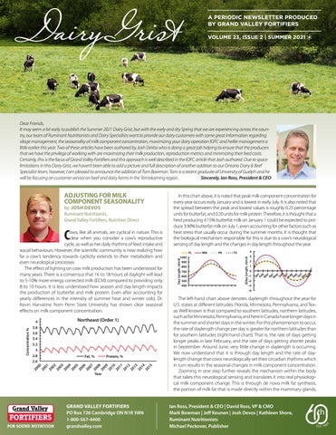
In this chart above, it is noted that peak milk component concentration for every year occurs early January and is lowest in early July. It is also noted that the spread between the peak and lowest values is roughly 0.25 percentage units for butterfat, and 0.20 units for milk protein. Therefore, it is thought that a herd producing 4.15% butterfat milk on January 1 could be expected to produce 3.90% butterfat milk on July 1, even accounting for other factors such as heat stress that usually occur during the summer months. It is thought that the biological mechanism responsible for this is due to a cow’s neurological sensing of day length and the changes in day length throughout the year. Day Length, min/d

ADJUSTING FOR MILK COMPONENT SEASONALITY

-2 -3 -4

The left-hand chart above denotes daylength throughout the year for U.S. states at different latitudes: Florida, Minnesota, Pennsylvania, and Texas. Well known is that compared to southern latitudes, northern latitudes, such as for Minnesota, Pennsylvania, and here in Canada have longer days in the summer and shorter days in the winter. For this phenomenon to occur, the rate of daylength change per day is greater for northern latitudes than for southern latitudes (right-hand chart). That is, the rate of days getting longer peaks in late February, and the rate of days getting shorter peaks in September. Around June, very little change in daylength is occurring. We now understand that it is through day length and the rate of daylength change that cows neurologically set their circadian rhythms which in turn results in the seasonal changes in milk component concentration. Zooming in one step further reveals the mechanism within the body that takes this neurological sensing and translates it into real physiological milk component change. This is through de novo milk fat synthesis, the portion of milk fat that is made directly within the mammary glands, Ian Ross, President & CEO | David Ross, VP & CMO Mark Bowman | Jeff Keunen | Josh Devos | Kathleen Shore, Ruminant Nutritionists Michael Peckover, Publisher

as opposed to simply derived from the diet or body fat reserves. The work by Dr. Harvatine has demonstrated that 50% of the variation in the seasonality of milk fat concentration is directly attributed to the ability of the mammary gland to manufacture this milk fat. This is how a cow flips the switch on and off for milk fat concentration as the seasons change. Now that we know this, what do we do with this information? The first step is to set benchmarks for your herd for different points throughout the year. Using DFO statements, milk testing, or robotic milk recording software, determine what your components through the year are on average. Taking these averages, add 0.125 or 0.10 points for milk fat and protein, respectively, and this should set a benchmark for around January 1st milk shipped. Conversely, subtract around 0.125 or 0.10 points for what the benchmark will be for around July 1st. These benchmarks will then be able to serve as a reference throughout the year for where your herd “should” be at, all other factors being held equal. With that said, how can we best maximize our return on investments while adjusting for seasonal milk component changes throughout the year? Strategies to achieve this include the feeding of highly digestible forage sources, such as BMR corn silage or some grass silages, as well as maintaining adequate physically effective fibre levels. Maintaining an appropriate level of rumen-available energy and protein is also important to ensure the rumen microbes can thrive and produce the substrates necessary for de novo fatty acid synthesis. In the early summer period, when the cow’s capacity to naturally produce milk fat through de novo fatty acid synthesis is lowest, the question may become “how can I best target my resources to overcome or adjust for this seasonal decline in milk fat concentration?”. First ask yourself if there is even a problem to begin with. For example, if the herd’s milk fat is 0.125 points lower than the yearly average, and there is no pressing need to push cows to fill more quota or incentive days, allowing the milk fat to naturally lower may be the most cost-efficient strategy while not causing any malfunctions in the rumen. If more milk fat is needed to fill quota or incentives and de novo fat is maximized through the feeding strategies above, then using research proven additives or adding/increasing palm fat in the diet may pay. Of course, seasonality is not the only factor that can decrease component concentrations during summer. Heat stress may decrease component concentrations lower than what can naturally be expected from seasonality. Managing heat stress well tends to pay back during a time when component yields are needed to fill quota and to maintain a producer’s cull rate. To do this, crucial management factors include adequate cooling from ventilation or sprinklers, feeding cows multiple times per day to maximize eating potential and therefore rumen health, as well as adding water to TMRs when needed to allow for reduced feed sorting. Nutritional additives or feedstuffs should also be evaluated. Strategies include swapping out highly fermentable energy sources for highly digestible non-forage fibre sources, feeding palm fat, and increasing the DCAD of the diet with sodium and potassium to account for the loss of these crucial minerals through sweat. Specific science-proven feed additives have also been shown to have a high return on investment to combat heat stress and optimize or adjust for seasonal decline in component yields. Additives suggested by Grand Valley Fortifiers include live yeast which has been shown to result in improved rumen health and fibre digestibility. Furthermore, research-based essential oil products have been shown to optimize energy extraction from the diet, improve meal frequency, and enhance water intake. The recent advances in the understanding of how seasonality affects the concentration of milk components should lead us to set benchmarks throughout the year. Within a given time period, evaluating when to search for lost component opportunities and when to adjust for naturally lower component concentrations will lead to increased profitability. If you have any questions, Nutrition Direct or your local GVF Specialist would be happy to help you evaluate your specific benchmarks and targeted management and feeding strategies for the best possible return on investment. ■

TIPS FOR ENSILING GREAT SILAGE

by: PAUL WIGHT, CCA-ONT Technical Service Manager, Robinson Bioproducts Inc.

y job with Robinson’s Bioproducts in Ontario has been to complete on farm bunk audits for our Chr. Hansen silage inoculant customers. After more than 1200 bunk audits I believe farmers that do a great job at filling their bunks have few if any issues at feed out with poor feed. As the saying goes “garbage in garbage out” or I prefer “quality silage in quality silage out.”

Dry Matter Losses can account for Loss of Feed It is important to realize dry matter losses are costly, Table 1 shows the dry matter losses from different storage systems. In bunker silos and drive over piles there is a direct relationship between dry matter losses and Table 1: Typical Ranges of DM Loss bunk density. See Table 2. Silo Type Range Keep in mind if you are looking for Oxygen-Limiting 4-8% more bunk space, you can increase silage bunk density from about 15 Stave Tower 6-12% lbs./cu ft to 17 lbs./cu ft and put more Bunker 12-30% silage in the same space just by doPile 12-30% ing a better job at packing. So, let us review the key points of Bag 4-40% putting up quality silage: Wrapped Bale 2-50%

Crop Moisture Table 2: Dry Matter Loss as Influenced by Silage Density (Ruppel, 1992)

DM Density DM Loss, (lbs DM/ft3) 180 Days (%) 10

20.2

16.8

15.9

15.1

Forage moisture plays a critical role in a successful ensiling process (Table 3). When forage moisture is too low, it is difficult to pack the ensiled material. As a result, air can remain trapped within the forage mass. This encourages yeast and mold growth, which leads to excessive heating and loss of DM.

Crop Maturity

Stage of maturity of the forage crop at harvest is an important fac22 10.0 tor in determining nutritional value. Maturity affects both silage yield and quality. Forage yield usually increases with advanced maturity, while nutritional value usually decreases. It is generally recommended to harvest whole-plant corn when the milk line is 2/3-3/4 of the way down the kernel. At this point, the moisture of the whole plant will normally be 64 to 68 percent. This makes packing easier and assures adequate fermentable sugars for the Lactic Acid Bacteria (LAB) and maximum energy value for livestock. Recommended maturity for alfalfa is the mid-bud to early bloom stage. A delay in harvesting decreases protein content and increases acid-detergent fiber and neutral detergent fiber values. 18

13.4

Weather Weather conditions at harvest are a major concern for alfalfa, but less of a concern for corn. Alfalfa contains 75 to 80 percent moisture at cutting and should always be wilted in the field before ensiling to prevent effluent and potential clostridial fermentation. The amount of time required to wilt alfalfa depends on the weather. Warm and windy conditions should dry the forage to about 65 percent moisture within four to six hours. If temperatures are cool or the humidity is high, the wilting period is prolonged.

Dairy Grist Table 3: Recommended moisture/stage of maturity of crops at the time of harvest/ensiling

Crop

Moisture (%)

Maturity

Upright Conventional

OxygenLimiting

Bunker Trench or Pile

Alfalfa

55-65

50-60

55-65

60-65

Mid-bud to early bloom

Alfalfa Grass Mixtures

55-65

50-60

60-65

Mid-bud to early bloom for alfalfa boot

Corn (Whole Plant)

62-68

50-60

64-68

Milk line 2/3 to 3/4 down the kernel*

Grasses (Perennial Cool Season)

55-65

50-60

64-70

69-65

Boot

Bermuda Grass (Small Grains)

64-68

55-65

64-68

14-18” in height, boot to dough

Bermuda Grass (Whole Plant Grain & Forage Sorghum)

64-68

50-60

64-68

Late milk to late dough in grain

Silo Bag

* Chop the material and test - milk line can sometimes be unreliable.

Chop Length Forage that is chopped at the recommended length promotes good packing, faster air exclusion, and even distribution in the silo. Forage that is chopped too coarse is difficult to pack and traps oxygen and can be easily sorted at the feed bunk. This can result in excessive heating from a prolonged aerobic phase and increased yeast and mold growth. For corn silage be sure that you are getting the kernels processed to the desired level that you and your Grand Valley Fortifers representative are wanting.

with JOSH DEVOS Ruminant Nutritionist, Grand Valley Fortifiers, Nutrition Direct

MAXIMIZING IOFC ON YOUR DAIRY OPERATION Income Over Feed Cost (IOFC) = Milk Income - Total Feed Costs This equation is one of many measures dairy producers consult when considering their operation’s profitability. IOFC is used when a producer wishes to evaluate the cost efficiency of their nutrition program. The strategy behind this measure is to maximize the milk income you receive and minimize the total feed costs you pay. This makes sense mathematically. However, how is IOFC maximized in the real world? Assessing the relationship between IOFC and various easily measured on-farm metrics yields interesting results demonstrated through plotting the relationships. The first is the relationship for IOFC and daily milk production as tracked by the GVF-Feed-Cost-Calculator Records for 267 Holstein dairy farms.

Silage Additives Of the various types of silage additives available, bacterial inoculants are the most widely used. A silage inoculant should contain live, acid bacteria and should provide at least 100,000 Colony Forming Units per gram (CFU/g) of wet forage. Farmers Farmacy, a division of the GVF group of companies carries Chr. Hansen silage inoculants. Their people are very experienced in helping you select the correct inoculant for your crop.

Applicators A uniform distribution of a bacterial silage inoculant on forage is important for maximum product effectiveness. Start the season by calibrating your applicator. Also keep in mind applicator temperatures; -you need to keep the water temperature cool. “Do not allow the temperature of the water in the applicator tanks to rise above about 100⁰F or 38⁰C as this may decrease the viability of the bacteria.” (Mulrooney and Kung 2008)

This graph above demonstrates that daily milk production explained nearly 79% of the variation in IOFC between these farms. There is strong linear relationship here that predicts that if milk production explained 100% of the variation in IOFC, then each additional litre of milk produced per cow per day will result in an additional 57 cents in IOFC. The key takeaway from this graph is that increasing milk production is the overwhelming driver of what determines the IOFC from farm to farm. In contrast to this clear relationship, the below graph demonstrates the relationship on those same farms between IOFC and daily purchased feed cost per cow.

Filling and Packing Perhaps more nutrients are lost when silo filling is prolonged than at any other time of silage management. Regardless of silo type, filling, packing, and sealing should be completed as quickly as possible to achieve anaerobic conditions necessary for optimum fermentation, storage, and feed out. During filling, always distribute forage evenly and in thin layers. In upright silos, use a distributor to avoid separating coarse and fine forage materials. In trench, bunker, or drive-over piles, use a heavy wheeled tractor which travels back and forth over each layer of forage. Completely cover and seal the silage surface with four-to-six-millimeter plastic and weigh down the entire surface of the plastic with discarded tires or tire walls. ■ Information Source; Chr. Hansen Insure High Quality Forage

This graph demonstrates that on those same farms, Purchased Feed Cost explained a negligible amount (3.4%) of variation in what determines IOFC from farm to farm. That means there are many producers with high IOFC and high purchased feed costs and farms with very low IOFC

grandvalley.com

and low purchased feed costs, and vice versa for both. Basically, there is no relationship between the IOFC and Purchased Feed Cost. Therefore, to maximize IOFC, focusing on increasing milk production per cow is much more important than focusing on decreasing purchased feed cost per cow. This is not to say that purchased feed costs are unimportant, as it is indeed mathematically embedded into the IOFC equation. However, first importance should be placed on milk production, and then secondary importance on purchased feed cost – specifically ensuring that the highest level of milk production is paired with the lowest possible level of purchased feed that is sustainable to achieve that highest level of milk production. To conclude, analyzing some of the basic farm to farm differences in IOFC yields the clear conclusion that focusing on maintaining a high level of milk production per cow is the most successful strategy to maximize IOFC. Wherever a producer is currently at on the spectrum of this key profitability indicator, a primary focus on milk production and a secondary focus on maximum returnon-investment nutritional solutions will result in steps in the right direction. Our Nutrition Direct team or your local GVF Dairy Specialist would be happy to help you determine specific solutions to maximize IOFC on your herd. ■

with BRIAN NELSON Dairy Specialist, Grand Valley Fortifiers

Q1: Is my heifer rearing strategy working? Widespread use of sexed semen creating a lower demand for replacement heifers (not to mention overfilling our barns with youngstock) has created a situation where fresh cow prices do not cover the full cost of raising these animals. Crowded facilities, low forage inventories, and rising land prices across the country are placing renewed focus on heifer rearing strategies. Most producers chronically underestimate the cost of raising replacement animals. From our work at GVF, we estimate heifer raising costs to be between $3000 – $3500 when true costs are evaluated. For producers raising a continuous surplus of replacement animals, the replacement costs of animals kept is much greater. For example, if a producer raises 10 animals to calving, the cost of raising these replacement animals is $30,000. If 5 are sold for $1500 each, this generates a “profit” of $7500. However, when you subtract this “profit” from the total heifer program costs, this loss is absorbed by the animals kept. Meaning, $30,000 minus $7500 divided over the 5 animals kept results in a rearing cost of $4500 per head for the animals kept. Another point to note is that daily costs of raising heifers is not the same for every day of life. Historically, approximate heifer raising costs have been $3 per head per day. We need to remember the cost per day is significantly greater during the milk feeding phase. The true cost of raising calves on milk can be as high as $10/ day for some operations. This means, any heifer rearing strategy needs to start nine months before the calf is born to make the biggest impact on your programs bottom line. The last thing to consider is how long it will take a heifer once she is a part of the milking herd to pay back to the farm. If culling happens too often in first or even second lactation, it is time to turn back to the calf/heifer raising program to see what bottlenecks might be occurring.

35% culling rate, 24 month age at first calving, and 4% non-complete rate on heifers will require 46 replacement heifers / year. Using these same values but changing culling rate to 45% will increase the annual number of replacement heifers by 13. In examples 3 and 4 you can see the impact of changing age at first calving, and non-complete rate effect inventory requirements. Number of Heifers Required to Maintain Herd Size

Ex 1 Ex 2

Ex 3 Ex 4

Herd Size (Milking and Dry)

125

Cull Rate (%)

Age at First Calving (Months)

Non-Completion Rate for Heifers (%)

# of Heifers Needed/Year

Total Heifer Inventory Required

117

106

Q3: What should my strategy be moving forward? There is no one size fits all approach to raising heifers. Cutting back on heifer numbers requires some inventory analysis and calculations using farm specific values. Any changes to heifer rearing program should begin with clear goals moving forward. Operations with limited land base or facilities, or higher costs of forage production will benefit most from running a more efficient heifer operation. Closed herds, herds with future expansion, future management changes (robots), or high genetic value animals may benefit from carrying a larger buffer of additional animals. Similar to the formula discussed above, there is also a formula to predict the number of heifers produced per year. This can be calculated using the formula: herd size x (12 ÷ calving interval) x (percent female calves) x (1 – calf mortality rate) x (24 ÷ age at first calving). In example 1 in the table below, average industry values are used. Examples 2 to 5 show how changing each of these values influences the number of heifers produced / year. Expected heifer numbers vary greatly in each of these scenarios. It is important to use your own numbers to complete this exercise. Expected # of Heifers Produced/Year

Ex 1 Ex 2 Ex 3

Ex 4 Ex 5

Herd Size (Milking and Dry)

125

Calving Interval (Months)

13.5

13.5 13.5

Female Calves (%) Calf Mortality Rate (%)

125

Age at First Calving (months)

# of Heifers Produced/Year

109

131

102

109

# of Heifers on Farm

There is no clear answer what the right number of replacement animals is for each individual operation. In general, most dairy operations carry a small to large excess inventory of animals. Careful thought and consideration to heifer rearing goals, and input from your genetics, nutrition, and financial advisor will surely improve your replacement programs bottom line. ■

Thought for the Day

“When I shut up the heavens so that there is no rain, or command locusts to devour the land or send a plague among my people, 14if my people, who are called by my name, will humble themselves and pray and seek my face and turn from their wicked ways, then I will hear from heaven, and I will forgive their sin and will heal their land.” – 2 Chronicles 7: 13&14 13

Q2: How many heifers do I actually need? The number of heifers required depends on several factors including, herd size, culling rates, age at first calving, and the non-completion (culling) rates for heifers. The recognized formula to calculate the number of heifers required per year is: herd size (milking + dry) x cull rate x (age at first calving ÷ 24) x (1 + non-complete rate for heifers). The following table outlines four different examples of how manipulating each of these variables impacts the annual heifer requirements. For example 1, a 100 cow herd with 25 dry cows,

As sickness and challenge continue to weigh heavy on our spirit, may we remember where we can turn, to find healing for our land.