Solution manual for Business Statistics in Practice Bowerman O’Connell Murphree 7th edition

Full download link at: https://testbankbell.com/product/solution-manual-forbusiness-statistics-in-practice-bowerman-oconnell-murphree-7th-edition/

CHAPTER 2 Descriptive Statistics: Tabular and Graphical Methods

2.1 Constructing either a frequency or a relative frequency distribution helps identify and quantify patterns in how often various categories occur L02-01

2.2 Relative frequency of any category is calculated by counting the number of occurrences of the category divided by the total number of observations. Percent frequency is calculated by multiplying relative frequency by 100.

2.3 Answers and examples will vary

for Discrete Variables: Sports League

Most popular league is NFL and least popular is MLS.

US MarketShare In 2005

US MarketShares In 2005

Daimler-Chrysler

2.10 Comparing the two pie charts they show that since 2005 Ford & GM, have lost market share, while Chrysler and Japanese models have increased market share.

L02-01

2.12 a. 32.29% b. 4.17% c. Explanations will vary

L02-02 b. A frequency histogram represents the frequency in a class using bars while in a frequency polygon the frequencies in consecutive classes are connected by a line. c. A frequency ogive represents a cumulative distribution while the frequency polygon is not a cumulative distribution Also, in a frequency polygon the lines connect the class midpoints while in a frequency ogive the lines connect the upper boundaries of the classes.

2.13 a. We construct a frequency distribution and a histogram for a data set so we can gain some insight into the shape, center, and spread of the data along with whether or not outliers exist.

L02-03

2.14 a. To find the frequency for a class you simply count how many of the observations are greater than or equal to the lower boundary and less than the upper boundary. b. Once you get the frequency for a class the relative frequency is obtained by dividing the class frequency by the total number of observations (data points) c. Percent frequency for a class is calculated by multiplying the relative frequency by 100.

L02-03 b. Two humps, left side may or may not look like right side. c. Long tail to the right d. Long tail to the left L02-03

2.15 a. One hump in the middle; left side looks like right side.

2.16 a. Since there are 28 points you should use 5 classes (from Table 2.5).

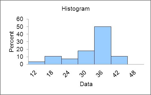
2.18 a. 6 classes because there are 60 data points (from Table 2.5) b. Class Length (CL) = (35 – 20) / 6 = 2 5 and we round up to 3. b. Shape of distribution is slightly skewed left Ratings have an upper limit but stretch out to the low side. b. Shape of distribution is slightly skewed right. Waiting time has a lower limit of 0 and stretches out to the high side where there are a few people who have to wait longer. c. The class length is 1 b. Shape of distribution is symmetric and bell shaped. c. Class length is 1

Distribution shape is skewed left L02-03 2.19a & b.

2.22 a. Concentrated between 3.5 and 5.5.

2.23 a. Concentrated between 48 and 53.

Distribution is skewed right and has a distinct outlier, The NY Yankees.

Distribution is skewed right

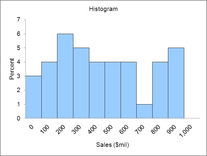
Distribution is relatively flat, perhaps two humped.

Distribution is skewed right. L02-03

2.26 The horizontal axis spans the range of measurements and the dots represent the measurements. L02-04

2.27 A dot plot with a 1000 points is not practical Use a histogram L02-03, L02-04

Distribution is concentrated between 0 and 2 and is skewed to the right. 10 and 8 are probably high outliers.

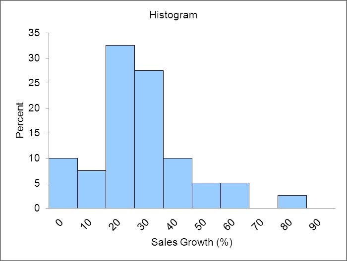
High outliers greater than 80%. Eliminating the high outliers the distribution is reasonably symmetric.

Low outliers 22 and 25. Without outliers distribution is reasonably symmetric.

L02-04

2.31 A stem & leaf enables one to see the shape of the distribution and still see all the measurements where in a histogram you cannot see the values of the individual measurements.

L02-03, L02-05

2.32 Displays all the individual measurements. --Puts data in numerical order Simple to construct

L02-05

2.33 With a large data set (eg 1000 measurements) it does not make sense to do a stem & leaf because it is impractical to write out 1000 leafs. Should use a histogram.

L02-03, L02-05

2.34 Stem Unit = 10, Leaf Unit = 1

L02-05

2.36 Rounding each measurement to the nearest hundred yields the following stem & leaf

Stem unit = 1000, Leaf Unit = 100 b. Bottle design ratings distribution is skewed to the left. a. Distribution is symmetric

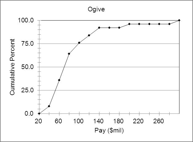
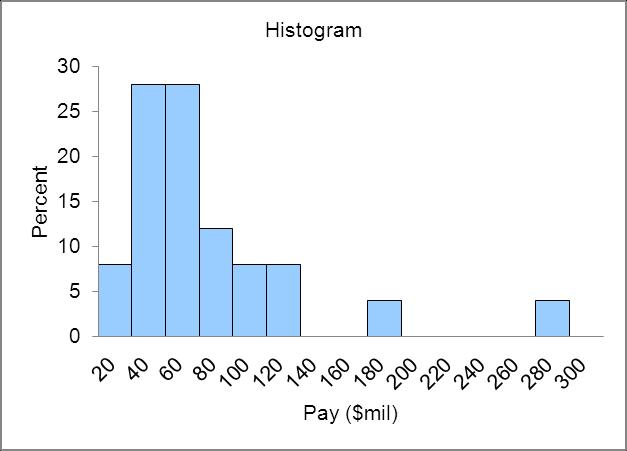
2.37 a. Payment times distribution is skewed to the right.

The 61 home runs hit by Maris would be considered an outlier, although an exceptional individual achievement b. Distribution of wait times is fairly symmetrical, may be slightly skewed to the right b. Distribution is slightly skewed to the left c. Since 19 of the ratings are below 42 it would not be accurate to say that almost all purchasers are very satisfied.

2.42 Cross tabulation tables are used to study association between categorical variables.

2.43 Each cell is filled with the number of observations that have the specific values of the categorical variables associated with that cell

2.44 Row percentages are calculated by dividing the cell frequency by the total frequency for that particular row. Column percentages are calculated by dividing the cell frequency by the total frequency for that particular column. Row percentages show the distribution of the column categorical variable for a given value of the row categorical variable. Column percentages show the distribution of the row categorical variable for a given value of the column categorical variable. L02-06 a. 17 b. 14 c. If you have purchased Rola previously you are more likely to prefer Rola. If you have not purchased Rola previously you are more likely to prefer Koka. a. 22 b. 4 c. People who drink more cola are more likely to prefer Rola. b. As income rises the percent of people seeing larger tips as appropriate also rises L02-01, L02-06

2.45 Crosstabulation Purchased?

2.51 a.

Appropriate Tip %BrokenOut ByThose WhoHave Left Without A Tip (Yes) and Those Who Haven't (No)

Appropriate Tip % b. People who have left at least once without leaving a tip are more likely to think a smaller tip is appropriate.

L02-01, L02-06

2.52 A scatterplot is used to look at the relationship between two quantitative variables L02-07

2.53 Data are scattered around a straight line with positive slope. L02-07

2.54 Data are scattered around a straight line with negative slope. L02-07

2.55 Data are scattered on the plot with the best line to draw through the data being horizontal. L02-07

2.56 Scatter plot: each value of y is plotted against its corresponding value of x. Runs plot: a graph of individual process measurements versus time L02-07

2.57 As home size increases, sales price increases in a linear fashion. A fairly strong relationship

2.58 As temperature increases, fuel consumption decreases in a linear fashion. A strong relationship.

L02-07

2.59 Cable rates decreased in the early 1990’s in an attempt to compete with the newly emerging satellite business. As the satellite business was increasing its rates from 1995 to 2005, cable was able to do the same.

L02-07

2.60 Clearly there is a positive linear relationship here. As a brand gets more sales, retailers want to give more shelf space. Also as shelf space increases sales will tend to increase. Its difficult to determine cause and effect here.

L02-07

2.61 The scatterplot shows that the average rating for taste is related to the average rating for preference in a positive linear fashion. This relationship is fairly strong.

The scatterplots below show that average convenience, familiarity, and price are all related in a linear fashion to average preference in a positive, positive, and negative fashion (respectively) These relationships are not as strong as the one between taste and preference.

L02-07

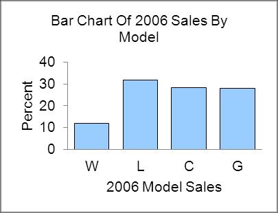
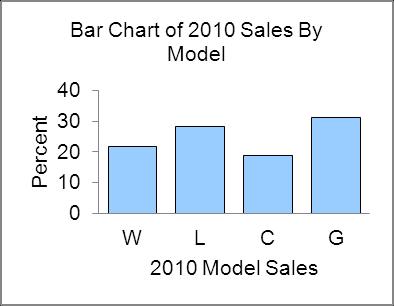
2.62 The differences in the heights of the bars are more pronounced.

L02-08

2.63 Examples and reports will vary.

L02-08

2.64 The administration’s plot indicates a steep increase over the four years while the union organizer’s plot shows a gradual increase.

L02-08 b. Yes, strong trend. c. The line graph is more appropriate because it shows growth. d. Probably not. Both distort the data.

2.65 a. No, very slight (if any).

L02-08

2.70 Written analysis will vary

2.71 Europe and the Pacific Rim both have a couple of outliers with ratings of 4 & 5, otherwise there does not seem to be much of a relationship.

Tabulated statistics: Area of Origin, Overall Quality Mechanical

2.72 Written reports will vary. See 2.69 for percentage bar charts. See 2.71 for row percentages.

L02-06

2.73 Pacific Rim has a much higher percentage rated 4 or higher than either Europe or United States.

Tabulated statistics: Area of Origin, Overall Quality

Design

2.74 Written reports will vary. See 2.70 for pie charts. See 2.73 for row percentages

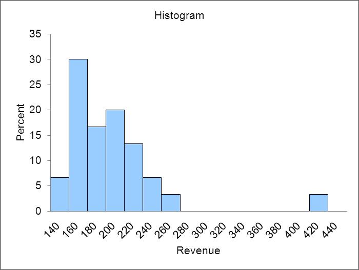
2.75 a. Since there are 50 data points you should use 6 classes. b.

Distribution is skewed to the right

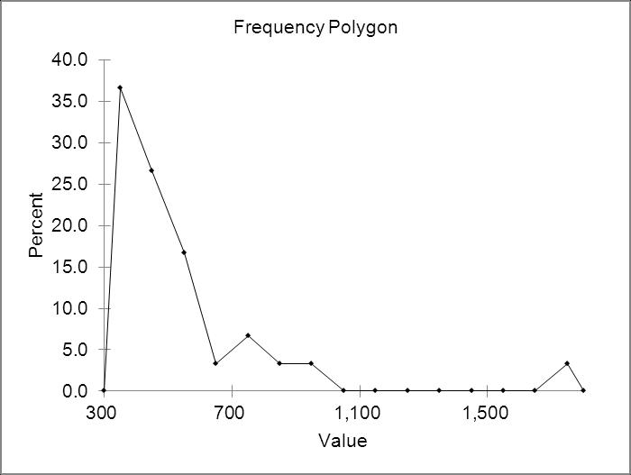
Distribution is skewed to the right

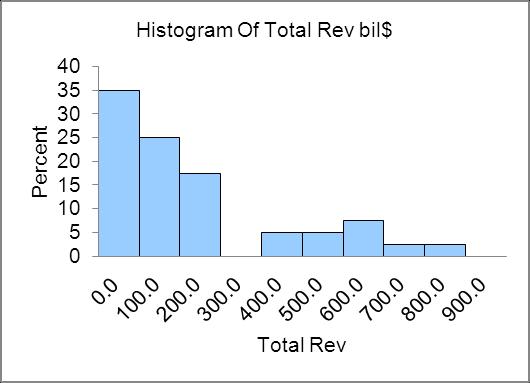
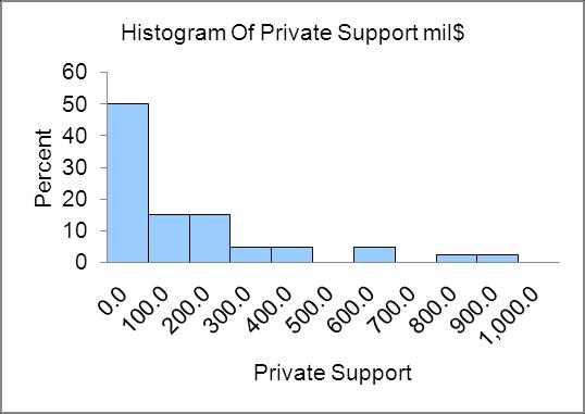
Distribution is skewed to the left

L02-03

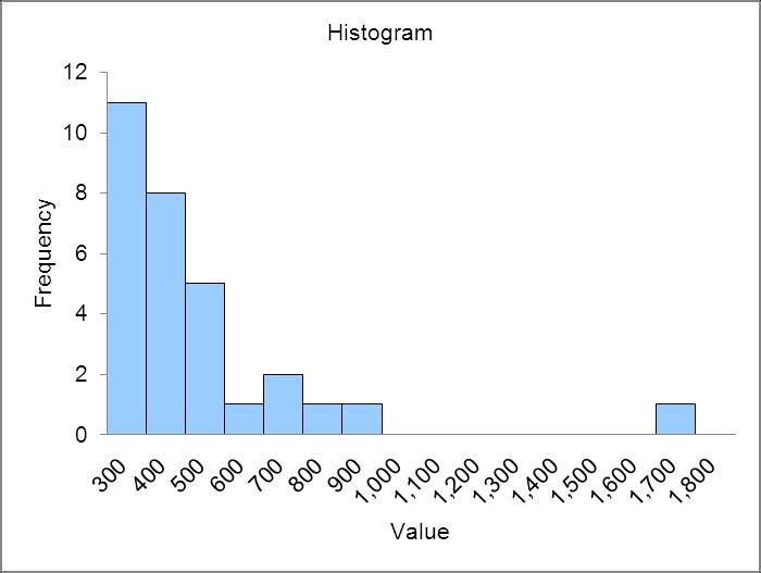
2.80 Distribution has one high outlier and with or without the outlier is skewed right.

L02-04

2.81 a. Class Factor Height

2.82 Since the runs plot is not in control, the stem & leaf is not representative of the number of missed shots.

2.83 The graph indicates that Chevy trucks far exceed Ford and Dodge in terms of resale value, but the y-axis scale is misleading.

L02-08

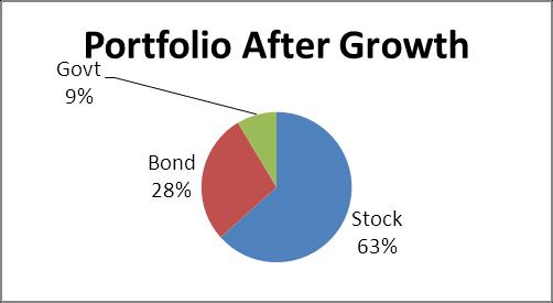
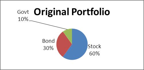
2.84 a. Stock funds: $60,000; bond funds: $30,000; govt. securities: $10,000 b. Stock funds: $78,000 (63.36%); bond funds: $34,500 (28.03%); govt. securities: $10,600 (8.61%) c. Stock funds: $73,860; bond funds: $36,930; govt. securities: $12,310