Issuu

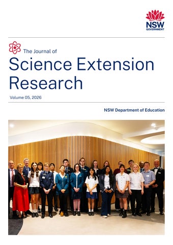
The Journal of

Science Extension Research Volume 05, 2026

NSW Department of Education

Contents

Quantifying crispiness Connor Reeves Galston High School

Foreword and introduction

Acknowledgement 8 Science Extension Showcase

Biological and medical sciences

Environmental and agricultural sciences

Physical and chemical sciences

Engineering and technology

Student reports

The Journal of Science Extension Research – Volume 5, 2026

Foreword The students represented in these pages have experienced something central to science: the need to think carefully, test ideas, revise assumptions and follow the evidence wherever it leads. For some reason, I can clearly recall having a number of different whale books opened at different pages, spread out on the floor of my bedroom on the farm. My window overlooked the back paddock where my pet cow was feeding on grass. It was seeing whales in books and watching the movie Free Willy as a child that ignited my passion forward to learn more and immerse myself in science. At the time I didn’t understand science or what the whales were doing in the books I read, I just knew I was interested and passionate about the world around me. Now as a whale scientist and mum, I look back and reflect on how I remember my childhood and very much saw science as a part of it. Secondary school is a time where students are learning not only about the world but also about themselves. It provides a platform for students to ask questions about the world and for many, carry out research for the first time. This is the time where students can delve a little deeper into topics of interest and be guided through the scientific process. They will soon discover that they may have just as many questions as they do answers and that scientific enquiry is a skill that one acquires that is useful throughout life. These skills have students think critically, think about how ecosystems work be it natural or human made. They start thinking bigger picture by scaling up ideas created in the classroom which may have real world impact. These skills then become part of our transferable skillset that we all carry with us beyond school and into professional fields. Allowing us to pivot when we want to.

The scientific process gives a structure or script on how science happens. It’s a process that enables others to replicate what we have done or understand what we have observed. Being part of science gives you the foundations to think critically and also with structure and purpose. It is about asking precise questions, designing methods, analysing evidence, dealing with uncertainty, communicating findings clearly, learning from setbacks. I remember when my masters on testing a whale alarm- a small device to alert whales of fishing gear presence- found that whales didn’t move away from the sound. I thought this was a failure but really, it was an important finding so I could share these findings with others who might be using similar technology. What is striking in this volume is how many students have looked closely at the world around them and found research questions hiding in plain sight. Their investigations reach into waterways, shorelines, reefs, soils, personal care products, medical materials, food textures and even imagined futures in space. In that sense, this journal reflects something I see often in my own work: science is not separate from everyday life. It is part of how we understand the places we live, the species we share them with, and the responsibilities we hold as custodians of land, water and sea. As a whale and wildlife scientist, I am especially drawn to the projects that connect young people with their blue backyard – studies of microplastics along shorelines and in bottled water, PFAS in the Snowy River, migratory birds in the Coffs Harbour region, crown-of-thorns starfish on the Great Barrier Reef, and changing temperate reef ecosystems in Eastern Tasmania. These investigations show students using science to ask questions that matter to communities, ecosystems and future decision-making. I also see the broader spirit of STEAM throughout this volume. Students are not only measuring and analysing; they are designing, modelling, communicating and imagining. Whether they are comparing EMG sensors for prosthetics, testing biodegradable plastic degradation, exploring biochar and soil health, asking whether bees could become space pollinators, or even quantifying crispiness, they are showing that science, technology, engineering, the arts and mathematics are deeply connected ways of making sense of the world.

The Journal of Science Extension Research – Volume 5, 2026

Dr Vanessa Pirotta Whale scientist/lecturer/author/woman in STEAM, Macquarie University

This is the kind of science communication we need: research that invites people in, connects evidence with lived experience, and helps communities, governments, industry and the public make better decisions together. If there is one thing I would like all of you to think about, it is this, you each play an important role in society. This is just the start of what might be an incredibly scientific journey. You need to think about what excites you and what you might be passionate about. It is OK not to have all the answers now. Your scientific journey has started. The path you travel on will be driven by passion, drive, determination and by surrounding yourself with people who help lift. There will be ups and downs- that’s normal. Say yes to opportunities and be kind to those who support the work you do. The future of science right here in Australia is more important than ever. We need bright minds and good team workers to collaboratively elevate Australia’s science sector. To support our growth in knowledge. This doesn’t mean making world first discoveries, it’s about the everyday you show up and add to the work you love. Together, that body of work may result in something wonderful.

Introduction Back in the eighties my parents made a wild investment, a set of Childcraft encyclopedias for four-year-old me. Throughout my childhood I repeatedly devoured volumes such as The Green Kingdom, The Animal Kingdom, World and Space and About Me, feeding my curiosity about the natural world and nurturing the budding scientist within.

It is somewhat embarrassing to admit how much I enjoyed completing projects in primary school, going deep on a topic, finding information from a range of sources then selecting the perfect colour of cardboard from the local newsagency to create a poster and proudly present my findings to the world. At high school, I was a highly interested and studious student who never found the learning material excessively demanding. However, once I started my science degree at university, I was overwhelmed by the leap in academic expectations and the dazzling intellect of my peers, and I felt completely out of my depth. This is one massive advantage for tackling the Science Extension course, it provides a safe stepping stone, a lofty leg up, or even a limitless launch pad for students on their path toward and beyond tertiary study. Students are guided in honing their skills to effectively question, research, reference, seek support, collaborate, problem solve, proofread, edit, and communicate, thereby setting them up for success as they move into the brave new world of university. For students embarking on the Science Extension journey, avoid being concerned if you do not possess the full range of skills as you begin, you will develop them along the way. Start early in choosing a topic that you are genuinely curious about. When you begin researching, you will find that the more you know, the more you realise there is to know, and if you keep going deep enough you will find a gap, that thing that isn’t known, and this is your money spot. Try to enjoy the journey, rather than being fixated on the end product. Don’t be afraid of setbacks, ‘no result’ may still provide an answer to your research question and any great scientist will agree that many great discoveries have resulted from a ‘failure’. The Science Extension course provides the perfect opportunity for students to step outside their comfort zone and push themselves to academic heights within a familiar and supportive environment. That said, it can be rather daunting to teach in a classroom with a small number of students, not having the answers, knowing less than the student about their topic and not wanting to hold them back or let them down. My advice to teachers is to try to be comfortable with the uncertainty and see it as a journey that you and you student are walking together, learning side by side. Along the way take every opportunity to inspire younger students in the hopes of creating a cultural shift towards the pursuit of excellence, perhaps engaging a junior The Journal of Science Extension Research – Volume 5, 2026

Felicity Abbey – Crookwell High School science class as ‘research assistants’ or having your students present their research proposals to Year 10 classes. Assist your students in connecting with the right mentors. After sending my student’s literature review and research proposal to academics working in the same field, I was overwhelmed and heart warmed by the level of assistance they were willing to offer through video conferences, emails, hands-on laboratory support and even checking in after course completion. You too will benefit from collaborating with others and I highly recommend making connections with other Science Extension teachers and the Science Curriculum Team through online meetings, emails and attendance at Masterclasses, to share in the spirit of generosity and learn through the experience of others. Share the progress of projects along the way by using your school’s communication channels to champion the creativity and courage of your students. The notion that a high school student can create new knowledge for the scientific community and the wider world is mind-blowingly exciting. Being part of my student’s journey, watching her project unfold was a privilege and one of the great pleasures of my career to date. Reading about the depth and quality of student work on such a creative, diverse range topics in the Journal of Science Extension Research fills me with confidence that the world is in safe hands when so many young people are courageous enough to systematically follow their curiosity. Enjoy reading the articles in this amazing volume and join me in being excited about what the future holds in the wonderful world of science. 7

Acknowledgement This edition includes research reports from Science Extension students who completed the course in 2025. All reports are the work of students studying in NSW public schools. They have been supported by their teachers and schools, and in some cases, external mentors. The Science 7-12 curriculum team acknowledges the incredible efforts of Science Extension teachers in inspiring, guiding and mentoring their students to complete their scientific research projects. Despite the novelty and innovatives of the syllabus, those teachers spared no effort to nurture their students’ scientific curiosity and engage them in conducting authentic scientific inquiry. As a result, their students have experienced new heights of academic and scientific achievements in their research journeys. To all NSW Department of Education schools, we thank you for your sustained efforts in achieving excellence in science education.

The Journal of Science Extension Research – Volume 5, 2026

We acknowledge the following teachers whose students’ reports appear in this publication: •

Felicity Abbey, Crookwell High School

•

April Barry, Ryde Secondary College

•

Bryce Blackmore, Kotara High School

•

Ian Bright, Marsden High School

•

Falguni Deb Chaudhuri, Turramurra High School

•

Andrew Dargan, Galston High School

•

Milena Driscoll, Barrenjoey High School

•

Blake Gruber, Mount View High School

•

Marina Gulline, Willoughby Girls High School

•

Gabriel Guy, Fort Street High School

•

Ben Harrison, Rose Bay Secondary College

•

Nicholas Holmes, Lake Macquarie High School

•

Ebony Larrea, Blacktown Girls High School

•

Shae Martin, Lake Munmorah High School

•

Brett Mckay, Kirrawee High School

•

Laiju Menon, Northmead Creative and Performing Arts High School

•

Anthony Murphy, Tempe High School

•

Kurt Nicholson, Lambton High School

•

Helen Shandil, Wyndham College

•

Michelle Tory, Coffs Harbour Senior College

•

Ethel Venayagam, The Ponds High School

•

Craig Wallace, Tuggerah Lakes Secondary College The Entrance Campus

•

Tobie White, Armidale Secondary College

•

Taara Wilson, Katoomba High School

•

Ben Zuiderwyk, Albion Park High School

The Journal of Science Extension Research – Volume 5, 2026

Science Extension Showcase

Celebrating outstanding students The Science Extension Showcase celebrates the curiosity, perseverance and scientific skill of NSW public school students who have undertaken authentic research projects as part of the Science Extension course. Our inaugural showcase event, held on 19 November 2025, brought together students, families, teachers, judges and education leaders to recognise months of independent inquiry, experimentation and scientific communication. The evening highlighted the purpose of Science Extension: taking science beyond the textbook and into real-world investigation. Students shared research posters and presentations that demonstrated not only deep scientific understanding, but also creativity, problem-solving and the capacity to communicate complex ideas clearly to an audience. Major award winners were selected by a judging panel through a detailed, criteria-based evaluation of student research papers and projects. Judges considered the significance of each project, the quality of the methodology, creativity and innovation, scientific understanding, and the effectiveness of presentation and communication. They noted the exceptionally high standard of entries, with many projects separated by very small margins. The 2025 major award winners were: •

Florence Dark, Crookwell High School – Effects of mechanical stress on the release of microplastics in bottled water

•

Shuyan Lin, Lambton High School – Exploring the life cycle of Tenebrio molitor on a polystyrene diet: The potential for mealworms to reduce the impact of plastics in the environment

•

Trang Nguyen, Northmead Creative and Performing Arts High School – The effect of omega-3 fatty acids on lipase-mediated breakdown of visceral fat in middle-aged women

•

Melody Rivard-Hyde, Fort Street High School – Exploring the relationship between molecular properties and error in LogP computation

•

Tahlia Rowan, Lake Macquarie High School – Recycling nylon waste for medical sutures

The Showcase also acknowledged the important role of teachers, mentors and judges in supporting young researchers. The projects demonstrated the value of explicit teaching of scientific writing, critical reflection and experimental design, while also showing what students can achieve when given the opportunity to pursue meaningful scientific question

Call for submissions For the opportunity to have your students’ research reports showcased in the next edition of the Science Extension journal, contact the Science 7-12 curriculum team. Email Science 7-12 curriculum team: Science7-12@det.nsw.edu.au

The Journal of Science Extension Research – Volume 5, 2026

Science Extension Showcase

The Journal of Science Extension Research – Volume 5, 2026

Biological and medical sciences

26 Colour as a diagnosis: Evaluating beetroot extract as a biosensor for pH and wound infection Lola Abrahams, Rose Bay Secondary College 33 Material discovery: Evaluating needle material sanitation efficiency beyond stainless steel Vieanna Agustin, Blacktown Girls High School 41 Effect of microplastics: Assessing the potential correlation between microplastic exposure and neurodegeneration or neurological issues within the human brain Lu-Anne Angwin, Katoomba High School 59 The effect of situational stress on heart rate and memory performance in secondary students: Cramming as a contributor to stress-induced cognitive impairment Bret Baltazar, Ryde Secondary College 66 Rhythms of readiness: The impact of music tempo on sports physiology and performance in application to warm ups Mira Bharathy, Northmead Creative and Performing Arts High School 79 Lung cancers caused by smoking and silica dust exposure: A comparative study of the genetic characteristics Reuben Carn, Galston High School 103 Antioxidant potential of herbal teas and their role in reducing age-related oxidative stress Purva Chaudhari, Northmead Creative and Performing Arts High School 112 The effect of allura red ac on cardiac activity using daphnia magna as an analogue Kodie Corpuz, Mount View High School

The Journal of Science Extension Research – Volume 5, 2026

120 How the culture of female health impacts quality of life, with a focus on endometriosis Annabel Dignam, Katoomba High School 132 The most common form of inner monologue experienced by individuals Ashley Dyer, Galston High School 142 Comparison of standing long jump and squat jump as predictors of maximal sprint speed in amateur male athletes Mitchell Gibson-Foad, Wyndham College 149 Associations between adolescent screentime and internalising and externalising symptoms: A correlational study Isabelle Keys, Albion Park High School 161 The illusory truth effect: Does repetition impact cognition? Jade Lin, Ryde Secondary College 170 The effects of chlorophyll content on photosynthesis efficiency Lily Michell, Turramurra High School 183 Comparing the antifungal activity of natural extracts and essential oils against aspergillus niger Lagan Nandha, The Ponds High School 191 The effect of omega-3 fatty acids on lipase-mediated breakdown of visceral fat in middle-aged women Trang Nguyen, Northmead Creative and Performing Arts High School 205 Investigating the antibacterial properties of turmeric extract Ananya Raut, Blacktown Girls High School

The Journal of Science Extension Research – Volume 5, 2026

217 Recycling nylon waste for medical sutures Tahlia Rowan, Lake Macquarie High School 224 Comparing antimicrobial properties of native australian essential oils against escherichia coli Angela Rowe, Willoughby Girls High School 233 Does the salt composition of Europa’s ice crust provide optimal abiotic conditions for life? Imogen Shaw, Kirrawee High School 252 Social desirability bias and the Hawthorne effect on adolescents’ self-reporting of screen time Jacob Stefas, Ryde Secondary College 266 Biomedical transfer method: Investigating the effect of polyethylene glycol molecular weight and concentration on gold nanoparticle aggregation in a high salt environment Abigail Watney, Kirrawee High School 278 The influence of odour-based mate-selection across taxa: Mice vs. humans Nina Wessen, Galston High School 284 Determining the effectiveness of sodium chloride in the inhibition of escherichia coli Chloe Winsley, Rose Bay Secondary College 291 Impact of alcohol consumption on total white blood cell count in smokers Hebe Ye, Ryde Secondary College

The Journal of Science Extension Research – Volume 5, 2026

Environmental and agricultural sciences

298 Investigating simple preventative measures against structured query language injection attacks Benjamin McCulloch, Albion Park High School 307 Comparative evaluation of emg sensors for constructing reliable prosthetics Riley Morgan, Lake Munmorah High School 316 Quantifying crispiness: An analysis into whether instrumental variables can be used to quantitatively measure crispiness Connor Reeves, Galston High School 325 Exploring the relationship between molecular properties and error in LogP computation Melody Rivard-Hyde, Fort Street High School 341 Proportion, paywalls and lag: Effect on global and australian scientific retractions between 1996-2022 Phalayna Tudhope-Betts, Coffs Harbour Senior College

The Journal of Science Extension Research – Volume 5, 2026

Physical and chemical sciences

350 Calculating the correlation between arthropod species maximum size growth and atmospheric oxygen levels Joaquin Adams, Rose Bay Secondary College 356 Microplastics in Australian personal care products: A persistent environmental concern Bonnie Andrews, Lambton High School 364 Impact of our shorelines on the fragmentation of microplastics Thea Barron, Lambton High School 374 Effects of age on the vulnerability of Tasmanian devils to DFTD Taketoshi Berry, Rose Bay Secondary College 382 Targeting nutrient transport in arbuscular mycorrhizal fungi: A sustainable approach to cereal yield enhancement Christian Burger, Fort Street High School 396 Modulating caffeine-induced metabolic stress: The protective role of L-theanine in saccharomyces cerevisiae viability Sanjana Chandramohan, The Ponds High School 408 Impact of pH on biodegradable plastic degradation Emelie Coe, Turramurra High School 418 Trends towards later autumn departure of East-Asian-Australasian migratory birds visiting the Coffs Harbour region Lani Cooper, Coffs Harbour Senior College

The Journal of Science Extension Research – Volume 5, 2026

432 Effects of mechanical stress on the release of microplastics in bottled water Florence Dark, Crookwell High School 448 Effect of acanthaster planci (crown-of-thorns starfish) on hard coral cover on the great barrier reef Katie Day, Armidale Secondary College 468 The effect of different strains of yeast has on the percentage of alcohol when brewing beer William Dorrian, Armidale Secondary College 476 The extent of lead contamination in Lake Macquarie and Cockle Creek David Farley, Lake Macquarie High School 483 Effects of biochar and gypsum application ratios on short-term nutrient retention in Australian soil Tia Forster, Kotara High School 492 Exploring the life cycle of tenebrio molitor on a polystyrene diet: The potential for mealworms to reduce the impact of plastics in the environment\ Shuyan Lin, Lambton High School 503 Investigation on the effectiveness of charcoal derived powdered activated carbon (pac) versus coconut derived granular activated carbon (gac) in adsorbing methanol from an aqueous solution of methanol, with and without ultraviolet regeneration Jasmine Lohanda, Marsden High School 510 Evaluation of m-cresol toxicity thresholds in brine shrimp (artemia sp.) Anton Ng, Rose Bay Secondary College

The Journal of Science Extension Research – Volume 5, 2026

520 Spatial heterogeneity of surface water PFAS levels along the snowy river, from its source to Lake Jindabyne Noah Riva, Barrenjoey High School 529 Mint oil extraction Ali Shahosseini, Marsden High School 542 Can bees adapt to hypogravity: Assessing the capability of bees as space pollinators Aarav Shrestha, Tempe High School 556 Exploring the effect of centrostephanus rodgersii range extensions on the biodiversity within temperate reef ecosystems of Eastern Tasmania Emily Sonter, Tuggerah Lakes Secondary College The Entrance Campus

The Journal of Science Extension Research – Volume 5, 2026

Engineering and technology

566 Beyond Habakkuk: Investigating pykrete in the 21st century Reuben Crispin, Lambton High School 576 Effect of UV-A exposure duration on physicochemical properties of distilled water Jazzieryl Pablo, Blacktown Girls High School 588 What are the optimal biomechanical factors to create the best human cannonball? Eehit Srivastava, Fort Street High School

The Journal of Science Extension Research – Volume 5, 2026

Colour as a diagnosis: Evaluating beetroot extract as a biosensor for pH and wound infection Lola Abrahams – Rose Bay Secondary College

Abstract This study investigated the use of beetroot extract as a natural indicator of pH changes, determining its ability as a biosensor for determination of wound infections. The dominant pigment in beetroots, betalin, undergoes significant colour changes in different pH environments. This investigation observes the interaction between beetroot extract to a range of bacterias to observe the colour change response. Results showed a change in all the extract samples, and a pH test was conducted on each bacteria after the beetroot extracts were removed, revealing a significant statistical difference between the bacteria groups ( F (2, 42) = F (27.849), p > 0.001 ). These findings suggest the potential for beetroot extract to become a tool in medical areas. However, this study is limited in its number of bacteria groups and slight gaps in the raw results. Implementation of beetroot extract as a sustainable medical tool would reduce medical waste production, rather contributing to green waste. It is an affordable and accessible tool, and can lead to the development of immediate wound infection detection which will accommodate medical industries and human health.

Literature review Wound Infections Wound infections occur when a substantial bacteria concentration is present in a wound, resulting in complications of impaired healing depending on the reaction of host defences and resistance to treatment including antibiotics (Anderson, 2009; Huang 2024). Wound infections can cause an increase of pain, epithelial bridging, hypergranulation, bleeding, a friable granulation bed, increased exudate, deterioration in the appearance of the wound and delayed healing (Physiopedia Contributors, 2024). Surgical site infections (SSI) are infections that develop as a result of an operation, and are synonymous with increased morbidity and mortality rates, longer hospital stays and significantly greater healthcare costs (SA Health, 2020). Early identification of infection is imperative to prevent it from spreading within the individuals’ body, or to others allowing for a reduction of greater risks (Ernstmeyer, 2021). Confounding variables that may increase the risk of infection in a wound include age, diabetes, hypertension, obesity, poor blood circulation, vascular disease and a weakened immune system (Faley, 2025). Untreated infections can possibly lead to serious health issues that may result in death, including systemic complications like bacteremia which often causes hematogeneous spread and sepsis. Cases of more severity can adopt organ failure or the exacerbation of existing comorbid conditions (Zabaglo, 2025). The clinical method to confirm if a wound is infected is through visual observations, which are confirmed through wound culture. Moreover, deeper infected wounds require more advanced technology to affirm an infected wound, including radiography, ultrasound imaging, thermography and more. Limitations of the current wound infection detection system include the expenses and scarcity of these technologies (Li, 2021). A need for highly specific, rapid and accurate methods is critical to determining infection in wounds, which should also be a simple process that does not require extensive training to ensure all infections are treated when first symptoms appear (Li, 2021).

Beetroot Beta Vulgaris (Beetroot) is a root vegetable distinguished by its red colour, and is rich in vitamins and minerals (Bjarnadottir, 2023). Beetroots contain a small portion of the pigments betalians, betacyanins and betaxanthins, however are predominantly composed of betanin by 75-95%, which is a water soluble red pigment found in the roots of beetroot. The colour of betanin is generally a constant dark red colour, however it will vary significantly due to pH exposure, where the colour will degrade significantly due to hydrolysis when in alkaline environments. As this investigation greatly focuses on the visual changes of beetroots, it is important to note that numerous confounding factors may influence the extent to which the colour changing occurs, including light, heat and oxygen (ScienceDirect, n.d.). Beetroots are generally a simple crop to grow,

The Journal of Science Extension Research – Volume 5, 2026

are notably resilient, and can be harvested in large quantities (RHS, n.d.). Their cost is highly dependent on seasons, however during optimum conditions for their growth, bulk buying beetroots is considered affordable (Torg, 2025). Moreover, plantation processes including soil preparation are not complicated to follow, making them an efficient and manageable crop to grow (Irvine, 2022).

Biosensors Biosensors are devices that generate signals of biological and chemical reactions, and it is appreciated as a tool in disease monitoring, drug discovery and detection of pollutants (Bhalla, 2016). Although making exponential progress over recent years, there are many limitations regarding their quality, including selectivity and poor performance, detection of cell viability, their response times and the complicated process of using them (Ali, 2022). However, due to their pigmentation, beetroots can serve as natural biosensors as a result of the fluorescence present in the pigment, generating a robust and reliable signal which can be easily detectable. A study conducted by Pratiwi 2025 concluded that betalain pigments are easily affected by pH, proving the halochromatic properties of the pigment in alkaline conditions. Pratiwi confirmed that a pH higher than 7 created a colour change on a spectrum from red to yellow-brown depending on the pH level (Pratiwi, 2025). This investigation proves the capability of beetroot to visually portray different pH conditions and can ultimately notify if there is an infection occurring within a wound.

Healthcare Resources Low to middle income countries experience significant healthcare resource challenges, resulting in poorer health outcomes and higher death rates than Western nations. Healthcare equity and improved overall health outcomes are essential for individuals living in these regions (NaturePortfolio, 2025). The global cultivation of beetroots makes it extremely accessible, and as a naturally grown resource it allows communities to create their own diagnostic tools without having to rely on international imports. The affordability of beetroot extract presents as a great innovation and alternative compared to synthetic biosensors which are often expensive and difficult to construct and use. Therefore, this study aims to investigate the use of beetroot extrat as a visual indicator for wound infections. It aims to determine whether beetroot extract will experience a change in colour when exposed to different pH environments.

Scientific research question Is there a change in beetroot colour when it is exposed to a bacteria with different levels of pH?

Scientific hypothesis Ha: Beetroot colour will change depending on the pH of Escherichia Coli (E. Coli), Staphylococcus epidermis (S. Albus), Bacillus subtilis (B. subtillis) H0: Beetroot colour will not change depending on the pH of Escherichia Coli (E. Coli), Staphylococcus epidermis (S. Albus), Bacillus subtilis (B. subtillis)

Methodology Preparing the Agar A sample size of 80 plastic petri dishes with powdered agar were prepared aseptically in an autoclave and left to solidify

Preparing the Beetroot Extract 2 beetroots were cut into small pieces and placed into a large measuring jug with 75mL of water. An stick blender was used to blend the beets, resulting in a liquid state with small lumps. This was poured through a sieve which was placed above a 200mL reagent bottle. The beet extract was pressed to drain substantial amounts of pure beet juice. Approximately 60mL was extracted through this process. Approximately 120 disks of filter paper were punched with a hole puncher, and placed in an empty petri dish, which was then soaked in the beetroot extract (Figure 1).

The Journal of Science Extension Research – Volume 5, 2026

Figure 1: Image of the filter paper disks soaking in the beetroot extract

Inoculation and Incubation The bacteria strains used in this study are E. Coli, K-12 strain, S. Albus and B. subtillis which were sourced from Southern Biological. 1mL of each bacteria was diluted in 49mL of water in a 50mL beaker. A micropipette set at 1mL was used to inoculate the bacteria in the agar. Each bacteria was inoculated in 20 different plates, and a control of 10 plates was also used. The plates were closed and sealed with tape to ensure no contamination or leakage occurred, then moved around to cover the entire agar with the bacteria solution. Each plate was placed in an incubator for approximately 24 hours set at 30℃. After incubation, 3 beetroot disks were placed in each petri dish and left for 24 hours.

pH Testing the Plates After approximately 24 hours the beetroot disks were removed. Small pieces of pH indicator paper were cut and placed inside the petri dishes to test the pH of each bacteria. After the indicator changed colour, it was compared to the universal pH indicator to determine the pH and recorded in a table for further data analysis.

Data Analysis Photographs were taken at some stages of the investigation to visually record the process and colour changes. Additionally, the pH of each plate was recorded in Excel where the mean, standard deviation and standard error were calculated. Those scores were then used to create a graph to compare the results of each bacteria, and a single-factor ANOVA was conducted for all the results, as well as a second ANOVA test without the Control group to compare the results with no constant. These tests produced F values and P values to determine the statistical significance of the groups.

The Journal of Science Extension Research – Volume 5, 2026

Results Prior Experiment Prior to this investigation a test was conducted to ensure that the beetroot extract would change colour due to different pH levels. This test soaked filter paper with beetroot extract in 6 solutions of different pH levels (1.4, 4.1, 5.5, 6.8, 8.6, 12.2), and confirmed that there would be a colour change in the beetroot when in different pH concentrations. It showed that in more alkaline conditions the beetroot extract became significantly lighter with yellow tones, whereas acidic conditions made the beetroot extract a darker purple colour (Figure 2). Figure 2: Image of the beetroot extract filter paper pieces after soaking in different pH concentrated solutions

Main Investigation After inoculating each petri dish containing the beetroot disks, there was an obvious significant colour change in the beetroot, suggesting the bacteria presented an alkaline environment. The disks in the Control plates did not have a distinct colour change, indicating the agar has a pH of 7. Figure 3: Graph showing the average pH of each bacteria after the placement of the beetroot disks (30 hours after)

The Journal of Science Extension Research – Volume 5, 2026

Table 1: Summary table of results B. subtilis had the highest average pH (9.93) and lowest variation (SD = 0.18, SE = 0.47), indicating both high and consistent results within that group. E. coli had a similar average (9.71) and a slightly greater variance (SD = 0.38, SE = 0.1). S. albus had a lower average (8.75) and a greater variance (SD = 0.68, SE = 0.17). The Control group was constant with an average of 7 and no variance at all (SD = 0, SE = 0). Overall, B. subtillis was the most reliable group due to its lowest variation score, whereas S. albus was the least reliable in both consistency and performance. The Control group serves as a baseline, being fixed at 7 with no variance (Table 1 and Table 2). A single factor ANOVA was performed to compare the effect of bacterial types on pH levels. The ANOVA revealed that there was a statistically significant difference of pH levels between the groups, F (2, 42) = F (27.849), p > 0.001.

Staphylococcus epidermis

Bacillus subtilis

Eschericia coli

Control

Average

8.75

9.933

9.714

Standard Deviation

0.683

0.176

0.378

Standard Error

0.171

0.469

0.101

Discussion Principle Findings This study aimed to determine the relationship between beetroot extract and different bacteria strains, wherein the results corroborate that once beetroot contacts the bacteria it will undergo a significant colour change. The average pH of each bacteria group confirms that they presented an alkaline environment, providing direct evidence of beetroot's capability to colour change in different pH conditions. Prior to this investigation, an initial experiment was conducted to ensure that beetroot would react to different pH conditions. By undergoing this procedure it was determined that alkaline solutions would create the most significant change in the original colour of the beetroot extract.

Study Limitations Measures were taken to ensure reliability in this investigation, including the repetition of experimental processes such as a variety of petri dishes used for each bacteria and multiple beetroot disks present in each plate. This ensures that all results are accurate and can provide an average for each data component. To guarantee validity in this study this included a control variable, each petri dish was firmly sealed, was not left exposed to air, and opened slightly when being innoculated to eliminate any potential air contamination. However, limitations in this study include the sensitivity of pH indicator paper, which only provides approximate values of pH. This reduces the accuracy of comparisons between different bacteria groups, mainly in regards to those with close averages. To ensure accurate results in future studies a pH meter would be the appropriate tool, which would provide numerical data rather than visual data. Moreover, although a sample size of 20 plates each were used, gaps in the data are present due to some plates becoming contaminated and therefore not included in the final results. This limits the reliability of the results and significantly impacts the mean of the datasets which further limits the accuracy when comparing the groups. Future studies must experiment with a larger sample size, increasing reliability and reducing the impact of possible data gaps. Additionally, only 1 strain of each bacteria was used in this investigation. Further research would need a variety of bacteria types and strains, as different strains used may yield different pH profiles, possibly significantly affecting the results of the investigation (Igẽno, 2018).

Possible Implications This study has direct implications in biomedicine and healthcare. This may be considered as a method of detecting infections present in wounds via surgical sutures or other potential methods that can safely be in proximity to a wound. Further, beetroots are a naturally grown product and wouldn’t participate in negative environmental impacts. They are an easy crop to grow and survive almost all soil conditions, indicating that production of beetroots for medicinal purposes would not prove impractical (Carnevale, 2009). Implementation of this method would greatly reduce wound infection related mortality rates, and would be an efficient and cheaper alternative to current technologies used to identify infection including biosensors. This process would

The Journal of Science Extension Research – Volume 5, 2026

assist in reducing the production of medicinal waste, which is currently 42 000 tonnes annually in Australia (Hitch, 2023). Further, a large majority of waste produced from this method would be green waste that can be reused for compost and other recyclable methods. Future research can investigate how differing pH levels affect bacteria growth and whether these changes could be used as visual indicators of bacteria types. A distinct colour change can correlate with a specific bacteria type causing an infection, allowing for rapid identification and efficient treatment of the infection.

Future Directions This investigation highlights the large demand for more reliable, accurate and valid research regarding the detection and monitoring of wounds with possible infections. The distinct change in colour of the beetroot extract when in contact with bacteria provides accurate results that this can be utilised in medicinal industries to detect infections. As discussed by Taylor, implementing the beetroot method of infection detection would effectively ‘remove financial barriers to medical treatment’, which is an extreme limitation of healthcare systems, which large percentages of the global population cannot afford (Huynh, 2021). This would ensure that future medical services would become accessible to a larger range of individuals, and be an equitable innovation in regards to the financial struggles commonly associated with healthcare. However, future research should test the impact of various bacteria and bacteria strains on beetroot extract to ensure that it has similar effects on a variety of infections. Future studies should compare this method with current methods used to detect infections, ensuring that it provides efficient results in order for doctors to react quickly and effectively once detecting a colour change in the beetroot extract. Further research into betalain pigments, including its pH properties and chemical behaviours, can assist in furthering this concept towards clinical applications. This method would reduce reliance on advanced equipment and can be vital in healthcare settings with limited resources. A combination of these future implications can establish a critical guide for determining infections in wounds to accommodate for the health of patients, whilst being a non-toxic and financially efficient method.

Conclusion This study has concluded that beetroot extract presents as a visual indicator of differing pH levels, offering significant colour changes ranging from a deep purple in acidic environments to a light yellow in alkaline environments. Prior to this investigation, minimal research has been done directly examining beetroot extract as a wound infection biosensor. This study presents preliminary evidence that beetroots can be developed into a simplistic yet highly effective diagnostic tool. Further research should involve a wider range of bacteria types and strains to ensure that a colour change will occur in a variety of bacteria types. In vivo experiments should be performed to deepen the understanding of beetroots’ colour changing properties on organisms, advancing towards implementing beetroot procedures in medical services to detect possible wound infections promptly. Further, extensive studies of betalin pigments as biosensors will provide an enhanced understanding of the potential of natural indicators. This method would contribute to a reduction of medicinal waste, instead producing substantial green waste, serving as a sustainable alternative for current technologies used for determining infection. This would lead to a significant decrease in wound-infection mortality rates, and would provide financial relief and support within healthcare systems whilst also being an accessible resource. This study is greatly relevant to the healthcare industry, and would ensure adequate treatment is possible to those with poor healthcare systems or a lack of advanced medicinal technology.

Reference list Ali, Q. (2022). Advances, limitations, and prospects of biosensing technology for detecting phytopathogenic bacteria. ScienceDirect. Anderson, S. (2009). Complications in Head and Neck Surgery. Wound Infection. https://www.sciencedirect.com/topics/pharmacology-toxicology-and-pharmaceutical-scie nce/woundinfection#recommended-publications Bhalla, N. (2016). Introduction to Biosensors. PubMed. https://pmc.ncbi.nlm.nih.gov/articles/PMC4986445/ Bjarnadottir, A. (2023). Beetroot 101: Nutrition Facts and Health Benefits. Healthline. https://www.healthline.com/nutrition/foods/beetroot Carnevale, T. (2009). The Veggie Patch. Gardening Australia. https://www.abc.net.au/gardening/how-to/thevegie-patch/9430378

The Journal of Science Extension Research – Volume 5, 2026

Ernstmeyer, K. (2021). Nursing Fundamentals. National Library of Medicine. https://www.ncbi.nlm.nih.gov/books/NBK591816/#:~:text=When%20an%20infection%2 0does%20occur,a%20major%20concern%20for%20nurses Faley, K. (2025). How to tell if a wound is healing or infected. OSF Healthcare. https://www.osfhealthcare.org/blog/how-to-tell-if-a-wound-is-healing-or-infected Hitch, J. (2023). How Does Medical Waste Affect The Environment? The Move Towards Eco-Friendly Medical Supplies. LFA. https://lfafirstresponse.com.au/blogs/how-does-medical-waste-affect-the-environment-the move-towards-eco-friendly-medical-supplies Huang, S. (2024). Point-of-care detection devices for wound care and monitoring. ScienceDirect. https://www.sciencedirect.com/science/article/abs/pii/S016777992300210X Huynh, A. (2021). A student harnessed the power of beets to make healing from surgery safer – and more equitable. CNN. https://edition.cnn.com/2021/04/17/us/student-beets-color-changing-sutures-wellness-trnd Igẽno, M. (2018). Study of pH Changes in Media during Bacterial Growth of Several Environmental Strains †. MDPI. https://www.mdpi.com/2504-3900/2/20/1297 Irvine, K. (2022). How to Grow Beetroot. Kath Irvine’s Edbible Backyard. https://www.ediblebackyard.co.nz/howto-grow-beetroot/ Li, S. (2021). Diagnostics for Wound Infections. National Library of Medicine. https://pmc.ncbi.nlm.nih.gov/articles/PMC8082727/#:~:text=Recent%20Advances:%20T raditionally%2C%20clinicians%20determine,in%20deeper%20wound%20infection%20d iagnosis Li, S. (2021). Diagnostics for Wound Infections. National Library of Medicine. https://pmc.ncbi.nlm.nih.gov/articles/PMC8082727/#:~:text=Conclusive%20and%20accu rate%20result%20for,%2C%20wound%20disruption%2C%20and%20bacteremia.&text= Obtain%20microbes%20below%20the%20surface,painful;%20may%20underestimate%2 0bacterial%20isolates.&text= NaturePortfolio. (2025). Medical devices for low-resource settings. NaturePortfolio. https://www.nature.com/collections/aahhffbcag/about-the-editors Physiopedia Contributors. (2024). Assessment of Wound Infection. Physiopedia. https://www.physiopedia.com/index.php?title=Assessment_of_Wound_Infection&oldid =362944 Pratiwi, R. (2025). Betalain Pigments: Isolation and Application as Reagents for Colorimetric Methods and Biosensors. MDPI. https://www.mdpi.com/2079-6374/15/6/349#:~:text=4.,17%2C19%2C20%5D RHS. (n.d.). How to Grow Beetroot. RHS. https://www.rhs.org.uk/vegetables/beetroot/grow-your-own SA Health. (2020). Surgical Site Infection (SSI) Surveillence. SA Health. https://www.sahealth.sa.gov.au/wps/wcm/connect/e1e50c80448142d39481965e88baaa69 /SSI_Surveillance+definition+-+FY+2022-2023+v1.1.pdf?MOD=AJPERES&CACHEID =ROOTWORKSPACEe1e50c80448142d39481965e88baaa69-oN4uawv ScienceDirect. (n.d.). Betanin. ScienceDirect. https://www.sciencedirect.com/topics/chemistry/betanin#:~:text=6.7%20Betanin,key%20 intermediate%20in%20all%20betalaines Torg. (2025). Beetroot Prices - Buy Beetroot in Bulk. Torg. https://usetorg.com/blog/beetroot-prices Zabaglo, M. (2025). Postoperative Wound Infections. National Library of medicine. https://www.ncbi.nlm.nih.gov/books/NBK560533/#:~:text=Complications%20arising%2 0from%20surgical%20wound,comorbid%20conditions%20may%20be%20exacerbated

The Journal of Science Extension Research – Volume 5, 2026

Material discovery: Evaluating needle material sanitation efficiency beyond stainless steel Vieanna Agustin – Blacktown Girls High School This investigation explored how needle surface material influences sanitation efficiency, measured by Escherichia Coli colony counts before and after autoclaving. The materials tested were titanium, silver, aluminium, and stainless steel, with the hypothesis that titanium would demonstrate the highest sanitation efficiency due to its resistance to inherent antimicrobial resistance. Thin-film coatings of each material were deposited onto glass slides, inoculated with E. Coli, and incubated before and after a single autoclave cycle. Colony counts were recorded for each condition and statistically analysed using paired T-Tests. The results showed that titanium, silver, and aluminium all achieved statistically significant reductions (p-value < 0.05) in E. Coli colonies post-autoclaving, while stainless steel did not. Silver exhibited the greatest microbial reduction overall, though titanium also performed strongly. These findings suggest that alternative materials may provide more effective and reliable sanitation outcomes than stainless steel, particularly in clinical or resource-limited settings. The data supports further investigation into the use of antimicrobial metals in hypodermic needle design to improve safety and reduce infection risk.

Literature review Hypodermic syringes are essential tools in diagnostic medicine, widely used for fluid aspiration and fine-needle biopsies during interventional procedures (Haseler et al., 2010). The effectiveness and safety of these procedures depend heavily on the quality and composition of the needle. Optimising needle materials is not only critical for enhancing patient comfort and reducing tissue trauma, but also for improving infection control Over the past century, stainless steel has become the industry standard for syringe needles due to its strength, corrosion resistance, and ease of fabrication. However, the healthcare industry’s increasing emphasis on safety, sustainability, and antimicrobial effectiveness has sparked renewed interest in alternative materials. Despite its mechanical benefits, stainless steel lacks inherent antimicrobial properties, making it prone to microbial colonisation and biofilm formation in the absence of rigorous sterilisation (Centers for Disease Control and Prevention [CDC], 2019). In low-resource clinical settings where sterilisation may be inconsistent, or in cases where needle reuse is unavoidable, this limitation poses significant risks. Stainless steel’s reliance on external sanitation methods, typically autoclaving, adds to workflow inefficiencies and leaves room for contamination. To improve surface performance, stainless steel needles are often coated with materials such as silicone or polytetrafluoroethylene (PTFE) to reduce friction and improve patient comfort. Studies have shown that these coatings can reduce insertion force and preserve needle sharpness (PMC, 2017; PDA Journal, 2022). However, these coatings do not offer antimicrobial protection and are neither biodegradable nor environmentally friendly. As Zhao et al. (2023) argue, there is growing pressure on the medical industry to shift towards more sustainable and biologically safe materials. Emerging research has identified metals like silver, titanium, and aluminium as promising candidates for needle construction due to their surface properties and potential antimicrobial activity. Silver, in particular, is renowned for its broad-spectrum antimicrobial effects. It operates through multiple mechanisms, including disrupting bacterial membranes, interfering with DNA replication, and impairing enzymatic functions (Rai et al., 2012). Titanium, widely used in orthopaedics, demonstrates excellent biocompatibility and mild antimicrobial action when oxidised. Aluminium, though less antimicrobial than silver or copper, is lightweight and can be surface-modified to enhance microbial resistance (Hosseini et al., 2021). Suzuki et al. (2020) evaluated the interaction between needle materials and tissue, finding that titanium and polymer-coated needles reduced insertion force and patient discomfort. Additionally, studies on costeffectiveness by Tran et al. (2024) showed that although materials like titanium have higher initial costs, their longer lifespan and lower infection risk yield long-term savings. Yet, those studies largely overlook sanitation efficiency, the extent to which these materials resist microbial contamination or are easily sterilised.

The Journal of Science Extension Research – Volume 5, 2026

Sanitation efficiency is a critical but underexplored aspect of material selection for medical instruments. Most studies focus on physical performance or user experience, while the comparative ability of materials to resist microbial growth post-sterilisation remains poorly documented. Autoclaving is the most common method of sterilisation, but it is energy-intensive, time-consuming, and not always accessible in low-resource contexts (World Health Organization [WHO], 2015). Materials that are intrinsically antimicrobial or easier to sanitise could dramatically improve safety and efficiency in clinical workflows. Recent research suggests that silver-coated surfaces retain antimicrobial activity even in the absence of chemical disinfection, offering potential advantages in high-risk or resource limited environments (Matsumara et al., 2019). Aluminium and titanium, while less potent, have also demonstrated resistance to microbial colonisation, especially when treated with surface-modifying technologies such as anodisation or thin-film deposition. These modifications enhance antimicrobial performance and can be scaled industrially for consistent application. Environmental sustainability is also a growing concern in medical device manufacturing. Stainless steel production is resource-intensive, requiring high energy inputs and generating considerable waste. In contrast, aluminium is highly recyclable, and silver or titanium may present lower environmental burdens when used as thin coatings (Zhao et al., 2023). The transition to single-use medical instruments has exacerbated medical waste, underscoring the need for materials that combine antimicrobial functionality with recyclability or biodegradability.

Scientific research question How does needle surface material affect the sanitation efficiency, measured by E. Coli colony counts, before and after autoclaving?

Scientific hypothesis Titanium-coated surfaces will demonstrate the greatest reduction in E. Coli colony counts after autoclaving, compared to silver, aluminium, and stainless steel, due to titanium’s biocompatibility and resistance to microbial colonisation.

Methodology This investigation was conducted as a first-hand experimental study with the methodology consisting of two key stages: (1) material selection and preparation, and (2) laboratory testing to assess sanitation efficiency. Material Selection: The selection of materials was informed by a literature review and collaborative discussions with the Research Facility Manager at the Research & Prototype Foundry (RPF), The University of Sydney. Three high-purity (5N, 99.999%) metals—aluminium, silver, and titanium—were selected for testing based on their known or potential antimicrobial properties and compatibility with thin-film deposition processes. Thin-film coatings of each metal were deposited using an AJA ATC-1800-E E-Beam/Thermal Evaporator (see Figure A1, A2 & A3) under high-vacuum conditions at the RPF. A consistent film thickness of 200nm was achieved across all samples, with each metal deposited onto 3 standard microscope glass slides per metal, serving as a uniform and inert substrate for controlled testing (see Figure A4). Surgical stainless-steel blades, sealed and unused, were included as the control group, representing the current industry standard for hypodermic needles. Gold and polymer-coated materials were considered but excluded from the study due to their high cost and incompatibility with the available deposition system. To ensure sterility and prevent contamination prior to testing, all prepared samples were handled with sterile forceps, placed in sterile Petri dishes, and stored under aseptic conditions. This preparation protocol enabled a focused and standardised comparison between conventional and alternative materials in terms of sanitation efficiency. Sanitation Efficiency Test: The sanitation efficiency of each material was evaluated through two sequential phases simulating typical sterilisation methods: 1.

Pre-Autoclaving Phase - standardised cleaning with ethanol.

2. Post-Autoclaving Phase - standard autoclave sterilisation. This dual-phase testing allowed for the assessment of how well each material resisted microbial contamination both before and after sterilisation procedures.

The Journal of Science Extension Research – Volume 5, 2026

Surgical stainless-steel blades, sealed and unused, were included as the control group, representing the current industry standard for hypodermic needles. Gold and polymer-coated materials were considered but excluded from the study due to their high cost and incompatibility with the available deposition system. Pre-Autoclaving Phase: Each material surface was inoculated with 100μL of a prepared E. Coli suspension, evenly distributed to simulate contamination. The samples were then left to dry in a sterile environment for 30 minutes to promote bacterial adhesion. Following contamination, a standardised cleaning procedure was performed using sterile gauze soaked in 70% ethanol, wiping each surface with three vertical and three horizontal strokes. The cleaned surfaces were allowed to air-dry completely under aseptic conditions. Each material was then swabbed using sterile cotton swabs moistened with 0.9% saline solution, applying a consistent zigzag motion to ensure coverage. The swabs were immediately streaked onto nutrient agar plates, which were incubated at 28℃ for 48 hours. Blank control plates were prepared using sterile, unused swabs to verify the absence of background contamination. Colony growth was visually assessed and recorded for each material. Post-Autoclaving Phase: After the pre-autoclaving test, the same set of materials was autoclaved at 121℃ for 15 minutes at 15 psi—a standard clinical sterilisation protocol. Once the autoclave cycle was completed and the samples cooled, they were retrieved using sterile forceps and handled under aseptic conditions. Each autoclaved surface was again swabbed using sterile saline-moistened swabs, which were streaked onto fresh nutrient agar plates. Blank control plates were also repeated. All plates were incubated under identical conditions (28℃ for 48 hours), and bacterial growth was again recorded.

Results Table 1 shows the average number of E. Coli colonies grown on each material before and after autoclaving. Titanium, silver, and aluminium surfaces all showed notable reductions in bacterial colonies following autoclaving, whereas stainless steel showed a smaller, non-significant decrease. Table 1: Average E. Coli colony counts (mean ± SD) before and after autoclaving, with corresponding p-values.

Material

Pre-Autoclave (mean ± SD)

Post-Autoclave (mean ± SD)

% Reduction

Stainless Steel

110.00 ± 10.00

80.00 ± 20.00

27.30%

0.1885

Titanium

93.33 ± 5.77

53.33 ± 5.77

42.90%

0.0202

Yes

Silver

220.00 ± 10.00

113.33 ± 5.77

48.50%

0.001

Yes

Aluminium

266.67 ± 4.71

136.67 ± 5.77

48.70%

0.0247

Yes

The Journal of Science Extension Research – Volume 5, 2026

P-Value

Significance (⍺ = 0.05)?

Figure 1. Average E. Coli colony counts for each material before and after autoclaving.

Figure 2 illustrates the percentage reduction in E. Coli colony counts for each material after autoclaving. Aluminium showed the highest reduction at 48.7%, closely followed by silver (48.5%) and titanium (42.9%). Stainless steel had the lowest reduction at 27.3%, reinforcing its comparatively lower sanitation efficiency. The trend clearly demonstrates that alternative materials outperform stainless steel in terms of microbial decontamination, with minimal variation between silver and aluminium. Titanium, although slightly less effective than silver and aluminium, still showed a notable advantage over stainless steel. Figure 2: Percentage reduction in E. Coli colony counts after autoclaving across the four needle surface materials.

The Journal of Science Extension Research – Volume 5, 2026

Discussion Results from multiple sources were obtained to perform analysis on the performance of bees in each of the three requirements. This investigation examined the sanitation efficiency of various needle surface materials by comparing E. Coli colony counts before and after autoclaving. The hypothesis proposed that titanium-coated surfaces would demonstrate the greatest reduction in bacterial contamination, based on its known biocompatibility and mild antimicrobial properties. Results from this experiment, however, revealed a more nuanced outcome, with silver and aluminium both demonstrating greater sanitation efficiency than titanium, although titanium still performed significantly better than stainless steel. Statistical analysis confirmed that titanium, silver, and aluminium all showed significant reductions in E. Coli colonies following autoclaving, while stainless steel did not. Titanium reduced colony counts by 42.9% (p = 0.0202), aluminium by 48.7% (p = 0.0247), and silver by 48.5% (p = 0.0010). Stainless steel, by contrast, only reduced colonies by 27.3% and did not show statistical significance (p = 0.1885). These findings challenge the assumption that stainless steel is optimal for needle sanitation and support the growing body of literature advocating for the exploration of alternative materials in clinical applications. Silver’s strong performance is consistent with extensive research documenting its potent antimicrobial effects. Rai et al. (2012) describes how silver ions disrupt bacterial cell membranes, interfere with DNA replication, and inactivate critical enzymes. These multi-targeted mechanisms explain the marked reduction in microbial colonies observed on silver-coated surfaces, even under short exposure conditions. Additionally, silver has been shown to inhibit biofilm formation, which is a major contributor to infection risk on reused or insufficiently sanitised medical tools. Although titanium did not achieve the highest reduction in colony counts, its sanitation efficiency was still statistically significant. Titanium is widely recognised for its biocompatibility and is often used in orthopaedic implants and dental tools due to its ability to resist bacterial adhesion when oxidised (Suzuki et al., 2020). The slight underperformance compared to silver may be due to titanium’s weaker intrinsic antimicrobial activity, but its consistent reduction in E. Coli colonies suggests that it remains a viable candidate for needle materials—especially in contexts where silver may be less appropriate due to cost or allergenicity. Aluminium’s strong performance was somewhat unexpected, as it is not typically known for antimicrobial activity. However, surface treatments such as anodization can significantly improve its microbial resistance (Hosseini et al., 2021). While this experiment did not include surface modification, the use of high-purity thin films may have contributed to more uniform and sanitisation-friendly surfaces, reducing microbial adhesion. Additionally, aluminium’s high thermal conductivity may facilitate more efficient heat transfer during autoclaving, contributing to improved sanitation outcomes. Stainless-steel’s relatively poor performance highlights a critical limitation in relying solely on sterilisation methods without considering material properties. Although widely used in medical devices due to its corrosion resistance and mechanical strength, stainless steel lacks antimicrobial action and is prone to microbial colonisation if not properly cleaned (CDC, 2019). Its lower reduction in E. Coli colonies compared to other materials supports findings from previous studies suggesting that sterilisation alone may not be sufficient to ensure infection control, especially in resource-limited settings or under repeated use conditions. These results provide valuable evidence that material choice can significantly influence the sanitation efficiency of hypodermic needles. They also suggest that sanitation protocols may need to be adapted based on the surface properties of the materials in use. While autoclaving remains the gold standard for sterilisation, its effectiveness is not solely dependent on temperature and pressure but also on how materials interact with microbial contaminants. The observed results support the argument made by Zhao et al. (2023), who advocate for integrating material science with infection control strategies to improve healthcare safety. Despite clear trends in the data, this study had several limitations. The sample size was small (n = 3 per material), which may limit the statistical power and generalisability of the findings. Larger datasets would improve the reliability of conclusions and help identify whether the observed differences are consistent across broader samples. Additionally, the materials were tested in the form of thin films on glass slides rather than real needle surfaces. Although this allowed for consistency and control in testing, the results may not fully reflect real-world mechanical, or surface conditions experienced during needle use. Another limitation lies in the use of a single microbial species. E. Coli is a suitable and well-understood test organism for contamination studies, but healthcare environments and clinical scenarios involve a diverse range of pathogens, including gram-positive bacteria, fungi, and viruses. Future studies should include a broader spectrum of microorganisms to better evaluate the antimicrobial scope of each material. Moreover, this study only examined the immediate effects of autoclaving. Longitudinal studies investigating repeated

The Journal of Science Extension Research – Volume 5, 2026

sterilisation cycles, biofilm formation over time, or long-term material degradation would provide a more comprehensive understanding of each material’s clinical suitability. Further research could also investigate how surface modifications—such as anodisation for titanium and aluminium or nanoparticle embedding in silver coatings—affect sanitation outcomes. Exploring the use of environmentally friendly coatings or biodegradable alternatives could also help align material development with growing demands for sustainable healthcare technologies. Environmental lifecycle assessments would be valuable in determining whether alternatives like aluminium and titanium present lower ecological burdens than stainless steel in long-term clinical use. Overall, this investigation highlights the importance of selecting materials that not only perform well mechanically but also support effective sterilisation and resist microbial contamination. The data demonstrates that titanium, silver, and aluminium each offer advantages over stainless steels in terms of sanitation efficiency. While the hypothesis predicted titanium would perform best, the findings suggest that silver was marginally more effective. However, titanium’s combination of biocompatibility, mechanical strength, and statistically significant antimicrobial reduction still supports its potential as a safer, clinically practical alternative. These insights could inform the next generation of hypodermic needle design and help reduce infection highs in both high-resource and low-resource healthcare settings.

Conclusion This investigation aimed to evaluate the sanitation efficiency of four needle surface materials—titanium, silver, aluminium, and stainless steel—by comparing E. Coli colony counts before and after autoclaving. The study was designed to address a gap in the literature concerning how different metals perform under sterilisation, focusing specifically on their ability to resist microbial contamination after a single autoclave cycle. The hypothesis predicted that titanium would demonstrate the greatest reduction in microbial growth due to its biocompatibility and known resistance to bacterial colonisation. While titanium did show a statistically significant reduction in E. Coli colonies (p = 0.0202), silver and aluminium both performed slightly better, with silver exhibiting the strongest statistical significance (p = 0.0010) and the highest overall reduction in microbial load Aluminium also showed a significant reduction (p = 0.0247), likely influenced by its thermal conductivity and surface characteristics, despite lacking strong inherent antimicrobial properties. In contrast, stainless steel, the current industry standard for hypodermic needles, exhibited only modest and statistically insignificant reduction (p = 0.1885) This suggests that alternative materials may offer improved sanitation efficiency and reduced infection risk, particularly in clinical environments where sterilisation resources may be inconsistent or compromised. While the results did not fully support the hypothesis, they provided meaningful insights into how material composition can influence sterilisation outcomes. Titanium remains a promising option due to its favourable clinical profile and performance, but silver’s potent antimicrobial activity warrants further investigation. Future research should expand the range of test organisms, assess long-term use and repeated sterilisation cycles, and explore surface modifications such as anodisation or nanoparticle embedding. These directions could inform the development of safer, more effective, and more sustainable medical devices that reduce infection risk and improve patient outcomes.

Reference list Benhamou, D., Weiss, M. C., Matthias Borms, Lucaci, J., Girgis, H., Cécile Frolet, Baisley, W. T., Gio Shoushi, Cribbs, K. A., & Wenk, M. (2023). Assessing the Clinical, Economic, and Health Resource Utilization Impacts of Prefilled Syringes Versus Conventional Medication Administration Methods: Results From a Systematic Literature Review. Annals of Pharmacotherapy. https://doi.org/10.1177/10600280231212890 Berardi, L. (2024). Comparison of the Cobalt Content in Needles Stainless Steel. PDA Journal of Pharmaceutical Science and Technology, 78(4), 520–521. https://doi.org/10.5731/pdajpst.2024.012977 Chan, E., Hubbard, A., Sane, S., & Maa, Y.-F. (2012). Syringe Siliconization Process Investigation and Optimization. PDA Journal of Pharmaceutical Science and Technology, 66(2), 136–150. https://doi.org/10.5731/pdajpst.2012.00856 Decontamination and Reprocessing of Medical Devices for Health-care Facilities. (n.d.). Retrieved July 5, 2025, from https://iris.who.int/bitstream/handle/10665/250232/9789241549851-eng.pdf

The Journal of Science Extension Research – Volume 5, 2026

Dhyani, A., Repetto, T., Bartikofsky, D., Mirabelli, C., Gao, Z., Snyder, S. A., Snyder, C., Mehta, G., Wobus, C. E., VanEpps, J. S., & Tuteja, A. (2022). Surfaces with instant and persistent antimicrobial efficacy against bacteria and SARS-CoV-2. Matter, 5(11), 4076–4091. https://doi.org/10.1016/j.matt.2022.08.018 Fernandes, R. M., Cary, M., Duarte, G., Jesus, G., Alarcão, J., Torre, C., Costa, S., Costa, J., & Carneiro, A. V. (2017). Effectiveness of needle and syringe Programmes in people who inject drugs – An overview of systematic reviews. BMC Public Health, 17(1), 1–15. https://doi.org/10.1186/s12889-017-4210-2 Fry Steel Company. (n.d.). 3 Benefits of Stainless Steel for Medical. Www.frysteel.com. Retrieved February 7, 2025, from https://www.frysteel.com/blog/3-benefits-of-stainless-steel-for-medical Haseler, L. J., Sibbitt, R. R., Sibbitt, W. L., Michael, A. A., Gasparovic, C. M., & Bankhurst, A. D. (2010). Syringe and Needle Size, Syringe Type, Vacuum Generation, and Needle Control in Aspiration Procedures. CardioVascular and Interventional Radiology, 34(3), 590–600. https://doi.org/10.1007/s00270-010-0011-z HMD Healthcare. (2023, June 14). Significance Of Stainless Steel Syringes & Medical Equipment in Healthcare. Hindustan Syringes & Medical Devices Ltd.; HMD. https://hmdhealthcare.com/blog/significance-of-stainlesssteel-syringes-medical-equipment-in-healthcare/ kdScientific Syringe Pumps & Dispensers. (2024). Stainless Steel Syringes - for high pressure and force, aggressive liquids (KDS). Kdscientific.com. https://www.kdscientific.com/kds-stainless-steel-syringes.html Naghavi, M., Vollset, S. E., Ikuta, K. S., Swetschinski, L. R., Gray, A. P., Wool, E. E., Robles Aguilar, G., Mestrovic, T., Smith, G., Han, C., Hsu, R. L., Chalek, J., Araki, D. T., Chung, E., Raggi, C., Gershberg Hayoon, A., Davis Weaver, N., Lindstedt, P. A., Smith, A. E., & Altay, U. (2024). Global Burden of Bacterial Antimicrobial Resistance 1990– 2021: a Systematic Analysis with Forecasts to 2050. The Lancet, 404(10459), 1199–1226. https://doi.org/10.1016/s0140-6736(24)01867-1 p1ws. (2025, January 6). Hypodermic Stainless Steel Tubing vs. Hypodermic Needles. Eagle Stainless. https://eagletube.com/about-us/news/hypodermic-stainless-steel-tubing-vs-hypodermic-needles/ Phlebotomy Training Specialists. (2022, September 12). The Bloody History of Medical Needles. Phlebotomy USA. https://www.phlebotomyusa.com/blog/history/the-history-of-medical-needles/ Rai, M. K., Deshmukh, S. D., Ingle, A. P., & Gade, A. K. (2012). Silver nanoparticles: the powerful nanoweapon against multidrug-resistant bacteria. Journal of Applied Microbiology, 112(5), 841–852. https://doi.org/10.1111/j.1365-2672.2012.05253.x Vo, A., Doumit, M., & Rockwell, G. (2016). The Biomechanics and Optimization of the Needle-Syringe System for Injecting Triamcinolone Acetonide into Keloids. Journal of Medical Engineering, 2016. https://doi.org/10.1155/2016/5162394 Wahab, M. A., Li, L., Li, H., & Abdala, A. (2021). Silver Nanoparticle-Based Nanocomposites for Combating Infectious Pathogens: Recent Advances and Future Prospects. Nanomaterials, 11(3), 581. https://doi.org/10.3390/nano11030581

Appendices Figure A1: AJA ATC-1800-E E-Beam/Thermal Evaporator

The Journal of Science Extension Research – Volume 5, 2026

Figure A2:. AJA ATC-1800-E E-Beam/Thermal Evaporator: INFICON SQC-310C Deposition Controller

Figure A3. AJA ATC-1800-E E-Beam/Thermal Evaporator: AJA International Phase II J Computer Control

Figure A4: Titanium after deposition onto microscope slides

Acknowledgements The expertise and direction of Mr. Nelson Briones, Facility & Program Manager, Research & Prototype Foundry, Core Research Facilities, University of Sydney, are gratefully acknowledged.

The Journal of Science Extension Research – Volume 5, 2026

Effect of microplastics: Assessing the potential correlation between microplastic exposure and neurodegeneration or neurological issues within the human brain Lu-Anne Angwin – Katoomba High School

Abstract This research project aimed to analyse the potential impact of microplastics and determine the possible correlation between microplastics and their effects on the brain or neurological functioning. Microplastics (MPs) can be classified as tiny plastic particles that range from 1nm to 5mm. They originate from plastic debris, ranging from large, manufactured products to cosmetics. These plastic products decompose over time to create microplastics. Due to their small size, they can be easily ingested and inhaled by humans and animals, along with the ability to pass through water filtration systems and enter major ecological ecosystems. The direct effect of microplastics on human health, particularly the brain, has not been investigated in past literature due to its relatively new nature. Therefore, the amount of data and articles that can be found is limited to the 20th century. This research focuses on a range of qualitative and quantitative aspects, including the measurement of microplastic concentrations ingested by humans and animals, as well as the effects that follow. Further research should be undertaken to determine the exact impact of microplastics on human health at high exposure levels, allowing for additional correlation.

Literature review Introduction Microplastics are increasingly recognised as a global contaminant of concern, with growing evidence of their presence across marine, freshwater, terrestrial and atmospheric environments. They arise from the fragmentation of larger plastics and the shedding of synthetic microfibers (Sun et al. 2022). Their small size raises concerns about potential human health impacts (Li et al. 2023). Recent research in toxicology and epidemiology has begun to link microplastic exposure with toxic effects on human health, specifically neurotoxicity (Zhang et al. 2022). Although research in this field is limited, the first notice of microplastics was in the late 1960s when small plastic pieces were discovered in the stomachs of albatrosses (Laysan Albatrosses Swallow Indigestible Matter on JSTOR 1969). However, the earliest mentions of microplastics in a human health-related context appear around the mid-2000s.

Microplastics Microplastics are primarily generated from the breakdown of larger plastic items through weathering, ultraviolet (UV) exposure and mechanical abrasion (Sun et al. 2022). Synthetic textiles also contribute substantially to the release of microfibres, which wastewater treatments cannot completely capture (Acharya et al. 2021). MPs are classified as plastic particles ranging from 1mm to 5mm (National Oceanic and Atmospheric Administration 2024). Human exposure to MPs occurs primarily through ingestion and inhalation, with estimates suggesting that individuals may consume up to 5 grams per week, roughly the weight of a credit card (Senathirajah & Palanisami. 2019). Additionally, recent research suggests that the human brain may contain as much as a teaspoon (7 grams) of microplastics (Nihart et al. 2025). This highlights the widespread presence of microplastics across food, water and air, raising concerns about potential effects on human health and neurological impacts.

Blood-Brain Barrier The brain is the most complex organ in the human body, acting as the control centre for the nervous system, which coordinates thoughts, memory, emotion, movement and vital bodily functions (Cleveland Clinic 2022). Weighing around 1.5 kilograms and roughly the size of two clenched fists, it is composed of 100 billion neurons The Journal of Science Extension Research – Volume 5, 2026

and a trillion supporting cells, used to stabilise the tissue of the brain. (Institute for Quality and Efficiency in Health Care 2016). The brain is shielded by the Blood-Brain Barrier (BBB), which prevents most toxins from entering neural tissue by restricting the circulation of toxins and pathogens that can cause brain infections. (The University of Queensland 2017). The barrier was first discovered in the late 19th century by physician Paul Ehrlich (Dyrna et al. 2013). It was later found that endothelial cells line the interior of blood vessels and are closely packed together, forming tight junctions (Dotiwala, McCausland & Samra 2019). Allowing only specific small molecules and some gases to pass freely through capillaries into brain tissue (The University of Queensland 2017). Larger molecules, such as glucose, gain entry through transporter proteins. Other components of the BBB also communicate with the barrier cells to change how selective the blood barrier is. (The University of Queensland 2017). However, the BBB can be compromised by systemic inflammation, originating in the gut (Arneth 2018). Neuroinflammation can occur from toxins or other unwelcome pathogens infiltrating the brain directly or indirectly through inflammatory pathways activated by gut dysbiosis (bacteria in the gastrointestinal tract) and the gut-brain axis (A two-way biochemical signalling between the Gastrointestinal tract and the central nervous system) (Sun, Koyama & Shimada 2022). Both routes highlight the potential for microplastics to trigger brain dysfunction due to microplastics' ability to cross the BBB. (Kopatz et al. 2023). Figure 1: Biological barriers that protect the brain. a) Blood–brain barrier, b) blood–CSF barrier, c) the arachnoid barrier (Kadry, Noorani & Cucullo 2020)

The Journal of Science Extension Research – Volume 5, 2026

Figure 2: Scale illustration of the BBB structure. Showing the tight junctions and structure of the BBB, the Left zoomed-in insert shows a disrupted BBB, allowing for transport of larger molecules through endothelial slits and pores, highlighting how MPs can cross the BBB if disrupted, as they are the same size as molecules within the BBB, scaled in nanometers (Belykh et al. 2020).

Immune responses in the brain The immune system plays a crucial role in protecting the body from pathogens and other forms of damage, ensuring host survival in an inhospitable environment (Mapunda et al., 2022). The brain's immune response is primarily mediated by microglia, which serve as brain macrophages in maintaining neuronal networks, regulating brain development, and facilitating injury repair, while also modulating neuroinflammation. Their uniqueness comes from their homeostatic phenotype and tight regulation of the central nervous system (CNS) microenvironment, making microglia different from other tissue macrophages (Colonna & Butovsky. 2017). Additionally, alterations in microglial functionality can be involved in brain development, aging, and neurodegeneration. Astrocytes are also involved in the neuroimmune system. Astrocytes are glial cells found around the brain. They form the BBB and the immune responses of the brain. They can release cytokines and other signalling

The Journal of Science Extension Research – Volume 5, 2026

molecules to maintain stable neural activity (Astrocyte - an overview | ScienceDirect Topics n.d.). Unlike astrocytes, which are embedded in tissues and are generally stable when resting, microglia remain in constant motion even in homeostatic conditions. When they are depleted, the microglia can migrate to repopulate areas within the CNS (Vainchtein & Molofsky. 2020).

Links to Neurodegeneration Dysregulated Immune responses in the brain are recognised as a driving factor of neurodegenerative diseases. When microglia become activated, they produce pro-inflammatory cytokines, which can lead to chronic neuroinflammation (Hansen, Hanson, & Sheng. 2017). This proinflammatory state can cause microglia to release cytokines that damage nearby neurons (Miao et al. 2023). Inflammation in the brain has been revealed to worsen neurodegeneration and contribute to the progression of Alzheimer’s disease (Leng & Edison 2020). Recent studies suggest that microplastics may intensify similar inflammatory pathways. Evidence showing that microplastics can weaken and/or cross the BBB, where microglia and astrocytes are activated to a proinflammatory state (Shan et al. 2022). These heightened levels of neuroinflammation may effectively prime the brain for earlier or more severe progression of disorders like Alzheimer’s and Parkinson’s, along with reduced cognitive functioning. Therefore, suggesting that the neurotoxicity of MPs may exacerbate or trigger neurodegenerative diseases and neurodevelopmental disorders (Asmaa et al. 2025).

Limitations and gaps Research on microplastics and their correlation with the brain is limited, affecting the full understanding of the effects of microplastics. Most studies rely on animal models or cellular structures, while evidence in humans is limited, with little data on long-term health outcomes. Additionally, the dose-response relationship is also unclear regarding the amount of exposure required to cause blood-brain barrier disruption, inflammation, or neurodegeneration. However, microplastics have been identified throughout the body. These gaps underscore the urgent need for environmentally realistic models and human studies to clarify the neurological risks associated with microplastic exposure.

Scientific research question Is there a correlation between microplastic exposure and neurodegeneration or neurological issues in the human brain?

Scientific hypothesis Null Hypothesis The resources analysed will indicate that ingested microplastics will have no significant effect on brain function, neurological health or associated pathways in humans and animals. Therefore, no link can be made.

Hypothesis If microplastics can cross the blood-brain barrier and trigger an immune response in the brain, then the existing literature will show a correlation between microplastic exposure and its contribution to neuroinflammation because they may accelerate pathways to neurodegeneration.

Methodology This investigation employs secondary data sourced from peer-reviewed journals and publicly accessible articles. The methodology was systematically designed to ensure reproducibility. Using electronic databases like PubMed, ScienceDirect and Google Scholar. These databases provided biomedical, neurological and interdisciplinary scientific research papers ensuring reliable and valid findings. Research was limited to peerreviewed publications from 2020 to 2025, as this is an under-researched and emerging field. Key search terms included multiple combinations of “microplastics and brain”, “microplastics and neurological effects”, and “microplastics and cognitive disruption,” to optimise retrieval of relevant studies. The studies found were then screened by title and abstract to remove irrelevant studies, ensuring that a comprehensive collection of relevant sources was obtained before applying inclusion and exclusion criteria. I created the predefined inclusion and exclusion data to ensure that appropriate data and articles found answered the research aim and question.

The Journal of Science Extension Research – Volume 5, 2026

Studies were included if they: -

reported qualitative findings on the effects of microplastic exposure on the brain, including cognitive function, neurological health, impacts and imaging evidence of microplastics in the brain.

Utilised human, animal or in-vivo methods that produced relevant insight into brain and microplastic impacts.

Were available online and published in the English language.

Studies were excluded if they: -

Focused exclusively on ecological or environmental impacts without neurological or brain impacts.

Were review articles (non-peer reviewed), commentary papers, editorials without original experimental observational data

Did not provide any measurable outcomes relating to brain function or cognitive function

Data extraction and analysis Data was extracted from the chosen studies for relevant information, including study design, sample type, exposure duration, type of microplastic and neurological outcomes. The data was then organised into tables, allowing for comparison across studies to identify recurring patterns and the impact of MPs.

Results Figure 3: Pie graph showing the distribution of research sources relating to microplastics and their effect on the brain (created in canva.com)

Figure 4: Key findings of studies linked to microplastics and brain health across cognitive, clinical and exposure research areas

Area of focus Reduced cognitive function (humans)

Key Findings -

Analysis of the human brains of decedents (deceased) revealed MPs and nanoplastics accumulate, especially in individuals with dementia.

MP levels in brain tissue were higher than in other organs. They increased dramatically from 2016 to 2024, with polymers polyethylene (PE) and polypropylene (PP) in high abundance throughout different organs.

The Journal of Science Extension Research – Volume 5, 2026

Reduced cognitive function (Animals)

Detected microplastics within the olfactory bulb, showing a direct pathway for MPs to enter the brain

Young and old female mice were exposed to MPs in drinking water over 3 weeks at different doses: • 0.0 mg/l (control) , 0.0025 mg/l (low dose), 0.025 mg/l (medium dose) and 0.125 mg/l (high dose) • Behavioural changes were observed; however, effects were more profound within older mice.

Dementia and Alzheimers

Effect through different levels of exposure and Ingestion

MPs were detected across all examined tissues, including brain, liver, kidney, heart, lungs and GI tract.

PS-MPs reduced Glial fibrillary acidic protein (GFAP) expression in brains from young and old mice

Polystyrene can penetrate the blood-brain barrier of mice

Exposure to MPs caused oxidative stress, inflammation and anxiety-like behaviour within mice (precursors to reduced cognitive performance)

MP in blood vessels can induce cerebral thrombosis (blockages in vessels). This can lead to neurobehavioral abnormalities

MPs are found in human cerebrospinal fluid (CSF) in people with Alzheimer's. Four types of microplastics found are polyethylene (PE), polypropylene, polystyrene and polyvinyl chloride (PVC).

Elevated PE and PVC levels correlated with lower CSF levels and a worse mini-mental state examination. Higher PE is related to a faster cognitive decline over a year.

Focus on microglial activation and neuroinflammation in Alzheimer's affected brains, providing support to MPs' exacerbation of dementia and alzheimers progression

estimation of exposure levels on humans per week,

Textile-based microfibres are defined as a primary exposure source

Experiments on mice were conducted using different dosages and exposure levels.

Figure 5: Illustration of the three mechanisms for microplastics to cross the blood-brain barrier. A) transcellular route, B) paracellular route and C) infected phagocyte route. (Evans 2020)

The Journal of Science Extension Research – Volume 5, 2026

Figure 6: Proposed pathway linking microplastic ingestion to neurological outcomes. Bottled water serves as a mode of transport for Microplastics, which can migrate into the cerebrospinal fluid. Once in the brain, microplastics contribute to the accumulation of amyloid-beta peptides, triggering neuroinflammation and subsequent neurodegeneration (He et al. 2025).

Figure 7: Table 1) Categorised 15 decedents highlighting their demographic and autopsy findings. All cases except 3 show no cerebral histological abnormalities. Table 2) 8 of the 15 decedents were identified with a total of 16 synthetic polymer particles and fibres, ranging from 1 to 4 microplastics per olfactory bulb (OB) (Luís Fernando Amato-Lourenço et al. 2024).

The Journal of Science Extension Research – Volume 5, 2026

Figure 8: a,b) Images of plastic particles within the brain using polarisation wave microscopy, visual fields were 15.4 and 20.1 μm wide, used to scan a section of the brain. Microplastics can 16 Student ID: 38732293 16 scatter light in distinctive waves or patterns, helping scientists distinguish them from normal biological tissue. c) White arrows highlight additional polarisation waves. d) flake-like or salad particulates following plastic dispersion with larger dimensions (<200 nm in length and < 40 nm in width). e, f) reveals more refractive inclusions (plastic particles) in dementia cases in regions associated with immune cell accumulation and (e) along vascular walls (Nihart et al. 2025).

The Journal of Science Extension Research – Volume 5, 2026

Figure 9: Overview of MP concentrations in the liver, brain, and kidney of all deceased samples. a) Microplastic concentrations in the liver, kidney, and brain of human samples, shown on a log10 scale, with the bar representing the group median value. Organ symbols in 2016 brain 17 Student ID: 38732293 17 samples were analysed independently at Oklahoma State University. b) Overall distribution of 12 different polymers, with polyethylene (PE) showing greater accumulation in the brain compared to the liver or kidney. c) PE (the most abundant consistently) concentrations in all organs display similar trends. d) Additional brain samples from specimens collected between 1997 and 2013 reveal that brain samples from decedents with diagnosed dementia (n=12, purple circles) exhibit higher MP concentrations than those without dementia. Additional Decedent samples sourced from Duke Kathleen Price Bryan Brain Bank in North Carolina (n=13, blue diamonds; NC), Harvard Brain Tissue Resource centre in Massachusetts (n=9, green diamonds; MA), National Institute of Child Health and Human Development Brain and Tissue Bank at the University of Maryland (n=5, orange diamonds; MD), and samples from New Mexico (red outline diamonds; NM). (Nihart et al. 2025).

The Journal of Science Extension Research – Volume 5, 2026

Figure 10: Alzheimer's disease effects on the blood-brain barrier: increased permeability, amyloid-beta buildup, inflammation, tau aggregation (protein involved in Alzheimer’s) (López-Ornelas et al. 2022)

Figure 11: A) visual illustration of the in vivo study design for 3 weeks of exposure to MPS in young and old female mice. B) concentration graph showing different doses (low, medium, high) measures for 10 hrs hourly without resuspension and at 24 hours with no resuspension (Gaspar et al. 2023)

The Journal of Science Extension Research – Volume 5, 2026

Figure 12: Micoplastics (PS-MPS) reduced the GFAP expression in the brains of both young and old female mice. A) Images of GFAP (Green) showed decreased expression throughout the whole brain, including the prefrontal cortex (PFC) and hippocampus (HIPPO). B) Decreased GFAP expression confirmed by Western blot. C) Quantification of decreased GFAP expression confirmed by t-test * p < 0.05. Scale bar = 1500 μm.(Huang et al. 2025)

The Journal of Science Extension Research – Volume 5, 2026

Figure 13: 20 Student ID: 38732293 20 Obstructed fluorescent microplastic labelled cells (MPL-Cells), indicating blockages in the cerebral blood vessels for a long time. A) MPL-Cells and the time points at which the cells appear (marked in the graph) and the time from 0 represents how long since imaging started. B) Z-stack imaging of MPL- Cells. C) MPL cells in a 3-D Image of cells corresponding to the imaged sections in B. D) MPL cells exhibited a vertical/elongated shape. E) The density of MPL-cells was calculated and analysed at different points after treatments (insertion of fluorescent Microplastics). F) MPL-Cell distribution at a larger field of view at 3 hrs after injection. G) long-time imaging arrangements H) Image of an MPL-cell that has obstructed a vessel for 7 days. I) density of MPL-cell in the brain cortex at the indicated time points. (Huang et al. 2025)

The Journal of Science Extension Research – Volume 5, 2026

Discussion The findings from this report provide growing evidence that microplastics (MPs) not only infiltrate the human body through ingestion and inhalation but must also accumulate in the brain and interfere with the neurological processes. The figures demonstrate both experimental and observational evidence of MPs present within neural tissue, their potential to cross the BBB, and their association with neuroinflammatory responses, cognitive decline and neurodegenerative conditions. While the field remains new, the consistency across animal studies and emerging human postmortem analyses suggests that MPs may be a unique environmental risk factor for brain health. Overwhelmingly, the evidence suggests that MPs play a significant role in cognitive decline, as seen in Figure 3, which summarises the distribution of research sources analysed in this study and shows a clear focus on reduced cognitive function, both in animal and human models. 30% of the research base was found to be focused on reduced cognitive function in animals, while 25% of the research focused on human concentrated investigations. 25% of studies also focused on dose and response at different ingestion levels. At the same time, 20% of studies explored dementia and Alzheimer’s disease in relation to MPs explicitly. This distribution highlights that while animal models dominate, human data, though smaller in proportion, is increasingly essential, particularly where neurodegenerative disease-linked pathways are explored. This data suggests that much of the current knowledge relies on extrapolating from sources to determine the potential link. The pathways through which MPs can access the brain and the potential consequences are illustrated in Figures 5 and 6. There are three mechanisms for crossing the BBB identified: the transcellular route, where particles pass directly through endothelial cells; the paracellular route, where the MPs can move between cells via gaps in tight junctions; and the infected phagocyte route, in which immune cells transport MPs into the brain (Figure 5) demonstrating that MPs can bypass the BBB despite its selective permeability. Another potential pathway of MP ingestion is through the consumption of bottled water. Where MPs can migrate into the cerebrospinal fluid and reach neural tissue, contributing to the accumulation of amyloid-beta and triggering neuroinflammation (Figure 6). Overall, they demonstrate that MPs can access the brain through multiple routes, highlighting the brain's vulnerability to MPs. Human data, though limited, provides conclusive confirmation that MPs play a significant role in Neurotoxicity or accelerating neurodegeneration. The evidence found (Figure 7) reveals that MPs were found in 8 out of 15 deceased individuals, ranging from 1 to 4 MPs per olfactory bulb (OB). This localisation to the olfactory tissue is significant, as the olfactory is a known pathway for direct environmental particle entry into the brain, bypassing the BBB entirely, strengthening the plausibility of airborne MPs being inhaled, leading to neural deposition. Additionally, Transmission electron microscopic images revealed particles as small as <200 nm in length and < 40 nm in width, indicating that MPs can persist in nanoscale fragments capable of penetrating deep neural structures (Figure 8). Evidence supporting that dementia-affected brains exhibited substantially more MPs concentrations in brain tissue compared to those without dementia, especially along vascular walls and regions of immune cell accumulation, is found within Figure 9, suggesting that MPs play a causative or an exacerbating role in neurodegeneration. Polyethylene (PE) and Polypropylene (PP) were notably more abundant in brain samples compared to liver and kidney tissues. PE, marked in orange, was significantly more prevalent, while PP, shown in blue, was also more prevalent than other MP polymers (Figure 9-B). From 2016 to 2014, the concentrations of these polymers increased within the brain. This was likely due to the widespread use of plastic in everyday life, as PE and PP are consistently used in various products, including plastic packaging, automotive parts, and more. Further highlighting the increasing risk of MPs and their prevalence in everyday life underscores the need for more research, as society remains dependent mainly on plastics. The Glial fibrillary acidic protein (GFAP is a critical marker of astrocyte health and function. This is important since astrocytes are key regulators of BBB integrity and neuronal activity. MPs' damage to the brain showed a marked reduction in GFAP expression across several brain regions, including the hippocampus and prefrontal cortex, in young and old mice (Figure 12). Reduced expression was statistically significant (p< 0.05) and visually evident across tissue samples, as confirmed by western blot quantifications in Figure 12-B. These results suggest that MPs can interfere with neuroprotective processes like those of astrocytes. Importantly, GFAP reduction suggests MPs do not simply accumulate but may drive long-term vulnerability to other neurotoxic exposure, linking environmental exposure directly to neurodegeneration. Additionally, the danger of an Alzheimer compromised BBB compared to a healthy one is displayed in Figure 10. Highlighting the potential for them to interact with pre-existing hallmarks of the disease and increase BBB permeability, amyloid buildup, inflammation and Tau tangles. While MPs are not directly shown to initiate these processes, the overlap between MP-induced inflammation and Alzheimer’s pathways suggests MPs could accelerate disease onset or severity.

The Journal of Science Extension Research – Volume 5, 2026

Together, these figures present a cohesive narrative that MPs are capable of entering the brain, disrupting both structural and functional components, such as astrocytes and microglia, and accumulating disproportionately compared to other organs (Figure 9). Their presence correlates with neurodegenerative conditions and is supported by both animal and human data. Experimental findings on mice, such as those presented in Figure 11, provide biological plausibility for MPs impacting the brain. The in vivo study of the C57BL/6J mice exposed them to MPs for three weeks at varying concentrations of polystyrene MPs (PS-MPs), as shown in Figure 11. The bioaccumulation potential of MPs is further suggested by the concentration graph (Figure 11-B), which demonstrates that MPs persist within the system for extended periods, measurable up to 24 hours without resuspension. Such findings provide an experimental backbone for the argument that MPs can remain within circulation long enough to cross protective barriers such as the BBB. The study states that “ Unexpectedly, we detected PS-MPs within intracellular compartments of every tissue examined. We also observed PS-MPs in urine and faecal matter.” Demonstrating the capacity of MPs to translocate across biological barriers and that MPs are not restricted to one area, but can accumulate within multiple organ systems. This highlights the risk and the current underestimation of MP toxicity and why it should be a concern. The use of more advanced imaging techniques, such as two-photon microscopy, has revealed that microplastics can cross the bloodstream, migrate into the brain, and persist within cerebral vessels, potentially disrupting normal vascular function (Figure 13). The appearance of microplastic labelled cells (MPL-Cells) is shown at different time points following treatment (intravenous injection of fluorescent MPS), demonstrating that these cells can rapidly lodge in cerebral vessels after exposure (13-A). MPs ability to induce cerebral thrombosis from blockages is further observed as an MPL cell obstructed a blood vessel for seven days (13-H), highlighting the potential for microvascular blockages, causing cerebral thrombosis (a blood clot in veins within the brain), which can result in headaches, vision impairment, or strokes. This study highlights that circulating MPS can induce vascular disruptions that may contribute to impaired blood flow, tissue damage, and ultimately increase the risk of inflammation and neurological issues, such as cerebral thrombosis. Nevertheless, limitations remain in this field, as certain animal studies' exposure levels are unrealistic compared to human intake, and testing is primarily conducted on mice or rodents, raising concerns about validity. Although humans ingest 5g per week, studies often administer doses designed to accelerate observable effects. While causality remains unresolved, there is a clear link to suggest that MPs may accumulate and contribute to degeneration. Additionally, the dose-response threshold for harmful effects remains undefined, as most studies were conducted on rodents, a smaller organism compared to humans. The newness of this field significantly limits the ability to research this area, as fewer than 20 resources directly examine the effects of MPs on the brain or neurodegenerative disorders. Despite this, the hypothesis that if microplastics can cross the blood-brain barrier and trigger the immune response of the brain, then the existing literature will show the correlation between microplastic exposure and its contribution to neuroinflammation and may accelerate pathways to neurodegeneration is strengthened through the range of results found within different sources through the extrapolation of data. Overall, the figures collectively support the view that MPs represent more than an environmental contaminant and that they are an emerging neurological risk factor. While further human studies are essential to confirm causality and dose thresholds, the weight of evidence already indicates that MPs warrant urgent consideration in public health policy.

Conclusion This research project has demonstrated that secondary literature provides valuable insights into the potential neurological impacts of microplastic exposure. The findings suggest that microplastics may contribute to neurotoxicity through mechanisms that include oxidative stress, neuroinflammation, and impaired neurotransmission, all of which are processes associated with cognitive dysfunction and increased risk of neurodegeneration. While these associations are supported by in vitro animal studies, the translation to human health is inconclusive; however, a definite link exists. Despite limitations on the number of studies available, the convergence of evidence highlights the MPs ability to cause neurological harm, indicating a significant concern, underscoring the emerging risks and the pressing need for continued research.

The Journal of Science Extension Research – Volume 5, 2026

Reference list Acharya, S, Shaida S, R, Hu, Y & Abidi, N 2021, Microfibers from synthetic textiles as a major source of microplastics in the environment: A review, Uq.edu.au, viewed 23 August 2025, <https://search.library.uq.edu.au/discovery/fulldisplay?docid=cdi_proquest_journals_2569344754&context=P C&vid=61UQ_INST:61UQ&lang=en&search_scope=61UQ_All&adaptor=Primo%20Central&tab=61UQ_All&query =sub>. Arneth, BM 2018, ‘Gut–brain axis biochemical signalling from the gastrointestinal tract to the central nervous system: gut dysbiosis and altered brain function’, Postgraduate Medical Journal, vol. 94, no. 1114, pp. 446–452. Aschner, M 2025, ‘Mind over microplastics — what we still don’t know’, Nature Reviews Neurology, Springer Science and Business Media LLC, viewed 1 September 2025, <https://www.nature.com/articles/s41582-02501097-4>. Asmaa, L, Al Mehdi, K, Khadija, A, Jawad, L & Rachida, R 2025, ‘Effects of exposure to micro/nanoplastics of polystyrene on neuronal oxidative stress, neuroinflammation, and anxiety-like behavior in mice: A Systematic Review’, Emerging Contaminants, vol. 11, no. 1, p. 100442, viewed 27 August 2025, <https://www.sciencedirect.com/science/article/pii/S2405665024001434>. Astrocyte - an overview | ScienceDirect Topics n.d., www.sciencedirect.com, viewed 27 August 2025, <https://www.sciencedirect.com/topics/medicine-and-dentistry/astrocyte>. Belykh, E, Shaffer, KV, Lin, C, Byvaltsev, VA, Preul, MC & Chen, L 2020, ‘Blood-Brain Barrier, Blood-Brain Tumor Barrier, and Fluorescence-Guided Neurosurgical Oncology: Delivering Optical Labels to Brain Tumors’, Frontiers in Oncology, vol. 10, viewed 7 September 2025, <https://www.frontiersin.org/journals/oncology/articles/10.3389/fonc.2020.00739/full>. Cho, Y, Seo, EU, Hwang, KS, Kim, H, Choi, J & Kim, HN 2024, ‘Evaluation of size-dependent uptake, transport and cytotoxicity of polystyrene microplastic in a blood-brain barrier (BBB) model’, Nano Convergence, vol. 11, Springer Science and Business Media LLC, no. 1, viewed 1 September 2025, <https://nanoconvergencejournal.springeropen.com/articles/10.1186/s40580-024-00448z?utm_source=chatgpt.com>. Cleveland Clinic 2022, Brain: Anatomy, Development and Function, Cleveland Clinic, viewed 23 August 2025, <https://my.clevelandclinic.org/health/body/22638-brain>. Colonna, M & Butovsky, O 2017, ‘Microglia Function in the Central Nervous System During Health and Neurodegeneration’, Annual Review of Immunology, vol. 35, no. 1, pp. 441–468, viewed 27 August 2025, <https://pmc.ncbi.nlm.nih.gov/articles/PMC8167938/>. Dotiwala, AK, McCausland, C & Samra, NS 2019, Anatomy, Head and Neck, Blood Brain Barrier, National Library of Medicine, StatPearls Publishing, viewed 23 August 2025, <https://www.ncbi.nlm.nih.gov/books/NBK519556/>. Dyrna, F, Hanske, S, Krueger, M & Bechmann, I 2013, ‘The Blood-Brain Barrier’, Journal of Neuroimmune Pharmacology, vol. 8, no. 4, pp. 763–773, viewed 23 August 2025, <https://link.springer.com/article/10.1007%2Fs11481-013-9473-5#citeas>. Evans, T 2020, How Pathogens Penetrate the Blood-Brain Barrier, ASM.org, viewed 3 September 2025, <https://asm.org/Articles/2020/April/How-Pathogens-Penetrate-the-Blood-Brain-Barrier>. Gaspar, L, Bartman, S, Coppotelli, G & Ross, JM 2023, ‘Acute Exposure to Microplastics Induced Changes in Behavior and Inflammation in Young and Old Mice’, International Journal of Molecular Sciences, vol. 24, no. 15, p. 12308, viewed 2 September 2025, <https://www.mdpi.com/1422-0067/24/15/12308>. Hansen, DV, Hanson, JE & Sheng, M 2017, ‘Microglia in Alzheimer’s disease’, Journal of Cell Biology, vol. 217, no. 2, pp. 459–472, viewed 27 August 2025, <https://rupress.org/jcb/article/217/2/459/52543/Microglia-inAlzheimer-s-diseaseAlzheimer-s>. He, P, Wang, F, Xi, G, Li, Y, Wang, F, Wang, H, Li, L, Ma, X, Han, Y & Shi, Y 2025, ‘Association of microplastics in human cerebrospinal fluid with Alzheimer’s disease-related changes’, Journal of Hazardous Materials, vol. 494, Elsevier, p. 138748, viewed 2 September 2025, <https://www.sciencedirect.com/science/article/abs/pii/S0304389425016644?via%3Dihub>. Hua, T, Kiran, S, Li, Y & Sang, Q-XA 2022, ‘Microplastics exposure affects neural development of human pluripotent stem cell-derived cortical spheroids’, Journal of Hazardous Materials, vol. 435, p. 128884, viewed 2 September 2025, <https://www.sciencedirect.com/science/article/abs/pii/S0304389422006732>.

The Journal of Science Extension Research – Volume 5, 2026

Huang, H, Hou, J, Li, M, Wei, F, Liao, Y & Xi, B 2025, ‘Microplastics in the bloodstream can induce cerebral thrombosis by causing cell obstruction and lead to neurobehavioral abnormalities’, Science Advances, vol. 11, American Association for the Advancement of Science, no. 4, viewed 2 September 2025, <https://www.science.org/doi/10.1126/sciadv.adr8243>. Institute for Quality and Efficiency in Health Care 2016, How Does the Brain work?, Nih.gov, Institute for Quality and Efficiency in Health Care (IQWiG), viewed 23 August 2025, <https://www.ncbi.nlm.nih.gov/books/NBK279302/>. Kadry, H, Noorani, B & Cucullo, L 2020, ‘A blood–brain barrier overview on structure, function, impairment, and biomarkers of integrity’, Fluids and Barriers of the CNS, vol. 17, no. 1, viewed 3 September 2025, <https://fluidsbarrierscns.biomedcentral.com/articles/10.1186/s12987-020-00230-3>. Kim, H-Y, Ashim, J, Park, S, Kim, W, Ji, S, Lee, S-W, Jung, Y-R, Jeong, SW, Lee, S-G, Kim, H-C, Lee, Y-J, Kwon, MK, Hwang, J-S, Shin, JM, Lee, S-J, Yu, W, Park, J-K & Choi, S-K 2023, ‘A preliminary study about the potential risks of the UV-weathered microplastic: The proteome-level changes in the brain in response to polystyrene derived weathered microplastics’, Environmental Research, vol. 233, p. 116411, viewed 2 September 2025, <https://www.sciencedirect.com/science/article/abs/pii/S001393512301215X?via%3Dihub>. Kopatz, V, Wen, K, Tibor Kovács, Keimowitz, AS, Pichler, V, Widder, J, A. Dick Vethaak, Oldamur Hollóczki & Kenner, L 2023, ‘Micro- and Nanoplastics Breach the Blood–Brain Barrier (BBB): Biomolecular Corona’s Role Revealed’, Nanomaterials, vol. 13, MDPI, no. 8, pp. 1404–1404. Laysan Albatrosses Swallow Indigestible Matter on JSTOR 1969, Jstor.org, viewed 23 August 2025, <https://www.jstor.org/stable/4083505>. Leng, F & Edison, P 2020, ‘Neuroinflammation and microglial activation in Alzheimer disease: where do we go from here?’, Nature Reviews Neurology, vol. 17, no. 3, viewed 27 August 2025, <https://www.nature.com/articles/s41582-020-00435-y>. Li, Y, Chen, L, Zhou, N, Chen, Y, Ling, Z & Xiang, P 2024, ‘Microplastics in the human body: A comprehensive review of exposure, distribution, migration mechanisms, and toxicity’, Science of the total environment, vol. 946, Elsevier BV, pp. 174215–174215, viewed 2 September 2025, <https://www.sciencedirect.com/science/article/abs/pii/S0048969724043638>. Li, Y, Tao, L, Wang, Q, Wang, F, Li, G & Song, M 2023, ‘Potential Health Impact of Microplastics: A Review of Environmental Distribution, Human Exposure, and Toxic Effects’, Environment & Health, vol. 1, no. 4, pp. 249– 257, viewed 23 August 2025, <https://pubs.acs.org/doi/10.1021/envhealth.3c00052>. López-Ornelas, A, Jiménez, A, Pérez-Sánchez, G, Rodríguez-Pérez, CE, Corzo-Cruz, A, Velasco, I & Estudillo, E 2022, ‘The Impairment of Blood-Brain Barrier in Alzheimer’s Disease: Challenges and Opportunities with Stem Cells’, International Journal of Molecular Sciences, vol. 23, no. 17, p. 10136, viewed 7 September 2025, <https://www.mdpi.com/1422-0067/23/17/10136>. Luís Fernando Amato-Lourenço, Katia Cristina Dantas, Gabriel Ribeiro Júnior, Vitor Ribeiro Paes, Rômulo Augusto Ando, Raul, Menezes, M, Rabelo, RS, Cristina, K, Regiani Carvalho-Oliveira & Thais Mauad 2024, ‘Microplastics in the Olfactory Bulb of the Human Brain’, JAMA Network Open, vol. 7, American Medical Association, no. 9, pp. e2440018–e2440018, viewed 2 September 2025, <https://jamanetwork.com/journals/jamanetworkopen/fullarticle/2823787?guestAccessKey=c7ff 20a1-e12a48d5-88e9-8a57ae084c10&utm_source=for_the_media&utm_medium=referral&utm_campaign=ftm_links &utm_content=tfl&utm_term=091624>. Mapunda, JA, Tibar, H, Regragui, W & Engelhardt, B 2022, ‘How Does the Immune System Enter the Brain?’, Frontiers in Immunology, vol. 13, viewed 26 August 2025, <https://www.frontiersin.org/journals/immunology/articles/10.3389/fimmu.2022.805657/full>. Miao, J, Ma, H, Yang, Y, Liao, Y, Chen, L, Zheng, J, Yu, M & Lan, J 2023, ‘Microglia in Alzheimer’s disease: pathogenesis, mechanisms, and therapeutic potentials’, Frontiers in Aging Neuroscience, vol. 15, Frontiers Media, no. 15, viewed 27 August 2025, <https://www.frontiersin.org/journals/agingneuroscience/articles/10.3389/fnagi.2023.1201982/full>. National Oceanic and Atmospheric Administration 2024, What are microplastics?, Noaa.gov, National Ocean Service, viewed 23 August 2025, <https://oceanservice.noaa.gov/facts/microplastics.html>. Nihart, AJ, Garcia, MA, El Hayek, E, Liu, R, Olewine, M, Kingston, JD, Castillo, EF, Gullapalli, RR, Howard, T, Bleske, B, Scott, J, Gonzalez-Estrella, J, Gross, JM, Spilde, M, Adolphi, NL, Gallego, DF, Jarrell, HS, Dvorscak, G, Zuluaga-Ruiz, ME & West, AB 2025, ‘Bioaccumulation of microplastics in decedent human brains’, Nature Medicine, vol. 31, Springer Science and Business Media LLC, no. 31, viewed 23 August 2025, <https://www.nature.com/articles/s41591-024-03453-1>.

The Journal of Science Extension Research – Volume 5, 2026

Persidsky, Y, Ramirez, SH, Haorah, J & Kanmogne, GD 2006, ‘Blood-brain barrier: structural components and function under physiologic and pathologic conditions’, Journal of neuroimmune pharmacology : the official journal of the Society on NeuroImmune Pharmacology, vol. 1, United States, no. 3, pp. 223–36, viewed 2 September 2025, <https://www.ncbi.nlm.nih.gov/pubmed/18040800>. Pfohl, P, Wagner, M, Meyer, L, Domercq, P, Praetorius, A, Hüffer, T, Hofmann, T & Wohlleben, W 2022, ‘Environmental Degradation of Microplastics: How to Measure Fragmentation Rates to Secondary Micro- and Nanoplastic Fragments and Dissociation into Dissolved Organics’, Environmental Science & Technology, vol. 56, no. 16, pp. 11323–11334, viewed 2 September 2025, <https://pubs.acs.org/doi/pdf/10.1021/acs.est.2c01228>. Plastic Action Centre 2017, How Plastics Breakdown into Microplastics, Plasticactioncentre.ca, viewed 23 August 2025, <https://plasticactioncentre.ca/directory/how-plastics-breakdown-into-microplastics/>. Prüst, M, Meijer, J & Westerink, RHS 2020, ‘The plastic brain: neurotoxicity of micro- and nanoplastics’, Particle and Fibre Toxicology, vol. 17, no. 1, viewed 2 September 2025, <https://particleandfibretoxicology.biomedcentral.com/articles/10.1186/s12989-020-00358-y>. Schmid, C, Cozzarini, L & Zambello, E 2021, ‘Microplastic’s story’, Marine Pollution Bulletin, vol. 162, p. 111820, viewed 2 September 2025, <https://www.sciencedirect.com/science/article/abs/pii/S0025326X20309383>. Senathirajah, K & Palanisami, T 2019, How Much Microplastics Are We Ingesting?: Estimation of the Mass of Microplastics Ingested., The University of Newcastle, Australia, viewed 23 August 2025, <https://www.newcastle.edu.au/newsroom/featured/plastic-ingestion-by-people-could-be-equating-to-acredit-card-a-week/how-much-microplastics-are-we-ingesting-estimation-of-the-mass-of-microplasticsingested>. Shan, S, Zhang, Y, Zhao, H, Zeng, T & Zhao, X 2022a, ‘Polystyrene nanoplastics penetrate across the blood-brain barrier and induce activation of microglia in the brain of mice’, Chemosphere, vol. 298, p. 134261, viewed 27 August 2025, <https://www.sciencedirect.com/science/article/abs/pii/S0045653522007548#:~:text=In%20vivo%20study% 20showed%20that,by%20inducing%20activation%20of%20microglia>. Shan, S, Zhang, Y, Zhao, H, Zeng, T & Zhao, X 2022b, Polystyrene nanoplastics penetrate across the blood-brain barrier and induce activation of microglia in the brain of mice., Medscape.com, viewed 31 August 2025, <https://reference.medscape.com/medline/abstract/35302003?utm_source=chatgpt.com>. Sun, J, Zheng, H, Xiang, H, Fan, J & Jiang, H 2022, ‘The surface degradation and release of microplastics from plastic films studied by UV radiation and mechanical abrasion’, Science of The Total Environment, vol. 838, p. 156369, viewed 3 September 2025, <https://www.sciencedirect.com/science/article/pii/S0048969722034660>. Sun, Y, Koyama, Y & Shimada, S 2022, ‘Inflammation From Peripheral Organs to the Brain: How Does Systemic Inflammation Cause Neuroinflammation?’, Frontiers in Aging Neuroscience, vol. 14, viewed 23 August 2025, <https://www.frontiersin.org/journals/aging-neuroscience/articles/10.3389/fnagi.2022.903455/full>. The University of Queensland 2017, What is the blood-brain barrier?, Uq.edu.au, viewed 23 August 2025, <https://qbi.uq.edu.au/brain/brain-anatomy/what-blood-brain-barrier>. Thompson, RC 2004, ‘Lost at Sea: Where Is All the Plastic?’, Science, vol. 304, no. 5672, pp. 838–838, viewed 2 September 2025, <https://www.science.org/doi/10.1126/science.1094559>. Vainchtein, ID & Molofsky, AV 2020, ‘Astrocytes and Microglia: In Sickness and in Health’, Trends in Neurosciences, vol. 43, no. 3, pp. 144–154, viewed 27 August 2025, <https://pmc.ncbi.nlm.nih.gov/articles/PMC7472912/#:~:text=From%20a%20structural%20pers pective%2C%20they,CNS%20%5B8%E2%80%9310%5D>. Zhang, Q, He, Y, Cheng, R, Li, Q, Qian, Z & Lin, X 2022, ‘Recent advances in toxicological research and potential health impact of microplastics and nanoplastics in vivo’, Environmental Science and Pollution Research.

The Journal of Science Extension Research – Volume 5, 2026

The Effect of Situational Stress on Heart Rate and Memory Performance in Secondary Students: Cramming as a Contributor to Stress-Induced Cognitive Impairment Bret Baltazar – Ryde Secondary College Examinations are a common source of situational stress for secondary students, often impairing memory retrieval. This study investigated whether situational stress, measured via heart rate, varies with exam timing and experience. Thirty-two Year 11 and Year 12 students recorded their heart rate at baseline, immediately before, and immediately after exams. In the Year 11 Biology cohort (n = 17), the mean pre-exam heart rate (87 BPM) was significantly higher than the mean baseline heart rate (73 BPM), t(16) = –2.6, p = 0.021, indicating anticipatory stress. In the Year 12 English Advanced cohort (n = 15), the mean post-exam heart rate (71 BPM) was significantly lower than the mean pre-exam heart rate (78 BPM), t(14) = 2.2, p = 0.047, reflecting post-task recovery. These findings support heart rate as a valid physiological measure of exam stress and suggest that exam experience moderates stress responses.

Literature review Examinations represent a unique context in which students must retrieve large amounts of information under time pressure and heightened emotional states. Stress responses, while adaptive in evolutionary terms (McEwen & Sapolsky, 1995), can impair the very cognitive processes required for academic performance. Understanding how stress influences memory recall is not only of theoretical interest in cognitive neuroscience, but also of practical importance for education. This review examines the physiological mechanisms of stress, the use of heart rate as a measurable proxy, the impact of acute stress on memory retrieval, and the role of study strategies such as retrieval practice versus cramming. Stress is mediated primarily by two interconnected systems: the autonomic nervous system (ANS) and the hypothalamic–pituitary–adrenal (HPA) axis. Activation of the sympathetic branch of the ANS produces immediate physiological changes such as increased heart rate, blood pressure, and respiration, preparing the body for fight or flight responses (McEwen & Sapolsky, 1995). The HPA axis responds on a slightly slower timescale, culminating in the release of cortisol, the primary glucocorticoid in humans (Lupien et al., 2007). While adaptive in short bursts, excessive or prolonged activation of these systems has been shown to disrupt higher-order cognitive functions, particularly memory. Because stress is psychological, behavioural, and physiological, measuring it in real-world contexts is complex. Heart rate has emerged as a practical, non-invasive proxy for acute stress levels, reflecting sympathetic activation (Berntson, Cacioppo & Quigley, 1997). Elevated heart rate has been consistently correlated with subjective stress reports in exam settings (Malmberg, Eskola & Muukkonen, 2021), and heart rate variability (HRV) in particular has been identified as a sensitive index of regulatory capacity under stress (Shaffer & Ginsberg, 2017). Although heart rate alone cannot capture the full neuroendocrine picture, its feasibility and ecological validity make it well-suited for classroom-based studies where more invasive biomarkers (e.g., salivary cortisol) are impractical. Thus, in the present study, heart rate functions as a primary operationalisation of situational stress. The effects of stress on memory are well established yet highly dependent on timing. Stress experienced during memory encoding can sometimes enhance consolidation, particularly for emotionally salient material (Roozendaal, 2002). By contrast, stress occurring immediately before or during retrieval generally impairs performance, especially on declarative memory tasks such as factual recall (Schwabe & Wolf, 2010). Cortisol plays a central role in this retrieval impairment by reducing hippocampal activity (de Quervain et al., 2000). In academic settings, this translates to poorer exam performance when students experience acute stress in testing conditions (Putwain & Symes, 2011). Importantly, studies have shown that even moderate stress levels can lead to measurable decrements in recall accuracy, suggesting that the “optimal arousal” proposed in Yerkes–Dodson theory is easily surpassed in high-stakes exam contexts (Salehi, Cordero & Sandi, 2010).

The Journal of Science Extension Research – Volume 5, 2026

Despite a strong body of literature linking stress to memory performance, relatively few studies integrate physiological stress measures, such as heart rate, with recall tasks conducted in ecologically valid classroom contexts. Laboratory-based research often employs artificial stressors (e.g., cold pressor tasks, social evaluation), which approximate but do not fully replicate the stakes of academic examinations. Exam stress studies that use subjective self-report data capture perceptions but lack objective physiological indicators. The present study addresses this gap by operationalising situational stress through heart rate measurement during recall tasks in a school setting. Unlike earlier studies that have relied primarily on laboratory manipulations or self-reported anxiety, this approach combines physiological monitoring with performance outcomes in a naturalistic exam-like context. By doing so, it offers insight into how stress manifests in real educational environments and informs strategies for assessment design that better account for students’ cognitive and physiological responses under pressure.

Scientific research question To what extent does situational stress, measured by heart rate, impair memory performance in secondary students?

Scientific hypothesis Hypothesis: If secondary students are about to complete an examination, then their heart rate will increase compared to baseline, because exams induce situational stress. Null (H₀): There will be no significant difference in mean heart rate between baseline, pre-exam, and postexam conditions in secondary students. Alternate (H₁): Mean heart rate will significantly increase before an exam compared to baseline and decrease after the exam, with differences in the magnitude of these changes between Year 11 and Year 12 cohorts.

Methodology The study included 32 students in year 11 and year 12, ages ranging from 16-18. Participation was voluntary, and no exclusion criteria were applied. Students were briefed on the procedure and informed consent was obtained verbally. To preserve anonymity, participants were provided with unique student identifiers. Students were shown how to measure their heart rate, which was modelled to them, and they recorded it individually. Table 1: Table presenting the data type, how it was measured and the scale and format it was measured in.

Data Type

Measure/Question

Scale/Format

Perceived Stress Levels

Participants’ self-reported stress during the exam

Likert scale (1–10)

Perceived Exam Difficulty

Participants’ assessment of how challenging the exam was

Likert scale (1–10)

Study Techniques

Methods participants used to prepare for the exam

Open-ended

External Factors

Factors potentially influencing heart rate, e.g., hours of sleep, caffeine intake (mL), minutes of exercise

Openended/numeric

Heart rate measurements were taken over three occasions during the school’s examination period (half-yearly): baseline on a non-exam day, immediately before an exam, and immediately after the exam. During each session, students sat quietly for one minute before measuring their pulse. Students were shown how to record their heart rate, which was modelled to them, and they recorded it individually. Following the exam, participants completed an online survey via Google Forms to report perceived stress levels, exam difficulty, study techniques, and external factors. Responses were submitted anonymously and stored digitally for analysis. Potential confounding variables such as sleep, caffeine intake, and exercise were addressed through the survey and considered during analysis.

The Journal of Science Extension Research – Volume 5, 2026

Results Table 2: Presents the mean and standard deviation of heart rate in BPM before the exam, after the exam, baseline and change from baseline

Table 3: Presents the mean and standard deviation of heart rate in beats per minute before the exam and during baseline

Figure 1: Box and whisker plot presenting the comparison of baseline heart rate vs heart rate before exam in beats per minute of Year 11 Biology

Figure 2: Box and whisker plot presenting the comparison of heart rate before, heart rate after and baseline heart rate in beats per minute of Year 12 English Advanced

The Journal of Science Extension Research – Volume 5, 2026

Discussion The aim of this study was to investigate the effect of situational stress on secondary students, using heart rate as a physiological proxy, and to consider whether last-minute cramming exacerbates stress-related cognitive impairment. Analysis of the data revealed significant changes in heart rate associated with exam timing. In the Year 11 Biology cohort, pre-exam heart rates were significantly higher than baseline (mean increase = 13.94 BPM, p = 0.021), indicating anticipatory stress. In contrast, Year 12 English Advanced students exhibited significantly lower heart rates post-exam compared to pre-exam (mean decrease = 7.47 BPM, p = 0.047), reflecting stress reduction after the task. These findings support the use of heart rate as a valid physiological measure of situational stress. The data are consistent with the alternate hypothesis (H₁), which predicted that exam stress would alter heart rate. Both cohorts showed heart rate changes aligned with expected stress patterns: Year 11 students experienced pronounced anticipatory arousal, while Year 12 students demonstrated stress recovery once the exam was completed. These significant differences indicate that the null hypothesis, which predicted no change in heart rate across exam conditions, can be rejected. The larger increase in heart rate relative to baseline for Year 11 suggests that younger students may be less habituated to high-stakes testing, whereas Year 12 students, having more experience with exams, appear better able to regulate arousal. Pearson correlations reinforced this pattern: Year 12 stress responses were more consistent across individuals (r = 0.739), while Year 11 responses were highly variable (r = 0.064), reflecting individual differences in coping strategies and exam familiarity. These findings align with the Yerkes–Dodson law, which proposes an inverted-U relationship between arousal and performance. While moderate arousal can facilitate memory recall by enhancing attentional focus, excessive stress impairs retrieval efficiency. The heightened anticipatory stress observed in Year 11 may indicate that students surpassed the optimal arousal threshold, impairing cognitive performance. By contrast, Year 12 students’ more moderated responses suggest that exam familiarity and coping strategies may keep them closer to the optimal zone, balancing alertness with cognitive efficiency. This theoretical lens helps explain why exam experience appears to moderate stress reactivity in adolescents. The anticipatory stress observed in Year 11 echoes findings that elevated stress during retrieval undermines memory processes (Schwabe & Wolf, 2010). The rapid heart rate decline post-exam in Year 12 students reflects established patterns of physiological recovery following stressor removal (Dickerson & Kemeny, 2004). Cohort differences are consistent with research showing that coping strategies and prior experience modulate stress responses (Folkman & Lazarus, 1988). Although direct memory measures were not collected in this study, the literature supports a strong link between exam-induced stress and reduced cognitive efficiency, particularly under conditions of cramming (Susser & Mulligan, 2015). A major strength of this study lies in its ecological validity: stress was measured in authentic exam conditions, which enhances the real-world relevance of the findings. The inclusion of two cohorts allowed for meaningful comparison of anticipatory versus recovery responses, offering insight into how exam experience shapes stress regulation. However, limitations include the modest sample size (N = 32), which reduces statistical power and restricts generalisability. With a larger sample, subgroup analyses could explore how variables such as subject difficulty, sleep quality, and study strategy interact with stress reactivity. In addition, manual heart rate measurement introduces potential error, and reliance on self-report for confounding variables (e.g., caffeine intake, hours of sleep) may reduce reliability. Finally, because direct measures of memory performance were absent, conclusions about stress-related cognitive impairment remain inferential. These limitations mean that the present study should be regarded as hypothesis-generating rather than conclusive. The observed cohort differences suggest a testable hypothesis: exam experience moderates the relationship between anticipatory stress and cognitive performance, with cramming exacerbating stress reactivity beyond optimal arousal levels. Future research should expand sample size, employ digital heart rate monitors for greater accuracy, and incorporate direct memory recall tasks to strengthen the link between physiological stress and cognitive outcomes. By refining methodology and scope, subsequent studies can test the hypotheses generated here and more precisely map the mechanisms by which stress influences learning. In summary, the study demonstrates that situational stress produces measurable heart rate changes in secondary students. Anticipatory increases were most pronounced in Year 11, while Year 12 students showed post-exam recovery, suggesting that exam experience moderates stress responses. Viewed through the Yerkes–Dodson framework, these findings highlight the risk of stress levels exceeding the optimal arousal zone, particularly in younger students and crammers. While exploratory in nature, the study provides a foundation for hypothesis generation and reinforces the need for structured study strategies to reduce stressrelated cognitive impairment.

The Journal of Science Extension Research – Volume 5, 2026

Conclusion Situational stress significantly altered heart rate in secondary students, with anticipatory increases before exams and post-exam decreases reflecting recovery. Year 11 students exhibited greater stress reactivity than Year 12, suggesting exam experience moderates physiological responses. These results validate heart rate as a measure of exam stress and reinforce the risks of cramming for stress-related memory impairment.

Reference list Berntson, G.G., Cacioppo, J.T. and Quigley, K.S. (1997) ‘Autonomic determinism: The modes of autonomic control, the doctrine of autonomic space, and the laws of autonomic constraint’, Psychological Review, [online] 104(1), pp. 459–489. doi: https://doi.org/10.1037/0033-295X.104.1.459. Bjork, R.A. and Bjork, E.L. (2020) ‘Desirable difficulties in theory and practice’, Journal of Applied Research in Memory and Cognition, [online] 9(4), pp. 475–479. doi: https://doi.org/10.1016/j.jarmac.2020.09.003. Dominique J.-F. de Quervain et al., (2000) ‘Acute cortisone administration impairs retrieval of long-term declarative memory in humans’, Nature Neuroscience, [online] 3(4), pp. 313–314. doi: https://doi.org/10.1038/73873. Karpicke, J.D. & Blunt, J.R. (2011) ‘Retrieval practice produces more learning than elaborative studying with concept mapping’, Science, [online] 331(6018), pp. 772–775. doi: https://doi.org/10.1126/science.1199327. Lupien, S.J., Maheu, F., Tu, M., Fiocco, A. & Schramek, T.E. (2007) ‘The effects of stress and stress hormones on human cognition: Implications for the field of brain and cognition’, Brain and Cognition, [online] 65(3), pp. 209– 237. doi: https://doi.org/10.1016/j.bandc.2007.02.007. Malmberg, J., Eskola, S. & Muukkonen, H. (2021) ‘Stress and physiological responses in exam settings: Heart rate as a marker of test anxiety’, Learning and Individual Differences, [online] 91, 102056. doi: https://doi.org/10.1016/j.lindif.2021.102056. McEwen, B.S. & Sapolsky, R.M. (1995) ‘Stress and cognitive function’, Current Opinion in Neurobiology, [online] 5(2), pp. 205–216. doi: https://doi.org/10.1016/0959-4388(95)80028-x. Putwain, D. & Symes, W. (2011) ‘Teachers’ use of fear appeals in the mathematics classroom: Worrying or motivating students?’, British Journal of Educational Psychology, [online] 81(3), pp. 456–474. doi: https://doi.org/10.1348/2044-8279.002005. Roediger, H.L. & Butler, A.C. (2011) ‘The critical role of retrieval practice in long-term retention’, Trends in Cognitive Sciences, [online] 15(1), pp. 20–27. doi: https://doi.org/10.1016/j.tics.2010.09.003. Roozendaal, B. (2002) ‘Stress and memory: Opposing effects of glucocorticoids on memory consolidation and memory retrieval’, Neurobiology of Learning and Memory, [online] 78(3), pp. 578–595. doi: https://doi.org/10.1006/nlme.2002.4080. Salehi, B., Cordero, M.I. & Sandi, C. (2010) ‘Learning under stress: The inverted-U-shape function revisited’, Learning & Memory, [online] 17(10), pp. 522–530. doi: https://doi.org/10.1101/lm.1914110. Schwabe, L. & Wolf, O.T. (2010) ‘Stress impairs the reconsolidation of declarative memory’, Neurobiology of Learning and Memory, [online] 94(2), pp. 153–157. doi: https://doi.org/10.1016/j.nlm.2010.05.001. Shaffer, F. & Ginsberg, J.P. (2017) ‘An overview of heart rate variability metrics and norms’, Frontiers in Public Health, [online] 5, 258. doi: https://doi.org/10.3389/fpubh.2017.00258. Smith, A.M., Floerke, V.A. & Thomas, A.K. (2016) ‘Retrieval practice protects memory against acute stress’, Science, [online] 354(6315), pp. 1046–1048. doi: https://doi.org/10.1126/science.aah5067. Susser, J.A. & Mulligan, N.W. (2015) ‘The effect of retrieval practice on memory consolidation: Does retrieval strengthen memory against interference?’, Memory, [online] 23(5), pp. 706–717. doi: https://doi.org/10.1080/09658211.2014.927196.

The Journal of Science Extension Research – Volume 5, 2026

Appendices Table 4: Year 12 t-Test: Paired Two Sample for Means between Variable 1 (Heart Rate Before Exam) and Variable 2 (Heart Rate After Exam)

Year 12 English Advanced

Variable 1 (Heart Rate Before Exam)

Variable 2 (Heart Rate After Exam)

Mean

Variance

390

200

Observations

Pearson Correlation

0.74

Hypothesised Mean Difference

t Stat

2.2

P(T<=t) one-tail

0.024

t Critical one-tail

1.8

P(T<=t) two-tail

0.047

t Critical two-tail

2.1

Table 5: Year 11 Biology t-Test: Paired Two Sample for Means Variable 1 (Baseline Heart Rate) and Variable 2 (Heart Rate Before)

Year 11 Biology

Variable 1 (Baseline Heart Rate)

Variable 2 (Heart Rate Before)

Mean

Variance

110

420

Observations

Pearson Correlation

0.064

Hypothesised Mean Difference

t Stat

-2.6

P(T<=t) one-tail

0.011

t Critical one-tail

1.7

P(T<=t) two-tail

0.021

The Journal of Science Extension Research – Volume 5, 2026

Rhythms of readiness: The impact of music tempo on sports physiology and performance in application to warm-ups Mira Bharathy – Northmead Creative and Performing Arts High School This investigation explored the influence of music tempo on athletes’ physiological and performance outcomes. Prior to completing tests to assess heart rate, blood oxygen, reaction time, and agility, participants were exposed to three music conditions: fast tempo (140–160 BPM), slow tempo (60–80 BPM), and no music. The investigation hypothesised that music tempo would have an effect on physiology and performance. Data was collected using wrist-based heart rate monitors, pulse oximeters, and cognitive tests. Fast-tempo music led to a significant increase in heart rate and marginal improvements in agility and reaction time, suggesting a stimulatory effect on neuromuscular readiness. No significant difference was observed between male and female participants. While variability in responses and equipment limitations introduced some uncertainty, findings align with existing research. The study concludes that high-tempo music may be a useful strategy for pre-performance arousal, though further research is needed to confirm long-term effects.

Literature review Music has historically been an essential part of life, integrated into leisure and work (Rehfeldt, Tyndall, & Belisle, 2021). As competitive sports become increasingly demanding, scientific research is leveraged to optimise athletes’ performance. Physiological measures such as heart rate and blood oxygen saturation are critical indicators of cardiorespiratory function, directly influencing endurance, recovery, and performance. Heart rate monitoring (measured in beats per minute, BPM) is widely used in professional training to assess cardiovascular workload and efficiency (Aubert, Seps, & Beckers, 2003), while blood oxygen saturation (SpO₂) reflects the percentage of haemoglobin carrying oxygen and is vital for understanding respiratory efficiency during activity. The sporting industry contributes $32 billion annually to the Australian economy, prompting investors to take interest in maximising athletic ability (Australian Sports Commission, 2024). Psychological and physiological methods that regulate these measures are valuable tools in the sporting industry and are increasingly applied to performance enhancement and health management (Dong, 2016). Studies have demonstrated that music tempo can influence heart rate, respiratory function, and psychological state, with faster tempos often inducing behavioural and cardiovascular changes (Thakare, Mehrotra, & Singh, 2017; Khalfa et al., 2005; Raglio et al., 2015; Watanabe, Ooishi, & Kashino, 2017). High-tempo music is hypothesised to provide ergogenic benefits for athletes. A 2017 study in India investigated the effect of music tempo on exercise endurance in young adults, involving 50 participants (25 males and 25 females) performing standard exercises with and without music. Results showed that exercise duration was significantly longer and maximal heart rates higher during sessions with music (Thakare, Mehrotra, & Singh, 2017). In 2016, research at Chifeng University by Jin-Guo Dong examined heart rate variability (HRV) as a marker of nervous system activity and its application in sports physiology. HRV reflects the balance between sympathetic and parasympathetic activity and is considered a valuable tool for designing personalised training programs aligned with individual physiological responses (Dong, 2016). A 2017 review by Japanese researchers explored how acoustic tempo interacts with basal heart rate. In their study, participants listened to sound stimuli at different tempos while breathing was controlled. Findings showed that faster tempos increased heart rate, but only when the change remained within a specific range (Watanabe, Ooishi, & Kashino, 2017). While these studies improve understanding of the relationship between tempo and physiological responses, they are mostly limited to controlled environments and during-exercise conditions. They do not address variability across different sports, the influence of psychological and cultural factors, or how these effects translate into real-world competitive contexts. Furthermore, most sports commissions prohibit auditory aids during competition, limiting music to pregame activation purposes. Pregame activation can be defined as any cardiovascular, muscular, or neural activation strategy used to prepare athletes immediately before competition. Commonly referred to as warm-ups, these routines aim to increase body temperature, stimulate the neuromuscular system, and elevate physiological measures such as

The Journal of Science Extension Research – Volume 5, 2026

heart rate and blood oxygen saturation to levels conducive to peak performance (Ballmann, 2021, Afonso et al., 2024). Physiological readiness is a key component of competitive success, as pregame routines can enhance motor unit recruitment, reaction time, muscle contractile force, and overall mental alertness. Mechanisms such as post-activation potentiation (PAP) have been shown to enhance explosive performance, while increased sympathetic nervous system activity can improve blood flow and oxygen delivery to working muscles (Bishop, 2003, Till & Cook, 2009). In high-performance sport, pregame activation is also valued because it can prepare athletes without excessive energy expenditure. This is particularly relevant for events where prolonged warm-ups could lead to early fatigue. For this reason, there is growing interest in the use of non-physical activation strategies, such as music, which can influence arousal, motivation, and physiological measures without requiring high physical output. Music’s rhythmic and motivational properties can increase sympathetic activation, elevate heart rate, and improve mental focus prior to competition (Karageorghis & Priest, 2012, Thaut, 2003). However, despite evidence for the influence of music on physiological measures during exercise, there is limited research into its pre-competitive application. There is also a lack of studies specifically comparing the effects of different tempos on both acute physiological measures (heart rate and SpO₂) and subsequent athletic performance. Existing research tends to use single-tempo interventions or focuses solely on endurance-related tasks rather than broader performance metrics such as sprint times, reaction speed, or power output. Given these gaps, there is a need for experimental studies that investigate a variety of music tempos in the context of pregame activation. This study would have practical applications not only for competitive sport, but also for rehabilitation, physical education, and recreational fitness, particularly in contexts where music is permitted prior to performance but prohibited during competition. Understanding how tempo variations can modulate physiological readiness and performance outcomes will allow coaches and athletes to develop more effective, individualised warm-up protocols that optimise both physical and psychological preparedness. This study aims to expand current understanding of music as a strategic warm-up tool and provide evidence-based recommendations for athletic training and competition preparation.

Scientific research question How do varying music tempos influence athletes’ physiological responses and athletic performance when applied to pre-competitive neuromuscular activation?

Scientific hypothesis Physiological responses refer to the heart rate and blood oxygen saturation of the participant and performance is determined through their time in agility and cognitive tests. Null Hypothesis (H₀): Music tempo during pre-competitive neuromuscular activation has no significant effect on athletes’ physiological responses or physical performance outcomes. Alternative Hypothesis (Hₐ): Music tempo during pre-competitive neuromuscular activation has a significant effect on athletes’ physiological responses and physical performance outcomes.

Methodology Conduction of physical tests & collection of primary data Participants were assigned to one of four pre-competition conditions: slow-tempo music, moderate-tempo music, fast-tempo music, or no music (control). Music tracks were standardised in length and delivered through over-ear headphones at a consistent volume (Afonso et al., 2024). Immediately following music exposure, participants engaged in a standardised series of sport-specific training drills designed to simulate competitive conditions. These included sprint intervals, agility courses, and ballcontrol activities (Figure 1).

The Journal of Science Extension Research – Volume 5, 2026

Figure 1: Diagram of the agility drill setup used during testing.

BPM and blood oxygen saturation (SpO₂) were measured continuously throughout the physical activity phase using a wrist-based sports monitor and pulse oximeter (Aubert, Beckers, & Ramaekers, 2003) (Figure 2). Figure 2: Pulse oximeter and heartrate monitor used for physiological measurements.

Readiness for competition was evaluated by a performance scoring system based on execution quality, accuracy, and speed during the drills. Scores were recorded on an athlete evaluation scoring tool (Figure 3). Figure 3: Example scoring sheet used to evaluate performance readiness.

Following the physical activity, participants completed a computer-based reaction time test to assess cognitive processing speed under post-activation conditions. The test displayed a series of coloured shapes, requiring participants to press a corresponding key as quickly as possible when a target appears (Thakare, Mehrotra, & Singh, 2017) (Figure 4) (Appendix B).

The Journal of Science Extension Research – Volume 5, 2026

Figure 4: Screenshot of the computer-based reaction time interface.

All trials were conducted over multiple days to minimise fatigue effects. Participants were instructed to maintain consistent sleep and nutrition patterns to avoid external performance influences. Qualitative observations were recorded to identify any potential confounding factors.

Secondary Data Collection Secondary data was sourced from peer-reviewed journals, sports science reports, and credible databases to provide context for primary results. Literature focused on effects of music tempo on physiological measures such as heart rate, oxygen saturation, and athletic performance (Aubert et al., 2003; Thakare et al., 2017; Afonso et al., 2024). Findings from these studies, particularly those examining pre-competitive neuromuscular activation, were compared with primary data to assess consistency, identify discrepancies, and guide future recommendations.

Analysis Of Results Once all results were collected, the dataset was cleansed by removing outliers. Data was categorised by age and gender to identify demographic discrepancies. Statistical analysis was performed using means, standard deviations, Friedman hypothesis test, and coefficient determination on the full dataset and demographic groups. Cognitive reaction test results were analysed using averages to assess any relationship between music tempo and reaction speed. Heart rate and blood oxygen levels, recorded during physiological tests, were compared against performance outcomes from game-based tasks. Secondary data from previous studies was used as a benchmark to validate findings. Standard deviation and Pearson’s correlation tests were applied to determine significance and strength of relationships between variables.

Ethical Considerations This investigation involved both minors and adults and collected sensitive medical data, making ethical compliance essential. All procedures adhered to the National Statement on Ethical Conduct in Human Research (Appendix A). Informed consent was obtained from all participants via a signed form, with the option to withdraw at any stage of the study (Appendix F). Participant data was stored on a secure, restricted-access drive, protected by third-party security software. All results were anonymised for analysis and reporting. Ethical standards were also upheld through correct citation of past studies in accordance with referencing guidelines. By following these measures, the study ensured privacy and safety, and the rights of all participants were protected.

Results Agility drill test results Figure 5.1: Summary of results, mean and standard deviation derived from full data set (Appendix C)

The Journal of Science Extension Research – Volume 5, 2026

Friedman hypothesis test – Course completion time: • •

Test statistic: 21.69 p-value: 0.00008

the p-value is less than 0.05, indicating a statistically significance. This suggests that music tempo significantly influenced how quickly participants completed the course, which certain tempos likely enhancing or hindering physical performance. Figure 5.2: Tempo vs completion time graph

Physiological measures results Figure 6.1: Summary of results, mean and standard deviation derived from full data set (Appendix D)

Friedman hypothesis test – BPM: • •

Test Statistic: 17.19 p-value: 0.00065

The p-value is less than 0.05, indicating a statistical significance. This suggests that the tempo of the music had a measurable effect on participants' heart rate, with faster tempos likely elevating BPM due to increased physiological arousal. Friedman hypothesis test – %SpO2: • •

Test Statistic: 0.27 p-value: 0.96557

The p-value is greater than 0.05, indicating no statistical significance. This suggests that music tempo did not have a notable impact on participants’ oxygen levels.

The Journal of Science Extension Research – Volume 5, 2026

Figure 6.2: Bar graph of means – Tempo conditions vs BPM

Figure 6.3: Bar graph of means – Tempo conditions vs %SpO2

Competitive readiness results Figure 7: Qualitative assessment of performance readiness on sample team

The Journal of Science Extension Research – Volume 5, 2026

Reaction time results Figure 8.1: Summary of results using the means of full data set (Appendix F). Standard deviation calculated from full data set included.

Friedman hypothesis test: • •

Test Statistic: 23.76 p-value: 0.00003

The p-value is greater than 0.05, indicating a statistical significance. Fast tempo music showed the lowest mean reaction time, suggesting improved cognitive performance under fast music. Figure 8.2: Graphical representation of means and standard deviations.

Secondary Data Compilation Figure 9.1: Mean exercise duration (Thakare, Mehrotra, & Singh, 2017)

The Journal of Science Extension Research – Volume 5, 2026

Figure 9.2: Mean exercise duration (Thakare, Mehrotra, & Singh, 2017)

Discussion Analysis of results The investigation aimed to determine whether music tempo played during pre-game rituals influences an athlete’s physical performance and physiological responses. The music was played for 30 seconds before the experiments. The results support the original alternative hypothesis: that changes in music tempo significantly affect both physiological responses and physical performance when applied during pre-game activation. The agility drill test evaluated how music tempo impacts general physical movement and efficiency. A strong negative correlation was observed between music tempo and course completion time, with a coefficient of determination (R²) of 0.987 (Figure 5.2). This indicates faster tempos are strongly associated with quicker completion times. However, relatively large standard deviations (Figure 5.1) reveal high individual variability in responses to music tempo. A Friedman hypothesis test returned a highly significant p-value (p = 0.00008), confirming music tempo meaningfully affected agility performance, thereby supporting the alternative hypothesis. Physiological data focused on heart rate (BPM) and blood oxygen saturation (%SpO₂) across tempo conditions. The Friedman test for BPM showed a significant difference between tempo conditions with a test statistic of 17.19 and p = 0.00065, indicating music tempo affects heart rate. The strong correlation between increasing tempo and BPM is illustrated in the coefficient of determination (R² = 0.956) (Figure 6.2), and summary statistics (Figure 6.1) reinforce this trend. In contrast, the Friedman test for %SpO₂ (test statistic 0.27, p = 0.96557) revealed no significant effect of tempo on blood oxygen levels, as also reflected by the flat trend line (Figure 6.3). This supports the null hypothesis for %SpO₂. Qualitative data (Figure 7.1) align with quantitative results: without music, participants were less focused and motivated during warm-ups. Slow tempo music induced calm, tactical behavior, while fast tempo led to energized, impulsive gameplay. Though physical traits were not formally measured during gameplay, behavioral observations support the physiological and performance data. The cognitive reaction time test showed significant effects of music tempo, with a Friedman test statistic of 23.76 and p = 0.00003. Reaction times progressively decreased from no music to fast tempo, as shown in (Figure 8.2), implying enhanced cognitive responsiveness with faster tempos. However, large standard deviations (Figure 8.1) indicate variability between individuals.

Accuracy, validity, and reliability The accuracy of this investigation was strengthened through the use of validated physiological measurement tools. Wrist-based heart rate monitors and pulse oximeters, employed for continuous monitoring of heart rate (BPM) and blood oxygen saturation (SpO₂), are commonly accepted in sports science and provide reasonably precise measurements during activity. The computer-based reaction time test further contributed accurate data by using precise timing software to record cognitive response speeds. However, wrist-based devices can be susceptible to motion artifacts, particularly during vigorous movements such as sprinting and agility drills, which may reduce measurement precision. Despite this limitation, overall accuracy was maintained through careful calibration and consistent data collection protocols. Reliability was promoted by standardising the music stimuli across all conditions. Music tracks were uniform in length and delivered at consistent volumes via over-ear headphones, ensuring that all participants experienced the intervention under comparable conditions. The sport-specific drills, sprint intervals, agility courses, and ball-control exercises, were administered identically across groups to reduce procedural variability. Trials conducted over multiple days helped mitigate the influence of participant fatigue and daily

The Journal of Science Extension Research – Volume 5, 2026

performance fluctuations, further enhancing reliability. Participant instructions regarding consistent sleep and nutrition patterns aimed to minimise external sources of variation, although complete control over these factors is challenging. Regarding validity, the study demonstrated strong construct validity by selecting measures that directly assess physiological responses and performance outcomes relevant to pre-competitive neuromuscular activation. Including heart rate, SpO₂, agility, and reaction time offered a comprehensive evaluation of physical and cognitive effects of music tempo. Internal validity was supported by using a control group (no music) and comparing multiple tempo conditions, allowing direct causal inference. However, the artificial laboratory setting may limit ecological validity; the drills and music exposure might not fully replicate dynamic and stressful conditions of competition environments. Similar limitations have been noted in prior studies, such as Afonso et al. (2024), who also observed that standardised testing protocols may not fully capture the intensity of live sporting contexts. Cross-referencing primary findings with secondary data from peer-reviewed studies, including Thakare, Mehrotra, and Singh (2017), helped reinforce external validity and contextualise results, with both studies supporting the link between music tempo, reaction time, and athletic readiness.

Errors and uncertainties Errors in this investigation may arise from both systematic and random sources. Systematic errors could stem from calibration inconsistencies in heart rate monitors and pulse oximeters, or slight differences in headphone volume despite standardisation efforts. Such errors would consistently skew results in one direction, potentially over or underestimating the physiological impact of music tempo. Another possible systematic issue is the artificial testing environment, which may have influenced athlete motivation differently than a competitive setting, introducing a constant bias across groups. Random errors likely resulted from natural variability in participant physiological responses, motivation levels, and day to day physical condition, which affect measures such as heart rate and reaction time unpredictably. Motion artefacts in wrist-based heart rate monitoring during intense activity are a notable source of uncertainty that could have led to inaccuracies in BPM readings, particularly during high intensity sprints or rapid agility changes. Additionally, while participants were instructed to maintain consistent sleep and nutrition, adherence was selfreported, creating uncertainty about possible confounding lifestyle factors influencing performance. Factors such as caffeine intake, hydration status, or psychological state such as stress or nerves, were difficult to fully control and may have added unidentified outliers to the dataset. Variability in individual responses, reflected by large standard deviations in both performance and physiological data, introduces further uncertainty in the generalisability of findings. Removing outliers during data cleansing helped reduce extreme value distortion, but may have inadvertently excluded legitimate physiological extremes, slightly biasing results and limiting representation of real-world variation.

Improvements for future investigations Future studies could reduce such uncertainties by employing larger sample sizes, utilising chest-strap monitors with higher accuracy, and adopting stricter control of participant lifestyle factors prior to testing. Several avenues exist to improve the study’s accuracy, reliability, and validity. Incorporating more precise physiological monitoring, such as chest-strap heart rate monitors with ECG validation, which are less susceptible to motion artifacts. Integrating continuous oxygen saturation monitoring with motion correction algorithms would enhance accuracy. Blinding evaluators who score performance drills could reduce observer bias and improve objectivity. Introducing psychological assessments, like perceived exertion or motivation questionnaires, would add insight into cognitive and emotional responses to music tempo. Enhancing ecological validity could involve replicating the experiment in competitive settings or simulating game environments with crowd noise and stressors. Including a more diverse participant pool with varied athletic backgrounds, ages, and skill levels would broaden applicability. Lastly, employing advanced biomechanical analysis tools, could provide detailed measures of neuromuscular activation, linking physiological changes to movement efficiency and performance.

Conclusion This study examined the relationship between music tempo and its effects on physiological arousal and athletic performance. Through controlled testing involving sport-specific drills, it was found that exposure to fast-tempo music (140–160 BPM) prior to physical activity led to increased heart rate and slight improvements in agility and reaction time. These findings suggest that high-tempo music may activate the sympathetic nervous system, elevating arousal levels and preparing the body for rapid, coordinated movement. Conversely, slow-tempo music had a slowing effect, and no-music condition produced baseline physiological responses.

The Journal of Science Extension Research – Volume 5, 2026

The results support the notion that music can function as an accessible, non-invasive pre-performance tool for athletes. However, the study also highlighted limitations, including potential inaccuracies in wrist-based monitors, motion artifacts, and individual variability in emotional response to music. While care was taken to control external variables such as volume and song selection, complete standardisation of individual psychological states is difficult. Moreover, the artificial testing environment may not fully replicate dynamic stressors of competitive sport. To improve future investigations, more precise equipment, larger and diverse sample sizes, and testing in realworld conditions are recommended. Psychological metrics such as mood or perceived exertion would provide a more holistic view of the effect of music tempo. Thus, this investigation contributes to growing evidence that music, particularly high-tempo tracks, can enhance pre-performance readiness by influencing heart rate and cognitive responsiveness. Athletes and coaches may benefit from incorporating tempo-specific playlists into warm-up routines, especially when aiming to boost neuromuscular engagement before high-intensity tasks.

Reference list Afonso, J., Brito, J., Abade, E., Rendeiro-Pinho, G., Baptista, I., Figueiredo, P., & Nakamura, F. Y. (2024). Revisiting the 'Whys' and 'Hows' of the warm-up: Are we asking the right questions? Sports Medicine (Auckland, N.Z.), 54(1), 23–30. https://doi.org/10.1007/s40279-023-01908-y Aubert, A. E., Beckers, F., & Ramaekers, D. (2003). Heart rate variability in athletes. Sports Medicine, 33(12), 889–919. https://pubmed.ncbi.nlm.nih.gov/12974657/ Ballmann, C. G. (2021). The influence of music preference on exercise responses and performance: A review. Journal of Functional Morphology and Kinesiology, 6(2), 33. https://doi.org/10.3390/jfmk6020033 Bernardi, L., Porta, C., & Sleight, P. (2005). Cardiovascular, cerebrovascular, and respiratory changes induced by different types of music in musicians and non-musicians: The importance of silence. Heart, 92(4), 445–452. https://pubmed.ncbi.nlm.nih.gov/16199412/ Bishop, D. (2003). Warm up I: Potential mechanisms and the effects of passive warm up on exercise performance. Sports Medicine, 33(6), 439–454. https://doi.org/10.2165/00007256-200333060-00005 Dong, J.-G. (2016). The role of heart rate variability in sports physiology. Experimental and Therapeutic Medicine, 11(5), 1531–1536. https://pmc.ncbi.nlm.nih.gov/articles/PMC4840584/ Jarraya, M., Chtourou, H., Aloui, A., Hammouda, O., Chamari, K., Chaouachi, A., & Souissi, N. (2012). The effects of music on high-intensity short-term exercise in well trained athletes. Asian Journal of Sports Medicine, 3(4), 233–238. https://doi.org/10.5812/asjsm.34543 Karageorghis, C. I., & Priest, D.-L. (2012). Music in the exercise domain: A review and synthesis (Part I). International Review of Sport and Exercise Psychology, 5(1), 44–66. https://doi.org/10.1080/1750984X.2011.631026 Nuvance Health. (n.d.). Your heart on music. https://www.nuvancehealth.org/health-tips-and-news/your-hearton-music Rehfeldt, R. A., Tyndall, I., & Belisle, J. (2021). Music as a cultural inheritance system: A contextual-behavioral model of symbolism, meaning, and the value of music. Behavior and Social Issues, 30(1), 749–773. https://doi.org/10.1007/s42822-021-00084-w Rickard, N. S., Wong, W. W. Y., & Velik, L. (2015). Autonomic effects of music in health and Crohn’s disease: The impact of isochronicity, emotional valence, and tempo. PLOS ONE, 10(5), e0126224. https://pubmed.ncbi.nlm.nih.gov/25955253/ Sports Performance Bulletin. (n.d.). Let the music flow. https://www.sportsperformancebulletin.com/psychology/psychological-aides/sports-psychology-let-themusic-flow Thakare, A. E., Mehrotra, R., & Singh, A. (2017). Effect of music tempo on exercise performance and heart rate among young adults. International Journal of Physiology, Pathophysiology and Pharmacology, 9(5), 74–79. https://pmc.ncbi.nlm.nih.gov/articles/PMC5435671/ Thaut, M. H. (2003). Neural basis of rhythmic timing networks in the human brain. Annals of the New York Academy of Sciences, 999(1), 364–373. https://doi.org/10.1196/annals.1284.044 Till, K. A., & Cook, C. J. (2009). The effects of post-activation potentiation on sprint and jump performance of male academy soccer players. Journal of Strength and Conditioning Research, 23(7), 1960–1967. https://doi.org/10.1519/JSC.0b013e3181b8666

The Journal of Science Extension Research – Volume 5, 2026

Watanabe, K., Ooishi, Y., & Kashino, M. (2017). Heart rate responses induced by acoustic tempo and its interaction with basal heart rate. Scientific Reports, 7, Article 43856.https://www.nature.com/articles/srep43856

Appendices Appendix A: Relevant excerpts from the Nation Statement of Ethical Conduct

Appendix B: Reaction time test used in primary data collection

https://nrich.maths.org/problems/reaction-timer

The Journal of Science Extension Research – Volume 5, 2026

Appendix C: Full Data Set - Agility Test

Appendix D: Full Data Set - Physiological Measure

Appendix E: Full Data Set: Cognitive Reaction Time Test

The Journal of Science Extension Research – Volume 5, 2026

Appendix F: Redacted signed consent form

The Journal of Science Extension Research – Volume 5, 2026

Lung cancers caused by smoking and silica dust exposure: A comparative study of the genetic characteristics Reuben Carn – Galston High School This investigation aimed to determine how the characteristics of lung cancer caused by smoking differs from lung cancer caused by silica dust exposure. A secondary literature review and data analysis were conducted, observing the mutational frequencies of genes, primarily EGFR, KRAS and TP53, in the most common subtypes of lung cancer including adenocarcinoma, squamous cell carcinoma, and small cell lung cancer (SCLC), each of which have a known degree of association with both smoking and silica dust exposure. The results suggested a potential correlation between EGFR mutations, lung adenocarcinoma and silica dust exposure, as well as correlation between TP53 mutations, lung squamous cell carcinoma, and smoking. Comparisons to the results of further data analysis contradicted these correlations, introducing a high degree of uncertainty. Further research will be required to attain reliable conclusions.

Literature review Lung cancer is one of the most common forms of cancer and one of the leading causes of death in the world (Cai et al., 2014). The Australian government has recently banned certain engineered stone products due to recently published studies that have revealed information about the harms of related carcinogens such as silica dust (Chen et al., 2012). The recentness of the bans means that there is little research so far on lung cancer that is caused by occupational silica dust exposure, including its relationship to genetic characteristics. Lung adenocarcinoma, squamous cell carcinoma, and small cell carcinoma are the most common subtypes of lung cancer (Pesch et al., 2011). EGFR, KRAS, and TP53 are the most commonly mutated genes in lung cancer. Other less common lung cancer subtypes such as large cell lung cancer had insufficient data available for analysis (Ruiz-Cordero et al., 2020). Adenocarcinoma is most strongly associated with silica dust exposure as a causation, squamous cell carcinoma is most strongly associated with smoking as a causation, and SCLC is strongly associated with both (Ge et al., 2020). Both mutational frequency and alteration frequency are metrics that can indicate the degree of association between a gene and lung cancer subtype, but mutational frequency is most commonly studied and measured across research (Pop-Bica et al., 2022). Both the wild-type status (unmutated presence) and mutated status of genes can indicate correlation to a subtype, but mutated status is more heavily measured and studied. TP53 mutations are associated with a worse non-small cell lung cancer (NSCLC) prognosis (Zhu et al., 2023). Limited-stage small cell lung cancer (LS-SCLC) is a form of small cell lung cancer that makes up 30-40% of the subtype, and made up a disproportionate mass of the available data for SCLC (Feng et al., 2021). Despite the sizeable data on less common genes in SCLC studies, genes such ALK had limited data in studies on NSCLC (Li et al., 2014). Some literature was regionally limited to regions such as North India, Russia, and the Asia-Pacific region, which have variable results due to differences in the gene pools of the most prominent ethnicities in these regions (Kumari et al., 2019; Han et al., 2017). An abundance of extensive silica dust related literature and data was available in Iran (Nasirzadeh et al., 2022). Some literature included research on relevant cancer subtypes that were not related to the lungs, for example anal canal and tonsil squamous cell carcinoma (AbediArdekani et al., 2012; Van Damme et al., 2010). Molecular subtypes of adenocarcinoma such as terminal respiratory unit have different correlations with genetic factors as well as the primary lung cancer subtypes (Peterson et al., 2007). Medical therapeutic drugs and methods that target genes such as EGFR can have a positive impact on patients with lung cancer. There are studies that show that both TP53 and EGFR have distinguishable rates of mortality, survival and life expectancy for cases of lung cancer known to be associated with those genes (Shimamura et al., 2022; Mathiot et al., 2024). Median overall survival/life expectancy was a measurement of mortality consistent across these studies as well as similar studies on lung cancer subtypes and smoking, creating opportunity for comparison (Carroll et al., 2023).

The Journal of Science Extension Research – Volume 5, 2026

Scientific research question How do the characteristics of lung cancer caused by smoking differ from lung cancer caused by silica dust exposure?

Scientific hypothesis Data analysis of carcinogenic conditions of lung cancer will be able to link the characteristics of different subtypes of lung cancer to their cause in either smoking or silica dust exposure.

Methodology An extensive literature review was conducted to determine the mutational frequency of different genes in different lung cancer subtypes, in particular EGFR, KRAS and TP53. Mutational frequency refers to how frequently a gene is mutated in a sample size of patients, in this case, with a certain lung cancer subtype. A higher mutational frequency of a gene in a lung cancer subtype translates to a greater degree of correlation between the mutation of that gene and the lung cancer subtype. Genetic mutation is known to result from the carcinogenesis of lung cancer. Keywords searches in scienceopen.com were conducted to find relevant research articles, using keywords such as lung cancer, adenocarcinoma, squamous cell carcinoma, SCLC, TP53, KRAS, EGFR, mutation, smoking, and silica dust. Inclusion criteria for literature consisted of published, peer-reviewed journals, studies focusing on the relationship between subtypes of lung cancer and genetic factors, and studies researched and published within the last 20 years. Exclusion criteria for literature consisted of studies on cancer that was not exclusive to the lungs, for example squamous cell carcinoma in the oesophagus, studies on wild type genes rather than mutated genes, and studies that are non-peer reviewed, methodologically flawed, without sufficient data, or published more than 20 years ago. The mutational frequency of genes, primarily EGFR, KRAS, and TP53, were determined in lung adenocarcinoma, lung squamous cell carcinoma, and LS-SCLC (which was the only form of SCLC with available relevant data). Regionally limited sources, specifically in the regions of North India, Russia, and the Asia-Pacific region, were noted alongside the data that they provided. Further supporting data was also collected, including data on genetic mutations in lung adenocarcinoma patients with different smoking statuses, affected demographics of different molecular subtypes of lung adenocarcinoma, and the source/literature. Terminal Respiratory Unit (TRU) adenocarcinoma is known to be associated with EGFR, Proximal Proliferative (PP) adenocarcinoma is known to be associated with KRAS and STK11, and Proximal Inflammatory (PI) adenocarcinoma is known to be associated with TP53 and NF1. The affected demographics of seven molecular subtypes of adenocarcinoma were available for analysis: simplified TRU (sTRU) which entails TRU cases without KRAS or TP53 mutations, simplified PP (sPP) which entails PP cases without EGFR or TP53 mutations, simplified PI (sPI) which entails PI cases without EGFR or KRAS mutations, KRAS/TP53 which entails cases with both mutations, EGFR/TP53 which entails cases with both mutations, non-TRUPPPI which entails cases that are neither TRU, PP or PI, and non-mutations. Demographics that were recorded including smoking status, aneuploidy status, gender and ethnicity (though the last two were not quantitatively analysed). The median overall survival/life expectancy of lung cancer containing EGFR and TP53 mutations were compared to that of adenocarcinoma, squamous cell carcinoma, and lung cancer associated with smoking. Median overall survival and life expectancy data was not available for lung cancer associated with silica dust exposure.

Results Figure 1: The following indexing system is used to indicate literature sources in all subsequent figures in the Results.

Index

Reference

{1}

Ruiz-Cordero, Ma, Khanna et al., 2020

{2}

Cai, Sheng, Tang et al., 2014

{3}

Kumari, Singh, Haloi et al., 2019

The Journal of Science Extension Research – Volume 5, 2026

Notes

Limited to the region of North India

{4}

Pop-Bica, Ciocan, Braicu et al., 2022

{5}

Feng, Wang, Yao et al., 2021

{6}

Li, Hao, Li et al., 2014

{7}

Zhu, Zhou, Chen et al., 2023

{8}

Han, Tjulandin, Hagiwara et al., 2017

Only provided data on alteration frequency rather than mutational frequency.

Limited to Russia and the Asia-Pacific region, {8.1} refers to results from the Asia-Pacific region and {8.2} refers to results from Russia.

Figure 2.1: Most commonly mutated genes in adenocarcinoma.

Figure 2.3: Most commonly mutated genes in LS-SCLC.

Figure 2.2: Most commonly mutated genes in squamous cell carcinoma.

Figure 3.1: Average mutational frequency in adenocarcinoma.

The Journal of Science Extension Research – Volume 5, 2026

Figure 3.2: Average mutational frequency in squamous cell carcinoma.

Figure 4.3: Affected smoking demographics of adenocarcinoma with TP53 mutation.

Figure 3.3: Average mutational/alteration frequency in LS-SCLC.

Figure 5.1: Percentage of smokers in different molecular subtypes of adenocarcinoma.

Figure 4.1: Affected smoking demographics of adenocarcinoma with EGFR mutation.

Figure 5.2: Percentage of aneuploids in different molecular subtypes of adenocarcinoma.

Figure 4.2: Affected smoking demographics of adenocarcinoma with KRAS mutation.

The Journal of Science Extension Research – Volume 5, 2026

Discussion EGFR’s higher average mutational frequency in adenocarcinoma (36.4%) is significant enough to indicate correlation, but KRAS and TP53 mutations are still common in the subtype. However, the higher average mutational frequencies of TP53 in squamous cell carcinoma (36.3%) and both RB1 (65.0%) and TP53 (81.3%) in LS-SCLC were much more dominantly significant in their respective subtypes, as mutations of other genes in these subtypes were rare. Due to gaps in areas of research, a significant degree of uncertainty in the conclusions of the data exists. This is due to the correlation-based (rather than causation-based) nature of the data analysis, and the lack of any single definitive quantitative products of the investigation to address the hypotheses and research question. The main section of data analysis was able to provide strong correlations between gene mutations and lung cancer subtypes, and therefore to lung cancer causations. However, both primary correlations (TP53 to smoking and EGFR to silica dust exposure) were contradicted in tertiary data analyses, questioning the reliability of the results. Since the data that supports the primary correlations were sourced from different studies to that which supplied contradictory data, these contradictions could be due to variability between different samples (possibly influenced by different socioeconomic status, gene pool, or geographical location). Determining causation for the multiple contradictions in the data would be a beneficial avenue for future research. The causation for the correlation between TP53 and smoking could be attributed to G to T (guanine to thymine) genetic transversions being linked to and caused by tobacco smoke carcinogens and the prevalence of G to T events in p53 mutational hotspots, as well as non-tobacco related cancers almost exclusively including G to A transitions rather than G to T (Pfeifer et al., 2002). The multiple data values used from across multiple sources made it difficult to directly and quantitatively compare genes with each other and obtain quantitatively grounded results. The only available literature for data analysis of SCLC was limited to LS-SCLC, which only makes up 30-40% of all small cell lung cancers (Feng et al., 2021). Article {4} did not offer data on mutational frequency, but on alteration frequency, and not all genetic alterations are mutations (Pop-Bica et al., 2022). This led to an inconsistent dependent variable of mutational frequency leading to invalid results. Article {3} was limited to the region of North India, and article {8} was limited to the regions of Pacific-Asia and Russia (Kumari et al., 2019; Han et al., 2017). There was no relevant literature relating to silica dust exposure and its relationship to genetic mutations, preventing the reinforcement of correlations that was possible through data of the correlation between affected smoking demographics and genetic mutations in adenocarcinoma. A drawback of using a range of literature sources was that the results were methodology dependent, leading to variable and inconsistent data that was difficult to accurately compare and contrast. This also made treating data during data processing as a single dataset problematic as different sections of the data came from different investigations with different methodologies. No empirically supported causation can be attributed to the correlations determined in the results, limiting real-life applications of this knowledge to applying the general likelihood of a genetic lung cancer characteristic developing as a result of smoking or silica dust exposure rather than an explicit cause-andeffect relationship between the characteristic and smoking or silica dust exposure. The results only cover a small genetic portion of the “characteristics” in the research question, so future research could investigate characteristics such as metastatic status, microbiological factors, or growth rates. Future research could include analysis of a wider range of lung cancer subtypes, genes, other genetic factors, and histological cancer types. For example, studying genetic polymorphisms or alterations rather than mutations, large cell lung cancer rather than the more common subtypes, and cancer of the breast, brain, or bladder (Zhu et al., 2022). Comparative Genetic Analysis would be an advanced method for future research. This would involve using public database websites and tools such as GenBank and BLAST to compare gene sequences relevant to lung cancer research and find relevant similarities and differences that may relate to the characteristics of lung cancer. The comparison of median overall survival/life expectancies was limited as it did not include data for lung cancer associated with silica dust exposure. The results and conclusions for aneuploidy’s genetic correlation with smoking was promising for future research which could potentially involve a similar investigation to this but including aneuploidy as a causation alongside smoking and silica dust exposure (Ruiz-Cordero et al., 2020).

The Journal of Science Extension Research – Volume 5, 2026

Conclusion EGFR mutations correlate most strongly with adenocarcinoma (36.4% average mutational frequency), and TP53 mutations correlate most strongly with squamous cell carcinoma (36.3% average mutational frequency) and LS-SCLC (81.3% average mutational/alteration frequency). Adenocarcinoma correlates with silica dust exposure, suggesting a potential correlation between EGFR and silica dust exposure. Squamous cell carcinoma correlates with smoking, supporting the correlation between TP53 and smoking. SCLC correlates with both smoking and silica dust exposure, supporting the correlation between TP53 and smoking but not silica dust exposure. According to this model, EGFR should correlate with SCLC. However, the limitation of SCLC data to LS-SCLC only could account for this discrepancy. KRAS mutations were less common but correlated most strongly with adenocarcinoma, suggesting a potential correlation between KRAS and silica dust exposure. Both EGFR and TP53 mutations correlate most strongly with non-smokers, supporting the correlation between EGFR and silica dust exposure and contradicting the correlation between TP53 and smoking. KRAS mutations correlate most strongly with smokers, contradicting the correlation between KRAS and silica dust exposure. Smoking was most common in adenocarcinoma molecular subtypes of sPP, sPI, KRAS/TP53 (100% of cases), and non-TRUPPPI. This contradicts the potential correlation between KRAS and silica dust exposure and supports the correlation between TP53 and smoking, and also indicates a supermultiplicative effect of compounding KRAS and TP53 mutations on correlation to smoking. Smoking was least common in adenocarcinoma molecular subtypes of sTRU, EGFR/TP53 (more than sTRU), and non-mutation, supporting the potential correlation between EGFR and silica dust exposure. The same results for aneuploidy rather than smoking lined up very similarly to that of smoking, indicating that the genetic factors studied in this investigation that correlate with smoking could also correlate with aneuploidy. The median overall survival/life expectancy of EGFR-mutated lung cancer was almost three times that of adenocarcinoma, contradicting the correlation between EGFR and adenocarcinoma. The median overall survival/life expectancy of TP53-mutated lung cancer, squamous cell carcinoma, and lung cancer in former and current smokers were all mildly similar, supporting the correlation between TP53, squamous cell carcinoma and smoking to a mild extent. Medical implications would include the likely usefulness of EGFR-targeting treatments in lung cancer in patients exposed to silica dust such as EGFR-inhibitors, and the likely usefulness of TP53-targeting treatments in lung cancer patients that are smokers such as immune checkpoint inhibitors.

Reference list Abedi-Ardekani, B., Dar, N. A., Mir, M. M., Zargar, S. A., Lone, M. M., Martel-Planche, G., Villar, S., Mounawar, M., Saidi, F., Malekzadeh, R., & Hainaut, P. (2012). Epidermal growth factor receptor (EGFR) mutations and expression in squamous cell carcinoma of the esophagus in Central Asia. BMC Cancer, 12(1), 602. https://doi.org/10.1186/1471-2407-12-602 Batra, U., Kumar Prabhash, Noronha, V., Deshpande, R., Khurana, S., Bhat, G. M., Mistry, R., Agarwala, V., Rajpurohit, S., Poladia, B., Sharma, M., & Banday, S. Z. (2025). Prevalence of EGFR mutations in patients with resected stage I to III nonsquamous non–small cell lung cancer: Results of India cohort. JCO Global Oncology, 11, e24–00353. https://doi.org/10.1200/go-24-00353 Cai, X., Sheng, J., Tang, C., Nandakumar, V., Ye, H., Ji, H., Tang, H., Qin, Y., Guan, H., Lou, F., Zhang, D., Sun, H., Dong, H., Zhang, G., Liu, Z., Dong, Z., Guo, B., Yan, H., Yan, C., & Wang, L. (2014). Frequent mutations in EGFR, KRAS and TP53 genes in human lung cancer tumors detected by Ion Torrent DNA sequencing. PLoS ONE, 9(4), e95228. https://doi.org/10.1371/journal.pone.0095228 Carroll, N. M., Burnett-Hartman, A. N., Rendle, K. A., Neslund-Dudas, C. M., Greenlee, R. T., Honda, S. A., Vachani, A., & Ritzwoller, D. P. (2023). Smoking status and the association between patient-level factors and survival among lung cancer patients. Journal of the National Cancer Institute, 115(8), 937–948. https://doi.org/10.1093/jnci/djad098 Feng, J., Wang, Y., Yao, W., Luo, J., & Yu, K. (2021). Comprehensive analysis of prognostic predictors for patients with limited-stage small-cell lung cancer who underwent resection followed by adjuvant chemotherapy. Annals of Translational Medicine, 9(14), 1169. https://doi.org/10.21037/atm-21-3353 Galvez, C., Jacob, S., Finkelman, B. S., Zhao, J., Tegtmeyer, K., Chae, Y. K., Mohindra, N., Salgia, R., Jovanovic, B., Behdad, A., & Villaflor, V. (2020). The role of EGFR mutations in predicting recurrence in early and locally

The Journal of Science Extension Research – Volume 5, 2026

advanced lung adenocarcinoma following definitive therapy. Oncotarget, 11(21), 1953–1960. https://doi.org/10.18632/oncotarget.27602 Ge, C., Peters, S., Olsson, A., Portengen, L., Schüz, J., Almansa, J., Behrens, T., Pesch, B., Kendzia, B., Ahrens, W., Bencko, V., Benhamou, S., Boffetta, P., Bueno-de-Mesquita, B., Caporaso, N., Consonni, D., Demers, P., Fabiánová, E., Fernández-Tardón, G., & Field, J. (2020). Respirable crystalline silica exposure, smoking, and lung cancer subtype risks: A pooled analysis of case–control studies. American Journal of Respiratory and Critical Care Medicine, 202(3), 412–421. https://doi.org/10.1164/rccm.201910-1926OC Genetics, not just smoking, influence small cell lung cancer risk | Center for Cancer Research. (2021). Cancer.gov. https://ccr.cancer.gov/news/article/genetics-not-just-smoking-influence-small-cell-lung-cancer-risk Halvorsen, A. R., Silwal-Pandit, L., Meza-Zepeda, L. A., Vodak, D., Vu, P., Sagerup, C., Hovig, E., Myklebost, O., Børresen-Dale, A.-L., Brustugun, O. T., & Helland, Å. (2016). TP53 mutation spectrum in smokers and neversmoking lung cancer patients. Frontiers in Genetics, 7, 85. https://doi.org/10.3389/fgene.2016.00085 Han, B., Tjulandin, S., Hagiwara, K., Normanno, N., Wulandari, L., Laktionov, K., Hudoyo, A., He, Y., Zhang, Y.-P., Wang, M.-Z., Liu, C. Y., Ratcliffe, M., McCormack, R., & Reck, M. (2017). EGFR mutation prevalence in AsiaPacific and Russian patients with advanced NSCLC of adenocarcinoma and non-adenocarcinoma histology: The IGNITE study. Lung Cancer, 113, 37–44. https://doi.org/10.1016/j.lungcan.2017.08.021 Huang, R., Wei, Y., Hung, R. J., Liu, G., Su, L., Zhang, R., Zong, X., Zhang, Z.-F., Morgenstern, H., Brüske, I., Heinrich, J., Hong, Y.-C., Kim, J. H., Cote, M., Wenzlaff, A., Schwartz, A. G., Stucker, I., McLaughlin, J., Marcus, M. W., & Davies, M. P. A. (2015). Associated links among smoking, chronic obstructive pulmonary disease, and small cell lung cancer: A pooled analysis in the International Lung Cancer Consortium. EBioMedicine, 2(11), 1677–1685. https://doi.org/10.1016/j.ebiom.2015.09.031 Kumari, N., Singh, S., Haloi, D., Mishra, S. K., Krishnani, N., Nath, A., & Neyaz, Z. (2019). Epidermal growth factor receptor mutation frequency in squamous cell carcinoma and its diagnostic performance in cytological samples: A molecular and immunohistochemical study. World Journal of Oncology, 10(3), 142–150. https://doi.org/10.14740/wjon1204 Li, C., Hao, L., Li, Y., Wang, S., Chen, H., Zhang, L., Ke, B., Yin, Y., Suo, H., Sun, B., Zhang, B., & Wang, C. (2014). Prognostic value analysis of mutational and clinicopathological factors in non-small cell lung cancer. PLoS ONE, 9(9), e107276. https://doi.org/10.1371/journal.pone.0107276 Mathiot, L., Benoit Nigen, Goronflot, T., Sandrine Hiret, Doucet, L., Elvire Pons-Tostivint, Jaafar Bennouna, Denis, M. G., Guillaume Herbreteau, & Raimbourg, J. (2023). Prognostic impact of TP53 mutations in metastatic non-squamous non-small-cell lung cancer. Clinical Lung Cancer, 25(3). https://doi.org/10.1016/j.cllc.2023.12.004 Nasirzadeh, N., Soltanpour, Z., Mohammadian, Y., & Mohammadian, F. (2021). Risk assessment of silicosis and lung cancer mortality associated with occupational exposure to crystalline silica in Iran. Journal of Research in Health Sciences, 22(2), e00550. https://doi.org/10.34172/jrhs.2022.85 Neumann, M. P., González, M. V., Pitiot, A. S., Santamaría, Í., Martínez, C., Tardón, A., Astudillo, A., & Balbín, M. (2018). TP53 p.R72P genotype is a marker of poor prognosis in lung cancer. Cancer Biomarkers, 21(4), 747–754. https://doi.org/10.3233/CBM-170230 Önal, Ö., Koçer, M., Eroğlu, H. N., Yılmaz, S. D., Eroğlu, İ., & Karadoğan, D. (2020). Survival analysis and factors affecting survival in patients who presented to the medical oncology unit with non-small cell lung cancer. Turkish Journal of Medical Sciences, 50(8), 1838–1850. https://doi.org/10.3906/sag-1912-205 Pan, S., Su, K., Spiessens, B., Kusuma, N., Delahaye, N. F., Olivier Gruselle, Aung Myo, Creus, A. de, Louahed, J., Chang, G., Yu, S., & Yang, P. (2016). Gene expression of MAGE-A3 and PRAME tumor antigens and EGFR mutational status in Taiwanese non–small cell lung cancer patients. Asia-Pacific Journal of Clinical Oncology, 13(5). https://doi.org/10.1111/ajco.12586 Pesch, B., Kendzia, B., Gustavsson, P., Jöckel, K.-H., Johnen, G., Pohlabeln, H., Olsson, A., Ahrens, W., Gross, I. M., Brüske, I., Wichmann, H.-E., Merletti, F., Richiardi, L., Simonato, L., Fortes, C., & Siemiatycki, J. (2011). Cigarette smoking and lung cancer—Relative risk estimates for the major histological types from a pooled analysis of case-control studies. International Journal of Cancer, 131(5), 1210–1219. https://doi.org/10.1002/ijc.27339 Peterson, M. R., Piao, Z., Bazhenova, L. A., Weidner, N., & Yi, E. S. (2007). Terminal respiratory unit type lung adenocarcinoma is associated with distinctive EGFR immunoreactivity and EGFR mutations. Applied Immunohistochemistry & Molecular Morphology, 15(3), 242–247. https://doi.org/10.1097/pai.0b013e31802d1590 Pop-Bica, C., Ciocan, C. A., Braicu, C., Haranguș, A., Simon, M., Nutu, A., Pop, L. A., Slaby, O., Atanasov, A. G., Pirlog, R., Al Hajjar, N., & Berindan-Neagoe, I. (2022). Next-generation sequencing in lung cancer patients: A

The Journal of Science Extension Research – Volume 5, 2026

comparative approach in NSCLC and SCLC mutational landscapes. Journal of Personalized Medicine, 12(3), 453. https://doi.org/10.3390/jpm12030453 Ruiz-Cordero, R., Ma, J., Khanna, A., Lyons, G., Rinsurongkawong, W., Bassett, R., Guo, M., Routbort, M., Zhang, J., Skoulidis, F., Heymach, J., Roarty, E. B., Tang, Z., Medeiros, L. J., Patel, K. P., Luthra, R., & Roy-Chowdhuri, S. (2020). Simplified molecular classification of lung adenocarcinomas based on EGFR, KRAS, and TP53 mutations. BMC Cancer, 20(1), 657. https://doi.org/10.1186/s12885-020-6579-z Shimamura, S. S., Shukuya, T., Asao, T., Hayakawa, D., Kurokawa, K., Xu, S., Miura, K., Mitsuishi, Y., Tajima, K., Shibayama, R., Shimada, N., Takahashi, F., & Takahashi, K. (2022). Survival past five years with advanced, EGFR-mutated or ALK-rearranged non-small cell lung cancer—is there a “tail plateau” in the survival curve of these patients? BMC Cancer, 22(1), 9421. https://doi.org/10.1186/s12885-022-09421-7 Tobacco in Australia. (2023, November). 3.4 Lung cancer—Tobacco in Australia. Tobaccoinaustralia.org.au. https://www.tobaccoinaustralia.org.au/chapter-3-health-effects/3-4-lung-cancer Tseng, C.-H., Chiang, C.-J., Tseng, J.-S., Yang, T.-Y., Hsu, K.-H., Chen, K.-C., Wang, C.-L., Chen, C.-Y., Yen, S.-H., Tsai, C.-M., Huang, M.-S., Ho, C.-C., Yu, C.-J., Tsai, Y.-H., Chen, J.-S., Chou, T.-Y., Tsai, M.-H., Chen, H.-Y., Su, K.-Y., & Chen, J. J. W. (2017). EGFR mutation, smoking, and gender in advanced lung adenocarcinoma. Oncotarget, 8(58), 98384–98393. https://doi.org/10.18632/oncotarget.21842 Vupputuri, S., Parks, C. G., Nylander-French, L. A., Owen-Smith, A., Hogan, S. L., & Sandler, D. P. (2012). Occupational silica exposure and chronic kidney disease. Renal Failure, 34(1), 40–46. https://doi.org/10.3109/0886022X.2011.623496 Wheler, J. J., Falchook, G., Tsimberidou, A. M., Hong, D., Naing, A., Piha-Paul, S., Chen, S. S., Heymach, J. V., Fu, S., Stephen, B., Fok, J. Y., Janku, F., & Kurzrock, R. (2013, June 4). Revisiting clinical trials using EGFR inhibitorbased regimens in patients with advanced non-small cell lung cancer: A retrospective analysis of an MD Anderson Cancer Center Phase I population. Oncotarget. https://www.scienceopen.com/document/read?vid=135c1440-0898-4c65-ac47-0b193d64b8a4 Zhu, L., Zhou, D., Chen, Y., Guo, T., Chen, W., & Pan, X. (2023). Correlation analysis of the TP53 mutation with clinical characteristics in the prognosis of non–small cell lung cancer. Clinical Medicine Insights: Oncology, 17, 11795549231184918. https://doi.org/10.1177/11795549231184918

Appendices Figure 6.1: Most commonly mutated genes in adenocarcinoma

Gene

Mutational Frequency (%)

Source

Reference No.

EGFR

26.2

Ruiz-Cordero, Ma, Khanna et al., 2020

{1}

EGFR

57.7

Cai, Sheng, Tang et al., 2014

{2}

EGFR

36.5

Kumari, Singh, Haloi et al., 2019

{3}

EGFR

25.2

Li, Hao, Li et al., 2014

{6}

EGFR

49.3

Han, Tjulandin, Hagiwara et al., 2017

{8.1}

EGFR

Han, Tjulandin, Hagiwara et al., 2017

{8.2}

KRAS

33.5

Ruiz-Cordero, Ma, Khanna et al., 2020

{1}

KRAS

7.7

Cai, Sheng, Tang et al., 2014

{2}

KRAS

5.6

Li, Hao, Li et al., 2014

{6}

TP53

Ruiz-Cordero, Ma, Khanna et al., 2020

{1}

TP53

19.2

Cai, Sheng, Tang et al., 2014

{2}

The Journal of Science Extension Research – Volume 5, 2026

TP53

8.2

Zhu, Zhou, Chen et al., 2023

{7}

ALK

3.9

Li, Hao, Li et al., 2014

{6}

Figure 6.2: Most commonly mutated genes in squamous cell carcinoma

Gene

Mutational Frequency (%)

Source

Reference No.

EGFR

Cai, Sheng, Tang et al., 2014

{2}

EGFR

Kumari, Singh, Haloi et al., 2019

{3}

EGFR

9.9

Han, Tjulandin, Hagiwara et al., 2017

{8.1}

EGFR

3.7

Han, Tjulandin, Hagiwara et al., 2017

{8.2}

KRAS

Cai, Sheng, Tang et al., 2014

{2}

TP53

Cai, Sheng, Tang et al., 2014

{2}

TP53

42.5

Zhu, Zhou, Chen et al., 2023

{7}

Figure 6.3: Most commonly mutated genes in limited-staged small cell lung cancer

Gene

Mutational Frequency (%)

Source

Reference No.

EGFR

Pop-Bica, Ciocan, Braicu et al., 2022

{4}

EGFR

5.9

Feng, Wang, Yao et al., 2021

{5}

KRAS

Pop-Bica, Ciocan, Braicu et al., 2022

{4}

KRAS

Feng, Wang, Yao et al., 2021

{5}

TP53

Pop-Bica, Ciocan, Braicu et al., 2022

{4}

TP53

76.5

Feng, Wang, Yao et al., 2021

{5}

RB1

Pop-Bica, Ciocan, Braicu et al., 2022

{4}

RB1

56.9

Feng, Wang, Yao et al., 2021

{5}

FGFR2

9.8

Feng, Wang, Yao et al., 2021

{5}

NOTCH1

Pop-Bica, Ciocan, Braicu et al., 2022

{4}

NOTCH1

9.8

Feng, Wang, Yao et al., 2021

{5}

PTEN

7.8

Feng, Wang, Yao et al., 2021

{5}

PIK3CA

7.8

Feng, Wang, Yao et al., 2021

{5}

TSC2

5.9

Feng, Wang, Yao et al., 2021

{5}

FGFR1

5.9

Feng, Wang, Yao et al., 2021

{5}

ERBB4

5.9

Feng, Wang, Yao et al., 2021

{5}

The Journal of Science Extension Research – Volume 5, 2026

Figure 7.1: Average mutational frequency in adenocarcinoma

Gene

Average mutational frequency (%)

EGFR

36.4

KRAS

15.6

TP53

24.5

ALK

3.9

Figure 7.2: Average mutational frequency in squamous cell carcinoma

Gene

Average mutational frequency (%)

EGFR

KRAS

TP53

36.3

Figure 7.3: Average mutational/alteration frequency in limited-stage small cell lung cancer

Gene

Average mutational/alteration frequency (%)

EGFR

4.5

KRAS

TP53

81.3

RB1

FGFR2

9.8

NOTCH1

11.4

PTEN

7.8

PIK3CA

7.8

TSC2

5.9

FGFR1

5.9

ERBB4

5.9

Figure 8.1: Affected smoking demographics of adenocarcinoma with EGFR mutation

Smoking demographic

Demographic with EGFR mutation (%)

Heavy smoker

33.3

Light smoker

36.8

Non-smoker

51.9

The Journal of Science Extension Research – Volume 5, 2026

Figure 8.2: Affected smoking demographics of adenocarcinoma with KRAS mutation

Smoking demographic

Demographic with KRAS mutation (%)

Heavy smoker

17.6

Light smoker

Non-smoker

1.9

Figure 8.3: Affected smoking demographics of adenocarcinoma with TP53 mutation

Smoking demographic

Demographic with TP53 mutation (%)

Heavy smoker

17.3

Light smoker

16.7

Non-smoker

41.2

Figure 9.1: Percentage of smokers in different molecular subtypes of adenocarcinoma

Molecular subtype of adenocarcinoma

Cases that are smokers (%)

sTRU

21.6

sPP

70.3

sPI

66.9

EGFR/TP53

26.6

KRAS/TP53

100

Non-TRUPPPI

74.7

Non-mutation

30.6

Figure 9.2: Percentage of aneuploids in different molecular subtypes of adenocarcinoma

Molecular subtype of adenocarcinoma

Cases that are aneuploids (%)

sTRU

34.3

sPP

48.9

sPI

52.1

EGFR/TP53

30.1

KRAS/TP53

67.8

Non-TRUPPPI

60.5

Non-mutation

86.9

The Journal of Science Extension Research – Volume 5, 2026

Figure 10.1: Raw general data tabulation

Gene

Mutations

Lung Cancer Subtypes

Affected Populations

Literature/Source

EGFR

EGFRL858R, EGFRE746_A750 del, EGFRT790

Adenocarcinoma (26.2–57.7% mutational frequency; simplified TRU subtype), Squamous cell carcinoma (3.7–15% mutational frequency), Limited Stage SCLC (3–5.9%)

Non-smokers (36.8– 51.9%), light smokers (33.3%), heavy smokers (17.6%), females

1, 2, 3, 4, 5, 6, 7

KRAS

KRAS-G12C, KRAS-G12V, KRAS-G12D

Adenocarcinoma (5.6–33.5%; simplified PPS subtype), Squamous Cell Carcinoma (0%), Limited Stage SCLC (0–2%)

Heavy smokers (17.6%), light smokers (0%), non-smokers (1.9%)

1, 5, 6, 7, 8

TP53

—

Adenocarcinoma (8.2–46%; simplified PI subtype), Squamous Cell Carcinoma (30–42.5%), Limited Stage SCLC (76.5–86%)

Non-smokers (41.2%), light smokers (16.7%), heavy smokers (17.3%)

1, 5, 6, 8

STK11

—

Adenocarcinoma (predominantly PPS)

—

NF1

—

Adenocarcinoma (predominantly PI)

—

RB1

—

Limited Stage SCLC (56.9–73%)

—

4, 5

FGFR2

—

Limited Stage SCLC (9.8%)

—

NOTCH1

—

Limited Stage SCLC (9.8–13%)

Non-smokers

4, 5

PTEN

—

Limited Stage SCLC (7.8%)

—

PIK3CA

—

Limited Stage SCLC (7.8%)

—

TSC2

—

Limited Stage SCLC (5.9%)

—

FGFR1

—

Limited Stage SCLC (5.9%)

—

ERBB4

—

Limited Stage SCLC (5.9%)

—

ALK

—

Adenocarcinoma (3.9%)

—

Figure 10.2: References for Figure 10.1.

Ref. No.

Citation

BMCCancer. (2020). EGFR, KRAS, and TP53 mutation frequencies across lung cancer subtypes. BMC Cancer. https://bmccancer.biomedcentral.com/articles/10.1186/s12885-020-6579-z#Tab2

PMC. (2019). EGFR mutations and lung adenocarcinoma characteristics. PMC Articles. https://pmc.ncbi.nlm.nih.gov/articles/PMC6615915/#s4d1d

Lung Cancer Journal. (2017). EGFR mutation prevalence in North India and Asia-Pacific populations. Lung Cancer Journal. https://www.lungcancerjournal.info/article/S01695002(17)30496-8/abstract

The Journal of Science Extension Research – Volume 5, 2026

AME Groups. (2021). EGFR and other mutation distributions in limited-stage SCLC. Annals of Translational Medicine. https://atm.amegroups.org/article/view/75135/html

MDPI. (2023). Comparative mutational analysis across lung cancer types. Journal of Personalized Medicine, 12(3), 453. https://www.mdpi.com/2075-4426/12/3/453

PLoS ONE. (2014). Mutations in EGFR, KRAS, and TP53 detected by Ion Torrent sequencing. PLoS ONE, 9(4), e95228. https://journals.plos.org/plosone/article?id=10.1371/journal.pone.0107276

Annals of Translational Medicine. (2021). Limited-stage SCLC mutational analysis and demographics. https://atm.amegroups.org/article/view/75135/html

PLoS ONE. (2014). KRAS mutational analysis across adenocarcinoma subtypes. PLoS ONE. https://journals.plos.org/plosone/article/figure?id=10.1371/journal.pone.0095228.t001

The Journal of Science Extension Research – Volume 5, 2026

100

The Journal of Science Extension Research – Volume 5, 2026

101

The Journal of Science Extension Research – Volume 5, 2026

102

Antioxidant potential of herbal teas and their role in reducing age-related oxidative stress Purva Chaudhari – Northmead Creative and Performing Arts High School Aging is a biological process driven by oxidative stress, a condition where an imbalance of reactive oxygen species (ROS) overwhelms the body’s antioxidant defences. This secondary study evaluated the antioxidant activity and total polyphenol content of green, black, and chamomile tea to assess their potential to reduce age-related oxidative damage. Data sourced from multiple peer-reviewed in-vitro studies was analysed using standard assays (DPPH 1, ABTS 2, Folin-Ciocalteu 3) and the Analysis of Variance (ANOVA) method. Significant differences were found in both antioxidant activity (F = 59.98, p = 0.0038) and total polyphenol content (F = 6.15, p = 0.035) among the different tea types. Green tea consistently exhibited the highest activity, with a mean of 1951.5 µmol Trolox/g (TEAC 4) within a range of 67-2131 and a polyphenol content with a mean of 120.75 mg gallic acid/g (GAE 5) within a range of 4.72-150, followed by black and chamomile tea. These findings support the alternative hypothesis and justify the rejection of the null hypothesis, demonstrating a clear hierarchy in antioxidant potential of these herbal teas, with green tea displaying the greatest, to scavenge free radicals, reduce oxidative stress and slow biological aging.

Literature review Oxidative stress is an imbalance between reactive oxygen species (ROS) and the body's antioxidant defences, which accelerates cellular aging, contributing to the pathogenesis 6 of chronic diseases such as cardiovascular diseases, neurodegeneration, and cancer (Benz & Yau, 2011). The accumulation of excess ROS induces damage to DNA, proteins, and lipids, impairing mitochondrial function and reducing ATP production (Lagouge & Larsson, 2013). Over time, this molecular damage triggers hallmarks of aging, including genomic instability, mitochondrial dysfunction, and cellular aging (Hajam et al., 2025). As a result, strategies to increase antioxidant capacity and reduce oxidative burden are of high interest in biogerontology 7 (Liguori et al., 2018).

1 Stable, dark-violet free radical reagent in DPPH assays to measure antioxidant capacity of extracts. 2 A chemical compound used in laboratory assays as a colourimetric test to measure antioxidant capacity of extracts. 3 Colourmetric method for estimating the total phenolic content in extract and substances. 4 Scientific assay that measures antioxidant capacity. Trolox equivalent antioxidant capacity. 5 Method of quantifying phenolic content of a substance by comparing its antioxidant activity to that of a standard amount of gallic acid. Gallic Acid Equivalent. 6 Development of a disease from an initial interaction between a pathogen and host. 7 Study of biological aging focusing on the causes, mechanisms and potential interventions.

The Journal of Science Extension Research – Volume 5, 2026

103

Figure 1 illustrates the metabolic process by which free radicals inhibit the antioxidant enzymes and cause DNA damage.

ROS are generated as natural by-products of mitochondrial metabolism, particularly during electron transport chain activity. In excess, they will interact with CYP enzymes 8 and hydrogen peroxide, amplifying oxidative stress and inducing mitochondrial depolarisation (Lagouge & Larsson, 2013). This imbalance will disrupt cellular processes by reducing ATP production, altering calcium signalling within the cytosol (Hajam et al., 2025), while excessive ROS inhibits antioxidant enzymes, leading to irreversible damage to macromolecules like DNA, proteins and lipids. Hence, the molecular damage accelerates aging at a cellular level by promoting aging and functional decline. Dietary polyphenols, abundant in plant-derived foods, are widely recognised for their antioxidant and anti-inflammatory properties. They directly scavenge ROS, regulate cellular stress pathways, and influence hallmarks of aging, including genomic instability, mitochondrial dysfunction and cellular senescence (Fraga et al., 2019). Pereira et al. (2023) identified polyphenols as modulators of longevity through activation of Nrf2 9 pathways and suppression of NF-kB 10, thereby enhancing DNA repair and reducing chronic inflammation. Similarly, Wu et al. (2020) demonstrated that polyphenol improves gut microbiota composition, which indirectly supports systemic antioxidant defence and autophagic activity. These systemic effects underscore the significance of dietary antioxidants in promoting long-term health and mitigating the biological consequences of aging. This research examines the antioxidant properties of herbal teas, including green, black, and chamomile tea, and their potential applications in

combating age-related oxidative damage in the healthcare industry. Antioxidant properties of teas are commonly assessed using in-vitro assays such as DPPH and ABTS, which quantify radical scavenging activity, and the Folin-Ciocalteu method used to determine total polyphenol content, often expressed as Gallic Acid Equivalents (GAE) (Prior et al., 2005). These different assay methods all contribute to understanding the antioxidant abilities of herbal tea in reducing oxidative stress. Green tea has been extensively studied for its high content of catechins, a class of polyphenols with strong antioxidant properties. Among these, epigallocatechin gallate 11 (EGCG) is the most bioactive antioxidant, which has been demonstrated to enhance cellular repair mechanisms, neutralise free radicals, and suppress inflammatory responses (Cabrera et al., 2006). By encouraging collagen production and shielding dermal fibroblasts from UV-induced oxidative stress, EGCG has demonstrated exceptional efficacy in reducing skin photoaging 12 (Sun et al., 2024). A review by Katiyar (2023) further supports the role of green tea in stress resistance, neuroprotection and autophagy, which are directly linked to a decrease in aging. Unlike green tea, black tea is widely consumed worldwide and is rich in theaflavins and thearubigins, which are potent polyphenolic compounds formed during fermentation, known for their ability to reduce cholesterol and blood sugar. Although structurally different, black tea compounds also demonstrated antioxidant activity and strong free radical scavenging activity in both

8 Membrane bound protein that metabolises compounds including drugs, toxins and molecules like hormones and fat. 9 Transcription factor that regulates cellular responses to stress and oxidative stress. 10 Protein complex that acts as a transcription factor, controlling the expression of genes involved in cellular processes like inflammation, immunity, cell growth and survival. 11 Antioxidant and main polyphenol found in green tea known for its anti-inflammatory and anti-cancer properties. 12 Premature aging of skin caused by long-term exposure to UV radiation from the sun or artificial sources.

The Journal of Science Extension Research – Volume 5, 2026

104

in-vitro and in-vivo studies. It also shows that black tea extracts can reduce oxidative stress, inhibit lipid peroxidation, and protect cellular membranes (Sarkar & Bhadra, 2013). However, evidence linking black tea directly to aging biomarkers remains limited compared to green tea. While black tea has measurable antioxidant capacity, its long-term benefits suggest a role in minimising oxidative damage, even if direct evidence linking it to aging biomarkers is limited. Chamomile tea, though less studied, possesses a distinct flavonoid profile of apigenin, luteolin, and quercetin, which scavenge free radicals and reduce oxidative stress markers in biological systems (McKay & Blumberg, 2006). While chamomile is more commonly investigated for its calming and anti-inflammatory properties, its phytochemical profile suggests a potential role in supporting oxidative balance and the reduction of cellular deterioration. However, the lack of rigorous, age-focused studies on chamomile highlights a significant gap in the literature. Figure 2 illustrates genome instability as a sign of aging (TOP) and the effect of dietary polyphenols and how they increase DNA repair activity (BOTTOM). https://www.researchgate.net/publication/369255847_T he_Molecular_Mechanism_of_Polyphenols_in_the_Regul ation_of_Ageing_Hallmarks

from accessible sources allows herbal teas to offer a compelling, low-risk strategy for promoting healthier aging and preventing chronic diseases. Significant gaps still exist in current literature due to a lack of rigorous, standardised comparisons. Most published data are different and not directly comparable, as previous studies have used heterogeneous assays (DPPH, ABTS, FRAP 13 etc) and varying units. In-vitro assays also provide limited insight into polyphenol activity; few studies consolidate these findings to examine how tea type predicts antioxidant potency using a unified analytical approach. In-vitro findings do not reflect in-vivo efficiency, as the bioavailability and metabolic transformation of tea polyphenols remain poorly understood, particularly regarding their role in reducing age-related oxidative stress. To address these gaps, the study combines published in-vitro data on green, black and chamomile teas and compares them together using a consistent statistical approach (ANOVA), providing a clearer understanding of relative antioxidant capacity than individual studies.

Scientific research question How does the difference in potential antioxidant activity of herbal teas reduce age-related oxidative stress? This study aims to compare the effectiveness of green, black and chamomile tea and their antioxidant properties in reducing age-related oxidative stress.

Scientific hypothesis Herbal teas differ in their antioxidant capacity, with green tea showing the greatest ability to reduce oxidative stress compared to black and chamomile tea. Null Hypothesis (H0): There is no significant difference in antioxidant activity (measured as µmol Trolox per gram) or total polyphenol content (measured as mg of gallic acid per gram) among green, black, and chamomile tea infusions, in reducing oxidative stress.

In summary, polyphenols in herbal teas interact with cellular and systemic processes that influence aging, such as oxidative stress, inflammation, and gut microbiota balance. As the global population continues to age, integrating natural antioxidants

Alternative Hypothesis (H₁): There is a significant difference in the antioxidant activity (measured as µmol Trolox per gram) and total polyphenol content (measured as mg of gallic acid per gram) among green tea, black tea, and chamomile tea infusions, with green tea displaying the highest reduction in oxidative stress.

13 Fluorescence microscopy technique used to measure the mobility of molecules within living cells to help identify the rate and extent of recovery.

The Journal of Science Extension Research – Volume 5, 2026

105

Methodology Overview: This investigation was initially designed as a primary experiment; however, due to the lack of advanced equipment and the subjectivity of manual colourimetric observations, reliable results could not be obtained. Therefore, this study was conducted as secondary research, reviewing and analysing published peer-reviewed studies on the antioxidant capacity and total polyphenol content of green, black and chamomile tea.

Strategy: Studies were identified using Google Scholar and PubMed, with additional access provided through the State Library of NSW. Articles published between 2010 and 2024 were considered. Searches were conducted using the following terms: “Green tea” and (“TEAC” or “Trolox” or “antioxidant”) and (“ABTS” or “DPPH”), “Black tea” and (“GAE” or “Gallic acid” or “polyphenol”), “Chamomile tea” and (“antioxidant” or “polyphenol” or “ABTS” or “DPPH”)

Ciocalteu method, report antioxidant activity in µmol Trolox equivalents per gram (TEAC) and total polyphenol content in mg gallic acid equivalents per gram (GAE) and include at least two of the three teas under investigation. Three studies met this criterion: Cleverdon et al (2018), McAlpine & Ward (2016), and Rusaczonek et al. (2010)

Data Collection: Relevant data were extracted directly from the studies, recorded in Microsoft Excel, and summarised into comparative tables. For each tea type, mean TEAC and GAE values were noted along with standard deviations and confidence intervals (where available). When only single values were reported, they were treated as individual observations.

Statistical Analysis: A one-way ANOVA was performed to determine whether tea type significantly affected TEAC and GAE values. Assumptions of normality and variance were checked before analysis. Statistical tests were performed using Microsoft Excel, and effect size (η²) was calculated to quantify the magnitude of differences.

Selection Criteria: Sources were required to use standard antioxidant assays (e.g. ABTS, DPPH) and/or the Folin-

Results Figure 3: Antioxidant capacity (µmol/g) of green, black and chamomile tea across studies using ABTS and DPPH. Adapted from Cleverdon, McAlpine & Ward and Rusaczonek. Note: McAlpine and Ward did not find results, the superscripts (a, b, c) indicate that the values are statistically different from each other.

The Journal of Science Extension Research – Volume 5, 2026

106

Figure 4: Total polyphenol content (GAE mg/g) of green, black, and chamomile tea across studies. Values were adapted from Cleverdon et al. (2018), McAlpine & Ward et al. (2016) and Rusaczonek et al. (2010). Note: Antioxidant assay values may vary based on the method used, steeping conditions and tea origin. The superscripts (b, c, e) indicate that the values are statistically different from each other.

Figure 5: Descriptive statistics for antioxidant capacity (TEAC, µmol Trolox equivalents/g)

Figure 6: One-way ANOVA for TEAC (µmol Trolox equivalents/g)

Figure 7: Descriptive statistics for total polyphenol (GAE, mg gallic acid equivalents/g)

The Journal of Science Extension Research – Volume 5, 2026

107

Figure 8: One-way ANOVA for GAE (mg gallic acid equivalents/g)

Figure 9: Antioxidant capacity (TEAC) of green, black and chamomile tea across studies. Values were derived from Cleverdon and Rusaczonek. Bars show mean ± SD.

Figure 10: Total polyphenol content (GAE) of green, black and chamomile tea. Values were taken from Cleverdon, Rusaczonek, and McAlpine & Ward. Bars show mean ± SD.

The Journal of Science Extension Research – Volume 5, 2026

108

Discussion This study aimed to investigate whether green, black and chamomile teas differ significantly in antioxidant capacity and total polyphenol content, to evaluate their potential role in mitigating agerelated oxidative stress. The analysis of secondary data demonstrated a clear hierarchy: green tea > black tea > chamomile tea in both antioxidant activity (TEAC) and polyphenol content (GAE). A one-way single-factor ANOVA confirmed the significant differences in both antioxidant activity (F = 59.98, p = 0.0038, η² = 0.976; Figure 6) and total polyphenol content (F = 6.16, p = 0.035, η² = 0.672; Figure 8). Thus, the results justify rejection of the null hypothesis and the acceptance of the alternative hypothesis, indicating that the type of tea strongly influences antioxidant potential.

Antioxidant capacity (TEAC): Antioxidant activity expressed as Trolox Equivalent Antioxidant Capacity (TEAC) was consistently highest for green tea. Cleverdon reported ~2131 μmol Trolox/g, while Rusaczonek reported 1772 ± 320.9 μmol/g. Black tea displayed lower but still substantial activity, with reported values of ~1516 μmol/g (Cleverdon) and 1328 ± 209.1 (Rusaczonek). Chamomile tea demonstrated weaker activity with only ~67 μmol/g (Cleverdon) and 180 ± 10.2 μmol/g (Rusaczonek) (Figure 3). As shown in Figure 5, green tea achieved a mean antioxidant of 1951.5 μmol/g, black tea 1422 μmol/g, and chamomile 123.5 μmol/g. The observed range of 67-2131 aligned with the hierarchy between the teas, with chamomile at the bottom and green at the higher end. These findings are consistent with Cabrera et al (2006), who stated green tea has superior antioxidant activity due to the availability of EGCG, which activates antioxidant pathways. The ANOVA confirmed these differences were statistically significant (F = 59.98, p = 0.0038, η² = 0.972, figure 6). The large effect size suggests that differences in antioxidant activity between tea types are not random but reflect consistent phytochemical differences between tea types.

Total polyphenol Content (GAE): Polyphenol content, measured as Gallic Acid Equivalents (GAE), followed the same trend. Rusaczonek reported values of 150 ± 27.7 mg/g for green tea, 130 ± 18.2 mg/g for black tea, and 44 ± 7.9 mg/g for chamomile (Figure 4). Cleverdon reported slightly lower but consistent values of 103.32 ± 12.55 mg/g for green tea, 88.72 ± 11.74 mg/g for black, and 4.72 ± 1.16 mg/g for chamomile, demonstrating the influence of factors such as origin, processing and brewing conditions. McAlphine & Ward reported smaller absolute values of 81.94 mg/g, 71.75 mg/g, and 56.58 mg/g, respectively (Figure 4). When combined, green tea

The Journal of Science Extension Research – Volume 5, 2026

averaged 120.75 mg/g, black tea 96.82 mg/g and chamomile 35.1 mg/g (Figure 7). The observed range of 4.72–150 mg/g aligning with the previous literature. Despite the variability, the consistency in rank suggests robust trends across studies. These findings align with Pereira et al (2023), who observed that higher polyphenol concentrations correlate with enhanced DNA repair and lower oxidative damage. The ANOVA analysis further supports the data as it revealed significant differences in polyphenol content between groups F = 6.16, p = 0.0352, η² = 0.672, (Figure 8). While the effect size was smaller than that of TEAC, the separation was significant, again supporting the alternative hypothesis.

Explanation for findings: The results of this study display a clear hierarchy of the antioxidant and polyphenol content among green, black and chamomile teas, which are seen through their distinct phytochemical compositions. Green tea, being unfermented, is rich in catechins, particularly EGCG, which is a potent antioxidant that neutralises free radicals, enhances cellular repair, and activates antioxidant response through Nrf2 pathways. These mechanisms explain both the high TEAC and GAE values observed and the wide range that extends to over 2000 μmol/g. In contrast, black tea’s fermentation process converts catechins into theaflavins and thearubigins, which explain its medium antioxidant capacity (Sarkar & Bhadra, 2013). Chamomile tea contains lower concentrations of flavonoids such as apigenin and luteolin, accounting for its low antioxidant potential. The varying antioxidant properties demonstrate that polyphenols contribute to cellular homeostasis by reducing oxidative damage and activating autophagy pathways to delay aging. These polyphenols also possess longevity-enhancing properties by reducing inflammation and suppressing pro-aging pathways like NF-kB.

Evaluation of Data and Limitations: Several limitations must be acknowledged. Firstly, all results were derived from in vitro assays, which cannot fully replicate physiological conditions. Polyphenols undergo digestion and metabolism, and their bioavailability in vivo is lower than in cellfree systems. Thus, in vivo potency may overstate the real impact of tea consumption. Secondly, the variation in methods reduces reliability. The assay used ABTS, DPPH, and Folin-Ciocalteu to measure different chemical properties: ABTS can measure both hydrophilic and lipophilic antioxidants, while DPPH is restricted to lipophilic compounds (Prior et al., 2005). Folin-Ciocalteu, while widely used, is a non-specific assay that can overestimate phenolic content. These methodological differences explain some of the variability across datasets, though the consistent rank order reduces these concerns

109

about validity. Finally, the dataset was small, with only three studies meeting the inclusion criteria. The wide confidence intervals, particularly for green tea (95% CI: -328.29 to 4231.29μmol/g, figure 5), reflect the large variability. This is likely due to variables such as tea origin, processing and brewing conditions. While this reduces precision, the consistency of findings across independent studies supports the overall accuracy of the trend. Reliability is strengthened by the use of peerreviewed sources and cross-study comparison from reliable websites (e.g PubMed), which reduces bias and highlights the overall pattern. However, validity is limited by the absence of in vivo data and external variables.

Future directions for research: Further research should focus on longitudinal human trials that evaluate the long-term health outcomes of daily tea consumption in aging populations. In vivo studies measuring changes in oxidative stress biomarkers, inflammatory cytokines, and cognitive function over time would provide more definitive evidence. Furthermore, standardising the antioxidant assay protocols and including more detailed phytochemical profiling will improve reproducibility and comparability across studies. Thus, the discussion supports the hypothesis that herbal teas differ significantly in their antioxidant properties, with green tea showing the greatest potential to reduce oxidative stress through its high polyphenol content and strong radical scavenging activity. The findings were found across several independent studies and are consistent with established literature on tea phytochemistry and aging. Despite limitations in methodology and bioavailability, the evidence reinforced that tea, especially green tea, can play a meaningful role in dietary strategies aimed at slowing aging due to oxidative stress and promoting long-term health.

Conclusion This investigation compared the antioxidant properties of green, black and chamomile teas to evaluate their roles in reducing oxidative stress associated with aging. Statistical analysis of secondary data confirmed significant differences in both antioxidant activity and polyphenol content, with green tea consistently outperforming black and chamomile tea. These results support the hypothesis that green tea, rich in catechins such as EGCG, offers the strongest radical scavenging capacity, while black tea provides moderate protection and chamomile the least. The findings align with a broader literature review highlighting polyphenols as modulators of aging processes such as DNA damage, mitochondrial declines and chronic inflammation. However, the reliance on in vitro data and methodological variability across

The Journal of Science Extension Research – Volume 5, 2026

studies limited the certainty of these outcomes. Further research should explore how these antioxidants function in the body and how regular tea consumption impacts long-term health outcomes. Standardisations of measurement protocols and the inclusion of human trials would improve the reliability and relevance of future studies. Overall, this report supports the integration of green tea into health-focused dietary practices as a natural and accessible source of antioxidants. As populations continue to age and chronic disease rates rise, simple interventions such as herbal tea consumption may offer preventative strategies to reduce the biological burden of aging. With further research, these insights could inform public health recommendations and contribute to a better understanding of functional nutrition in agerelated disease prevention. Overall, this report provides strong evidence that antioxidant capacity varies significantly among herbal teas, with green tea demonstrating the greatest potential to reduce oxidative stress. As aging populations seek accessible and low-risk interventions, dietary strategies such as regular consumption of green tea may represent a simple yet effective approach to reduce aging and support long-term health.

Reference list Artacho, R. Cabrera, C, Giménez, R, (2006, May). (PDF) Beneficial Effects of Green Tea—A Review. ResearchGate. Retrieved August 7, 2025, from https://www.researchgate.net/publication/7197884 _Beneficial_Effects_of_Green_Tea-A_Review Benz, C. C., & Yau, C. (2011, November 8). Ageing, oxidative stress and cancer: paradigms in parallax. PubMed Central. Retrieved August 19, 2025, from https://pmc.ncbi.nlm.nih.gov/articles/PMC2603471/ #:~:text=Such%20macromolecular%20damage%2 C%20if%20not,age%2Drelated%20disease%20bre ast%20cancer. Cleverdon, R. (2018, February 12). Total Polyphenol Content and Antioxidant Capacity of Tea Bags: Comparison of Black, Green, Red Rooibos, Chamomile and Peppermint over Different Steep Times. MDPI. Retrieved July 2, 2025, from https://www.mdpi.com/2306-5710/4/1/15 Fraga, C. G., Croft, K. D., Kennedy, D. O., & TomasBarberan, F. A. (2019, February 1). The effects of polyphenols and other bioactives on human health. The University of Western Australia. Retrieved April 9, 2025, from https://researchrepository.uwa.edu.au/en/publications/the-effectsof-polyphenols-and-other-bioactives-on-humanhealth Hajam, Y. A., Rani, R., Ganie, S. Y., Sheikh, T. A., Javaid, D., Qadri, S. S., Pramodh, S., Alsulimani, A., Alkhanani, M. F., Harakeh, S., Hussain, A., Haque, S.,

110

& Reshi, M. S. (2022, February 5). Oxidative Stress in Human Pathology and Aging: Molecular Mechanisms and Perspectives. PubMed. Retrieved August 14, 2025, from https://pubmed.ncbi.nlm.nih.gov/35159361/ Lagouge, M., & Larsson, N. G. (2013). The role of mitochondrial DNA mutations and free radicals in disease and ageing. Journal of internal medicine, 273(6), 529–543. https://doi.org/10.1111/joim.12055 Liguori, I., Russo, G., Curcio, F., Bulli, G., Aran, L., Della-Morte, D., Gargiulo, G., Testa, G., Cacciatore, F., Bonaduce, D., & Abete, P. (2018, April 26). Oxidative stress, aging, and diseases. PubMed. Retrieved April 9, 2025, from https://pubmed.ncbi.nlm.nih.gov/29731617/ McKay, D. L., & Blumberg, J. B. (2006, July 20). A review of the bioactivity and potential health benefits of chamomile tea (Matricaria recutita L.). National Library of Medicine. Retrieved April 9, 2025, from https://pubmed.ncbi.nlm.nih.gov/16628544/ McAlpine, M. D., & Ward, W. E. (2016, July 1). Influence of Steep Time on Polyphenol Content and Antioxidant Capacity of Black, Green, Rooibos, and Herbal Teas. MDPI. Retrieved July 2, 2025, from https://www.mdpi.com/2306-5710/2/3/17

Sun, J., Jiang, Y., Fu, J., He, L., Guo, X., Ye, H., Yin, C., Li, H., & Jiang, H. (2024, November 5). Beneficial Effects of Epigallocatechin Gallate in Preventing Skin Photoaging: A Review. National Library of Medicine. Retrieved April 9, 2025, from https://pubmed.ncbi.nlm.nih.gov/39598619/ Veljković, J. N., Pavlović, A. N., Mitić, S. S., Tošić, S. B., Stojanović, G. S., Kaličanin, B. M., Stanković, D. M., Mitić, M. N., Stojković, M. B., & Bracanović, J. M. (2013). Evaluation of individual phenolic compounds and antioxidant properties of black, green, herbal and fruit tea infusions consumed in Serbia: spectrophotometrical and electrochemical approaches (No.1 ed., Vol. 52, pp. 12-24). Journal of Food and Nutrition Research. https://d1wqtxts1xzle7.cloudfront.net/85261258/JF NR-2013-1-p012-024-pavlovic1_ce8bdlibre.pdf?1651386335=&response-contentdisposition=inline%3B+filename%3DTwo_species_ of_Lepidoptera_new_to_Portug.pdf Wu, M., Luo, Q., Nie, R., Yang, X., Tang, Z., & Chen, H. (2020, June 4). Potential implications of polyphenols on aging considering oxidative stress, inflammation, autophagy, and gut microbiota. National Library of Medicine. Retrieved April 9, 2025, from https://pubmed.ncbi.nlm.nih.gov/32496818/

Pereira, Q. C., Santos, T. W. D., Fortunato, I. M., & Ribeiro, M. L. (2023, March 14). The Molecular Mechanism of Polyphenols in the Regulation of Ageing Hallmarks. PubMed Central. Retrieved April 9, 2025, from https://pmc.ncbi.nlm.nih.gov/articles/PMC1004969 6/ Prior, R. L., Wu, X., & Schaich, K. (2005, April 26). Standardised Methods for the Determination of Antioxidant Capacity and Phenolics in Foods and Dietary Supplements. ACS Publications. Retrieved April 9, 2025, from https://pubs.acs.org/doi/10.1021/jf0502698 Rusaczonek, A., Świderski, F., & WaszkiewiczRobak, B. (2010). ANTIOXIDANT PROPERTIES OF TEA AND HERBAL INFUSIONS – A SHORT REPORT. In (No.1 ed., Vol. 60, pp. 33-35). polish journal of food and nutrition sciences. https://journal.pan.olsztyn.pl/pdf-9823830953?filename=ANTIOXIDANT%20PROPERTIES %20OF.pdf Rusu, M. E., Fizeșan, I., Vlase, L., & Popa, D.-S. (2022, September 21). Antioxidants in Age-Related Diseases and Anti-Aging Strategies. PubMed. Retrieved April 9, 2025, from https://pubmed.ncbi.nlm.nih.gov/36290589/ Sarkar, A., & Bhadra, S. (2013). Black tea as a part of daily diet: A boon for healthy living. International Journal of Tea Science, 9(2–3), 51–56 https://teaboard.gov.in/pdf/A_boon_for_healthy_liv ing.pdf

The Journal of Science Extension Research – Volume 5, 2026

111

The effect of allura red ac on cardiac activity using Daphnia magna as an analogue Kodie Corpuz – Mount View High School The exposure to synthetic colourants found in dietary products has increased signficantly in the last 50 years. Allura Red AC, a dark-red synthetic azo dye, is the most commonly used dye in dietary products, however, has been shown to induce in vivo and in vitro DNA damage and the exacerbation of colitis in mice, and potentially exacerbate Attention Deficit/Hyperactivity Disorders in children. However, there is limited conclusive investigations into its impact on cardiac activity. This study intended to establish a causal link between the concentration of Allura Red AC and heart rate (bpm) through in vivo bioassays using Daphnia Magna as a surrogate model for a human heart, due to the myogenic heart mechanism, thin transparent membrane, and sensitivity to xenobiotics. Allura Red AC at 0.00 mol L−1, 0.00226 mol L−1, 0.00338 mol L−1, or 0.00446 mol L−1 concentrations was applied, with five D. magna used for each concentration to study cardiac performance, analysed with ImageJ software. A one-way ANOVA was conducted, which provided a p value less than 0.0001, thus a statistically significant result, followed by a post-hoc Tukey’s HSD, which depicted statistically significant results between the concentration of 0.00 mol L−1 and the other concentrations, where the average heart rate had increased, supporting the alternate hypothesis, however, did not portray statistical significance between the 0.00226 mol L−1 and 0.00338 mol L−1 concentrations, and the 0.00338 mol L−1 and 0.00446 mol L−1 concentrations. Further investigation with more dye concentrations, a greater sample size, and replacement of 1.7% hydroxyethyl cellulose with 3% methylcelloulose to ensure immobilisation of d. magna is needed to improve the reliability of the results.

Literature review FD&C Red 40, commonly known as Allura Red AC, is a dark-red synthetic dye, used in food, pharmaceuticals, and cosmetics (Barrows and Wallin 2016). The chemical structure of Allura Red AC can be seen in Figure 1, and the dye has the molecular formula C18H14N2Na2O8S2 (PubChem 2024), possessing a R1 –N=N–R2 functional group, thus classifying it as an azo dye (Feng et al. 2012). Azo dyes are metabolised by intestinal bacteria, producing metabolites which may be carcinogenic (Feng et al. 2012) or cardiotoxic (John et al. 2022), however Allura Red AC is classified as nongenotoxic (Feng et al. 2012), however, limited conclusive investigations into its cardiac impact are available. Figure 1: Chemical structure of Allura Red AC (SaavedraLabastida et al. 2019).

The Journal of Science Extension Research – Volume 5, 2026

The Acceptable Daily Intake (ADI) for this dye is 07 mg/kg in Australia (NSW Food Authority, 2014), which is concurrent with the ADI recommended by the European Food Safety Authority (EFSA) and the Joint FAO/WHO Expert Committee on Food Additives (JECFA). Allura Red AC is the most commonly used dye in imported confectionery, having the highest maximum and mean concentrations of 819 mg/kg and 49.4 mg/kg respectively (n=321) (NSW Food Authority, 2014). Additionally, 94% of people over 2 years old in the USA consume Red 40 per day, with an average exposure of 9.3mg/day (Doell et al. 2016). Allura Red AC has been shown to induce in vivo and in vitro DNA damage and the exacerbation of colitis in mice (Kwon et al. 2022), potentially exacerbate Attention Deficit/Hyperactivity Disorders in children (Miller et al. 2022)(Bateman 2004), and cause hypersensitivity reactions in some consumers (Kobylewski and Jacobson 2010). A review of mutagenicity and genotoxicity assays of Red 40 by EFSA in 2009 concluded that the ADI of 0-7mg/kg was not to be revised, however, cited a lack of sufficient evidence (Authority 2009). EFSA’s refusal to revise the ADI despite the extant potential for harm prompted an investigation into the cardiotoxicity of this xenobiotic. Additionally, Allura Red AC has previously been banned in Denmark, Belgium, France, Norway, Switzerland, Sweden, and Iceland (Esmaeili et al. 2016), and recently in the U.S., as the FDA revoked the authorisation of petroleum-based synthetic dyes

112

from the food supply by 2027 (FDA 2025). Due to the contention with the potenital harms of Red 40, this study aims to identify cardiotoxicity of the dye, which may exacerbate hyperactivity disorders within children.

DAPHNIA MAGNA Daphnia Magna, commonly known as “water fleas”, are crustaceans used within pharmacological assays to model heart function (Hearn et al. 2025). Daphnia Magna bioassays are recommended due to its sensitivity to most toxic substances (Jia et al. 2022). The heart of daphnia is myogenic (Pirtle et al. 2018), as heart contractions are generated by muscles present in the heart contrasting neurogenic hearts which contract due to nerve impulses 2 (Silverman, M. E., Grove, D., & Upshaw, C. B. 2006), thus exhibiting responses comparable to human hearts, which are also myogenic (M. Whiteoak and E. Penson 2017). Daphnia Magna also was identified as having the most robust heartbeat out of three water fleas (Santoso et al. 2020) and is protected by a thin, transparent membrane (Kundu and Singh 2018) which can be penetrated by aqueous Allura Red AC, allowing for the in vivo observation of cardiac activity through a light microscope and the application of Daphnia as a surrogate model (Santoso et al. 2020) for the cardiotoxicity assessment of xenobiotics. The location of the heart of d. magna can be seen in Figure 2. Figure 2: Functional anatomy for Daphnia magna.

Scientific research question This study aims to establish a link between the concentration of a synthetic azo dye, Allura Red AC, and cardiac activity, using Daphnia Magna as an analogue for human hearts.

Scientific hypothesis H0: The addition of Allura Red AC will not affect the average heart rate of Daphnia Magna. HA: The addition of Allura Red AC will affect the average heart rate of Daphnia Magna.

Methodology DAPHNIA MAGNA MAINTENANCE AND SAMPLE PREPARATION Daphnia Magna were chosen as the cardiac analogue for humans, and were obtained from Southern Biological. The water fleas were maintained in the included culture jar, with the lid removed to allow for gas exchange, at room temperature, in accordance with standard protocol (Southern Biological Care Sheet). Individual water fleas were extracted with a pipette, then Allura Red AC at 0.00 mol L−1, 0.00226 mol L−1, 0.00338 mol L−1, or 0.00446 mol L−1 concentrations in spring water was applied for 30 minutes in a petri dish with 75mL volume. The molar concentrations for Allura Red AC are linear extrapolations from the molarity used by Tiruvannamalai (2022). Five 3 D. magna were used for each concentration to study cardiac performance. A risk assessment can be found in Appendix 1.

VIDEO RECORDING AND PROCESSING

EFFECTIVENESS OF IMAGEJ ImageJ software has successfully been adopted to analyse cardiac activity in zebrafish (Sampurna et al. 2018) and measure cardiovascular activity and heart rate in water fleas (Santoso et al. 2020). The platform is open-source, requires no coding, and remains compatible with plugins created as early as 2006 (Sampurna et al. 2018), providing an accessible platform to quantify data and minimise bias.

The Journal of Science Extension Research – Volume 5, 2026

Individual D. magna were transferred with a pipette from the petri dish to a cavity slide. Excess water was removed and 1.7% hydroxyethyl cellulose was added to reduce movement by the water fleas. Cardiac activity was recorded by a Sony ZV-1 camera mounted on a tripod and angled towards the lens of a light microscope at 100 × magnification. The footage was recorded at 25 frames per second with 920 × 1080 pixels resolution until cardiac activity ceased. The raw recordings were imported into Adobe After Effects. Footage with excessive motion (i.e. the heart was not in a stable position for at least 98 frames) was trimmed, subsequently Warp Stabilisation was applied. Rendered videos were converted through FFMPEG software to Audio Video Interleave (AVI) format to be compatible with ImageJ. See Appendix 2 for supplementary protocol.

113

HEART RATE MEASUREMENT The edited footage was processed with ImageJ software through the Fiji publication. The heart was selected using the elliptical selection tool as the Region of Interest (ROI) (See Appendix 3). Pixel intensity (measure of the ROI’s average brightness (Romdhani and Vetter 2005)) over time was measured using the Time Series Analyser plugin, producing a graph similar to Figure 3. Peaks and troughs correspond to systolic and diastolic phases, respectively. Figure 3: Dynamic change in pixel intensity of Heart ROI vs Time

Results Table 1: Average heart rate (bpm) vs. Concentration of Allura Red AC. See Appendix 4 for raw data.

Concentration of Allura Red AC (x10-3 molL-1)

Average Heart Rate (bpm) n=5

Standard Deviation

0.00

340.25

52.22

2.26

461.45

30.11

3.38

517.72

27.75

4.46

531.07

38.12

Figure 4: Concentration of Allura Red AC vs. Average Heart Rate of Daphnia Magna. Expressed as mean ± SEM.

This data was exported as a .csv file, then recreated in GraphPad Prism. Heart rate is defined as beats per minute (bpm) and was calculated by the number of diastolic points multiplied by ratio of the time interval and 60 seconds. To ensure the validity of the method, the heart rate of 10 random trials was calculated by manually reviewing the footage and cross-referenced with their respective ImageJ results.

DATA ANALYSIS Statistical and graphical analysis was conducted by GraphPad Prism software. The data is expressed as mean ± SEM. A one-way ANOVA was conducted, then a post-hoc Tukey’s HSD test was applied to determine the significance between two groups. The difference between two means was significant when * p < 0.05, ** p < 0.005, *** p < 0.001, and **** p < 0.0001.

The Journal of Science Extension Research – Volume 5, 2026

Table 2: One-Way ANOVA Summary

25.83

P value

<0.0001

P value summary

****

Significant diff. among means (P <0.05)?

Yes

R squared

0.8289

114

Table 3: Post-hoc Results of Tukey’s HSD Test comparing the means of each trial. (* p < 0.05, ** p < 0.01, **** p < 0.001).

stock solution of 5% Allura Red AC, rather than 0.0046 mol/L. This may also be due to the exposure time to the dye, as their methodology only exposed the fleas to the dye for five minutes instead of thirty minutes, affecting the absorption by the fleas as depicted in an study by Tiruvannamalai (Vignesh Tiruvannamalai 2022), which concluded that the deviation of Daphnia heart rate from a control is proportional to the time of exposure. The experimental design adequately tested the hypothesis, and may be improved with an increased sample size to decrease the standard deviation, and improve the reliability of the results.

LIMITATIONS AND ERRORS

Discussion ANALYSIS OF RESULTS This study intended to find a link between the concentration of a synthetic azo dye, Allura Red AC, and cardiac activity, using Daphnia Magna as an analogue for human hearts, through applying varying concentrations of the dye to these organisms. The data supports this hypothesis, as there was an increase in the average heart rate and the concentration of Allura Red AC, between T1 and T3, however plateaued between T3 and T4. The shape of the graph is similar to a dose-response relationship, which , as the cardiotoxicity of Allura Red AC is depicted to plateau. Furthermore, a oneway ANOVA was conducted, providing a p-value of <0.0001, which is indicative of statistical significance. The post-hoc Tukey’s HSD identified the statistical significance between all experiments other than comparing T2:T3 and T3:T4. This may be due to the small difference in dye concentration, in addition to the water fleas approaching their maximum absorbance of the dye. As D. magna can be utilised as pre-screening toxicity assay prior to testing in mammals, these results prompt further investigation by employing mammalian analogues. These findings align with a study conducted by Inampudi et al. (2021), which concluded a relationship between the concentration of Red 40 and the heart rate of d. magna, however the relationship they found was linear. This disparity with the experimental data may be attributed to the differing concentrations of the dye, as their maximum concentration was a

The Journal of Science Extension Research – Volume 5, 2026

This study is inhibited in its effectiveness due to several factors. Initially, concentrations of 0.00548 mol L−1 and 0.00113 mol L−1 were also applied to D. magna, however, were omitted due to the organisms dying before being able to be recorded. This minimised a more extensive testing of the hypothesis, however, due to the scarcity of monetary resources further testing was prevented. Additionally, the analysis of footage by ImageJ was limited to 98 frames for most videos, due to the software’s dependency on RAM to maintain an ROI between frames. This caused the calculations of heart rate to be greatly affected by excessive movement and greatly affected by irregularities, due to the small amount of footage analysed. This may be improved by utilising a device with greater RAM to conduct the analysis. Furthermore, the excessive movement of water fleas had necessitated the trimming of raw footage, as the heart was unable to be selected as a fixed ROI otherwise. Despite this editing, the movement of the heart had affected ImageJ’s measurement of the ROI’s pixel intensity. This may be alleviated through replacing the 1.7% hydroxyethyl cellulose with 3% methylcellulose, which was used by Santoso et at. (2020) as an immobilisation agent, to mitigate excessive movement. The increased movement may be due to the greater water content of the hydroxyethyl cellulose when compared to the methylcelloulose, which may have not completely immobilised the water flea. Finally, the study is limited as the dye is only applied for a fixed amount of time, limiting the assessment of the differences in the effect on cardiac activity between chronic and acute exposure.

Conclusion Through the experimental data depicting a statistically significant result, it can be concluded that the concentration of Allura Red AC increases the average heart rate of Daphnia Magna. This is supported by a one-way ANOVA providing a pvalue of <0.0001, which is indicative of statistical significance, followed by a post-hoc Tukey’s HSD, which depicted a statistically significant increase

115

in the heart rate, when comparing the control experiment with the experiments with Allura Red AC added. Further investigation with more dye concentrations, a greater sample size, and replacement of 1.7% hydroxyethyl cellulose with 3% methylcelloulose to ensure immobilisation of d. magna may improve the validity of the experiment.

Reference list Tiruvannamalai, Vignesh ’24, "The Impact of Various Food Additive Chemicals on the Heart Rates of Daphnia Magna" (2022). Methods in Scientific Inquiry. 2. https://digitalcommons.imsa.edu/msi_esw/2 Bateman, B. (2004). The effects of a double blind, placebo controlled, artificial food colourings and benzoate preservative challenge on hyperactivity in a general population sample of preschool children. Archives of Disease in Childhood, 89(6), 506–511. https://doi.org/10.1136/adc.2003.031435 Esmaeili, S., Ashrafi-Kooshk, M. R., Khaledian, K., Adibi, H., Rouhani, S., & Khodarahmi, R. (2016). Degradation products of the artificial azo dye, Allura red, inhibit esterase activity of carbonic anhydrase II: A basic in vitro study on the food safety of the colorant in terms of enzyme inhibition. Food Chemistry, 213, 494–504. https://doi.org/10.1016/j.foodchem.2016.06.078 European Food Safety Authority. (2009). Scientific Opinion on the re-evaluation of Allura Red AC (E 129) as a food additive. EFSA Journal, 7(11), 1327. https://doi.org/10.2903/j.efsa.2009.1327 FDA. (2025, April 22). HHS, FDA to Phase Out Petroleum-Based Synthetic Dyes in Nation’s Food Supply. U.S. Food and Drug Administration. https://www.fda.gov/news-events/pressannouncements/hhs-fda-phase-outpetroleumbased-synthetic-dyes-nations-food-supply Hearn, T. J., Ampiah, M., King, L., & Whitmore, D. (2025). Photoperiodic and intrinsic circadian regulation of heart rate inDaphnia pulex. Biology Letters, 21(6). https://doi.org/10.1098/rsbl.2025.0142 Inampudi, S., Schwab, M., Srivastava, A., & Inampudi, R. (2021). The impact of Red 40 artificial food dye on the heart rate of Daphnia magna. Journal of Emerging Investigators. https://doi.org/10.59720/20-222 Jia, Q.,Wang, J., Yan, F., &Wang, Q. (2022). A QSTR model for toxicity prediction of pesticides towards Daphnia magna. Chemosphere, 291, 132980. https://doi.org/10.1016/j.chemosphere.2021.132980 Kundu, A., & Singh, G. (2018). Dopamine synergizes with caffeine to increase the heart rate of Daphnia. F1000Research, 7(1), 254. https://doi.org/10.12688/f1000research.12180.1

The Journal of Science Extension Research – Volume 5, 2026

M. Whiteoak, A., & E. Penson, P. (2017). 220 Daphnia magna as a model for quantifying chaos in cardiac arrhythmia. Heart, 103(Suppl 5), A143.2-A143. https://doi.org/10.1136/heartjnl-2017-311726.218 MILLER, M. D., STEINMAUS, C., GOLUB, M. S., CASTORINA, R., THILAKARTNE, R., BRADMAN, A., & MARTY, M. A. (2022). Potential impacts of synthetic food dyes on activity and attention in children: a review of the human and animal evidence. Environmental Health, 21(1). https://doi.org/10.1186/s12940-022-00849-9 Pirtle, T. J., Carr, T. L., Khurana, T., & Meeker, G. (2018). ZD7288 and mibefradil inhibit the myogenic heartbeat in Daphnia magna indicating its dependency on HCN and T-type calcium ion channels. Comparative Biochemistry and Physiology Part A: Molecular & Integrative Physiology, 222, 36–42. https://doi.org/10.1016/j.cbpa.2018.04.009 REGULATION (EC) No 1333/2008 OF THE EUROPEAN PARLIAMENT AND OF THE COUNCIL of 16 December 2008 on food additives (Text with EEA relevance). (n.d.). https://eurlex.europa.eu/LexUriServ/LexUriServ.do?uri=OJ:L:2 008:354:0016:0033:en:PDF Barrows, J., & Wallin, H. (2016). ALLURA RED AC Chemical and Technical Assessment (CTA). In JECFA - Chemical and Technical Assessment (p. 2016). https://openknowledge.fao.org/server/api/core/bits treams/c9b6bd7c-05d8-4de7-a8166859bceef71b/content Borzelleca J. F., Olson, J.W., & Reno, F. E. (1989). Lifetime toxicity/carcinogenicity study of FD & C Red No. 40 (Allura Red) in Sprague-Dawley rats. Food and Chemical Toxicology, 27(11), 701–705. https://doi.org/10.1016/0278-6915(89)90074-4 Doell D. L., Folmer, D. E., Lee, H. S., Butts, K. M., & Carberry, S. E. (2016). Exposure estimate for FD&C colour additives for the US population. Food Additives & Contaminants: Part A, 33(5), 782–797. https://doi.org/10.1080/19440049.2016.1179536 Kobylewski S., & Jacobson, M. F. (2010). Food Dyes A Rainbow of Risks. Center for Science in the Public Interest. https://www.cspi.org/sites/default/files/media/doc uments/resource/food-dyes-rainbow-of-risks.pdf Kwon Y. H., Banskota, S., Wang, H., Rossi, L., Grondin, J. A., Syed, S. A., Yousefi, Y., Schertzer, J. D., Morrison, K. M., Wade, M. G., Holloway, A. C., Surette, M. G., Steinberg, G. R., & Khan, W. I. (2022). Chronic exposure to synthetic food colorant Allura Red AC promotes susceptibility to experimental colitis via intestinal serotonin in mice. Nature Communications, 13(1), 7617. https://doi.org/10.1038/s41467-022-35309-y Living Organism Care- Daphnia. (n.d.). Www.southernbiological.com.

116

https://www.southernbiological.com/livingorganis m-care-daphnia/ NSW Food Authority. (2014, May). Artificial colours in local and imported food products. https://www.foodauthority.nsw.gov.au/sites/default /files/_Documents/scienceandtechnical/artificial_c olours.pd Romdhani, S., & Vetter, T. (2005, June 1). Estimating 3D shape and texture using pixel intensity, edges, specular highlights, texture constraints and a prior. IEEE Xplore. https://doi.org/10.1109/CVPR.2005.145 Sampurna, B., Audira, G., Juniardi, S., Lai, Y.-H., & Hsiao, C.-D. (2018). A Simple ImageJ-Based Method to Measure Cardiac Rhythm in Zebrafish Embryos. Inventions, 3(2), 21. https://doi.org/10.3390/inventions3020021 Santoso, F., Krylov, V. V., Castillo, A. L., Saputra, F., Chen, H.-M., Lai, H.-T., & Hsiao, C.-D. (2020). Cardiovascular Performance Measurement inWater Fleas by Utilizing High-Speed Videography and ImageJ Software and Its Application for Pesticide Toxicity Assessment. Animals, 10(9), 1587. https://doi.org/10.3390/ani10091587

Appendices Appendix 1 Risk Assessment Table 4: Risk assessment for the application of Allura Red AC to Daphnia Magna.

Hazard

Risk

Prevention

Allura Red AC Powder

Particulate may irritate eyes, or respiratory system if inhaled.

Wear appropriate PPE, such as goggles, and ensure any spillage of the powder is cleaned immediately.

Aqueous Allura Red AC Solution

Concentrated colourant may stain skin or clothing

Wear appropriate PPE, such as gloves, and wash hands thoroughly if in contact with the dye solution.

Hydroxyethyl Cellulose (Protoslo)

Skin and respiratory irritant.

Wear appropriate PPE and clean any spillage.

Yang, H., Wang, Y.-J., Xu, B.-P., Peng, H.-W., Xu, Q., & Yu, H.-B. (2023). Repeated atrial arrhythmia induced by cochineal red poisoning: A case report. World Journal of Clinical Cases, 11(34), 8184–8191. https://doi.org/10.12998/wjcc.v11.i34.8184 Ebert, D. (2005). Introduction to Daphnia Biology. National Library of Medicine; National Center for Biotechnology Information (US). https://www.ncbi.nlm.nih.gov/books/NBK2042/ Silverman, M. E., Grove, D., & Upshaw, C. B. (2006). Why Does the Heart Beat? Circulation, 113(23), 2775–2781. https://doi.org/10.1161/circulationaha.106.616771 PubChem. (2024). Allura Red AC. Pubchem.ncbi.nlm.nih.gov. https://pubchem.ncbi.nlm.nih.gov/compound/3325 8 Feng, J., Cerniglia, C. E., & Chen, H. (2012). Toxicological significance of azo dye metabolism by human intestinal microbiota. Frontiers in Bioscience, E4(1), 568. https://doi.org/10.2741/400 John, Arooba & Yang, Hsi-Hsien & Muhammad, Sohaib & Khan, Zafar & Yu, Haiyang & Luqman, Muhammad & Tofail, Matiba & Hussain, M. Iftikhar & Awan, Muhammad. (2022). Cross Talk between Synthetic Food Colors (Azo Dyes), Oral Flora, and Cardiovascular Disorders. Applied Sciences. 12. 7084. 10.3390/app12147084. Saavedra-Labastida, E., Díaz-Nava, M. C., Illescas, J., & Muro, C. (2019). Comparison of the Removal of an Anionic Dye from Aqueous Solutions by Adsorption with Organically Modified Clays and their Composites. Water, Air, & Soil Pollution, 230(4). https://doi.org/10.1007/s11270-019-4131-z

The Journal of Science Extension Research – Volume 5, 2026

117

Appendix 2 Figure 5: Flowchart of methodology. The grey text indicates the internal nomenclature of the files when applying each process to the footage, where # represents [the experiment and trial number].

Appendix 3 Figure 6: Exemplar Region of Interest (ROI) of the heart of D. magna using the elliptical selection tool.

FIJI (ImageJ) Interface For Selecting ROI

Supplementary Protocol

Appendix 4 Raw Data Table 5: Heart Rate of Daphnia Magna after acute exposure to Allura Red AC

The Journal of Science Extension Research – Volume 5, 2026

118

How the culture of female health impacts quality of life, with a focus on endometriosis Annabel Dignam – Katoomba High School Historically, female health and experiences have been ignored and dismissed by medical health professionals. This research paper aims to highlight the reality of life with an endometriosis diagnosis so that a greater focus is placed on it in the future. An individual is diagnosed with endometriosis when tissue similar to the lining of the uterus is growing within other areas of the body. This paper aims to illuminate aspects of an individual’s quality of life (QoL) and health which are impacted by endometriosis, including how women’s health is viewed and treated within the medical field. The categories present in the survey were, having an official endometriosis diagnosis or, in the early stages or late stages of the diagnostic journey. These categories were included to ensure that data stayed relevant to the different stages of life with endometriosis. This research paper is a qualitative and quantitative analysis of the chronic health condition endometriosis and its impacts on an individual’s quality of life, in relation to the societal constructs and culture. The data for this paper was derived from the conduction of a survey of a range of women within a school community. Key words: Quality of life (QoL), Endometriosis, Diagnosis, Qualitative, Quantitative, Culture

Introduction This paper would like to recognise that not everyone with endometriosis is a cisgendered woman. Henceforth, this paper will aim to use gender neutral terms, such as ’individual/s’ acknowledging that the people affected are just as diverse as the condition itself. Additionally, the term female is used to describe the typically female reproductive organs and is not to suggest that all people with female reproductive organs fit into traditional gender constructs.

Literature review Endometriosis is defined as a chronic health disease where lining similar to the tissue in the uterus is found elsewhere in the body (Graziano & Alby 2024); (Pascoal et al. 2022); (Wrobel, Wielgoś & Laudański 2022). The pain and discomfort often stem from the uterine tissue, ’cells [that] secrete prostaglandin E2 and multiple cytokines that elicit an inflammatory response’ (Archer et al. 2020). Approximately 1 in 7 individuals have endometriosis, therefore making up roughly 14% of the biologically female population in Australia (Australian Institute of Health and Welfare, 2023). However, it is estimated that roughly 60% of females are living undiagnosed (Fryer, MasonJones & Woodward 2024). Currently it takes roughly 5-10 years for an individual to be diagnosed with endometriosis (Fryer, Mason-Jones & Woodward 2024; Missmer et

The Journal of Science Extension Research – Volume 5, 2026

al. 2021); (Franca Ferreira & Carneiro 2021). This is due to a range of reasons, such as lack of vocabulary to articulate symptoms and experience on the patient side and ability to understand these terms can be lacking on the doctor’s side (Wrobel, Wielgoś & Laudański 2022) and doctors not believing individuals symptoms, difficulty in diagnosis as it requires surgical confirmation (Pascoal et al. 2022), and women simply not knowing that their symptoms and experiences are abnormal (Wrobel, Wielgoś & Laudański 2022). The most common age to be diagnosed in Australia is early to mid-thirties which corresponds with the most common age for women to become mothers which, according to the Australian Institute of Health and Welfare (2025), is between the ages of 30 – 39 (approximately 60%). (Figure f) Endometriosis has a large hereditary component which has influence over the way that doctors treat sufferer’s symptoms and therefore diagnostic time for individuals with a confirmed family history (Dos Reis et al. 1999). Treatment for endometriosis includes the combined oral contraceptive pill and other hormonal suppressors or releasers, (NICHD 2017) intra-uterine device (IUD), and laparoscopic surgery for the removal of problematic tissue (Al- Jafari et al. 2024). New diagnostic approaches in laparoscopic surgery indicate the potential to decrease diagnostic time in a Jordanian study (Al-Jafari et al. 2024) due to its less invasive nature compared to other traditional approaches. It was shown that laparoscopic surgery increased the diagnosed prevalence of endometriosis in Jordan (Al-Jafari et al. 2024).

119

Another modern treatment includes the progesterone secreting drug Dienogest which is sold as Visanne (Health 2024). According to the Australian Government, this drug is now being placed on the Pharmaceutical Benefits Scheme (PBS) allowing cheaper access. This demonstrates the rising awareness of endometriosis and its effects on people’s lives, thus identifying a potentially major culture shift. Endometriosis is known to cause a variety of physical symptoms such as pelvic pain, dysmenorrhea, and infertility (Ades 2022). Additionally, endometriosis has a significant impact on individuals’ quality of life and ability to participate in society (Missmer et al. 2021). Specifically, the growth of endometrial tissue can cause inflammation, scarring, issues with other organs and as serious as potentially fusing pelvic bones together (Australian Institute of Health and Welfare 2023). Endometriosis has a significant impact on a variety of aspects of an individual’s life including education, employment, social interactions, ability to participate in society, intimate relationships and mental health (Franca Ferreira & Carneiro 2021); Endometriosis also has a high rate of co-morbidity which increases the impacts on individuals’ QoL (Alderman, Yoder & Taylor 2017). People with endometriosis or other gynaecological problems are found to have higher rates of anxiety and depression, than in people without (Lagana et al. 2017). Workplace culture regarding taking time off for menstrual or endometriosis symptoms is poor due to the lack of awareness and belief of legitimate pain. This becomes a major contributing factor to a poor quality of life for those individuals (Hvala & Hammarberg 2025). According to (Pascoal et al. 2022), qualitative data shows that a diagnosis acts as an affirmation of symptoms and experiences, hence improving individuals’ quality of life. According to (Missmer et al. 2021) the symptoms of endometriosis has a significantly negative impact on life-course potential, meaning that a person’s educational and employment opportunities are affected. Their research stated that “Pain appears to be a negative driver of the educational impacts of endometriosis. Of adolescents (n=295) and adults (n=107) with surgically confirmed endometriosis … a larger proportion (61% and 60%, respectively) reported moderate-to-extreme interference with work or school due to endometriosis-associated pain” (Missmer et al. 2021). Also corroborated by (Franca Ferreira & Carneiro 2021). In taking a feminist approach to the diagnosis of endometriosis, those affected are better supported, as described in “a feminist disability analysis of endometriosis can begin to reframe the

The Journal of Science Extension Research – Volume 5, 2026

relationship between medical and social models of disability by highlighting the necessity of improved medical intervention as well as social theorizing that explores how disabling pain intersects with gender, race, class, and sexuality.”, by (Jones 2016). Essentially, this means that when female health is understood holistically, the focus is not just on their ability to reproduce, individuals can have a better quality of life, in which they can participate fully in society and feel confident and comfortable in social interactions. Many women have reported that their relationships have been negatively impacted by the symptoms as the peoples in their lives mistake pain and discomfort for irritability and being in a ‘bad mood’ (Cole, Grogan & Turley 2020). Limitations of research: Despite research on endometriosis increasing significantly in recent years, there are still many gaps. These include effective strategies for pain management, cures or ways to fully eradicate the spreading tissue, and the diseases pathogenic nature.

Scientific research question What are the impacts of endometriosis on an individual’s quality of life, focusing on the culture of female reproductive health.

Scientific hypothesis If the culture of female health, specifically endometriosis, remains dismissive to it impacts on individuals then, endometriosis will have a significantly negative impact on an individual’s quality of life because female health, traditionally, has not been prioritised. Consequently, there has been little funding and research into health conditions such as endometriosis.

Null hypothesis: The culture of female heath is not dismissive of women’s experiences of endometriosis and therefore does not have any impact on an individual’s quality of life.

Methodology The survey was conducted in order to gain insight into the effects of diagnostic times, culture regarding women’s symptoms, and how individual lives have been impacted as a result of their diagnosis. Both qualitative and quantitative data was collected which reflected the diverse nature of these individual’s experiences.

The survey A survey constructed on Google Forms where responders answered multiple choice and longer 120

response questions. The Google forms program was chosen due to its ease of access, use and adaptability. Additionally, a consultation was performed via a phone call with a woman with an endometriosis diagnosis, to gain insight and feedback on the development of the survey.

barrier for user accessibility and possibly decreasing the number of respondents.

Questions that lend themselves to quantitative answers also had another option to allow for a worded answer in which responders could describe their experience if it was not wholly covered in the prescribed options. This increased the depth and relevance of the answers, and therefore their accuracy.

Figure 1: The total number of responders was 46, 38 had a confirmed diagnosis of endometriosis and 8 were in the process of being diagnosed based on their symptoms.

Results

Publication Once the survey was finalised, it was shared via posters with a QR code around the school, via the Katoomba High School Facebook page, and the weekly newsletter. Additionally, an email was sent to the women’s health centre in Katoomba. Reminders were sent out, along with multiple posts on Facebook, to increase the chances of people seeing and sharing the post.

Analysis The survey was published on 27th of May 2025 and was closed on 23rd of June. All answers were moved into Google Sheets, where each individual question were separated into their own sheet. Data and responses were inserted into their relevant graphs, so that data could be analysed and compared with secondary data, allowing conclusions to be drawn.

Figure 2: 37% of responders started experiencing endometriosis symptoms 2 + years after their first period. Results from multiple sources were obtained to perform analysis on the performance of bees in each of the three requirements.

Limitations of methodology The use of Facebook as the main modem of publication meant that the 30–49-year-old age bracket was the most common for responses. Therefore, not creating a valid representation of the range of individuals in the school community rather, it represents the population who use Facebook. The official question answered in this paper is different to the one used for the survey itself as the survey results lend themselves to a focus on individuals’ quality of life, rather than their perceptions of their body. Therefore, the results of the survey are more relevant to the research question.

Figure 3: 45.5 % of responder’s workplaces were somewhat understanding, 13.5% were not at all understanding,18.2% answered yes, they were understanding. 6.8% did not share the real reason for their time off.

While the survey had an option relating to women in the diagnostic journey the survey questions were catered more so to women who have had an official diagnosis for a significant amount of time. Additionally, the questions of the survey could have been more specific to all aspects of life such as relationships with others, ability to participate in life. This would have been done through longer response questions. The posters containing the QR code affected the publication of the survey. When scanned advertisements appeared, creating a

The Journal of Science Extension Research – Volume 5, 2026

121

Figure 4: The majority, at 37%, of women thought that their symptoms were normal before they received an endometriosis diagnosis.

Figure 9: 50% of respondents began menstruating between the ages of 10 and 12, followed closely by 47.8% starting between the ages of 13 and 15.

Figure 5: Most common answer (50%) was that 1- 3 doctors were consulted in order to receive and endometriosis diagnosis. However, the other 50% required 4- 6+ doctors.

Figure 10: Sixteen responders first questioned symptoms between the ages of 13 and 15, eight women at the ages of 16 to 18.

Figure 6: The years taken to receive a diagnosis are counted from the first enquiry of their symptoms with a health professional. 26.1% of responders were diagnosed in 10+ years.

Figure 8: 12 women were diagnosed between 30 and 39.

The Journal of Science Extension Research – Volume 5, 2026

Figure 11: 44% of individuals were not comfortable taking time off. An additional 33.3% said that despite not being comfortable they still had due to severity. 22% of individuals were comfortable to take time off.

Figure 12: 22.2% of responders found no long- term solutions for pain. Additionally, 42.2 % found that the effectiveness of the solutions was varied. 4.4% could find long term solutions to their symptoms.

122

Figure 13: Table shows 27 individuals did not have any family members with endometriosis. Most commonly for people with a family history, their sister also had a diagnosis.

Question 6 – who in your family has endometriosis.

Figure 17: Overwhelmingly individuals were feeling at least a 7 out of 10 pains on their worst day, however most individuals at 37.8% were feeling a 10/10 pain. Using the Mankoski pain scale (figure j).

Figure 14: 33.3% of responders found that doctors were not believing of their symptoms regardless of the doctor’s gender. The same percentage stated that largely female doctors were more believing of their experiences.

Figure 18: 46.7% of responders stated that their longest time-off of school or work was 2-3 days in a row. Additionally, some responders took off a week (15.6%) and 1-2 months (8.9%). More extreme time frames include 6+ months at 2.2% of responders and some response referred to leaving the workforce altogether.

Figure 15: Largely negative to neutral initial experiences. 14.4% had a 1/5 (highly negative), 32.6% had a 2/5 (negative), 30.4% had a 3/5 (neutral) experience.

Figure 19: a large proportion of responders are feeling, to a large degree, disappointed in their body as a result of their diagnosis and or their symptoms. 21.7% responded 4/5 degree and 32.6% responded 5/5 degrees.

Figure 16: Responders stated a noticeable but not overwhelming change (3/5) to their academic grades or work performance. 7 responders felt that it was significantly affected (5/5).

The Journal of Science Extension Research – Volume 5, 2026

Figure 20: 40% of responders are concerned about their fertility, with an additional 20% somewhat concerned. Therefore 60% of females are conscious about the effects that endometriosis has on their fertility. 33.3% of women are not concerned about their fertility.

123

Figure 21: Responders largely felt minimised and invalidated on their first endometriosis related visit to a health professional. Key quotes: “they literally just didn’t know and didn’t seem to care”, “invalidated, trivialised, deflated, heartbroken, confused”. “Scared that I was just making it all up in my head and there would be nothing wrong”

Overall, the results were largely conclusive that the symptoms, general experience and culture of endometriosis, has a negative effect on responders’ quality of life.

Discussion The data collected from this survey corroborated the hypothesis that endometriosis, being a complex and often debilitating condition with no cure, requires more funding for research and an increase in cultural awareness, so that individuals do not experience such a decreased QoL. This data did not show strong links to the theory that endometriosis is hereditary as 27 out of the 46 responders said that no one else in their family had a diagnosis of endometriosis (figure 13). However, members of individual’s families may have been living undiagnosed due to the culture regarding endometriosis. Responders most commonly answered that symptoms of endometriosis around 2 years after their first period (figure 2). Individuals then stated that it took a further 10 + years to receive an endometriosis diagnosis (figure 6). Specifically, 12 responders stated that they were diagnosed between 30-39 years old, followed by 8 people between 25-27 years old (figure 8). Both figures suggest that individuals may spend 10 to 20 years experiencing chronic pain or dysmenorrhoea without treatment or support as 37% also thought that their symptoms were normal so had not investigated further (figure 4). Therefore, identifying that there needs to be more awareness of the symptoms of endometriosis so that individuals don’t live in chronic pain under the pretence that it is ‘normal’ (França Ferreira & Carneiro 2021). Significantly, 50% of individual’s surveyed saw 4 and 6+ doctors before receiving a diagnosis (figure 5). Of the doctors seen, the results showed slightly more female doctors believed responders. However, a third of responders found that neither gender of doctor was believing of their symptoms (figure14). The interpretation here is that there is a culture of doctors not believing patient experiences, irrespective of the practitioner’s gender and therefore that female health experience of chronic pain is being disregarded. There is also a difficulty in effectively communicating symptoms to medical professionals. Moreover, that there is a broad lack of education and understanding in the symptoms of endometriosis which also highlights that medical practitioners must be educated about the signs and symptoms of endometriosis, as well as the medical community as a whole, so diagnostic time is reduced.

The Journal of Science Extension Research – Volume 5, 2026

124

Majorly, responders stated that during their initial doctors’ visits they felt ‘minimised’, and ‘invalidated’ (figure 21). One responder used the terms “invalidated, trivialised, deflated, heartbroken, gaslit, confused”. This is corroborated by the data collated by Denny (2004), who found that individual’s experiences were ‘trivialised or normalised’. In regard to the culture of the doctors one responder said, “They literally just didn't know and didn't seem to care.”, another was “confused” as to what their options were and “scared that I was just making it all up in my head and there would be nothing wrong”. Both quotes further highlight the need for culture shift in female health. The survey found 77.7% of responders were not comfortable taking time off from work or employment (figure 11). This suggests that workplaces are either not aware of the extent of endometriosis symptoms or its implications on individuals’ ability to work. In addition to this, figure 3 showed the workplace and school reaction to endometriosis related absences, where 6.8% of responders stated that they didn’t disclose their reasons for absence due to them not feeling comfortable to share. One woman stated that “Working in a male dominated workplace I felt unable to tell my boss the truth about my endometriosis as I’d already heard him making jokes about his wife and how period pain was a myth or a lie”. One answer stated that whilst their husband was also their work partner and was generally supportive, “It makes me very sad though not to work.” Additionally, a third of responders felt a strong sense of anger or disappointment with their body (figure 19), highlighting the effects on mental health of endometriosis. However, 22.3% of individuals were comfortable taking time off work which is potentially indicative of more accepting workplaces due to a shifting in cultural beliefs that menstrual symptoms and pain require rest and time off (figure 3). If individuals seeking medical help don’t feel they will be heard and then don’t receive adequate treatment or support, then the impacts on society could be costly with lower participation and poorer mental health particularly where workplaces hold a similar view. When asked to describe the pain relief strategies that responders used, the answers often reflected the use of other pain to combat the existing pain such as this answer from figure 23 “Use burning hot water in the shower to take my mind away from my period pains and make my mind focus on the burning pains, always having 2 scolding hot water bottles on my back and stomach without the cover. taking as many pain killers as I can (they don’t work)”. This highlights the debilitating pain that sufferers can experience. Additionally, a responder stated that they “Go to hospital and have to have morphine” to access effective pain relief. This further emphasises the extent of the pain that endometriosis sufferers endure. Largely, almost half of responders were unable to find long-term solutions to their pain (42.2 %) as success rates varied. Only 4.4% of responders found long term solutions, highlighting the chronic nature of the condition as well as lack of research into long term pain solutions for sufferers (figure 12). Long term pain management solutions could allow for individuals to participate more fully in both work and play, therefore promoting their quality of life. (França Ferreira & Carneiro 2021) The fact that almost half of individuals felt that their work quality or school grades were mostly changed by their diagnoses (figure 16), confirming that endometriosis has the potential to be highly impactful on an individual’s opportunities in life, corroborating Missmer et al. (2021). Their research found that individuals with endometriosis had more absences form work than healthy women, which lead to a “substantial loss in productivity”. This survey found that individuals have had to take substantial periods of time off of their commitments (education or employment), (figure 18). Endometriosis occurs during a females reproductive age which is when they are also making life changing decisions, such as career options, education, family planning etc. given endometriosis’s significant impacts on education and employment it is possible that these future aspects may be unfavourably affected. Specifically, endometriosis influences major aspects of people’s lives such as physical functioning, educational attainment, mental health, career selection and work productivity, energy and vitality (Missmer et al. 2021). An area for further research is ‘what do individuals living in rural and remote communities or low socioeconomic areas do for pain relief’, as access to a hospital and morphine is a relatively privileged or urban experience. This study did not contain a controlled variable. This is because the control would not have been able answer any of the questions due to their specific nature. The small sample size somewhat limits reliability as a limited pool of responders may not be indicative of the range of experiences. For example, women who had fewer issues within their experiences may not have responded or women who were unaware that their experiences may indicate endometriosis may not have responded thinking they weren’t relevant.

The Journal of Science Extension Research – Volume 5, 2026

125

Conclusion This research aimed to investigate the impacts that the culture of female health has on the quality of life of individuals diagnosed or seeking diagnosis of endometriosis. Whilst there was a small sample size of responders the results did show similar results to those in the literature. This research conclusively rejected the null hypothesis, as a strong link between the experiences of endometriosis and a decreased quality of life was found. The evidence from the survey describes the culture of women’s health, specifically endometriosis, as having a negative impact on an individual’s quality of life across a wide range of aspects such as education, mental health, work and relationships. This was corroborated by the data and information in the literature review. The data did not strongly note the hereditary component of endometriosis. The main contributors to a decreased quality of life included significant pain levels, negative experiences with doctors, long wait times for diagnosis, inability to find long term pain solutions, absences from school or work, employers or schools being unsupportive. Additionally, individuals reported negative changes in confidence, perception of themselves, lack of trust and negative feelings towards their bodies. These reports negatively impacted individuals’ mental health, which is a direct contributor to someone’s QoL, Major increases in research and medical compassion must be undertaken to improve the quality of life for those diagnosed or seeking diagnosis of endometriosis. Overall, it was found that irrespective of a doctor’s gender, individuals did not feel believed about their symptoms and experience’s, thus contributing to the length of time to diagnosis. Overall, it is conclusive that endometriosis has substantial negative effects on an individual’s quality of life, due to its often-debilitating pain potential contributions to infertility and the effects on mental health.

Acknowledgements I would firstly like to thank my teacher Taara Wilson for her ongoing support and teachings; without her I would not have been able to complete this research and paper. I would also like to thank Sheridan Hurst for sharing her experiences with me gain insight into the reality of living with endometriosis so that I could make the survey questions specific and relevant.

Reference list Ades, A 2022, Endometriosis Symptoms & Pain» Signs of Endometriosis, A/Prof Alex Ades, viewed 22 February 2025, <https://www.advancedgynaecologymelbourne.com.au/endometriosis/symptoms> Al-Jafari, M, Aldarawsheh, MA, Abouzid, M, Serag, I, Nofal, MA, Altiti, AR, Zuaiter, S, Al- Zurgan, AS, Aldiabat, B, Owaidat, JF, Eddin, SZ, Sawas, WA, Muhaidat, N, Alkhawaldeh, IM, Al- Kharabsheh, AM & Al-Ajlouni, YA 2024, ‘Prevalence of Endometriosis in Women Undergoing Laparoscopic Surgery for Various Gynecological indications: a Jordanian multi-center Retrospective Study’, BMC Women’s Health, vol. 24, Springer Science and Business Media LLC, no. 1, viewed 17 August 2025, <https://pmc.ncbi.nlm.nih.gov/articles/PMC11681 719/pdf/12905_2024_Article_3527.pdf> Alderman, M, Yoder, N & Taylor, H 2017, ‘The Systemic Effects of Endometriosis’, Seminars in Reproductive Medicine, vol. 35, no. 03, pp. 263–270, viewed 21 August 2025, <https://www.thiemeconnect.com/products/ejournals/abstract/10.1055/s-0037-1603582>. Archer, DF, Soliman, AM, Agarwal, SK & Taylor, HS 2020, ‘Elagolix in the Treatment of endometriosis: Impact beyond Pain Symptoms’, Therapeutic Advances in Reproductive Health, vol. 14, p. 263349412096451, viewed 28 August 2025, <https://journals.sagepub.com/doi/full/10.1177/2633494120964517#bibr422633494120964517> Australian Institute of Health and Welfare 2023, 1 in 7 Australian Women Aged 44–49 Have Endometriosis, Australian Institute of Health and Welfare, viewed 20 August 2025, <https://pp.aihw.gov.au/newsmedia/media-releases/2023/2023-september/1-in-7-australian-women-aged-44-49-have-endometriosis> ― 2025, Australia’s Mothers and babies, Maternal Age, Australian Institute of Health and Welfare, viewed 7 June 2025, <https://www.aihw.gov.au/reports/mothers-babies/australias-mothers-babies/contents/overviewand-demographics/maternal-age>. Cole, JM, Grogan, S & Turley, E 2020, ‘“The Most Lonely Condition I Can imagine”: Psychosocial Impacts of Endometriosis on Women’s Identity’, Feminism & Psychology, vol. 31, no. 2, p. 095935352093060, viewed 20 February 2025, <https://journals.sagepub.com/doi/full/10.1177/0959353520930602> The Journal of Science Extension Research – Volume 5, 2026

126

Denny, E 2004, ‘Women’s Experience of Endometriosis’, Journal of Advanced Nursing, vol. 46, no. 6, pp. 641– 648, viewed 2 September 2025, <https://onlinelibrary.wiley.com/doi/abs/10.1111/j.1365-2648.2004.03055.x>. Dos Reis, RM, Silva De Sá, MF, De Moura, MD, Nogueira, AA, Ribeiro, JU, Ramos, ES & Ferriani, RA 1999, ‘Familial Risk among Patients with Endometriosis’, Journal of Assisted Reproduction and Genetics, vol. 16, no. 9, pp.500–503, viewed 21 August 2025, <https://www.ncbi.nlm.nih.gov/pmc/articles/PMC3455623/>. França Ferreira, MC & Carneiro, MM 2021, ‘Endometriosis awareness: Screaming at the Top of Our Voices’, Women & Health, vol. 61, no. 4, pp. 323–324, viewed 5 September 2025, <https://www.tandfonline.com/doi/full/10.1080/03630242.2021.1904539> Fryer, J, Mason-Jones, AJ & Woodward, A 2024, ‘Understanding Diagnostic Delay for endometriosis: a Scoping Review Using the social-ecological Framework’, Health Care for Women International, vol. 46, Taylor & Francis, no. 3, pp. 1–17, viewed 28 July 2025, <https://www.tandfonline.com/doi/epdf/10.1080/07399332.2024.2413056?needAccess=true> Graziano, G & Alby, F 2024, ‘“IT BURNS ME FROM THE INSIDE LIKE AN OPEN WOUND”: a QUALITATIVE STUDY OF WOMEN’S ILLNESS EXPERIENCE WITH ENDOMETRIOSIS’, Community Psychology in Global Perspective, vol. 10, no. 2, pp. 94–123, viewed 28 July 2025, <https://www.researchgate.net/publication/392795851_IT_BURNS_ME_FROM_THE_INSIDE_LIKE_AN_OPEN_ WOUND_A_QUALITATIVE_STUDY_OF_WOMEN%27S_ILLNESS_EXPERIENCE_WITH_ENDOMETRIOSIS> Health 2024, Life Changing Endometriosis Treatment Now Cheaper, Australian Government Department of Health and Aged Care, viewed 20 August 2025, <https://www.health.gov.au/ministers/the-hon-mark-butlermp/media/life-changing-endometriosis-treatment-now-cheaper> Hvala, T & Hammarberg, K 2025, ‘The Impact of Reproductive Health Needs on Women’s employment: a Qualitative Insight into Managing Endometriosis and Work’, BMC Women’s Health, vol. 25, Springer Science and Business Media LLC, no. 1, viewed 26 August 2025, <https://pmc.ncbi.nlm.nih.gov/articles/PMC12060336/> Jacques, E 2023, 10 Common Types of Pain Scales, Verywell Health, Verywell Health, viewed 4 September 2025, <https://www.verywellhealth.com/pain-scales-assessment-tools-4020329>. JONES, CE 2016, ‘The Pain of Endo Existence: toward a Feminist Disability Studies Reading of Endometriosis’, Hypatia, vol. 31, [Hypatia, Inc., Wiley], no. 3, pp. 554–571, viewed 4 September 2025, <https://www.jstor.org/stable/44076492>. Laganà, AS, La Rosa, VL, Rapisarda, AMC, Valenti, G, Sapia, F, Chiofalo, B, Rossetti, D, Ban Frangež, H, Vrtačnik Bokal, E & Giovanni Vitale, S 2017, ‘Anxiety and Depression in Patients with endometriosis: Impact and Management Challenges’, International Journal of Women’s Health, vol. Volume 9, no. 9, pp. 323–330, viewed 28 August 2025,<https:/www.ncbi.nlm.nih.gov/pmc/articles/PMC5440042/> Missmer, SA, Tu, FF, Agarwal, SK, Chapron, C, Soliman, AM, Chiuve, S, Eichner, S, Flores- Caldera, I, Horne, AW, Kimball, AB, Laufer, MR, Leyland, N, Singh, SS, Taylor, HS & As-Sanie, S 2021, ‘Impact of Endometriosis on Life-Course Potential: a Narrative Review’, International Journal of General Medicine, vol. Volume 14, no. 14, pp. 9–25, viewed 26 August 2025, <https://www.ncbi.nlm.nih.gov/pmc/articles/PMC7800443/> Moradi, M, Parker, M, Sneddon, A, Lopez, V & Ellwood, D 2014, ‘Impact of Endometriosis on Women’s lives: a Qualitative Study’, BMC Women’s Health, vol. 14, no. 1, viewed 28 August 2025, <https://bmcwomenshealth.biomedcentral.com/articles/10.1186/1472-6874-14-123> NICHD 2017, What Are the Treatments for endometriosis?, https://www.nichd.nih.gov/, viewed 3 September 2025, <https:/www.nichd.nih.gov/health/topics/endometri/conditioninfo/treatment> Pascoal, E, Wessels, JM, Aas‐Eng, MK, Abrao, MS, Condous, G, Jurkovic, D, Espada, M, Exacoustos, C, Ferrero, S, Guerriero, S, Hudelist, G, Malzoni, M, Reid, S, Tang, S, Tomassetti, C, Singh, SS, Van den Bosch, T & Leonardi, M 2022, ‘Strengths and Limitations of Diagnostic Tools for Endometriosis and Relevance in Diagnostic Test Accuracy Research’, Ultrasound in Obstetrics & Gynecology, vol. 60, no. 3, pp. 309–327, viewed 28 August 2025, <https://obgyn.onlinelibrary.wiley.com/doi/10.1002/uog.24892> Wróbel, M, Wielgoś, M & Laudański, P 2022, ‘Diagnostic Delay of Endometriosis in Adults and adolescencecurrent Stage of Knowledge’, Advances in Medical Sciences, vol. 67, no. 1, pp. 148–153, viewed 29 August 2025, <https://www.sciencedirect.com/science/article/abs/pii/S1896112622000074>

The Journal of Science Extension Research – Volume 5, 2026

127

Appendices Figure a

Figure b

Figure c

Figure d

Figure e

Figure f: Data from the Australian Institute of Health and Welfare (AIHW) age of women giving birth. Reference: Australian Institute of Health and Welfare (2023a). Australia’s Mothers and babies, Maternal Age. [online] Australian Institute of Health and Welfare. Available at: https://quality of life.aihw.gov.au/reports/mothers-babies/australias-mothersbabies/contents/overview-and-demographics/maternal-age [Accessed 7 Jun. 2025].

The Journal of Science Extension Research – Volume 5, 2026

128

Figure g: Doctors solutions for pain relief

Figure h: Figure (h): Where individuals got information regarding endometriosis.

The Journal of Science Extension Research – Volume 5, 2026

129

Figure i: what responders tried as pain relief. (Question 18)

Figure j: Mankoski pain scale. Source: Jacques, E 2023, 10 Common Types of Pain Scales, Very well Health, Very well Health, viewed 4 September 2025, <https://www.verywellhealth.com/pain-scales-assessment-tools-4020329>.

The Journal of Science Extension Research – Volume 5, 2026

130

The most common form of inner monologue experienced by individuals Ashley Dyer – Galston High School Inner monologues, often described as the “voice in your head,” allow individuals to hear or see their thoughts, process and regulate emotions, notice their surroundings while performing other tasks, and maintain awareness of a thought without visual or auditory aids. This study aimed to identify the most common form of inner monologue by using a survey to collect data from study participants, as inner monologues cannot be easily empirically tested. Results indicated that auditory inner monologues are the most common type experienced by individuals overall, often occurring in conjunction with other forms of inner monologue, primarily emotional. Understanding these patterns is important for future research on the neurological processes underlying thought and for developing strategies to improve studying, work, and daily activities.

Literature review The term inner monologue is used interchangeably with related terms such as inner speech and internal dialogue. Colloquially, people may be familiar with this phenomenon as the “voice in your head,” and it is experienced by the majority of the population (Stephan, Saalbach, & Rossi, 2020). Although the terms used to describe the phenomenon suggest that it is exclusive to auditory language, the scope is in fact much broader and encompasses five forms: auditory (hearing thoughts), visual (seeing thoughts), emotional (processing and regulating emotions), sensory (noticing surroundings when doing another task), and unsymbolised (awareness of a thought without visual or auditory aid). Inner monologues are not the same as outer monologues (also known by equivalent terms including private speech or self-talk), where the individual speaks to themselves out loud (Oles, P.K., et al., 2020). Inner monologues are the “exchange of thoughts or ideas” within one’s mind, rather than out loud verbal communication (Oles et al., 2020). The most well-studied forms of inner monologues are auditory and visual, or auditory verbal imagery, with auditory inner monologues often being referred to as “verbal thinking” and visual inner monologues often being referred to as “visual imagery” (Alderson-Day & Fernyhough, 2015; Alderson-Day et al., 2016). Inner monologues have been extensively investigated in the fields of psychology and psychiatry. Auditory and visual inner monologues are often featured in research, but only in regard to the development of the mind (as opposed to the brain). Conversely, studies of inner monologues from a neuroscience basis are comparatively very scarce. These studies focus on cognitive development and memory recall rather than the functioning of individual minds. Furthermore, the number of researchers publishing neuroscience-based inner monologues research is itself extremely small, and the majority of articles tend to feature the same authors. This presents a source of potential authorship bias and may limit the investigative perspectives to those held by these authors. Furthermore, this area of research is very subjective, relying heavily on participants’ self-reporting ability and the inherent biases that accompany that methodology, especially introspection bias. The terminology used both inside and outside of academia to describe inner monologues almost always incorporates terms that have an auditory (and especially verbal) theme. Since inner monologues exist in both auditory and non-auditory forms, one might assume that of each of the five forms of inner monologue, the auditory form is the most commonly experienced. However, it appears that this underlying assumption has not been experimentally established. The intention of this study is to fill this research gap and address this assumption by identifying the most common form of inner monologue individuals experience with the possibility of future research directions. A survey-based methodology was used for data collection, as inner monologues are “hard to measure empirically” (Alderson-Day et al., 2018). Through this study to determine the most common form of inner monologue, strategies for studying, work, and everyday activities could be developed for individuals based on their inner monologue form. These could be tailored to suit the specific functioning of a person’s brain, which could improve learning and study habits, educational outcomes, occupational success and accomplishment, and the performance of daily tasks or activities.

The Journal of Science Extension Research – Volume 5, 2026

131

Scientific research question Which form of inner monologue is most common?

Scientific hypothesis The auditory inner monologue will be most common, whether it is in conjunction with other forms (emotional, visual, sensory, unsymbolised) or on its own.

Methodology A scientific survey was conducted using Google Forms (see Appendices 1 and 2) to determine the most common form of inner monologue and any similarities between participants. Eighteen questions were provided for participants to respond to regarding their experiences with inner monologues, study habits, and lifestyle. The survey was distributed through social media and online platforms (Facebook and Microsoft Teams), providing access to individuals across a wide age range and geographical scope. The survey was opened on 2 June 2025 and closed on 11 June 2025. The study sample consisted of n = 123 participants who responded to the survey. Survey data were exported from Google Forms to Microsoft Excel for processing. Quantitative data were analysed using frequency analysis. Qualitative data (from free-response questions) were analysed using thematic analysis techniques to establish common themes among responses. This study addressed ethical concerns by providing participants with comprehensive information about the purpose of the survey, how data would be used, and assurances of privacy, confidentiality, and anonymity of responses. Data were deidentified prior to processing. Participation was voluntary, and no personal details were collected that could identify individuals. Participants provided consent by proceeding with the survey once this information was provided.

Results

Frequency of Individual Inner Monologues

Figure 1: The most common form of inner monologue experienced is auditory in individuals with only one form of inner monologue.

Forms of Inner Monologue Experienced by Individuals With Only One Form

8 7 6 5 4 3 2 1 0

Forms of Inner Monologue Sensory

Visual

None

The Journal of Science Extension Research – Volume 5, 2026

Unsymbolic

Auditory

132

Frequency of Inner Monologue Pairs

Figure 2: The most common pair of inner monologues experienced is auditory and emotional in individuals with two forms of inner monologue.

Forms of Inner Monologue Experienced by Individuals With Two Forms 30 20 10 0

Forms of Inner Monologue Pairs Auditory and Visual

Emotional and Unsymbolic

Visual and Emotional

Sensory and Unsymbolic

Visual and Sensory

Sensory and Emotional

Auditory and Sensory

Auditory and Emotional

Figure 3: The most common combination of inner monologues experienced is auditory, emotional and sensory in individuals with three forms of inner monologue.

Frequency of Inner Monologue Triples

Forms of Inner Monologue Experienced by Individuals With Three Forms 35 30 25 20 15 10 5 0

Forms of Inner Monologue Triples Visual, Sensory and Emotional

Auditory, Visual and Emotional

Auditory, Visual and Sensory

Auditory, Sensory and Emotional

The Journal of Science Extension Research – Volume 5, 2026

133

Frequency of Inner Monologue Quadruples

Figure 4: The most common combination of inner monologues experienced is auditory, emotional, sensory and visual in individuals with four forms of inner monologue.

Forms of Inner Monologue Experienced by Individuals With Four Forms 30 25 20 15 10 5 0

Forms of Inner Monologue Quadruples

Auditory, Sensory, Emotional and Unsymbolic

Auditory, Visual, Sensory and Emotional

Figure 5a: Survey question summary.

The Journal of Science Extension Research – Volume 5, 2026

134

Figure 5b: Survey data.

The Journal of Science Extension Research – Volume 5, 2026

135

The Journal of Science Extension Research – Volume 5, 2026

136

Discussion Auditory inner monologues are shown to be the most common form of inner monologue both overall and in conjunction with other forms. As shown in Figures 1-4, as the number of inner monologue forms reported by an individual increases, the same inner monologues are observed as the most common, with each additional inner monologue form following the same trend. For participants who report possessing multiple inner monologue forms, as the number of inner monologue forms increases, the form(s) reported as the most common remain consistent (see Figures 1-4). 99% of individuals who experience songs playing in their head experience this by either hearing only the lyrics/music or hearing the lyrics/music and seeing the lyrics/music (see Figure 5b, Question 6). This also supports the hypothesis that auditory inner monologues are the most common form, as the number of participants who have a visual-only experience with music is negligible. Furthermore, inner monologues related to music are vastly more prevalent in the auditory-only case rather than the auditory-visual combination (93.3% vs. 5.8%, respectively; see Figure 5b, Question 6). This same relationship was observed with participants hearing conversations they had previously (65.8% auditory-only, 25.4% auditory-visual combined, and 8.8% visual-only; see Figure 5b, Question 9), suggesting that auditory inner monologues are independent of the role of music. Visual inner monologues are the second most common form overall. Figure 5b, Question 11 shows that, while 47.2% of the sampled population experiences reading with an auditory inner monologue (hearing the lines said in their head), 44.7% experience reading with a visual inner monologue (seeing the book play out like a movie). Unsymbolised inner monologues are the third most common form, but substantially more common than emotional or sensory inner monologues. 56% of the sample population reported experiencing an uninterrupted flow of thought (see Figure 5B, Question 14). Emotional inner monologues were nearly twice as prevalent as sensory inner monologues at 32.5% and 17.1%, respectively (see Figure 5b, Questions 15 and 17). Overall, the inner monologue forms ranked from most to least prevalent were auditory, visual, unsymbolised, emotional, and sensory. Individuals with one inner monologue reported auditory as the most common form (Figure 1). Individuals with two, three, and four forms of inner monologue reported the most common combinations as auditory and emotional for pairs; auditory, emotional, and sensory for triples; and auditory, emotional, sensory, and visual for quadruples. Whether alone or in combination with other forms, auditory inner monologues consistently featured. By comparison, in individuals with only one inner monologue, visual was the second most prevalent form. However, in individuals with multiple inner monologue forms, the visual form was only reported as part of the most common combination for quadruples. This further suggests that auditory inner monologues predominate relative to other forms. The existing literature related to inner monologues and neurological functioning (such as memory) predominantly references auditory and visual forms, with very limited research attention given to identifying the relative prevalence of each form of inner monologue. Compared to auditory and visual, there is less research on sensory and emotional forms, and very little on the unsymbolised form. This general trend is reflected in this study, with the amount of research into each form possibly correlating with each type’s relative prevalence. This may be because these minor forms are less commonly experienced or have the least noticeable impact on daily life for research participants. The strengths and limitations of this study are mostly related to the use of a survey as the data collection method. Strengths of this study include the survey questions being mostly multiple-choice rather than free response, reducing the chance of outliers in the data. In the two free-response questions that were present, errors of this type appeared. The main limitation of the methodology was that survey data was obtained through self-reporting, where individuals reported their own perceived experiences and opinions about how they think, creating the potential issue of introspection bias. A second limitation was that middle-aged urban women were a significantly overrepresented group among participants. The distribution of the survey on Facebook placed the survey in closer proximity to this group, producing a convenience sampling bias. This potentially limited the diversity of responses and skewed the demographics of participants. As such, the results cannot accurately represent the general population, as there were insufficient participants in each gender, age, and location combination to form a balanced distribution. This study was effective in its aim as it successfully identified auditory inner monologue as the most common form, reflecting the emphasis on this form in other studies. The biases in self-reporting may have lowered the accuracy of the results; however, the survey’s sample size provided sufficient data to observe clear trends, which were also in agreement with other studies. To improve accuracy, data collection could be conducted by an independent interviewer to limit introspection bias. However, this would reduce the availability of multiple-choice data.

The Journal of Science Extension Research – Volume 5, 2026

137

This study’s validity was increased by all participants completing the same survey form under controlled conditions, and by the predominance of multiple-choice questions, which reduced the chance for outliers in free-response questions. This study was reliable, with a large sample size (n = 123), showing that the finding that auditory inner monologue is the most common form is highly unlikely to be due to chance. To further improve reliability, a larger sample size could be obtained to confirm the results, especially among underrepresented demographics. This study is important as it allows the population to better understand their thought processes. This understanding can help individuals implement strategies and methods that better suit their way of thinking and how it impacts studying, work, understanding information, and daily activities. Further research should examine the relationship between inner monologues and brain functions (such as memory), with a particular emphasis on learning techniques and study habits. This could provide a deeper understanding of neurological processes and allow for specific thought strategies adapted to individual brain functioning.

Conclusion Similarly to the predicted hypothesis, the auditory inner monologue is the most common form of inner monologue experienced by individuals, both, overall and in conjunction with other forms. This study was designed to identify the most common form of inner monologue experienced by individuals through the use of survey questions to determine which forms of inner monologue each participant has. This study effectively answered the hypothesis of the study where, the auditory inner monologue was the most common form of inner monologue whether or not it was in conjunction with other forms, as the data has shown that the auditory inner monologue is the most common form of inner monologue both overall, and in conjunction with other forms. The aim of the study was achieved as it successfully investigated the hypothesis by identifying the most common form of inner monologue experienced by individuals. The results support the hypothesis that auditory inner monologue is the most common form, both overall and in conjunction with other forms. The survey questions answered by participants provided a clear answer to the research question identifying auditory inner monologues as the most common form. The auditory inner monologue is the most common form of inner monologue overall, and in conjunction with other forms, as it is shown to be the most common form in; individuals with only one form, individuals with two forms, individuals with three forms and individuals with four forms, each time maintaining the same forms experienced by individuals with a lower number of inner monologues, whilst adding a new one. The most common pair is auditory and emotional inner monologues, the most common triple is auditory, emotional and sensory inner monologues, and the most common quadruple is auditory, emotional, sensory and visual. By beginning to explore the occurrence of inner monologues, this can lead into future research opportunities in how inner monologues can influence study, work and everyday activities, and finding strategies to manage these challenges according to individual inner monologues.

Reference list Alderson-Day, B., & Fernyhough, C. (2015). Inner speech: Development, cognitive functions, phenomenology, and neurobiology. Psychological Bulletin. https://pmc.ncbi.nlm.nih.gov/articles/PMC4538954/#abstract Alderson-Day, B., et al. (2016). The brain's conversation with itself: Neural substrates of dialogic inner speech. Social Cognitive and Affective Neuroscience. https://pmc.ncbi.nlm.nih.gov/articles/PMC4692319/ Alderson-Day, B., et al. (2018). The varieties of inner speech questionnaire–revised (VISQ-R): Replicating and refining links between inner speech and psychopathology. Consciousness and Cognition. https://pmc.ncbi.nlm.nih.gov/articles/PMC6204885/ Oles, P. K., et al. (2020). Types of inner dialogues and functions of self-talk: Comparisons and implications. Frontiers in Psychology, 11, 227. https://doi.org/10.3389/fpsyg.2020.00227 Stephan, F., Saalbach, H., & Rossi, S. (2020). Inner versus overt speech production: Does this make a difference in the developing brain? Brain Sciences, 10(12), 936. https://pmc.ncbi.nlm.nih.gov/articles/PMC7762104/#ref:listl

The Journal of Science Extension Research – Volume 5, 2026

138

Appendices Appendix 1: Link to Google Forms Inner Monologue Survey https://docs.google.com/forms/d/e/1FAIpQLSfl8A5_0FcZLRYfjO1EVOxkcUz_V41wichRubNm7kshFZYKtQ/viewform?usp=h eader Appendix 2: Survey text

Hello. I am in Year 12 doing Science Extension. This survey is completely anonymous and is designed to identify the most common form of inner monologue experienced by people and any similarities between these people. Some information to know: Inner monologues are the ways people communicate with themselves in their mind. It is also known as the ‘voice in their head’. Forms of inner monologue are: Auditory: hearing a spoken inner monologue in your head. This can be one, several or a full conversation either along or imagining the other persons responses. Visual: seeing imagery in your head. This can be symbols, memories, or full scenes. Emotional: being able to process and regulate your emotions. Sensory: having a spoken inner monologue alongside other sensory experiences in your mind. This can be noticing that the light is reflecting off someone’s glasses whilst you are talking to them, or noticing dust on a surface during a conversation. Unsymbolic: awareness of a thought without auditory or visual aids (natural stream of consciousness). This can be acknowledging the fact that you have a thought, and you know that you have gone through a thinking process, but you do not hear, see or feel your thoughts specifically. It is also important to know that visual inner monologues and imagination are not the same thing. Whilst related, imagination is the creation of images that are not real or the manipulation of memories, and visual inner monologues are the visual recall of events, situations, thoughts, etc., where you can see images of what you are thinking. Thank you for your time. 1. What is your gender? Male

Female

Prefer not to say

2. What is your age? Under 18 18-25 25-35 35-45 45-55 55-65 Above 65 3. What is your locational status? City/urban Rural Semi-Rural Sub-Urban 4. How do you study? Select all that apply. Palm cards/flash cards Rewriting/retyping notes Reading over notes

The Journal of Science Extension Research – Volume 5, 2026

139

Practicing questions Photographic memory/Go over notes in head Drawings/symbols to present specific things Writing or practicing key words Verbally practicing notes I don’t study 5. Select all that applies to you. Do you hear your thoughts? Do you see your thoughts? Do you notice your surroundings, when doing something else? (E.g. noticing light when talking to someone) Are you aware of what emotion/s you are experiencing? Are you aware that you have a thought, but don’t experience any of the above? None of the above applies to you. 6. Do you have songs playing in your head? Yes/No 7. If answering yes to the above question, how do you experience this? Hearing lyrics/music sung in your head Seeing lyrics/music in your mind Both 8. Do you go over conversations you had previously? Yes/No 9. If answering yes to the above question, how do you experience this? Hearing the conversation in your head Seeing the conversation play out Both 10. Do you talk out loud to yourself? Yes/No 11. How do you experience reading? You see the book play out like a movie You hear the lines said in your head You don’t read 12. Do you practice conversations before you have them? Yes/No 13. If you answered yes to the above question, how do you experience this? You hear what you will be saying in your head You hear what you will be saying and the response in your head You hear and see the scene play out You practice out loud with no internal dialogue 14. Do you experience an uninterrupted flow of thought? (No punctuation, no breaks, just constant thoughts as you think them). Yes/No 15. Do you experience your inner monologue as emotions? Yes/No 16. If answered yes to the above question, please explain. 17. Do you experience your inner monologue as sensory? Yes/No 18. If answered yes to the above question, please explain

The Journal of Science Extension Research – Volume 5, 2026

140

Comparison of standing long jump and squat jump as predictors of maximal sprint speed in amateur male athletes Mitchell Gibson-Foad – Wyndham College The Standing Long Jump (SLJ) and Squat Jump (SJ) are commonly used in both scientific and practical settings to assess lower limb power and are often considered proxies for sprint performance. However, limited research compares which of these have a stronger correlation with maximal sprint speed, particularly in amateur athletes. This correlational study aimed to address that gap. Ten recreationally active male participants (mean age 19 ± 2 years) completed three 70-metre sprints on an IAAF-standard Mondo track. Sprint times were recorded between the 10m and 70m marks using laser sensor timing gates. SJ and SLJ assessments were performed in randomised order, each with three trials. SJ height was recorded via video and analysed using Kinovea software, while SLJ distance was measured from the heel landing position in a sandpit. Spearman’s rank correlation coefficients revealed strong negative correlations between sprint times and both SJ (rs = -0.87) and SLJ (rs = -0.96), indicating that better jump performance was associated with faster sprint times. A Steiger’s Z test (p = 0.03) confirmed that SLJ had a significantly strong correlation with sprint speed, suggesting it may be a more reliable predictor. These findings could be particularly useful in time-constrained or rehabilitation settings. Additionally, SLJ testing may aid in talent identification by offering a lower technical barrier to assessing sprint potential.

Literature review Power, the ability to use strength at speed is currently one of the most researched biomotor skills in the field of sports and exercise science, although there are still many unanswered questions (Brandt, Beinert, & Alfuth, 2023). The Standing Long Jump (SLJ) involves the participant standing at a line marked on the ground with their feet shoulder-width apart. The participant then jumps forward, applying force horizontally using both feet and lands using both feet, swinging the arms and bending the knees to generate forward drive. The Squat Jump (SJ) involves the participant beginning from a static semi-squatting position, with knees flexed at approximately 120°, and performing a maximal vertical jump (VJ) without any preparatory countermovement. Unlike the countermovement jump, the SJ isolates concentric muscle action by eliminating the stretchshortening cycle, thereby providing a more direct measure of pure concentric power output (Komi, 2003). While many studies support relationships between sprint speed and both vertical and horizontal jump performance, few directly compare the strength of these associations, especially in amateur athletes. This highlights the relevance of the present study, which compares the correlational strength of SJ and SLJ to sprint speed. Understanding how each assessment relates to sprint performance may contribute to a more comprehensive understanding of the neuromuscular demands of sprinting and inform more effective training programs (Samozino et al., 2008). Sprinting can be biomechanically described as a cyclic pattern of unilateral horizontal jumps, where each step requires explosive force production from one leg during ground contact. Maximal sprint speed (MSS), the highest constant running speed achieved during a sprint is heavily influenced by an athlete’s rate of force development (RFD), or the ability to generate and apply force rapidly during the brief ground contact phase. Similarly, both vertical and horizontal jump performance rely on explosive power and RFD. These shared neuromuscular characteristics suggest that it is biomechanically plausible for a positive relationship to exist between maximal sprint speed and jump performance. Numerous studies have demonstrated moderate to strong correlations between VJ height and sprint performance. For example, Köklü et al. (2014) reported that VJ height was significantly correlated (r ≈ -0.60) with 30-metre sprint times in semi-professional soccer players, suggestingthat higher jumps were associated with faster sprinting. Comparable findings have been observed in rugby league athletes, where VJ height has been shown to predict performance during the sprint acceleration phase (McMahon et al., 2020). Horizontal jumping, such as the SLJ, has received less empirical attention than VJ assessments but is equally relevant for assessing lower limb power. The SLJ emphasises forward propulsion and is more biomechanically similar to sprinting than vertical jumps. Existing research indicates that horizontal jump distance often

The Journal of Science Extension Research – Volume 5, 2026

141

correlates as strongly or even stronger, with sprint performance than VJ height. For instance, Lin et al. (2023) found a correlation of r = -0.73 between SLJ distance and MSS, suggesting that greater horizontal explosive power is strongly associated with improved sprint speed. This may be due to the similar force application patterns and body positions required in both movements. SLJ performance also reflects the ability to generate force over a longer ground contact duration than VJs, making it potentially more representative of the force demands during sprint acceleration (Harry et al., 2021). Assessing the relationship between jump performance and sprint speed requires precise and reliable measurement techniques. Laser timing gates offer valid and reliable measures of sprint time, and radar guns have been used to track instantaneous sprint velocity (Roland et al., 2022). Similarly, laser measurement systems provide accurate assessments of SLJ distances. The gold standard for measuring SJ height is the use of force plates, which record ground reaction forces at high sampling rates, often thousands of times per second, allowing for precise jump height calculations. Alternative technologies include optical motion capture systems and video analysis software, such as Kinovea. To ensure consistency and reliability, standardised testing protocols typically include controlled warm-ups, starting postures, and movement instructions (Petrigna et al., 2019). Understanding the strength of the relationships between SJ and SLJ performance and sprint speed has important implications for training and monitoring. If one assessment correlates more strongly with sprint performance, it may serve as a practical proxy for monitoring sprint-related power qualities, especially in timeconstrained environments, injury rehabilitation settings, or talent identification contexts. Furthermore, training interventions targeting improvements in jump performance have demonstrated transfer effects to sprint speed (Washif & Kok, 2022). Identifying the more predictive jump assessment can help coaches streamline training programs toward biomechanically specific movements. It is also worth noting that different phases of sprinting may correlate differently with jump tests: SLJ may relate more strongly to acceleration, while SJ may better reflect maximal velocity phases (Lin et al., 2023).

Scientific research question Which has a stronger correlation with maximal sprint speed in amateur athletes: the Standing Long Jump or the Squat Jump?

Scientific hypothesis Alternative Hypothesis (Ha): Standing Long Jump (SLJ) performance has a significantly stronger negative correlation with maximal sprint speed than Squat Jump (SJ) performance in amateur athletes. Null Hypothesis (H₀): There is no significant difference between the correlations of Standing Long Jump (SLJ) and Squat Jump (SJ) performance with maximal sprint speed in amateur athletes.

Methodology Results from multiple sources were obtained to perform analysis on the performance of bees in each of the three requirements.

1. Setting and Participants The test was conducted at an International Association of Athletics Federations (IAAF)-standard athletics stadium featuring a Mondo track surface and a sandpit. Prior to participation, each participant provided written informed consent. Ethical procedures consistent with the guidelines of the National Health and Medical Research Council were followed throughout the study.

2. Sprint Testing Protocol Each participant completed a standardised warm-up. Laser sensor timing gates were positioned at the 10 m and 70 m marks of the track. Participants performed three 70 m sprints from a standing start. An athletic countdown was played before each sprint to standardise reaction time, and sprint times were recorded between the 10 m and 70 m marks using the timing gates. An 8-minute rest period was provided between trials to allow for adequate recovery. Participants wore appropriate athletic apparel and running shoes throughout.

The Journal of Science Extension Research – Volume 5, 2026

142

3. Jump Testing Protocol After a separate standardised warm-up, each participant completed three trials of both the Squat Jump (SJ) and the Standing Long Jump (SLJ). The order of the jump assessments was randomised for each participant. All jumps were performed bilaterally.

4. Squat Jump (SJ) Assessment Participants began with their feet shoulder-width apart and hands placed on their hips. They were instructed to descend and hold a knee flexion angle of approximately 120° for four seconds. Following the hold, participants were instructed to jump vertically as high as possible (see Figure 1). SJ height was measured using a digital camera recording at 240 frames per second and analysed with Kinovea motion capture software. Jump height was determined from the peak vertical displacement of the foot. Natural plantarflexion was accounted for in the analysis. Trials were only accepted if no visible countermovement occurred prior to the jump.

5. Standing Long Jump (SLJ) Assessment Participants began with their feet shoulder-width apart, toes aligned with the starting line, and hands on their hips. They were instructed to quickly dip and jump forward maximally, landing on both feet (see Figure 2). Distance was measured from the starting line to the heel of the foot closest to the line upon landing, using a measuring tape. If a participant lost balance and fell backward upon landing, the trial was repeated.

6. Data Analysis All performance data were entered into Microsoft Excel. For each participant, the average of the three trials for SJ, SLJ, and sprint times were calculated. Maximal sprint speed was derived from the average sprint time between the 10 m and 70 m timing gates. Spearman's rank correlation coefficient was used to examine the strength and direction of the relationships between jump performance (SJ and SLJ) and maximal sprint speed. Spearman’s correlation was selected due to the non-normal distribution of the data. To compare the strength of the correlations between SJ and SLJ with sprint performance, a Steiger’s Z test for dependent correlations was performed to determine whether the difference was statistically significant. Figure 1: SJ diagram

Figure 2: SLJ diagram (Participants reached a lower squat depth than shown in the diagram)

Results The mean values of each participant’s three trials for the Squat Jump (SJ), Standing Long Jump (SLJ), and sprint assessments were calculated and used in further analyses as seen in Table 1. Averaging across trials improves data reliability by reducing random errors, which is particularly important when working with amateur athletes who may show greater performance variability.

The Journal of Science Extension Research – Volume 5, 2026

143

Table 1: Participant Performance Metrics: Standing Long Jump, Squat Jump, Sprint Time, and Calculated Sprint Speed

Participant

SLJ (m) ± 0.05cm

SJ (m) ± 0.05cm

Sprint times (s) ± 0.01s

Sprint speed (m/s)

1.95

0.4

8.68

6.91

1.74

0.25

9.61

6.24

2.27

0.46

8.55

7.02

2.47

0.45

7.56

7.94

2.47

0.46

7.66

7.83

2.26

0.43

8.43

7.11

1.79

0.27

9.196

6.53

1.97

0.4

8.83

6.8

2.37

0.45

8.02

7.48

1.72

0.3

9.54

6.3

Correlational Analysis Spearman’s rank correlation coefficients were used due to the non-normal distribution of the data. Results showed strong negative correlations between sprint time and both SJ and SLJ performance, with SLJ showing a notably stronger relationship as referenced in Table 2. Table 2: Correlation Coefficients Between Performance Measures

Pearson's r

Spearman’s rs

Sprint and SJ

-0.50591

-0.86667

Sprint and SLJ

-0.68336

-0.96364

SJ and SLJ

0.78868

0.90303

These results suggest that participants with greater jump performance (either SJ or SLJ) tended to have faster sprint times, but the SLJ was more strongly associated with sprint performance than the SJ.

Steiger’s Z Test: Comparing Correlations To determine whether the difference between the correlation strengths of SJ and SLJ with sprint speed was statistically significant, a Steiger’s Z test for dependent correlations was conducted. The significance level (α) was set at 0.05. Table 3: Steiger’s Z Test for Dependent Correlations

The Journal of Science Extension Research – Volume 5, 2026

144

Since the p-value (0.03) was less than the alpha threshold (0.05), the test confirmed that the correlation between SLJ and sprint performance was significantly stronger than the correlation between SJ and sprint performance. Visualisation of Correlations The relationships between jump performance and sprint time are illustrated in Figures 3 and 4. Both scatter plots show clear negative trends, indicating that better jump performance (higher jump height or longer distance) is associated with lower sprint times (i.e., faster sprints). Figure 3: Relationship Between Squat Jump Height and Sprint Time

Figure 4: Relationship Between Standing Long Jump Distance and Sprint Time

Discussion Maximal sprint speed (MSS) is a critical determinant of performance across numerous sports, particularly those requiring rapid acceleration and high-speed running. As such, reliable methods of assessing and developing this quality are essential for coaches, athletes, and practitioners. The present study investigated the relationship between two commonly used jump assessments: the Squat Jump (SJ) and the Standing Long Jump (SLJ) and sprint performance in amateur male athletes. The findings demonstrated that both SJ and SLJ performance were strongly and negatively correlated with sprint times, indicating that athletes with superior jump ability also achieved faster sprint performance. Importantly, the results revealed that the SLJ was more strongly correlated with sprint performance (rs = -0.96) than the SJ (rs = -0.87), a difference that was statistically significant (p= 0.03). This supports the alternative hypothesis and aligns with existing literature suggesting that horizontal jump assessments capture key sprintspecific power qualities more effectively than vertical jumps (McMahon et al. 2020). While both measures reflect lower-body explosive strength, the SLJ appears to provide greater predictive validity for MSS. The biomechanical similarities between SLJ and sprinting likely explain the stronger association observed. Both involve explosive horizontal force production, rapid rate of force development (RFD), and short ground contact times, combined with a forward-leaning posture and coordinated arm drive. These qualities are central to sprint acceleration and maximal velocity phases (Samozino et al. 2008). By contrast, the SJ is executed from

The Journal of Science Extension Research – Volume 5, 2026

145

a static, semi-squatting position, which removes the contribution of the stretch-shortening cycle and reflexive neuromuscular responses. Nicol et al. (2006) highlighted the importance of these elastic and reflexive mechanisms in explosive tasks, noting their role in enhancing power output during fast stretch–shortening actions such as sprinting. Thus, while the SJ may provide an isolated measure of concentric strength, it lacks the dynamic specificity required to closely mirror sprint performance. These findings hold several practical applications. SLJ represents a simple, low-cost, and time-efficient method of assessing sprint-related power qualities, particularly when space, equipment, or athlete readiness limit the feasibility of full sprint testing. For example, in rehabilitation settings where maximal sprinting may pose injury risk, the SLJ offers a safe proxy for monitoring progression. Similarly, in youth or talent identification contexts, SLJ testing can provide insights into raw explosive ability without the technical and coordinative demands inherent to sprinting. Coaches may also integrate horizontally oriented plyometrics, such as bounding or SLJ variations, to target sprint-specific adaptations. Although research on the direct transfer of horizontal jump training to sprint performance has shown mixed results (Markovic & Pavle Mikulic, 2010), the strong association found here reinforces the principle of biomechanical specificity in training design. Despite the strengths of these findings, several limitations should be acknowledged. The small sample size (n = 10) restricts generalisability, and while the observed correlations were statistically significant, the risk of overestimating effect sizes in small cohorts must be considered. Larger studies would provide greater statistical power and allow for subgroup analyses across age, training status, and athletic background. Furthermore, the study exclusively involved male participants. Given known sex differences in neuromuscular function, elastic energy utilisation, and sprint mechanics, future research should include female athletes to determine whether the observed relationships are consistent across sexes. Fatigue may also have influenced results despite standardised rest intervals. For instance, one participant demonstrated a clear decline in performance across sprint trials, suggesting that recovery demands may vary among individuals, particularly in amateur populations. Adjusting rest periods based on individual responses or using objective recovery markers (e.g., heart rate variability, perceived exertion) may reduce variability in future studies. In addition, the use of Kinovea for SJ assessment, while practical, is less precise than force plates or motion capture systems. This may have introduced measurement errors, particularly in detecting subtle performance differences across trials. Another important consideration is the directionality of the observed relationships. While strong correlations were identified, causality cannot be inferred. It remains unclear whether improving SLJ performance directly translates into faster sprinting or whether both are simply reflective of a shared underlying quality such as lower-limb power. Longitudinal or intervention-based research is therefore needed to determine the extent to which targeted SLJ training improves sprint performance, and whether these adaptations differ from those elicited by vertical jump focused training. In summary, this study provides evidence that both SJ and SLJ performance are strongly associated with MSS in amateur male athletes, with SLJ demonstrating a significantly stronger relationship. The biomechanical specificity of the SLJ to sprinting likely underpins this finding, reinforcing the value of horizontal jump assessments in contexts where sprint testing is limited or impractical. While the results support the practical use of SLJ as a proxy for sprint ability, further research is required to validate these findings in larger and more diverse populations, and to establish whether improvements in SLJ performance translate into meaningful gains in sprint speed.

Conclusion This study investigated the relationship between two jump assessments, the Squat Jump (SJ) and the Standing Long Jump (SLJ), and sprint performance in amateur male athletes. The results demonstrated strong and significant negative correlations between both jump measures and sprint times, confirming that greater lowerlimb power is associated with faster maximal sprint speed. However, the SLJ displayed a significantly stronger correlation with sprint performance (rs = -0.96) than the SJ (rs = -0.87), with Steiger’s Z test validating this difference (p = 0.03). These findings support the hypothesis that horizontal jump performance provides a more specific and valid predictor of sprint ability. The biomechanical similarities between sprinting and SLJ likely explain this relationship, as both emphasise horizontal force production, elastic energy utilisation, and rapid ground contact mechanics. From a practical perspective, SLJ offers a safe, low-cost, and time-efficient alternative to maximal sprint testing, with potential applications in athlete monitoring, talent identification, and rehabilitation settings. Future research should extend these findings by examining larger and more diverse populations, including female athletes, and by investigating whether improvements in SLJ performance through targeted training interventions produce meaningful gains in sprint speed.

The Journal of Science Extension Research – Volume 5, 2026

146

Reference list Brandt, M., Beinert, S., & Alfuth, M. (2023). Network meta-analysis of combined strength and power training for countermovement jump height. International Journal of Sports Medicine, 44(11), 778–798. https://doi.org/10.1055/a-2105-0540 Eythorsdottir, I., Øyvind Gløersen, Rice, H., Amelie Werkhausen, Gertjan Ettema, Fredrik Mentzoni, Solberg, P., Lindberg, K., & Paulsen, G. (2024). The battle of the equations: A systematic review of jump height calculations using force platforms. Sports Medicine, 54. https://doi.org/10.1007/s40279-024-02098-x Harry, J. R., Krzyszkowski, J., Chowning, L. D., & Kipp, K. (2021). Phase-Specific Force and Time Predictors of Standing Long Jump Distance. Journal of Applied Biomechanics, 37(5), 400–407. https://doi.org/10.1123/jab.2021-0093 Köklü, Y., Alemdaroğlu, U., Özkan, A., Koz, M., & Ersöz, G. (2015). The relationship between sprint ability, agility and vertical jump performance in young soccer players. Science & Sports, 30(1), e1–e5. https://doi.org/10.1016/j.scispo.2013.04.006 Komi, P. V. (2003). Stretch-Shortening Cycle. Strength and Power in Sport, 184–202. https://doi.org/10.1002/9780470757215.ch10 Lin, J., Shen, J., Zhang, J., Zhou, A., & Guo, W. (2023). Correlations between horizontal jump and sprint acceleration and maximal speed performance: a systematic review and meta-analysis. PeerJ, 11, e14650. https://doi.org/10.7717/peerj.14650 Markovic, G., & Mikulic, P. (2010). Neuro-Musculoskeletal and Performance Adaptations to Lower-Extremity Plyometric Training. Sports Medicine, 40(10), 859–895. https://link.springer.com/article/10.2165/11318370000000000-00000 McMahon, J. J., Lake, J. P., Ripley, N.J., & Comfort, P. (2020). Vertical Jump Testing in Rugby League: A Rationale for Calculating Take-Off Momentum. Journal of Applied Biomechanics, 36(6), 1–5. https://doi.org/10.1123/jab.2020-0100 Mero, A., Komi, P. V., & Gregor, R. J. (1992). Biomechanics of Sprint Running. Sports Medicine, 13(6), 376–392. https://doi.org/10.2165/00007256-199213060-00002 Nicol, C., Avela, J., & Komi, P. V. (2006). The Stretch-Shortening Cycle. Sports Medicine, 36(11), 977–999. https://doi.org/10.2165/00007256-200636110-00004 Petrigna, L., Karsten, B., Marcolin, G., Paoli, A., D’Antona, G., Palma, A., & Bianco, A. (2019). A Review of Countermovement and Squat Jump Testing Methods in the Context of Public Health Examination in Adolescence: Reliability and Feasibility of Current Testing Procedures. Frontiers in Physiology, 10(1). https://doi.org/10.3389/fphys.2019.01384 Samozino, P., Morin, J.-B., Hintzy, F., & Belli, A. (2008). A simple method for measuring force, velocity and power output during squat jump. Journal of Biomechanics, 41(14), 2940–2945. https://doi.org/10.1016/j.jbiomech.2008.07.028 van den Tillaar, R., Haugen, M. E., & Falch, H. N. (2022). A Comparison of Sprint Mechanical Parameters Measured With Timing Gates and a Laser Gun. Frontiers in Sports and Active Living, 4. https://doi.org/10.3389/fspor.2022.877482 Washif, J. A., & Kok, L.-Y. (2022). Relationships Between Vertical Jump Metrics and Sprint Performance, and Qualities that Distinguish Between Faster and Slower Sprinters. Journal of Science in Sport and Exercise, 4(2), 135–144. https://doi.org/10.1007/s42978-021-00122-4

The Journal of Science Extension Research – Volume 5, 2026

147

Associations between adolescent screentime and internalising and externalising symptoms: A correlational study Isabelle Keys – Albion Park High School Internalising symptoms are the inward direction of emotions and behaviour, whereas externalising symptoms are the outward direction of emotions and behaviour. This study investigates the impact of screentime on internalising and externalising symptoms, whilst addressing its significance. This is achieved using data obtained from the Adolescent Brain Cognitive Development Study which tracked brain development and cognitive function impacted by screentime using a screen usage survey. The data reveals a persistent contrast between internalising and externalising behaviours emerged in the data, however externalising symptoms are found to have a stronger correlation in relation to screentime among adolescents. These findings indicate the dangers of high screentime in adolescent behaviour and its potential risks and impacts on factors such as; academic performance, physical and mental health and social interaction.

Literature review Internalising and externalising symptoms are two major dimensions of youth mental health and are used to classify behavioural and emotional problems in adolescents (Askari et.al, 2021).

Internalising symptoms Internalising behaviours reflect a child’s emotional and psychological state, where the child experiences a behavioural and emotional response to which negative feelings and experiences are directed inward (Liu et.al, 2017). Internalising symptoms include; depression (excessive sadness), anxiety (excessive fear and worry) and somatic complaints (frequent physical complaints such as headaches and stomach aches) (Askari et.al, 2021). Internalising symptoms can develop in early childhood to adolescence, and it has been found that these symptoms in adolescents have increased significantly over recent decades, with the average standardised internalising factor score increasing from -0.03 in 2012 to 0.06 in 2013 (Askari et.al, 2021). In the absence of treatment, internalising symptoms can cause negative and long lasting effects on an individual's social and emotional wellbeing, including; educational underachievement, reduced life satisfaction, drug use, suicide attempts and social problems, therefore it is vital that when the symptoms first emerge, early and effective intervention is implemented to avoid these effects (Eirich et.al, 2022). In a comparison for boys and girls aged 9-10, it is found that internalising symptoms are more prevalent in girls than boys, with girls having a 50% higher prevalence of high scores than boys, particularly during childhood and adolescence, as a

The Journal of Science Extension Research – Volume 5, 2026

result girls are more likely to experience anxiety, depression and other related issues (Durbeej et.al, 2019).

Externalising symptoms Externalising behaviour is the outward reflection of a child’s emotional and psychological state. These behaviours are characterised by issues with regulating emotions and behaviours and result in symptoms of aggression, hyperactivity, impulsivity, conduct problems and delinquency (Wit et.al, 2023). These disruptive behaviours impact the external world and can often result in conflict or distress or further negative effects such as, deterioration of social relationships, academic underachievement and neuropsychological challenges such as attention deficits, memory issues and poor executive functioning. Long term trends have identified that externalising symptoms have decreased, with the average externalising factor score decreasing from 0.06 in 2011 to -0.13 in 2012 (Askari et.al, 2021), however due to the selfdestructive nature of externalising symptoms it is essential to engage in support early on. Studies demonstrate that externalising symptoms are more frequent and evident in boys than girls during childhood and adolescence, this is due to boys' heightened level of externalising problem behaviours such as anger, frustration, inattention and defiance (Chi & Cui, 2020). Boys' higher prevalence of externalising behaviours is due to gender role socialisation which encourages boys to express outwardly and girls to internalise feelings (Chaplin, 2015).

148

Screen time Studies have found that screentime is a causing factor for negative behavioural and emotional association, however the impact of screentime seems to present mild risks and is not broadly harmful at a young age (Paulich et.al, 2021). Despite findings that state screen time is unlikely to be directly harmful in children, excessive passive screen time (low-interaction use) correlates with various physical, mental and developmental issues in youth (Priftis & Panagiotakos, 2023). These issues include; poor behavioural and attention-related symptoms (externalising problems), poorer academic performance, reduced sleep quality/quantity, poorer interactions and developmental delays (Paulich et.al, 2021). The developmental delays caused are found to be more apparent in boys than girls, this relationship is witnessed in the reduced striatum volume - section of the brain responsible for motor control, learning, decision-making, and processing - in girls compared to boys in children aged 9-11 (Wallace et.al, 2023).

Internalising and externalising behaviours correlation with screentime Eirich et.al (2022) show that externalising and internalising behaviours have a modest correlation with screentime, yet internalising behaviours are slightly weaker. These correlations have weakened over time, especially in girls. Additionally, studies show more screen time among children ≤12 is associated with slightly higher levels of both externalising and internalising behaviour issues compared to children with lower screentime exposure. However these links are weak, and the effects vary depending on study design, measurement, informant, and behaviour type (Eirich et.al, 2022). These trends highlight the important consideration of changing social, cultural or behavioural influences affecting adolescent mental health, including screen time due to its directly proportional relationship with internalising and externalising behaviours (Askari et.al, 2021). Internalising symptoms are found to have no notable effect from screen time. Due to the weak but significant correlation (r ≈ 0.07; 95% CI 0.05– 0.08), the moderation for internalising problems is inconsistent (Eirich et.al, 2022). Research shows depressive symptoms have the strongest association with total screen time, with higher baseline screen time predicting small, yet significant, increases in diverse mental health symptoms, particularly depressive symptoms (Nagata et.al, 2024). Various forms of social media have differing levels of influence on internalising symptoms in adolescence. Video chat, texting, video consumption and playing video games showed the strongest association (Nagata et.al, 2024). These different forms are prospectively The Journal of Science Extension Research – Volume 5, 2026

linked with slight increases in depression, conduct issues, somatic complaints and ADHD symptoms over two years (Nagata et.al, 2024), thus suggesting that digital habits among children and adolescents could influence emotional and behavioural development. These relationships demonstrate the bidirectional relationship that excessive screen use led to more internalising symptoms (Neville et.al, 2021). Research on externalising symptoms has yielded mixed results. Externalising problems (behaviour issues, inattention, aggression) have a modest correlation with screentime (r, 0.11; 95% CI, 0.10-0.12), conversely there are no consistent bidirectional links found between screen time and externalising symptoms (Neville et.al, 2021). At ages 9-10, screen time displays small associations with externalising behaviours, academics and sleep, but also positive links to peer relationships.

Scientific research question What impact does screentime have on externalising and internalising symptoms in adolescence?

Scientific hypothesis High levels of screentime cause increased externalising and internalising symptoms.

Null hypothesis Screentime has no impact on and does not cause externalising and internalising symptoms.

Alternative hypothesis Screentime does have an impact on and does cause externalising and internalising symptoms.

Methodology Adolescent Brain Cognitive Development Study (ABCD Study) All data collected was sourced from the Adolescent Brain Cognitive Development Study (baseline recruitment occurred between 2016 and 2018 yet the study is ongoing). The study followed children aged 9-10 and tracked social, behavioural, physical and environmental factors that may affect brain development and cognitive function into early adulthood, including screentime. The impact of these factors was identified using imaging (MRI) and non-imaging (assessments, reports and standardised tasks). The data was unavailable from the original source, therefore the data was retrieved from research papers that used the original data given by the ABCD Study. By using

149

these secondary data sources, information and results finalised by the ABCD Study were able to be obtained.

Results

Data Cleanse

PART 1 - WEEKDAYS

The data collected from the ABCD Study was condensed by selecting the relevant screentime measures and outcome variables that were applicable to the investigation. These data sets were then transferred into graphs in order to visually demonstrate the impact of screentime on internalising and externalising behaviours in adolescence.

Figure 1: Main effect of screentime on males and females and outcome variables during weekdays.

Examination of main effects of weekday screen time on outcome variables

National Library of Medicine Additional data was collected via a secondary resource supplied by the National Library of Medicine (PubMed). Data and research was obtained from this source by using the key words, 'internalising', 'externalising' and 'adolescence'.

Procedure Data based on internalising and externalising symptoms from the ABCD Study was taken and separated into two parts, screentime on weekdays and its impact and screentime on weekends and its impact, these results are then compared. The amount of screentime was measured using the screen usage survey via the ABCD Study. Survey questions included; ‘watch or stream TV shows or movies?’, ‘Play video games?’, ‘Visit social networking sites?’ and ‘Visit social media apps?’ (Bagot et.al, 2022). Variables were then implemented into the survey in order to determine the outcome measures of screentime. Measures included, internalising and externalising symptoms and their sub-symptoms including, depression, anxiety, ADHD, attention problems, conduct disorder and oppositional defiance. During the experiment the listed measures were analysed and evaluated in order to correctly address the research question. This was achieved by transforming the data into graphs and witnessing the difference of occurrence between internalising and externalising behaviours and the subcategorisation of those symptoms. Despite the majority of subjects all expressing some form of externalising and internalising behaviour the results aim to show the extent of the behaviour. Throughout the longitudinal study, the internalising and externalising behaviours children were exhibiting were monitored and analysed, and these results were then compared from start to end of the study. Children excluding these behaviours were dis-included in the study, therefore only externalising and internalising symptoms were measured and monitored.

The Journal of Science Extension Research – Volume 5, 2026

Results from multiple sources were obtained to perform analysis on the performance of bees in each of the three requirements. Figure 1 demonstrates the outcome variables that arise as a result of screentime, thus highlighting major behavioural issues. Internalising behaviours have a smaller effect than externalising behaviours therefore denoting that the majority of outcomes are behavioural rather than emotional. This is seen where conduct disorder, ADHD, attention problems and oppositional defiance account for 75.1% of the impact. Figure 2: Mean and standard deviation of screentime measures and outcome variables.

Differences on weekday screen time measures and outcome variables between males and females

ABCD Study participant sex differences on screentime measures and outcome variables during weekdays. The graph demonstrates that both males and females have a similar screentime and have an almost equal internalising score, however males have a slightly higher score of externalising symptoms which suggests that males behaviour is more outwardly directed.

150

Figure 3: t-stat of outcome measures in relation to screentime on weekdays (males).

Outcome measures regressed on weekday total screen time (Part 1 – Males)

The outcome measures as a result of screentime are demonstrated using the t-statistic of the data. Externalising behaviours are a more statistically significant outcome measure due to a higher t-stat value, therefore implying that screentime during weekdays has a higher impact on externalising behaviours such as ADHD, conduct disorder, attention problems, in boys rather than internalising behaviours such as depression and anxiety.

Figure 5 demonstrates the outcome variables that arise as a result of screentime during weekends. Internalising behaviours have a smaller effect than externalising behaviours therefore denoting that the majority of outcomes are behavioural rather than emotional. This is seen where conduct disorder, ADHD, attention problems and oppositional defiance account for 76% of the impact. Figure 6: Mean and standard deviation of screentime measures and outcome variables.

Differences on weekend screen time measures and outcome variables between males and females.

Figure 4: t-stat of outcome measures in relation to screentime on weekdays (females)

Outcome measures regressed on weekday total screen time (Part 1 – Females)

The t-stat of outcome measures of females based on screentime during weekdays implies an extreme difference between externalising and internalising behaviours. Externalising behaviours are exceedingly higher and internalising behaviours have little to no relation to screentime, with anxiety excluded from the data due to no relation with females weekday screentime.

ABCD Study participant sex differences on screentime measures and outcome variables during weekends. Graph demonstrates screentime has a higher impact on internalising behaviours in both males and females due to a higher mean. The p value was < .001 for all outcome variables excluding internalising behaviours which had a value of .008, therefore indicating no relationship between variables. Figure 7: t-stat of outcome measures in relation to screentime on weekends (males).

Outcome measures regressed on weekend screen time (Part 2 – Males)

PART 2 – WEEKENDS Figure 5: Main effect of screentime on males and females and outcome variables during weekends.

Examination of main effects of weekend screen time on outcome variables.

The Journal of Science Extension Research – Volume 5, 2026

151

The outcome measures as a result of screentime using the t-stat demonstrate that screentime has a higher impact on externalising behaviours during the weekend. However, during the weekend internalising outcome measures, including depression and anxiety, are more significant than internalising outcome measures during weekdays. The difference between internalising and externalising behaviours is less extreme than the difference between the two on weekdays. Figure 8: t-stat of outcome measures in relation to screentime on weekends (females).

Outcome measures regressed on weekend total screen time (Part 2 – Females)

Implications Using these observations, the dangers of screentime on adolescence are exemplified, and utilising these findings can allude to potential risks and consequences. Due to screen times influence on externalising and internalising behaviours, these behaviours can further impact other factors such as academic performance, mental health, physical health and social functioning (Eirich, R. et al, 2022). This highlights the importance of limiting screen time among children to prevent long term effects and ensure the continuation of a healthy and adequate lifestyle. By using the data obtained and the dangers that can result from screentime, protective factors, such as reduced screentime and youth engagement programs, can be implemented to avoid the rise of externalising and internalising behaviours to avoid dangerous effects among adolescents. Therefore, allowing the research to be extended to the impacts of externalising and internalising behaviours and how to reduce those measures.

Validity, accuracy, reliability and precision of results The outcome measures as a result of screentime of females vary significantly to those of males. As also shown in Part 1, females demonstrate extreme externalising behaviours and substantially low internalising behaviours. This demonstrates the varying impact of screentime on females compared to males.

Discussion This research aimed to investigate the impact of screentime on externalising and internalising symptoms in adolescence. The overall results support the alternate hypothesis regarding screentime and externalising symptoms, however the correlation between screentime and internalising behaviours is weak, therefore warranting further investigation. The data revealed a statistically significant and causal relationship between screentime and externalising symptoms, alongside a weaker relationship regarding internalising symptoms, thus leading to the rejection of the null hypothesis and the acceptance of the alternative hypothesis. A persistent contrast between internalising and externalising behaviours emerged in the data, warranting discussion. Throughout the data it is evident that externalising symptoms are more prevalent than internalising symptoms. This difference demonstrates that as a result of screentime in adolescence, behaviours such as ADHD, attention problems, conduct disorder and oppositional defiance rise and behaviours of depression and anxiety are minimised.

The Journal of Science Extension Research – Volume 5, 2026

The data collected in the experiment is highly valid since it accurately measures the impact of screentime on the internal and external behaviours of adolescence. The validity of the data is further increased due to the inclusion of subcategories of internal and external symptoms such as, depression, anxiety, ADHD and attention problems. By measuring the appropriate measures the investigation is able to come to a contextually appropriate conclusion. The data obtained during the investigation is highly accurate due to the reliability of the Adolescent Brain Cognitive Development Study (ABCD Study). Due to the recurring length of the ABCD Study and inclusion of a large cohort of children and adolescents the data retrieved during the Study demonstrates a spread of symptoms in response to screentime. This large sample size and longitudinal tracking reduces sample errors and increases the precision of the results, thus enhancing validity by ensuring results are accurate and a truthful representation of the wider adolescent population. Due to the style of the ABCD Study there were some difficulties in identifying the internalising problems as they are often self-reported and rely on the participants being honest, thus decreasing the reliability of the data due to the chance of inaccuracy/false data. There is also a cultural bias since the ABCD Study is solely based in America, thus excluding other ethnicities.

Limitations and errors Due to the collection of data from a secondary resource, the investigation is potentially limited in

152

reliability. This is attributable to the possibility of modified or missing data which can skew results and reduce the validity of the experiment. Systematic error can also arise due to the possibility of bias during the data cleansing process - such as excluding particular data and selecting data that is only relevant to the hypotheses - which limits the investigation by overlooking other leading measures or factors or misinterpreting data values, therefore altering the true correlation between screentime and internalising and externalising behaviours. Human error may have further contributed to limitations, including mistakes in data interpretation. Misinterpretation can have a significant impact on the final conclusion drawn in response to the hypotheses due to the obtainment of incorrect or inaccurate data, thus skewing the results and introducing error. Additionally, the investigation was limited in its access to research and data, therefore secondary research had to be utilised which reduced the reliability and validity of the data collected.

Improvements for future investigation To improve the reliability and validity of the results, mixed-method approaches can be used. This includes the combination of quantitative and qualitative data to gain higher comprehension, which will also allow the reduction of potential bias due to false or inaccurate data. To further reduce bias objective measures can be utilised to track screentime - such as digital monitoring software rather than relying on self-reports which increase the possibility of false data which skew results. The improvement of standardisation can be utilised to reduce human error by ensuring a consistent methodology across the entirety of the investigation, ultimately reducing bias. Cultural bias can be eliminated through the inclusion of other relevant cultures, such as other Western societies, for example, Belgium, France and Japan.

Directions for future research This study revealed the relationship between screentime and internalising and externalising behaviours among adolescents. However, the study served as an introductory investigation of the correlation between screentime and internalising and externalising behaviours, therefore future research must include a more in-depth analysis that considers additional variables such as sleep, diet and school environment to establish the determinants that influence a child's social and emotional behaviour. Future research could also focus on one symptom, internalising or externalising. This allows a direct relationship between screentime and behavioural symptoms in adolescence to be identified, excluding irrelevant and distracting data that can skew results. Continued research is required to understand the

The Journal of Science Extension Research – Volume 5, 2026

long-term implications of screen time on the internalised and externalised symptoms in adolescence. To acquire these implications, longer term investigations and precise usage data is essential. Additionally, future research should examine how types of screen use relate to outcomes across adolescence, for example social media, gaming and educational tools (Paulich et.al, 2021).

Conclusion The investigation aimed to determine the impact of screentime on externalising and internalising symptoms in adolescence. Using data obtained from the Adolescent Brain Cognitive Development Study (ABCD Study) the relationship between screentime and externalising and internalising factors was found to be statistically significant. Using the pvalue (<.001 and .008) acquired using a t-statistic test, the null hypothesis was rejected, and the alternate hypothesis accepted, concluding that screentime does impact and contribute to externalising and internalising symptoms, therefore referring back to the scientific hypothesis that high levels of screentime cause increased externalising and internalising symptoms. The rise of externalising and internalising behaviours is critical in understanding adolescent behaviour and potential long-term effects that can impact academic performance, physical and mental health and social interaction, thus demonstrating that understanding the impact of screentime on adolescence is vital. Despite the investigation’s success, limitations such as potential bias reduced the reliability and validity of the experiment. However, these limitations could be minimised through objective measures and improved standardisation. In summary, screen time among adolescents contributes to behavioural and emotional changes including depression, anxiety, oppositional defiance, conduct disorder, attention problems and ADHD, which can all contribute to long term effects.

Reference list American Optometric Association (2019) New who guidance: Very limited daily screen time recommended for children under 5, WHO guidance limit screen time for children. Available at: https://www.aoa.org/news/clinical-eye-care/publichealth/screen-time-for-children-under5 (Accessed: 24 July 2025). Barajas-Gonzalez, G., Calzada, E. and Huang, K.-Y. (2020) Internalizing behavior problems in latinx children: Patterns and correlates of anxiety, depressive, and somatic symptoms from prekindergarten through third grade, Mental and Behavioral Health of Immigrants in the United States.

153

Available at: https://www.sciencedirect.com/science/article/abs /pii/B9780128161173000129 (Accessed: 23 July 2025). Bagot, K. et al. (2022) Youth Screen use in the ABCD® study, Developmental Cognitive Neuroscience. Available at: https://www.sciencedirect.com/science/article/pii/ S1878929322000937 (Accessed: 27 August 2025). Chaplin, T.M. (2015) Gender and emotion expression: A developmental contextual perspective, Emotion review : journal of the International Society for Research on Emotion. Available at: https://pmc.ncbi.nlm.nih.gov/articles/PMC4469291/ #:~:text=Keenan%20and%20Shaw%20fo und%20no,more%20acceptable%20for%20teenag ed%20girls (Accessed: 25 August 2025). Chi, X. and Cui, X. (2020) Externalizing problem behaviors among adolescents in a southern city of China: Gender differences in prevalence and correlates, Children and Youth Services Review. Available at: https://www.sciencedirect.com/science/article/abs /pii/S0190740920320557#:~:text=Regardin g%20gender%20difference%2C%20the%20gende r,et%20al.%2C%201995 (Accessed: 23 July 2025). de Wit, M. and Polderman, T. (2023) The heritability and molecular genetics of mental disorders, Encyclopedia of Mental Health (Third Edition). Available at: https://www.sciencedirect.com/science/article/abs /pii/B9780323914970001600 (Accessed: 23 July 2025). Durbeej, N. et al. (2019) Trends in childhood and adolescent internalizing symptoms: Results from Swedish population based twin cohorts - BMC psychology, BioMed Central. Available at: https://bmcpsychology.biomedcentral.com/articles /10.1186/s40359-01903268#:~:text=Internalizing%20symptoms%20are %20associated%20with,assessed%20with%20t hree%20different%20scales (Accessed: 23 July 2025). Eirich, R. et al. (2022) Association of Screen Time with internalizing and externalizing behavior problems in children 12 years or younger: A systematic review and meta-analysis, JAMA psychiatry. Available at: https://pmc.ncbi.nlm.nih.gov/articles/PMC8928099 / (Accessed: 20 July 2025). Gutman, L.M. and Codiroli McMaster, N. (2020) Gendered pathways of internalizing problems from early childhood to adolescence and associated adolescent outcomes, Journal of abnormal child psychology. Available at: https://pmc.ncbi.nlm.nih.gov/articles/PMC7188729/ #:~:text=Internalizing%20problems%2C %20chara cterized%20by%20anxiety%20and%20depression

The Journal of Science Extension Research – Volume 5, 2026

%2C%20represent%20one%20of ,than%20boys% 20(Green%20et%20al (Accessed: 25 August 2025). Liu, J., Chen, X. and Lewis, G. (2011) Childhood internalizing behaviour: Analysis and implications, Journal of psychiatric and mental health nursing. Available at: https://pmc.ncbi.nlm.nih.gov/articles/PMC5675073 /#:~:text=Abstract,the%20justice%20and %20welf are%20systems (Accessed: 23 July 2025). Nagata, J.M. et al. (2024) Screen Time and Mental Health: A prospective analysis of the Adolescent Brain Cognitive Development (ABCD) Study - BMC Public Health, BioMed Central. Available at: https://bmcpublichealth.biomedcentral.com/article s/10.1186/s12889024-20102-x (Accessed: 20 July 2025). Nagata, J.M. et al. (2024a) Associations of Contemporary Screen Time Modalities With Early Adolescent Nutrition, Academic Pediatrics. Available at: https://www.academicpedsjnl.net/article/S18762859(24)00023-8/fulltext (Accessed: 20 July 2025). Neville, R. et al. (2021) Bidirectional associations between screen time and children’s externalizing and internalizing behaviors - neville - 2021 - journal of child psychology and psychiatry - wiley online library, The Association for Child and Adolescent Mental Health. Available at: https://acamh.onlinelibrary.wiley.com/doi/10.1111/jc pp.13425 (Accessed: 20 July 2025). Nivins, S. et al. (2024) Long-term impact of digital media on Brain Development in children, Nature News. Available at: https://www.nature.com/articles/s41598-02463566-y#Sec2 (Accessed: 20 July 2025). Paulich, K.N. et al. (2021) Screen Time and early adolescent mental health, academic, and social outcomes in 9- and 10- year old children: Utilizing the Adolescent Brain Cognitive Development SM (ABCD) study, PLOS ONE. Available at: 16 38100815 https://journals.plos.org/plosone/article?id=10.1371 %2Fjournal.pone.0256591#sec027 (Accessed: 20 July 2025). Priftis, N. and Panagiotakos, D. (2023) Screen Time and its health consequences in children and adolescents, MDPI. Available at: https://www.mdpi.com/2227-9067/10/10/1665 (Accessed: 20 July 2025). Wallace, J. et al. (2023) Screen time, impulsivity, neuropsychological functions and their relationship to growth in adolescent attentiondeficit/hyperactivity disorder symptoms, Nature News. Available at: https://www.nature.com/articles/s41598-02344105-7 (Accessed: 20 July 2025).

154

Appendices Part 1 = weekday Part 2 = weekend

Part 1 Mean (SD) Males

Mean (SD) Females

t stat

p-value

(N = 6111)

(N = 5613)

Total screen time

3.67 (3.01)

3.09 (2.82)

10.72

< .001*

Internalising

49.35 (10.67)

47.44 (10.50)

9.75

< .001*

Externalising

46.47 (10.65)

44.86 (9.85)

8.49

< .001*

Depression

54.23 (6.31)

52.72 (5.05)

14.22

< .001*

Anxiety

53.79 (6.15)

53.13 (5.73)

6.01

< .001*

Oppositional defiance

53.95 (5.81)

52.93 (4.86)

10.24

< .001*

Conduct disorder

53.28 (5.70)

52.71 (5.28)

5.65

< .001*

Attention problems

54.24 (6.49)

53.51 (5.73)

6.42

< .001*

ADHD

53.63 (6.00)

52.75 (5.14)

8.50

< .001*

Mean (SD) Males

Mean (SD) Females

t stat

p-value

(N = 6071)

(N = 5598)

Total screen time

4.88 (3.32)

4.00 (3.16)

14.68

< .001*

Internalising

49.32 (10.66)

47.45 (10.49)

9.54

.008*

Externalising

46.41 (10.63)

44.84 (9.85)

8.26

< .001*

Depression

54.22 (6.29)

52.72 (5.03)

14.20

< .001*

Anxiety

53.78 (6.49)

53.12 (5.71)

6.00

< .001*

Oppositional defiance

53.91 (5.77)

52.92 (4.85)

9.95

< .001*

Conduct disorder

53.26 (5.66)

52.70 (5.29)

5.47

< .001*

Attention problems

54.21 (6.49)

53.50 (5.74)

6.23

< .001*

ADHD

53.60 (5.98)

52.75 (5.14)

8.24

< .001*

Part 2

The Journal of Science Extension Research – Volume 5, 2026

155

Part 1

The Journal of Science Extension Research – Volume 5, 2026

156

Part 1

The Journal of Science Extension Research – Volume 5, 2026

157

Part 2

The Journal of Science Extension Research – Volume 5, 2026

158

Part 2

The Journal of Science Extension Research – Volume 5, 2026

159

The illusory truth effect: Does repetition impact cognition? Jade Lin – Ryde Secondary College The illusory truth effect refers to the human tendency for information, whether factual or not, to be perceived as true when subject to repetition. Understanding and acknowledging the impact of this phenomenon is essential, as it significantly influences individuals’ cognition from prior perception to a new, shifted perspective. As a result, this may be detrimental to society and human fallibility. Past studies on the illusory truth effect have repeated information in the same mode. This study investigated the impact of repetition and multimodal exposures on participants' perception of truth. 32 secondary school students were exposed to a number of statements presented in various presentation methods (visual, verbal, written, coloured, black-andwhite) over the course of six weeks. Data explicitly showed that the higher the exposure, between the first, third and fourth, the higher the average percentage of perceived truthfulness (shift from 67.5% to 97.7%) and the lower the standard deviation (shift from 3.59 sd mean to 0.31 sd mean). Thus, the results concluded that there is a high correlation between repetition and cognition. However, only one of the three t-tests conducted provided a statistically significant p value (0.002877), thus elucidating that the research lacked validity.

Literature review The Illusory Truth Effect, a significant phenomenon in cognitive psychology, refers to the tendency for an individual to believe incorrect statements are factual when they are repeated numerous times. Since its initial observation in 1977 (Hasher, et al.), the Illusory Truth Effect has been researched and investigated numerous times, yielding various interpretations, superlative insights, and further elaboration on the relevance and significance of this paradigm. Ultimately, it explains why misinformation and fake news persist despite incontestable evidence that states otherwise. The earliest published research on the Illusory Truth Effect was conducted by researchers Lynn Hasher, David Goldstein, and Thomas Toppino in 1977, where frequency was utilised as a basis that establishes the evocative validity of plausible statements. The results showed that, on average, true statements were assigned higher validity ratings (m= 4.52) than false statements (m= 4.28). However, between the repeated and non-repeated statements, it was discovered that repeated statements, regardless of whether true or false, received higher average validity ratings (m= 4.71) in each subsequent session and, overall, were higher than non-repeated statements (m= 4.34). Thus, it was concluded that frequency holds a significant role in memory. Overall, this experiment elucidated the criterion of judgments about the falsity of credible statements, where, rather than explaining semantic memory (referring to general knowledge), the process of accumulating common knowledge and our certainty of it was questioned. The more often one may hear certain statements, regardless of their ambiguity and equivocation, the

The Journal of Science Extension Research – Volume 5, 2026

more certain one will become of their factuality (Béna, et al., 2023). Therefore, frequency acts as a pathway for credible statements into common knowledge. Due to the presence of the illusory truth effect, human fallibility and vulnerability may cause individuals to miscategorise misinformation. As a result of this, humans may experience consequences that are not just harmful to cognition and quality of life, but also increasingly prevalent (Menz, et al., 2020). To explore this phenomenon, researchers have conducted numerous experiments and devised plausible psychological explanations and postulates that propose various reasons for the occurrence of the illusory truth effect. While there have been a multitude of such scientific hypotheses and theories, such as the referential theory of truth (Unkelbach & Rom, 2017) and habituation (Thompson & Spencer, 1966), one of the most commonly cited interpretations is the processing fluency account. Processing fluency refers to the level of difficulty or simplicity with which humans process information, thus allowing judgment and independent thought (Dragojevic & Giles, 2016). According to this theory, the fluency of process and perception is increased when information is shown repeatedly, thus explaining the causation between frequency and cognition. However, as a result, people subconsciously misconstrue repetition for truth, thus adding to and worsening the occurrence and impact of the exploitation of the illusory truth effect (Pierre, 2020). This phenomenon elucidates the concept that repeated information is perceived as more valid than unprecedented information, despite the understanding that repetition alone does not

160

inherently increase truthfulness. Furthermore, the acknowledgement of intervals of repetition regarding the illusory truth effect is questioned, propagating the potential theory of its immunity to time (Henderson, et al., 2021). Through Henderson’s registered report, the illusory truth effect is understood to have variance in effectiveness when frequency is spaced, determining the conclusion that short timescales produce greater power than longer timescales, regardless of the veracity of the information. Thus, the implementation of intersession intervals should be heavily considered when conducting research on or experiencing the illusory truth effect. Particularly due to the abundance of false information being spread compared to accurate information (Vosoughi et al., 2018), the importance of assessing what information can be considered trustworthy or not is raised. Research from the recent past to now, primarily regarding COVID-19related information (Unkelbach & Speckmann, 2021) and fake news headlines (Pennycook, et al., 2018), demonstrated the prevalence and sturdiness of the Illusory Truth Effect, where the commonness of belief in information, whether factual or false, soared. Prior research fails to recognise the modality of frequency, evidenced by the lack of variety within studies where the sole form of exposure was through black and white text or plain recordings, thus preventing the full potential of the phenomenon (Brashier, et al., 2020). Furthermore, this limits the possibilities of effect on certainty. Based on these findings, this study seeks to further investigate the illusory truth effect through the effects of frequency of statements and, simultaneously, the effects of modality in the implementation of the illusory truth effect.

greatly increasing the validity of this study. Both classes underwent trials of exposures to statements (n= 24) that were evenly divided into ‘true’ and ‘false’. These statements revolved around one topic, plants, in order to minimise the number of variables that may convolute the research process. For the first exposure, a Google form that had plain black and white text was sent out to all participants in both groups, which consisted of 12 repeated statements out of the total 24, with 6 statements being factual and 6 statements being false. The first group (n= 18), for their second exposure, a presentation comprising of a colourful, text and image-filled slideshow accompanied by a verbal explanation. Subsequently, for their third exposure, they were tasked to complete another printed Google form, however, with an additional 6 statements along with the original 12. This was in order to differentiate repeated statements from new statements. Four weeks later, for the fourth and final exposure, the first group (n= 14) were given a comprehension activity consisting of black and white text and 5 questions, 3 of them being repeated. These study conditions were also applied to the second group (n= 21). Participant responses were tabulated and graphed, evidenced by figures 1, 2, 3 and 4. In addition to this collation, two-sample two-tailed t-tests were run using an alpha value of 0.05 for each exposure and modality to establish the relationship between the two groups.

Results Figure 1: Box and whisker plot: Comparison of total validity perceptions between group one and group two.

Scientific research question Does repetition of information impact an individual’s perception of validity?

Scientific hypothesis Hypothesis: Repetition of information will have an increased inclination of perceived validity. Null Hypothesis: Repetition of information will not impact perceived validity. Secondary Hypothesis: The modality of repetitions will impact perceived validity of information.

Methodology Participants were selected from two randomly assigned classes (n= 39), a year 10 class (n= 18) and year 11 class (n= 21), to reduce selection bias, thus

The Journal of Science Extension Research – Volume 5, 2026

161

Figure 2: Summary table of student responses to questionnaires with an even distribution of true and false statements per repetition with no data point for group 1’s fourth exposure.

Figure 3: Summary table of student responses to a questionnaire with an even distribution of unprecedented true and false statements.

Figure 4: Summary table of student responses to questionnaires with an even distribution of true and false statements per modality with no data point for group 1’s fourth exposure.

The Journal of Science Extension Research – Volume 5, 2026

162

Figure 5: Summary table of t-tests: Comparison of two-sample t-tests assuming unequal variance between the different modalities, group one and group two.

Discussion This study sought to determine if there is a causal relationship between the number of exposures, exposure modality and participant response. Sessions presenting both true and false statements to two groups of high school students (n= 39), a year 10 class and a year 11 class, were undertaken. Participants were exposed to a total of 24 statements that were repeated up to four times over the course of the study. In order to satisfy the second hypothesis, these exposures consisted of diverse modalities including printed black and white text, digital black and white text, verbal presentations and colourful, image-filled slideshows. To ensure accuracy of methodology, each trial had an equal split between true and false statements, to determine if frequency is the defining factor for cognition. To ensure reliability, the same 12 statements were consistently exposed for both groups and all trials in order to compare repeated information with new information. However, as the study had a small sample size (n= 39) and the number of trials per group was only four, the reliability of the experiment was limited. Concerning validity, the data drawn from the first exposure, via the Google form, between the two classes acted as the controlled variable, thus increasing the validity of this study. Additionally, the data drawn from the original second exposure were discarded as they were invalid, allowing for an increased validity. However, due to the lack of authentic subjective truth, evidenced by the potential outcome of human fallibility (Breyl, 2023) where participants’ answers were not intentional

The Journal of Science Extension Research – Volume 5, 2026

but rather random (figure 1.), the validity of this study decreases. Aligning with the original hypothesis, in all trials for both groups, it is noted that the average number of participants answering true increased as the frequency of exposures increased. Two-sample two-tailed t-tests, assuming unequal variance, were run for each exposure and modality using an alpha value of 0.05 in order to determine the difference, rather than the increase or decrease, between both groups. Regarding the primary hypothesis, out of the three t-tests run, it was found that only one, the first exposure, was statistically significant with a p value of 0.002877, while the third exposure, p value of 0.83055, and the fourth exposure, p value of 1, were statistically insignificant. Hence, the null hypothesis was accepted and the primary hypothesis was rejected. Regarding the secondary hypothesis, out of the three t-tests run, it was found that only one, the first exposure, the first black and white Google form, was statistically significant with a p value of 0.002877 while the colourful slideshow and verbal presentation, p value of 0.829123, and the black and white comprehension activity, p value of 0.79526, were statistically insignificant. Furthermore, the mean rating of truth between the black and white Google form (m= 60.3%), colourful slideshow and verbal presentation (m= 97.42%) and the black and white comprehension activity (m= 97.45%) showed no particular trend regarding the modality of the exposures. Hence, the secondary hypothesis was rejected. The concluded statistical insignificance and lack of determined causation are an indication of the small sample size and the inconsistent number of data and participants in the third and fourth exposures

163

(figure 5), thus decreasing the validity and reliability of this study. Future directions for research involve larger sample sizes and a larger number of trials. Acquiring a larger sample size, as well as the implementation of numerous trials, would guarantee higher valid and reliable conclusions to be drawn as the margin of error is reduced to a heightened precision. This can be done by randomly selecting multiple participants, rather than solely having two groups with a minimal number of participants. Furthermore, future studies may aim to embed equal numbers of participants and statements per group in order to more effectively compare the means and collated data. This will allow for a more statistically significant result (figure 5) and ensure the validity of the study as the likelihood of false conclusions is reduced. Moreover, the acknowledgement that human fallibility and the inevitability of human errors (Kovacs, et al., 2021) have the potential to skew results is a crucial aspect for future research. This limitation can be minimised through a substantial sample size. To broaden this scientific study, future projects are encouraged to utilise a broader age range, thereby presenting a more effective cross-section of the population and allowing for increased accuracy.

Conclusion This research report was conducted to determine the correlation between the frequency of information and perceived validity. Additionally, modality was considered in order to establish whether it affects cognition or if repetition is the sole factor in the perception of truthfulness. It was hypothesised that when exposed to a higher frequency of statements, participants’ perceived validity would also increase. It was also secondarily hypothesised that the modality of repetitions impacts participants’ perceived validity. The results of the two sample groups were compared and twosample two-tailed t-tests assuming unequal variance were run per exposure and modality. Out of the three statistical tests conducted, only one was found to be statistically significant with a p value of 0.002877. Thus, the null hypothesis was accepted and the primary hypothesis was substantially rejected, despite results suggesting there is a high causation between frequency and cognition. These findings may be consequential to sample size limitations within the study. Overall, due to the decreased validity of this study, there is a lack of knowledge on whether it can be concluded that repetition impacts cognition.

The Journal of Science Extension Research – Volume 5, 2026

Reference list Brashier, NM, Eliseev, ED & Marsh, EJ 2019, ‘An initial accuracy focus prevents illusory truth’, Cognition, vol. 194, Elsevier BV, pp. 104054– 104054, https://www.sciencedirect.com/science/article/abs /pii/S0010027719302276 Breyl, M 2023, ‘The Linguist’s Guide to Human Fallibility and Biases: their Evolution, Cognitive Significance and Impact...’, ResearchGate, unknown, no. 23, https://www.researchgate.net/publication/372240 406_The_Linguist's_Guide_to_Human_Fallibility_a nd_Biases_their_Evolution_Cognitive_Significance _and_Impact_in_Decision_Making Hasher, L, Goldstein, D & Toppino, T 1977, ‘Frequency and the conference of referential validity’, Journal of Verbal Learning and Verbal Behavior, vol. 16, Academic Press, no. 1, pp. 107–112, https://www.sciencedirect.com/science/article/abs /pii/S0022537177800121 Henderson, EL, Simons, DJ & Barr, DJ 2021, ‘The Trajectory of Truth: A Longitudinal Study of the Illusory Truth Effect’, Journal of Cognition, vol. 4, Ubiquity Press, no. 1, https://pmc.ncbi.nlm.nih.gov/articles/PMC8194981/ Illusory Truth, Lies, and Political Propaganda: Part 2 2020, Psychology Today, https://www.psychologytoday.com/au/blog/psychunseen/202001/illusory-truth-lies-and-politicalpropaganda-part-2 Jérémy Béna, Mathias Rihet, Carreras, O & Terrier, P 2023, ‘Repetition could increase the perceived truth of conspiracy theories’, Psychonomic Bulletin & Review, vol. 30, Springer Science+Business Media, no. 6, pp. 2397–2406, https://pmc.ncbi.nlm.nih.gov/articles/PMC1020469 4/ Kovacs, M, Hoekstra, R & Balazs Aczel 2021, ‘The Role of Human Fallibility in Psychological Research: A Survey of Mistakes in Data Management’, Advances in Methods and Practices in Psychological Science, vol. 4, SAGE Publishing, no. 4, https://journals.sagepub.com/doi/full/10.1177/2515 2459211045930

164

Marko Dragojevic & Giles, H 2016, ‘I Don’t Like You Because You’re Hard to Understand: The Role of Processing Fluency in the Language Attitudes Process’, Human Communication Research, vol. 42, Wiley, no. 3, pp. 396–420, https://www.researchgate.net/publication/293646 652_I_Don't_Like_You_Because_You're_Hard_to_U nderstand_The_Role_of_Processing_Fluency_in_th e_Language_Attitudes_Process Menz C, Spinath B and Seifried E, ‘Misconceptions Die Hard: Prevalence and Reduction of Wrong Beliefs in Topics from Educational Psychology among Preservice Teachers’ (2020) 36 European Journal of Psychology of Education 477 https://link.springer.com/article/10.1007/s10212020-00474-5 Pennycook, G, Cannon, TD & Rand, DG 2018, ‘Prior exposure increases perceived accuracy of fake news.’, Journal of Experimental Psychology General, vol. 147, American Psychological Association, no. 12, pp. 1865–1880, https://pubmed.ncbi.nlm.nih.gov/30247057/ Riesthuis, P & Woods, J 2023, ‘“That’s just like, your opinion, man”: the illusory truth effect on opinions’, Psychological Research, vol. 88, Springer Science and Business Media LLC, no. 1, pp. 284–306, https://pubmed.ncbi.nlm.nih.gov/37300704/

Appendices

Soroush Vosoughi, Roy, D & Sinan Aral 2018, ‘The spread of true and false news online’, Science, vol. 359, American Association for the Advancement of Science, no. 6380, pp. 1146–1151, https://pubmed.ncbi.nlm.nih.gov/29590045/ Thompson, RF & Spencer, WA 1966, ‘Habituation: A model phenomenon for the study of neuronal substrates of behavior.’, Psychological Review, vol. 73, American Psychological Association, no. 1, pp. 16–43, https://pubmed.ncbi.nlm.nih.gov/5324565/ Unkelbach, C & Rom, SC 2017, ‘A referential theory of the repetition-induced truth effect’, Cognition, vol. 160, Elsevier BV, pp. 110–126, https://pubmed.ncbi.nlm.nih.gov/28088712/ Unkelbach, C & Speckmann, F 2021, ‘Mere repetition increases belief in factually true COVID19-related information.’, Journal of Applied Research in Memory and Cognition, vol. 10, Elsevier BV, no. 2, pp. 241–247, https://www.sciencedirect.com/science/article/pii/ S2211368121000085 Vasu, N., Ang, B., Jayakumar, S., Faizal, M. and Ahuja, J. (2018). FAKE NEWS: NATIONAL SECURITY IN THE POST-TRUTH ERA Policy Report, https://www.rsis.edu.sg/wpcontent/uploads/2018/01/PR180313_FakeNews_WEB.pdf t-tests:

Raw data:

The Journal of Science Extension Research – Volume 5, 2026

165

Modalities: First true or false questionnaire: 1.

Bamboo is the world’s fastest-growing plant.

2. Cucumbers are made up of 79% water. 3. The ‘hop bush’ was used by Indigenous Australians to treat toothaches and cuts. 4. Papyrus plants were used by Ancient Egyptians to create paper. 5. Cranberries have small air pockets, allowing them to float on water. 6. Deady Nightshade is native to North and South America. 7. Dandelions, historically, were used to soothe symptoms of smallpox and cowpox.

The Journal of Science Extension Research – Volume 5, 2026

166

8. In China, jade plants symbolise health, fertility and peaceful love. 9. White Snakeroot was responsible for the death of Abraham Lincoln’s mother. 10. About 20% to 30% of flowering plant species are pollinated by animals. 11. Glue used to be made from daffodil flowers in Elizabethan times. 12. Many flowers are toxic to cats. Second true or false questionnaire: 1. Papyrus plants were used by Ancient Egyptians to create paper. 2. White Snakeroot was responsible for the death of Abraham Lincoln’s mother.

C. Bamboo D. Jade plant 2. Cucumbers are composed of 96% water. ☐ True

☐ False 3. What plant was historically used by Ancient Egyptians to make the earliest form of paper? 4. Plant

Use/Meaning

Jade plant

___ A. Used to treat toothaches and cuts

Dandelion

___ B. Symbolises health and peaceful love

Hop bush

___ C. Historically used to soothe symptoms

3. The wolffia is so small that it does not have roots. 4. Bamboo is the world’s fastest-growing plant. 5. Peanuts are actually a type of bean. 6. Cucumbers are made up of 79% water. 7. The ‘hop bush’ was used by Indigenous Australians to treat toothaches and cuts. 8. Ancient Greeks used to execute criminals using a plant called Dog’s Mercury. 9. Cranberries have small air pockets, allowing them to float on water. 10. Deady Nightshade is native to North and South America.

5. Why is it important to know that some flowers are toxic to cats? Give two examples of such flowers mentioned in the article. Comprehension sheet group 2: 1.

What makes cranberries float in water?

11. Many flowers are toxic to cats.

A. They have thick skin

12. Dandelions, historically, were used to soothe symptoms of smallpox and cowpox.

B. They are lighter than water

13. Some flowers (e.g., crown imperial) emit horrible odours to be a deterrent for rodents and other herbivores.

C. They contain small air pockets D. They absorb moisture

14. In China, jade plants symbolise health, fertility and peaceful love.

2. What plant was used by Ancient Egyptians to make the earliest form of paper?

15. The heads of sunflowers don’t follow the movement of the sun.

3. Mature sunflowers move throughout the day to follow the sun.

16. Glue used to be made from daffodil flowers in Elizabethan times.

☐ True ☐ False

17. About 20% to 30% of flowering plant species are pollinated by animals.

4. What does this sentence mean when it says: "The popular idea that houseplants can purify air is also misleading."

18. There is only one carnivorous plant on Earth: the Venus flytrap.

5. Which plant fact did you find most surprising or interesting? Explain why.

Comprehension sheet group 1 questions:

6. Imagine you are giving advice to a friend who just adopted a cat and wants to decorate their home with flowers. Based on the article, what would you tell them?

1. Which plant is known as the world’s fastestgrowing? A. Papyrus B. Dandelion

The Journal of Science Extension Research – Volume 5, 2026

167

Virtual slideshow:

The Journal of Science Extension Research – Volume 5, 2026

168

The effects of chlorophyll content on photosynthesis efficiency Lily Michell – Turramurra High School This report answers the question How does the amount of visible chlorophyll in plant tissue affect the efficiency of photosynthesis? This investigation delves into how variegation in leaves can impact the rate at which photosynthesis occurs by measuring the rising time of leaf disks of varying variegation levels in a bicarbonate solution. The objective of this research is to understand how variegation, which can be due to genetic defects or disease, impacts photosynthesis due to the lower levels of chlorophyll present in variegated leaves. This research uses Trachelospermum Jasminoides 'variegatum’ as a representation of variegation in plants in order to achieve primary data that tests the hypothesis. The results found that leaves exhibiting some extent of variegation (>50%) were impacted in their process of photosynthesis when compared to completely green leaves and leaves that showed a complete lack of chlorophyll were unable to rise at all in the water. As such it was found that higher amounts of visible chlorophyll in leaves does have a correlation with higher rates of photosynthesis, compared to leaves with decreased visible chlorophyll.

Literature review Photosynthesis is the chemical process by which plants, algae, and photosynthetic bacteria convert carbon dioxide (CO2) from the atmosphere into glucose (C6H12O6), oxygen (O2) and chemical energy (A Eckardtin N, et al 2024) chloroplasts, specialised organelles in the mesophyll cell layer of leaves and other photosynthetic parts of plants (Alberts B et al, 2002). Photosynthesis takes place in the two separate parts of the chloroplast in two different processes. The light reactions take place in the chloroplast thylakoid membrane, where water is split into oxygen, protons and electrons by a protein called Photosystem II (PSII) which is able to oxidise the water (Johnson MP, 2016). Chlorophyll is a molecule in chloroplasts responsible for absorbing the energy necessary for the light dependent reactions by capturing photons (Harris K., n.d). The light dependent stage also creates ATP energy (adenosine triphosphate) and NADPH (nicotinamide adenine dinucleotide phosphate) which is important for the Calvin cycle synthesis (Harris K., n.d). The light independent stage is where CO2 from the atmosphere is converted into glucose in the Calvin cycle for the plant to use (Harris K., n.d). The driving energy force of photosynthesis is light, where in natural settings, is typically sourced from sunlight. The range of visible light photons that are able to be used by the chloroplasts for photosynthesis in plants to occur is 400-700 nm, of which the light that reaches the surface of the earth is made up of <50% of this range (Zhu et al. 2010). This limit in the range of energy available for photosynthesis means that the solar conversion for crops is approximately 1%, an extremely low

The Journal of Science Extension Research – Volume 5, 2026

conversion rate (Croce R et al, 2024). In crop canopies, where the plants are closely packed together, the light that hits the lower leaves of the plants are in the far red (FR) spectrum, above 750 nm, and hence are unusable for photosynthesis (Croce R et al, 2024), (Appendix I for absorbance diagram). These factors mean that commercially farmed plants rely on the most amount of sunlight possible for photosynthesis, and factors that hinder this process rate can cause the plant to be inefficient in energy production and result in an economically unviable crop. Sodium bicarbonate (NaHCO3), also referred to as sodium hydrogen carbonate, is a salt that breaks down into sodium and bicarbonate in water. It is an odorless, crystalline white powder, alkaline, with a pH of 8.4 (Chemicals, N. R. C., 1982). In water, the sodium bicarbonate ions undergo a mild alkaline hydrolysis, where sodium bicarbonate ions interact with water to form carbonic acid (H2CO3) and hydroxide, and the carbonic acid quickly decomposes further to form carbon dioxide (CO2) and water (H2O) (ECHMI, 2022). (Appendix II for hydrolysis reaction). Variegation in plants is a phenomenon where a plant phenotype develops off coloured sectors, due to genetic changes or diseases (Yu et al., 2007). Variegated tissue can appear as white, pink, yellow, or light green tissue that differs from the normal, also called the wild-type (WT) (Olson, J., & Clark, M. 2021). This discolouration is due to a lack of chlorophyll in the white or yellow tissue cells (Yu et al., 2007). Lack of chlorophyll results in less light energy being converted into chemical energy (Martins T et al, 2023). Typically, genetic mutation causing variegation can be passed onto offspring in accordance with Mendelian inheritance but can

169

also be non-inheritable (Kirk & Tilney-Bassett 1978). Non-inheritable variation in plant tissue can be due to different diseases, such as Chlorosis, which can be non-infectious, infectious or perpetuating (Smith, F. F. 1926). Chlorosis is a condition where a plant has a sharply marked transition zone between cells with a normal green colouring from plastids, which is the chlorophyll, and cells with colourless or no plastids (Hein, I. 1926). Chlorosis is just one of many prevalent diseases that can cause variegation in plants. Trachelospermum Jasminoides is a climbing plant of the family Apocynaceae, originating in the tropical and subtropical climates of East Asia (Downing, A et al, 2014). Trachelospermum Jasminoides 'variegatum’ is a variegated version of star jasmine, due to a genetic defect, resulting in a variegated effect on the leaves. This plant will be used as a representation of variegated leaves to test the effect of variegation on leaves in the scientific research question.

Scientific research question How does the amount of visible chlorophyll in plant tissue affect the efficiency of photosynthesis?

degrees of variegation. These numerical results will be plotted against each other and then compared to secondary data that has been obtained. Once a conclusive result has been reached, the null or alternative hypothesis can be disproven. This experimental procedure was completed two times, the first using method 1 (see appendix III), which didn’t produce consistent results that were reliable. Method 2 was the initial methodology rewritten in an attempt to eliminate possible errors that may have occurred in method 1 to ensure that the final results were as accurate and reliable as possible. This included using sodium bicarbonate that was fresh, using more gentle methods when placing the leaf disks in the vacuum to prevent cell damage and using more leaf disks per variegation type for reliability. In order to differentiate the levels of variegation, the qualitative approximate levels of variegation (green and white) in the Trachelospermum Jasminoides 'variegatum leaves to be used as a reference in the experiments (Fig I). Figure I: Qualitative variegation percentages reference table

Type

Level of Variegation

None

≈ 50% Green

≈ 0% Green

Scientific hypothesis Null hypothesis (H0)

Image Example

The amount of visible chlorophyll present in the leaf tissue has no correlation to the photosynthesis rate. Alternative hypothesis (H1) As the amount of visible chlorophyll present in the leaf tissue decreases, the rate of photosynthesis will also decrease.

Methodology In order to achieve the primary data to test the hypothesis, an experiment will be conducted that will quantitatively measure the effect of chlorophyll on photosynthesis. In this experiment, small leaf disks of Trachelospermum Jasminoides 'variegatum’ with varying variegation types will be sunk in a sodium bicarbonate soda solution (Appendix II). The sodium bicarbonate solution ensures that there is sufficient carbon dioxide available for the reaction efficiency, however, due to the rapid evaporation of the carbon dioxide in water, the solution must be remade every repeat in the experiment to maintain concentrated carbon dioxide levels. As oxygen within the mesophyll layer forms from photosynthesis occurring, the time that the disks take to float to the top of the solution will be measured and then compared against the time taken from other disks of different

The Journal of Science Extension Research – Volume 5, 2026

170

Method 2 Equipment: •

Sodium Bicarbonate

•

Hole Puncher

•

60ml Syringe

•

Electronic Weight

•

Distilled Water

•

250mL Beaker

•

Glass Rod

Leaves from the Trachelospermum Jasminoides 'variegatum’ plant were picked from different areas of the plant, with a few leaves for each type of variegation (see table above).

2. Using a sterilised hole puncher, several disks were cut from a couple of leaves, totalling 5 disks for every trial of the experiment. 3. 250mL of water and 2.85g of sodium bicarbonate was combined in a beaker, stirring until the sodium bicarbonate was dissolved fully (0.14M solution).

4. The bicarbonate solution was placed in a beaker, with the solution's vertical height being 5cm high. 5. The beaker was placed under direct sunlight. 6. Five leaf disks were then placed into a large syringe and all the air was pushed out. 7. Some of the sodium bicarbonate solution was sucked up into the syringe and the hub was blocked while the plunger was pulled and released gently multiple times to create a vacuum until the disks sank in the solution. 8. The disks were tipped out of the syringe into the beaker and pushed to the bottom with a glass rod. 9. Once the disks hit the bottom, a timer was started to measure how long it took before each of the disks hit the surface of the solution and that time was recorded. 10. Steps 3 - 8 were repeated in 3 trials for each variegation type until consistent results were achieved.

Results Table 1: Method 1 Results Table (See appendix III for method 1 methodology)

The Journal of Science Extension Research – Volume 5, 2026

171

Table 2: Method 2 Results Table (Note: Raw data table (inclusive of outliers and unaveraged) included in appendix IV)

The Journal of Science Extension Research – Volume 5, 2026

172

Method 2 Boxplots (Note: Raw boxplots (inclusive of outliers and unaveraged) included in appendix V) Figure 2: Type 1 Rise Time Boxplot

Figure 6: T-Test Results

P-Value from T-Test (exclusive of outliers)

4.83774E-21

Alpha Value (α)

0.05

Discussion

Figure 3: Type 2 Rise Time Boxplot

Figure 4: Rising Time of Variegation Types Comparison Boxplot

Figure 5: Rising Time Averages Correlation Test Graph

The aim of this investigation was to determine whether there was a statistically significant correlation between the amount of visible chlorophyll and rate of photosynthesis in plant leaves that present with variegated patterning. In the table 2 and figure 3 box plots, the data shows that type 1 variegation had an overall tendency to rise faster in the water when compared to the type 2 variegation, indicated by the significantly higher location of the type 2 boxplot compared to the type 1 boxplot on the y axis. The type 3 variegation, as recorded in method 1 results, was unable to rise in the time given for the experiment to be completed, which was 3 hours. Because of this, it was decided that the variegation type 3 data would be excluded from the statistical analysis, leaving only type 1 and type 2 to be compared. This reduction meant that the data sets can be compared side by side in a correlation and t-test. These results produce the following trend of the relationship between variegation and photosynthesis: more variegation patterning results in a slower rate of photosynthesis occurring. In the context of the scientific research question, the results show that there is a correlation between the amount of visible chlorophyll present in the leaf and the efficiency of the photosynthesis process. To prove further statistical relevance, the variegation type 1 and variegation type 2 data sets were analyzed using an independent 1 tailed type 3 t-test. This test was chosen as the two data sets were independent of each other, the alternate hypothesis was strongly directional and the variances were unequal. The mean, standard variation, variance and standard error table can be found in appendix VI. Figure 6 affirms the alternate hypothesis and rejects the null hypothesis through the value produced in the t-test. As the value is lower than the alpha value, it can be concluded that there is a statistically significant correlation between the independent and dependent variables. This correlation supports the alternate hypothesis in that the amount of visible chlorophyll in the leaf does have an adverse effect on photosynthesis. Previous research undertaken by past scientists have produced experimental data which vary in results. A study conducted by Walter E. Fleischer (Appendix VII) found that scientists, Plester (1912), and Willstatter and Stoll (1928), recorded no direct correlation between the amount of chlorophyll and

The Journal of Science Extension Research – Volume 5, 2026

173

photosynthesis, contradicting results found in this investigation. Another study by Guojiao Wang (2022) (Appendix VIII) using reduced chlorophyll leaf mutants found that lower amounts of chlorophyll actually resulted in a more efficient rate of photosynthesis due to improved energy excitation and electron transport. While these studies contradict results obtained in this experiment, there are other studies conducted that support the findings of this experiment. One such study being Chlorophyll Content and Rate of Photosynthesis by Robert Emerson. In measuring the cubic centimetres of oxygen produced through photosynthesis with varying chlorophyll contents, Emerson was able to determine that photosynthesis increased with chlorophyll content (Appendix IX), thus showing that there is a correlation between the two variables, aligning with the findings of this investigation. In terms of limitations, there were a few weaknesses present in the methodology, mostly concerning method 1 (Appendix III). In method 1, there were multiple instances that may have contributed to statistical errors and the relatively long rise times present. Most significantly in the method 1 results, the type 3 disks did not rise at all in the appropriate time given in the experiment. This can be due to the lack of time given for the experiment to be completed or the inability for completely variegated leaves to photosynthesise. More potential errors include the sample size of leaf disks used in each trial, chemically decomposed sodium bicarbonate leading to longer rise times and harsh vacuum plunger methods that could have potentially damaged the photosynthesising cells, leading to a reduced rate of photosynthesis. In terms of measurement, the use of minute measuring units is not as efficient as a smaller unit such as seconds, so the method 2 results table incorporates second units to increase accuracy. A deeper vertical depth of the solution was also input into method 2 in order for better accuracy and ease measuring when the disks rise to the surface. These errors were amended in method 2, in order to reduce the potential for error. Whilst errors were excluded as much as possible in method 2, there were still some limitations that may have contributed to the outliers present in the raw data (appendix IV). The key limitation being the open systematic nature of the beaker holding the bicarbonate solution. As the reaction between the water and the bicarbonate progresses (appendix II), the carbon dioxide produced to be used in the photosynthesis reaction is converted to a gas and is able to escape into the atmosphere, decreasing the available carbon dioxide for photosynthesis. While new solutions of bicarbonate were prepared for each trial, this error may have contributed to the presence of outliers. Furthermore, the naked eye observation technique used to determine when the disks hit the surface of the solution may have resulted in random error and expectancy bias,

The Journal of Science Extension Research – Volume 5, 2026

despite the deeper vertical length of the solution used in method 2 for the purpose of a higher accuracy. The use of technologies such as slow motion imagery would help to decrease the possibility of error. In terms of applying the data found into real world applications, this data would be useful for the agricultural field. As presented in the literature review, the 2024 publication by Rebecca Croce found that leaves in crop canopies that were located on the plant closer to the ground received less sunlight and hence less usable light wavelengths for photosynthesis. This emphasises the need for the primary photosynthesising leaves to have the highest amounts of photosynthesis possible in order for the plant to be able to proceed with essential functions such as plant growth and fruit development. Crops that produce leaves that are variegated, either due to genetics, such as variegated tomato plants, or due to disease such as chlorosis, can significantly be impacted by this variegation and may produce less efficient growth and smaller crop yield resulting in economically unviable conditions. In order to reduce the impact of variegation, leaves that have less than 50% green pigment coverage, or type 3 leaves, should be removed from the plant to allow for leaves with more chlorophyll present to grow. Crops that are infected with variegation causing diseases should be treated or removed in order to prevent spreading to nearby crops. This investigation can open pathways to future research. Future investigations that can build on this research should delve into investigating ways of reducing genetic inheritance of variegation in plants and building up a genetic immunity to variegation causing diseases.

Conclusion This investigation set out to determine whether the levels of chlorophyll in leaves had an effect on the rate of photosynthesis by comparing variegated patterned leaves to non-variegated pattern leaves. This report determines that there is a statistical correlation between the chlorophyll content in leaves and the rate at which photosynthesis occurs, concluding that decreasing chlorophyll content in variegated patterned leaves led to a decrease in photosynthesis rates. This was demonstrated through the shorter rising times of the type 1 variegated leaves compared to the longer times of the type 2 variegated leaves. This data was statically analyzed using an independent one tailed type 3 t-test, resulting in a p-value lower than the alpha value, allowing for the null hypothesis to be rejected. This research demonstrates the inherent need for agricultural crops subject to variegation to be closely monitored for leaves which appear to have less than 50% visible chlorophyll coverage in order for 174

the rates of photosynthesis to be maximized and for the crops to be as economically viable as possible.

Reference list Alberts, B., Johnson, A., Lewis, J., Raff, M., Roberts, K., & Walter, P. (2017). Chloroplasts and Photosynthesis. National Library of Medicine; Garland Science. https://www.ncbi.nlm.nih.gov/books/NBK26819/ [Accessed: 27/03/25] BBC (2024) What happens during photosynthesis?, BBC Bitesize. BBC. https://www.bbc.co.uk/bitesize/guides/z9pjrwx/revi sion/5 [ Accessed: 31/03/25] Chemicals, N. R. C. (US) C. on W. T. (1982). SODIUM BICARBONATE. Www.ncbi.nlm.nih.gov; National Academies Press (US). https://www.ncbi.nlm.nih.gov/books/NBK216446/ Croce, R., Elizabete Carmo-Silva, Cho, Y.B., Ermakova, M., Harbinson, J., Lawson, T., McCormick, A.J., Niyogi, K.K., Ort, D.R., Dhruv Patel-Tupper, Pesaresi, P., Raines, C., Weber, A.P.M. and Zhu, X.G. (2024). Perspectives on improving photosynthesis to increase crop yield. The Plant cell, 36(10). https://academic.oup.com/plcell/article/36/10/394 4/7664346 Downing, A., Downing, K., & Atwell, B. (2014, November 10). Trachelospermum jasminoides Star Jasmine [Review of Trachelospermum jasminoides Star Jasmine]. Plant of the Week; Macquarie University | Faculty of Science. [Accessed: 28/03/25] ECHEMI. (2022). How To NaHCO3 Reaction With Water - ECHEMI.com [online] Available at: https://www.echemi.com/cms/846227.html [Accessed: 31/03/25] ECHEMI. (2022). The Surprising Science Why Does Baking Soda React With Water. [online] Available at: https://www.echemi.com/cms/1026764.html Eckardt, N.A., Bock, R., Croce, R., Lagarias, J.C., Merchant, S.S. and Redding, K. (2024). Focus on photosynthesis. The Plant Cell, [online] 36(10), pp.3895–3896. https://academic.oup.com/plcell/article/36/10/389 5/7717638 Emerson, R. (1929). Chlorophyll Content and Rate of Photosynthesis. Proceedings of the National Academy of Sciences, [online] 15(3), pp.281–284. https://doi.org/10.1073/pnas.15.3.281 Evenari, M. (1989). The History of Research on White Green Variegated Plants. Botanical Review, [online] 55(2), pp.106–139. JSTOR http://www.jstor.org/stable/4354129 [Accessed: 27/03/25]

The Journal of Science Extension Research – Volume 5, 2026

Fleischer, W.E. (1935). THE RELATION BETWEEN CHLOROPHYLL CONTENT AND RATE OF PHOTOSYNTHESIS. The Journal of General Physiology, [online] 18(4), pp.573–597. https://pmc.ncbi.nlm.nih.gov/articles/PMC2141364/ Gust, D. (1996) Why Study Photosynthesis | Center for Bioenergy and Photosynthesis, bioenergy.asu.edu. Available at: https://bioenergy.asu.edu/why-studyphotosynthesis [Accessed 31/03/25] Harris, K. (2019). Photosynthesis. [online] Biology LibreTexts. Available at: https://bio.libretexts.org/Learning_Objects/Worksh eets/Biology_Tutorials/Photosynthesis [Accessed: 27/03/25] Hein, I. (1926). Changes in Plastids in Variegated Plants. Bulletin of the Torrey Botanical Club, 53(6), p.411. https://www.jstor.org/stable/2481153 [Accessed: 27/03/25] Helmenstine, A.M. (2019). Equation for the Decomposition of Sodium Bicarbonate (Baking Soda). [online] ThoughtCo. Available at: https://www.thoughtco.com/decompositionequation-for-baking-soda-604045 Kirk, J.T.O. & Tilney-Bassett, R.A.E. (1978) The plastids: Their chemistry, structure, growth and inheritance Elsevier/North-Holland Amsterdam, Netherlands [Accessed 28/03/25] Li, M., Hensel, G., Mascher, M., Melzer, M., Budhagatapalli, N., Rutten, T., Himmelbach, A., Beier, S., Korzun, V., Kumlehn, J., Börner, T. and Stein, N. (2019). Leaf Variegation and Impaired Chloroplast Development Caused by a Truncated CCT Domain Gene in albostrians Barley [OPEN]. The Plant Cell, [online] 31(7), pp.1430–1445. https://pubmed.ncbi.nlm.nih.gov/31023840/ [Accessed: 27/03/25] Martins, T. et al. (2023) ‘Enhancing Health Benefits through Chlorophylls and Chlorophyll-Rich AgroFood: A Comprehensive Review’, Molecules, 28(14), p. 5344. Available at: https://www.mdpi.com/14203049/28/14/5344 NASA (2023) Growing Plants in Space - NASA. NASA. Available at: https://www.nasa.gov/exploration-research-andtechnology/growing-plants-in-space/ [Accessed: 31/03/25] Nparks.gov.sg. (2022). NParks | Trachelospermum Jasminoides ‘Tricolor’. [online] Available at: https://www.nparks.gov.sg/florafaunaweb/flora/1/5 /1523 [Accessed: 28/03/25] Olson, J. and Clark, M. (2021). Characterization of Anatomical and Physiological Effects of Variegation Mutation on Grapevine. HortScience, [online] 56(10), pp.1251–1257. https://journals.ashs.org/hortsci/view/journals/hort sci/56/10/articlep1251.xml#:~:text=The%20histological%20observa 175

tions%20suggest%20that,to%20a%20reduction% 20of%20chloroplasts [Accessed: 27/03/25] Olson, J., Zou, C., Karn, A., Reisch, B., CadleDavidson, L., Sun, Q. and Clark, M. (2022). Genetic Analyses for Leaf Variegation in Hybrid Grape Populations (Vitis spp.) Reveals Two Loci, Lvar1 and Lvar2. HortScience, 57(11), pp.1416–1423. https://journals.ashs.org/hortsci/view/journals/hort sci/57/11/article-p1416.xml [Accessed: 28/03/25] Plötner, B., Nurmi, M., Fischer, A., Watanabe, M., Schneeberger, K., Holm, S., Vaid, N., Schöttler, M. A., Walther, D., Hoefgen, R., Weigel, D., & Laitinen, R. A. E. (2017). Chlorosis caused by two recessively interacting genes reveals a role of RNA helicase in hybrid breakdown in Arabidopsis thaliana. The Plant Journal, 91(2), 251–262. https://pubmed.ncbi.nlm.nih.gov/28378460/ [Accessed: 27/03/25] Smith, F. F. (1926). Some Cytological and Physiological Studies of Mosaic Diseases and Leaf Variegations. Annals of the Missouri Botanical Garden, 13(4), 425–484. https://www.jstor.org/stable/2394029 [Accessed: 27/03/25] Wang, G., Zeng, F., Song, P., Sun, B., Wang, Q. and Wang, J. (2022). Effects of reduced chlorophyll content on photosystem functions and photosynthetic electron transport rate in rice leaves. Journal of Plant Physiology, [online] 272, p.153669. https://www.sciencedirect.com/science/article/abs /pii/S0176161722000554#:~:text=Chlorophyll%2C %20the%20most%20important%20plant,et%20al. %2C%202017) W, M.A. and A, A.S. (1966). Chlorosis in Plants Growing in Latosolic Soil. Plant and Soil, [online] 25(2), pp.309–312. JSTOR. http://www.jstor.org/stable/42933238 [Accessed 29/03/25] YU, F., FU, A., ALURU, M., PARK, S., XU, Y., LIU, H., LIU, X., FOUDREE, A., NAMBOGGA, M., & RODERMEL, S. (2007). Variegation mutants and mechanisms of chloroplast biogenesis. Plant, Cell & Environment, 30(3), 350–365. https://pubmed.ncbi.nlm.nih.gov/17263779/ [Accessed: 28/03/25] Zhu, X.-G., Long, S.P. and Ort, D.R. (2010). Improving Photosynthetic Efficiency for Greater Yield. Annual Review of Plant Biology, 61(1), pp.235–261. https://www.annualreviews.org/content/journals/10 .1146/annurev-arplant-042809-112206

The Journal of Science Extension Research – Volume 5, 2026

176

Appendices Appendix I: Crop Light Absorbance Diagram (Croce R et al, 2024)

Appendix II: Sodium Bicarbonate Aqueous Solution Equation

Appendix III: Method 1 Instructions

Method 1 Equipment: •

Sodium Bicarbonate

•

Hole Puncher

•

60ml Syringe

•

Electronic Weight

•

Distilled Water

•

250mL Beaker

•

Lamp

•

Glass Rod

Leaves from the Trachelospermum Jasminoides 'variegatum’ plant were picked from different areas of the plant, with a few leaves for each type of variegation (see fig1).

2. Using a hole puncher, disks were cut from each leaf, one for every repeat of the experiment. 3. 250mL of water and 2.85g of sodium bicarbonate was combined in a beaker (0.14M solution) until the sodium bicarbonate was dissolved fully 4. Some of the solution was transferred into a beaker until the solution reached a vertical depth of 2.8cm.

The Journal of Science Extension Research – Volume 5, 2026

177

5. The beaker was placed under a direct light source. 6. One leaf disk was then placed into a large syringe and all the air was pushed out. 7. Some of the leftover sodium bicarbonate solution was sucked up into the syringe and the hub was blocked while the plunger was pulled to create a vacuum that expanded the air out of the disk and released several times until the disk sank in the solution. 8. The disk was tipped out of the syringe and then placed into the beaker and pushed to the bottom with a glass rod. 7. Once the disk hit the bottom, a timer was started to measure how long it took before the disk hit the surface of the solution and that time was recorded. 8. Steps 3 - 9 were repeated 5 times for each variegation type.

Appendix IV: Raw Data Method 2 (outliers and unaveraged)

The Journal of Science Extension Research – Volume 5, 2026

178

Appendix V: Raw Boxplot Data

The Journal of Science Extension Research – Volume 5, 2026

179

Appendix VI: Mean, Variance, Standard Deviation and Standard Error Table

Variegation Type

Type 1

Type 2

Mean

67.75

228.89

Variance (σ2)

231.800

237.557

Sample Standard Deviation (σ)

15.225

15.413

Standard Error

4.223

3.980

Appendix VII: THE RELATION BETWEEN CHLOROPHYLL CONTENT AND RATE OF PHOTOSYNTHESIS By Walter E. Fleischer (p. 537 The Journal of General Physiology)

The Journal of Science Extension Research – Volume 5, 2026

180

Appendix VIII: ‘Effects of reduced chlorophyll content on photosystem functions and photosynthetic electron transport rate in rice leaves’ Study by Guojiao Wang et al 2022

Appendix IX: ‘CHLOROPHYLL CONTENT AND RATE OF PHOTOSYNTHESIS By Robert Emerson’ Graph of photosynthesis rate against relative chlorophyll concentration.

The Journal of Science Extension Research – Volume 5, 2026

181

Comparing the antifungal activity of natural extracts and essential oils against Aspergillus niger Lagan Nandha – The Ponds High School This study compared the antifungal effectiveness of natural antifungal agents: eucalyptus oil, garlic extract, and turmeric extract against Aspergillus niger using the Kirby-Bauer disc diffusion method. A. niger was used as a model fungus for studying antifungal treatments against A. fumigatus, which causes a fungal infection of the respiratory tract, Aspergillosis. Due to an increase in prices and antifungal resistance, particularly to azoles, there is a growing need for complementary treatments. Zone of inhibition measurements over 19 trials were statistically analysed using the Kirby-Bauer disc diffusion method. Shapiro-Wilk and variance tests indicated non-normality, leading to the use of a Kruskal-Wallis test (H = 14.03479, p = 0.0009). Post-hoc Mann–Whitney U tests showed garlic had significantly greater inhibition than turmeric and eucalyptus (p < 0.05). Mean rank analysis confirmed garlic as the most effective (38.47), followed by eucalyptus (30.13) and turmeric (18.39), rejecting the null hypothesis, claiming garlic as the most effective natural antifungal agent for controlling Aspergillus growth

Literature review A recent study by The National Aspergillosis Centres’ Education and Research Centre identified beyond 3,000,000 cases of chronic pulmonary aspergillosis in 1-year, with 50% affected in Asian countries (excluding India and China). Such diseases caused by the Aspergillus genus infect humans and organic produce pre- and postharvest. Aspergillosis, a fungal infection of the respiratory tract that primarily infects the bronchopulmonary system, is caused by the Aspergillus genus and remains a significant global health concern, particularly among immunocompromised patients at risk of opportunistic fungal infections such as Invasive Pulmonary Aspergillosis (IPA). The Aspergillus genus comprises both pathogenic and non-pathogenic species. Among the pathogenic species, Aspergillus fumigatus is the main cause of IPA as stated in Prof David W Denning’s article published in ‘The Lancet Infectious Diseases’. Over 2,113,000 patients are infected each year worldwide, with annual mortality of 85·2%. Additionally, Aspergillus flavus also contributes to fatality rates exceeding 50% in immunocompromised patients despite treatment efforts (Denning & Bromley, 2015). A study published in the ‘Journal of Fungi’ highlighted that over 85% of A. flavus isolates show resistance to at least one azole antifungal, challenging effective therapeutic approaches. (Duong et al., 2020). However, in non-pathogenic species, Aspergillus niger is often used as a model organism for pathogenic species in antimicrobial research. In The Journal of Science Extension Research – Volume 5, 2026

addition to the health hazards, Aspergillus fungi also have detrimental eﬀects on agriculture. Virulence factors such as enzyme secretion, mycotoxin production, and fungicide resistance of Aspergillus species contribute to the infective phytopathology of crops such as fruits, vegetables, nuts, and beans, among others. Despite the existence of antifungal medicinal treatments such as Azoles and Amphotericin B, mutations in the cyp51A gene, increased purchase costs, and reduced availability of these medications in low socioeconomic regions cause challenges in the treatment of Aspergillosis (Chowdhary et al., 2017). The increasing presence of antifungal resistance among Aspergillus fumigatus, particularly, has become an increasing concern with resistance rates exceeding 19% in Asian regions, causing higher mortality rates (Howard et al., 2019; Verweij et al., 2016) .In this study, the Niger and Fumigates variants share common physiological and structural features, such as melanised conidia, hyphal growth, and ergosterol-dependent cell membranes, serving as main targets for antifungal agents (Latgé & Walker, 2020). These features make A. niger a suitable model fungus for studying antifungal treatments against A. fumigatus, as shown in past research; they share similar growth patterns and susceptibility to antifungal agents. (Kaur & Singh, 2014; Abad et al., 2010). Building on A. Niger, an agricultural article, “Studies on black mould of onion caused by Aspergillus niger” by PUDAKE SHITAL PUNDLIKRAO and NZ-Australian Food Standards reports that A. niger is a non-toxigenic/pathogenic 182

species that commonly resides in soil as a saprophyte on decaying vegetation and stored nuts, causing infection (PUNDLIKRAO, 2018; FSANZ, 2016). A. niger is particularly prevalent in white onions, causing black mould of bulbs, especially on injured tissue, due to having lower phenolic content and increased mycotoxins, making them more susceptible to post-harvest infection (PUNDLIKRAO, 2018). To address this declining efficacy of aspergillosis treatments, natural antifungal agents in eucalyptus oil, garlic, and turmeric extracts are being investigated to serve as an ayurvedic complement to current aspergillosis drugs. This study investigates the antifungal eﬃcacy of eucalyptus oil, garlic extract, and turmeric extract against Aspergillus Niger as a model organism for pathogenic Aspergillus fumigatus. It will further examine the antifungal properties of eucalyptus (Nilgiri) oil, garlic (Rasona) extract, and turmeric extract, which are natural compounds used for Ayurvedic treatments. (C.C.A, 2009; Joshi & Joshi, 2021; Mount Sinai, 2024). According to Pandey et al., (2013), over 70% of the Indian population relies on traditional plant-based medicine, such as Ayurvedic treatments, for primary healthcare. The known mechanisms of action for natural antifungal agents include disruption of fungal cell membranes by reducing membrane integrity and interference with cellular processes, such as the biosynthesis of ergosterol (Ghannoum & Rice, 1999). Eucalyptus oils, particularly the active compound eucalyptol (1,8-cineole) displayed significant antifungal activity when observed against C. albicans through an oil-mediated artificial increase in cell membrane permeability. Ergosterol is a key component of fungal cell membranes to ensure the structure of the membrane however, the antifungal properties of Eucalyptus oil can inhibit ergosterol biosynthesis in most fungal species, which can lead to a loss of membrane integrity, resulting in fungal cell lysis (Nazzaro et al.,2017). Additionally, garlic extracts, due to their high concentrations of thiosulfinates such as allicin (C6H10OS2), have also demonstrated significant antifungal activity because of improper lipid anabolism, and enzyme function, in the presence of conjugated thiosulfinates (Sivam, 2001; Ankri & Mirelman, 1999). Furthermore, carboxylic polyphenols such as curcumin (C21H20O6), found as the primary concentrations in turmeric, have been shown to inhibit ergosterol synthesis, while also joining onto existing ergosterol in fungal cell membranes, contributing to drastic reductions in membrane integrity, and ultimate fungal cell lysis due to membrane rupture (Prasad et al., 2014). Although these studies show antifungal impacts of eucalyptus oil, garlic extract, and turmeric extract, however, studies to compare the eﬃcacy of these organic substances against Aspergillus species, particularly A. niger infections, are limited. The Journal of Science Extension Research – Volume 5, 2026

Addressing this gap is essential in discovering the comparative eﬀectiveness of natural antifungal agents as an alternative due to low availability of medicines. Furthermore, most studies test antifungal agents against more researched pathogens such as Staphylococcus aureus, making it easier to build upon previous research. Therefore, further investigation is needed to confirm their eﬃcacy and explore their potential as sustainable natural alternatives to antifungal drugs.

Scientific research question Which natural test substance has a greater eﬀectiveness in inhibiting the growth of Aspergillus?

Sub Questions What is eucalyptus oil's effect on inhibiting Aspergillus niger growth? What is garlic extract's effect on inhibiting Aspergillus niger growth? What is turmeric extract's effect on inhibiting Aspergillus niger growth?

Scientific hypothesis Alternate Hypothesis If eucalyptus oil, garlic extract, and turmeric extract are applied to Aspergillus niger, then fungi growth will be significantly inhibited and produce an inhibition zone, with garlic extract showing the strongest inhibition due to higher allicin content.

Null Hypothesis Aspergillus Niger is not aﬀected by the natural antifungals.

Methodology PART A: ISOLATION OF ASPERGILLUS NIGER An inoculation loop was heated over a blue flame on a Bunsen burner until red hot and then allowed 30 seconds to cool. Using the sterilised inoculation loop, fungal spores were gently collected from the black spots on a white onion exhibiting fungal growth at the top/bottom, suspected to be Aspergillus Niger, and were suspended in 5ml of distilled water in a test tube. A micropipette was then used to extract 100 µL of the suspension and then transferred to the centre of a pre-poured PDA agar plate. The spore suspension was spread evenly across the surface of 5 Petri dishes using a sterilised culture spreader. Each petri dish was

183

marked with a circle on the bottom and divided into 4 equal sections labelled with negative control, garlic extract, turmeric extract, and eucalyptus oil (refer to Figure 1).

PART B: PRODUCTION OF NATURAL ANTIMICROBIAL 15 grams of garlic cloves were peeled and crushed using a sterile mortar and pestle to stimulate chewing. The resulting paste was filtered through sterile gauze to obtain a liquid extract. Similarly, 15g of turmeric root was washed, peeled, crushed, and filtered through sterile gauze to extract liquid. To prepare the eucalyptus oil solution, 0.5 mL of ethanol was added to a small beaker, followed by the gradual dropping of 1 mL of eucalyptus oil with continuous stirring and was diluted with 9.5 mL of distilled water while stirring rapidly for 1-2 minutes until an emulsion.

PART C: ANTIFUNGAL TESTING

Figure 2: Correct sealing of agar plate edges

Three micropipettes were used to extract 10 µL of eucalyptus oil, garlic extract, and turmeric extract and placed onto 25 separate 6 mm diameter filter paper discs. The negative control was soaked in 10 µL of distilled water. The discs were then left to dry under a sterile UV light, and once dried, were lifted using sterile tweezers and placed onto each correctly labelled Petri dish section (refer to Figure 1). All Petri dishes were then correctly sealed around edges using Parafilm (refer to figure 2) and placed in the incubator at 27°C for 72 hours. Once the incubation period was over, the diameter of the inhibition zones was measured for each test substance in millimetres using a ruler. The antifungal eﬃciency was assessed by averaging inhibition zones for each test substance across 5 Petri dishes and recording the results in a table. This procedure was repeated 4 times under the same environmental conditions. Figure 1: Placement of Disks and Markings

The Journal of Science Extension Research – Volume 5, 2026

184

Results Table 1: ZOI diameters (mm) for turmeric, garlic and eucalyptus treatments over 19 trials

Antifungal

ZOI (diameter mm) Trial 1

Trial 2

Trial 3

Trial 4

Trial 5

Trial 6

Trial 7

Trial 8

Trial 9

Trial 10

Tumeric

Garlic

Eucalyptus

Control (Distilled Water)

Antifungal

ZOI (diameter mm) Trial 11

Trial 12

Trial 13

Trial 14

Trial 15

Trial 16

Trial 17

Trial 18

Trial 19

Tumeric

Garlic

Eucalyptus

Control (Distilled Water)

Table 2: Homogeneity of Variance Assessment for Parametric Test Assumptions

Antifungal

Number

Mean w/outliers

Median

Mode

Standard deviation

Variability

Tumeric

1.60

The distribution is not symmetrical.

Garlic

10.4

1.80

close to normal distribution

Eucalyptus

9.1

6.83

non-normal due to an extreme outlier.

Control

N/A

The Journal of Science Extension Research – Volume 5, 2026

185

Table 3: Shapiro-Wilk normality test results for turmeric, garlic, and eucalyptus (control was excluded) ZOI measurements (p>0.05 indicates normality)

Antifungal

Number

W - Statistics

Normality (p>0.05)

Tumeric

0.8842

0.02547, no

Garlic

0.9427

0.2952, yes

Eucalyptus

0.5366

0.000001078, no

Since at least two groups are non-normal, a non-parametric test (Kruskal-Wallis) was selected for analysis. Table 4: Kruskal-Wallis test results comparing median ZOI between antifungal treatments

Source

Number

H - Statistics

P – Value (4 s.f)

χ2 Critical (0.05)

Between Groups

14.0347

0.0009

5.7308

Table 5: Mann-Whitney U pairwise comparisons between antifungal treatments

Source

U-stat

P-value

Significant/Insignificant

Turmeric vs Garlic

112.

0.0233

Significant

Turmeric vs Eucalyptus

90.5

0.00453

Significant

Garlic vs Eucalyptus

0 .0006

Significant

Table 6: Mean ranks of ZOI for each antifungal treatment from Kruskal-Wallis ranking

Antifungal

Mean rank

Tumeric

18.3947.

Garlic

38.4737.

Eucalyptus

30.1316.

Graph 1: Box Plot revealing extreme outlier

The Journal of Science Extension Research – Volume 5, 2026

186

Discussion This study aimed to investigate the comparative antifungal efficacy of three natural compounds, garlic extract, turmeric extract, and eucalyptus oil, against Aspergillus niger, a model organism for pathogenic Aspergillus fumigatus, due to an increase in global antifungal resistance and accessibility. To quantify the comparative antifungal effects of the natural extracts, both descriptive and inferential statistical tests were performed, using online software for non-parametric tests due to the non-normal distribution of at least two treatment groups, as confirmed by the Shapiro-Wilk test (see Table 3) which revealed that Turmeric and Eucalyptus treatments presented with Normality values of p>0.05. 19 trials were conducted for each natural treatment, garlic extract, turmeric extract, and eucalyptus oil, with zones of inhibition (ZOI) measured to the nearest millimetre and averaged across trials. As seen in Table 2, garlic extract highlighted the greatest mean ZOI (M = 10.4 mm), eucalyptus oil (M = 9.1 mm), turmeric extract (M = 9.00 mm), and control (distilled water) (M = 0.00 mm). Additionally, the variability in data was inconsistent across treatments as Garlic extract showed primarily consistent ZOI with the SD = 1.80, whereas eucalyptus oil exhibited high variability with SD = 6.83, due to a statistical outlier of 30 mm zone which was more than SD away from the mean, likely caused by uneven emulsion dispersion. To identify statistically significant differences in the non-normally distributed data, a nonparametric Kruskal-Wallis H test was performed using the median values, as it is less affected by outliers compared to the mean (DataTab 2024), (Laerd Statistics 2018). The test revealed a statistically significant difference in antifungal efficacy between at least two treatments, H(2) = 14.0347, p = 0.0009, exceeding the chi-squared value of 5.7308 (see Table 4), rejecting the null hypothesis. Furthermore, to reveal which specific antifungals differed significantly, Mann-Whitney U pairwise comparisons were conducted (Table 5). Garlic extract demonstrated significance in antifungal activity compared to turmeric extract (U = 112, p = 0.0233) and eucalyptus oil (U = 69, p = 0.0006). This was also demonstrated between turmeric and eucalyptus (U = 90.5, p = 0.00453), indicating that all natural treatments were significant with each other; however, the Garlic vs Eucalyptus U-statistic of ‘69’ indicates these two groups significantly differ in antifungal effect compared to the other pairs. The mean ranks from the Kruskal-Wallis test (Table 6) reinforced the garlic, presenting the highest Mean Rank of 38.47, compared to

The Journal of Science Extension Research – Volume 5, 2026

eucalyptus oil MR = 30.13 and turmeric extract MR = 18.39. supporting the alternate hypothesis Disks infused with Garlic Extract revealed a statistically significant difference when compared to Tumeric, Eucalyptus, indicating its effectiveness in inhibiting teh Growth of A. Niger. The results are consistent with the findings of (Kyung, 2012), who demonstrated that garlic-derived allicin disrupts microbial metabolism by interfering with thiolcontaining enzymes in fungal cells, leading to cellular lysis. Hence, it is predicted that the allicin present within the garlic extract has caused the cell lysis of A. Niger fungal cells growing around the discs. Furthermore, these results also align with (Ríos and Recio, 2005), confirming that allicin's high reactivity contributes to its broad antimicrobial activity, particularly against Aspergillus species. This aligns with the consistently high ZOI measurements and low standard deviation observed in this study, reinforcing garlic's effectiveness as a natural antifungal agent Conversely, the disks soaked with turmeric extract presented the lowest mean ZOI, suggesting weaker antifungal properties. The primary active compound present in Tumeric, Curcumin, while shown to be effective against Aspergillus niger in this experiment, has been found ineffective in other studies. For instance, (Kamble and Patil,.2008)) demonstrated that turmeric oil, which also contains the same active compound, showed a lack of inhibition against A. niger and A. flavus, indicating strain-specific resistance, further reinforced by Sharma et al.,2010 study which observed minimal antifungal activity of curcumin against A. fumigatus in vitro, which may be due to a lack of bioavailability and membrane penetration. Additionally, when correctly formulated, curcumin in turmeric extract has demonstrated significant antifungal potential demonstrated by Teow et al. (2016), who reported that curcumin shows selective antifungal activity; however presents with limited efficacy against A. niger rather than Staphylococcus aureus, suggesting its strainspecific effectiveness. Disks infused with Eucalyptus oil’s emulsion moderate antifungal activity in this study, supporting the work of Elaissi et al. (2012), who evaluated various Eucalyptus species and determined them as effective against Candida albicans and A. niger when containing high concentrations of 1,8-cineole. However, the one outlier ZOI of 30 mm could be explained by the formulation of the oil as an emulsion rather than in its pure form to stimulate digestibility, which may have altered the concentration of 1,8-cineole, impacting the accuracy and reliability. Within this study, limitations and systematic errors of this investigation may have affected the accuracy, reliability, and validity of the findings. Due to NESA laboratory restrictions, Aspergillus 187

niger could not be positively analysed through opening the grown culture, thus it was identified based solely on phenotypic characteristics (Appendix 1), posing invalid, as such phenotypes may be present among other species. Furthermore heightened by the lack of a positive control (voriconazole), which would further verify the A. niger strain and strengthen the validity. Despite challenges, eﬀorts were made to control error through repeated trials (n=19), ensuring sterility, appropriate statistical testing (Kruskal-Wallis and Mann-Whitney U), and a control group. However, these limitations collectively impact the validity, accuracy, and reliability. The findings of this investigation underscore garlic, turmeric and eucalyptus oil as eﬀective antifungal agents against Aspergillus niger, a model for A. fumigatus. Given the growing global resistance to Azoles, this study highlights a possibility for a complementary, natural treatment, specifically garlic. Future investigations should involve PCR of fungal strains to confirm accurate and valid results. Additionally, studies should explore the nanoencapsulation of curcumin to overcome issues of membrane penetration. Incorporating positive controls would also enhance low-toxicity alternatives to synthetic antifungals

Conclusion This investigation aimed to determine the comparative antifungal efficacy of garlic extract, turmeric extract, and eucalyptus oil against Aspergillus niger, addressing the increasing global concern surrounding antifungal resistance and the demand for accessible, natural alternatives. The results support the rejection of the null hypothesis, with a statistically significant difference observed between treatments (H = 14.0347, p = 0.0009). Garlic extract demonstrated the highest antifungal activity, consistent with existing literature and supporting the alternate hypothesis. Eucalyptus oil exhibited moderate efficacy, likely due to the presence of 1,8-cineole, although its emulsionbased formulation may have influenced dispersion. Conversely, turmeric extract presented the weakest antifungal activity, potentially due to curcumin's limited membrane permeability and bioavailability, especially against filamentous fungi like A. niger and A. fumigatus. Thus, these findings suggest that garlic holds great natural antifungal significance, while eucalyptus oil may benefit from more refined techniques. Turmeric, while traditionally praised for its medicinal properties, requires enhancement for antifungal use. Therefore, aligning with the alternate hypothesis, there are significant efficacy differences in the viability of natural antifungal agents.

Reference list The Journal of Science Extension Research – Volume 5, 2026

Denning, D. W. (2024). Global incidence and mortality of severe fungal disease. The Lancet Infectious Diseases, 24(7). https://doi.org/10.1016/S1473-3099(23)00692-8 Denning, D. W., & Bromley, M. J. (2015). How to bolster the antifungal pipeline. Science, 347(6229), 1414–1416. https://doi.org/10.1126/science.aaa6097 Chowdhary, A., Sharma, C., & Meis, J. F. (2017). Azole-Resistant Aspergillosis: Epidemiology, Molecular Mechanisms, and Treatment. The Journal of Infectious Diseases, 216(suppl_3), S436–S444. https://doi.org/10.1093/infdis/jix210 Guegan, H., Prat, E., Robert-Gangneux, F., & Gangneux, J.-P. (2021). Azole Resistance in Aspergillus fumigatus: A Five-Year Follow Up Experience in a Tertiary Hospital With a Special Focus on Cystic Fibrosis. Frontiers in Cellular and Infection Microbiology, 10. https://doi.org/10.3389/fcimb.2020.613774 Verweij, P. E., Chowdhary, A., Melchers, W. J. G., & Meis, J. F. (2015). Azole Resistance inAspergillus fumigatus: Can We Retain the Clinical Use of MoldActive Antifungal Azoles? Clinical Infectious Diseases, 62(3), 362–368. https://doi.org/10.1093/cid/civ885 dos Santos, R. A. C., Steenwyk, J. L., RiveroMenendez, O., Mead, M. E., Silva, L. P., Bastos, R. W., Alastruey-Izquierdo, A., Goldman, G. H., & Rokas, A. (2020). Genomic and Phenotypic Heterogeneity of Clinical Isolates of the Human Pathogens Aspergillus fumigatus, Aspergillus lentulus, and Aspergillus fumigatiaffinis. Frontiers in Genetics, 11. https://doi.org/10.3389/fgene.2020.00459 Kaur, S., & Singh, S. (2014). Biofilm formation by Aspergillus fumigatus. Medical Mycology, 52(1), 2– 9. https://doi.org/10.3109/13693786.2013.819592 Abad, A., Victoria Fernández-Molina, J., Bikandi, J., Ramírez, A., Margareto, J., Sendino, J., Luis Hernando, F., Pontón, J., Garaizar, J., & Rementeria, A. (2010). What makes Aspergillus fumigatus a successful pathogen? Genes and molecules involved in invasive aspergillosis. Revista Iberoamericana de Micología, 27(4), 155–182. https://doi.org/10.1016/j.riam.2010.10.003 Roopeshwar, B., Agriculture, S., Phule, M., Vidyapeeth, K., Maharashtra, I., Chirame, Aa Bhagat, & Sharma, B. (2024). Effect of different farming practices on naturally occurring diseases of wheat. International Journal of Statistics and Applied Mathematics, 9(5), 239–243. https://www.mathsjournal.com/pdf/2024/vol9issue 5S/PartD/S-9-5-48-690.pdf Dagenais, T. R. T., & Keller, N. P. (2009). Pathogenesis of Aspergillus fumigatus in Invasive Aspergillosis. Clinical Microbiology Reviews, 22(3), 447–465. https://doi.org/10.1128/cmr.00055-08

188

Joshi, V. K. (2021). Rational use of Ashwagandha in Ayurveda (Traditional Indian Medicine) for health and healing. Journal of Ethnopharmacology, 114101. https://doi.org/10.1016/j.jep.2021.114101 Cheung, T. (2024, March 2). What is turmeric and what are its benefits? Blackmores.com.au; Blackmores. https://www.blackmores.com.au/arthritis-jointbone-and-muscle/3-things-you-need-to-knowabout-turmeric?srsltid=AfmBOoqlkO_3CmZXaCIF1EGKZI601NnIV9abP7lAMLc V70Y8Q77_FIE Ghannoum, M. A., & Rice, L. B. (1999). Antifungal agents: mode of action, mechanisms of resistance, and correlation of these mechanisms with bacterial resistance. Clinical Microbiology Reviews, 12(4), 501–517. https://pubmed.ncbi.nlm.nih.gov/10515900/ Nazzaro, F., Fratianni, F., Coppola, R., & Feo, V. D. (2017). Essential Oils and Antifungal Activity. Pharmaceuticals, 10(4), 86. https://doi.org/10.3390/ph10040086 Sivam, G. P. (2001). Protection against Helicobacter pylori and other bacterial infections by garlic. The Journal of Nutrition, 131(3s), 1106S8S. https://doi.org/10.1093/jn/131.3.1106S Ankri, S., & Mirelman, D. (1999). Antimicrobial properties of allicin from garlic. Microbes and Infection, 1(2), 125–129. https://doi.org/10.1016/s1286-4579(99)80003-3

Indian Journal of Clinical Biochemistry, 25(2), 193– 200. https://doi.org/10.1007/s12291-010-0035-9 Teow, S.-Y., Liew, K., Ali, S. A., Khoo, A. S.-B., & Peh, S.-C. (2016). Antibacterial Action of Curcumin against Staphylococcus aureus: A Brief Review. Journal of Tropical Medicine, 2016, 1–10. https://doi.org/10.1155/2016/2853045 Elaissi, A., Rouis, Z., Salem, N. A. B., Mabrouk, S., ben Salem, Y., Salah, K. B. H., Aouni, M., Farhat, F., Chemli, R., Harzallah-Skhiri, F., & Khouja, M. L. (2012). Chemical composition of 8 eucalyptus species’ essential oils and the evaluation of their antibacterial, antifungal and antiviral activities. BMC Complementary and Alternative Medicine, 12, 81. https://doi.org/10.1186/1472-6882-12-81 PValue Calculator. (n.d.). Www.statskingdom.com. https://www.statskingdom.com/p_value.html Z-scoreCalculator. (2025). Calculator.net. https://www.calculator.net/z-scorecalculator.html?c1raw=19&c1mean=10.4&c1sd=1.80 &calctype=zscore&x=Calculate

Appendices Appendix 1:Aspergillus niger on potato dextrose agar (PDA) vs Study Results (phenotype similarity) Appendix 1a) Aspergillus niger on potato dextrose agar (PDA)

Prasad, S., Gupta, S. C., Tyagi, A. K., & Aggarwal, B. B. (2014). Curcumin, a component of golden spice: From bedside to bench and back. Biotechnology Advances, 32(6), 1053–1064. https://doi.org/10.1016/j.biotechadv.2014.04.004 t-Test, Chi-Square, ANOVA, Regression, Correlation... (2024). Datatab.net. https://datatab.net/ Sugui, J. A., Peterson, S. W., Clark, L. P., Nardone, G., Folio, L., Riedlinger, G., Zerbe, C. S., Shea, Y., Henderson, C. M., Zelazny, A. M., Holland, S. M., & Kwon-Chung, K. J. (2012). Aspergillus tanneri sp. nov., a New Pathogen That Causes Invasive Disease Refractory to Antifungal Therapy. Journal of Clinical Microbiology, 50(10), 3309–3317. https://doi.org/10.1128/jcm.01509-12

Appendix 1b) Investigation Results

Ríos, J. L., & Recio, M. C. (2005). Medicinal plants and antimicrobial activity. Journal of Ethnopharmacology, 100(1-2), 80–84. https://doi.org/10.1016/j.jep.2005.04.025 Kamble, V. A., & Patil, S. D. (2008). Spice-Derived Essential Oils: Effective Antifungal and Possible Therapeutic Agents. Journal of Herbs, Spices & Medicinal Plants, 14(3-4), 129–143. https://doi.org/10.1080/10496470802598677 Sharma, N., Garg, V., & Paul, A. (2010). Antihyperglycemic, antihyperlipidemic and antioxidative potential of Prosopis cineraria bark.

The Journal of Science Extension Research – Volume 5, 2026

189

The effect of omega-3 fatty acids on lipasemediated breakdown of visceral fat in middleaged women Trang Nguyen – Northmead Creative and Performing Arts High School Visceral fat, which surrounds internal organs, plays a central role in metabolic dysfunction and is strongly linked to increased risk of cardiovascular disease, particularly in middle-aged women. This study aimed to evaluate the impact of omega-3 polyunsaturated fatty acids (PUFAs) on the enzymatic breakdown of visceral fat. Specifically, it investigated the effects of varying amounts of omega-3 on lipase-mediated hydrolysis. To model human visceral fat, a pork visceral fat emulsion was prepared, with varying volumes of omega-3 oil added: 0, 1, 3, 5, and 10 mL. The lipase enzyme was then introduced to initiate the breakdown of fat. pH change was measured using indicators and pH strips, which served as an indirect marker of free fatty acid release. Across six trials, higher omega-3 volumes resulted in greater pH reductions, with the 10 mL group showing the most significant change (ΔpH = -0.24), which was significantly different from the control (p = 2.04 × 10⁻⁵). These results support the hypothesis that omega-3 fatty acids enhance lipase-mediated hydrolysis of visceral fat, consistent with secondary literature highlighting the regulatory role of omega-3 in lipid metabolism. While measurement sensitivity and fat source were limitations, the findings suggest that dietary omega-3 intake provides a viable strategy for managing visceral obesity in at-risk populations.

Literature review Obesity and Visceral Fat: A Global Health Concern Obesity is one of the most pressing public health challenges of the 21st century, with over 650 million adults classified as obese worldwide and prevalence continuing to rise across both developed and developing countries (World Health Organisation, 2023). Visceral adiposity, fat stored deep within the abdominal cavity surrounding organs such as the liver, pancreas and intestines, poses the most metabolically detrimental pattern of fat distribution. Unlike subcutaneous fat, which mainly serves as an energy reserve, visceral adipose tissue is metabolically active and contributes to systemic inflammation, insulin resistance and dyslipidaemia. These properties underline its strong association with type 2 diabetes, cardiovascular disease, non-alcoholic fatty liver disease, and metabolic syndrome (WebMD, 2024; National Library of Medicine, 2023). Reviews confirm that visceral fat exhibits unique metabolic and endocrine properties, secreting higher levels of pro-inflammatory cytokines and disproportionately contributing to systemic insulin resistance (Richard et al., 2020). Middle-aged women are particularly vulnerable to visceral fat accumulation due to metabolic and hormonal changes associated with ageing. Even before menopause, lifestyle transitions, reductions in physical activity, and gradual hormonal shifts contribute to central fat redistribution (Delpino et al., 2021). This accumulation exacerbates systemic inflammation and increases the risk of chronic diseases, making visceral fat reduction a critical public health priority. Since lipolysis is the main pathway for mobilising triglyceride stores (Edward & Mohiuddin, 2023), interventions that enhance lipolytic efficiency in visceral depots are of particular interest.

Lipolysis: Mechanism of Fat Breakdown Lipolysis is the enzymatic hydrolysis of triglycerides or triacylglycerols (TAGs) stored in adipocytes into free fatty acids (FFAs) and glycerol. This process is primarily activated by catecholamines 1 binding to β-adrenergic receptors 2, which trigger a cAMP-PKA cascade 3 that stimulates adipose triglyceride lipase (ATGL) and hormone-sensitive lipase (HSL) (Grabner et al., 2021). Importantly, visceral adipose tissue exhibits greater

Catecholamines: Hormones like adrenaline and noradrenaline that stimulate fat breakdown) β-adrenergic receptors: Cell surface proteins responding to catecholamines, triggering lipolysis. 3 cAMP-PKA cascade: intracellular signalling cascade where cAMP activates PKA, which phosphorylates and activates enzymes promoting lipolysis 2

The Journal of Science Extension Research – Volume 5, 2026

190

basal lipolytic activity than subcutaneous fat, but it is also more insulin-resistant, thereby impairing the suppression of lipolysis under postprandial conditions when glucose and insulin levels are elevated (Grabner et al., 2021; Richard et al., 2020). This interaction between carbohydrate availability and lipolysis highlights the importance of experimental models that incorporate a nutrient-rich environment. To address this, the present study supplemented the fat emulsion with glucose to approximate postprandial conditions, thereby improving ecological validity while still isolating the effects of omega-3 on lipase activity.

Omega-3 Polyunsaturated Fatty Acids: A Nutritional Strategy Omega-3 polyunsaturated fatty acids (PUFAs), particularly eicosapentaenoic acid (EPA) and docosahexaenoic acid (DHA), are essential dietary lipids with anti-inflammatory, anti-atherogenic, and lipid-lowering properties (Albracht-Schulte et al., 2018). Several mechanisms underpin their potential influence on visceral fat metabolism. PUFAs upregulate lipolytic enzymes such as ATGL and HSL, act as ligands for PPAR-α and PPARγ 4 (Peroxisome Proliferator-Activated Receptors) to regulate fatty acid oxidation and adipocyte differentiation, and increase adiponectin secretion, thereby enhancing insulin sensitivity. They also promote mitochondrial biogenesis and β-oxidation while inhibiting NF-κB 5-mediated inflammation.

Emerging evidence suggests PUFAs act not only through extracellular signalling but also directly within cells. Tang et al. (2024) used fluorescence lifetime imaging to reveal unexpected intracellular effects of PUFAs on lipolysis and macrophage foaming, showing that PUFAs may directly interact with lipid droplets and intracellular enzymes. This finding suggests a more complex, depot-specific influence of PUFAs on fat metabolism than previously recognised, strengthening the rationale for experimental testing in simplified models.

Evidence from Human and Animal Models Clinical studies provide partial support for omega-3 supplementation as a strategy to modulate fat intake. A systematic review by Delpino et al. (2021) reported modest reductions in body fat mass, particularly in overweight populations. However, most trials used indirect measures such as BMI or total weight rather than visceral-specific endpoints. Albracht-Schulte et al. (2018) found that PUFAs enhance mitochondrial function and activate PPAR pathways 6, aligning with improved lipid oxidation. Animal studies further support these effects: Son et al. (2023) reported improved lipid metabolism in glucocorticoid-treated 7 mice fed omega-3 diets, suggesting omega-3s may restore suppressed lipolysis. However, physiological differences between species limit direct applicability to humans, particularly middle-aged women. Industrial biochemistry also provides insight. Senanayake and Shahidi (2002) demonstrated that DHA enhances lipase-catalysed esterification in oil matrices, offering biochemical precedent for omega-3mediated modulation of enzymatic lipid breakdown. This principle parallels the present study’s model, in which omega-3 supplementation was tested for its ability to facilitate lipase-mediated hydrolysis.

Identified Research Gap Despite extensive research, important gaps remain in understanding the direct effects of omega-3s on visceral lipolysis. Human trials often rely on indirect measures, such as BMI, while physiological differences limit the applicability of animal studies. Tang et al. (2024) highlighted the novel intracellular actions of omega3 on lipid droplets and macrophage foaming; however, little research has linked omega-3 dosage to quantifiable rates of visceral fat hydrolysis in vitro. Few investigations have directly measured visceralspecific lipolysis under controlled conditions, and almost none have employed accessible, real-time markers such as pH change. These limitations highlight the need for simplified but biologically relevant models. Using visceral pork fat emulsions with lipase enzyme enables the simulation of adipose metabolism, while the incremental addition of omega-3 allows for the assessment of dose-dependent effects. Measuring pH as an indicator of free fatty acid release provides a practical proxy for lipolysis. However, this approach raises philosophical and methodological considerations, such as extrapolating from animal-derived tissue to human

PPARα, PPARγ: belong in a family of nuclear receptors that act as transcription factors, controlling gene expression related to metabolism, cell differentiation, and inflammation 5 NF-κB: Cellular system controlling inflammation and immune response. 6 PPAR pathways: Cellular signalling pathways activated when fatty acids (such as omega-3s) bind to PPAR receptors, leading to the expression of genes controlled by PPAR-α (increasing fat oxidation) or PPAR-γ (regulating adipocyte activity and insulin sensitivity). 7 Glucocorticoid-treated: Refers to animals or cells exposed to glucocorticoids (stress hormones such as cortisol) which suppress metabolism and immune responses, often used in experiments to model stressinduced or hormone-related changes. The Journal of Science Extension Research – Volume 5, 2026

191

physiology. Nonetheless, the biochemical similarity of triglyceride structures across mammals supports the utility of this model as a cost-effective and reproducible platform for preliminary studies.

Study Aim and Justification Based on this research gap, the present study aimed to investigate the effect of varying omega-3 volumes on lipase-mediated visceral fat breakdown, using pH change as a measurable proxy; this model was chosen because it provides a simple, reproducible, and physiologically relevant approach to assess the influence of omega 3 on lipolysis in vitro.

Scientific research question How does varying the volumes of omega-3 fatty acids affect the rate of lipase-mediated visceral fat breakdown in a simulated model of middle-aged women’s adipose tissue?

Proposed Mechanisms Omega-3 PUFAs, particularly eicosapentaenoic acid (EPA) and docosahexaenoic acid (DHA), may enhance lipolysis through several pathways: upregulating lipolytic enzymes such as ATGL and HSL; activating PPAR-α and PPAR-γ to promote fatty acid oxidation; stimulating adiponectin secretion to improve insulin sensitivity; reducing adipose tissue inflammation via NF-κB inhibition; and supporting mitochondrial biogenesis to increase β-oxidation efficiency. These mechanisms provide the theoretical foundation for the present study.

Scientific hypothesis

General Hypothesis: Omega-3 fatty acids enhance lipolysis by promoting enzyme activity and FFA release from visceral fat. Null Hypothesis (H₀): Varying omega-3 volume does not affect the pH change or rate of lipase-mediated visceral fat breakdown. Alternative Hypothesis (H₁): Increasing omega-3 volume produces a greater pH reduction, indicating an increased rate of lipase-mediated visceral fat breakdown.

Methodology Three stock solutions were prepared: a pork fat substrate, a lipase enzyme solution, and an omega-3 stock. For the substrate, 10 g of visceral pork fat was finely minced and blended with 5 mL of 5% ethanol to aid dispersion. The mixture was stirred for 5–10 minutes, left for 10–15 minutes to allow ethanol evaporation, filtered through muslin cloth, and diluted to 50 mL with DPBS 8 supplemented with 8 mM D-glucose (0.072 g/50 mL) to simulate the postprandial state. The substrate was stored at 4°C. The enzyme solution was prepared by dissolving 10 mg of porcine pancreatic lipase in 10 mL of DPBS (1X, pH 7.4) and refrigerated at 4°C. The omega-3 stock was prepared by extracting oil from ten 1500 mg fish oil capsules, dissolving it in 10 mL of ethanol, and diluting to 100 mL with distilled water. All solutions were equilibrated to 37°C before use. To minimise error, ethanol in the substrate was allowed to evaporate before use to prevent complete interference with enzyme stability. (Refer to Appendix 3 for detailed materials and step-by-step method) Five labelled 15 mL test tubes (0,1,3,5, and 10 mL omega-3) were prepared, each receiving 2.0 mL of fat substrate, the designated omega-3 volume, 2.0 mL of lipase solution, and two drops of universal indicator. Tubes were capped, inverted three times, and incubated in a 37 °C water bath for 30 minutes. Baseline and final pH levels were measured using a calibrated pH meter (with buffers at pH 4.00, 7.00, and 10.00) and verified with indicator strips. The change in pH (ΔpH) was calculated as pH₍₃₀min₎ − pH₍t₀₎. The experiment was repeated six times, and condition means with standard deviations were calculated. Statistical significance was assessed using independent t-tests and one-way ANOVA (α = 0.05). Chemical, biological, and thermal hazards were controlled through the use of PPE, sterile handling, and surface sterilisation (refer to Appendix 4 for a detailed risk assessment table).

Dulbecco’s Phosphate Buffered Saline (DPBS, 1X; 137 mM NaCl, 2.7 mM KCl, 1.5 mM KH₂PO₄, 8.1 mM Na₂HPO₄, pH 7.4)

The Journal of Science Extension Research – Volume 5, 2026

192

Results Figure 1: Mean ΔpH for each group (excluding pretrial).

This table presents the mean and standard deviation of ΔpH across six independent trials for each treatment group. Mean and median values followed the same trend, indicating no outlier skew. Standard deviations (0.024 - 0.064) demonstrate low variability and high precision, supporting reliability. While systematic error (pH meter calibration drift and incomplete omega-3 dispersion) and random error (mixing, timing) may have affected accuracy, the dose-dependent decrease in mean pH validates the experimental model. These results reject the null hypothesis at higher concentrations, providing statistical confidence in the observed effect. Figure 2: T-Test Analysis of pH Change Across Omega-3 Concentrations compared to control group table.

. This table summarises results of independent two-tailed t-tests comparing the pH change at each omega 3 volume with the control (0% omega 3). It includes mean differences, t-statistics, degree of freedom, and p values. Statistically significant differences (p<0.05) were observed at mid to high volume e.g. (5ml and 10ml), indicating reliable enhancement of lipolysis relative to the control. Lower volume (1ml or 3ml) did not yield statistically significant changes, suggesting a threshold effect for omega 3 efficacy. Figure 3a: Amount of omega-3 added vs mean pH change compared with pretrial pH change

This figure displays mean ΔpH across six trials (blue) compared with preliminary pretrial results (red). Both datasets exhibit a similar negative linear trend (R2 ≈ 0.988), indicating a strong correlation between omega-3 volume and the reduction in pH. Standard deviation error bars show moderate uncertainty but do not overlap substantially, supporting statistical confidence. Accuracy may have been limited by pH meter calibration drift and incomplete dispersion of omega-3 fatty acids. The consistency between pretrial and main trials strengthens validity and supports rejection of the null hypothesis.

The Journal of Science Extension Research – Volume 5, 2026

193

Figure 3b: Amount of omega-3 vs mean pH change

This figure shows the mean ΔpH for each group with error bars representing the standard deviation. A linear regression (R² = 0.988) reveals a strong dose-dependent trend, with higher omega-3 volumes resulting in a greater reduction in pH. Low variability across replicates indicates high reliability. Uncertainty primarily reflects systematic factors (pH calibration, emulsification), but the magnitude of change relative to the control supports rejection of H₀ at ≥3 mL. Figure 3c: Amount of omega-3 added and the mean pH change

This graph presents averaged ΔpH values across six trials with standard deviation error bars. Median values were consistent with means, confirming no skew. The downward slope reflects dose-dependent acidification. Error bars show moderate precision, while narrow ranges support statistical reliability. Despite minor accuracy limitations, the consistent linear trend strengthens validity. Statistical tests confirmed significant differences between control and ≥3 mL conditions, reinforcing rejection of the null hypothesis. Figure 4: Tukey HSD post-hoc test⁹ of ΔpH across omega-3 concentrations.

The Journal of Science Extension Research – Volume 5, 2026

194

This table compares pairwise differences in ΔpH between treatment groups. All doses (1–10 mL) produced significantly greater acidification compared to the control (p ≤ 0.012). Adjacent doses (e.g., 1 vs. 3 mL, 3 vs. 5 mL) were not statistically different, suggesting incremental changes were less pronounced than overall trends. Confidence intervals (95% CI) demonstrate narrow ranges, indicating precision, though systematic error (dispersion, ethanol residue) may still limit absolute accuracy. Figure 5: Qualitative observation of lipase enzyme activity after 30 minutes with increasing omega-3 concentrations. Figure 5a: Qualitative observation of lipase enzyme activity after 30 min incubation of 5ml (left) and 10ml (right) of omega-3 added.

Figure 5b: Qualitative observation of lipase enzyme activity after 30 min incubation of 3ml (left) and 5ml (right) of omega-3 added.

Figure 5c: Qualitative observation of lipase enzyme activity after 30 min incubation of control (0) (left) and 1ml (right) of omega-3 added.

The control (0 mL) and 1 mL samples remained opaque with no surface layer, indicating minimal lipase activity. At 3 mL and 5 mL, partial clarification was observed, with the 5 mL sample appearing more transparent than the 3 mL sample. The 10 mL sample was the clearest overall, consistent with the hypothesis of enhanced hydrolysis at higher omega-3 volumes. However, it also developed a distinct white surface layer, likely representing phase separation or the precipitation of fatty acids. This anomaly highlights both the concentration-dependent trend and potential inconsistencies at very high omega-3 levels.

Discussion Overview and hypothesis evaluation This investigation examined the effect of varying omega-3 volumes on lipase-mediated breakdown of visceral fat. The alternate hypothesis (H₁) predicted that omega-3 would enhance lipolysis, while the null hypothesis (H₀) predicted no effect. The results supported H₁, with a clear dose-dependent trend: higher omega-3 volumes produced greater pH reductions, consistent with increased free fatty acid (FFA) release. Significant effects were observed from 3 mL onwards, allowing H₀ to be rejected for ≥3 volumes. As illustrated in Figure 2, the linear regression (R² = 0.988) demonstrated a strong quantitative relationship, reinforcing the hypothesis.

Data Interpretation and Mechanistic Analysis The relationship between omega-3 volume and pH change was evident across six experimental trials. The control group showed negligible pH reduction (ΔpH ≈ –0.05), whereas the 10 mL group produced the greatest decline (ΔpH = –0.24). Intermediate volumes (1–5 mL) exhibited a graded response. These results, shown in Figure 1, reflect the expected enhancement of triglyceride hydrolysis at increasing omega-3 volume.

The Journal of Science Extension Research – Volume 5, 2026

195

Figure 6: Role of omega-3 fatty acids in lipase-mediated visceral fat breakdown.

EPA and DHA enhance micelle formation at the fat–water interface, increasing lipase access to triglycerides. This accelerates hydrolysis into glycerol and free fatty acids (FFAs), lowering pH as observed in this study. In vivo, these effects may reduce visceral adiposity in middle-aged women. Qualitative observations further reinforced the findings. Tubes containing higher volumes of omega-3 were more turbid and emulsified, suggesting increased micelle formation and improved substrate accessibility for lipase. Omega-3 fatty acids are amphipathic, enabling them to integrate at the fat–water interface, reduce surface tension, and form finer emulsions. This increased the effective surface area for lipase, enhancing enzymatic efficiency. Industrial enzymology supports this principle: Senanayake and Shahidi (2002) demonstrated that DHA incorporated into oil matrices enhanced lipase hydrolysis, providing external validation for the mechanism observed in this study. Mechanistically, the observed acidification reflects the accumulation of FFAs, which donate protons and lower pH. Omega-3 likely accelerated this process by increasing micelle fluidity, stabilising enzyme–substrate interactions, and altering lipid membrane dynamics to make triglyceride stores more accessible. The multiple double bonds in EPA and DHA introduce structural flexibility that disrupts lipid packing, further facilitating enzyme penetration. At the highest concentration (10 mL), the formation of a distinct white surface layer may represent fatty acid precipitation or phase separation, suggesting that while omega-3 promotes lipolysis, excess levels can destabilise emulsions. Overall, the combination of amphipathic structure, molecular flexibility, and concentration-dependent effects explains the strong linear relationship (R² = 0.988) between omega-3 volume and pH decline observed in this investigation.

Statistical Analysis The statistical analysis provided robust support for the findings. Independent t-tests revealed that the 3, 5, and 10 mL groups differed significantly from the control (p < 0.05), while the 1 mL condition approached significance (p = 0.08). Figure 2 summarises these comparisons, highlighting that only mid-to-high concentrations surpassed the statistical threshold. The Tukey HSD test confirmed that the volume of omega-3 significantly influenced the reduction in pH. Cohen’s d values (1.27–2.56) indicated large effect sizes, reinforcing the biological significance of the trend. The threshold effect observed at 1 mL suggests that a minimum omega-3 volume may be required for lipolytic enhancement, consistent with receptor and enzyme activation models.

Comparison with secondary research The results strongly align with existing literature. Delpino et al. (2021) reported that omega-3 supplementation reduced body fat mass in human trials; however, most studies measured BMI rather than directly assessing visceral fat hydrolysis. The current findings provide a more direct biochemical link. Animal studies have yielded comparable outcomes. Son et al. (2023) demonstrated that omega-3-rich diets restored lipid metabolism under glucocorticoid suppression, while McTavish and Mutch (2024) found that omega-3 upregulated lipoprotein lipase and FAT/CD36 expression, enhancing lipid uptake and hydrolysis. These studies support the biochemical plausibility of the present results. The strong linear relationship observed (R² = 0.988) mirrors mechanistic studies, which show that omega-3s enhance mitochondrial biogenesis, upregulate lipolytic enzymes, and inhibit NF-κB inflammatory signalling (Albracht-Schulte et al., 2018). Together, these findings reinforce the validity of the dose-dependent effect observed in vitro.

The Journal of Science Extension Research – Volume 5, 2026

196

Assessment of accuracy, reliability and validity of the primary investigation This investigation demonstrated high reliability. Standard deviations were low (0.024–0.064), indicating minimal variability between replicates. Mean and median values were consistent, indicating that the data were not skewed by outliers. Results were reproducible across six independent trials. Construct validity was strong. pH decline served as a measurable and interpretable proxy for lipolysis, directly linked to the release of free fatty acids. The use of porcine pancreatic lipase and pork visceral fat resulted in a physiologically relevant in vitro model that mimics human digestion, thereby strengthening ecological validity. Accuracy was supported by the use of a calibrated pH meter with standard buffers, which enabled the detection of subtle pH changes. The inclusion of both quantitative (pH change) and qualitative (turbidity and emulsification) indicators enabled the triangulation of data, which reinforced the precision and interpretability of the results. Together, these factors provide confidence that the findings are both reliable and valid.

Limitations and suggestions for enhancement Several limitations should be acknowledged. First, pH change is an indirect proxy for lipolysis and cannot distinguish between different fatty acid species. This could be improved in future studies through direct biochemical assays, such as free glycerol quantification or colourimetric enzyme activity kits, which provide greater specificity. Second, the use of pork visceral fat, while a practical and accessible model, is not identical to human adipose tissue. This limits direct applicability and raises ethical considerations regarding the reduction of complex human metabolism to a simplified substrate-enzyme system. Third, residual ethanol used for fat solubilisation may have interfered with enzyme stability; this could be addressed by ensuring complete evaporation before use and confirming with baseline pH checks. Incomplete dispersion of hydrophobic omega-3 oil also likely reduced enzyme-substrate interaction, which could be improved with preemulsification or ultrasonic homogenisation. Calibration drift of the pH meter may have introduced systematic error, highlighting the need for recalibration before each trial. Finally, although the experiment was repeated six times, the sample size remained relatively small, which limited the statistical power of the analysis. Increasing replication would strengthen the reliability of results and allow more robust statistical testing.

Implications and future directions The findings have important implications for public health. Visceral adiposity is a major risk factor for cardiovascular disease and metabolic syndrome in middle-aged women. If these in vitro results translate to human physiology, omega-3 supplementation could offer a low-risk, non-invasive approach for reducing visceral fat and enhancing metabolic health. Future research should focus on increasing replication, pre-emulsifying omega-3 oil for uniform dispersion, and employing direct assays for measuring FFA or glycerol release. In vivo studies that isolate visceral fat outcomes, rather than systemic endpoints like BMI, would be particularly valuable. Further investigation into threshold effects could also clarify the minimum effective omega-3 dose required for metabolic benefits.

Conclusion This experiment investigated whether varying volumes of omega-3 fatty acids would enhance the enzymatic breakdown of visceral fat, simulated by lipase activity in a pork fat emulsion. The results supported the alternate hypothesis (H₁), as higher omega-3 volumes consistently produced greater reductions in pH, reflecting increased free fatty acid release. In contrast, the control and lower omega-3 volumes showed minimal changes, allowing the null hypothesis (H₀) to be rejected at volumes of 3 mL or greater. These findings demonstrate an apparent dose-dependent effect of omega-3 on lipase-mediated fat hydrolysis and align with existing literature on the role of omega-3 in regulating lipid metabolism. Although limitations such as pH meter calibration drift and incomplete dispersion of omega-3 oil may have reduced accuracy, the low variability across replicates indicates that results were reliable and valid. Overall, this investigation provides experimental evidence that omega-3 fatty acids enhance lipase-mediated breakdown of visceral fat in vitro. If the experimental findings are translated into human physiology, dietary omega-3 intake through seafood consumption or supplementation may represent a non-invasive strategy for reducing visceral adiposity and improving metabolic health, particularly in middle-aged women at an elevated risk of cardiovascular and metabolic diseases.

The Journal of Science Extension Research – Volume 5, 2026

197

Reference list Albracht-Schulte, K., Kalupahana, N. S., Ramalingam, L., Wang, S., Rahman, S. M., Robert-McComb, J., & Moustaid-Moussa, N. (2018). Omega-3 fatty acids in obesity and metabolic syndrome: A mechanistic update. Journal of Nutritional Biochemistry, 58, 1–16. https://doi.org/10.1016/j.jnutbio.2018.02.012 Borén J, Taskinen MR, Björnson E, Packard CJ. Metabolism of triglyceride-rich lipoproteins in health and dyslipidaemia. Nat Rev Cardiol. 2022 Sep;19(9):577-592. doi: 10.1038/s41569-022-00676-y. Epub 2022 Mar 22. PMID: 35318466. https://pubmed.ncbi.nlm.nih.gov/35318466/ Delpino, F. M., Figueiredo, L. M., & da Silva, B. G. C. (2021). Effects of omega-3 supplementation on body weight and body fat mass: A systematic review. Clinical Nutrition ESPEN, 44, 122–129. https://doi.org/10.1016/j.clnesp.2021.04.023 Edward, M., & Mohiuddin, S. S. (2023, July 17). Biochemistry, lipolysis. StatPearls. National Center for Biotechnology Information. https://www.ncbi.nlm.nih.gov/books/NBK560564/ Grabner, G. F., Xie, H., Schweiger, M., Zechner, R., & Lass, A. (2021). Lipolysis: Cellular mechanisms for lipid mobilisation from fat stores. Nature Metabolism, 3, 1445–1465. https://doi.org/10.1038/s42255-021-00493-6 Haberka, M., Stolarz-Skrzypek, K., Biedroń, M., Szóstak-Janiak, K., Partyka, M., Olszanecka-Glinianowicz, M., & Gąsior, Z. (2018). Obesity, visceral fat, and hypertension-related complications. Metabolic Syndrome and Related Disorders, 16(10), 521–529. https://doi.org/10.1089/met.2018.0062 Healthdirect Australia. (2025, May 22). How to reduce visceral body fat (hidden fat). Retrieved May 29, 2025, from https://www.healthdirect.gov.au/how-to-reduce-visceral-body-fat-hidden-fat Ho, J. (2025, May 14). Omega-3 benefits for women: Why you should eat more salmon and walnuts. HealthXchange.sg. https://www.healthxchange.sg/food-nutrition/supplements/omega-three-benefits-women National Institutes of Health. (2024, March). Omega-3 fatty acids: Fact sheet for health professionals. Office of Dietary Supplements. https://ods.od.nih.gov/factsheets/Omega3FattyAcids-HealthProfessional/ Senanayake, S. P. J. N., & Shahidi, F. (2002). Lipase-catalyzed incorporation of docosahexaenoic acid (DHA) into borage oil: Optimization using response surface methodology. Food Chemistry, 77(1), 115–123. https://doi.org/10.1016/S0308-8146(01)00336-4 Son, W., Brown, K., Persinger, A., Pryke, A., Lin, J., Powell, Z., Wallace, N., van der Merwe, M., & Puppa, M. (2023). Effect of omega-3 rich high-fat diet on markers of tissue lipid metabolism in glucocorticoid-treated mice. International Journal of Molecular Sciences, 24(14), 11492. https://doi.org/10.3390/ijms241411492 Tang H, Liu Z, Han G, Geng J, Liu B, Zhang R, Zhang Z. Unexpected omega-3 activities in intracellular lipolysis and macrophage foaming revealed by fluorescence lifetime imaging. Proc Natl Acad Sci U S A. 2024 Apr 9;121(15):e2321255121. doi: 10.1073/pnas.2321255121. Epub 2024 Apr 2. PMID: 38564632; PMCID: PMC11009650. https://pubmed.ncbi.nlm.nih.gov/38564632/ Walther TC, Farese RV Jr. Lipid droplets and cellular lipid metabolism. Annu Rev Biochem. 2012;81:687-714. doi: 10.1146/annurev-biochem-061009-102430. Epub 2012 Apr 13. PMID: 22524315; PMCID: PMC3767414. https://pubmed.ncbi.nlm.nih.gov/22524315/ WebMD. (2024, April 8). Visceral fat. Poonam Sachdev (Med. Rev.), Paul Frysh & Kendall K. Morgan. https://www.webmd.com/diet/what-is-visceral-fat White, U. (2020, April 4). Adipose Tissue: Physiology to Metabolic Dysfunction - Endotext. NCBI. Retrieved June 21, 2025. https://www.ncbi.nlm.nih.gov/books/NBK555602/ World Obesity Federation. (2025, March 4). World Obesity Atlas 2025. https://www.worldobesity.org/resources/resource-library/world-obesity-atlas-2025 Zhaonan Sun, Sang-Hyun Lee, Bronislaw D. Gepner, Joshua Rigby, Jason J. Hallman, Jason R. Kerrigan: Comparison of porcine and human adipose tissue loading responses under dynamic compression and shear: A pilot study, (Journal of the Mechanical Behavior of Biomedical Materials) Volume 113, 2021,104112, ISSN 17516161, https://doi.org/10.1016/j.jmbbm.2020.104112.

The Journal of Science Extension Research – Volume 5, 2026

198

Appendices Appendix 1: The original result

Figure 2: Omega-3 Concentration vs pH Change After Incubation (6 trials, multiple colours), illustration of the relationship between varying concentrations of omega-3 and the change in pH observed after incubation, across six independent trials. Each line or colour represents an individual trial, allowing comparison of trends and variability across replicates. The increase in pH change (more acidic) with greater omega-3 concentration implies enhanced triglyceride hydrolysis and free fatty acid release — a hallmark of lipolysis.

The Journal of Science Extension Research – Volume 5, 2026

199

Appendix 2: Evidence from the experiment

Appendix 3: Variables in primary investigation

•

Dependent variable: The pH change and colour change of the solution when added omega 3

•

Independent variable: the concentration of omega 3

•

Controlled: Same source and amount of fat (using visceral fat around pig internal organ3), same source of omega 3 (capsule), same temperature, pressure, pH of buffer solution

Appendix 4: Risk assessment

Material

Hazard

Control and Management

Lipase enzyme (powder form)

Respiratory sensitisation: Can cause allergy or asthma symptoms or breathing difficulties if inhaled

•

Avoid breathing dust

•

Wear respiratory protection (face mask and safety glasses

•

If inhaled: remove the person to fresh air and keep comfortable for breathing.

Can cause eye irritation of directly contact

•

If experience respiratory symptoms: call the poison centre/ doctor

Contains infectious diseases, such as viruses such as Hepatitis, Multiple Sclerosis, and Influenza, bacteria and parasites

•

Get pork fat from reliable and sponsored source

•

Store in a confined, separate area

•

Wearing gloves and facemask

•

Sanitise the working area before and after using the pork fat and all the tools used to avoid contaminations

Pork fat (Raw material)

Glassware

Breaking, cutting and skin damage

•

Handle with care; keep away from table edges; dispose of broken glass safely.

Water bath / Heated beaker

Burn/scald hazard from hot water or surfaces

•

Use tongs or gloves when handling; monitor temperature; do not overheat.

Hot plate

Burn hazard; fire risk if misused

•

Never leave unattended when on; keep flammable materials away; turn off after use.

•

Avoid overheating and direct contact.

•

Avoid direct contact; wear gloves; store securely.

Universal indicator

Mild irritant to skin/eyes

Appendix 5: Materials

Materials for Preparing Solutions for 3 trials

— Visceral pork fat (10 g) (Scrape off from the small intestine of a female pig, age of 2 year and a half, already asked for consent and total ethical considerations)

— Ethanol (5%) (for dissolving fat) — Lipase enzyme powder (10 mg) — Phosphate buffer solution (pH 7.4)

The Journal of Science Extension Research – Volume 5, 2026

200

— Fish oil capsules (10 capsules) — Distilled water (for diluting and mixing) — Volumetric flask (50 mL) — Beakers (for mixing solutions, 100 mL) x 4 — Graduated pipettes or micropipettes (1 mL, for precise measurement of solutions) x 2 2. Equipment for Reaction Setup and Incubation:

— Test tubes (at least 5) — Digital balance — Test tube rack (to hold test tubes in the water bath) — Pipettes (5 ml, for transferring solutions into test tubes) x 3 — Thermometer (to monitor the temperature of the water bath) x 1 — Water bath or large beaker for manual heating (to maintain a constant 37°C temperature) x 1 — Hot plate to heat up the water bath 3. Measurement Tools:

— pH meter (or pH indicator strips as an alternative) — Universal indicator — Phone camera or visual clarity scale (for turbidity observation and comparison) 4. Miscellaneous:

— Ruler (optional, for measuring fat layer in the residual fat test if needed) — Timer (to track incubation time) Appendix 6: Diction

A Adipocytes: Specialised fat storage cells within body tissues. Adipogenesis: The biological process of creating new fat cells. Adipokines: Signalling proteins secreted by adipose tissue that influence metabolism. Adiponectin: An adipokine that enhances fat oxidation and improves insulin sensitivity. Amphipathic: A molecule possessing both water-attracting (hydrophilic) and water-repelling (hydrophobic) regions. Anti-atherogenic: Preventing or slowing the build-up of fatty deposits in arteries. Anti-inflammatory: Reducing or suppressing inflammation within tissues.

B Beta-adrenergic receptors: Cell-surface proteins that bind catecholamines and initiate lipolysis. β-oxidation: The mitochondrial process of breaking down fatty acids to generate energy. Blood pressure (BP): The force exerted by circulating blood on vessel walls.

C Cardiovascular disease: Disorders of the heart and blood vessels. Catecholamines: Hormones such as adrenaline and noradrenaline that stimulate fat breakdown. Cohen’s d: A statistical measure of effect size between two groups. Cyclic AMP (cAMP): An intracellular messenger that activates enzymes involved in lipolysis. cAMP–PKA pathway (cyclic AMP–protein kinase A): A signalling cascade where cAMP activates PKA, which phosphorylates and activates lipolytic enzymes such as HSL and ATGL.

D Docosahexaenoic acid (DHA): An omega-3 fatty acid essential for brain, eye, and cardiovascular health. Dose-dependent relationship: A relationship where the size of an effect changes proportionally with the dose of a substance.

E Eicosapentaenoic acid (EPA): An omega-3 fatty acid that reduces inflammation and improves lipid metabolism. Emulsifier: A substance that enables oil and water to mix. Emulsion stability: The ability of an oil–water mixture to remain evenly blended. Enzyme–substrate interaction: The binding of an enzyme to its target molecule, enabling catalysis. The Journal of Science Extension Research – Volume 5, 2026

201

Enzymatic hydrolysis: The breakdown of molecules by enzymes in the presence of water. Epigenetic mechanisms: Changes in gene activity that occur without altering the DNA sequence.

F FAT/CD36 (fatty acid translocase): A membrane protein that facilitates fatty acid transport into cells. Free fatty acids (FFAs): Fatty acids released from triglycerides that can be oxidised for energy.

G Glycerol: A three-carbon molecule released when triglycerides are broken down; can be used in energy pathways. Glucocorticoid-treated: Describes animals or cells exposed to glucocorticoids (stress hormones such as cortisol), often used experimentally to model suppressed metabolism or stress responses.

H Hormone-sensitive lipase (HSL): A key enzyme that hydrolyses stored triglycerides in adipocytes. Hydrophobicity: The tendency of a substance to repel water.

I In vitro: An experimental technique performed outside a living organism, usually in test tubes or culture dishes. Insulin resistance: A reduced cellular response to insulin, resulting in impaired glucose uptake and higher blood sugar levels.

L Leptin: An adipokine that regulates appetite and energy balance. Lipolysis: The enzymatic breakdown of triglycerides into free fatty acids and glycerol. Lipoprotein lipase (LPL): An enzyme that hydrolyses triglycerides in circulating lipoproteins to supply tissues with fatty acids.

M Metabolic syndrome: A cluster of risk factors (e.g., high blood sugar, hypertension, abnormal cholesterol) that increase the likelihood of cardiovascular disease and diabetes. Micelle: A small droplet formed when fats are emulsified in water. Micellar dispersion: The distribution of micelles within a solution. Mitochondrial biogenesis: The process of generating new mitochondria within a cell.

N NAFLD (non-alcoholic fatty liver disease): Fat accumulation in the liver not caused by alcohol intake. NF-κB pathway: A cellular signalling system that regulates inflammation and immune responses. Nuclear receptors: Proteins that regulate gene expression when activated by specific ligands.

O Omega-3 PUFAs: A group of polyunsaturated fatty acids (including EPA and DHA) primarily found in fish oils that support cardiovascular, neural, and metabolic health.

P Phosphate buffer (pH 7.4): A solution that maintains a stable, body-like pH. Post menopause: The stage of life after permanent cessation of menstruation, characterised by low estrogen levels. Postprandial: The period following a meal, during which digestion and nutrient absorption occur. PPAR pathways (PPAR-α and PPAR-γ): Nuclear receptor pathways activated by omega-3 fatty acids; PPAR-α enhances fatty acid oxidation, while PPAR-γ regulates adipocyte differentiation and improves insulin sensitivity. Protein kinase A (PKA): An enzyme activated by cAMP that phosphorylates proteins involved in lipolysis.

S Subcutaneous fat: Fat stored beneath the skin. Substrate accessibility: The extent to which enzymes can reach and act on a target molecule. Systemic inflammation: Persistent, body-wide activation of the immune system.

The Journal of Science Extension Research – Volume 5, 2026

202

T Triglycerides (TAGs): The body’s main form of stored fat, consisting of three fatty acids bound to glycerol. Type 2 diabetes: A chronic condition in which insulin resistance impairs blood glucose regulation. Tukey HSD (honestly significant difference) test: A post-hoc statistical test performed after ANOVA to compare all possible pairs of group means and determine which differences are statistically significant. Two-way ANOVA: A statistical test that evaluates the influence of two independent variables on a dependent variable, while also assessing interaction effects.

U Ultrasonic homogenisation: A technique using sound waves to break down particles and create a uniform mixture. Universal indicator: A pH-sensitive solution that changes colour to indicate acidity or alkalinity.

V Visceral fat: Fat stored deep within the abdominal cavity, surrounding internal organs.

The Journal of Science Extension Research – Volume 5, 2026

203

Investigating the antibacterial properties of turmeric extract Ananya Raut – Blacktown Girls High School This study investigates the antibacterial properties of Curcuma longa (turmeric) extract against Escherichia coli (E. coli), with the objective of establishing a dose–response relationship between varying extract concentrations and bacterial growth inhibition. Turmeric, widely recognized in Ayurvedic medicine for its therapeutic potential, contains curcuminoids and essential oils known to exhibit antimicrobial activity. However, scientific reports on its efficacy, particularly against E. coli, have been inconsistent, creating gaps in the literature. This research aims to bridge these gaps by systematically evaluating turmeric extract’s antibacterial effect under controlled laboratory conditions. Using the agar well diffusion method, sterile discs impregnated with turmeric extract at concentrations of 15%, 25%, and 35% (w/v) were placed on nutrient agar plates inoculated with E. coli. The diameters of inhibition zones were recorded after incubation at 30 °C for 36 hours. The results demonstrated a clear dosedependent increase in antibacterial activity, with mean inhibition zones of 23.0 mm, 24.8 mm, and 30.0 mm for 15%, 25%, and 35% extract concentrations, respectively, while the negative control exhibited no inhibition. These findings substantiate the hypothesis that turmeric extract possesses measurable antibacterial activity against E. coli, attributable to its bioactive compounds, particularly curcumin. The observed dose–response relationship reinforces its potential as a natural antimicrobial agent and supports the rationale for integrating turmeric into novel phytopharmaceutical formulations. Furthermore, this study provides a scientific basis for validating traditional Ayurvedic claims, encouraging further research into standardization, formulation stability, and potential synergistic effects with conventional antibiotics to develop affordable, accessible, and effective antibacterial therapies.

Literature review What is Turmeric? Turmeric (Curcuma longa) is a rhizomatous plant indigenous to the Indian subcontinent and widely utilised in Ayurvedic medicine. Turmeric contains a group of active compounds known as curcuminoids, with curcumin being the most prominent and responsible for its vibrant yellow colour and diverse medicinal properties. (Lio & Kim 2025) Traditionally it has been employed to treat wounds, digestive problems, and arthritis as an antiinflammatory agent (Akaberi, Sahebkar & Emami 2021).

Major Issues Addressed: Access to Antibiotics Many resource-limited, developing countries face a significant lack of easy access to effective antibiotics due to poor healthcare infrastructure, high drug costs, and limited supply chains, further fueling infection-related mortality rates (WHO, 2023). For instance, it is estimated that 5.7 million deaths occur annually due to antibiotic-treatable infections, including E.coli, in low- and middle-income countries, primarily due to this limited access (Frost et al. 2019). The substantial cost of advanced antibiotics severely restricts treatment options in these regions, making it even more challenging to control infection rates, especially with the global rise of antibiotic resistance (Renwick & Mossialos 2018). This escalating resistance further diminishes the effectiveness of existing treatments and necessitates the continuous development of new, often more expensive, antimicrobial agents.

Practical Significance: Source for New, Affordable Antibacterial Treatments Evidence suggesting turmeric's antibacterial properties could facilitate expanded research into its active compound, curcumin. Such investigations may lead to the development of novel antibacterial drugs derived from turmeric extract. Furthermore, turmeric's widespread availability and low cost (Girma & Mohammedsani 2021) hold promise for the production of affordable medication, which is particularly beneficial in low socioeconomic areas where access to conventional pharmaceuticals is limited.

The Journal of Science Extension Research – Volume 5, 2026

204

Known Properties and Uses of Turmeric: Traditionally In Ayurvedic Medicine, the promising effects of turmeric are well-known and extensively documented. The Haridra practice (ह�रद्रा ) encompasses various traditional applications of turmeric in Ayurvedic healing, for both oral and topical purposes. It is employed to aid digestive issues, liver detoxification, and for sore throats when combined with honey and warm water. Most notably, it has been applied topically to wounds for healing, a practice attributed to its traditionally recognised antibacterial and antiviral properties (Huddar, Anupkumar & Jadhav 2023).

Other Known and Researched Properties of Turmeric Beyond its traditional uses, turmeric has also demonstrated notable anti-carcinogenic and radio-protective effects in scientific research. For instance, in an animal study assessing potential damage to salivary glands and bone marrow following gamma radiation exposure, findings indicated that supplementation with turmeric extract mitigated histopathological alterations in tissue, suggesting its role in reducing oxidative stress (Raut 2010). Additionally, polysaccharide-rich turmeric extract has been found to possess significant antiinflammatory effects in both acute and chronic inflammation models (Anandakumar et al. 2014). These findings highlight the critical need for further research into turmeric’s potential medical applications, thereby contributing to the growing understanding of its multifaceted biological effects.

Contradictory Evidence; Knowledge Gaps in the Research into Turmeric Extract Against E. coli Turmeric has exhibited consistent antibacterial activity against E. coli across multiple assay types. A turbidimetric study reported its highest inhibition zone percentage among various herb and spice extracts, supporting its potential as a natural food additive (Venugopal, Sonal & Rai 2009). Complementary findings from agar well diffusion assays showed concentration-dependent inhibition zones ranging from 7–15 mm (Selvam et al. 2012), while disc diffusion assays revealed greater efficacy in ethanolic extracts (15 mm) over water-based ones (10 mm), due to superior solubility of active compounds (Kanu & Nwoye 2023). Overall, these results reinforce turmeric’s potency as a natural antimicrobial agent against E. coli. However, there remain inconsistencies in the scientific understanding as other research presents contradictory findings. Studies have found E.coli to be immune across all trials (Wada et al. 2021), despite comparing between pure turmeric extract and commercial turmeric products (with varying purities) (Roslan 2020). Lastly, studies comparing the Turmeric's antibacterial effectiveness against S. aureus and E.coli, showed inhibition against only S. aureus (Chandrana et al. 2005). These irregularities in results suggest a possible strain-specific or high dependency on testing methods.

Inconsistencies in Known Influence of Turmeric Concentration on Antibacterial Activity The application of turmeric (Curcuma Longa) extract against bacterial species often indicates a dose-response relationship, where varying the concentration directly impacts its antibacterial effect. A study has shown that higher concentrations of turmeric extract (mg/mL) correlated with larger zones of inhibition (mm), indicating a greater effectiveness at higher doses (Odo et al. 2023). This general principle outlines the importance of concentration in evaluating antimicrobial efficacy. However, the precise nature of this dose-response relationship, particularly against E.coli, is not consistently reported across all studies. A such study observed that while turmeric seed extracts showed some antibacterial activity, E.coli still exhibited 'moderate growth' even at higher ethanolic and aqueous concentrations. (Imarenezor et al. 2022) This suggests that a simple linear increase in concentration may not always translate to proportionally greater inhibition, or that complete inhibition might not be achieved even at elevated doses. Such inconsistencies regarding the optimal or effective concentration further contribute to the collective knowledge gap, highlighting the need for a systematic investigation into the dose-dependent effects of turmeric extract on E.coli under controlled conditions. These discrepancies may be attributed to multiple factors, including variations in extraction method (solvent type, temperature, duration), plant part used (rhizome vs. seed), and differences in the chemical profile of the extract, which can influence the bioavailability of curcumin and other bioactive constituents such as turmerone. Variability in E. coli strains, inoculum size, and growth conditions can further complicate direct comparison between studies. Such methodological and biological inconsistencies contribute to the current knowledge gap regarding the optimal concentration range and the exact nature of the dose–response relationship. This highlights the necessity for a systematic, controlled investigation into the concentration-dependent antibacterial activity of turmeric extract against E. coli, using standardized extraction and testing protocols.

The Journal of Science Extension Research – Volume 5, 2026

205

Similar Studies: Gaps Identified Many studies have investigated the antibacterial properties of turmeric against various bacterial strains, often yielding positive results. A study examined the antimicrobial properties of turmeric extract against bacterial species relevant to food preservation (Nath et al. 2021). However, this study did not provide quantitative concentration-based analysis, thereby leaving a gap in understanding the optimal dosage range for turmeric's efficacy. Numerous studies investigating the antimicrobial properties of turmeric have primarily focused on Grampositive bacteria, particularly Staphylococcus aureus, due to their higher susceptibility to plant-derived compounds (Novi, Handayani & Sofaria, 2021). This focus is likely influenced by the relatively simple peptidoglycan structure of Gram-positive cell walls, which lack the outer membrane that characterizes Gramnegative organisms. (Breijyeh, Jubeh & Karaman, 2020) In contrast, Escherichia coli and other Gram-negative bacteria possess an additional lipid-rich outer membrane and efflux pumps that significantly reduce the permeability and retention of antimicrobial agents (Nikaido, 2003). As a result, Gram-negative species are often more resistant to natural extracts, and fewer studies have examined turmeric’s effectiveness in this context. This gap limits the understanding of turmeric’s broader antibacterial spectrum. This research project aims to bridge this gap by testing different concentrations and testing Turmeric against a gram-negative E.coli to offer more practical insight into its potential as a board spectrum alternative treatment.

Scientific research question Research Aim To assess the antibacterial activity of turmeric (Curcuma longa) extract at varying concentrations against Escherichia coli (E. coli) to identify whether it has a dose response relationship, in order to evaluate turmeric’s potential as an alternative antimicrobial agent.

Questions Investigated •

Does the 35% turmeric extract produce a statistically significant increase in inhibition zone diameter against E.coli compared to the solvent-matched negative control?

•

Is there a correlation between the concentration of turmeric extract (0%, 15%, 25%, 35%) and the diameter of bacterial growth inhibition?

Scientific hypothesis 1.

The 35% turmeric solution will have a significantly greater inhibition zone against the bacteria compared to the negative control (0% of Turmeric Extract).

2. The concentration of turmeric extracts will be proportional to the diameter of bacterial growth inhibition and will show a strongly positive correlation.

Methodology Experimental Design This investigation assessed the antibacterial activity of turmeric extracts against Escherichia coli using the agar diffusion method, chosen for its effectiveness in producing clear, measurable zones of inhibition (Batool, 2025). The E. coli non-pathogenic strain K-12 was selected as a model organism, as it shares structural and physiological similarities with pathogenic strains (Perna, 2002). The experiment aimed to determine whether increasing turmeric concentration correlates with greater antibacterial activity, thereby evaluating a possible dose–response relationship. Three turmeric concentrations (15%, 25%, and 35%) were compared against a negative control. The dependent variable was the total diameter of the inhibition zone (mm), while the independent variable was the treatment type (turmeric concentration or control). Controlled variables included bacterial strain (K-12), agar composition and volume, incubation temperature (30 °C), and incubation duration (36 hours).

The Journal of Science Extension Research – Volume 5, 2026

206

Preparation of Turmeric Extract Solutions To facilitate aqueous extraction of curcumin and increase its availability (Sun, Ji, & Shen, 2019), raw turmeric rhizomes were placed in 500 mL of boiling water for 10 minutes, no longer to prevent curcumin degradation. They were then removed from the water, peeled, and thoroughly ground into a fine paste. Turmeric solutions at three concentrations were prepared: a.

15%: 7.5 g of ground turmeric in 35 mL distilled water + 15 mL 0.024 M Na₂CO₃

b. 25%: 12.5 g of ground turmeric in 35 mL distilled water + 15 mL 0.024 M Na₂CO₃ c.

35%: 17.5 g of ground turmeric in 35 mL distilled water + 15 mL 0.024 M Na₂CO₃.

Sodium carbonate was used to slightly increase the pH, as curcumin’s solubility is significantly higher in mildly basic environments (Bansal & Sivakumar, 2021; Dai et al., 2022). Solutions were then filtered to remove undissolved solids, ensuring uniform consistency before application.

Control Preparation A negative control was prepared by dissolving 0.1 g of sodium carbonate in 50 mL sterile distilled water (0.024 M), matching the base solution composition used in turmeric extractions. This ensured that any observed antibacterial activity was due to turmeric constituents rather than the solvent.

Agar Diffusion Assay Procedure Sterile 22 mm filter paper discs were soaked in each turmeric solution for 5 minutes before being placed at the centre of nutrient agar plates inoculated with E. coli K-12. Inoculation was performed by streaking the bacterial culture across the plate using an inoculating loop to achieve uniform lawn distribution. A Bunsen burner flame was used to maintain aseptic conditions and sterilize tools between applications. Negative control discs (prepared with the Na₂CO₃ solution) were placed on separate plates inoculated with E. coli. All plates were incubated at 30°C for 36 hours.

Replication and Reliability Measures Each treatment group (15%, 25%, 35% turmeric, and negative control) was tested with five technical replicates (four separate plates per condition within a single experimental run). Strict aseptic technique was employed to minimize contamination and ensure consistent bacterial growth. Outliers were identified using the z-score method, with any data point exceeding ±2 standard deviations from the mean classified as an extreme outlier and excluded from further analysis.

Data Collection and Analysis The total diameter of inhibition zones (including the 22 mm disc) was measured in millimetres using a ruler. Data analysis was performed in Microsoft Excel, where: Pearson correlation analysis was used to assess the relationship between turmeric concentration and inhibition zone diameter. Welch’s t-test was used to determine whether the 35% turmeric extract exhibited a statistically significant difference in inhibition compared to the negative control.

Results Five independent technical trials were conducted for each of the four treatment groups; the three turmeric extract concentrations (15%, 25%, and 35%) and the negative control (0%, sterile solvent). For each trial, sterile paper discs impregnated with the respective extract concentrations were placed onto nutrient agar plates previously inoculated with a standardized Escherichia coli suspension. All plates were incubated under aerobic conditions at 30 °C for a duration of 36 hours to allow for visible bacterial growth and potential inhibition zones to develop. Following incubation, the diameter of the inhibition zones (including the paper disc diameter) was measured using a sterile ruler with millimeter precision. These measurements were recorded in Table 1, which presents the cleaned dataset after removal of statistical outliers. For visual reference, photographic documentation of representative plates for each treatment group is provided in Appendix 1.

The Journal of Science Extension Research – Volume 5, 2026

207

Data cleansing was performed using the Z-score method, a statistical approach that quantifies how far a data point deviates from the mean in terms of standard deviations. In this study, any inhibition zone measurement exhibiting a Z-score of ±2 or greater was classified as an outlier. This threshold was selected in accordance with widely accepted practices for small experimental datasets, balancing sensitivity to anomalies with preservation of genuine variability. During the analysis, one outlier was identified in the 15% turmeric extract group Trial 1, which recorded an inhibition zone of 0 mm. The Z-score for this value was calculated at −2.0, indicating that it was more than two standard deviations below the mean of the group. The zero reading was considered biologically implausible in the context of consistent inhibition observed in subsequent trials for the same concentration, and its retention would have disproportionately skewed the mean due to the limited sample size (n = 5 per group). Therefore, it was removed to ensure a robust and representative statistical interpretation of the data. After outlier removal, mean inhibition zone diameters for each concentration were calculated and used for further statistical testing to evaluate the significance of differences between treatment groups. Detailed calculations, including Z-score derivations and descriptive statistics, are provided in Appendix 2 for transparency and reproducibility. Table 1: Cleansed Data Percentage of Turmeric and Inhibition Zone Diameter per Trial with Averaged scores of each treatment group, ‘—‘ Removed score due to being an outlier.

Percentage of Turmeric Extract

35%

25%

15%

Trial 1 (mm)

34.00

28.00

—

0.00

Trial 2 (mm)

30.00

24.00

22.00

0.00

Trial 3 (mm)

31.00

30.00

25.00

0.00

Trial 4 (mm)

31.00

28.00

23.00

0.00

Trial 5 (mm)

24.00

22.00

0.00

Average (mm)

30.00

26.40

23.00

0.00

Table 2: Welch's t-test Results Comparing Each Concentration to the Negative Control. Showing a p-value of 0.000213035.

The Journal of Science Extension Research – Volume 5, 2026

208

Figure 1: Graphical representation of Average Inhibition Zone Diameter (IZD) against Treatment Groups - Displaying a positive linear relationship.

From the figure 1, the linear nature of the guideline produced indicates a proportional relationship between increasing the concentration and yielding higher inhibition results.

Discussion Statistical Testing Research Question 1 - Does the 35% turmeric extract produce a statistically significant increase in inhibition zone diameter against E.coli compared to the negative control? The data was unpaired as the trials were independent and not performed in the same agar plates either. No ftest was able to be performed at the negative control and had zero variance as all of the scores were 0 mm, hence a Welch's t-test, as presented in table 2, was performed assuming unpaired and unequal variance data. The following statistical hypotheses were formed; •

Null Hypothesis: The 35% concentration turmeric solution will not have a significantly greater inhibition zone diameter against E.coli compared to the negative control.

•

Alternative Hypothesis: The 35% concentration turmeric solution will have a significantly greater inhibition zone diameter against E.coli compared to the negative control.

The p-value derived was 0.000213035, which is significantly lower than the identified alpha value of 0.05. Hence, the null hypothesis is rejected and the 35% turmeric extract solution does have a significantly higher zone of inhibition compared to the negative control. Research Question 2 - Is there a correlation between the concentration of turmeric extract (0%, 15%, 25%, 35%) and the diameter of bacterial growth inhibition? A Pearson Correlation Coefficient Test was conducted on Microsoft Excel, where the percentage of Turmeric was tested against the average inhibition zone diameter (mm). The following statistical hypotheses were tested; •

Null Hypothesis: There is no significant correlation between the concentration of turmeric extract (0%, 15%, 25%, 35%) and the diameter of bacterial growth inhibition.

•

Alternative Hypothesis: There is significant correlation between the concentration of turmeric extract (0%, 15%, 25%, 35%) and the diameter of bacterial growth inhibition.

Hence the results yielded an r-value of 0.933783734, with the use of the function =correl(array1,array2). The r-critical value derived from the Pearson table, with alpha value of 0.05 and degrees of freedom (number of values - 1) which was 3, was 0.878. Meaning that the r value is greater than the r-critical, hence the null hypothesis is rejected and there is a statistically significant correlation between the percentage of Turmeric extract used and the inhibition zone diameter.

The Journal of Science Extension Research – Volume 5, 2026

209

In figure 1, the data indicates a clear positive relationship between turmeric extract concentration and antibacterial effectiveness, as shown by increasing inhibition zone diameters. As concentration rose, the zones of inhibition expanded, suggesting that higher levels of turmeric extract enhance its antimicrobial impact.

Analysis of Data Addressing Supporting Evidence The findings of this investigation contribute to the broader field of antimicrobial research by providing clear, empirical evidence that turmeric extract exhibits antibacterial activity against E. coli through a dose-response relationship. This outcome not only supports contemporary studies demonstrating turmeric’s efficacy as a natural antimicrobial (Selvam et al. 2012; Kanu & Nwoye 2023; Venugopal, Sonal & Rai 2009), but also validates principles long recognised in traditional Ayurvedic medicine, highlighting its continued relevance in modern scientific contexts. (Huddar, Anupkumar & Jadhav 2023) Addressing Contradictory Evidence Furthermore, these findings contradict several studies that reported different outcomes (Roslan, 2020; Chandrana et al., 2005; Wada et al., 2021). This investigation also challenges claims such as E. coli being consistently resistant to turmeric, its antibacterial effects being limited to Staphylococcus aureus (a Grampositive species), or that resistance persists regardless of turmeric’s source. These discrepancies may reflect strain-specific differences or strong dependence on testing methodology. However, under the specific conditions and methodology applied in this investigation, the results did not support these prior claims. The differing results can be attributed to discrepancies in extract purity, bacterial strain, or assay sensitivity. By standardising the extraction method and incorporating a negative control, this investigation minimised methodological variability, enabling more accurate comparisons and reinforcing the validity of the observed antibacterial effects. Claims Regarding; Dose-Response Relationship Through the use of three defined concentrations (15%, 25%, and 35%), a dose-response relationship was clearly established, thereby providing crucial evidence for turmeric’s concentration-dependent antibacterial activity. This investigation directly addressed the inconsistencies in the reported dose-response relationship of turmeric against E. coli. The results demonstrated a clear, positive correlation between turmeric concentration and zone of inhibition, with higher concentrations producing proportionally greater antibacterial effects. This aligns with the findings of Odo et al. (2023), who observed that increasing turmeric extract concentration resulted in larger inhibition zones. However, unlike the results reported by Imarenezor et al. (2022), in which E. coli exhibited 'moderate growth' even at elevated ethanolic and aqueous concentrations, this study instead displayed a clear and sustained increase in antibacterial effect, as seen in both figure 1 and the statistical correlation test, both revealing a positive proportional relationship. Gaps in Literature This investigation directly addresses and helps to narrow several of the specific gaps identified within the existing literature. A key element of this study lies in its deliberate focus on Escherichia coli, a gram-negative organism that is typically underrepresented in studies examining the antibacterial properties of turmeric. Previous research has predominantly concentrated on gram-positive bacteria such as Staphylococcus aureus, due to their higher susceptibility to plant-derived antimicrobial compounds (Novi, Handayani & Sofaria, 2021). As highlighted in the literature review, gram-negative bacteria such as E.coli possess a mechanisms that reduce the intracellular accumulation of antimicrobial agents, rendering them more resistant to natural extracts (Breijyeh, Jubeh & Karaman, 2020; Nikaido, 2003). By testing turmeric extract specifically against E.coli, this study extends the scope of existing research and contributes to a broader understanding of turmeric’s antibacterial spectrum. Another key limitation addressed is the lack of quantitative analysis of concentration-dependent to understand an optimal dosage requirement for effective inhibition (Nath et al 2021). This investigation's use of a range of Turmeric concentrations provides practical insights into the specific dose-response requirements. Socioeconomic & Global Health Relevance A major global health crisis is the lack of access to effective and affordable antibiotic drugs. From this investigation, which identified that turmeric can inhibit a specific strain of E. coli (K-12), expanded research into other strains particularly those responsible for gastroenteritis, urinary tract infections, and similar diseases could lead to the development of new antibacterial drugs derived from curcumin. Given turmeric’s high yield

The Journal of Science Extension Research – Volume 5, 2026

210

and low cost (Girma & Mohammedsani 2021), such drugs could be produced more affordably, increasing accessibility in resource-limited settings. Another major global health crisis is the rise of antibiotic resistance, such as methicillin-resistant Staphylococcus aureus (MRSA) becoming increasingly prevalent (Siddiqui & Koirala 2023). Knowing that turmeric contains compounds capable of inhibiting the growth of at least one bacterial species provides a basis for further investigation into curcumin’s potential broad-spectrum antibacterial properties. Expanded research can explore new drug formulations that combine curcumin with existing antibiotics to slow or prevent the spread of resistant bacteria.

Limitations of the Study Natural Variations - Affecting Reproducibility Turmeric is a plant which is grown in many tropical and subtropical regions where the area in which it is grown is directly impactful to its performance as an antibacterial agent. Even within India where turmeric is most grown, there is variability in curcumin content and antibacterial capabilities (Baviskar et al. 2023). In this experiment, local turmeric is obtained and used hence there may be variations in findings. This causes the experiment conducted to not be very highly reproducible as the curcumin content is unknown. Additionally, the specific E.coli strain (K-12) used may exhibit inherent genetic variation, potentially affecting its susceptibility to turmeric extract and leading to differing antimicrobial responses. This will impact the reproducibility of the study. The strain is also primarily used in laboratories and scientific studies, hence it has been extensively cultured and may not possess the same defense mechanisms as naturally found E.coli strains. Possible Errors in the Turmeric base solutions Solubility of curcumin, the active compound in turmeric, varies between solvents. Curcumin has low solubility in water with approximately 0.432 micrograms/milliliter, in comparison to ethanol at 2.84 mg/ml, which is significantly higher. (Prasad et al. 2014) Hence, the lower solubility in aqueous solutions limits the curcumin content that is required to produce high antibacterial susceptibility. Although the concentration of ground turmeric is measured, the concentration of curcumin, the compound that affects the antibacterial properties is not known or properly altered. Additionally, the Na₂CO₃ used to improve the dispersal of turmeric in water doesn’t fully ensure even solubility, and there may remain variability in the active compound’s bioavailability in each of the base solutions for each concentration. Using a more chemically defined solvent, such as a low-concentration DMSO solution, would have provided better control over curcumin solubility and more accurate representation of its antibacterial activity. Limitations in Accuracy and Precision of Measurements The precision of the experiment was limited using basic measurement tools such as a ruler, which may introduce small errors when reading inhibition zone diameters. Additionally, inoculation by hand and inconsistent well sizes or agar depth may have caused variation in diffusion. These sources of error can be minimised in future experiments by using micropipettes for volume control, digital calipers for more accurate measurement of inhibition zones, and moulds or templates to ensure uniform well size and agar thickness. Limited Validity and Reliability Limited concentrations tested; Only three concentrations (15%, 25%, 35%) are used and it does not cover the full spectrum of effective doses. If turmeric is even more potent at concentrations beyond 35%, this study would not be able to determine turmeric’s full efficiency. A higher number of data points would increase the strength of the statistical tests performed, where the correlation test requires a higher number of data points because smaller sample sizes can lead to unreliable or misleading results. Hence, if more concentrations were used e.g 5%, 20%, 40% etc would produce a more stable and more accurate outcome, reducing likelihood of random fluctuations. The validity is lowered due to a lack of a positive control, including an established commercial antibiotic disc (for example, Trimethoprim, a known antibiotic drug against E.coli) would have further contextualised the findings and helped determine how clinically significant the findings are. Additionally, the number of trials performed (5 technical) are also limited and a larger number of repeats would help in reducing the chance of random errors, ensuring reliability. Ethical Issues An ethical concern is the use of live E.coli bacteria, which can be potentially hazardous even if non-pathogenic as it has similarities to pathogenic strains. It is incubated to a temperature close to 37 degrees, which is the temperature at which most pathogenic and harmful bacteria grow. Additionally, the experiment involves The Journal of Science Extension Research – Volume 5, 2026

211

bacterial exposure to small concentrations of turmeric which has antibiotic properties. Prolonged exposure to these antimicrobial compounds at doses may contribute to adaptive resistance mechanisms in bacteria. To mitigate all of these risks proper sterilisation techniques were applied and all plates were subsequently autoclaved, however this concern remains a major limitation and issue in this study.

Strengths of the Study The study incorporated the agar diffusion methodology which is a widely recognised and reproducible method of effectively analysing antibacterial effects. It allows scientists to measure the inhibition zones that quantifies the results (Balouiri, Sadiki & Ibnsouda 2016). The agar plates contained nutrient-rich jelly that was inoculated in the bacteria then incubated at ideal temperatures, these conditions contrasting with the turmeric extract effectively highlighted the antibacterial properties that inhibited the growth of the bacteria. Hence, this method is proven to be an effective and accessible technique for quantitatively assessing the antibacterial properties of substances, as it clearly visualises and measures microbial inhibition in response to different treatments. The data collected was reliable across five independent technical trials for each concentration, conducting a wide variety of trials and removing outliers via a ± 2 z-score aided in removing the impacts due to random error. The use of a negative control with 0% concentration of turmeric and only the solvent of 0.024 M of Na₂CO₃, the same solution that the turmeric was soaked in. The zero inhibition of this solution proved that the Na₂CO₃ had no effect on the antibacterial properties of the turmeric, and only the independent variable (changing concentrations of turmeric extract) had an impact on the dependent (inhibition zone diameter).

How Future Research Can Build On These Observations Further investigation into the specific properties of turmeric extract may enhance current knowledge of phytochemicals and their biological activity. Hence employing in vivo models, as opposed to in vitro methodologies, as conducted in this study, would provide a more accurate insight into the extract’s behaviour within complex biological systems. (Raut et al., 2008) This is particularly important when assessing its efficacy in acidic environments, such as the gastric system, as opposed to the artificially basic conditions typically used in laboratory settings, which provides more valuable insights as it reflects the realistic conditions of the human body. Curcumin, the bioactive compound that is directly responsible for turmeric's medicinal properties can be extracted and quantified by conducting a high-performance liquid chromatography (HPLC) to enable experiments to systematically vary curcumin concentrations rather than just raw turmeric concentrations to find the most optimal conditions to maximise antibacterial effects. (Purba, Paengkoum & Paengkoum 2021) Further studies should also employ a more standardised approach to ensure a greater reproducibility and comparability, like the McFarland standardisation that ensures the same bacterial suspension density. A variation in bacterial density can lead to differing results despite similar conditions.

Conclusion The aim of this study was to evaluate the antibacterial activity of turmeric extract against Escherichia coli at different concentrations (15%, 25%, and 35%), as well as to determine whether a dose-response relationship exists. The results showed a strong positive correlation between the concentration of turmeric and the inhibition of bacterial growth, and that the 35% turmeric extract produced a statistically significantly higher inhibition zone than the negative control. These findings support turmeric's potential as a natural antimicrobial agent and support traditional medicinal applications as well as other contemporary studies conducted. The study also supported both hypotheses. Further studies should however use a wider range of concentrations to establish minimum inhibitory concentrations, a positive control to assess efficacy against a known antibacterial agent, and in vivo experiments to examine efficacy in more realistic acidic environments, such as the digestive system. Lastly, a more thorough understanding of turmeric's antibacterial spectrum would be possible if testing were expanded to include various bacterial strains, both gram positive and gram negative. Overall, this study demonstrates the antibacterial qualities of turmeric extract and its dose-dependent efficacy, which can lead to expanded research that examines its potential use as a substitute antimicrobial agent in the creation of new and affordable medication.

Formal Acknowledgment I would like to formally acknowledge all the individuals who contributed the time and/or knowledge, including Ms Larrea (for assisting me in all the stages of drafting this project), Ms Asad (for preparing all the equipment and supporting me while conducting the experiment), my mentors at USYD; Brodie Gillieatt and Olivia Jones

The Journal of Science Extension Research – Volume 5, 2026

212

(for supporting me through the process of planning a proper scientific study), and Yogita Raut (My mother for inspiring me with her previous work on turmeric) and Deepika Kshirsagar (My aunt for reviewing my work).

Reference list Akaberi, M, Sahebkar, A & Emami, SA 2021, ‘Turmeric and Curcumin: From Traditional to Modern Medicine’, Studies on Biomarkers and New Targets in Aging Research in Iran, vol. 1291, pp. 15–39. <https://pubmed.ncbi.nlm.nih.gov/34331682/> [Accessed 7 February 2025] Anandakumar, S, Joseph, JA, Bethapudi, B, Agarwal, A & Jung, E-B 2014, ‘Anti-inflammatory Effects of Turmeric (Curcuma longa L.) Extract on Acute and Chronic Inflammation Models’, Journal of the Korean Society of Food Science and Nutrition, vol. 43, no. 4, pp. 612–617. <https://www.ejkfn.org/journal/view.html?uid=5476&vmd=Full> [Accessed 25 February 2025] Balouiri, M, Sadiki, M & Ibnsouda, SK 2016, ‘Methods for in vitro evaluating antimicrobial activity: a review’, Journal of Pharmaceutical Analysis, vol. 6, no. 2, pp. 71–79. <https://pmc.ncbi.nlm.nih.gov/articles/PMC5762448/> [Accessed 7 August 2025] Bansal, M & Sivakumar, U 2021, ‘How does the pH of a solvent influence the solubility of turmeric in it?’, Journal of Student Research, vol. 10, no. 2. <https://www.jsr.org/hs/index.php/path/article/download/1527/730/8189> [Accessed 6 August 2025] Batool, S 2025a, Agar Disk Diffusion Method - Principle, Limitations, and Applications, EDUInput- An online learning platform for Mcat, JEE, NEET and UPSC students., <https://eduinput.com/disk-diffusion-method> [ Accessed 16 February 2025] Baviskar, M, S Naik, S, Anand, R, Chaudhary, C & Mehta, A 2023, ‘Comparison of Antimicrobial Efficacy of Turmeric from three Different Regions of India as Intracanal Medicaments-An In Vitro Study’, Acta Scientific Dental Sciences, Acta Scientific Publications Pvt. Ltd., pp. 56–59, <https://actascientific.com/ASDS/pdf/ASDS-07-1751.pdf> [Accessed 22 February 2025] Breijyeh, Z., Jubeh, B. and Karaman, R. (2020). Resistance of gram-negative bacteria to current antibacterial agents and approaches to resolve it. Molecules, [online] 25(6), p.1340. <https://doi.org/10.3390/molecules25061340.> [Accessed 31 July 2025] Chandrana, S et al. 2005, cited in: Phyto‑chemical and Antimicrobial Screening of Turmeric (Curcuma longa L.), Journal of Emerging Technologies & Innovative Research, vol. 6, no. 6, pp. 624–626. <https://www.jetir.org/papers/JETIR1906A89.pdf.> [Accessed 28 July 2025]. Dai, C, Lin, J, Li, H, Shen, Z, Wang, Y, Velkov, T & Shen, J 2022, ‘The Natural Product Curcumin as an Antibacterial Agent: Current Achievements and Problems’, Antioxidants, vol. 11, no. 3, p. 459,<https://www.mdpi.com/2076-3921/11/3/459/htm> [Accessed 16 February 2025] Frost, I, Craig, J, Faure, K, Joshi , J & Laxminarayan, R 2019, Access Barriers to Antibiotics.<https://onehealthtrust.org/wpcontent/uploads/2019/04/AccessBarrierstoAntibiotics_CDDEP_FINAL.pdf> [Accessed 28 July 2025] Girma, H & Mohammedsani, Z 2021, ‘Pre- and post-harvest practices influencing yield and quality of turmeric (Curcuma longa L.) in Southwestern Ethiopia: A review’, African Journal of Agricultural Research, vol. 17, no. 8, pp. 1096–1105. <https://academicjournals.org/journal/AJAR/article-full-text-pdf/FC428EB67486> [Accessed 10 August 2025] Imarenezor, EPK, Abhadionmhen, OA & Danya, STC 2022, 'Effects of seed extracts of turmeric (Curcuma longa linn) on Escherichia coli and Streptococcus species isolated from urine of patients in Wukari, Taraba State, North East, Nigeria: Prospective antimicrobial alternative for Urinary Tracts Infections', World Journal of Biology Pharmacy and Health Sciences, vol. 9, no. 1, pp. 013–019. <https://www.researchgate.net/publication/357933343> [Accessed 28 July 2025]. Kanu, PC & Nwoye, HC 2023, ‘Evaluation of antibacterial activity of turmeric extract and its synergy with antibiotics against Escherichia coli’, International Journal of Applied Science Research, vol. 3, no. 1, pp. 10–15. <https://injasr.org/Jan2023/EVALUATION%20OF%20ANTIBACTERIAL%20ACTIVITY%20OF%20TURMERIC.pdf> [Accessed 28 July 2025]. Kednapa Thavorn, Wolfe, D, Faust, L, Shorr, R, Akkawi, M, Wanrudee Isaranuwatchai, Klinger, C, Chatree Chai‐ Adisaksopa, Pimwara Tanvejsilp, Surapon Nochaiwong, Straus, SE & Hutton, B 2024, ‘A systematic review of the efficacy and safety of turmeric in the treatment of digestive disorders’, PTR. Phytotherapy research/Phytotherapy research, Wiley. <https://onlinelibrary.wiley.com/doi/full/10.1002/ptr.8189> [Accessed 20 February 2025]

The Journal of Science Extension Research – Volume 5, 2026

213

Lio, P & Kim, L 2025, Turmeric, Curcumin, and Curcuminoids: A Dermatologic Review <https://practicaldermatology.com/columns/clinical-focus-1/turmeric-curcumin-and-curcuminoids-adermatologic-review/23377/> [Accessed 28 July 2025] Selvam, K et al. 2012, ‘In-vitro antibacterial activity and phytochemical analysis of Curcuma longa (turmeric) natural dye extracts’, Journal of Applied Pharmaceutical Science, vol. 2, no. 7, pp. 210–213. <https://japsonline.com/admin/php/uploads/532_pdf.pdf.> [28 July 2025]. Nath, S, Chatterjee, P, Chowdhury, S, Ray, N & Mukherjee, S 2021, ‘Antimicrobial activity of turmeric (Curcuma longa) extract and its potential use in fish preservation’, INDIAN JOURNAL OF ANIMAL HEALTH, vol. 60, no. 2Spl. <https://www.ijah.in/upload/snippet/394_75.pdf> [Accessed 28 February 2025] Nikaido, H. (2003). Molecular Basis of Bacterial Outer Membrane Permeability Revisited. Microbiology and Molecular Biology Reviews, 67(4), pp.593–656. <https://doi.org/10.1128/mmbr.67.4.593-656.2003.> [Accessed 31 July 2025] Novi, P.R., Handayani and Sofaria, R. (2021). The Effects of Turmeric Infusion and Turmeric Juice (Curcuma Domestica) on The Staphylococcus Aureus Growth in Vitro - UNUSA Repository. Unusa.ac.id. [online] <http://repository.unusa.ac.id/8937/5/The%20Effects%20of%20Turmeric%20Infusion%20and%20Turmeric% 20Juice%20%28Curcuma%20Domestica%29%20on%20The%20Staphylococcus%20Aureus%20Growth%20i n%20Vitro.pdf.> [Accessed 31 July 2025] Odo, EO, Ikwuegbu, JA, Obeagu, EI, Chibueze, SA & Ochiaka, RE 2023, ‘Analysis of the antibacterial effects of turmeric on particular bacteria’, Medicine, vol. 102, no. 48, p. e36492. <https://pmc.ncbi.nlm.nih.gov/articles/PMC10695572/> [Accessed 23 February 2025] Perna, N. (2002). Escherichia Coli K 12 - an overview | ScienceDirect Topics. [online] www.sciencedirect.com. Available at: <https://www.sciencedirect.com/topics/medicine-and-dentistry/escherichia-coli-k-12> [Accessed 5 August 2025] Prasad, S., Gupta, S.C., Tyagi, A.K. & Aggarwal, B.B. 2014, 'Curcumin, a component of golden spice: From bedside to bench and back', Biotechnology Advances, vol. 32, no. 6, pp. 1053–1064. Available from: <https://www.researchgate.net/figure/Solubility-of-curcumin-preparations-in-water-and-inethanol_tbl1_276444180> [Accessed 28 Feburary 2025]. Purba, R, Paengkoum, S & Paengkoum, P 2021, ‘Development of a Simple High-Performance Liquid Chromatography-Based Method to Quantify Synergistic Compounds and Their Composition in Dried Leaf Extracts of Piper Sarmentosum Roxb.’, Separations, vol. 8, no. 9, p. 152. <https://www.mdpi.com/22978739/8/9/152> [Accessed 5 August 2025] Raut, YS, Joseph, LJ, Hawaldar, RW, Rao, BS & Bhartiya, US 2008, ‘Evaluation of the radioprotective effect of turmeric extract and vitamin E in mice exposed to therapeutic dose of radioiodine’, Indian Journal of Clinical Biochemistry, vol. 23, Springer Science and Business Media LLC, no. 4, pp. 382–386, <https://pmc.ncbi.nlm.nih.gov/articles/PMC3453134/>. [Accessed 5 August 2025] Raut,YS Bhartiya US, Joseph LJ Rao BS (2010) Effect of ocimum sanctum, turmeric extract and vitamin E supplementation on the salivary gland and bone marrow of radioiodine exposed mice, Indian journal of experimental biology. <https://pubmed.ncbi.nlm.nih.gov/20882758/> [Accessed 23 February 2025] Renwick, M & Mossialos, E 2018, ‘What are the economic barriers of antibiotic R&D and how can we overcome them?’, Expert Opinion on Drug Discovery, vol. 13, no. 10, pp. 889–892. <https://www.tandfonline.com/doi/full/10.1080/17460441.2018.1515908> Accessed 28 July 2025] Roslan, NM 2020, Antibacterial activity of turmeric extract on food poisoning bacteria: disc diffusion study, Bachelor of Science (Hons) project, Universiti Teknologi MARA, Kuala Pilah Campus. <https://ir.uitm.edu.my/id/eprint/45158/.> [Accessed 28 July 2025]. Huddar, Anupkumar E & Jadhav 2023, ‘Classical review of Haridra (Curcuma longa)’, Journal of ayurveda and integrated medical sciences, vol. 8, no. 4, pp. 122–127. <https://jaims.in/jaims/article/view/2409> [Accessed 25 February 2025] Siddiqui, A & Koirala, J 2023, Methicillin resistant Staphylococcus aureus (MRSA), National Library of Medicine, StatPearls Publishing. <https://www.ncbi.nlm.nih.gov/books/NBK482221/> [Accessed 10 August 2025] Sun, J.-L., Ji, H.-F. and Shen, L. (2019). Impact of cooking on the antioxidant activity of spice turmeric. Food & Nutrition Research, 63(0). <https://doi.org/10.29219/fnr.v63.3451.> [Accessed 28 July 2025] Venugopal Amrita, Sonal Hiren Dasani & Rai Shalini 2009, Antibacterial Effect of Herbs and Spices Extract on Escherichia coli, ResearchGate, unknown. <https://citeseerx.ist.psu.edu/document?repid=rep1&type=pdf&doi=ae085b8615c1c128117bfa6638655dbc6c 8b86f6> [Accessed 20 February 2025]

The Journal of Science Extension Research – Volume 5, 2026

214

WADA, NM, AMBİ, AA, IBRAHİM, AA, BELLO, SK, UMAR, A & JAMES, DT 2021, ‘Antimicrobial Activity of Extracts of Turmeric (Curcuma longa) and Garlic (Allium sativum) Against Selected Bacterial Clinical Isolates’, Mediterranean Journal of Infection Microbes and Antimicrobials. <https://mjima.org/pdf/d363ec1e-9e5e-4591a00a-d656bfcabb80/articles/mjima.galenos.2021.2020.6/pdf_223.pdf> [Accessed 16 February 2025] World Health Organization 2023, Antimicrobial Resistance, World Health Organization, World Health Organization. <https://www.who.int/news-room/fact-sheets/detail/antimicrobial-resistance> [Accessed 28 February 2025]

Appendices APPENDIX 1 Figure 3: Images of Treatment Groups (Trial 1) [Only Turmeric Extract]. Visual images of the agar plates, showcasing the diameter of inhibition around the disc.

APPENDIX 2 Table 3: Table of raw data including the outlier collected from the agar plates.

35%

25%

15%

Negative Control

Trial 1 (mm)

34.00

28.00

0.00

Trial 2 (mm)

30.00

24.00

22.00

0.00

Trial 3 (mm)

31.00

30.00

25.00

0.00

Trial 4 (mm)

31.00

28.00

23.00

0.00

Trial 5 (mm)

24.00

22.00

0.00

Table 4: Z-Score Method of Identifying Outliers Table.

The Journal of Science Extension Research – Volume 5, 2026

215

Recycling nylon waste for medical sutures Tahlia Rowan – Lake Macquarie High School The intention of this study has been to investigate whether recycled nylon retains comparable physical and mechanical properties to virgin nylon in the context of developing a suitable monofilament suture material. This study was undertaken by conducting tensile strength, memory, and fluid absorption testing. The tensile strength of the samples was determined by using a tensometer to apply an increasing tensile load until failure, then this force and the cross-sectional area of the sample were used to calculate the stress at the point of ultimate tensile strength. The memory testing was performed by winding a sample taut around a rod and letting it rest for several days before removing and measuring the diameter of the resulting coil. Finally, the fluid absorption test was conducted by submerging samples in a saline solution for several days and using the dry and wet masses of each sample to calculate the percentage of liquid absorbed by mass. Recycled nylon had a slightly higher tensile strength than virgin nylon, 720.711 MPa compared to 704.501 MPa, respectively; however, due to the statistical insignificance of the result, leading to a P-value of 0.8671, their tensile strengths are comparable. Recycled nylon had a significantly (P = 0.0015) higher memory, with a 378% increase in coil diameter after unwinding compared to virgin nylon’s 255.667% increase. Lastly, recycled nylon had a higher percentage of fluid absorption, at 17.949% compared to virgin nylon’s 5.128%; however, the difference is statistically insignificant as evidenced by the P-value of 0.0890.

Literature review Mechanical properties Nylon monofilament sutures are often reported to have one the highest tensile strengths among common suture materials. However, they do not compete as highly under tensile stress when knotted (Naleway et al., 2014). This makes nylon monofilament sutures well-suited for wound closure, including in internal, high-stress applications such as in the bladder or heart (Afewerki et al., 2023). The disadvantages of monofilament sutures include their high memory, tending to return to their original shape after release from bending, and low pliability, causing them to be less easily bent. High memory and low pliability can make a material difficult to use for suturing (Rose & Tuma, 2023). Monofilament sutures tend to have less pliability due to being composed of one strand of polymer, which lends them to be stiffer and less flexible than their multifilament counterparts. Multifilament sutures are composed of multiple strands either braided or twisted together, which reduces the resistance to bending forces as its strands can move independently, rather than as one solid strand (Afewerki et al., 2023). Memory and pliability are inversely related; that is, materials with high memory have low pliability, and vice versa. The material’s high memory and low pliability can make throws (knots) more prone to slipping. This can be addressed by completing extra throws (tying more knots) to ensure a secure hold (Rose & Tuma, 2023).

Biocompatibility and tissue reactivity Nylon monofilament sutures are widely considered to be biocompatible and are, as a result, used in some surgeries due to their low tissue reactivity and low capillarity (Afewerki et al., 2023). Nylon is a synthetic polyamide and is used as a non-absorbable suture material. Due to their non-absorbability, they are most commonly used for cutaneous suturing, as they need to be accessible for removal after the wound has healed (Al-Mubarak & Al-Haddab, 2013). As a synthetic monofilament, these sutures cause less inflammatory reaction in tissues due to their smooth surface (Rose & Tuma, 2023; Yohannes, 2024). Monofilaments are also known to have a low capillarity, meaning fluids are not transferred as far along the suture as in multifilaments (Afewerki et al., 2023). Fluid absorption is another property that can impact bacterial growth and capillarity. Sutures with a higher fluid absorption potential may be more prone to becoming a well-suited medium for bacterial growth, but monofilament sutures do not wick bacteria to the same degree as multifilament sutures, due to their smooth, homogenous surface (Tsugawa & Verstraete, 2012).

The Journal of Science Extension Research – Volume 5, 2026

216

Nylon waste and recycling Plastic waste has severe impacts on both land and marine environments and ecosystems, such as soil contamination, microplastic pollution in waterways, and wildlife ingestion and entanglement (Ilyas et al., 2018). From 2022 to 2023, Australia consumed 3.9 million tonnes of plastic and generated 2,988,602 tonnes of plastic waste. In this period, plastics had an 11.5% recycling rate (343,689 tonnes), and 2,615,860 tonnes were disposed of in landfill or incinerated (DCCEEW, 2024; 2025). Recycling significantly reduces the amount of plastic that reaches these natural environments, disabling their potential impacts. There are three main methods of recycling plastic: mechanical, chemical, and energy recycling (Almack, 2021; Redwing, n.d.). Nylon can be recycled through thermomechanical, dissolution, and chemical recycling methods, with mechanical recycling being more environmentally and financially efficient (Tonsi et al., 2023). Mechanical recycling involves cleaning, shredding, and melting of the recovered polymer before forming a new product, such as extruding monofilament. Existing research highlights nylon’s suitability as a suture material and explores multiple recycling processes and manufacturing methods. However, there is currently no research on recycling nylon waste to produce medical sutures. Considering the environmental impacts of plastic waste, further investigation into how to address the issue is of importance. This report aims to close some of the research gaps by investigating the physical and mechanical properties of virgin and recycled nylon monofilament lines to assess the suitability of recycled nylon for monofilament surgical sutures.

Scientific research question Does recycled nylon retain comparable physical and mechanical properties to virgin nylon within the context of developing a suitable monofilament suture material?

Scientific hypothesis Null Hypothesis. Recycled nylon does not have mechanical and physical properties comparable to virgin nylon (p < 0.05) and is therefore unsuitable for use as a monofilament suture material. Alternate Hypothesis. Recycled nylon exhibits tensile strength, memory, and fluid absorption comparable to virgin nylon (p > 0.05), and is therefore suitable for use as a monofilament suture material.

Methodology This methodology will investigate the feasibility of using recycled nylon waste for monofilament surgical sutures by investigating the physical and mechanical properties of virgin and recycled nylon monofilament lines.

Tensile strength test Tensile strength was measured using a digital scale and a tensometer to observe the force applied to a sample of both virgin and recycled nylon monofilament line until failure. The respective lines were wrapped several times around a pin on one end and the digital scale on the other, as load was gradually added to increase stress on the line. This technique of wrapping the line before tying off eliminated weak points that 𝑓𝑓𝑓𝑓𝑓𝑓𝑓𝑓𝑓𝑓 ). The validity of the experiment would be caused by knots. This data was used to calculate the stress (𝜎𝜎 = 𝑎𝑎𝑎𝑎𝑎𝑎𝑎𝑎 was ensured through maintaining comparable sample lengths and rates of steady loading, as differing lengths may withstand different tensile forces, and an unsteady or rapid rate of loading is unpredictable and may cause failure before the point of ultimate tensile strength. This test was selected because it provides insight into the tensile behaviours of the samples to compare the mechanical properties of recycled and virgin nylon. This is an important property for sutures to reduce the risk of failure under the stress of wound closure.

Memory test (flexural retention) The memory, or flexural retention, was tested by winding a sample of each line taut around a rod and allowing it to rest for 48 hours. After the loading time, the lines were unwound and the diameter of the curl retained was measured and compared to the initial diameter before winding, to calculate the percentage increase in ⌀ −⌀ diameter (%𝐼𝐼𝐼𝐼𝐼𝐼𝐼𝐼𝐼𝐼𝐼𝐼𝐼𝐼𝐼𝐼 = 𝑅𝑅𝑅𝑅𝑅𝑅𝑅𝑅𝑅𝑅𝑅𝑅 𝐼𝐼𝐼𝐼𝐼𝐼𝐼𝐼𝐼𝐼𝐼𝐼𝐼𝐼 × 100). This test was selected to observe how well the line retains its original ⌀𝐼𝐼𝐼𝐼𝐼𝐼𝐼𝐼𝐼𝐼𝐼𝐼𝐼𝐼

shape after prolonged loading in a different shape. The validity of the experiment was ensured through the use of rods of equal diameter to wind samples around and allowing all samples to rest for the same amount of

The Journal of Science Extension Research – Volume 5, 2026

217

time. A suture’s memory is an important factor to consider, as those with higher memory may require additional throws or a different type of knot in order to remain secure over the duration of its use.

Fluid absorption test The fluid absorption test was conducted by weighing each sample dry, submerging the samples in a 0.9% saline solution for 6 days, and reweighing for the wet mass after removing them from the solution. From this 𝑚𝑚 −𝑚𝑚 data, the percentage of fluid absorbance was calculated (%𝐴𝐴𝐴𝐴𝐴𝐴𝐴𝐴𝐴𝐴𝐴𝐴𝐴𝐴𝐴𝐴 = 𝑊𝑊𝑊𝑊𝑊𝑊 𝐷𝐷𝐷𝐷𝐷𝐷 × 100). The validity of the 𝑚𝑚𝐷𝐷𝐷𝐷𝐷𝐷

experiment was ensured through the testing of samples of the same weight, and letting all samples rest submerged in solution for the same amount of time. This test was selected as an exploratory test on the suitability of recycled nylon as a suture material, as fluid absorption may impact swelling, flexibility, or longevity in tissue. Results from multiple sources were obtained to perform analysis on the performance of bees in each of the three requirements.

Results Tensile strength test Table 1. Tensile strength test results.

Sample

Type

Force Applied (kg)

Max Force at Break (N)

Stress (MN/m2; MPa)

± 0.005

± 0.049

± 0.394

Virgin

5.58

54.721

439.844

Virgin

10.23

100.322

806.382

Virgin

10.21

100.126

804.807

Virgin

9.73

95.419

766.972

1–4

8.938

87.647

704.501

1–4

μVirgin

1.949

19.111

153.612

σVirgin

Recycled

9.17

89.927

715.637

Recycled

8.70

85.318

678.959

Recycled

10.24

100.420

799.141

Recycled

8.83

86.593

689.106

5–8

μRecycled

9.235

90.565

720.711

σRecycled

0.605

5.934

47.221

Samples

Type

Diameter (m)

Cross-Sectional Area (m2)

1–4

Virgin

3.98×10–4

1.2441×10–7

5–8

Recycled

4.00×10–4

1.2566×10–7

5–8

Table 2. Sample dimensions for tensile stress calculations.

The Journal of Science Extension Research – Volume 5, 2026

218

Memory test Table 3. Memory test results.

Sample

Type

Initial Coil Diameter (mm)

Resulting Coil Diameter (mm)

Difference in Coil Diameter (mm)

± 0.5

% Increase in Coil Diameter

Virgin

267

Virgin

267

Virgin

233

9–11

7.667

4.667

255.667

9–11

μVirgin

0.471

16.028

σVirgin

Recycled

367

Recycled

400

Recycled

367

12–14

μRecycled

11.333

8.333

378

0.471

15.556

12–14

σRecycled

Fluid absorption test Table 4. Fluid absorption test results; *in 0.9% saline solution.

Sample

Type

Dry Mass (g)

Wet Mass (g)

± 0.005

% Liquid Absorbed by Mass Change*

Virgin

0.13

0.14

7.692

Virgin

0.13

0.14

7.692

Virgin

0.13

15–17

0.13

0.137

5.128

15–17

μVirgin

0.005

3.626

σVirgin

Recycled

0.13

0.16

23.077

Recycled

0.13

0.16

23.077

Recycled

0.13

0.14

7.692

18–20

μRecycled

0.13

0.153

17.949

0.009

7.253

18–20

σRecycled

The Journal of Science Extension Research – Volume 5, 2026

219

Discussion Analysis and interpretation of results The hypothesis predicts that recycled nylon would exhibit tensile strength, memory, and fluid absorption comparable to virgin nylon and is therefore suitable for use as a monofilament suture material. The three tests were statistically analysed using an independent t-test to determine the P-value.

Tensile strength Table 5. Statistical analysis of tensile strength test results.

Nylon

Virgin

704.501

153.612

Recycled

720.711

47.221

P-value

0.8671 The analysis in Table 5 indicates that the tensile strengths of virgin and recycled nylon monofilament are similar. The average tensile strength of the recycled nylon was slightly higher than that of the virgin nylon, and the recycled nylon’s standard deviation is lower, indicating more consistent results. The statistically insignificant P-value of 0.8671 suggests that the virgin and recycled lines have similar tensile strengths. Therefore, it is reasonable to assume that they would have a similar performance during suturing (Afewerki et al., 2023).

Memory Table 6. Statistical analysis of memory test results.

Nylon

Virgin

255.667

16.028

Recycled

378.000

15.556

P-value

0.0015 The analysis in Table 6 indicates that the memories of virgin and recycled nylon monofilament are significantly different, according to the P-value of 0.0015 (<0.05). The average memory of recycled nylon is significantly higher than that of the virgin nylon, and the standard deviations are comparable. The higher memory in recycled nylon suggests that it is less pliable and may be more difficult to work with or require additional throws or an alternative knot type to secure adequately (Rose & Tuma, 2023).

Fluid absorption Table 7. Statistical analysis of fluid absorption test results.

Nylon

Virgin

5.128

3.626

Recycled

17.949

7.253

P-value

0.0890 The analysis in Table 7 indicates that the fluid absorption potentials of virgin and recycled nylon monofilament are not significantly different. The P-value of 0.0890 indicates some difference between the materials, as supported by the differing means of 5.128 and 17.949 for virgin and recycled, respectively, but not to a

The Journal of Science Extension Research – Volume 5, 2026

220

significant degree. A higher fluid absorption means that the recycled sutures may be more prone to becoming a medium for bacterial growth, but as a monofilament, they do not wick bacteria to the same degree as multifilament sutures, due to their smooth, homogenous surface (Tsugawa & Verstraete, 2012). Considering the statistically insignificant P-value, the materials should perform to a comparable standard in terms of how much fluid is absorbed when interacting with liquids that have a similar salinity to human interstitial fluids.

Relationship to broader field The strengths of this methodology were the consistency of the controlled variables, repeatability, and systematic planning. All variables other than the independent variable were controlled to ensure that the results achieved could be attributed to the specific material. The methods were designed to reduce systematic error through consistency in observation techniques and equipment use. The limitations of this study were small sample sizes, few repetitions, and limited equipment precision. The reliability was limited by small sample sizes, which reduced the ability to determine outliers and eliminate errors. There were not enough repetitions of each test, which also limited the reliability of the results by reducing the ability to determine outliers and eliminate errors. The equipment used had limited accuracy, two of the tests being limited to 2 decimal places, which impacted both the accuracy and precision of the fluid absorption test. This study provided insight into the similarities and differences between virgin and recycled nylon as a suture material by investigating and comparing the mechanical and physical properties of tensile strength, memory, and fluid absorption. Ultimately, the tensile strengths of the materials are similar, the memory is significantly different, and the fluid absorption is of insignificant difference. In terms of tensile strength, the materials should have a similar performance during suturing. The higher memory in recycled nylon suggests that it is less pliable, causing it to be more difficult to work with and be less secure in throws. The minor difference in fluid absorption suggests the materials will perform to a comparable standard in terms of fluid absorption in the human body’s internal environment. These results provide insight into the mechanical and physical properties of recycled nylon monofilament and inform future research into the suitability of recycled nylon for monofilament sutures. Further research should be conducted by continuing testing in more accurately simulated conditions present in the human body, such as conducting tensile testing with samples that have been soaked in solution simulating interstitial fluid. Ultimately, testing conditions in future studies should more closely reflect those of the human body in order to more accurately gauge the in-service properties of the materials.

Conclusion This study investigated whether recycled nylon retains comparable physical and mechanical properties to virgin nylon in the context of developing a suitable monofilament suture material. The tensile test revealed that the virgin and recycled lines have similar tensile strengths. Upon statistical analysis, a P-value of 0.8671 indicated that the tensile strength between the two sample sizes was statistically insignificant. Similarly, there was a statistically insignificant (P = 0.0890) difference between the virgin sample and the recycled samples' tendency to absorb water, further suggesting the suitability of recycled monofilament as an alternative to virgin nylon for sutures. However, the memory test revealed that recycled nylon has a significantly (P = 0.0015) higher memory than that of the virgin nylon. This implies that throws in recycled nylon sutures may be more prone to slipping and may require additional throws or a different type of knot to ensure a secure hold. To further the research established by this paper, continued testing should occur to more accurately simulate conditions present in the human body, such as conducting tensile testing with samples that have been soaked in solution simulating interstitial fluid.

Reference list Afewerki, S., Harb, S. V., Stocco, T. D., Ruiz-Esparza, G. U., & Lobo, A. O. (2023). Chapter 5 - Polymers for surgical sutures. In S. Thomas, P. Coates, B. Whiteside, B. Joseph, & K. Nair (Eds.), Advanced Technologies and Polymer Materials for Surgical Sutures (pp. 95–128). Woodhead Publishing. https://doi.org/10.1016/B978-0-12819750-9.00004-8 Almack, A. (2021, September 7). The Different Types Of Recycling. Plastics For Change. Retrieved August 27, 2025, from https://www.plasticsforchange.org/blog/types-of-recycling Al-Mubarak, L., & Al-Haddab, M. (2013, December). Cutaneous Wound Closure Materials: An Overview and Update. Journal of cutaneous and aesthetic surgery, 6(4), 178–188. U.S. National Library of Medicine. https://doi.org/10.4103/0974-2077.123395 The Journal of Science Extension Research – Volume 5, 2026

221

DCCEEW. (2024, December 12). Resource recovery and waste materials analysis. DCCEEW. Retrieved August 26, 2025, from https://www.dcceew.gov.au/environment/protection/waste/publications/national-waste-resourcerecovery-reporting/resource-recovery-waste-material-analysis-2024 DCCEEW. (2025, August 22). Australian plastics flows and fates reporting. DCCEEW. Retrieved August 26, 2025, from https://www.dcceew.gov.au/environment/protection/waste/plastics-and-packaging/australian-plasticflows-fates-reporting Ilyas, M., Ahmad, W., Khan, H., Yousaf, S., Khan, K., & Nazir, S. (2018, September 6). Plastic waste as a significant threat to environment – a systematic literature review. Reviews on Environmental Health, 33(4), 383–406. De Gruyter Brill.https://doi.org/10.1515/reveh-2017-0035 Naleway, S. E., Lear, W., Kruzic, J. J., & Maughan, C. B. (2014, July 18). Mechanical properties of suture materials in general and cutaneous surgery. Journal of Biomedical Materials Research Part B: Applied Biomaterials, 103(4), 735–742. Wiley Online Library. https://doi.org/10.1002/jbm.b.33171 Redwing, R. (n.d.). Recycling Polymers | MATSE 81: Materials In Today's World. Dutton Institute. Retrieved February 18, 2025, from https://www.e-education.psu.edu/matse81/node/2112 Rose, J., & Tuma, F. (2023). Sutures And Needles. StatPearls Publishing. https://www.ncbi.nlm.nih.gov/books/NBK539891/ So Many Pieces of String - How to Choose Appropriate Suture Material. (n.d.). VIN (Veterinary Information Network). Retrieved August 26, 2025, from https://www.vin.com/apputil/content/defaultadv1.aspx?id=7259127&pid=14365 Tonsi, G., Maesani, C., Alini, S., Ortenzi, M. A., Pirola, C., & Manenti, F. (2023). Nylon Recycling Processes: a Brief Overview (S. Pierucci, Ed.). Chemical Engineering Transactions, 100, 727–732. https://doi.org/10.3303/CET23100122 Tsugawa, A. J., & Verstraete, F. J. M. (2012). Chapter 7 - Suture materials and biomaterials. In F. J. M. Verstraete & M. J. Lommer (Eds.), Oral and Maxillofacial Surgery in Dogs and Cats (pp. 69–78). W.B. Saunders. https://doi.org/10.1016/B978-0-7020-4618-6.00007-5 Yohannes, G. (2024, April 8). Review On Biological Properties of Suture Materials. Journal of Endocrinology and Disorders, 8(2). Auctores. https://doi.org/10.31579/2640-1045/176

The Journal of Science Extension Research – Volume 5, 2026

222

Comparing antimicrobial properties of native Australian essential oils against escherichia coli Angela Rowe – Willoughby Girls High School Abstract – With the rise of antimicrobial resistance and the need for focusing on prevention over treatment, increasing studies have been conducted into alternative antimicrobial agents against pathogens. Hence, the use of Australian native essential oils to inhibit the growth of Escherichia coli (E. coli) was studied, testing five different, locally sourced essential oils (Lemon Myrtle, Blue Gum Eucalyptus, Australian Bush Mint, Wattle and Kunzea) by using a disk diffusion method on an E. coli lawn and measuring the produced zones of inhibition. After three days, results compared to a control with statistical t-tests indicated varying effectiveness of chosen essential oils. Lemon Myrtle produced the largest mean zone of inhibition of 4.25mm which was statistically significant to the control, followed by Australian Bush Mint with 3mm, then Blue Gum Eucalyptus produced a statistically insignificant inhibition of 1.25mm, and Wattle and Kunzea did not produce any inhibition. Therefore, there is strong evidence that Australian native essential oils can be used in more antimicrobial contexts, although further studies should be conducted into the safety for human use, especially regarding food and cleaning product use.

Literature review Escherichia coli (E. coli) is a gram-negative bacterium normally found harmlessly in the guts of mammals, however, some strains, referred to as verocytotoxin producing E. coli (VTEC) such as the Shiga toxin-producing E. coli (STEC) can cause food poisoning with symptoms of diarrhea, stomach pain, nausea and vomiting. E. coli is capable of reproducing and growing in temperatures of 7°C to 50°C (WHO, 2018). It is primarily spread through cross contamination between foods particularly with meat and animal products, however, in some cases, it can be present in moist soil for many months from runoff or animal-waste based fertiliser contamination and transfer to fresh produce (Litt, et al, 2021). Additionally, with the increasing rise of antibiotic resistance and superbugs and E. coli demonstrating high resistance, (Kibret, M. and Abera, B., 2011) there is growing need for the focus on new antimicrobial potentials and applications against resistant bacteria. Since the 1940s, plants have been studied for their antibacterial properties and applications (Chassagne, et al, 2021). Australian natives specifically have been used by Indigenous Australians for bush food and medicine for as long as 50,000 years, with more than 900 recorded medicinal plants (Yeshi et al., 2022) and yet, many contain antimicrobial properties which are yet to be tested or compared. Essential oils (EOs) are concentrated, hydrophobic liquid plant extracts which have volatile properties. Whilst well known for their antimicrobial and antioxidant properties (Dušan, et al., 2006), their application is primarily in therapeutic and fragrant capacities and limited research has been conducted into practical applications of their antimicrobial properties. A prominent study, conducted by Cock, I., (2008) tested the antimicrobial properties of 39 different species of Australian, African and South American plants with leaf or flower samples, or both. The results were found by extracting samples of essential oils from native plants using methanol, which were then used in a disk diffusion in order to determine their effectiveness against chosen gram positive and negative bacteria. It was found that 72% of tested samples could inhibit growth of bacterias, either gram positive or gram negative or both, hence, this study demonstrated a clear, emerging trend of native plants and their antimicrobial abilities. It also highlighted the promise of further study into Callistemon, Eucalyptus, Leptospermum and Syzygium genera, therefore, due to its attainability, Blue Gum Eucalyptus was used in this report. Cock’s study did not use E. coli as their research suggested it’s more difficult to kill than other bacterium, due to its strong cell membrane, however, the results indicated that, unlike with plants from other origins, E. coli was more susceptible to Australian natives. Therefore, from this study, the identified gap is specifically testing EOs against E. coli to demonstrate which is the most effective, as well as specifically testing a comparison of Australian plant samples.

Another important study was run by Burt, S. (2003), who carried out an experiment testing and comparing five commonly known effective antimicrobial essential oils (oregano, bay leaf, clove bud and two types of thyme red and light) against E. coli O157:H7 and compared results to using agar stabilisers and emulsifiers at The Journal of Science Extension Research – Volume 5, 2026

223

different temperatures, in order to test the applicability in food use. By using a disk diffusion array and measuring the zones of inhibition (ZOI), as well as using an EM machine to scan cellular effects, the results found that oregano and thyme wielded the most effective destruction of E. coli, then bay, then clove. In this test, the cellular efficiency of the compounds was tested in a time period of 1 minute, but, these changes are not visible in a replicable setting, therefore, in this report, a growth period of 3 days was used to develop E. coli growth and consider the prolonged, quantitative effectiveness and comparison of essential oils’ antimicrobial phenolic properties. Additionally, whilst this study’s chosen compounds of essential oils are widespread, well tested and available in worldwide applications, there remains a gap within the use of Australian native plants. Gram-negative bacteria’s outer cell membrane acts as a barrier to antibiotics and other environmental substances (Tortora et al., 2001) and is a microbe known to increase resistance by developing a biofilm which prevents the penetration of antibiotics (Salam, A, et al., 2023). Hence, for EOs to be effective at inhibiting growth, they have to break down and destroy the membrane. To do this, essential oils contain phenolic groups and one or multiple properties of terpenes, sesquiterpenes, lactones, esters or alcohol (Munekata, 2020) which make them effective at killing pathogens. However, the variation of chemicals differs between specific native plants, suggesting there is varying effectiveness between essential oils and that they are more effective when combined (Burt, S., 2004). Additionally, these compounds inhibit bacteria through varying factors such as impacting the permeabilisation of plasma membrane or inhibition of enzymes, which differ from the mechanisms of other antibiotics, showing how plant antimicrobials could be effective against drug resistant pathogens (Takó, M., et al. 2020). This has been shown in many studies and commercial products, an example of which is tea tree oil, used worldwide for medicinal purposes due to its antimicrobial properties, as investigated by Carson, et al. (2006) however, there are many other Australian essential oils which are yet to be utilised in a widespread industry despite the large phenolic and effective antimicrobial components of Australian native plants. The choice of using Wattle or Acacia genus was based on studies conducted which show it consists of complex tannin compounds called Proanthocyanidins (Venter, P. et al., 2012) which exhibit antimicrobial properties by disrupting cytoplasmic membranes of the bacterial cells and in E. coli, evidence suggests it can adhere to its biofilm (Ogawa, S. and Yazaki, Y., 2018). Additionally, another study conducted by Pennacchio, M., et al. (2005) tested commonly used Aboriginal medical plants, including plants from the Acacia genus as a gram-positive antimicrobial against three bacteria including S. aureus and it displayed high inhibiting properties, therefore, there is a gap in its effectiveness against gram-negative bacteria, like E. coli. Hence, wattle was one of the chosen Native Australian plants due to promising capabilities in research and hence, their effectiveness against less susceptible E. coli will be compared. Additionally, a study by K. Akter, et al. (2016) tested Australian natives including E. haemastoma, a member of the Eucalyptus genus, which presented the largest quantity of antibacterial components. It contained high concentrations of polyphenolic contents such as the well known antimicrobial phenols, flavonoid and tannins and its main component of 1.8-cineole were effective against multidrug resistant strains of gram positive S.aureus. Similarly possessing antimicrobial compounds, Kunzea contains 64 antimicrobial components of mainly monoterpenes (Thomas, J., et al., 2010), and is a member of the Myrtaceae family, which are known to be antimicrobial. Therefore, this research demonstrates the importance of research into the comparative effectiveness of these Australian native essential oils and their promising capability to inhibit the growth of E. coli, which is considered less susceptible to many other bacterial pathogens.

Scientific research question What native Australian essential oils act as antimicrobials for inhibiting the growth of Escherichia Coli?

Scientific hypothesis If an essential oil is present, the zone of inhibition will have a greater diameter than when no essential oil is present. The Lemon Myrtle essential oil will produce the largest zone of inhibition.

The Journal of Science Extension Research – Volume 5, 2026

224

Methodology Obtaining Essential Oils Five Australian native essential oils - Lemon Myrtle (Backhousia genus, Myrtaceae family), Blue Gum Eucalyptus (Eucalyptus genus), Australian Bush Mint (Prostanthera genus), Wattle (Acacia genus) and Kunzea (Kunzea genus, Myrtaceae family), all belonging to different genera were purchased from the online company “Essentially Australia”.

Agar Plate Preparation Nutrient rich agar solution was prepared by dissolving 1g of salt, 1g of peptone, 0.6g of yeast in 200mL of water in a 600mL beaker, and brought to the boil on a heat plate with a magnetic stirrer to combine ingredients. Once the solution was fully dissolved and uniform, 3g of agar powder were gradually added, whilst the mixture was stirred to avoid clumps forming. Once the solution was uniform, it was transferred, using heat-proof gloves to another 600mL beaker through a sieve to remove any additional clumps, then transferred to a glass, autoclave-safe 600mL bottle. This mixture was then autoclaved at 120°C for 15 minutes. Four medium sized petri dishes were labelled with initials and numbered 1-4 for future reference. Using heat-proof gloves and a clam shell aseptic technique to prevent contamination, the agar solution was poured, whilst warm, into the dishes until the solution covered the bottom of the petri dish, the lid was then replaced askew to allow heat to escape whilst they cooled. This was repeated for all four petri dishes. Once cooled and solidified, the lids were put in place correctly and the dishes were flipped upside down to prevent condensation, then placed in the refrigerator for future use.

E. coli Culturing The petri dishes were removed from the fridge and allowed to acclimatise, upside down for 5 minutes. PPE, including gloves and safety goggles, were used to ensure safety when dealing with essential oils. With a P200 micropipette with a micropipette tip, 150μL of E. coli K12 live broth was added to the centre of the petri dishes using a clam shell, aseptic technique and the lid replaced once deposited, this was repeated on all four dishes. Using a sterile spreader, the E. coli live broth K12 was spread to completely cover the plate and the lid was replaced. This was repeated on all four petri dishes. Plates were left face up for 5 minutes to allow the E. coli broth to be absorbed into the agar plates.

Inoculation of Essential Oils Using a sterile hole punch and medium filter paper, 6mm disks were made. With the lids on the agar plates, a line was marked into the lid and base to ensure correct alignment between sample deposits. Whilst wearing gloves, the lid of the first essential oil was removed and with a P20 micropipette, 10μL of essential oil was placed onto a filter paper disk. Using sterile forceps, the impregnated disk was transferred to a petri dish and pressed firmly and smoothed down onto agar surface with sterile forceps. The lid was replaced and the lid was marked with the subsequent abbreviation of the essential oil [Water (C), Wattle (W), Australian Bush Mint (M), Kunzea (K), Blue Gum Eucalyptus (B), Lemon Myrtle (LM)]. This was repeated for all petri dishes, sterilising forceps in a small beaker of methylated spirits between. This process was then repeated for each of the other essential oils, leaving 25mm between each filter paper disk to avoid contamination. Once all impregnated samples were placed onto the petri dishes, the plates were closed using parafilm and placed into an incubator at 30°C, where they were left for 3 days.

Recording Results Results were recorded by measuring the zones of inhibition with a mm ruler and recorded in an appropriate table. Descriptive tests including calculating the mean, standard deviation and uncertainty of 0.5mm were performed. The statistical ANOVA test was performed then comparisons of significance were tested for essential oils which produced zones of inhibitions (ZOI) with first an f-test for equal or unequal variances then an unpaired two-sample t-test to test for significance to compare the effectiveness of each to the control.

Safety Considerations E. coli can be a human pathogenic bacteria, therefore the non-pathogenic, school safe strain of E. coli K-12 was chosen and during the experiment gloves and safety goggles were worn. Additionally, once the inoculated disks were placed onto the plates, they were sealed with parafilm and not opened to avoid risk of contamination which could potentially cause health issues. All micropipette tips and spreaders were collected and disposed of properly

The Journal of Science Extension Research – Volume 5, 2026

225

in a specific waste bin to prevent harm to humans or the environment. Once the experiment was completed, plates were destroyed in an autoclave and disposed of according to school procedures. Although essential oils have a low risk, care was taken when working with undiluted samples, such as wearing gloves and using a micropipette with disposable tips, as the pure, undiluted essential oils can cause irritation to skin and damage to equipment.

Results Table 1: Quantitative Results of Size of Zone of Inhibitions for each Essential Oil

Table 2: Descriptive Statistical Tests of the Results

Graph 1: Column Graph of Average Zone of Inhibitions of each Essential Oil Tested

The Journal of Science Extension Research – Volume 5, 2026

226

Image 1: Example of Agar Plate with E. coli lawn and samples of each essential oil labelled with their respective letters with Zone of Inhibitions (evident on LM, B and M)

Table 3: ANOVA Statistical Test Indicating Significant Difference Between at least Two Groups

Table 4: Unpaired two-sample t-test Assuming Unequal Variance for Statistical Significance between Lemon Myrtle and Control Groups

Table 5: Unpaired two-sample t-test Assuming Equal Variance for Statistical Significance between Australian Bush Mint and Control

The Journal of Science Extension Research – Volume 5, 2026

227

Table 6: Unpaired two-sample t-test Assuming Unequal Variances for Statistical Significance between Blue Gum Eucalyptus and Control

Discussion Statistical Analysis and Trends Identification Before t-test analysis was undergone, an ANOVA test was performed which indicated significance between at least two of the groups investigated, as shown in Table 3 where f-stat>f-crit (25.14>2.77) and p-value of 1.57x10-7 was less than 0.05. For the native EOs which produced ZOIs (Lemon Myrtle, Australian Bush Mint, Blue Gum Eucalyptus), an f-test was completed to compare the results to the control to test for variance. It is important to note that for both control and Australian Bush Mint, a variance of 0 was obtained, therefore, they had an equal variance. These results were taken into consideration before t-tests were completed. The most effective essential oil at inhibiting the growth of E. coli was Lemon Myrtle producing a mean zone of inhibition of 4.25mm as shown in Table 2 and Graph 1. This was found to be statistically significant compared to the control (producing a mean ZOI of 0mm) once using an unpaired two-sample t-test assuming unequal variances. To three significant figures, it was found that the t-stat value was greater than the t-crit (8.88>3.18) and the p-value of 0.00301 was less than the set alpha value of 0.05 (shown in Table 4). Hence, the null hypothesis that there was no statistically significant difference in the mean zone of inhibition between Lemon Myrtle and the Control can be rejected. Therefore, lemon myrtle produced a statistically significant mean ZOI, and hence, was effective. The second effective essential oil was Australian Bush Mint with a mean ZOI of 3mm shown in Table 2. By using an unpaired two sample t-test assuming equal variances, it was found that the t-stat value of 65535 was greater than the t-crit of 2.45, additionally, the p-value was less than the arbitrary alpha value of 0.05. Hence, the null hypothesis was rejected and there was also a statistically significant difference in the mean size of the ZOIs. The third most effective EO was Blue Gum Eucalyptus which produced a mean result of 1.25mm, however, the results were not consistent as Trial 1 produced a ZOI measuring 3mm, whereas, Trial 2 and 3 produced no results (shown in Table 1). An unpaired two-sample t-test was completed to test for statistical significance compared to the control, as shown in Table 6. However, the t-stat value of 1.67 was less than the t-crit value of 3.18 and the p-value of 0.194 was greater than the alpha value of 0.05, therefore, the null hypothesis was accepted that there was no statistically significant difference between the ZOI of the control and Blue Gum Eucalyptus. Therefore, Blue Gum Eucalyptus did not produce effective antimicrobial action.

Explanation of Trends As mentioned in the Literature Review, for EOs to be effective, they contain phenolic properties which exhibit antimicrobial activity as defined in studies by Takó, M., et al. (2020), Munekata, P., (2020) and Burt, S., (2004). Lemon myrtle exhibited the greatest ZOI due to the active phenolic compound of citral, a type of terpenoid aldehyde. Present in high concentrations, approximately 96% citral, lemon myrtle oil contains highly effective antimicrobial properties for a broad range of microbes, (Hayes, A.J. and Markovic, B., 2002) demonstrated by its large inhibition of E. coli. As another effective EO, Australian Bush Mint contains active antimicrobial, phenolic components of rosmarinic acid, neoponcirin, biochanin A, narirutin and chlorogenic acid which can suppress the activity of enzymes. (Tang, K., et al., 2016). The combination of these compounds could suggest why it produced substantial results by interfering with E. coli’s enzymatic activity.

The Journal of Science Extension Research – Volume 5, 2026

228

Despite containing various phenolic compounds, the lack of significant results displayed for Blue Gum Eucalyptus, Kunzea and Wattle can be accounted for due to the low susceptibility of E. coli which, as previously mentioned, contains a strong cell membrane which reduces permeability (Tortora et al., 2001) and is additionally able to produce a biofilm (Salam, A, et al., 2023). Therefore, these EOs were not effective for combatting E. coli gram negative bacteria, although further tests should be conducted to determine effectiveness against gram positive bacteria and other pathogens.

Accuracy of Methodology An electronic balance correct to 0.01g was used to weigh quantities of peptone, salt, yeast and agar powder for the nutrient rich agar solution and a 100mL measuring cylinder was used to measure 200mL of water, ensuring that the recipe was followed using the correct ratios and quantities. Accurate and calibrated measuring devices of a P20 and P200 micropipette were used precisely to measure the quantity of 150μL of E. coli K12 and 10μL of each essential oil, ensuring the results would not be affected by an excess on one disk. Additionally, a mm ruler, with an uncertainty of 0.5mm was used to measure the zones of inhibition from the essential oils. Therefore, this experiment was accurate.

Reliability of Investigation The experiment was repeated four times on different agar plates, an example of which is shown in Image 1 with the results for each essential oil being mostly consistent across most petri dishes as shown in Table 1, except for two inconsistent results for Blue Gum Eucalyptus which produced 0mm ZOI on two of the trials. A large sample size of 5 different essential oils of Lemon Myrtle, Blue Gum Eucalyptus, Australian Bush Mint, Wattle and Kunzea were used and these types of essential oils were specifically chosen due to belonging to different genera. The average for each essential oil was calculated in Table 2 and graphed in Graph 1. Therefore, this experiment was reliable.

Validity of Experiment A negative control group of 10μL of water was used appropriately and did not produce any inhibition. The controlled variables were kept consistent such as temperature of the incubator at 30°C, 150μL of E. coli, 10μL of each essential oil to impregnate filter paper disks with a 6mm diameter and 3 day duration of incubation. The dependent variable of the zone of inhibition was measured appropriately from the edge of the paper disk to the end of the inhibited zone with a mm ruler, and the uncertainty of ±0.5mm was considered. The independent variable of the type of Australian native essential oil was changed with 5 types from differing genera used. The method, using a Bauer Disk Diffusion has been widely used in similar experiments, such as in the mentioned experiment by Cock, I., (2008) and to test for antibiotic resistance, hence, was appropriate to test the aim. The assumptions regarding production of ZOIs were mainly correct as on many samples, zones of inhibitions were visibly formed and able to be measured, using a mm ruler. Additionally, the samples without growth reflected the published data as E. coli is less susceptible to antimicrobials (Tortora et al., 2001). The experiment was both accurate and reliable, therefore, it is valid.

Key Limitations, Errors and Improvements Whilst one of the defining choices of this experiment was to test essential oils against gram negative E. coli specifically, many of the chosen five EOs did not produce significant results due to the strong membrane and lack of susceptibility of E. coli. Therefore, a wider range of bacteria or microbes such as gram-positive strains could have been investigated or different essential oils could have been chosen and a longer incubation period of 7 days used. Additionally, the selection of essential oils was limited to those available to online order from ‘Essentially Australia’ as the process for extraction is lengthy and is unreliable as there is no guarantee it produces extracts of equal concentration or purity. However, although the chosen samples were accessible and locally sourced, many other extracts were prohibitively expensive, which decreased the availability of EOs. When collecting the results, the E. coli lawn produced a very light confluent growth which had limited contrast in colour to the agar plate. As a result, recordings were taken held up to the light to increase contrast, however, in future experiments, perhaps dyes could be added to the E. coli, such as by using recombinant plasmid technology with fluorescent genes to transform the bacteria, allowing clear distinction between E. coli growth and inhibited zones once placed under LED light.

Further Implications and Directions of Research Shinga producing E. coli strains can grow and thrive in food items such as fresh produce, meat, animal products such as dairy and eggs and affect many people every year. Whilst current processes for cleaning include thoroughly cooking foods or washing with water and or vinegar, these aren’t always effective and can negatively affect the taste of foods (Quinto, E., et al., 2019). The results of this experiment can be applied to

The Journal of Science Extension Research – Volume 5, 2026

229

food preparation practices, including cleaning processes and serving of food, once essential oils are safely modified or diluted, becoming a part of preventing the spread of bacterial E. coli infections. With future research into safe administration of essential oils without inhibiting their effectiveness, there is also potential to replace the use of antibiotics in livestock feed without compromising the health of the livestock, which could help battle the rise of antimicrobial resistance caused in part from the improper use and administration of antibiotics in livestock industries (Brenes, A. and Roura, E., 2010). Making essential oils a viable and alternative medicinal option to antibiotics is important as the prevalence of antimicrobial resistant E. coli increases (Kibret, M. and Abera, B., 2011), making treatment less reliable and increasing the necessity of preventing cases by using new and proper food safety and preparation methods (Parry and Palmer, 2002).

Conclusion An experiment was carried out to test the effectiveness of five common Australian native essential oils at inhibiting the growth of E. coli. Essential oils were obtained from the company ‘Essentially Australia’ and consisted of five different samples from various genera of Lemon Myrtle, Australian Bush Mint, Blue Gum Eucalyptus, Wattle and Kunzea which were used in a disk diffusion to inhibit the growth of E. coli K-12. By completing an ANOVA test and various two-sample t-tests, it was found that two of the five EOs were statistically effective at inhibiting the growth of E. coli, with the most effective being Lemon Myrtle producing a mean inhibition of 4.25mm, then Australian Bush Mint with a mean of 3mm both of which were statistically significant to the control. Hence, the hypothesis that “If an essential oil is present, the zone of inhibition will have a greater diameter than when no essential oil is present.” is supported by three of the chosen essential oils producing zones of inhibition (Blue Gum Eucalyptus produced an insignificant mean of 1.25mm) to inhibit the growth of E. coli. However, there were two essential oils, Kunzea and Wattle which did not exhibit antimicrobial properties, which does not support the hypothesis that EOs produce ZOIs. Additionally, the second hypothesis, that “The Lemon Myrtle essential oil will produce the largest zone of inhibition.” was supported in Graph 1 where it consistently produced the largest inhibition zone. This experiment is of vital importance in the real world in many applications of microbial inhibition including medicinal, food preparation and battling the rise of antimicrobial resistance or superbugs. Although further tests should be conducted to ensure safety and effectiveness in larger implementations of essential oils in health and food industries, this report provides substantial evidence for the beneficial antibacterial applications in multiple capacities.

Reference list Akter, K., et al. (2016) Phytochemical Profile and Antibacterial and Antioxidant Activities of Medicinal Plants Used by Aboriginal People of New South Wales, Australia. Hindawi Publishing Corporation [Accessed 16th August 2025] Brenes, A. and Roura, E. (2010). Essential oils in poultry nutrition: Main effects and modes of action. [online] Animal Feed Science and Technology. Available at: <https://www.sciencedirect.com/science/article/abs/pii/S0377840110000775?via%3Dihub> [Accessed 23rd July 2025] Burt, S. and Reinders, R.D. (2003). Antibacterial activity of selected plant essential oils against Escherichia coli O157:H7, [online] Letters in Applied Microbiology. Available at: <https://academic.oup.com/lambio/articleabstract/36/3/162/6704508?redirectedFrom=fulltext> [Accessed 16th August 2025] Burt, S. (2004). Essential oils: their antibacterial properties and potential applications in foods—a review, [online] International Journal of Food Microbiology. Available at: <https://www.sciencedirect.com/science/article/abs/pii/S0168160504001680> [Accessed 15th August 2025] Carson, C.F., et al. (2006). Melaleuca alternifolia (Tea Tree) Oil: a Review of Antimicrobial and Other Medicinal Properties, [online] Clinical Microbiology Reviews. Available at: <https://pmc.ncbi.nlm.nih.gov/articles/PMC1360273/> [Accessed 21st August 2025] Chassagne, F., et al. (2021). A Systematic Review of Plants With Antibacterial Activities: A Taxonomic and Phylogenetic Perspective, [online] Frontiers in Pharmacology. Available at: <https://pmc.ncbi.nlm.nih.gov/articles/PMC7821031/> [Accessed 23rd February 2025] Cock, I (2008). Antibacterial Activity of Selected Australian Native Plant Extracts. [online] Journal of Microbiology. Available at: <https://research-repository.griffith.edu.au/server/api/core/bitstreams/5205bba2aa93-5ac4-9cb6-be531aa77a42/content> [Accessed 8th May 2025]

The Journal of Science Extension Research – Volume 5, 2026

230

Dušan, F. et al. (2006) Essential oils—their antimicrobial activity against Escherichia coli and effect on intestinal cell viability, [online] Toxicology in Vitro. Available at: <https://www.sciencedirect.com/science/article/abs/pii/S0887233306001330> [Accessed 1st March 2025] Hayes, A., et al. (2025). Antimicrobial effects, and selection for AMR by non-antibiotic drugs in a wastewater bacterial community, [online] Environment International. Available at: <https://pubmed.ncbi.nlm.nih.gov/40300499/> [Accessed 21st August 2025] Kibret, M. and Abera, B. (2011). Antimicrobial susceptibility patterns of E. coli from clinical sources in northeast Ethiopia, [online] African Health Sciences. Available at: <https://pmc.ncbi.nlm.nih.gov/articles/PMC3220125/> [Accessed 18th August 2025] Litt, P.K. et al. (2021) Temporal and agricultural factors influence escherichia coli survival in soil and transfer to cucumbers, [online] Applied and environmental microbiology. Available at: <https://pmc.ncbi.nlm.nih.gov/articles/PMC8091612/#:~:text=IMPORTANCE%20Poultry%20litter%20and%20o ther,illness%20linked%20to%20contaminated%20produce> [Accessed 23rd February 2025] Munekata, P., et al. (2020) The Role of Essential Oils against Pathogenic Escherichia coli in Food Products [online] Microorganisms. Available at: <https://pmc.ncbi.nlm.nih.gov/articles/PMC7356374/> [Accessed 1st March 2025] Ogawa, S. and Yazaki, Y. (2018). Tannins from Acacia mearnsii De Wild. Bark: Tannin Determination and Biological Activities. [online] Molecules Available at: <https://www.mdpi.com/1420-3049/23/4/837> [Accessed 18th August 2025] Parry, S and Palmer, S (2002) E.coli: Environmental Health Issues of VTEC 0157, [online] CRC Press. Available at: <https://www.google.com.au/books/edition/E_coli/TiiCAgAAQBAJ?hl=en&gbpv=0> [Accessed 23rd February 2025] Pennacchio, M., et al. (2005). Interesting biological activities from plants traditionally used by Native Australians, [online] Journal of Ethnopharmacology. Available at: <https://www.sciencedirect.com/science/article/abs/pii/S0378874104005185> [Accessed 18th August 2025] Quinto, E.J., et al., (2019). Food Safety through Natural Antimicrobials, [online] Antibiotics. Available at: <https://pmc.ncbi.nlm.nih.gov/articles/PMC6963522/#abstract1> [Accessed 2nd January 2025] Salam, A., et al. (2023). Antimicrobial Resistance: a Growing Serious Threat for Global Public Health, [online] Healthcare. Available at: <https://www.mdpi.com/2227-9032/11/13/1946> [Accessed 16th August 2025] Takó, M., et al. (2020). Plant Phenolics and Phenolic-Enriched Extracts as Antimicrobial Agents against FoodContaminating Microorganisms, [online] Antioxidants. Available at: <https://pmc.ncbi.nlm.nih.gov/articles/PMC7070704/> [Accessed 21st August 2025] Tang, K., et al., (2016). Identification and quantification of phenolics in Australian native mint (Mentha australis R. Br.), [online] Food Chemistry. Available at: <https://www.sciencedirect.com/science/article/abs/pii/S0308814615010377> [Accessed 18th August 2025] Thomas, J., et al. (2010). An Examination of the Essential Oils of TasmanianKunzea ambigua, OtherKunzeaspp. and Commercial Kunzea Oil, [online] Journal of Essential Oil Research. Available at: <https://www.tandfonline.com/doi/abs/10.1080/10412905.2010.9700351> [Accessed 15th August 2025] Tortora, G., et al. (2001) Microbiology: An introduction, Benjamin-Cummings Publishing Company [Book] Venter, P, et al. (2012). Analysis of commercial proanthocyanidins. Part 3: The chemical composition of wattle (Acacia mearnsii) bark extract, [online] Phytochemistry. Available at: <https://www.sciencedirect.com/science/article/abs/pii/S0031942212003342> [Accessed 18th August 2025] WHO, (2018), E. Coli, [online] World Health Organization. Available at: <https://www.who.int/news-room/factsheets/detail/e-coli> [Accessed 27th January 2025] Yeshi, K., et al. (2022) Indigenous uses, phytochemical analysis, and anti-inflammatory properties of Australian tropical medicinal plants, [online] Molecules (Basel, Switzerland). Available at: <https://pmc.ncbi.nlm.nih.gov/articles/PMC9231311/> [Accessed 23rd February 2025]

The Journal of Science Extension Research – Volume 5, 2026

231

Does the salt composition of Europa's ice crust provide optimal abiotic conditions for life? Imogen Shaw – Kirrawee High School This investigation explores whether the salt composition of Europa’s ice crust provides optimal abiotic conditions for sustaining life by examining how different ice types, thicknesses, and salt concentrations affect thermal retention. Using experimental models, three variables were tested: saltwater ice vs. freshwater ice, varying ice thickness, and differing salt concentrations. Each setup was tested 10 times, and temperature change was measured over a 30-minute period. The results showed that saltwater ice retained heat more effectively than freshwater or no ice, thicker ice layers provided better insulation, and higher salt concentrations enhanced thermal stability. Data was analysed using descriptive statistics and single-factor ANOVA tests, with all tests returning significant p-values (p < 0.05). These findings support the hypothesis that Europa’s unique ice composition could help maintain subsurface liquid water, a potential habitat for extraterrestrial life. Although limited by environmental constraints, this study provides experimental evidence aligning with existing models and suggests directions for future research.

Literature review Background information Europa is one of Jupiter's largest moons and is considered one of the most promising places in our solar system to find life outside of earth. It is predicted to have a large subsurface ocean beneath its icy crust which could nurture alien life as seen in reference 2. The ice shell is predicted to be approximately 19-25 kilometres thick as seen in reference 1.

Europa's ice shell Europa has tides, similar to ours that allow it to have liquid water beneath the surface. During the course of its orbit around Jupiter, the tides cause Europa's ice shell and interior to flex. There isn't enough heat for water to exist in liquid form on the surface of the moon but there should be enough to maintain liquid water beneath the ice shell seen in reference 3. The cracks and ridges on the surface of Europa’s ice shell are thought to be because of the tides moving the water and ice around. There are domes, pits and jumbles of icy blocks that may show that warm ice is rising from deep below. It's predicted that Europa encounters tidal flexing from the tug of Jupiter's gravity, this means that Europa's icy shell gets stretched and released, this squeezing creates heat inside Europa and this heat is likely enough to maintain the liquid ocean beneath the surface. If Europa’s rocky ocean floor is heated by tidal flexing, it could be supplying energy in the form of available chemical nutrients in hydrothermal vents, as seen in reference 3. In the Galileo mission to Jupiter, the spacecraft discovered that there is a possible subsurface ocean on Jupiter's moon Europa, beneath the icy crust. After orbiting Jupiter for almost 8 years, it was found that the magnetic data suggested that it has a liquid saltwater layer as seen in reference 12. Scientists have determined that Europa has a saltwater ocean because of 2 factors, firstly they found that it was magnetic resulting in the belief that it has salt water, and secondly, they found that Europa actually glows due to the radiation from Jupiter reacting with salty compounds on Europa’s surface. Scientists newly discovered that incorporating magnesium sulphate and sodium chloride into solid water under Europa like conditions and blasting it with radiation produces a glow, as seen in reference 13.

The Journal of Science Extension Research – Volume 5, 2026

232

This image of Jupiter’s moon Europa shows how the icy surface may glow on its nightside. Credits: NASA (reference 13)

Data collected from the Galileo Near Infrared Mapping Spectrometer (NIMS) has indicated that various abundances across Europa's surface have a presence of hydrated salt minerals such as Mg and Na sulphates. A team of scientists conducting research on the composition of Europa's ice shell stated “we focus on a very specific set of aqueous solutions in which the concentrations of sodium and chloride ions are exactly twice those of magnesium and sulphate”. There is no way to know for certain the ratio of NaCl to MgSO4 but it is predicted to be approximately 2:1 as it is believed that there is a larger amount of NaCl, seen in reference 14. Ice is a poor conductor of heat, so it prevents rapid heat transfer from the water below to the cold air. This simulates earth's arctic oceans as well as Europa’s subsurface ocean remaining liquid underneath ice layers despite freezing temperatures outside. Pure ice has a more structured, solid crystalline structure with fewer impurities which makes it a better thermal insulator because it has less conductive material like salt inside it. Saltwater ice has pockets of salty liquid trapped inside it which can conduct heat better than pure ice, reducing its insulating ability. When saltwater freezes, it doesn’t form a solid block like freshwater ice, instead it has brine channels which are tiny liquid pockets that let heat move through more easily. These channels allow heat to escape faster compared to solid freshwater ice seen in source 4. Ocean water starts to freeze at about -1.8°C, which is lower than freshwater's freezing point due to the salt content. When sea ice forms, most of the salt gets pushed out, leaving the ice mostly fresh, this happens because salt disrupts the ice crystal structure, so it gets expelled into the surrounding water. The leftover salty liquid forms brine pockets inside the ice, but over time, these drain out, making the ice essentially, fresh water, as seen in source 5.

Scientific research question Overall Does Europa's ice shell help maintain heat beneath the surface, allowing the possibility for alien life?

Types of ice Does the type of ice affect the ability of heat to be maintained below the surface?

Thickness of ice Does changing the thickness of the ice shell affect the amount of heat maintained below the surface?

Concentration of ice Do the concentrations of salts in the ice and solution have an impact on the heat maintained below the surface?

Scientific hypothesis Overall Europa’s ice shell will act as an insulator, with its salt composition and thick ice layer, it is very likely that it maintains heat beneath the icy crust, allowing the possibility of alien life.

The Journal of Science Extension Research – Volume 5, 2026

233

Types of ice The saltwater ice will maintain the most heat beneath the icy shell, due to its lower melting point compared to fresh water. The freshwater ice will maintain the second most amount of heat beneath the ice crust due to the ice shell acting as an insulator essentially protecting the liquid solution underneath. The solution with no ice will maintain the least amount of heat as there is nothing to insulate and protect the liquid substance. Null hypothesis The different types of ice will have no effect on the temperature of the water. Alternate hypothesis The different types of ice will have a significant effect on the temperature of the water.

Thickness of ice The ticker the ice is the more heat will be maintained as there is a thicker layer of insulation acting to preserve the liquid substance beneath. Null hypothesis The thickness of the layer of ice will have no effect on the temperature of the water. Alternate hypothesis The thickness of the layer of ice will have a significant impact on the temperature of the water.

Concentration of ice The higher the concentration of sodium chloride and magnesium sulphate, more heat will be maintained due to the decreased melting point. Null hypothesis The concentration of sodium chloride and magnesium sulphate will have no effect on the temperature of the water. Alternate hypothesis The concentration of sodium chloride and magnesium sulphate will have a significant impact on the temperature of water.

Methodology Preparation of the ice Using a cup with no curvature, foil was placed into the cup, lining the inside of it. The solution for the ice was then produced and poured into the lined cup, 2 skewers were then broken up into 4 pieces each and completely wrapped in foil in a bunch together. The skewers were then placed going directly through the centre of the solutions and resting on the side of the cup, leaving them at a slight angle. The cup was then placed into the freezer with a label, without moving the skewers from the middle and left there until fully frozen. Once the solution was fully frozen, it was removed from the mould, the skewers were then removed from the centre of the ice as well.

The Journal of Science Extension Research – Volume 5, 2026

234

Figure 1-3: images of the ice layer being frozen

Carrying out the experiment A solution for the layer of water was produced, this solution was then poured into a cup of the same style as the one used for the ice moulds. The ice was then carefully placed on top of the layer of water and a thermometer was placed through the perforation in the middle of the ice. The cups were then placed into the freezer with the thermometers. Each experiment was carried out 10 times. Figure 4-6: experiment being carried out

Analysis of results The initial reading on the thermometer was recorded followed by the readings in 5-minute intervals for half an hour. The data was analysed by calculating the temperature difference between the initial and final readings for each trial. Descriptive statistics were used to determine measures of central tendency and variation, including the mean and standard error. To assess whether the differences between groups were statistically significant, a single-factor ANOVA (Analysis of Variance) test was conducted for each experiment. A p-value below 0.05 was used as the threshold for significance, indicating that the results.

Experiment 1: saltwater ice vs freshwater ice vs no ice Fresh water ice 50 mL of fresh water was measured and poured into a lined cup. Saltwater ice 50 mL of fresh water was poured into a measuring jug with ½ teaspoon of sodium chloride and ¼ a teaspoon of magnesium sulphate and then mixed until the salts were fully dissolved, the solution was then poured into a lined cup.

The Journal of Science Extension Research – Volume 5, 2026

235

Liquid solution For both the freshwater ice and saltwater ice, 100 mL of water was poured into a measuring jug with 1 teaspoon of sodium chloride and ½ a teaspoon of magnesium sulphate and then mixed until the salts fully dissolved and then the solution was poured into a cup and the ice was placed on top. Control test To create a control test, 200 mL of water was poured into a measuring jug with 2 teaspoons of sodium chloride and 1 teaspoon of magnesium sulphate and was mixed until all the salt had dissolved. 150mL of this solution was then poured into a cup to act as a control and see what would happen if there was no ice, a thermometer was then placed through the centre of this solution.

Results Final solution of ice layer

Fresh water ice

Saltwater ice

Control

Water (mL)

N/A

Sodium chloride (tsp)

N/A

Magnesium sulphate (tsp)

N/A

Fresh water ice

Saltwater ice

Control

Water (mL)

100

150

Sodium chloride (tsp)

1½

Magnesium sulphate (tsp)

Final solution of liquid layer

Figure 7: diagram of experiment with different types of ice

The Journal of Science Extension Research – Volume 5, 2026

236

Experiment 2: changing the thickness of the ice Thickest ice layer (200mL) 200 mL of fresh water was poured into a measuring jug with 2 teaspoons of sodium chloride and 1 teaspoon of magnesium sulphate and then mixed until the salts were fully dissolved, the solution was then poured into a lined cup. Second thickest ice layer (100mL) 100 mL of fresh water was poured into a measuring jug with 1 teaspoon of sodium chloride and ½ a teaspoon of magnesium sulphate and then mixed until the salts were fully dissolved, the solution was then poured into a lined cup. Thinnest ice layer (50mL) 50 mL of fresh water was poured into a measuring jug with ½ teaspoon of sodium chloride and ¼ a teaspoon of magnesium sulphate and then mixed until the salts were fully dissolved, the solution was then poured into a lined cup. Liquid solution The water solution is as follows for all 3 variations in thickness: 100 mL of water was poured into a measuring jug with 1 teaspoon of sodium chloride and ½ a teaspoon of magnesium sulphate and then mixed until the salts fully dissolved and then the solution was poured into a cup and the ice was placed on top. Thickest ice layer - 200mL

2nd thickest ice layer - 100mL

Thinnest ice layer - 50mL

Liquid solution

Water (mL)

200

100

Sodium chloride (tsp)

Magnesium sulphate (tsp)

Figure 8: diagram of experiment with different thickness of ice

The Journal of Science Extension Research – Volume 5, 2026

237

Experiment 3: changing the concentration of the ice Low concentration ice layer 50 mL of fresh water was poured into a measuring jug with ¼ tsp of sodium chloride and ⅛ tsp magnesium sulphate, the solution was then mixed until the salts were fully dissolved and poured into a lined cup. Low concentration liquid solution 100 mL of fresh water was poured into a measuring jug with ½ teaspoon of sodium chloride and ¼ a teaspoon of magnesium sulphate and mixed until the salts were fully dissolved, the solution was then poured into a cup and the ice was placed on top. Medium concentration ice layer 50 mL of fresh water was poured into a measuring jug with ½ teaspoon of sodium chloride and ¼ a teaspoon of magnesium sulphate and mixed until the salts were fully dissolved, the solution was then poured into a lined cup. Medium concentration liquid solution 100 mL of water was poured into a measuring jug with 1 teaspoon of sodium chloride and ½ a teaspoon of magnesium sulphate and then mixed until the salts fully dissolved, the solution was then poured into a cup and the ice was placed on top. High concentration ice layer 50 mL of fresh water was poured into a measuring jug with 1 tsp sodium chloride and ½ tsp magnesium sulphate and mixed until the salts fully dissolved, the solution was then poured into a lined cup. High concentration liquid solution 100 mL of water was poured into a measuring jug with 2 teaspoons of sodium chloride and 1 teaspoon of magnesium sulphate and then mixed until the salts fully dissolved, the solution was then poured into a cup and the ice was placed on top. Final solution of liquid layer

Low concentration

Medium concentration

High concentration

Water (mL)

Sodium chloride (tsp)

Magnesium sulphate (tsp)

⅛

Low concentration

Medium concentration

High concentration

Water (mL)

100

Sodium chloride (tsp)

Magnesium sulphate (tsp)

Final solution of liquid layer

The Journal of Science Extension Research – Volume 5, 2026

238

Figure 9: diagram of experiment with different concentrations of ice

Results Saltwater ice vs freshwater ice vs no ice Difference in temperature (initial - final)

These calculations show that the solution with saltwater ice experiences less temperature changes then freshwater ice and no ice, meaning it maintained the most heat. The solution with no ice experienced the most significant change in temperature, meaning it didn't retain much heat.

The Journal of Science Extension Research – Volume 5, 2026

239

Figure 10: box and whisker graph

This box and whisker graph shows the results including outliers represented as dots. The error bars show standard error while the crosses show the mean of the results. Descriptives statistics:

The Journal of Science Extension Research – Volume 5, 2026

240

Single factor Anova test summary

From this statistical test it is found that the p value is less than 0.5, therefore showing there is a significant difference and we need to accept the alternative hypothesis.

Experiment 2: changing the thickness of the ice Difference in temperature (initial - final)

These calculations show that the solution with 200mL of ice experiences less temperature changes then 100mL ice and 50mL ice, meaning it maintained the most heat. The solution with 50mL of ice had the most significant change in temperature, meaning it didn't retain as much heat. Figure 11: box and whisker graph

The Journal of Science Extension Research – Volume 5, 2026

241

This box and whisker graph shows the results excluding the outlier produced by a faulty test. The error bars show standard error while the crosses show the mean of the results. Descriptive statistics:

Single factor Anova test summary:

From this statistical test it is found that the p value is less than 0.5, therefore showing there is a significant difference and we need to accept the alternative hypothesis.

The Journal of Science Extension Research – Volume 5, 2026

242

Experiment 3: changing the concentration of the ice Difference in temperature (initial-final)

These calculations show that the solution with higher concentration experiences less temperature changes then the medium and high concentrations, meaning it maintains the most heat. The solution with low concentration had the most significant change in temperature, meaning it didn't retain as much heat. Figure 12: box and whisker graph

This box and whisker graph shows the results including any outliers produced. The error bars show standard error while the crosses show the mean of the results.

The Journal of Science Extension Research – Volume 5, 2026

243

Descriptive statistics:

Anova single factor test:

From this statistical test it is found that the p value is less than 0.5, therefore showing there is a significant difference and we need to accept the alternative hypothesis. This p value is a lot larger than the other tests but it is still below 0.5 and therefore is significant.

Discussion The results of this study indicate that the composition, thickness, and salinity of Europa-like ice layers significantly influence the ability to retain heat beneath an ice shell which is an essential factor when assessing whether conditions under Europa's surface could support life. The overarching claim drawn from this data is that saltwater ice, particularly at higher concentrations and greater thicknesses, maintains sub-ice temperatures more effectively than freshwater ice or control samples without ice. This supports the hypothesis that Europa’s unique icy shell composition may help create stable thermal environments that could sustain life. In Experiment 1, saltwater ice exhibited the least temperature change in the underlying solution compared to both freshwater ice and the control with no ice. This suggests that saltwater ice offers better insulation, despite expectations that pure freshwater ice might be the better insulator due to its lack of impurities. The observed result aligns with literature stating that saltwater ice contains brine pockets and forms a less uniform crystalline structure, which may allow some heat conductivity, but also creates a thermal buffer due to its lower freezing point and gradual melting behaviour (source 4). The justification for this conclusion was supported using a single-factor ANOVA test, which produced a p-value less than 0.05, indicating the difference between means was statistically significant and not due to random variation. One potential limitation in this experiment's reliability was the difficulty in ensuring each ice layer maintained the same contact with the solution underneath and that the insulation from ambient freezer air was consistent across all samples. While 10 trials were conducted per condition to support reliability, slight inconsistencies in

The Journal of Science Extension Research – Volume 5, 2026

244

how the ice interacted with the underlying solution may introduce some noise in the data. Nevertheless, the consistency in trend across multiple runs supports the conclusion. Experiment 2 further strengthens the core claim by showing that increased thickness of saltwater ice correlated with improved thermal retention in the underlying solution. The thickest ice layer (200mL) showed the smallest decrease in temperature, confirming the hypothesis that a thicker insulating barrier reduces thermal loss. This again matches prior understanding of ice behaviour and supports analogies to Europa’s icy shell, which is believed to be 19–25 km thick (reference 1). In contrast, the thinnest ice layer (50mL) allowed for greater temperature decline. The ANOVA test confirmed that the variation in results between thickness groups was significant (p < 0.05). It is important to note that while these results are significant, the experimental model has key limitations in accurately representing conditions on Europa. The temperature of Europa’s surface is around -160°C, and the subsurface pressure and gravitational effects are far beyond what can be simulated in a domestic freezer. In addition, Europa’s ice shell is believed to be under constant tidal flexing, which generates internal friction and heat which is a important dynamic not replicated in this model. Therefore, while the trends observed may scale directionally to Europa’s conditions, the specific thermal values and heat retention capacities should be considered qualitative rather than quantitative. Experiment 3 addressed the effect of salt concentration, showing that higher salt concentrations in both the ice and the underlying solution led to better heat retention. The p-value from the ANOVA test was still under 0.05, though higher than the other experiments, suggesting that while the trend is still significant, variability in this test was greater. This variability could be due to incomplete dissolution of salts or uneven salt distribution within the ice layers. Despite these challenges, the trend is consistent with reference 14, which discusses Europa's estimated 2:1 NaCl to MgSO₄ ratio and the role of these salts in maintaining the subsurface ocean. One possible rebuttal to the conclusion that saltwater ice retains more heat could stem from the welldocumented fact that salt decreases the freezing point of water and disrupts the solid ice lattice, potentially making it a worse thermal insulator. However, this property also allows the ice to remain partially liquid and form slushy layers with brine channels that trap and slowly release heat, creating a buffering system that helps preserve subsurface temperatures over time. Thus, the assumption that a more solid structure equals better insulation doesn't always hold under extraterrestrial conditions, especially when a balance of conduction, phase change, and latent heat retention is considered. In terms of validity and accuracy, temperature measurements were taken using thermometers placed through the ice, directly above the liquid layer, and monitored at consistent time intervals. While this is a reasonable proxy for thermal exchange, the model does not fully capture Europa’s geothermal or radiative heating mechanisms, nor does it account for convective or hydrothermal currents beneath the ice. Moreover, the use of table-grade sodium chloride and magnesium sulphate may differ chemically from those found on Europa’s surface, which might include impurities or trace elements that influence conductivity and thermal properties. Compared to previous studies discussed in the literature review, this experiment provides tangible, physical evidence to support the claim that Europa’s unique icy crust composition could create favourable conditions for thermal stability beneath the surface. Prior literature indicated that Europa's magnetic and spectral characteristics pointed toward a salty ocean (reference 12), and that radiation interactions with surface salts such as NaCl and MgSO₄ create a visible glow (reference 13). This study adds a novel, Earth-based experimental angle to explore how those salts may interact thermally within the ice shell itself, a subject that’s difficult to test directly through space missions alone. To expand on this research, future studies could simulate Europa’s conditions more accurately by using laboratory-grade salts, vacuum conditions, and lower ambient temperatures closer to Europa’s actual surface conditions. Incorporating variable pressure systems to model sub-ice ocean pressure, as well as mechanisms to simulate tidal flexing and geothermal upwelling, would improve the validity of future models. Additionally, exploring a wider range of salts, such as those believed to be present from potential hydrothermal vents on Europa’s Ocean floor, could give insight into the role of more diverse compounds in Europa’s thermal and chemical environment.

Conclusion This study explored whether Europa’s ice crust, particularly its salt composition, thickness, and structural characteristics, could provide the right abiotic conditions to support life beneath the surface. The results clearly show that saltwater ice retains more heat than freshwater ice or no ice at all, and that both greater thickness and higher salt concentration further enhance this heat retention. These outcomes directly support the hypothesis that Europa’s icy shell acts as an insulator, preserving subsurface liquid water. Each experimental setup was statistically verified using ANOVA tests, all of which returned significant p-values,

The Journal of Science Extension Research – Volume 5, 2026

245

confirming that the differences observed were not due to chance. This adds experimental backing to previously theoretical ideas presented in the literature, including NASA's findings from the Galileo mission and recent studies on salt-induced surface glow, both of which point to a complex, chemically active environment under Europa’s crust. These findings align well with scientific predictions about the moon’s geophysical characteristics. They reinforce the belief that Europa’s unique salt content, particularly the likely 2:1 ratio of NaCl to MgSO₄ plays a major role in enabling subsurface heat retention, thereby allowing the possibility of liquid water and, potentially, life. While the experiment was limited by the inability to replicate Europa’s extreme cold, pressure, and tidal flexing, the core thermal principles uncovered provide a solid starting point for further investigation. This research not only contributes to our understanding of Europa but also raises broader Astro biological implications: if salt-enriched ice can support thermal stability here, other icy moons with similar environments, like Enceladus or Ganymede, might also harbor conditions suitable for life. Future experiments with more advanced equipment and closer Europa-like conditions could deepen our understanding and help guide space missions designed to investigate these distant oceans more directly.

Reference list www.lpi.usra.edu. (n.d.). Europa on Thick Ice. [online] Available at: https://www.lpi.usra.edu/resources/europa/thickice/. NASA (n.d.). In Depth. [online] NASA’s Europa Clipper. Available at: https://europa.nasa.gov/in-depth/. NASA (2023). Ingredients for Life? | Why Europa? [online] NASA’s Europa Clipper. Available at: https://europa.nasa.gov/why-europa/ingredients-for-life/. Duffy, P.B., Eby, M. and Weaver, A.J. (1999). Effects of sinking of salt rejected during formation of sea ice on results of an ocean‐atmosphere‐sea ice climate model. Geophysical Research Letters, 26(12), pp.1739–1742. doi:https://doi.org/10.1029/1999gl900286. www.pmel.noaa.gov. (n.d.). How does Arctic sea ice form and decay - Wadhams. [online] Available at: https://www.pmel.noaa.gov/arctic-zone/essay_wadhams.html. Scott, M. and Hansen, K. (2016). Sea Ice. [online] Nasa.gov. Available at: https://earthobservatory.nasa.gov/features/SeaIce. mglessmer (2013). Properties of sea ice and fresh water ice - Adventures in Oceanography and Teaching. [online] Adventures in Oceanography and Teaching. Available at: https://mirjamglessmer.com/2013/09/05/propertiesof-sea-ice-and-fresh-water-ice/ [Accessed 13 Mar. 2025]. PROPERTIES OF FRESH WATER AND SEAWATER. (n.d.). Available at: https://salinity.oceansciences.org/learn/prop_fresh_sea.pdf. Physics Stack Exchange. (n.d.). thermodynamics - Salt water and ice, vs. plain water and ice. [online] Available at: https://physics.stackexchange.com/questions/530281/salt-water-and-ice-vs-plain-water-and-ice. Tavernier, L. (2016). Melting Ice Experiment. [online] NASA Jet Propulsion Laboratory (JPL). Available at: https://www.jpl.nasa.gov/edu/resources/lesson-plan/melting-ice-experiment/. LouisianaSeaGrant (2020). Ice Cube Experiment. [online] YouTube. Available at: https://www.youtube.com/watch?v=C-71xplDNbA [Accessed 13 Mar. 2025]. NASA (2024). Galileo - NASA Science. [online] science.nasa.gov. Available at: https://science.nasa.gov/mission/galileo/. NASA’s Europa Clipper. (n.d.). Europa Glows: Radiation Does a Bright Number on Jupiter’s Moon. [online] Available at: https://europa.nasa.gov/news/30/europa-glows-radiation-does-a-bright-number-on-jupitersmoon/. Vu, T.H., Choukroun, M., Hodyss, R. and Johnson, P.V. (2020). Probing Europa’s subsurface ocean composition from surface salt minerals using in-situ techniques. Icarus, 349, p.113746. doi:https://doi.org/10.1016/j.icarus.2020.113746.

The Journal of Science Extension Research – Volume 5, 2026

246

Appendices Raw results of the different types of ice:

The Journal of Science Extension Research – Volume 5, 2026

247

The Journal of Science Extension Research – Volume 5, 2026

248

Raw results of the different thickness of ice:

The Journal of Science Extension Research – Volume 5, 2026

249

Raw results of the different concentrations of ice:

The Journal of Science Extension Research – Volume 5, 2026

250

Social desirability bias and the Hawthorne effect on adolescents’ self-reporting of screen time Jacob Stefas – Ryde Secondary College This study sought to examine the influence of social desirability bias on adolescents’ self-reported screen time. Three groups of 25 12-year-old secondary school students over a period of 30 days were surveyed and given prompts linking screen time to intelligence as increasing, decreasing, or having no effect. The data showed statistically significant shifts in reported screen time across all groups, including the control group. Group A showed a 66% decrease in average responses between the initial and subsequent responses (p-value 0.0018), exhibiting the largest change; group B decreased its average responses by 60% (p-value 0.0022), and group C decreased its average responses by 36% (p-value 0.0031). Future research should utilise objective measures such as app-based tracking and incorporate a larger, more diverse sample population across age, cultures, and education, while manipulating interviewer characteristics to isolate social factors and explore additional biases.

Literature review Social desirability bias was first described as the tendency for individuals to provide statements and behaviours that they believe are socially acceptable, whether or not they reflect the truth (Edwards, 1957), resulting in the development of the Edwards Scale, designed to measure whether respondents were responding truthfully. These results demonstrated that response patterns were driven more by desirability than validity. Crowne & Marlowe (1960) developed the Marlowe-Crowne Social Desirability Scale (MCSDS), designed to depict stronger associations between responders and social desirability. These results indicated a general tendency toward socially desirable responding, not just to specific personal traits; self-reports often reflect perceived impressions rather than authentic behaviour. A related phenomenon, the Hawthorne effect, refers to temporary changes in behaviour triggered by awareness of observation (Sedgwick & Greenwood, 2015). Schwartz et al., (2013) reported significant reductions in household energy consumption attributed solely to monitoring, while McCarney. et al., (2007) found improved patient health outcomes linked to researcher attention rather than treatment. Both social desirability bias and the Hawthorne effect illustrate the instability of self-reported measurements, where responses are shaped by context and perceived expectations rather than actual behaviours. Both social desirability bias and the Hawthorne effect strongly influence self-perception and self-reporting. These effects often operate simultaneously, amplifying bias. Schofield (2001) observed that participants aware of being monitored were more likely to exaggerate favourable behaviours, sun protection, reflecting the combined influence of desirability and observation. Similar patterns have been documented in clinical contexts, seen through Chen et al., (2015), where patient compliance was overstated due to both social desirability pressures and the Hawthorne effect. A 1993 study by Fischer confirmed that the importance of framing questions can lead to large shifts in responses. When asked directly how much they care about social approval, students scored a 36.4 out of 105. However, when asked indirectly about how much a typical student would answer, the score jumped to 65.8. This increase in scores (p <0.1) showed less than 1% chance that the shift was random. Fischer (1993) also found that anonymity influenced outcomes, with students who answered anonymously scoring higher on social approval, 42.7, compared to those who included their name, 30.1, demonstrating a perceived privacy effect on self-reporting. Similarly, the 1999 study by Johnson discovered that anonymous and internet-based responses were more consistent and honest than signed or face-to-face responses, reinforcing the relationship between the removal of identifying features and reducing social desirability bias. Meston et al., in 1998 found that certain populations show stronger tendencies towards impression management, seen when students were asked about their sexual history, women reported fewer encounters with impression management responses by 20-30%, indicating that topics tied to moral or social judgements are vulnerable to underreporting. Other studies, Winrow et al., in 2015, observed that students with higher

The Journal of Science Extension Research – Volume 5, 2026

251

experience tended to give more polished answers when asked about unprofessional behaviour, with social desirability bias scores rising by 3-4% as qualification increased. Similarly, a study conducted in 2021 by Ho et al., found that an advancement in education increased desirability scores by 0.07 points on a 7-point scale, suggesting higher education correlated with greater concern for impression management. Social desirability bias has significant implications for health data, as seen in the 2008 study by Mortel that reviewed health surveys and found that only 0.2% incorporated measures to account for social desirability bias, yet nearly half correctly identified distortions in responses, showing how health research often underestimates the effects of social desirability bias, risking unreliable conclusions. A 2023 study by Rickwood supported this in a study on adolescent wellbeing, finding that online participation in a survey reported higher psychological distress, 19%, compared to over-the-phone interviews, 9.8%, indicating the presence of an interviewer can lead respondents to underreport problems, creating a misleading picture of adolescents' mental health. A study in 2022 by Bispo reported similar findings, that face-to-face surveys led to more polished responses and reduced willingness to disclose emotions. Recent studies have focused on technology-related behaviours, particularly screen time. A study by Judice et al., in 2023 compared self-reports of screen time against objective measures and found systematic underestimation, where physically inactive participants underreported by 12% (85 minutes) and physically active participants underreported by 7% (49 minutes). Participants with higher screen time were the most inaccurate, showing that individuals may be most likely to distort behaviours they perceive as socially undesirable. A similar study by Akbulut et al., in 2016 found that students were more often off-task online compared to employees, yet employees reported higher social desirability bias scores, suggesting that young people may misbehave more, but adults are more likely to cover it up.

Scientific research question Does social desirability bias impact student self-reported screen time?

Scientific hypothesis Hypothesis: Social desirability bias has a significant effect on the self-reporting of a student’s screen time, and a perceived desire that a decrease in screen time is favourable will cause a decrease in reported screen time. Hₐ: Students influenced by social desirability bias will underreport their screen time, especially when they perceive that higher screen time is viewed positively. H₀: Social desirability bias has no significant effect on the self-reporting of a student’s screen time.

Methodology A preliminary questionnaire of 21 questions was distributed to a sample population of 19 16-year-old secondary students. Ethical considerations required for testing adolescents were guided by the National Statement on Ethical Conduct in Human Research. Questions were reviewed by Hei-Lok Cheng (Sydney University Postrgaduate Researcher) and Illana Stitz (Sydney University Postgraduate Researcher). Framing of distracting questions was modified and distributed to another sample cohort. Finalised questions and prior responses were prepared. A standardised script was developed for administering the questionnaire, speaking positively of the interviewer, encouraging the Hawthorne effect. Participants’ responses to the finalised questions were recorded, with only the wording of the final targeted question varying to indicate either an increase, a decrease or no change in screen time. All responses were anonymously recorded and solely observed by the interviewer. Participation was voluntary, with participants free to withdraw at any stage without consequence. To minimise social influence, subjects were assured of the anonymity of their responses and instructed not to discuss the study with their peers. Data cleansing occurred to remove outliers. The results were visualised using Box-andWhisker plots, allowing for the identification of trends across responses. Specifically, these plots compared participants’ initial responses with their subsequent responses to the targeted question, highlighting variation in mean values. Standard deviation, mean, and Pearson’s Correlation Coefficient were calculated to assess the statistical significance of data and the degree of interdependence between variables. This analysis provided a quantitative basis for evaluating patterns in the responses and their relationship within the dataset. The study was conducted with merit and integrity, ensuring accurate citations of secondary research and careful analysis of scientific results to avoid errors. An ethical framework informed the construction of the methodology, and participants received a comprehensive explanation of the purpose of the study upon the collection of data. The Journal of Science Extension Research – Volume 5, 2026

252

Results Three groups (A, B, and C) were analysed. Group A received the prompt that an increase in screen time correlates with an increase in intelligence, Group B received the prompt that a decrease in screen time correlates with an increase in intelligence, and Group C was told that a change in screen time does not affect intelligence. The changes in self-reported screen time varied across the differing conditions. Group A reported a higher variability, with standard deviation (SD) = 9.28, compared to group C, with SD = 5.70, with Group B showing the greatest variability with SD = 12.37. T-tests were conducted for each individual sample to compare the initial and changed responses within each group. The results indicated statistically significant differences for all groups. In group A, the t-test resulted in a t-value of 3.34 and a p-value of 0,0018, which is below 0.05, thus statistically significant. Similarly, group B recorded a t-value of 3.66 and a p-value of 0.0022, which is also below 0.05, thus statistically significant. Group C had a t-value of 3.63 and a p-value of 0.0031, which is below 0.05, thus also statistically significant. These results suggest that the varying prompts had a measurable effect on how participants modified their reported screen time. Figure 1: Group A responses shifted downward overall, with a reduced variability post-prompt

Figure 2: Group B Responses also demonstrated a downward shift in reported screen time, though with high variability.

The Journal of Science Extension Research – Volume 5, 2026

253

Figure 3: Group C more stable distribution, a small, significant reduction observed.

Figure 4: Group A vs B vs C - visual comparison of all initial and subsequent responses for all three groups

Discussion This study examined whether adolescent self-reports are influenced by social desirability bias through framed prompts about the relationship between screen time and intelligence. Analysis revealed statistically significant differences across all groups. Participants in group A, informed that an increase in screen time correlates with an increase in intelligence, exhibited a significant change between their initial and subsequent responses (p = 0.0018) (Figure 1). Group B, told that a decrease in screen time correlates with an increase in intelligence, displayed significantly reduced second responses (p = 0.0022) (Figure 2). The control group C, informed that screen time does not affect intelligence, also demonstrated significant difference between initial and altered responses (p = 0.0031) (Figure 3). The changes in groups A and B support the hypothesis, but the shift in group C indicates that additional contextual factors, such as the Hawthorne effect and adolescent self-perception, contribute to response alteration. The statistically significant results in groups A and B align with prior research on social desirability bias, showing that individuals are highly responsive to cues regarding socially favourable behaviour (Paulhus, 1991) (Figures 1 and 2). Framing of screen time as either a positive or negative relationship with intelligence

The Journal of Science Extension Research – Volume 5, 2026

254

functions as implicit guidance, suggesting to participants which responses would be viewed favourably by the researcher. In group A (Figure 1), this likely encouraged overreporting, associating higher screen time with greater intelligence. Conversely, group B (Figure 2) may have downplayed screen time, reflecting the desirability of less usage. These results reflect evidence that self-reporting is vulnerable to wording and framing (Tourangeau & Yan, 2007). In the context of screen time, a behaviour already tied with health, moral, and educational implications, adolescents may be particularly susceptible. Normative messages from parents, teachers, and policymakers are likely internalised by adolescents and reproduced in self-reports, whether consciously or subconsciously. The result from control group C, despite receiving a neutral prompt, led to responses that still demonstrated significant changes (Figure 3), undermining the assumption that neutral wording stabilises answers, suggesting factors beyond framing shaped behaviour. The Hawthorne effect provides a likely explanation. Awareness of being observed alongside assurance of anonymity may have led participants to adjust answers to appear consistent or cooperative. Demand characteristics may also have contributed; adolescents could have inferred that some change was expected. The interviewer’s perceived authority may have amplified impression management, with participants shaping responses to align with assumed expectations. These influences demonstrate that self-reported behaviour is vulnerable, not only to prompts but to broader contextual and social influence. A strength of this study was the manipulation of prompt framing across three distinct conditions, providing direct evidence of how social desirability bias influences adolescent self-reporting. The use of Box-andWhisker plots and inferential statistics allowed clear identification of patterns. Ethical safeguards, particularly given adolescent involvement, ensured participant protection. Nevertheless, limitations remain. Although sufficient to detect the effects, the sample was small and drawn from a single school cohort, limiting the generalisability. Reliance on self-reports prevented comparison with objective measures. Interviewer influence was not systematically controlled, leaving the authority or likability as possible confounds. Finally, adolescents’ development stage may heighten impressionability, raising questions about whether similar effects would occur in adults, suggesting the need for further research. Practically, these findings caution educators, policymakers, and researchers from relying solely on selfreports of screen time to inform interventions or conclusions. Incorporating objective measures, such as usage logs or app-based tracking, would provide more reliable data. More broadly, these results highlight the importance of critical reflection when interpreting adolescent surveys. Self-reporting is filtered through impression management, and surveys should be designed with strategies like indirect questioning or enhanced assurances of anonymity to mitigate alteration. Future studies could expand with a greater and more diverse sample, across ages, cultures, and educational levels, to assess the universality of these effects. Manipulating interviewer characteristics (peers vs teachers vs strangers) could isolate the roles of authority, familiarity, and anonymity. Comparing self-reports with objective measures would identify the magnitude of the distortion. Future research could examine how other biases, such as sleep, diet, or exercise, allow for findings within a broader framework of adolescent reporting reliability. Overall, this study demonstrates that adolescents’ self-reported screen time is significantly influenced by social desirability bias and contextual cues. Both the expected manipulations (groups A and B) and the control group C indicate that responses are shaped by the immediate testing context rather than actual behaviour (Figure 4). These findings raise serious concerns regarding the validity of self-reported screen time data, suggesting the necessity of objective measures. Generally, it reinforces the caution required when using selfreport methods in psychological and educational research with adolescents.

Conclusion This study showed that adolescent self-reports of screen time are vulnerable to subtle cues, with responses shifting not only under explicit framing but also within neutral conditions. This demonstrates how the act of being surveyed can itself alter behaviour, making data inherently fragile. A notable result was the alteration in the control group, raising questions about the influence of observation, authority, and perceived expectations, even when prompts are neutral. In a broader context, these findings underscore the risks of relying solely on self-reports in behavioural research. By demonstrating how impression management and context distort responses, this study contributes to a clearer understanding of social desirability bias in adolescent populations in self-reporting and reinforces the importance of utilising objective measures. Ultimately, it emphasises that research, policies, and education must use caution when approaching self-reported data, ensuring conclusions are grounded in methods that reduce social desirability bias.

The Journal of Science Extension Research – Volume 5, 2026

255

Reference list Akbulut, Y., Dönmez, O. and Dursun, Ö.Ö. (2017). Cyberloafing and social desirability bias among students and employees. Computers in Human Behavior, pp.87–95. doi:https://doi.org/10.1016/j.chb.2017.02.043 Boase, J. and Ling, R. (2013) Measuring mobile phone use: Self-report Versus Log Data | Journal of ComputerMediated Communication | Oxford Academic, Oxford Academic. Available at: https://academic.oup.com/jcmc/article/18/4/508/4067529 (Accessed: 01 September 2025). Chen, L; Hofmann, D; Vander Weg, M; et al. (2015) The Hawthorne Effect in Infection Prevention and Epidemiology, ResearchGate. Available at: https://www.researchgate.net/publication/282042812_The_Hawthorne_Effect_in_Infection_Prevention_and_E pidemiology (Accessed: 15 July 2025). Chung, J. and Monroe, G.S. (2003) Exploring social desirability bias - Journal of Business Ethics, SpringerLink. Available at: https://link.springer.com/article/10.1023/A:1023648703356 (Accessed: 03 September 2025). Crowne, D.P. and Marlowe, D. (1960b) (PDF) A new scale of social desirability independent of psychopathology, ResearchGate. Available at: https://www.researchgate.net/publication/9754153_A_New_Scale_of_Social_Desirability_Independent_of_Ps ychopathology (Accessed: 07 September 2025). De Jonge, M; Slot-Heijs, J.; Prins, R.; Singh, A. (2020) The effect of the Daily Mile on primary school children’s aerobic fitness levels after 12 weeks: A controlled trial, MDPI. Available at: https://www.mdpi.com/16604601/17/7/2198?utm (Accessed: 17 August 2025). Edwards, A.L. (1957). The social desirability variable in personality assessment and research., American Psychological Association. Available at: https://psycnet.apa.org/record/1958-00464-000 (Accessed: 08 September 2025). Fisher, R.J. (no date) Social desirability bias and the validity of indirect questioning | Journal of Consumer Research | Oxford academic, ResearchGate. Available at: https://www.researchgate.net/publication/285890624_Social_desirability_bias_and_the_validity_of_indirect_ questioning (Accessed: 03 September 2025). Gergely, M. (2021) Liar, liar, pants on fire! Social desirability bias in software piracy research, Taylor & Francis Online. Available at: https://www.researchgate.net/publication/332814919_Measuring_and_Controlling_Social_Desirability_Bias_A pplications_in_Information_Systems_Research (Accessed: 24 August 2025). Ghasemirad, M., Leyla Ketabi, Ehsan Fayyazishishavan, Hojati, A., Zahra Hosseinzadeh Maleki, Mohammad Hadi Gerami, Mahdi Moradzadeh, Humberto, J. and Reza Akhavan-Sigari (2023). The association between screen use and central obesity among children and adolescents: a systematic review and meta-analysis. BMC, [online] doi:https://doi.org/10.1186/s41043-023-00391-5 Grimm, P.E. (2010) Social desirability bias | ResearchGate. Available at: https://www.researchgate.net/publication/277708190_Social_Desirability_Bias (Accessed: 14 August 2025). Hayley AC; Sivertsen B; Hysing M; Vedaa Ø; Øverland S.(2017) Sleep difficulties and academic performance in Norwegian higher education students, Br J Educ Psychol. 2017 Dec;87(4):722-737. doi: 10.1111/bjep.12180. Epub 2017 Aug 31. PMID: 28861896. (Accessed: 16 August 2025). Ho, I.M.K., Cheong, K.Y. and Weldon, A. (2021). Predicting student satisfaction of emergency remote learning in higher education during COVID-19 using machine learning techniques. PLOS ONE, [online] doi:https://doi.org/10.1371/journal.pone.0249423 Joinson, A. (2024) Social desirability, anonymity, and internet-based questionnaires - behaviour research methods, SpringerLink. Available at: https://link.springer.com/article/10.3758/BF03200723 (Accessed: 04 September 2025). Júnior, B. and Patrício, J. (2022). Social desirability bias in qualitative health research. Revista De Saúde Pública, [online] doi:https://doi.org/10.11606/s1518-8787.2022056004164. Kwak, D.-H., Holtkamp, P. and Kim, S.S. (2019) (PDF) Measuring and controlling social desirability bias: Applications in information systems research, ResearchGate. Available at: https://www.researchgate.net/publication/332814919_Measuring_and_Controlling_Social_Desirability_Bias_A pplications_in_Information_Systems_Research (Accessed: 02 September 2025).

The Journal of Science Extension Research – Volume 5, 2026

256

Li, J. (2025) How does school climate have an impact on adolescence internet gaming disorder？ Evidence from a longitudinal tracking study, Research Square. Available at: https://www.researchsquare.com/article/rs6492340/v1 (Accessed: 03 August 2025). McCarney R; Warner J; Iliffe S; Van Haselen R; Griffin M; Fisher P; R.J.S.R.M.P. (2007) The hawthorne effect: A randomised, controlled trial, BMC medical research methodology. Available at: https://pubmed.ncbi.nlm.nih.gov/17608932/ (Accessed: 03 September 2025). Meston, C.M.; Heiman, J.; Trapnell, P.; Paulhus, D. (1997) Socially desirable responding and sexuality self‐ reports, Taylor & Francis Online. Available at: https://www.tandfonline.com/doi/abs/10.1080/00224499809551928 (Accessed: 06 September 2025). Moradi, S; Møller-Skau, C. (2025) Subjective measures of disability in children and adolescents: Opportunities, challenges, and implications, Frontiers. Available at: https://www.frontiersin.org/journals/rehabilitationsciences/articles/10.3389/fresc.2025.1531740/full (Accessed: 19 August 2025). Mortel, T.V. de (2008) (PDF) faking it: Social desirability response bias in self-report research, ResearchGate. Available at: https://www.researchgate.net/publication/46574012_Faking_it_Social_desirability_response_bias_in_selfreport_research (Accessed: 03 August 2025). N, S.P. (2015) Understanding the Hawthorne effect, BMJ (Clinical research ed.). Available at: https://pubmed.ncbi.nlm.nih.gov/26341898/ (Accessed: 17 July 2025). Parry, D.A.; Davidson, B.I., Sewall, C.J.R.; Fisher, J.T.; Mieczkowski, H; Quintana, D.S. (2021) A systematic review and meta-analysis of discrepancies between logged and self-reported digital media use, Nature News. Available at: https://www.nature.com/articles/s41562-021-01117-5 (Accessed: 23 August 2025). Rickwood, D. and Coleman-Rose, C.L. (2023). The effect of survey administration mode on youth mental health measures: Social desirability bias and sensitive questions. Heliyon, [online] doi:https://doi.org/10.1016/j.heliyon.2023.e20131 Schofield PE; Freeman JL; Dixon HG; Borland R; Hill DJ; (2001) Trends in sun protection behaviour among Australian young adults, Australian and New Zealand journal of public health. Available at: https://pubmed.ncbi.nlm.nih.gov/11297305/ (Accessed: 22 August 2025). Schwartz, D; Fischhoff, B; Krisnamurti, T; Sowe, L.F. (2013) The Hawthorne Effect and Energy Awareness | PNAS, PNAS. Available at: https://www.pnas.org/doi/10.1073/pnas.1301687110 (Accessed: 02 July 2025). Sedgwick, P. and Greenwood, N. (2015) Understanding the Hawthorne effect | the BMJ, thebmj. Available at: https://www.bmj.com/content/351/bmj.h4672 (Accessed: 10 September 2025). Spokes, M. and Denham, J. (2019) Developing interactive elicitation: Social desirability bias and capturing play, NSUWorks. Available at: https://nsuworks.nova.edu/tqr/vol24/iss4/10/ (Accessed: 04 September 2025). Tourangeau, R. and Yan, T. (2007) Sensitive questions in surveys, APA PsycNet, American Psychological Association. Available at: https://psycnet.apa.org/doiLanding?doi=10.1037%2F0033-2909.133.5.859 (Accessed: 07 August 2025). Tversky, A. and Kahneman, D. (1981) The framing of decisions and the Psychology of Choice | Science, Science. Available at: https://www.science.org/doi/10.1126/science.7455683 (Accessed: 29 August 2025). Zimmerman, B.J. (2010) Becoming a self-regulated learner: An overview: Theory into practice Vol 41, no 2, Taylor & Francis Online. Available at: https://www.tandfonline.com/doi/abs/10.1207/s15430421tip4102_2

The Journal of Science Extension Research – Volume 5, 2026

257

Appendices Figure 1: Group A responses shifted downward overall, with a reduced variability post-prompt

Figure 2: Group B Responses also demonstrated a downward shift in reported screen time, though with high variability.

Figure 3: Group C more stable distribution, a small, significant reduction observed.

The Journal of Science Extension Research – Volume 5, 2026

258

Figure 4: Group A vs B vs C - visual comparison of all initial and subsequent responses for all three groups

Figure 5: Group A Paired-Sample t-test

Figure 6: Group B Paired-Sample t-test

The Journal of Science Extension Research – Volume 5, 2026

259

Figure 7: Group C Paired-Sample t-test

Figure 8: Cleansed data from each group

The Journal of Science Extension Research – Volume 5, 2026

260

Preliminary Questionnaire Form 1:

The Journal of Science Extension Research – Volume 5, 2026

261

The Journal of Science Extension Research – Volume 5, 2026

262

Preliminary Questionnaire Form 2:

The Journal of Science Extension Research – Volume 5, 2026

263

The Journal of Science Extension Research – Volume 5, 2026

264

Biomedical transfer method: Investigating the effect of polyethylene glycol molecular weight and concentration on gold nanoparticle aggregation in a high salt environment Abigail Watney – Kirrawee High School Understanding the behaviour of PEG-coated gold nanoparticles (AuNPs) in high-salt environments is critical for advancing their biomedical applications, particularly in drug delivery systems exposed to hypertonic conditions. This investigation examined how the molecular weight and concentration of poly(ethylene glycol) methyl ether thiol [CH₃O(CH₂CH₂O)nCH₂CH₂SH], a form of polyethylene glycol (PEG), affect the stability of AuNPs under a 1M NaCl solution. AuNPs were synthesised using the Turkevich method and functionalised with PEG 2000 and PEG 5000 across a concentration range of 0–2 g/L. Their aggregation in 1 M NaCl was assessed via UV-Vis spectroscopy. It was hypothesised that increasing both PEG molecular weight and concentration would enhance nanoparticle stability by providing greater steric hindrance against salt-induced flocculation. Spectral analysis revealed consistent red shifting of the surface plasmon resonance (SPR) peak and the emergence of a secondary peak at ~846–864 nm across all samples, indicating aggregation occurred regardless of PEG molecular weight or concentration. However, results showed no statistically significant correlation between PEG concentration or molecular weight and AuNP stability (p > 0.05), suggesting ionic shielding in the high salt environment diminished PEG’s stabilising effects. These findings highlight the dominance of ionic strength over steric effects at 1 M NaCl. Limitations included a single trial design, lack of zeta potential and hydrodynamic diameter data. Future studies should investigate intermediate salt concentrations and additional characterisation techniques. This research informs the design of PEG coated nanoparticle systems in biomedical applications involving hypertonic environments.

Literature review Introduction Nanotechnology has revolutionised the field of biomedicine, offering precise control at the molecular level for applications such as targeted drug delivery, biosensing and diagnostic imaging. This is largely due to the high surface area to volume ratio of nanoparticles, which enhances interactions at the cellular level. Over 500 nanomedicine products are in clinical development, with gold nanoparticles (AuNPs) among the most widely studied for drug delivery systems (Asadi et al., 2025). AuNPs have garnered significant attention due to their unique surface plasmon resonance (SPR) properties, ease of synthesis, optical tunability, and biocompatibility (Pamies et al., 2014; Salata, 2004). SPR refers to the collective oscillation of conduction electrons on the nanoparticle surface in response to specific wavelengths of light (Shih & Sanders, 2024). Their capacity to absorb and scatter light makes them useful for visualising biological systems One of the main challenges in using AuNPs in biological environments is aggregation in high ionic strength solutions, such as those found in the human body and hypertonic saline. To overcome this, researchers often functionalise AuNPs with stabilising agents, among the most effective is polyethylene glycol (PEG), a hydrophilic, non-toxic polymer that provides steric hindrance, preventing aggregation (Garrigós et al., 2024). This study aims to assess how PEG molecular weight (2000 vs. 5000 Da) and concentration (2, 1, 0.5, 0.25, 0.125 g/L) affect flocculation resistance in 1 M hypertonic saline. This may inform improved nanomedicine delivery for treatments involving hypertonic saline, such as for brain injuries, cystic fibrosis and bronchiectasis (Bronchiectasis, 2025). PEG can be conceptually understood through the polymer brush model, which describes how densely grafted polymer chains extend away from a nanoparticle surface as seen in figure 1. These chains create a steric

The Journal of Science Extension Research – Volume 5, 2026

265

barrier that increases repulsion, reducing the chance of aggregation. The PEG weights were chosen due to their established use in biomedical applications and offering differing steric effects. PEG 2000 is the molecular weight used in nanomedicines like Doxil and recent lipid based COVID-19 mRNA vaccine, while PEG 5000 is also frequently used due to its enhanced shielding effects (Shi et al., 2021). Figure 1: Diagram of the brush model polymer configuration. Adapted from “Design of Dense Brush Conformation Bearing Gold Nanoparticles as Theranostic Agent for Cancer” - Scientific Figure on ResearchGate. Available from: https://www.researchgate.net/figure/Illustration-of-PEGylated-AuNPs-with-three-different-conformations-depending-onthe-PEG_fig1_336418849 [accessed 25 Jul 2025]

Gold nanoparticle synthesis Gold nanoparticles are commonly synthesised using the Turkevich method, a citrate reduction technique that produces monodisperse, spherical AuNPs with an average diameter of approximately 12 nm (Dong et al., 2019b). This method involves the reduction of gold(III) chloride (AuCl3) by trisodium citrate ( Na₃C₆H₅O₇), which simultaneously acts as both a reducing and capping agent. The resulting nanoparticles are electrostatically stabilised, with negatively charged citrate ions forming a protective electric double layer that prevents aggregation (DeLong et al., 2010). The overall reaction is represented by the following equation: 2 HAuCl₄ + 3 C₆H₅Na₃O₇ + heat → 2 Au + 3 C₆H₆O₇ + 3 NaCl + 3 HCl (Dong et al., 2019b) However, in high salt environments, ionic screening compresses this layer, reducing repulsion and causing aggregation (Pamies et al., 2014). PEG molecules with thiol groups (-SH) such as Poly(ethylene glycol) methyl ether thiol will form thiol-gold bonds on the AuNP surface, ensuring stable attachment as illustrated in figure 2. The covalent thiol-gold bond has a high affinity between the sulfur atom and gold atoms, forming a strong, stable bond that resists desorption in physiological and ionic conditions. This provides a durable anchor for PEG, allowing consistent steric protection around the nanoparticle (Reimers et al., n.d.). The molecular weight of PEG influences steric stabilisation (Garrigós et al., 2024), with PEG 5000 at a concentration of 2 expected to form a denser polymer configuration layer than PEG 2000, enhancing salt resistance (Wang et al., 2020). UV-Vis spectroscopy will be used to monitor SPR shifts before/after PEGylation and salt addition. Smaller nanoparticles absorb at shorter wavelengths (blue shift), while aggregation causes broadened peaks and a red shift with the absorbance of longer wavelengths (Burns et al., 2006). Figure 2: Poly(ethylene glycol) methyl ether thiol creating a thio bond with a gold nanoparticle. Adapted from “Multiparametric cytotoxicity profiling reveals cell-line and ligand-dependent toxicity for pegylated gold nanoparticles (AuNP-PEG)” - Scientific Figure on ResearchGate. Available from: https://www.researchgate.net/figure/Gold-nanoparticlecapping-ligand-structures-A-Polyethylene-glycol-methyl-ether-thiol_fig1_376242474 [accessed 3 Aug 2025]

The Journal of Science Extension Research – Volume 5, 2026

266

Medical Relevance Traumatic brain injury (TBI), stroke, and cerebral edema (swelling in the brain) are serious neurological conditions often associated with excess fluid accumulation due to inflammation and blood-brain barrier (BBB) disruption (Wagner et al., 2011). One of the primary treatments for these conditions is hypertonic saline (HS) (Mason et al., 2023), which works by drawing fluid out of brain tissue and into the bloodstream via osmotic gradients (Wagner et al., 2011). Although not yet clinically established, incorporating gold nanoparticles into HS treatments could offer a route for more sustained or targeted therapeutic effects. PEGylated AuNPs have demonstrated potential to evade immune clearance and may cross a compromised BBB, potentially aiding accumulation at inflammation sites (El-Baz et al., 2022). This theoretical approach could support co-delivery of therapeutic agents or modulate the osmotic effects of saline with improved targeting. However, further studies are needed to validate such delivery systems for HS or neuroprotectants in vivo. One of the primary treatments for Cystic Fibrosis and Bronchiectasis conditions is hypertonic saline HS. As the solution draws water into the airways via osmosis, it hydrates and thins the mucus to improve clearance (Donaldson et al., 2006). However, hypertonic saline therapy has limitations, such as short residence time in the lungs and potential irritation. In research contexts, AuNPs have shown promise in enhancing mucosal penetration and retention when functionalised with PEG (Joseph et al., 2023; Chen et al., 2020). Their small size enables them to potentially move through thick mucus more effectively, while PEG reduces immune protein binding and mucociliary clearance, extending lung residence time (Muralitharan et al., 2015). Although this technology is not yet in clinical use for HS delivery, such nanocarriers could eventually reduce treatment frequency and improve therapeutic retention in pulmonary conditions. If validated, these effects may contribute to improved patient compliance and quality of life by decreasing the need for frequent nebulisation (Salata, 2004b).

The role of PEG Polyethylene glycol (PEG) prevents salt induced aggregation of nanoparticles through steric stabilisation (Christau et al., 2017). Longer PEG chains like PEG 5000 form larger hydration shells, increasing repulsive forces and reducing van der Waals attractions due to the energy required to disrupt surrounding water structures (Reimers et al., 2017; Donaldson et al., 2008). However, in high ionic strength environments, electrostatic stabilisation is diminished due to compression of the electrical double layer, the ion rich region that normally repels nearby particles allowing van der Waals forces to dominate and promote aggregation (Stenkamp et al., 2001).

Scientific research question How does PEG concentration and PEG molecular weight (PEG 2000 vs PEG 5000) of poly(ethylene glycol) methyl ether thiol influence the stability and flocculation of PEGylated gold nanoparticles in a high salt (1M NaCl) environment?

Scientific hypothesis Increasing the concentration and molecular weight of poly(ethylene glycol) methyl ether thiol will enhance the stability of gold nanoparticles (AuNPs) in a high salt (1 M NaCl) environment by reducing aggregation. PEG 5000 is expected to provide greater stabilisation than PEG 2000 due to its longer polymer chains, which offer more effective steric hindrance. At higher concentrations, such as 2 g/L, a denser PEG coating is anticipated to form on the AuNP surface, further minimising interparticle attraction and improving colloidal stability under ionic stress.

Methodology Synthesis of Gold Nanoparticles Gold nanoparticles (AuNPs) were synthesised using a standardised Turkevich method, following from the Australian Centre for Nanomedicine (ACN) SciX protocol adapted from the paper ‘Synthesis of Precision Gold Nanoparticles Using Turkevich Method’ (J. Dong et. Al, 2020). This method involves the reduction of gold chloride by sodium citrate. To avoid contamination that could lead to premature aggregation, all glassware and equipment were thoroughly cleansed with 2 M sodium hydroxide (NaOH) and rinsed with MilliQ water. 0.12 g of trisodium

The Journal of Science Extension Research – Volume 5, 2026

267

citrate (Na₃C₆H₅O) in 8 mL of MilliQ water was added to boiling 200 mL of 1 mM tetrachloroauric(III) acid (HAuCl4), under constant stirring for 10 minutes at 400 rpm with a magnetic stirring rod in a conical flask from once the solution turns burgundy indicating the formation of spherical AuNPs. During this process the conical flask was not covered to allow for gas exchange with the atmosphere. This is important because the reaction involves the reduction of gold ions, and the presence of oxygen or other gases can influence the reaction rate and the final size and shape of the nanoparticles. Ensuring no metal contaminants came in contact with the solution throughout the process as this would prematurely cause aggregation as to reduce the electrostatic repulsion between AuNP's in the solution. The final colloidal solution was assumed to contain approximately 17 nM AuNPs with an average diameter of ~12 nm, based on values reported from previous studies using the same synthesis method. These values were not experimentally verified in this investigation.

Functionalisation A stock solution of 2 g/L Poly(ethylene glycol) methyl ether thiol [CH₃O(CH₂CH₂O)nCH₂CH₂SH] at molecular weights of 2000 and 5000 Da was prepared in MilliQ water. These solutions were diluted to final concentrations of 2, 1, 0.5, 0.25, 0.125, and 0 g/L in separate 5 mL vials with 2mL of the PEG solution in each. Each vial was then combined with 2 mL of the AuNP solution, inverted three times to mix, incubated at room temperature for 12 hours, and then inverted three additional times to ensure homogeneity, confirmed by a uniform colour by visual perception. The 12 hour incubation period at room temperature was chosen to allow adequate time for interaction between PEG molecules and the AuNP surface, promoting effective steric stabilisation. The use of thiol terminated PEG enables covalent binding to the gold surface, ensuring stable surface modification.

UV Spectroscopy The samples, grouped by PEG weight were further aliquoted into plastic 10 mm cuvettes with 3.5 mL of the solution to be measured by a GENESYS UV-Vis Spectrophotometer as well as a standardised cuvette with 3.5 mL of MilliQ water. The measurements were taken between the wavelengths 400-800 nm for solutions without salt and 400-1100 nm to accommodate for changes in particle size due to aggregation due to the addition of salt. After initial measurements, 2 mL of 1 M NaCl was added to each vial to induce aggregation. Samples were inverted three times, re-aliquoted into cuvettes, and re-measured under the same conditions to assess changes in absorbance.

Data Analysis To assess the effectiveness of poly(ethylene glycol) methyl ether thiol at 2000 and 500 Da as stabilising agents at varying concentrations, UV-Vis absorbance data was collected both before and after salt induced aggregation. SPR peak shifts were used to evaluate the degree of aggregation. A red shift and peak broadening were taken as indicators of nanoparticle aggregation. The data received from the UV-Vis Spectrophotometer was consolidated on Microsoft Excel with the baseline absorbance values of the MilliQ water cuvette being subtracted from the data. The maximum absorbance value corresponding to the SPR peak was identified for each sample. The specific wavelength at which this peak occurred was recorded and used as the data points for statistical analysis across all conditions. A two-way ANOVA test was performed using the Analysis ToolPak add-in to determine the statistical significance of PEG concentration and molecular weight on nanoparticle stability as there were 2 independent variables. The alpha value was set at 0.05.

The Journal of Science Extension Research – Volume 5, 2026

268

Results Figure 3: UV-Vis Spectra of PEG 2000 Stabilised Gold Nanoparticles Without Salt

This graph shows the absorbance spectra of AuNPs functionalised with PEG 2000 at varying concentrations (0–2 g/L) in the absence of NaCl. The primary surface plasmon resonance (SPR) peak is around 528 nm. Figure 4: UV-Vis Spectra of PEG 2000 Stabilised Gold Nanoparticles in 1M NaCl

This graph shows the spectral shift and aggregation induced secondary peak in PEG 2000 stabilised AuNPs in 1M NaCl. The SPR peak is 532 nm with a larger secondary aggregation peak appearing between 846–864 nm.

The Journal of Science Extension Research – Volume 5, 2026

269

Figure 5: UV-Vis Spectra of PEG 5000 Stabilised Gold Nanoparticles Without Salt

This graph shows the absorbance spectra of AuNPs functionalized with PEG 5000 at varying concentrations (0–2 g/L) in the absence of NaCl. The primary surface plasmon resonance (SPR) peak is around 530 nm. Figure 6: UV-Vis Spectra of PEG 5000 Stabilised Gold Nanoparticles in 1 M NaCl

This graph shows the spectral shift and aggregation induced secondary peak in PEG 2000 stabilised AuNPs in 1 M NaCl. The SPR peak is 532 nm with a larger secondary aggregation peak appearing between 846–864 nm.

The Journal of Science Extension Research – Volume 5, 2026

270

Table 1: Effect of PEG Molecular Weight and Concentration on Gold Nanoparticle Stability in High Salt and No Salt Conditions

PEG MW (Da)

Concentration (g/L)

Max Wavelength Max Wavelength 2nd Peak Absorbance Max (nm) Absorbance Peak with Max peak with NaCl (nm) Absorbance NaCl

Wavelength 2nd Peak with NaCl (nm)

5000

2.09052

528

1.1212

834

0.95195

532

2.099

528

1.11775

846

1.01575

534

0.5

2.33471

528

1.22646

852

1.1545

532

0.25

2.13606

528

1.07954

858

1.01537

534

0.125

2.16492

528

1.10804

852

1.02511

532

2.13133

528

1.14459

852

1.05185

532

2.05772

528

1.11014

846

0.98022

532

2.02342

528

1.08212

864

1.0241

534

0.5

1.99011

528

1.06279

854

1.00877

532

0.25

2.1618

528

1.15577

850

1.07834

534

0.125

2.16543

528

1.12751

860

1.06561

532

2.10955

528

1.18096

848

1.06099

532

2000

Discussion Statistical analysis The results of this investigation revealed an inconclusive relationship between the molecular weight and concentration of poly(ethylene glycol) methyl ether thiol and the stability of gold nanoparticles (AuNPs) in a high salt (1 M NaCl) environment. It was initially hypothesised that a higher molecular weight and concentration of PEG would lead to increased steric stabilisation and thus reduce nanoparticle aggregation. However, the results failed to demonstrate a statistically significant correlation. A two way ANOVA test yielded p values of 0.29 for PEG molecular weight and 0.34 for PEG concentration, both exceeding the accepted alpha value of 0.05. As such, the null hypothesis was retained for both variables, indicating insufficient evidence to support a direct, statistically significant effect of PEG molecular weight or concentration on AuNP stability under the given conditions. These findings are notable as they align with emerging research indicating that while higher molecular weights and concentrations of PEG generally enhance steric stabilisation in colloidal systems, this effect can

The Journal of Science Extension Research – Volume 5, 2026

271

be diminished in high ionic strength environments. In such conditions, ionic shielding, where salt ions (Na⁺ and Cl⁻ from the 1 M NaCl solution) interfere with the electrostatic and steric repulsion that normally prevents gold nanoparticles (AuNPs) from aggregating can override the protective PEG barrier, leading to nanoparticle aggregation regardless of molecular weight or concentration (Alba-Molina et al., 2017).

Spectra analysis The methodology utilised included UV-Vis spectroscopy to detect shifts in localised surface plasmon resonance (LSPR), a reliable proxy for nanoparticle aggregation. After the addition of NaCl, the UV-Vis spectroscopy revealed a double peak as seen in both figures 4 and 6. The first peak, around 528 nm, corresponding to the SPR of monodisperse AuNPs as observed in figures 3 and 5, while the second peak, at 834–864 nm, is indicative of aggregated AuNPs. The presence of a smaller peak remaining after the addition of NaCl in all samples suggests partial stabilisation. Though this dual peak does not provide evidence that PEG functionalisation can slow or partially prevent aggregation in a high molar salt solutions as this is also seen in the samples with a PEG concentration of 0 gm/g, with it having a similar wavelength at both peaks after the addition of NaCl as the samples with PEG 2000 and PEG 5000 at all concentrations. The appearance of the second peak across all conditions further reinforces the dominance of ionic strength over PEG shielding in this system. One possible explanation for the similarity in performance between 2 g/L and 0 g/L PEG concentrations across all molecular weights is saturation. It's plausible that at very low or very high concentrations, PEG molecules may adopt configurations that reduce their effectiveness in creating a stabilising shell, an effect observed in studies of dense brush versus mushroom PEG configurations as seen in figure 6. In future studies, PEG configuration could be evaluated by calculating the grafting density or determining the average distance between adjacent PEG chains using the formula D=A/πD, where A is the area on the nanoparticle surface occupied by each PEG chain. By comparing this distance (D) to the Flory radius (Rf), researchers can predict whether the PEG adopts a brush like conformation (D<2Rf) or a mushroom-like structure (D>2RfD) (Backmann et al., 2010). Alternatively, incomplete binding or desorption of PEG from AuNP surfaces under high ionic strength may have reduced its stabilising role. Figure 6: Mushrooms vs. Polymer Brushes: A diagram illustrating how surface-tethered polymer chains can adopt either 'mushroom’ like or 'brush’ like conformations, depending on the density of chain packing on the surface. D: distance between two grafting sites; RF: Flory radius (a theoretical number that represents the average size or radius of a polymer chain in a solution). “Polyethylene Glycol Functionalized Nanoparticles for Improved Cancer Treatment” Scientific Figure on ResearchGate. Available from: https://www.researchgate.net/figure/Brush-and-mushroom-conformation-of-PEG-onspherical-NPs-Shaded-blue-area-indicates-space_fig2_263511637 [accessed 24 Jul 2025]

PEG performance in high ionic solutions PEG's effectiveness in stabilising nanoparticles arises from steric hindrance, where the polymer creates a physical barrier that resists van der Waals attraction between particles. However, in high salt environments, the Debye length, how far the electrostatic effects of a charged particle extend in a solution is reduced, and electrostatic repulsion is screened, making steric factors less dominant (Alba-Molina et al., 2017). These

The Journal of Science Extension Research – Volume 5, 2026

272

findings align with a growing body of literature indicating that under strong ionic conditions, the efficacy of PEG functionalisation diminishes.

NaCl concentration and experimental justification The selection of 1 M NaCl as the salt concentration was based on time constraints and biological relevance. While relevant for hypertonic saline solutions the physiological conditions are approximately 0.15 M once entering the body, trials conducted by peers revealed that these lower concentrations did not induce visible aggregation within the time from to conduct UV Spectrometry. Due to the limited timeframe 1 M NaCl was chosen to rapidly introduce destabilising conditions and reliably induce aggregation within seconds. While relevant for studying hypertonic saline environments, this concentration exceeds those used in medical contexts such for intravenous drug delivery or blood brain barrier (BBB) penetration, where high salt levels would be clinically unsuitable. However, hypertonic saline nebulisation therapy, commonly used to treat respiratory illnesses such as cystic fibrosis and chronic bronchitis, relies on such salt concentrations of approximately 3–7% NaCl, equivalent to 0.51–1.20 M to draw water into the airway surface and thin mucus. Understanding how polymers like PEG behave in hypertonic environments is essential when designing nanoparticle-based drug delivery systems intended to operate alongside treatments like nebulised saline. Future studies should investigate further intermediate NaCl concentrations over extended periods to more accurately model in vivo conditions and assess PEG functionality under clinically relevant ionic stress.

Limitations with design This model had several limitations in the design. The small sample size and single trial design reduced reliability and increased the risk of random error. Although UV-Vis absorbance is a standard method for assessing nanoparticle aggregation, it provides only optical data without any mechanistic validation. Additional techniques such as zeta potential, which reflects surface charge stability (Malvern Instruments Worldwide, 2015) and hydrodynamic diameter measurements, which assess particle size in fluid including molecular interactions (Maguire et al., 2018), would give deeper insight into PEG conformation and interparticle forces. In future iterations, time resolved spectroscopy could be used to assess aggregation kinetics and reveal when PEG loses effectiveness as although the UV-Vis spectroscopy method is well suited to detect aggregation events, it lacks temporal resolution and molecular level insight into PEG conformation and surface binding and overlooks subtle physicochemical dynamics. Expanding the range of PEG molecular weights, particularly using higher molecular weights may also produce more statistically significant results, as they might resist ionic screening more effectively than PEG 2000 and PEG 5000.

Conclusion This investigation examined the effect of poly(ethylene glycol) methyl ether thiol [CH₃O(CH₂CH₂O)nCH₂CH₂SH], a type of polyethylene glycol’s (PEG) molecular weight and concentration on the stability of gold nanoparticles (AuNPs) in high salt environments, using UV-Vis spectroscopy to monitor aggregation. While it was hypothesised that higher PEG molecular weights and concentrations would enhance nanoparticle stability through steric stabilisation, statistical analysis using a two way ANOVA revealed no significant relationship between either variable and aggregation at 1 M NaCl (p > 0.05). Spectral data consistently showed red shifting and the formation of secondary peaks indicative of aggregation across all conditions, including control samples, suggesting that high ionic strength overrides PEG’s protective effects. The findings align with existing literature on ionic shielding, supporting the conclusion that in hypertonic environments, electrostatic repulsion and steric hindrance may be insufficient to prevent aggregation. Limitations included a single trial design, small sample size, and lack of complementary characterisation techniques restricting the depth of analysis. Future studies should investigate a broader range of PEG molecular weights, intermediate salt concentrations, and apply mechanistic validation methods such as zeta potential and hydrodynamic diameter measurements. Ultimately, this research contributes to the understanding of nanoparticle behaviour in biologically relevant saline environments and informs the design of more effective PEG based nanocarriers for biomedical applications.

The Journal of Science Extension Research – Volume 5, 2026

273

Reference list Alba-Molina, D., Martín-Romero, M., Camacho, L., & Giner-Casares, J. (2017). Ion-Mediated aggregation of gold nanoparticles for Light-Induced heating. Applied Sciences, 7(9), 916. https://doi.org/10.3390/app7090916 Asadi, A., Obidiro, O., Elesho, R., Agbaje, K., Kochakzade, M., & Karla, P. K. (2025). Recent advances and FDA approvals in nanoformulations for drug delivery. Journal of Nanoparticle Research, 27(1). https://doi.org/10.1007/s11051-024-06199-6 Backmann, N., Kappeler, N., Braun, T., Huber, F., Lang, H., Gerber, C., & Lim, R. Y. H. (2010). Sensing surface PEGylation with microcantilevers. Beilstein Journal of Nanotechnology, 1, 3–13. https://doi.org/10.3762/bjnano.1.2 Bronchiectasis. (2025, June 2). Cleveland Clinic. https://my.clevelandclinic.org/health/diseases/21144bronchiectasis Chen, D., Liu, J., Wu, J., & Suk, J. S. (2020). Enhancing nanoparticle penetration through airway mucus to improve drug delivery efficacy in the lung. Expert Opinion on Drug Delivery, 18(5), 595–606. https://doi.org/10.1080/17425247.2021.1854222 Christau, S., Moeller, T., Genzer, J., Koehler, R., & Von Klitzing, R. (2017). Salt-Induced aggregation of negatively charged gold nanoparticles confined in a polymer brush matrix. Macromolecules, 50(18), 7333–7343. https://doi.org/10.1021/acs.macromol.7b00866 DeLong, R., Wanekaya, N. D. A., Reynolds, N. M. C., & Schaeffer, A. (2010). Functionalized gold nanoparticles for the binding, stabilization, and delivery of therapeutic DNA, RNA, and other biological macromolecules. Nanotechnology Science and Applications, 53. https://doi.org/10.2147/nsa.s8984 Donaldson, E., & Alam, W. (2008). Wetability. Gulf Publishing Company. https://www.sciencedirect.com/science/article/abs/pii/B9781933762296500089 Donaldson, S. H., Bennett, W. D., Zeman, K. L., Knowles, M. R., Tarran, R., & Boucher, R. C. (2006). Mucus Clearance and Lung Function in Cystic Fibrosis with Hypertonic Saline. New England Journal of Medicine, 354(3), 241–250. https://doi.org/10.1056/nejmoa043891 Dong, J., Carpinone, P. L., Pyrgiotakis, G., Demokritou, P., & Moudgil, B. M. (2019c). Synthesis of precision gold nanoparticles using Turkevich method. KONA Powder and Particle Journal, 37(0), 224–232. https://doi.org/10.14356/kona.2020011 El-Baz, N., Nunn, B. M., Bates, P. J., & O’Toole, M. G. (2022). The impact of PEGylation on cellular uptake and in vivo biodistribution of gold nanoparticle MRI contrast agents. Bioengineering, 9(12), 766. https://doi.org/10.3390/bioengineering9120766 Garrigós, M. M., De Oliveira, F. A., Costa, C. J. S., Rodrigues, L. R., Nucci, M. P., Da Hora Alves, A., Mamani, J. B., De Albuquerque Rego, G. N., Munoz, J. M., & Gamarra, L. F. (2024). Assessing the toxicity of one-stepsynthesized PEG-coated gold nanoparticles: in vitro and in vivo studies. Einstein (São Paulo), 22. https://doi.org/10.31744/einstein_journal/2024ao0764 Joseph, T., Mahapatra, D. K., Esmaeili, A., Piszczyk, Ł., Hasanin, M., Kattali, M., Haponiuk, J., & Thomas, S. (2023). Nanoparticles: taking a unique position in medicine. Nanomaterials, 13(3), 574. https://doi.org/10.3390/nano13030574 Maguire, C. M., Rösslein, M., Wick, P., & Prina-Mello, A. (2018). Characterisation of particles in solution – a perspective on light scattering and comparative technologies. Science and Technology of Advanced Materials, 19(1), 732–745. https://doi.org/10.1080/14686996.2018.1517587 Malvern Instruments Worldwide. (2015). Zeta potential - An introduction in 30 minutes. https://www.research.colostate.edu/wp-content/uploads/2018/11/ZetaPotential-Introduction-in-30minMalvern.pdf Mason, A., Malik, A., & Ginglen, J. G. (2023, April 17). Hypertonic fluids. StatPearls - NCBI Bookshelf. https://www.ncbi.nlm.nih.gov/books/NBK542194/ Pamies, R., Cifre, J. G. H., Espín, V. F., Collado-González, M., Baños, F. G. D., & De La Torre, J. G. (2014). Aggregation behaviour of gold nanoparticles in saline aqueous media. Journal of Nanoparticle Research, 16(4). https://doi.org/10.1007/s11051-014-2376-4 Reimers, J. R., Ford, M. J., Halder, A., Ulstrup, J., International Centre for Quantum and Molecular Structures, School of Mathematical and Physical Sciences, Department of Chemistry, School of Chemistry F11, School of Molecular Bioscience, & Hush, N. S. (n.d.). Gold surfaces and nanoparticles are protected by Au(0)-thiyl species

The Journal of Science Extension Research – Volume 5, 2026

274

and are destroyed when Au(I)-thiolates form. Physical Sciences, Chemistry. https://opus.lib.uts.edu.au/bitstream/10453/119130/4/Bonding40a.pdf Reimers, J. R., Ford, M. J., Marcuccio, S. M., Ulstrup, J., & Hush, N. S. (2017). Competition of van der Waals and chemical forces on gold–sulfur surfaces and nanoparticles. Nature Reviews Chemistry, 1(2). https://doi.org/10.1038/s41570-017-0017 Salata, O. (2004a). Applications of nanoparticles in biology and medicine. Journal of Nanobiotechnology, 2(1). https://doi.org/10.1186/1477-3155-2-3 Salata, O. (2004b). Applications of nanoparticles in biology and medicine. Journal of Nanobiotechnology, 2(1). https://doi.org/10.1186/1477-3155-2-3 Shi, D., Beasock, D., Fessler, A., Szebeni, J., Ljubimova, J. Y., Afonin, K. A., & Dobrovolskaia, M. A. (2021). To PEGylate or not to PEGylate: Immunological properties of nanomedicine’s most popular component, polyethylene glycol and its alternatives. Advanced Drug Delivery Reviews, 180, 114079. https://doi.org/10.1016/j.addr.2021.114079 Shih, C., & Sanders, C. (2024). Plasmonic materials and metastructures. Elsevier. https://www.sciencedirect.com/science/article/abs/pii/B9780323853798000034 Stenkamp, V. S., McGuiggan, P., & Berg, J. C. (2001). Restabilization of Electrosterically Stabilized Colloids in High Salt Media. Langmuir, 17(3), 637–651. https://doi.org/10.1021/la001086c Wagner, I., Hauer, E., Staykov, D., Volbers, B., Dörfler, A., Schwab, S., & Bardutzky, J. (2011). Effects of continuous hypertonic saline infusion on perihemorrhagic edema evolution. Stroke, 42(6), 1540–1545. https://doi.org/10.1161/strokeaha.110.609479 Wang, Y., Quinsaat, J. E. Q., Ono, T., Maeki, M., Tokeshi, M., Isono, T., Tajima, K., Satoh, T., Sato, S., Miura, Y., & Yamamoto, T. (2020). Enhanced dispersion stability of gold nanoparticles by the physisorption of cyclic poly(ethylene glycol). Nature Communications, 11(1). https://doi.org/10.1038/s41467-020-19947-8

Appendices Appendix 1: Raw data used for two way anova test

PEG concentration (g/L)

0.5

0.25

0.125

Na 5K wavelength at peak 834

846

852

858

852

Na 2K wavelength at peak 846

864

854

850

860

848

Appendix 2: Two-Way ANOVA Output (Without Replication) from Excel Analysis ToolPak

Anova: Two-Factor Without Replication SUMMARY

Count

Sum

Average

Variance

Row 1

5094

849

68.4

Row 2

5122

853.666667 50.2666667

Column 1

1680

840

Column 2

1710

855

162

Column 3

1706

853

Column 4

1708

854

Column 5

1712

856

The Journal of Science Extension Research – Volume 5, 2026

275

Column 6

1700

850

Source of Variation

Rows

65.3333333 1

65.3333333 1.34615385 0.29833564

6.60789097

Columns

350.666667 5

70.1333333 1.44505495 0.34804131

5.05032906

Error

242.666667 5

48.5333333

Total

658.666667 11

ANOVA

The Journal of Science Extension Research – Volume 5, 2026

P-value

F crit

276

The influence of odour-based mate-selection across taxa: Mice vs. humans Nina Wessen – Galston High School Mate selection is a complex behaviour shaped by biochemical signals, neurobiological processing, and evolutionary pressures. In both mice and humans, immune gene complexes (MHC in mice and HLA in humans) are posited to influence mate preferences, partly by modulating body odour. These odour cues are biochemical by-products of immune gene expression and are processed through species-specific neural pathways that guide attraction and selection. In mice, mate selection is largely instinctual and driven by olfactory cues, whereas in humans, it is cognitively mediated and influenced by cultural, emotional, and social factors. This report synthesises findings from key studies including the California mice study, the Hutterite population analysis, and genome-wide investigations in humans, exploring how statistical significance can be used to compare the strength and reliability of MHC-driven mate-selection mechanisms across species. By integrating biochemical mechanisms, neurobiological pathways, and psychological frameworks, we examine how ancient genetic cues interact with modern mating practices, revealing both conserved and speciesspecific patterns in mate selection.

Literature review Mate selection is a fundamental process within evolutionary biology. Its purpose is to facilitate reproductive success and shapes the genetic architecture and immunological resilience of future generations. Of the various range of mechanisms that influence mate selection, olfactory signalling has emerged as a particularly compelling domain of inquiry, owing to its potential role in conveying information about genetic compatibility, particularly through immune system genes. Central to this line of investigation are the major histocompatibility complex (MHC) in non-human animals and the human leukocyte antigen (HLA) system in humans, both of which are highly polymorphic gene clusters that play a critical role in immune recognition and pathogen defence, while also influencing individual body odour profiles. The hypothesis that individuals preferentially select mates with dissimilar MHC or HLA alleles, a phenomenon referred to as disassortative mating, has been extensively explored across species. This evolutionary strategy is theorised to enhance offspring immunocompetence by increasing heterozygosity at immune loci, thereby broadening the spectrum of pathogen recognition. Seminal research by Yamazaki et al. (1976) provided early empirical support for this hypothesis, demonstrating that male mice exhibited consistent behavioural preferences for females possessing MHC genotypes different from their own. This study was instrumental in establishing the notion that genetically encoded scent cues could serve as reliable indicators of immunogenetic diversity, thereby guiding mate selection in a biologically adaptive manner. Subsequent investigations have sought to refine and expand upon these findings by examining the behavioural mechanisms through which MHC variation influences olfactory preferences. For instance, Nunes et al. (2009) conducted a series of controlled experiments involving female house mice, wherein subjects were exposed to scent-marked bedding from males with varying MHC profiles. Their research aimed to determine whether females could discriminate between males based on MHC compatibility and whether such preferences were statistically robust. The study revealed that female mice did indeed exhibit selective responses to male odours, suggesting that MHC-linked scent cues play a significant role in mate selection, although the authors also acknowledged the potential influence of microbial communities in modulating these olfactory signals. In human populations, the investigation of HLA-mediated odour preferences has followed both behavioural and genomic approaches, with evidence in each domain contributing to a more comprehensive understanding of the extent to which olfactory cues influence mate selection. One of the most widely cited behavioural studies is the work of Wedekind et al. (1995), colloquially referred to as the “sweaty T-shirt” experiment. In this study, female participants were asked to rate the attractiveness of T-shirts worn by male donors whose HLA profiles were known. The researchers aimed to determine whether women would show a preference for the scent of HLA-dissimilar men, thereby testing the hypothesis that odour cues contribute to immunogenetic mate selection. The results indicated that women not using hormonal contraceptives consistently rated the odours of HLA-dissimilar men as more pleasant, suggesting that HLA variation may influence olfactory attractiveness in a biologically meaningful way.

The Journal of Science Extension Research – Volume 5, 2026

277

Building upon these findings, Wedekind and Füri (1997) conducted a follow-up study to further examine the relationship between HLA diversity and perceived odour attractiveness. Their research reinforced the earlier conclusion that women tend to prefer the scent of men with dissimilar HLA alleles, thereby lending additional support to the theory that odour-based mate selection in humans may be evolutionarily conserved. However, the authors also noted that hormonal contraceptive use appeared to reverse these preferences, highlighting the potential for modern interventions to disrupt biologically ingrained behaviours. Genomic analyses have provided a broader population-level perspective on HLA-based mate selection. Chaix et al. (2008) conducted a comprehensive study involving Americans of both African and European descent, with the objective of determining whether actual mate pairings exhibited greater HLA dissimilarity than would be expected by chance. Their findings revealed that European American couples were significantly more HLA-dissimilar than random pairings, suggesting that HLA-linked odour cues may influence mate selection in contemporary human populations. In contrast, African American couples did not exhibit a similar pattern, indicating that cultural, environmental, and demographic factors may modulate the expression of biologically driven preferences. The neurobiological substrates underlying olfactory processing differ markedly between species, also providing additional implications for the role that odour cues play in mate selection. In mice, olfactory information is primarily processed through the vomeronasal organ, which activates subcortical brain regions such as the medial amygdala and hypothalamus. These areas are associated with instinctual behaviours and rapid decision-making, suggesting that mate selection in rodents is largely reflexive and biologically programmed. In humans, however, the vomeronasal organ is vestigial. Olfactory perception involves the main olfactory bulb and piriform cortex, which interface with higher-order brain regions including the orbitofrontal cortex and prefrontal cortex. These regions are responsible for abstract reasoning, social judgement and conscious evaluation, indicating that odour cues in humans are integrated with visual, emotional, and cultural information during mate selection (see Appendix 2). Environmental pressures further complicate the expression of odour-based mate selection. In mice, local pathogen exposure can influence MHC allele frequencies, potentially override individual preferences and shape population-level genetic variation. In humans, cultural norms, hormonal contraceptive use, and changes in the methods that people use to seek partners (for example, the advent of digital dating platforms) introduce additional layers of complexity that may obscure or alter biologically driven behaviours. For example, the reversal of odour preferences observed in contraceptive users (Wedekind et al., 1995) illustrates how modern social interventions can disrupt ancient sensory mechanisms, thereby modifying the influence of HLA-linked cues on mate selection. Taken collectively, these studies suggest that odour-based mate selection is a biologically conserved mechanism across species, although its behavioural expression is highly context dependent and subject to variability according to neurocognitive and environmental factors. In mice, MHC-driven preferences appear to be robust and reflexive, whereas in humans, HLA-linked odour cues contribute to attraction but are filtered through a complex interplay of cognitive, cultural, and social influences. The integration of behavioural, genomic, and neurobiological research provides evidence for a multidimensional model for understanding how olfactory signals influence mate selection and how these signals are interpreted differently across species.

Scientific research question To what extent is odour-based mate selection biologically conserved across species and how do neurocognitive and environmental factors modulate its expression in humans compared to mice?

Scientific hypothesis Odour-based mate selection mechanisms observed in humans and mice are generalisable across taxa and reflect a conserved evolutionary strategy for optimising genetic diversity and reproductive success.

Methodology A secondary meta-analytic design was employed to investigate the influence of MHC and HLA compatibility on odour-mediated mate selection across species. The inquiry was cross-disciplinary, drawing upon biochemistry, neurobiology, evolutionary psychology, and behavioural science. Emphasis was placed on systematic sourcing, critical appraisal, and thematic synthesis of existing literature. The central research question addressed the extent to which immunogenetic compatibility shaped mate selection, and how statistical significance facilitated comparative analysis across biologically and cognitively divergent taxa.

The Journal of Science Extension Research – Volume 5, 2026

278

A comprehensive literature search was conducted between April and July 2025 across peer-reviewed databases including PubMed, JSTOR, ScienceDirect, and Google Scholar (see Appendix 1). Boolean operators were utilised to refine results by species, publication date (post-1995), and methodological stringency. Search terms targeted studies involving MHC/HLA-based attraction, pheromonal signalling, immunogenetic variation, and neurobiological activation during courtship. Reference chaining from foundational studies enabled access to landmark experiments and subsequent analyses. Seminal studies were incorporated, including Yamazaki et al. (1976), which demonstrated MHC-dependent olfactory imprinting in mice; Wedekind et al. (1995) and Wedekind & Füri (1997), which revealed HLAassociated odour preferences in humans via controlled scent trials; Chaix et al. (2008), which identified nonrandom HLA dissimilarity in romantic partnerships; and Nunes et al. (2009), which examined MHC-linked reproductive success in California mice under controlled demographic conditions. Studies were selected based on relevance to immunogenetic mechanisms, clarity of methodological reporting, and contribution to biochemical, neural, or behavioural domains. Exclusion criteria were applied to anecdotal, duplicative, or methodologically deficient sources. Each study was evaluated for sample adequacy, statistical robustness, and relevance to behavioural or neurobiological outcomes. Findings were synthesised into four thematic domains: biochemical foundations, neurobiological pathways, behavioural outcomes, and statistical interpretation. Only ethically approved, publicly accessible studies were included. This methodology enabled a reliable, cross-disciplinary comparison of MHC/HLA-driven attraction across species, accounting for divergent sensory hierarchies and mating architectures.

Results Species

Study

p-value

Effect size

Reliability

Generalisability

Mice

Yamazaki et al. (1976)

<0.01

High

Strong within rodents

Nunes et al. (2009)

<0.01

High

Strong within rodents

Wedekind et al. (1995)

<0.05

0.042

Moderate

Moderate, context dependent

Wedekind & Füri (1997)

Moderate

Suggestive

Chaix et al. (2008)

0.015 / 0.23

R= -0.043/0.015

High

Variable by population

Humans

(genomic)

In murine models, Yamazaki et al. (1976) and Nunes et al. (2009) unequivocally demonstrated MHC-dependent mate selection, with statistical significance (both p < .01) and high generalisability across rodent populations. These findings strongly implicate a conserved biological mechanism underpinning odour-mediated mating preferences (likely synthesised by pheromonal signalling pathways) and are consistently reproducible across a range of experimental approaches. In human populations, Wedekind et al. (1995) identified a statistically significant inclination toward HLAdissimilar partners (p < .05, d = 0.042), suggesting a non-trivial influence of immunogenetic compatibility on mate selection. Wedekind and Füri (1997) offered moderate, albeit inconclusive, support for HLA-based preferences, lacking rigorous statistical substantiation. Chaix et al. (2008) presented heterogeneous outcomes contingent on population context, with p-values of .015 and .23 and correlation coefficients of r = –.043 and .015. These data collectively underscore the complexity and context-dependence of HLA-mediated mate selection in humans, implying that sociocultural, environmental, and genetic variables substantially modulate the expression and detectability of such preferences.

Discussion The proposition that odour-mediated mate selection mechanisms observed in humans and mice are generalisable across species is grounded in the hypothesis that scent-based preferences constitute an evolutionarily conserved strategy for promoting genetic diversity and enhancing reproductive fitness. In murine models, mate selection is predominantly reflexive and neurobiologically encoded. The vomeronasal

The Journal of Science Extension Research – Volume 5, 2026

279

organ and accessory olfactory bulb detect MHC-associated chemosensory cues, which activate subcortical structures such as the medial amygdala and hypothalamus. This neural circuitry circumvents higher-order cognitive processing, resulting in an automatic and robust preference for genetically dissimilar mates. The empirical reliability of this mechanism is substantiated by Yamazaki et al. (1976), who reported that 85% of female mice exhibited a statistically significant preference for MHC-dissimilar males (p < .001). These findings have been consistently replicated, including in Nunes et al. (2009), reinforcing both the internal validity and reproducibility of MHC-based mate discrimination in rodents. In contrast, human mate selection is characterised by a more complex, context-sensitive evaluative process. Although the vomeronasal organ is vestigial in humans, the main olfactory system remains functionally active in detecting HLA-related odour cues. Human mate selection engages multisensory integration and cortical processing, involving regions such as the prefrontal cortex, orbitofrontal cortex, and amygdala. These structures mediate not only biological compatibility but also emotional salience, social cognition, and cultural conditioning. Despite this complexity, the biological substrate of odour-driven preferences remains empirically supported. Wedekind et al. (1995) demonstrated that women consistently rated the scent of HLA-dissimilar men as more pleasant, with a mean rating differential of 1.2 and a p-value below .01. These results suggest that immunogenetic dissimilarity exerts a measurable influence on perceived attractiveness, even when modulated by higher-order cognitive and sociocultural factors. The interpretive accuracy of these findings as evidence of a conserved evolutionary strategy is reinforced by their congruence with established principles of sexual selection and immunogenetic compatibility. MHC and HLA loci are integral to immune system function, and offspring of genetically dissimilar parents typically exhibit enhanced immunocompetence. This confers a clear adaptive advantage, rendering scent-based mate selection a plausible mechanism for optimising reproductive outcomes across species. The involvement of the amygdala in both murine and human olfactory processing underscores the affective salience of scent, while the additional cortical engagement in humans reflects the evolutionary expansion of social and cognitive faculties. These neurobiological parallels do not undermine the hypothesis but rather enrich its explanatory scope by illustrating how conserved mechanisms are modulated across phylogenetic contexts. However, the robustness of this hypothesis must be critically evaluated in light of contextual variables that modulate human mate selection. Cultural norms, hormonal contraceptive use, and changing social trends in how prospective partners are introduced (such as through dating platforms and apps) can attenuate or even reverse biologically driven preferences. For instance, hormonal contraceptives have been shown to alter women’s olfactory preferences, often diminishing their attraction to HLA-dissimilar partners, as observed in Wedekind et al.’s data. Similarly, technology-based dating environments prioritise visual and algorithmic cues, potentially diminishing the significance of olfactory signals and introducing noise into the mate selection process. These factors do not invalidate the underlying biological mechanism but highlight its plasticity, and the necessity for multiple academic disciplines to thoroughly investigate the link between ancestral sensory signals and present-day behaviour. A further consideration pertains to the temporal distribution of the empirical literature. The foundational studies cited span from 1976 to 2009, with a conspicuous paucity of recent investigations directly replicating or extending these findings. This gap raises concerns regarding the external validity and contemporary relevance of the evidence base. While the earlier studies are methodologically rigorous and statistically robust, they were conducted under conditions that may not reflect the complexities of modern human mating environments. Behavioural ecology is inherently dynamic, and the extrapolation of findings from historical contexts to present-day populations must be approached with caution. The limited volume of recent research may be attributable to several methodological and epistemological constraints. Odour-based mate selection studies require highly controlled experimental conditions, large and demographically diverse samples, and rigorous control of confounding variables such as diet, hygiene, and hormonal status. Moreover, recent technological advances in genomic sequencing and neuroimaging have redirected research priorities toward broader models of genetic compatibility and the neural bases of attraction. This has reduced the relative emphasis placed on olfactory studies. The growing importance of visual and text-based information in digital dating further complicates the role of scent-based preferences in contemporary research methods, especially when making comparisons to historical studies. Nevertheless, emerging research has begun to interrogate the nuances of odour-mediated mate selection with greater precision. A 2025 investigation by the University of Eastern Finland revealed that while women exhibited a preference for MHC-similar male body odours, sperm motility was significantly higher in MHCdissimilar pairings. This finding suggests a potential dissociation between pre-copulatory mate preference and post-copulatory fertilisation efficacy, complicating the adaptive narrative and underscoring the need for integrative models that account for both behavioural and gametic selection pressures. Additionally, Havlíček et al. (2019) conducted a meta-analysis that found inconsistent associations between MHC-dissimilarity and actual mate selection or relationship satisfaction, identifying potential publication bias within the field, thus The Journal of Science Extension Research – Volume 5, 2026

280

challenging the reliability and generalisability of earlier conclusions and underscoring the need for renewed empirical scrutiny. The hypothesis that odour-based mate selection mechanisms are generalisable across species is supported by biologically plausible mechanisms and historically reliable data. However, the validity and accuracy of this hypothesis in contemporary human populations are contingent upon further empirical substantiation. The divergence between reflexive mate selection in mice and cognitively modulated preferences in humans illustrates the adaptability of evolutionary strategies but also necessitates caution in extrapolating across species and temporal contexts. Future research should prioritise methodologically rigorous, contextually relevant studies that integrate behavioural, neurobiological, and genomic data to elucidate the enduring role of olfactory cues in human mate selection. Only through such interdisciplinary inquiry can the reliability and applicability of this evolutionary hypothesis be robustly assessed.

Conclusion Odour-based mate selection, mediated by immune gene complexes such as MHC in mice and HLA in humans, reflects a biologically conserved mechanism shaped by species-specific adaptations. In mice, these olfactory cues reliably signal immunogenetic compatibility, guiding disassortative mating through instinctual neural pathways. In humans, HLA-related odour signals contribute to subconscious assessments of genetic fitness. However, they operate within a broader suite of sensory and cognitive functions that are shaped by individual psychology, cultural environments, societal norms and interactions with communication technology. This synthesis affirms that while the biochemical substrate of mate selection remains evolutionarily stable, its behavioural expression in humans is modulated by neurobiological flexibility and environmental context. The interplay between innate olfactory mechanisms and external influences complicates direct comparisons across species, necessitating a more integrative research approach. Future investigations should address the temporal gaps between foundational studies and contemporary behavioural contexts. The relevance of the conclusions of the seminal research to present-day contexts is limited due to shifting cultural attitudes, especially as it predates the role of digital communication technologies in human partner selection. Integrating biochemistry, psychology, and digital behavioural research could illuminate how ancient evolutionary signals interact with algorithmic and visual stimuli. Further inquiry should explore how cultural variation influences the perception and prioritisation of scent, particularly in societies with differing norms around hygiene, intimacy, and genetic awareness. Longitudinal studies tracking individuals across life stages could reveal how immune gene-related odour preferences evolve with age, hormonal shifts, and relationship dynamics. High-resolution sequencing and metabolomic profiling may refine our understanding of how immune gene variation shapes individual scent profiles and mate preferences across populations. Finally, mapping the neural circuits that integrate olfactory, emotional, and social information will be key to understanding how scent-based attraction operates within the human brain. Ultimately, mate selection emerges from a complex relationship between of biology and behaviour, offering a rich opportunity base for exploring both evolutionary heritage and contemporary human interactions.

Reference list Chaix, R., Cao, C., & Donnelly, P. (2008). Is mate choice in humans MHC-dependent? PLoS Genetics, 4(9), e1000184. https://doi.org/10.1371/journal.pgen.1000184 Clausius Scientific Press. (2024). Evolution of mate selection criteria: A gender perspective. International Journal of Humanities and Arts Research, 6(12). https://www.clausiuspress.com/assets/default/article/2024/12/07/article_1733632817.pdf Havlíček, J., & Roberts, S. C. (2009). MHC-correlated mate choice in humans: A review. Psychoneuroendocrinology, 34(4), 497–512. https://www.psy.uq.edu.au/~uqbziets/Havlicek2009%20MHC%20correlated%20mate%20choice.pdf Lake Forest College. (2017). The nose knows: MHC-dependent mate selection in humans through odor preference. https://www.lakeforest.edu/news/the-nose-knows-mhc-dependent-mate-selection-in-humansthrough-odor-preference News-Medical. (2024). Study examines mate selection confusion in the digital age. https://www.newsmedical.net/news/20240703/Study-examines-mate-selection-confusion-in-the-digital-age.aspx

The Journal of Science Extension Research – Volume 5, 2026

281

Oxford Academic. (1999). Studies of HLA, fertility and mate choice in a human isolate. Human Reproduction Update. https://academic.oup.com/humupd/article/5/2/103/562906 Psychology Today. (2022). Are sex differences in mate choice really universal? https://www.psychologytoday.com/intl/blog/sex-murder-and-the-meaning-life/202203/are-sex-differencesin-mate-choice-really-universal Royal Society. (2019). Major histocompatibility complex-associated odour preferences and human mate choice. Philosophical Transactions of the Royal Society B: Biological Sciences, 374(1777), 20190260. https://royalsocietypublishing.org/doi/pdf/10.1098/rstb.2019.0260 SciTechDaily. (2024). Social media is “confusing” modern mate selection. https://scitechdaily.com/socialmedia-is-confusing-modern-mate-selection/ Sokolowski, K., & Corbin, J. G. (2012). Wired for behaviors: From development to function of innate limbic system circuitry. Frontiers in Molecular Neuroscience, 5, 55. https://doi.org/10.3389/fnmol.2012.00055 SpringerLink. (2023). Sweaty T-shirt experiment. Reference work entry. https://link.springer.com/rwe/10.1007/978-3-031-08956-5_2393-1 University of Queensland. (2017, November 10). The limbic system. https://qbi.uq.edu.au/brain/brainanatomy/limbic-system Wedekind, C., Seebeck, T., Bettens, F., & Paepke, A. (1995). MHC-dependent mate preferences in humans. Proceedings of the Royal Society B: Biological Sciences, 260(1359), 245–249. https://doi.org/10.1098/rspb.1995.0087 Wedekind, C., & Füri, S. (1997). Body odour preferences in men and women: Do they aim for specific MHC combinations or simply heterozygosity? Proceedings of the Royal Society B: Biological Sciences, 264(1387), 1471–1479. https://doi.org/10.1098/rspb.1997.0204 Yamazaki, K., Beauchamp, G. K., Bard, J., Thomas, L., & Boyse, E. A. (1976). Odour types determined by the major histocompatibility complex in mice. Proceedings of the National Academy of Sciences, 73(2), 430–432. https://doi.org/10.1073/pnas.73.2.430

Appendices Appendix 1: Literature review process.

Appendix 2: Limbic System

The Journal of Science Extension Research – Volume 5, 2026

282

Determining the effectiveness of Sodium chloride in the inhibition of Escherichia coli Chloe Winsley – Rose Bay Secondary College Food wastage due to the harmful impacts of bacterial contaminants that threaten food safety like Escherichia coli (E. coli), severely affects global food security that exacerbates the societal problems of world hunger. The expanding population of the 21st century only intensifies this issue, exemplifying the importance and need for natural preservatives to maintain food safety and human health by preventing the growth of foodborne pathogens. Sodium chloride, commonly used for culinary purposes, displays anti-microbial properties which significantly indicate its potential to enhance food safety in large-scale food productions. This study was conducted to determine the effectiveness of sodium chloride in inhibiting the growth of E. coli at different concentrations to address these global issues. Three concentrations of sodium chloride solutions were tested using the well-diffusion method in agar plates, ranging from 50 g/L to 150 g/L, compared to a control test of 0 g/L. Testing found a strong positive correlation between the salt concentration and the radius of its zone of inhibition (R2 = 0.9646), significantly showcasing that at higher concentrations, sodium chloride is more effective in inhibiting the growth of E. coli (p < 0.05). As a result, this study should inform future research into sodium chloride’s effectiveness against a wider range of food pathogens, as well as research into the adaptations of E. coli against preservatives to further understand the efficacy of sodium chloride in food productions.

Literature review Earth has reached a population of 8 billion people in 2022 and is expected to continue growing for the next 50-60 years (United Nations, 2024). With a large and expanding population, food safety and sustainability are essential in maintaining human health and societal growth. However, food wastage poses a major threat to the global food security, as annually one-third of food produced for human consumption is lost or wasted (around 1.3 billion tonnes). If even one quarter of this amount was saved, it could feed 870 million food-insecure people around the world (Vision of Humanity, 2022). According to the United Nations, there were 1.05 billion tonnes of food waste in 2024 with 62% of it being fruits and vegetables and 11% of it attributed to wasted meats (United Nations Environment Programme, 2024). Part of the reason for this large food wastage can be traced back to bacterial contamination in the farming of crops and livestock; in 2008, suspected bacterial contamination in tomatoes lead to 32% of tomato acreage being wasted in the US (NRDC, 2017). Similarly, the US experienced an E. coli outbreak in spinach plants in 2006, where it had been contaminated with E. coli; bagged spinach was immediately removed from shelves and thus contributed to food waste (Calvin, 2007). Escherichia coli (E. coli), a type of gram-negative pathogenic bacteria, is typically found in the lower intestine of warm-blooded animals (World Health Organisation, 2018). Certain strains – namely the Shigatoxigenic Escherichia coli (STEC) – can cause severe diseases and illnesses, including haemolytic uraemic syndrome, however symptoms such as diarrhoea, loss of fever, stomach pains and a low fever are more commonly associated with this strain (Cleveland Clinic, 2023) (World Health Organisation, 2018). The STEC variant of E. coli is the most common in the US, with around 265, 000 infections each year, with transmissions typically arising due to contamination of foods such as undercooked meat, raw fruit and vegetables or contaminated water (Cleveland Clinic, 2023). As such, the prominence of foodborne illnesses has called for the development of preservation techniques to enhance food safety and prevent bacterial growth. However, certain methods including synthetic preservatives have been known to uncommonly cause undesired health issues, such as allergic reactions, cancer and neurological diseases; these preservatives are generally nitrates, sulphites, and sorbates (Mandal, et al., 2018) (Quinto, et al., 2019). Alternatively, natural antimicrobial preservatives are commonly used instead and are mainly extracted from plants, animals and microorganisms. They are preferred as they limit microbial resistance while meeting consumer demands for healthier alternatives, alongside enhancing shelf-life of food and its safety of food products (Teshome, et al., 2022). Sodium Chloride (NaCl), commonly known as salt and widely used in cooking, has been historically used as an effective preservation method, especially in the fermentation of vegetables and the salt-curing of meats, indicating its potential to further be used as a reliable preservative (ACS Distance Education, 2025). Salt is imperative for fermentation processes, in which fresh foods are transformed into foods that have a long shelf-

The Journal of Science Extension Research – Volume 5, 2026

283

life due to the actions of certain types of microbes (Henney, et al., 2010). Salt is especially useful in preventing the spread of foodborne illnesses, as pathogens are unable to survive nor multiply in the presence of increased salt concentrations. However, certain strains of bacteria, known as halophilic bacteria, prosper in salt environments such as brine and are essential in the process of fermentation, emphasising the diverse functions of salt and its potential for a wide range of uses (Sea Salt Superstore, n.d.). Salt functions as an osmotic solute, which allows it to have antibacterial properties through a process known as osmosis (Sea Salt Superstore, n.d.). Osmosis is the spontaneous diffusion of water through semi-permeable membranes, moving solvents from a high concentrated to a low concentration as seen in Figure 1 (Britannica, 2025). Figure 1: Diagram of Osmosis (FCS, n.d.)

This process of osmosis occurs in bacterial cells when the addition of salt creates a hypertonic environment that results in an osmotic pressure attempting to balance the difference in concentrations in salt. Water will begin to flow out of the cell and cause an osmotic shock where the bacteria experiences dehydration, reducing the amount of water available for its necessary microbial growth and thus leading to bacterial dormancy (Henney, et al., 2010) (Sea Salt Superstore, n.d.). When the salt content is increased, it increases the osmolarity and this further decreases the water activity which causes lowered bacterial growth (Abdulkarim, et al., 2009) (Yoon, et al., 2025). It has also been suggested that salt reduces the growth rate of certain microorganisms by interrupting their cellular enzymes, limiting oxygen solubility, and forcing cells to remove sodium ions from themselves, leading to retarded growth (Shelef & Seiter, 2005). This report aims to investigate the current effectiveness of salt solutions in their ability to inhibit K-12 E. coli growth. With the cheap costs and diverse functionalities of salt, an evaluation of the potential for widespread use of the natural preservative in food production is significant in encouraging further food safety and security for Earth’s population.

Scientific research question Does the concentration of a sodium chloride solution affect the growth of Escherichia coli?

Scientific hypothesis It is hypothesised that at greater concentrations, sodium chloride will be more effective in inhibiting the growth of Escherichia coli.

Methodology Agar plates Each of the 12 nutrient agar plates were divided into quarters and labelled 1-4. One plate was used as a control and remained undisturbed for the duration of the experiment. A well-diffusion method was utilised by using a straw to cut 4 wells into the agar in each quarter of the plate as seen in Figure 2, before tweezers were used to extract the agar from the well. The straw and tweezers were sterilised before each use with ethanol.

The Journal of Science Extension Research – Volume 5, 2026

284

Figure 2: Diagram of well diffusion on agar plate

Salt concentrate A saline solution was made by weighing 15 grams of sodium chloride in a volumetric flask and diluting it with 100mL of water for a 150 g/L concentration. This solution was then diluted twice to create two saline solutions of a 50 g/L concentration and a 100 g/L concentration. A beaker of 30 mL of distilled water was also prepared for use.

Inoculation The inoculation method began with the extraction of 0.5 mL of K-12 live broth E. coli via a micropipette. It was then added to a beaker consisting of 50 mL of distilled water and stirred for even distribution. A sterile cotton swab was then soaked in the E. coli solution and evenly swabbed across the agar surface for 11 agar plates. A micropipette was then used to extract 35μL of the distilled water and was carefully pipetted into the agar plate in well 1. This was repeated for each of the 11 agar plates and repeated for each dilution of the saline solutions where well 2 contained 35μL of the 50 g/L saline solution, well 3 contained 35μL of the 100 g/L saline solution, and well 4 contained 35μL of the 150 g/L saline solution. The 11 tested agar plates and one control plate were then taped shut and placed in the incubator for 24 hours at 30°C. Once removed from the incubator, the distance between each hole and the closest E. coli colony was measured and recorded accordingly. This is referred to as the radius of the zone of inhibition.

Statistical analysis The results were analysed with Microsoft Excel. A simple linear regression was used to test if the concentration of salt in a solution significantly affected the growth of E. coli. The average radius of the zone of inhibition was plotted against the salt concentrations, and a line of best fit was calculated. A regression analysis was also performed with the Microsoft Excel Analysis Toolpak to determine if there was a significant trend between the size of the radius and the salt concentration. A p-value of less than 0.05 was considered statistically significant.

Results It was hypothesised that as the salt concentration used increased, the radius of the zone of inhibition would increase as it is more effective in inhibiting the growth of E. coli; this was supported by the results of the investigation. The control agar plate that was not exposed to the bacteria did not present any growth. Table 1: Summary table of experimental results

Concentration of salt in saline solution (g/L)

100

150

Number of Samples

Mean radius of zone of inhibition (cm)

0.009

0.182

0.364

0.427

Standard Deviation

0.030

0.108

0.092

0.162

Standard Error

0.009

0.033

0.028

0.049

As seen in table 1, the greatest mean radius of the zone of inhibition could be seen in the 150 g/L salt concentrate (M = 0.427 cm, SD = 0.162), followed by the 100 g/L salt concentrate (M = 0.364 cm, SD = 0.092),

The Journal of Science Extension Research – Volume 5, 2026

285

followed by the 50 g/L salt concentrate (M = 0.182 cm, SD = 0.108) and finally the control test of distilled water with 0 g/L salt concentration had the smallest zone of inhibition (M = 0.009 cm, SD = 0.030). The standard error which reached 0.049 and the standard deviation that ranged from 0.030 – 0.162 were both considered to be consistently small and therefore negligible for all groups. Qualitatively, the three wells containing salt concentrates produced a zone of inhibition that had very little to no bacterial growth; this was inconsistent with well 1, containing distilled water, in which significant bacterial growth could be observed surrounding the well. However, one plate was considered an outlier as little to no inhibition of E. coli was observed around the wells containing salt, but a zone of inhibition was observed around the well containing distilled water; this outlier was included in the consideration of the results. Figure 3: Scatter plot of mean zone of inhibition correlated with the concentration of sodium chloride

Figure 2 depicts a strong positive linear correlation. The fitted regression model was: mean radius of the zone of inhibition = 0.0029*[NaCl] + 0.03. The overall regression was statistically significant: R2 = 0.9646, F = 54.50, p < 0.05. Thus, it was found that the concentration of salt significantly impacted the growth of E. coli (β = 0.0029, p < 0.05). The standard error bars as seen in Figure 2 are considered small and do not overlap with the means of others, supporting the significance of these results, however there is an increase in standard error as the salt concentration increases.

Discussion Principle findings The aim of this study was to identify whether salt could work as an anti-microbial in food and evaluate its effectiveness in the inhibition of Escherichia coli. It was hypothesised that salt would be more effective in inhibiting the growth of E. coli at higher concentrations. The results supported this hypothesis, indicating a strong positive correlation between the salt concentration and the radius of the zone of inhibition (R2 = 0.9646), moreover the presence of a zone of inhibition strongly indicated the ability for salt to prevent E. coli growth when compared to the control tests that consisted of distilled water. There was a statistically significant relationship between the salt concentration and the radius of inhibition (p < 0.05), highlighting a reduction of the inhibitory range of salt at lower concentrations which therefore indicates that it is less effective at impeding bacterial growth compared to high concentrations.

Study limitations For each concentration of sodium chloride, 11 tests were performed, and the results were compared with those of an undisturbed control plate to ensure validity. However, one plate was considered an outlier as it exhibited a zone of inhibition around the controlled well containing distilled water. This plate also displayed inconsistent results regarding the zone of inhibition of the wells containing salt concentrates. Thus, the existence of this outlier is unclear and may be due to random error, and therefore a larger number of tests should be taken to improve the reliability of this experiment. Furthermore, extreme care was taken to ensure all plates were incubated for only 24 hours in the incubator at 30°C, however due to timing issues, the plates had to be refrigerated for an extra 48 hours at 3°C before the

The Journal of Science Extension Research – Volume 5, 2026

286

radii of the zone of inhibitions were measured. While refrigerating these plates should significantly slow the growth of E. coli, lowering temperatures does not completely halt bacterial development and therefore may have continued to reproduce, potentially hindering the validity of the study (Palumbo, 1986). As a result, this may have hindered the validity of the study as the radii measured could have been smaller than the true value. Other possible errors could include inaccuracies with the inoculation of the plates - as a sterile cotton swab was used to soak the E. coli solution and swabbed over the agar surface, the number of bacteria on each plate may have varied significantly. While measures were taken to ensure sterility during the inoculation process, future experimentation should improve the controlled amounts of E. coli used on the agar plate to improve accuracy. Additionally, the results displayed an increase in the standard error as the concentration increased from 0.09 at 0 g/L to 0.49 at 150 g/L. The cause of this variance in the standard error is unknown and raises questions surrounding the accuracy of these results, prompting uncertainty in the effectiveness of sodium chloride in inhibiting the growth of E. coli at higher concentrations. As the cause of this observation is unclear, future studies should include conducting a larger number of trials to improve reliability and reduce error.

Literature comparison The research undertaken in this report indicates that sodium chloride can act as an antimicrobial and would prevent the growth of the foodborne pathogen E. coli. Previous studies further highlight the increase in the effectiveness of sodium chloride at higher concentrations (Dupree, et al., 2019) (Hajmeer, et al., 2006). Hajmeer’s (2006) study indicated increased cell injury and morphological damage to E. coli in the presence of 5% w/v and 10% w/v NaCl concentrations; Dupree’s (2019) study similarly found the reduction of maximum cell densities of E. coli when exposed to NaCl and found the correlation of decreased in E. coli growth rates at higher concentrations. While the experiment outlined in this report did not address the cell mechanisms of E. coli in reaction to NaCl, its results contribute further evidence to support the effectiveness of salt in improving food safety by inhibiting the growth of E. coli, strongly aligning with the results of prior studies. However, knowledge gaps regarding the use of salt in food production and preparation as a lone bacterial prevention method remains prominent.

Implications and future research While this study successfully supports the hypothesis and aim of the experiment in highlighting the inhibitory effect of sodium chloride, it leaves further questions regarding the use of salt as a preservative in food production. As this study focuses on E. coli, it fails to address concerns about other bacterial pathogens in food products, such as Salmonella, Listeria monocytogenes, or Staphylococcus aureus. Thus, future research should investigate salt’s inhibitory effects on a larger range of different food pathogens and its effectiveness, which may differ with the type of bacteria. Additionally, a major issue regarding the prevention of E. coli growth is its potential to survive and adapt to high saline solutions. Osmotic stress caused by salt can catalyse morphological and physiological changes within foodborne pathogens. While this reduces bacterial growth, it also engenders attempts by the pathogen to resist the adverse effects of the stress by modifying its membrane proteins and transportation systems (Malakar, et al., 2022). As a result, further studies should be conducted on E. coli and its adaptive microbial mechanisms that resist the inhibitory effects of salt.

Conclusion In this study, it was found that sodium chloride has significant inhibitory effects against E. coli. The results further depict that higher concentrations of sodium chloride are more effective in the inhibition of E. coli, specifically it was most effective at 150 g/L with a mean range of inhibition of 0.427 cm. These findings significantly inform the prominent worldwide issues of foodborne pathogens that threaten Earth’s food security. Efforts to improve food safety and its shelf-life are therefore critical to support the health of an expanding population. While the study notably addresses the effectiveness of salt in preventing the growth of E. coli, future studies should focus on the efficacy of salt in preventing other foodborne pathogens as well as the adaptive properties of that E. coli can foster to resist the inhibitory effects of salt. Ultimately, this study should inform future research that aims to improve the global food security. Despite the experiment’s limitations, these findings significantly support the potential for salt to be used as a preservative in food productions, especially in vegetable and meats, to prevent bacterial growth and enhance food safety. With the enhancement of food safety and an increase in shelf-life, food wastage can be thus reduced to improve the world’s global food security, providing higher standards of living and human health for all humans.

The Journal of Science Extension Research – Volume 5, 2026

287

Reference list Abdulkarim, S. M., Fatimah, A. G. & Anderson, J. G., 2009. Effect of salt concentrations on the growth of heatstressed and unstressed. Journal of Food, Agriculture & Environment, 7(3&4), pp. 51-54. ACS Distance Education, 2025. Salting food. [Online] Available at: https://www.acsedu.co.uk/info/alternativeliving/self-sufficiency/salting-food.aspx [Accessed 28 August 2025]. Britannica, 2025. Osmosis. [Online] Available at: https://www.britannica.com/science/osmosis [Accessed 23 August 2025]. Calvin, L., 2007. Outbreak Linked to Spinach Forces Reassessment of Food Safety Practices. [Online] Available at: https://www.ers.usda.gov/amber-waves/2007/june/outbreak-linked-to-spinach-forces-reassessment-of-foodsafety-practices [Accessed 22 May 2025]. Cleveland Clinic, 2023. E.coli Infection. [Online] Available at: https://my.clevelandclinic.org/health/diseases/16638-e-coli-infection [Accessed 27 May 2025]. Dupree, D. E., Price, R. E., Burgess, B. A., Andress, E. L. & Breidt, F., 2019. Effects of Sodium Chloride or Calcium Chloride Concentration on the Growth and Survival of Escherichia coli O157:H7 in Model Vegetable Fermentations. Journal of Food Protection, 82(4), pp. 570-578. FCS, n.d. Reverse Osmosis. [Online] Available at: https://www.fossilconsulting.com/blog/operations/a-methodfor-purifying-water/ [Accessed 23 August 2025]. Hajmeer, M., Ceylan, E., Marsden, J. L. & Fung, D. Y. C., 2006. Impact of sodium chloride on Escherichia coli O157:H7 and Staphylococcus aureus analysed using transmission electron microscopy. Food Microbiology, 23(5), pp. 446-452. Henney, J. E., Taylor, C. L. & Boon, C. S., 2010. Strategies to Reduce Sodium Intake in the United States. 1st ed. Washington (DC): National Academies Press (US). Malakar, P. K., Liu, J., Wu, Q., Zhang, Z. & Zhao, Y., 2022. Response of Foodborne Pathogens to Osmotic Stress. In: T. Ding, X. Liao & J. Feng, eds. Stress Responses of Foodborne Pathogens. Cham: Springer International Publishing, pp. 125-140. Mandal, P., Rai, A., Mishra, S., Tripathi, A. & Das, M., 2018. Chapter Seven - Mutagens in Food. In: A. Kumar, V. N. Dobrovolsky, A. Dhawan & R. Shanker, eds. Mutagenicity: Assays and Applications. s.l.:Academic Press, pp. 133-160. NRDC, 2017. WASTED: HOW AMERICA IS LOSING UP TO 40 PERCENT OF ITS FOOD FROM FARM TO FORK TO LANDFILL. [Online] Available at: https://www.nrdc.org/sites/default/files/wasted-2017-report.pdf [Accessed 22 May 2025]. Palumbo, S. A., 1986. Is Refrigeration Enough to Restrain Foodborne Pathogens?. Journal of food protection, 49(12), pp. 1003-1009. Quinto, E. J., Caro, I., Villalobos-Delgado, L. H., Mateo, J., De-Mateo-Silleras, B. & Redondo-Del-Rio, M. P., 2019. Food Safety through Natural Antimicrobials. [Online] Available at: https://www.mdpi.com/2079-6382/8/4/208 [Accessed 27 May 2025]. Sea Salt Superstore, n.d. Does Salt Kill Bacteria? Understanding Its Role in Preservation. [Online] Available at: https://www.seasaltsuperstore.com/blogs/what-is-salt/does-salt-kill-bacteria-understanding-its-role-inpreservation#:~:text=This%20water%20loss%20dehydrates%20the,are%20quite%20sensitive%20to%20salti ng. [Accessed 28 August 2025]. Shelef, L. & Seiter, J., 2005. Indirect and miscellaneous antimicrobials. In: P. Davidson, J. Sofos & B. Larry, eds. Antimicrobials in Food. Boca Raton: Taylor and Francis, pp. 573-598. Teshome, E., Forshido, S. F., Rupasinghe, H. P. V. & Keyata, E. O., 2022. Potentials of Natural Preservatives to Enhance Food Safety and Shelf Life: A Review. Scientific World Journal, 2022(1). United Nations Environment Programme, 2024. Food Waste Index Report 2024. Think Eat Save: Tracking Progress to Halve Global Food Waste. [Online] Available at: https://wedocs.unep.org/20.500.11822/45230 [Accessed 22 May 2025]. United Nations, 2024. World Population Prospects 2024: Summary of Results. [Online] Available at: https://www.un.org/development/desa/pd/sites/www.un.org.development.desa.pd/files/files/documents/2024/ Jul/wpp2024_summary_of_results_final_web.pdf [Accessed 22 May 2025]. Vision of Humanity, 2022. Why Addressing Food Loss and Waste Matters?. [Online] Available at: https://www.visionofhumanity.org/why-addressing-food-loss-and-waste-matters/ [Accessed 31 August 2025].

The Journal of Science Extension Research – Volume 5, 2026

288

World Health Organisation, 2018. E.Coli. [Online] Available at: https://www.who.int/news-room/factsheets/detail/e-coli [Accessed 22 May 2025]. Yoon, J., Han, A. & Lee, S., 2025. Salt can antagonize the lethal effect of weak organic acids against Escherichia coli O157:H7 inoculated in laboratory culture media and acidic/acidified foods. Food Research International, Volume 212.

The Journal of Science Extension Research – Volume 5, 2026

289

Impact of alcohol consumption on total white blood cell count in smokers Hebe Ye – Ryde Secondary College Leukocytes are an integral part of the body's immune system, responsible for responding to pathogens. The relationship between white blood cell counts and alcohol consumption is poorly understood due to limited research and complexity of biochemical interactions. This report aimed to investigate the effects of alcohol on white blood cell count in the American population pre-covid and post-covid with n=4397 and n=3969 respectively. Participants were grouped as non-current smokers and smokers based on their smoking status. A comparative study was conducted against Nakanishi’s cross-sectional study to identify concordant and dissimilar results. Data of participants pre-covid (2017-2020) and post covid (2021-2023) white blood cell count, and alcohol consumption utilized in this report was sourced from the National Health and Nutrition Examination. The report demonstrated statistical significance (p<0.05) in smokers across both time periods and non-current smokers’ pre-covid with p values of 0.0000000000025, 0.0011 and 0.001760074 respectively. Suggesting correlation between both variables. Only the non-current smokers’ group post-covid demonstrated statistical insignificance (p>0.05) of 0.91 (2 significant figures). Which differed from the inverse relationship consistent in both smokers and non-smokers due to discrepancies in methodology and sample size.

Literature review Leukocytes are specialised blood cells which form part of the body’s immune system. They respond to and neutralise foreign particles through antibody and cell mediated immunity. The normal reference interval in adults ranges between 4,500 and 11, 000 (Brihi and Pathak, 2024) cells per blood microliter. This count fluctuates depending on confounding variables. Alcohol consumption is a confounding variable directly and indirectly impacting on the immune system. Excessive alcohol consumption can have direct toxic effects on white blood cells produced in the bone marrow, impairing the production and function of these cells and thus count. Resulting in serious medical implications for the drinker. It is generally understood that a decrease in count and function of white blood cells increases the risk of serious infection, impairment of platelet production, ineffectual blood clotting seeing symptoms from a nosebleed to hemorrhagic strokes within the brain (Ballard,1997). However, the relationship between alcohol consumption and the immune system is complex and remains poorly understood due to limited research within this area. A study in 2024 was conducted with 151 healthy young adults aged 18-25. Participants were recruited via social media, advertisements and posted flyers in the Little Rock, AR, metropolitan area. To investigate levels of white blood cells in young adults with family histories of alcohol and other substance use disorders. Family history of alcohol/substance use disorder was determined by the Family History Research Diagnostic. Participants did not need to fast from blood sample collection. However, they had to be abstinent from alcohol and any other substances, confirmed by a breath alcohol screening and urine drug screen test. Results demonstrated that the group with a family history of alcohol/substance use disorders had a significantly higher number of total white blood cell count due to an increase in the number of neutrophils and monocytes. (Mithaiwala et al, 2024) A study in 2012 investigating circulating white blood cells in excessive alcohol drinkers versus abstinent and moderate drinkers in medical patients admitted to the intensive care unit demonstrated a dissimilar result. Where 281 adults admitted between September 2009 and March 2010 with an ICU stay of 3 days participated in hematological exams by flow cytometry. The only significant difference in circulating white blood cells exhibited by the results was a lower count of B lymphocytes in at-risk drinkers than not-at-risk drinkers. Following, post hoc comparisons also demonstrated that B lymphocytes, noncytotoxic and cytotoxic T lymphocytes and CD16counts in at-risk drinkers were similar to not-at-risk drinkers with infection. Yet lower than those without infection. Revealing that chronic alcohol consumption impacts the immune system/response to infection in critically ill medical patients, the absence of significant variations in circulating white blood cells of both groups according to the severity of infection suggests an altered immune response. (Gacouin et al, 2012) In a 2007 review conducted by the Cambridge University Press which identified explanatory gaps in research of its time where amongst alcoholics several studies reported an increased incidence of infection. This relationship is attributed to concomitant complications of alcoholism. Including nutritional deficiencies, gastrointestinal, hepatic conditions and socioeconomic status. It was and still is generally accepted that prevailing research

The Journal of Science Extension Research – Volume 5, 2026

290

suggested high doses of alcohol consumption correlated with an increased incidence of a number of infectious diseases. Suppressing immune responses. However moderate alcohol consumption has a beneficial impact on the immune system opposed to alcohol abuse/abstinence. Understanding of the relationship remains unclear due to confounding variables. Both directly and indirectly influencing immune function is directly involved in the relationship between alcohol consumption and the immune system. (Romeo et al, 2007) In 2003 Nakanishi conducted a cross-sectional study of 5218 Japanese male office workers aged 23-59 to investigate the association of alcohol consumption with white blood cell count. With all participants controlled by excluding those with a past history of coronary heart disease or stroke, they were asked to fast for at least 8 hours and avoid physical activity for more than 2 hours before examinations. A questionnaire was conducted to assess the usual weekly intake of alcohol in units of ‘go’ (corresponds to 23g of ethanol) converted to grams of ethanol per day as well as smoking habits (none, past, current) to be categorised and number of cigarettes smoked per day. Results demonstrated that there was an inverse relationship between white blood cell count and alcohol consumption, decreasing in a dose dependent manner as alcohol intake increases. (Nakanishi, 2003) A 1978 Paris study examined the relationship between clinical abnormalities suggesting alcoholic liver disease and blood parameters, white and red blood cell counts. A large sample of 7710 men aged 48-54 and apparently healthy was categorised as a smoker or non-smoker based on daily tobacco consumption for the last 5 years. The study identified that smoking and alcohol influenced blood parameters. Unlike more recent studies, different relationships between alcohol consumption and each blood cell. Seeing an increase in alcohol consumption, white blood cell counts also increased significantly. (Eschwege et al, 1978) As such, present literature indicates gaps of understanding and inquiries lacking definitive answers on how alcohol consumption impacts the immune system. Studies indicating a direct relationship between alcohol and white blood cell count whilst conflicting studies demonstrated the opposite. Due to the complex relationship and confounding variables. Which indirectly and directly influences this relationship between white blood cell count and alcohol consumption. Thus, more research is needed in this area.

Scientific research question What is the relationship between white blood cell count and alcohol consumption in smokers?

Scientific hypothesis 𝐻𝐻: Increased alcohol consumption results in increased total white blood cell count

𝐻𝐻0 : Increased alcohol consumption results in no change to white blood cell count (inside normal range) 𝐻𝐻1 : Decreased alcohol consumption will white blood cell count will decrease in current smokers

𝐻𝐻2 : As alcohol consumption decreases, there is no effect on white blood cell count in current smokers

Methodology

The data analysed for this investigation was collected by The National Health and Nutritional Examination Survey (NHANES) between 2017-2020 and 2021-2023. NHANES data is collected through interviews in participants' homes, health checkups and laboratory tests are conducted by a mobile exam centre. Anonymity and confidentiality of participants was maintained by their unique sequence number to maintain the integrity of the scientific report including due to ethical concerns around privacy. Data from 2017-2020 of participants' raw white blood cell count and alcohol consumption were gathered. Participants with missing values, no history of coronary heart disease, stroke, cancer, autoimmune hepatitis were removed. The remaining participants were matched by unique sequence numbers to the unique sequence number of participants’ raw white blood cell count and alcohol consumption. Duplicate sequence numbers were removed. Remaining participants were grouped into smokers and non-current smokers based on smoking history data gathered from NHANES cigarette use survey. This was repeated for the data collected from 2021-2023. Scatter plots and t-tests (two samples assuming unequal variances) were constructed and compared to the study by Nakanishi et al 2003.

The Journal of Science Extension Research – Volume 5, 2026

291

Results Figure1. Relationship between alcohol consumption and white blood cell count of smokers’ pre-covid

Figure 3. Relationship between alcohol consumption and white blood cell count of non-current smokers’ pre-covid

Figure 2. Relationship between alcohol consumption and white blood cell count of smokers’ post-covid

Figure 4. Relationship between alcohol consumption and white blood cell count of non-current smokers’ post-covid

Table 1. Summary table of t-test: Two sample assuming unequal variance for current & no current smokers, pre-covid and post covid

Smokers

Non-Current Smokers

a. Pre-Covid

b. Post-Covid

c. Pre-Covid

d. Post-Covid

White Blood Cell Count (1000 cells/uL) Mean

7.906

7.690

7.032

6.745

Alcohol (gm) Mean

18.100

13.773

8.270

6.702

White Blood Cell Count (1000 cells/uL) Variance

5.423

4.745

4.433

3.736

Alcohol (gm) Variance

1594.156

1382.121

561.605

380.183

P(T<=t) two tail

2.465*10^-12

0.001

0.002

0.912

Discussion Data collected and used for this report was sourced from an American government website, the National Health and Nutrition Examination Survey published by the National Center for Health. A reliable and credible source of scientific research. Data collected by the Center involved interviews in participants' home, health and laboratory tests conducted by certified nurses, health technicians and diet and health interviewers. Which ensured the reliability of the results. The large data set of n=3969 (post covid) and n=4397 (pre covid) provides

The Journal of Science Extension Research – Volume 5, 2026

292

more reliable and accurate results due to smaller margins of error and standard deviation in graphing and statistical analysis, t-test: two sampling assuming unequal variances. This report effectively investigates the relationship between two established variables, WBC count and alcohol consumption. However, there are limitations which implicate the validity of this investigation. Confounding variables which influence white blood cell count were controlled in the methodology through systematic removal to avoid skewing the resulting data and ensure statistical integrity. Participants were also sorted into two groups: smokers and non-smokers to address the impacts of smoking on WBC count. However not all confounding variables have been identified or controlled for such as infection, nutrient deficiencies aligning with the review by Romeo et al 2007 addressed in the literature review. The removal of participants with any missing value reduces the sample size and introduces selection bias, potentially skewing the demographic representation of both variables. The data utilized also is only representative of the American demographic. Making the results invalid to investigate general population trends between WBC count and alcohol consumption with a global perspective or when looking at other populations. The study sources its data from laboratory tests and questions. Laboratory tests provided accurate and reliable data on white blood cell count and alcohol consumption however data gathered from questionnaires involve self-reporting. Which introduces subjectivity thus, decreasing the validity. Pre-covid, Figure 1 demonstrates a non-linear relationship between alcohol consumption (gm) and white blood cell (WBC) count of which higher/lower alcohol consumption does not directly correspond to higher/lower white blood cell count in the smoker group. Data points are clustered between WBC counts of 4-12 with most participants consuming 0-150gm of alcohol. There are datapoints demonstrating some relationship where an increased consumption of alcohol (<100gm) is associated with a high WBC count from 5-12. Very few outliers of a high alcohol consumption (>250gm), lower WBC count (<4) and high WBC count (>14) are also evident. The bell-shaped distribution of WBC count appears roughly normally distributed despite a wide variation of alcohol consumption, closely aligning with the normal interval reference of 4,500-11,000. However, a few exhibited WBC counts higher than the normal interval reference. Table 1a. indicates the relationship between both variables as statistically insignificant (P<0.5) with a p-value of 0.0000000000025 (2 significant figures), suggesting a relationship exists, accepting the hypothesis. Figure 3 illustrates a tightly clustered relationship between alcohol consumption and WBC count with minimal spread in non-current smokers’ pre-covid. Most participants fall within the range of 4-11 WBC and an alcohol consumption below 100gm unlike the smokers group. There is no distinct relationship or trend indicating that alcohol significantly influences WBC count. The shape of the distribution appears less normal and positively skewed in comparison to the smokers group. Table 1c. suggests that the relationship between both variables is statistically significant (P<0.5) with a pvalue of 0.0018 (2 significant figures) thus the null hypothesis is rejected. Post-Covid, Figure 2 likewise demonstrates a non-linear relationship between WBC count and alcohol consumption post-covid in smokers. The data is more clustered around a WBC of 4-10 yet there is greater variability in the increased spread of alcohol consumption. Likewise with Figure 1, a subtle, weak relationship is seen with alcohol consumption of (<100gm) falling in the range of 4-14 WBC’s. The extreme outlier of 450gm suggests increased variability in drinking habits post-covid in comparison to pre covid. The distribution of data is flatter and less bell-shaped indicating it to be less normally distributed. Table 1b. demonstrates the relationship between WBC count and alcohol consumption to be statistically significant (p<0.05) with a small value of 0.0011 (2 significant figures), thus the null hypothesis is rejected. Post-Covid, non-current smokers in Figure 4 illustrate a non-linear, almost no relationship between alcohol consumption and WBC count with minimal spread. Datapoints are clustered around 4-10, with most participants consuming 0-50gm of alcohol. Very few outliers had a high alcohol consumption (>200gm) yet still fall within a WBC count range of 4-10. Indicating no distinct/obvious relationship between WBC count and alcohol consumption. The distribution appears to be less normal, skewing positively with a flatter bell curved shape. Table 1d. indicates statistical insignificance (p>0.05) with a high p value of 0.91 (2 significant figures), thus the null hypothesis is accepted. A notable finding is the association between alcohol consumption and white blood cell count becoming statistically insignificant in non-current smokers’ post-covid whereas it remained statistically significant in smokers across both time periods. This shift in statistical significance warrants further investigation into the relationship. The findings of the report differ from those of Nakanishi et. al (2003), who identified an inverse association between alcohol consumption and WBC count, consistent between smokers and non-smokers of Japanese male office workers. Illustrating that with an increase in alcohol consumption, WBC count decreases. This linear relationship contrasts with the non-linear relationship between both variables where statistical significance was found in smokers pre/post-covid and non-current smokers post-covid. Whilst no statistical significance was found in non-current smokers’ post-covid. This discrepancy may reflect differences in methodology, control for confounding variables, population demographics and contextual factors, particularly the impact of the pandemic on immune function and lifestyle behaviors. Nakanishi utilized a cross-sectional study at a Japanese worksite of male office workers aged 23-59 allowing for a more controlled sample space pre-pandemic. Adjusting for age, body mass index, systolic blood pressure, levels of total cholesterol, high-density lipoprotein cholesterol and

The Journal of Science Extension Research – Volume 5, 2026

293

fasting glucose. Yet whereas NHANES is also cross-sectional, it is based on a broader American demographic of both post and pre-pandemic context, reflecting greater variability. This report, unlike Nakanishi, only controlled for participants with medical conditions that directly influence white blood cell count.

Conclusion The statistical significance of smokers in both time periods and non-current smokers’ pre-covid indicates that there is a relationship between white blood cell count and alcohol consumption. Only non-current smokers’ post-covid was statistically insignificant. These findings contradicted a 2003 study conducted by Nakanishi who observed an inverse relationship between white blood cell count and alcohol consumption in both smokers and non-smokers. This difference in results justifies the need for further research in this area due to limited research and complexity of biochemical interactions.

Reference list Ballard, HS 2025, ‘The Hematological Complications of Alcoholism’, Alcohol Health and Research World, vol. 21, no. 1, p. 42, viewed 9 September 2025, <https://pmc.ncbi.nlm.nih.gov/articles/PMC6826798/#abstract1>. Brihi, JE & Pathak, S 2024, Normal and Abnormal Complete Blood Count With Differential, Nih.gov, StatPearls Publishing, viewed 9 September 2025, <https://www.ncbi.nlm.nih.gov/books/NBK604207/>. CBC_L 2021, Cdc.gov, viewed 11 September 2025, <https://wwwn.cdc.gov/Nchs/Data/Nhanes/Public/2021/DataFiles/CBC_L.htm>. E. Eschwege, L. Papoz, J. Lellouch, Claude, JR, J. Cubeau, Pequignot, G, Richard, JL & Schwartz, D 1978, ‘Blood cells and alcohol consumption with special reference to smoking habits’, Journal of Clinical Pathology, vol. 31, BMJ, no. 7, pp. 654–658, viewed 9 September 2025, <https://pubmed.ncbi.nlm.nih.gov/670420/>. Arnaud Gacouin, Roussel, M, Gros, A, Sauvadet, E, Fabrice Uhel, Loic Chimot, Marque, S, Camus, C, Fest, T & Yves Le Tulzo 2012, ‘Chronic alcohol exposure, infection, extended circulating white blood cells differentiated by flow cytometry and neutrophil CD64 expression: a prospective, descriptive study of critically ill medical patients’, Annals of Intensive Care, vol. 2, Springer Nature, no. 1, pp. 50–50, viewed 9 September 2025, <https://pubmed.ncbi.nlm.nih.gov/23272900/>. MCQ_L 2021, Cdc.gov, viewed 11 September 2025, <https://wwwn.cdc.gov/Nchs/Data/Nhanes/Public/2021/DataFiles/MCQ_L.htm>. Mithaiwala, MN, Phillips, NS, Nguyen, DH, Beehler, MS, Ballard, HS, Vincent, AS, Lovallo, WR, Kochunov, P, Hong, LE, O’Connor, JC, Cole, S & Acheson, A 2024, ‘Increased white blood cell in young adults with family histories of alcohol and other substance use disorders’, Addiction Biology, vol. 29, Wiley, no. 11, viewed 9 September 2025, <https://pmc.ncbi.nlm.nih.gov/articles/PMC11574109/>. Nakanishi, N, Yoshida, H, Okamoto, M, Matsuo, Y, Suzuki, K & Tatara, K 2003, ‘Association of alcohol consumption with white blood cell count: a study of Japanese male office workers’, Journal of Internal Medicine, vol. 253, Wiley, no. 3, pp. 367–374, viewed 9 September 2025, <https://onlinelibrary.wiley.com/doi/full/10.1046/j.1365-2796.2003.01112.x>. P_CBC 2017, Cdc.gov, viewed 11 September 2025, <https://wwwn.cdc.gov/Nchs/Data/Nhanes/Public/2017/DataFiles/P_CBC.htm>. P_MCQ 2017, Cdc.gov, viewed 11 September 2025, <https://wwwn.cdc.gov/Nchs/Data/Nhanes/Public/2017/DataFiles/P_MCQ.htm>. P_SMQ 2017, Cdc.gov, viewed 11 September 2025, <https://wwwn.cdc.gov/Nchs/Data/Nhanes/Public/2017/DataFiles/P_SMQ.htm>. Romeo, J, Wärnberg, J, Nova, E, Díaz, LE, Gómez-Martinez, S & Marcos, A 2007, ‘Moderate alcohol consumption and the immune system: A review’, British Journal Of Nutrition, vol. 98, Cambridge University Press, no. S1, pp. S111–S115, viewed 9 September 2025, <https://www.cambridge.org/core/journals/british-journal-ofnutrition/article/moderate-alcohol-consumption-and-the-immune-system-areview/D340A16DDC772F6F2625001BD4AD430B#ref2> SMQ_L 2021, Cdc.gov, viewed 11 September 2025, <https://wwwn.cdc.gov/Nchs/Data/Nhanes/Public/2021/DataFiles/SMQ_L.htm>.

The Journal of Science Extension Research – Volume 5, 2026

294

Appendices Table 2. (Pre Covid) t-Test: Two sample assuming unequal variances of smokers

White Blood Cell Count (1000 cells/uL)

Alcohol (gm)

Mean

7.905641026

18.09987179

Variance

5.423023337

1594.155725

Observations

780

Hypothesized Mean Difference

784

t-stat

-7.118671447

P(T<=t) one tail

1.23249E-12

t Critical one-tail

1.646799523

P(T<=t) two tail

2.46498E-12

t Critical two tail

1.962994438

Table 3. (Post Covid) t-Test: Two sample assuming unequal variance of post-covid smokers

White Blood Cell Count (1000 cells/uL)

Alcohol (gm)

Mean

7.68962963

13.77333333

Variance

4.745090209

1382.120525

Observations

405

Hypothesized Mean Difference

407

t-stat

-3.287571782

P(T<=t) one tail

0.000549153

t Critical one-tail

1.64860612

P(T<=t) two tail

0.001098305

t Critical two tail

1.965809738

The Journal of Science Extension Research – Volume 5, 2026

295

Table 4. (Pre Covid) t-Test: Two sample assuming unequal variances of non-current smokers

White Blood Cell Count (1000 cells/uL)

Alcohol (gm)

Mean

7.031682346

8.270345781

Variance

4.432920667

561.6053074

Observations

3614

3615

Hypothesized Mean Difference

3671

t-stat

-3.130286703

P(T<=t) one tail

0.000880037

t Critical one-tail

1.645268815

P(T<=t) two tail

0.001760074

t Critical two tail

1.960610413

Table 5. (Post Covid) t-Test: Two sample assuming unequal variances of current smokers

White Blood Cell Count (1000 cells/uL)

Alcohol (gm)

Mean

6.745298478

6.702380023

Variance

3.735617036

380.1826212

Observations

2563

Hypothesized Mean Difference

2612

t-stat

0.110891692

P(T<=t) one tail

0.455855377

t Critical one-tail

1.645437208

P(T<=t) two tail

0.911710753

t Critical two tail

1.960872619

The Journal of Science Extension Research – Volume 5, 2026

296

Investigating simple preventative measures against structured query language injection attacks Benjamin McCullouch – Albion Park High School Structured Query Language Injection Attacks (SQLIA) are a form of injection attack that pose a serious threat to data security of applications, especially applications that contain a back-end. Due to the increase in popularity and applicability of AI systems, people can create bots that use machine learning or algorithmic logic to more effectively abuse vulnerabilities in Structured Query Language (SQL) database queries. For this reason simplistic prevention measures such as Parameterized Queries, or Allow-List input validation needs to be tested and compared to allow effective implementation without needing to spend a large amount of time and resources to build a Machine Learning (ML) model. While all results were statistically significant in preventing SQLIA, it was found that Parameterized Queries and Escaping User Input were the most effective options at preventing SQLIA, having prevented every SQL attack the bot had. This implies that Parameterized Queries and Escaping User Input should be used in back-end database management to prevent SQLIA. ML – Machine Learning SQL – Structured Query Language SQLIV – Structured Query Language Injection Vulnerability SQLIA – Structured Query Language Injection Attack UX – User Experience WAF – Web Application Firewall

Literature review In recent years web applications have had significant population change thanks to the increased use of web technologies. Among these technologies in the back-end system exist SQL databases which have become increasingly important for web applications to utilise. As websites use back-end databases to store and process data gained from users (Samarin et al., 2019) which can be sensitive information, making it important that these databases are secure to prevent attacks. An SQLIA is an easy attack used by hackers to harm the database server and potentially the entire network. (Debashish et al., 2019). SQLIAs achieve this by abusing the form and the structure of SQL to inflict malicious instructions. SQLIAs have a plethora of suggested preventative solutions (Samarin et al., 2019) such as prepared statements with Parameterized Queries, AllowList Input Validation, Web Application Firewall (WAF), and Escaping User Inputs. These solutions work by disabling the ability of the hacker to tamper with the syntax of SQL statements or cut off certain portions of the query allowing the system to avoid damage. Structured Query Language Injection Vulnerabilities (SQLIV) are weaknesses in the system regarding the SQL used by the web app which allows hackers to access the database and is seen as an open door for hackers (Kindly et al., 2013). For this reason, SQLIVs must be patched for a system that utilises SQL databases to be considered safe. These SQLIVs are patched through the application SQLIA prevention measures such as Parameterized Queries, Escaping User Input, Allow-List, and WAFs. Open Worldwide Application Security Project, which is an organisation that ranks top 10 biggest cyber risks every 4 years, ranked SQLIA’s which is classed under injection attacks as in the top 3 biggest risks in 2021’s ranking which is an improvement from previous ranking where it was number 1 in the 2017 ranking. Despite the fall in ranking SQLIAs still prevent a major risk to web security and must be fixed. However, to truly be safe from SQLIAs, prevention measures that are intuitive and simplistic need to be demonstrated to improve the security of back-end databases. In the modern day, intelligent bots are becoming increasingly more common, allowing hackers to more efficiently breach databases, especially with the use of machine learning. More commonly, these bots can be more easily developed with a lesser intelligence through the absence of ML in the model and instead using algorithmic logic. Additionally, the adaptation of ML technology into hacking has created a significant

The Journal of Science Extension Research – Volume 5, 2026

297

difference in defensive and offensive hacking (Ramakrishnan., 2019), proving external hackers would have the ability to offensively attack a database. This is further possible, since ML is becoming more accessible through improved documentation and explanation online, more advanced bots that make decisions and attack the database strategically which further increases the efficiency of the bots. According to Rahman (2023) modern systems are using ML on an unprecedented scale proving their accessibility. These systems pose a serious threat to software continuation in the event of a Data Definition Language SQLIA or user privacy issues in Data Query Language attacks, which this report will be focusing on. Successful prevention measures should be able to adapt to the changing technological environment, to prevent innovative hackers, such as these intelligent bots. In addition, the prevention measures should be simple to implement to allow more people to use it, therefore improving the security of the wide web against the major threat of SQLIA. Computer scientists have attempted to find the best prevention measure, or invent entirely new ones, with the use of ML. One group of scientists, Kumar & Anaswara (2017) who compared the use of Prepared Statements (with Parameterized Queries), Stored Procedures, and White List input Validation to prevent SQLIAs. Through this comparison they successfully deduced that despite these techniques preventing SQLIAs, the intruder could access the database at varying degrees or areas. Yixian & Yunpeng (2024) using a hybrid ML model of the existing models Bidirectional Encoder Representations from Transformers and Long Short-Term Memory to detect SQLIA as it is a classification ML problem. The model was found to be 93.90% accurate by the 30th epoch making it an applicable and accurate model and showing it can be accurately used to identify SQLIA.

Scientific research question What is the best simple Data Query Language (DQL) Structured Query Language Injection Attacks (SQLIA) prevention measure.

Scientific hypothesis HA: The prevention measures will prevent SQLIA effectively, and there will be clear better option/s. H0: The prevention methods will not prevent SQLIA effectively, and there will be no clear better option/s.

Methodology A virtual environment containing a python bot, and model back-ends using SQLite3 (2025, version 3.50.4) has been created in order to test each prevention measure. The model bot used was a non-ML model that was defined in a class through python Object-Oriented Programming/Paradigm. The back-end systems created include the prevention measures of: Allow-List input validation, Escaping User Input, Parameterized Queries, and WAFs, as well as a control back-end that contains no prevention measures. The bot has SQLIAs defined in a python dictionary within the class's attributes, as well as attributes to tally how many attacks were successful on the database. The keys in the dictionary led to an array of these SQLIAs which are split up into the different types of attacks tested, as well as a normal query which should pass to ensure the prevention measure is working correctly and not preventing normal queries. The bot class contains a single method which contains a for loop which for each key in the dictionary, tests each individual SQLIA within the assigned array in the back-end that is being tested. The bot contained 40 total SQLIA among four different types: Boolean based, union based, error based, string concatenation based. (Appendix 1) Within the method of the bot, the request function is called which wouldn’t be possible in normal circumstances, however it is being used to replicate the bot entering the information in on the front-end and submitting it to the backend. Additionally, this repeated sending of SQLIA to the back-ends makes the bot a brute force model, which uses every attack regardless of failure. Conversely, If it could detect if there is a success in an attack it would work like a simple normal AI bot an attacker would typically use. Due to a normal bots inconsistency through its decision making its results would be less consistent compared to the attacks from the brute force model. Therefore, the brute force model has been chosen for the experiment. The back-end model uses the procedural paradigm. This makes it easy to test the prevention measures due to its simplicity. The back-end model also contains their own prevention measure which isolates the prevention measure and makes it easy and simple to test what prevention measure is the best. In all back-ends present there are four functions. One establishes a connection between the database and the back-end, the second function creates a cursor which executes the SQL query with the prevention measure and is called by the bot and it records the results (Appendix 5). The mean of which is seen in Appendix 7. The third function instantiates the bot and creates a summary of the round which is printed into the terminal and saved in a

The Journal of Science Extension Research – Volume 5, 2026

298

multidimensional array (Appendix 3). Lastly, the fourth function saves the round summaries into a csv file which is then used in Excel for statistical analysis (Appendix 4). During the experiment, there is a low chance the results can be skewed due to a small possibility of things going wrong. For example: random bit-flips caused by cosmic rays can lead to a change in the value of a variable or result of a function. Since in reality, both magnetism and electrical charges changed and modified through external variables, including cosmic rays and potentially other forms of radiation and magnetism (Gentz and Peisert., 2020). This can cause the result of that round’s SQL statement to be different as it may cause an error, or cause the SQL injection to happen. To combat these issues, outside of the functions when the program is run, an input line is called which asks the user how many repeats of the experiment. A for loop is then used to repeat the function calls, causing the program to repeat automatically, which is highly scalable (Appendix 2). Additionally, the for loop greatly improves the accuracy and reliability of the experiment as the possibility of random events, including low chance events like a random bit flip occurring, can be removed due to the average obtained removing the possibility of anomalies to affect the outcome of the experiment.

Results The results were obtained using a One-tailed paired T-Test on the mean of the collected data in the system (Appendix 7). All of the prevention measures compared returned a p-value less than the alpha value, as seen in appendices 8-11, meaning HA is accepted, and all preventions are valid and do present a statistically significant benefit towards avoiding SQLIAs. However, these results need to be compared to see which prevention measure is the best at preventing SQLIAs. From the results it can be seen that Escaping User Input and Parameterized Queries were the most effective at preventing SQLIAs having a 100% prevention rate. The prevention measures that didn’t have a 100% prevention rate usually had a specific weakness in one or more SQLIA types. Due to this Parameterized Queries (Appendix 10), and Escaping User Input (Appendix 9) are the best at preventing SQLIA as they had a 100% prevention rate. This was followed by WAFs (Appendix 11), then Allow List (Appendix 8) as they didn’t prevent every SQL attack, and in the parts that could, the prevention measure couldn’t prevent the whole category, except for the string concatenation category for WAFs. This information is outlined graphically in Figure 1, and appendices (7-11). Figure 1: The % Success Rate of Attacks Against Prevention Measures. The parameters are outlined in appendices (7-11)

The Journal of Science Extension Research – Volume 5, 2026

299

Discussion The data gained has confirmed HA where Parameterized Queries and Escaping User Input are the clear better options for preventing SQLIA. While Allow-List and WAFs prevent SQLIA. Allow-List and WAFs didn’t do well due to the amount of configuration, resources and overall damage to the User Experience (UX) required to make it prevent every possible SQLIA. These prevention measures were tested against different types of SQLIA like Boolean, which uses true and false logic to cause the hack, string concatenation which modify the strings in the SQL statement to cause the hack, union, which combines two SQL statements causing the hack, error, which deliberately causes errors to find information about the database. Allow-List and WAFs work similarly which has a list of patterns or keywords that aren’t allowed, making them a form of input validation. Allow-List contains valid patterns which is usually accomplished with regex and is a common form of input validation outside of SQLIA prevention as well. The WAFs keywords are common keywords seen in SQL statements, for example: SELECT, DROP, OR, etc. The query is received from the user and checked against this list, where the result is voided if it violates the Allow-List pattern or in WAFs, if it contains a keyword. This works well for the Allow-List if the pattern is extremely strict, or in WAFs if the list contains every keyword in SQL. This isn’t realistic due to the damage these measures would provide to the balance between UX, and security which is evident by the user dissatisfaction if the security greatly affects the usability of the program. In Allow-List if the regex patterns are too strict it can lead to user dissatisfaction over failing to match the pattern, which causes them to fail to submit an input form. In the back-end for the Allow-List a realistic pattern is attempted by making the Allow-List reasonable and allow common characters used in those input forms like letters, numbers and apostrophes. Additionally, if the WAFs list is too long, it can use a lot of memory on the system which can slow down the software damaging UX. UX can also be damaged through incorrectly flagging the query as an SQL statement which is possible if the user is entering a query that contains a blocked keyword without meaning for it to be a SQLIA. For example, if a user enters: “select definition” into a browser that uses WAFs it will be blocked which can cause user dissatisfaction. Due to wanting to balance security with the UX, typical WAFs involve use for words or phrases that are common in what it is trying to prevent, in this case SQLIA, and uncommon in the input form. Some examples of these for WAFs include: “OR”, “AND”, “UNION”. For this reason only irregular keywords for the user which are common in SQLIAs have been entered to portray a more realistic WAF. Additionally, WAFs isn’t very reliable in the long run due to the need to reconsider the blocked list depending on the new keywords in new versions of SQL. Escaping User Input had a prevention rate of 100%, however this would not always be the best option due to its fragility, from the ability of hackers to avoid the escaped characters, like quotations and apostrophes, in the SQLIA, and the damage the prevention method can do towards UX. Escaping User Input, in SQL statements, works by duplicating every quotation mark and apostrophe next to each other which prevents the manipulation of the query, since it immediately ends the string created. This stops hackers from accessing the super string since the sub string is immediately cancelled out which prevents the hackers from adding additional rules to the SQL statement, which is why the prevention measure was so effective in preventing SQLIA. This works though string logic by escaping the user attempting to enter those symbols which prevents the SQL statement. Escaping User Input is best to visualise with an example. For example if a SQL statement is using a python f-string with a sub-string to create the SQL query the sub-string can be used to make the name equal to nothing by entering a quotation mark at the beginning and end then editing the main string in the SQL statement. This would lead to an SQLIA such as the one shown: “SELECT * FROM database WHERE Name = ‘{name}’ ;” would lead to this: “SELECT * FROM database WHERE Name = ‘’ OR 1=1’’;”. By duplicating the quotation marks and apostrophes it is assuring the number of quotation marks and apostrophes are even, making sure the super-string is not able to be accessed by the user. Which if a hacker attempted it would look like this: “SELECT * FROM database WHERE Name = ‘’’ OR 1=1 ’’’;”. This measure works, but damages the user experience through preventing the entry of apostrophes and quotation marks in input details, like account names, since the apostrophes and quotation marks would be duplicated and not be able to be used simply, unless a special character is used to mark an apostrophe. Due to this, Escaping User Inputs can do the most damage to the UX out of all the prevention measures which may make this method a non-viable option through upsetting the balance between security and UX. This is a legacy prevention measure and is outdated, evident by its age. Therefore, as SQL updates, there is an increased risk of the addition of something that could break it since most systems use a more modern method like Parameterized Queries and the focus is less on preserving Escaping User Input, and since Escaping User Input has been used longer, there is an increased chance of a vulnerability being discovered in the future since hackers are still coming up with new and creative SQLIA. Parameterized Queries had a prevention rate of 100% which is the prevention measure used in common practice. This prevention measure works through changing the way queries execute to avoid the possibility of an SQLIA. This prevention measure is scalable as it requires little resources to use, as well as being simple to implement into SQL statements.

The Journal of Science Extension Research – Volume 5, 2026

300

The experiment done is in its infancy, and therefore due to its limited number of attacks has a limited scope of what real world malicious parties are capable of. Therefore, further examination could be done through an expanded range of SQLIA within the bot. The bot can potentially be upgraded to match future potential for more sophisticated bots by using deep learning with Artificial Neural Network which can be used against the back-ends. Commonly in practice a combination of these prevention methods are used, therefore a combination of prevention measures could also be tested to see how safe a back-end can be made.

Conclusion During the experiment and the data analysis it was found that Parameterized Queries and Escaping User Input performed the best in preventing SQLIA on a back-end database by having a prevention of 100%, and AllowList and WAFs were not as effective comparatively to Parameterized Queries and Escaping User Input. All prevention measures were statistically significant having p-value less than the alpha value of 0.05 where a trend was established between the data where those prevention measures that relied on comparing it to a set of rules like patterns or keywords, which lead to the prevention measure not preventing every SQLIA. Although these prevention measures still add protection towards most common SQLIA, there was an issue preventing their complete protection of the database being the lack of scalability. Since, these prevention measures require a lot of resources, especially memory, to scale up their patterns and keywords, to a point that the prevention measure prevents everything, software developers may not want to use these measures due to its effect on the efficiency of the system which can damage the UX through slow load times. Additionally, the bot used was a brute force model that was able to test each SQLIA in rapid succession, which reduced the randomness from the bot making decisions. However, the prevention measures have other factors that can contribute to the choice of the prevention measure which relates to the balance between security and the UX. Due to this Parameterized Queries are commonly used which has been supported by the 100% prevention rate found within this experiment. Therefore it is reasonable to conclude that Parameterized Queries is the best simple prevention measure if there needs to be a balance between UX and security, otherwise Escaping User Input is equally as effective.

Reference list Alghawazi, M., Alghazzawi, D., Alarifi, S. (2022), Detection of SQL Injection Attack Using Machine Learning Techniques: A Systematic Literature Review, [online], doi: https://www.mdpi.com/2624-800X/2/4/39 [Accessed 14 July 2025] Das, D., Sharma, U., Bhattacharyya, D.K. (2019), Defeating SQL injection attack in authentication security: an experimental study, [online], doi:https://www.proquest.com/docview/2168444833?accountid=13902&parentSessionId=Ti4y0m7zQ7VxXz2f X4Aq9LC7vfODSuBMMePMS9tGy7Q%3D&pq-origsite=primo&sourcetype=Scholarly%20Journals [Accessed 14 July 2025] Gentz, R., Peisert, S. (2020) An Examination and Survey of Random Bit Flips and Scientific Computing [online], doi: https://scholarworks.iu.edu/iuswrrest/api/core/bitstreams/f1e168f2-645a-4750-a349-d1ef4e0bedcd/content [Accessed 30 July 2025] Hipp, R. (2023). SQlite3. Hipp, R. Accessed 26 August 2025 doi: https://sqlite.org/docs.html Kindly, D, A., Pathan, A. (2013), A Detailed Survey on various aspects of SQL Injection in Web Applications: Vulnerabilities, Innovative Attacks and Remedies, [online], doi: https://www.proquest.com/docview/1511428767?accountid=13902&parentSessionId=nIL6ErV%2BHBhNrzdgX SPKDHq7lT85HGtwvXW%2F5YDt4hU%3D&pq-origsite=primo&sourcetype=Scholarly%20Journals [Accessed 14 July 2025] Khochare, N., Charlurkar, S., Kakade, S., Meshramm, B.B. (2011), Survey on SQL Injection attacks and their Countermeasures, [online], doi:https://citeseerx.ist.psu.edu/document?repid=rep1&type=pdf&doi=06496f740272bf712bebde8e5691e52b 22a7bbc2 [Accessed 20 August] Kumar, S., Anaswara, P. (2018), Vulnerability detection and prevention of SQL injection, [online], doi: https://www.researchgate.net/profile/Santhosh-Kumar-BJ/publication/346624353_Vulnerability_detection_and_prevention_of_SQL_injection/links/5fc9e540299bf18 8d4f15c68/Vulnerability-detection-and-prevention-of-SQL-injection.pdf [Accessed 14 July 2025]

The Journal of Science Extension Research – Volume 5, 2026

301

NESA., (2022), Software Engineering 11–12 Syllabus), [online], doi: https://curriculum.nsw.edu.au/learningareas/tas/software-engineering-11-12-2022/overview [Accessed 30 July 2025] Rahman, S. (2023). Artificial Intelligence and Machine Learning Algorithms for Advanced Computing Systems, [online], doi:https://scipublication.com/index.php/JACS/article/view/36/26 [Accessed 26 August 2025] Ramakrishnan, V. (2021). Analysis of Current Machine Learning and AI Techniques to Perform Automated Hacking, [online], doi:https://ualberta.scholaris.ca/server/api/core/bitstreams/00581c6e-4245-4ebf-accdbe2e26ce13f0/content [Accessed 20 August 2025] Samarin, S, Dolatnezhad., Amini, M., Scientia, Iranica. (2019), Preventing SQL injection attacks by automatic parameterizing of raw queries using lexical and semantic analysis methods, [online], doi:https://www.proquest.com/docview/2338408461?parentSessionId=hwnRAbqGeObEkCYGNnIqNs0vT1noTV NCkuaeTnjwvhU%3D&pq-origsite=primo&accountid=13902&sourcetype=Scholarly%20Journals [Accessed 14 July 2025] Yixian, L., Yunpeng, D. (2024). Deep Learning in Cyber Security: A Hybrid BERT - LSTM Network for SQL Injection Attack Detection, [online], doi:https://ietresearch.onlinelibrary.wiley.com/doi/10.1049/2024/5565950 [Accessed 14 July 2025]

Appendices Appendix 1

Appendix 2

The Journal of Science Extension Research – Volume 5, 2026

302

Appendix 3

Appendix 5

Appendix 4

Appendix 6

The Journal of Science Extension Research – Volume 5, 2026

303

Appendix 7

The Journal of Science Extension Research – Volume 5, 2026

304

Appendix 8

Appendix 9

Appendix 10

Appendix 11

The Journal of Science Extension Research – Volume 5, 2026

305

Comparative evaluation of EMG sensors for constructing reliable prosthetics Riley Morgan – Lake Munmorah High School Electromyography (EMG) has been a cornerstone of prosthetic control since the 1970s, evolving from simple on/off signal triggers to advanced pattern recognition systems. Despite these advancements, high performing EMG sensors remain costly, limiting accessibility for the growing global amputee population. This investigation aimed to compare two affordable sEMG sensors, MyoWare 2.0 and OYMotion, to evaluate their performance trade-offs in latency and signal-to-noise ratio (SNR), two metrics critical for translating muscle contractions into accurate prosthetic movements. Using a Raspberry Pi-based acquisition system, 50 trials per sensor were conducted on standardized forearm muscle contractions, with raw EMG signals analyzed through timestamped onset detection and power spectral calculations. Statistical analysis revealed significant differences in mean performance, with OYMotion achieving higher SNR while MyoWare demonstrated faster response times, though no significant difference in variance was observed. These findings provided evidence of the measurable designrelated differences in low-cost EMG sensors, emphasizing the potential for affordable, high-functioning technology to narrow the accessibility gap in prosthetic development. By bridging historical context with technical evaluation, this study demonstrates a step towards cost-effective prosthetic solutions, reinforcing the importance of continued innovation in sensor design to provide amputees with suit able and efficient prosthetics.

Literature review Electromyography (EMG) is a biomedical technique that records the electrical potential produced by skeletal muscle contractions through either surface or intramuscular electrodes. Whilst intramuscular electrodes (iEMG) are incredibly accurate, they are invasive meaning they are installed directly inside the muscles and require incredible precision for them to work properly and as a result, are far less practical to utilise for prosthetic use at a medical-industrial level (BioMed Central., 2025)[3]. As a result, majority of research has been put forth towards surface electrodes (sEMG) as they are installed without any penetration of the skin, allowing incredibly wider use simply due to the ease of the application. However, unlike iEMG’s, they are inherently susceptible to external noise signals, cross signal communication between muscles and signal variability (Boyer, M., 2023)[4]. For both EMG techniques, high quality acquisition (capture and recording of the muscles electrical activity) depends on several variables such as electrode types, bioamplifier design and common-mode rejection circuitry which serves to block out external signals. An example of this technology is the Driven-Right-Leg circuit which reduces external common mode voltage such as power-line interference (Webster, J., 1983)[19]. The bioamplifiers are commonly utilised with the rejection circuitry in which they exert low internal noise and large spanning bandwidths to reliably capture myoelectric signals (Albites-Sanabria, J., 2020)[1]. Recent studies have had major advancements in compact and low-cost EMG sensor designs for prosthetics. One project constructed involved a single-packed dry electrode sensor that demonstrated to be more accurate and reliable than a standard commercial EMG sensor tested on a 3D printed prosthetic due to its 57% faster response time, 45% higher sensitivity and 1.4x SNR (signal to noise ratio) values that measure the accuracy of the captured signal compared to background signals. This technology utilised and improved the key variables mentioned above to improve the EMG sensors overall performance (Prakash, A., 2019)[14]. Since the 1970s, sEMG’s have formed the cornerstone of myoelectric prosthetic control, evolving from the simple on/off controls to pattern-recognition strategies (Farley, J., 2025)[7]. These modern developments include targeted muscle reinnervation and proportional myoelectric control which have further optimised signal clarity and more natural motion dynamics from the prosthetic (Cheesborough, J., 2015)[6] (Huang, S., 2014)[9]. However, these advanced innovations in EMG prosthetic control still don't cover the overarching issues of variability within the signal output of the sensors, easily affected by electrode placement, the muscle physiology of the person, and external noise interference, causing reduced reliability across varied conditions (Prakash, A., 2019)[15]. Over

The Journal of Science Extension Research – Volume 5, 2026

306

the course of history, these issues have slowly been managed by further developing technology. High SNR is crucial for extracting the true value of the raw EMG data produced by the muscle contractions. It’s emphasised that noise contamination can distort both time and frequency-domain features, causing unreliable movement in the prosthetic relative to your intended movement (Boyer, M., 2023)[4]. Advancements in this technology include the employment of textile-based electrode allays which compared to standard commercial EMG, achieve much more improved SNRs with textile electrodes ranging from 10.24 ± 5.45 dB compared to commercial electrodes ranging from 11.74 ± 8.64 dB (Arruda, L., 2020)[2]. Other research has been in the development of EMG sleeves capable of providing consistent electrode placement and high SNR whilst maintaining a cost-effectiveness that can be produced at a mass industrial level (George, J., 2020)[8]. These advancements are a key example of how consistent and clean EMG acquisition (signal reading) significantly boosts functional performance of prosthetics. Furthermore, the translation itself from EMG signals to prosthetic movement involves critical latency considerations. Studies on the comparison of EMG-driven algorithms such as waveform lengths and teager energy that result from the readings of the raw EMG values depicts that computational efficiency and specific algorithm choice directly impact the response speed and control precision (Malesevic, N., 2022)[12]. Real world implementations such as voice-integrated prosthetic hands have shown improved control accuracy due to the high quality of the EMG signal and extreme optimisation of the computational models to transfer the raw data to the prosthetic to mimic the person's action with minute time between the actions (Shabbir, F., 2025)[18]. Even with all these sEMG issues minimised, accessibility is often limited due to a high cost of obtaining high performance sensors. Recent research highlights the mental impact that signal inclarity and staggered response timing can have on users who require these prosthetic attachments in their lives (Kyranou, I., 2018)[10]. With millions of amputees worldwide with that number increasing substantially everyday (Yuan, B., 2023)[21], the need for affordable and high functioning sEMG systems is more crucial than ever before. Addressing and innovating solutions to these technical limitations without compromising inexpensive costs is the key to the solution for advancing prosthetic integration and user satisfaction so that amputations in the future will never drastically affect a person's life.

Scientific research question How does the type of low-cost surface electromyography sensor affect the latency and signal-to-noise ratio (SNR) of EMG signal acquisition during standardized muscle contractions?

Scientific hypothesis The OYMotion sensor will exhibit a significantly higher signal-to-noise ratio but slower response latency compared to the MyoWare 2.0 sensor, due to differences in onboard amplification and noise-filtering circuitry. Null Hypothesis (H₀): There is no statistical significance in either latency or signal-to-noise ratio between the OYMotion and MyoWare 2.0 EMG sensors during standardized muscle contractions. Alternative Hypothesis (Hₐ): There is a statistical significance in either latency or signal-to-noise ratio between the OYMotion and MyoWare 2.0 EMG sensors during standardized muscle contractions.

Methodology Two different electromyography sensors, The Myoware 2 Muscle Sensor and the OYMotion EMG Sensor, were put under testing to evaluate signal accuracy, response latency, and signal to noise ratio (SNR). A minicomputer (Raspberry Pi Model 3) served as the central logging and processing unit for collecting these results. One subject was utilised in this experiment (myself). The pre-gelled Ag surface electrodes were attached to the flexor carpi radialis muscle located on the subject's dormant forearm. Prior to its application, the skin was shaved and cleaned using alcohol swabs to reduce any external signal impedance. Each sensor was patched individually to the Raspberry Pi Model 3 microcomputer for their respective testing via GPIO pins and analog-to-digital converters (ADC) to measure and collect the raw EMG signal data. The signal

The Journal of Science Extension Research – Volume 5, 2026

307

sampling was conducted at 1000 Hz to ensure that minute and adequate resolution signals of the muscle contractions were recorded. A gyroscope module was affixed to the subject's hand to measure the angular velocity that the prosthetic would’ve read from the EMG sensor signals recorded, therefore timestamping and analysing the physical motion. To establish measurements in latency, a simple contraction protocol was conducted in which the subject was instructed to perform a series of ten unique bicep contractions. For each contraction, timestamps were logged at two key points:

— (t1 ) When the EMG signal crossed a set activation threshold (for this experiment the baseline 1 mean + three standard deviations)

— (t2 ) When the same EMG signal was detected by the gyroscope

With these timestamps recorded, the latency could then be calculated using the formula: latency(s) = t2-t1

Once the mean value of the ten unique bicep contractions was calculated, the experiment was repeated four more times using the same ten unique bicep contractions to calculate a total mean value of those five calculated mean values. The signal to noise ratio was also measured during every single one of the repeated tests using the following scientific equation: SNRdB = 10 x log10(Powersignal/Powernoise)

To determine all the power values, a custom python script was employed to filter the signals collected with a bandpass ranging from 20 to 450 Hz in order to square every voltage sample and average all the results, thus yielding the average of the two different power signals collected. The signal voltage sample is measured during the contraction of the muscles whilst the noise voltage sample is measured during the rest phase where the subject is not contracting their muscles as the only signal present would be any external background electric noise picked up. The results for the latency and signal to noise ratio were then exported onto an excel sheet where specific tests were constructed to compare sensor signal patterns and evaluate variances in SNR and latency between the two sensors. The mean, variances, f-test and t-test results were documented for every primary variable to properly assess statistical significance and reliability. Systematic errors were addressed by extensive calibration of the ADC modules whilst ensuring the placement of the electrodes and arm positioning remained consistent throughout all the trials. Furthermore, random errors were minimised by repeating all measurements multiple times and conducting the tests under identical environmental conditions.

Results F-Tests Comparing Variances of Myoware 2 And OYmotion Sensors:

- F-critical < F, therefore the null - F-critical > F, therefore the null hypothesis H₀ could potentially be hypothesis could potentially be accepted rejected

The Journal of Science Extension Research – Volume 5, 2026

308

- P value > Significance level (0.05), - P value > Significance level (0.05), therefore the null hypothesis H₀ must therefore the null hypothesis H₀ must however be accepted despite F-critical be accepted, demonstrating undeniable reading statistical proof T-Test Comparing Means of Myoware 2 and OYmotion Sensors:

- P(two-tailed) value < t-stat (magnitude), - P(two-tailed) value < t-stat (magnitude), therefore the null hypothesis H₀ must be therefore the null hypothesis H₀ is rejected and the alternative hypothesis and the alternative hypothesis Hₐ is supported once again supported

(Tabulated data is calculated from raw data within the Appendix)

The very low values for the degrees of uncertainty (approximately ±0.08 dB for SNR and ±0.0003 s for latency) indicates strong consistency across trials, suggesting that the differences observed between the Myoware 2 and OYMotion sensors, though small, is statistically meaningful and reliable for this experiment. Visual Representation of the Means Compared:

As depicted, the average SNR is slightly better in the OYMotion sensor than the Myoware 2 sensor.

The Journal of Science Extension Research – Volume 5, 2026

309

As depicted, the average Latency of the OYMotion sensor is marginally higher in the OYMotion sensor than the Myoware 2 sensor.

Discussion This investigation compared the Myoware 2.0 and OYMotion EMG sensors on latency and signal-to-noise performance under controlled conditions. MyoWare 2.0 produced mean latencies around 50ms and SNRs of 12.4-12.5 dB, while OYMotion demonstrated slightly lower latencies around 48ms and marginally higher SNRs of 12.7dB. The results of the two-tailed independent t-tests indicate that there is a statistical significance in the means of both SNR and Latency between the two sensors (both the t-stat values magnitude is greater than their respective P two-tailed values), thus providing evidence that the null hypothesis can be rejected. However, the ftest results provided conflicting results that demonstrate there is not a statistical significance in the variances for both SNR and Latency of the two comparing sensors as even though the F value for the SNR f-test is greater than the F-critical value, the P value is still significantly higher than the determined significance level (alpha value of 0.05) which denies the rejection of the null hypothesis whilst both the F value and P value of the variance Latency provides undeniable statistical evidence to reject the null hypothesis, therefore demonstrating that there is no statistical significance present in any variances. These findings indicate that OYMotion provides a measurable improvement in accuracy over Myoware but a slightly greater latency than the Myoware sensor, with both sensors displaying comparable levels of consistency and reliability. These findings are consistent with prior research demonstrating that enhancements in SNR often come at the expense of increased latency due to more extensive signal processing and filtration. In particular, amplifier and filter design trade-offs can impact response time but improve noise suppression (Lin, L., 2025)[11]. Myoware's lower latency suggests a leaner processing pipeline, while OYMotion’s higher SNR likely reflects more robust onboard filtering. However, both latency values fall well below the 100ms threshold generally considered acceptable for intuitive prosthetic control (Won, J., 2025)[20], reinforcing their suitability for responsive applications. The statistical significance of these mean differences underscores the reliability of the observations, while the lack of diversion in the variances indicates both devices are equally stable across trials. This aligns with the work of Andrea Cimolato and her team, which found that EMG signal variability is driven more by electrode placement and skin impedance than sensor hardware differences (BioMed Central.)[3]. By adhering to standardized electrode application and preparation within the methodology, performance consistency was maintained across the tested conditions. This distinction confirms that both Myoware’s speed advantage and OYMotion’s clarity advantage reflect genuine hardware characteristics rather than measurement inconsistency. Several limitations within this experiment must be acknowledged. This investigation included only one participant, limiting the generalizability of individuals that possess varying physiological profiles. EMG signal output is known to vary with skin impedance, muscle mass, and subcutaneous tissue levels, affecting both the latency and SNR (Russell, M., 2024)[17]. Additionally, this study measured sensor performance outside of a full prosthetic system, excluding practical actuation and control loop latencies. The use of a fixed threshold onset detection may also have introduced systematic delays since adaptive thresholding methods are recommended for more reliable response timing (Carvalho, C., 2023)[5]. Future research should expand to multi-participant trials to assess inter-individual variability and integrate these sensors into functional prosthetic hardware to evaluate system-level response latency and mechanical

The Journal of Science Extension Research – Volume 5, 2026

310

actuation. Studies could also investigate alternative electrode technologies such as dry or capacitive options to enhance comfort and reduce setup time without compromising SNR (BioMed Central.)[3]. Additionally, a comprehensive cost-efficiency analysis factoring setup time, durability, and maintenance alongside performance metrics would provide a more realistic understanding of both sensor values. Beyond the immediate performance comparison, this research carries profound implications for the broader field of prosthetic control and accessibility. By demonstrating that low-cost EMG sensors such as Myoware and OYMotion can achieve sub-50ms responsiveness and cleaner signal clarity, this research validates the feasibility of affordable myoelectric systems in everyday prosthetic applications. Such systems are pivotal in expanding access to advanced assistive technology, especially in low resource settings where high-end prostheses remain financially out of reach. For example, researchers have demonstrated EMG upper limb prostheses using 3Dprinted components and basic microcontrollers that can restore functional grasp for under 150 USD, providing a pathway to more inclusive, scalable solutions (Rodrigues, R., 2025)[16]. The integration of wearable, multichannel, low-cost EMG systems has enabled real time control with maintained dexterity and extended usage periods, underscoring persistent usability potential (Mere, A., 2016)[13]. Together, these developments suggest that refining sensor performance, even by marginal amounts, can significantly lower the barriers of prosthetic ownership and enhance the quality of life for millions of people worldwide.

Conclusion This investigation sought to determine whether the type of low-cost surface EMG sensor (Myoware 2 vs. OYMotion) significantly influenced two specific key metrics: signal-to-noise ratio (SNR) and latency of signal acquisition during standardized muscle contractions. The data collected across the 50 trials conducted per sensor demonstrated that the OYMotion sensor consistently produced higher SNR values, indicating cleaner and more reliable signal acquisition, while the Myoware 2 sensor demonstrated slightly lower latency, reflecting a faster response time. Statistical analysis supported these observed differences, as the t-tests revealed statistically significant differences in the means of both SNR and latency between the sensors, while the f-tests showed no statistically significant difference in variance, confirming consistency across trials. These findings align with the hypothesis that the OYMotion sensor provides clearer signals at the cost of a marginally slower response, whilst the Myoware sensor offers faster performance with slightly more uncleaned data. The null hypothesis, which predicted no significant differences between the sensors in either metric, was rejected based on the statistical significance of the differences in mean SNR and latency. Thus, the alternative hypothesis that sensor design impacts performance is supported, demonstrating that cost-accessible EMG sensors exhibit measurable differences in response and signal clarity that could influence prosthetic design choices. Overall, this research reinforces the importance of evaluating both signal quality and response time in low-cost EMG sensors to optimize usability in prosthetic systems. Furthermore, it provides sufficient justification for the continued refinement of affordable, high performing EMG solutions for developing future prosthetic devices that are accessible to the wider public.

Reference list [1] Albites-Sanabria, J. (2020). Analysis And Design Of An In-House Low Cost Dry EMG Sensor For Bionic Transradial Prosthesis. [online] Available at: https://www.ijstr.org/final-print/apr2020/Analysis-And-Design-Of-An-In-houseLow-Cost-Dr y-Emg-Sensor-For-Bionic-Transradial-Prosthesis.pdf [Accessed 13 Apr. 2025] [2] Arruda, L. (2020). Design and Testing of a Textile EMG Sensor for Prosthetic Control. [online] Available at: https://www.researchgate.net/publication [Accessed 28 Apr. 2025] [3] BioMed Central. (2025). Journal of NeuroEngineering and Rehabilitation. [online] Available at: https://jneuroengrehab.biomedcentral.com/articles [Accessed 12 Apr. 2025]. [4] Boyer, M. (2023). Reducing Noise, Artifacts and Interference in Single-Channel EMG Signals: A Review. [online] Available at: https://www.mdpi.com [5] Carvalho, C. (2023). Review of electromyography onset detection methods for real-time control of robotic exoskeletons. [online] Available at: https://jneuroengrehab.biomedcentral.com/articles [Accessed 28 Jul. 2025] [6] Cheesborough, J. (2015). Targeted Muscle Reinnervation and Advanced Prosthetic Arms. [online] Available at: https://www.thieme-connect.com/products/ejournals/pdf [Accessed 15 Apr. 2025]

The Journal of Science Extension Research – Volume 5, 2026

311

[7] Farley, J. (2025). Clinical Overview of EMG Control for Upper Limb Prosthetic Devices. [online] Available at: https://link.springer.com/article [Accessed 15 Apr. 2025] [8] George, J. (2020). Inexpensive Surface Electromyography Sleeve With Consistent Electrode Placement Enables Dexterous And Stable Prosthetic Control Through Deep Learning. [online] Available at:https://arxiv.org/pdf/2003.00070 [Accessed 28 Apr. 2025] [9] Huang, S. (2014). An Experimental Powered Lower Limb Prosthesis Using Proportional Myoelectric Control. [online] Available at: https://www.researchgate.net/profile/Daniel-Ferris-2/publication [Accessed 17 Apr. 2025] [10] Kyranou, I. (2018). Causes of Performance Degradation in Non-invasive Electromyographic Pattern Recognition in Upper Limb Prostheses. [online] Available at https://www.frontiersin.org/journals/neurorobotics/articles [Accessed 4 Mar. 2025] [11] Lin, L. (2025). Low-computational EMG gesture recognition for prosthetic control via handcrafted features and lightweight MLP. [online] Available at: https://pdf.sciencedirectassets.com [Accessed 26 Jul. 2025] [12] Malesevic, N. (2022). Evaluation of Simple Algorithms for Proportional Control of Prosthetic Hands Using Intramuscular Electromyography. [online] Available at: https://www.mdpi.com [Accessed 28 Apr. 2025] [13] Mere, A. (2016). Low-cost wearable Multichannel Surface EMG Acquisition for Prosthetic Hand Control. [online] Available at: https://www.academia.edu [Accessed 31 Jul. 2025] [14] Prakash, A. (2019). A compact-sized surface EMG sensor for myoelectric hand prosthesis. [online] Available at: https://pmc.ncbi.nlm.nih.gov/articles [Accessed 15 Apr. 2025] [15] Prakash, A. (2019). A low-cost, wearable sEMG sensor for upper limb prosthetic application. [online] Available at: https://www.researchgate.net [Accessed 25 Apr. 2025] [16] Rodrigues, R. (2025). Design and Development of an EMG Upper Limb Controlled Prosthesis: A Preliminary Approach. [online] Available at: https://www.mdpi.com [Accessed 29 Jul. 2025] [17] Russell, M. (2024). Evaluating the Relationship Between Surface and Intramuscular-Based Electromyography Signals: Implications of Subcutaneous Fat Thickness. [online] Available at: https://journals.humankinetics.com [Accessed 28 Jul. 2025] [18] Shabbir, F. (2025). Development of six-degree-of-freedom prosthetic hand with integrated voice and electromyography control using machine learning. [online] Available at: https://www.sciencedirect.com/science/article [Accessed 28 Apr. 2025] [19] Webster, J. (1983). Driven-Right-Leg Circuit Design. [online] Available at: https://e2echina.ti.com/cfs-file [Accessed 13 Apr. 2025] [20] Won, J. (2025). Highly Responsive Robotic Prosthetic Hand Control Considering Electrodynamic Delay. [online] Available at: https://www.mdpi.com [Accessed 26 Jul. 2025] [21] Yuan, B. (2023). The global burden of traumatic amputation in 204 countries and territories. [online] Available at: https://pmc.ncbi.nlm.nih.gov/articles [Accessed 4 Mar. 2025]

The Journal of Science Extension Research – Volume 5, 2026

312

Appendices Myoware 2 Raw Data:

The Journal of Science Extension Research – Volume 5, 2026

313

OYMotion Raw Data:

The Journal of Science Extension Research – Volume 5, 2026

314

Quantifying crispiness: An analysis into whether instrumental variables can be used to quantitatively measure crispiness Connor Reeves – Galston High School Crispiness is a textural attribute characterised by a light and thin texture that produces a high pitch sound upon fracture when force is applied. There is a lack of research into how crispiness can be quantitatively measured. The aim of this investigation was to establish whether there is correlation between the subjective consumer perception of crispiness and the measured impulse, maximum force, bite time and frequency distribution of sound produced when a food product is fractured. Data analysis on consumer perception revealed that as rice crackers are exposed to air people perceive their texture as less crispy, with the null hypothesis for this variable being rejected. Data analysis on each individual variable resulted in the null hypotheses for impulse, maximum force, bite time, and frequency distribution failing to be rejected, with any differences being deemed statistically non-significant. Further research and data analysis in this area is required to develop a quantitative scale for measuring crispiness, for improved use in commercial and industrial food production.

Literature review The texture of food plays a significant role in consumer satisfaction. The most influential characteristics on satisfaction are crispiness, crunchiness, and mealiness, with consumers preferring crispy rather than mealy textures (Harker et al., 2002). Crunchy and crispy do not describe the same texture - they are distinct attributes. Both terms describe products that break rather than deform, however, crunchy products are associated with lower frequency sounds and crispy products with higher frequencies. Crispiness is a subjective attribute, generally described as a “light and thin texture producing a sharp clean break with a high-pitch sound when a force is applied” (Fillion & Kilcast, 2002, p. 28). Mechanical and physical properties play a large role in consumer perception of texture, presenting an obvious route for testing. However, acoustic properties can also have a substantial influence on texture. Zampini and Spence (2004) found that if the sound an individual hears while biting into a food sample is altered, their perception of its texture will vary. This presents another dimension for consideration in textural analysis (De Belie, De Smedt, & De Baerdemaeker, 2000). Research has been conducted into how the level of crispiness of a food sample can be determined through sensory, mechanical, and acoustic tests (Duizer, 2001; Triawan et al., 2021). Sensory tests consist of a group of people who rate the crispiness of different food samples either relative to another sample, or on a Likert scale. A set of trained panellists are typically used to gather the most reliable information. They charge a fee for their services that may be considerable, providing an economic incentive to develop a mechanical or acoustical alternative. The ranking process performed by panellists may not be entirely indicative of consumer perception due to a difference in vocabulary and definition (Fillion & Kilcast, 2002). Mechanical tests for determining crispiness typically are deformative and include compressive, tensile and bending setups, with the most common method being the puncture test (Piazza & Giovenzana, 2015). These tests intend to model replicate the mechanical forces present during chewing, which may relate to an individual's perception of crispiness. However, these tests do not comprehensively model the forces present during mastication, nor do the devices used model human dentition. This produces doubt in the confidence of this testing methodology. Mechanical tests usually gather time-series data of product deformation, allowing for the calculation of a variety of attributes such as total work and impulse (Chen & Opara, 2013). Auditory tests for determining crispiness record the sound of a food sample being either bitten or broken. They can be performed with or without a simultaneous mechanical test and usually involve a human test subject bite into a sample for the objective of recording the audio. These tests collect sound data across the human hearing range of 20 Hz to 20 kHz and must be performed in quiet environments, or in anechoic chambers to isolate the measurements from external interference (Arimi et al., 2010).

The Journal of Science Extension Research – Volume 5, 2026

315

Textural tests can be divided into two similar categories. One type aims to correlate variation in examined variables to the expected change in crispiness, such as the tests done by Triawan et al. (2021). In this type, there are generally no quantitative values for the expected change, leading to very generalised conclusions. Their study suggested that compressive strain energy could be used as a determinant factor, but not how strongly it correlates. The second type makes the comparison to corresponding data on how consumers perceive the change in crispiness across food samples (Nakamoto et al., 2024). These tests are also limited in that consumer perception is measured according to qualitative (rather than quantitative) categories. However, studies on the correlation between instrumental and consumer measurements of crispiness are very scarce, and even fewer studies attempt to investigate crispiness with instrumental tools that are designed to faithfully replicate mastication. This may be due to the many variables that affect the chewing process, such as sound dampening from mouth tissues and deterioration of food samples due to saliva (Ioannides et al., 2007). While there is an understanding of how consumers perceive textural attributes such as crispiness, its correlation with measured mechanical and auditory data of food samples is not well studied. There is currently no widely accepted objective method to quantify textural attributes such as crispiness. This study aims to determine whether there is any correlation between the consumer perception of crispiness and time-series data on mechanical deformation and auditory variation. Additionally, it attempts to present a potential objective, experimentally-determined quantitative scale for ranking crispiness that models actual consumer experience and perception. To provide data to establish this correlation, a generalised model jaw (designed to replicate the forces during mastication) for mechanical and auditory testing was used. These experimental results were compared to data reflecting the consumer perception of the studied samples to draw valid conclusions.

Scientific research question Is there correlation between instrumental variables; impulse, maximum force, frequency distribution and time taken to bite through sample, and the consumer perception of crispiness in human modelled environments?

Scientific hypothesis Alternative hypothesis (H₁) (1a): Consumers perceive a decrease in crispiness across samples with increased exposure to air. Null hypothesis (H₀) (1b): Consumers perceive no difference in crispiness between samples.

Alternative hypothesis (H₁) (2a): The impulse that a food sample experiences during the initial bite correlates with consumer perception of crispiness. Null hypothesis (H₀) (2b): Impulse does not correlate with consumer perception of crispiness.

Alternative hypothesis (H₁) (3a): The maximum force a food sample experiences during the initial bite correlates with consumer perception of crispiness. Null hypothesis (H₀) (3b): Maximum force does not correlate with consumer perception of crispiness.

Alternative hypothesis (H₁) (4a): The frequency distribution of the sound emitted from the initial bite correlates with consumer perception of crispiness. Null hypothesis (H₀) (4b): The frequency distribution does not correlate with consumer perception of crispiness.

Alternative hypothesis (H₁) (5a): The time taken to bite through samples correlates with consumer perception of crispiness.

Null hypothesis (H₀) (5b): The time taken to bite through samples does not correlate with consumer perception of crispiness.

Methodology

The model food sample used in this investigation was RealFoods Corn Thins Original rice crackers. This product was chosen for its crispy texture, relatively large size and round shape, and highly uniform physical dimensions. Samples were divided into four categories dependent on the length of time they had been exposed to air: 0, 4, 8, and 12 hours, respectively. Samples were covered with mesh nets during air exposure to prevent contamination of the samples. Twenty participants were asked to rank the crispiness of rice crackers that were exposed to air for 0, 4, 8, and 12 hours. Participants were not informed that the crackers had been exposed to air for varying duration. The order in which each sample was presented to the test subject was randomized. Participants were instructed to

The Journal of Science Extension Research – Volume 5, 2026

316

bite using only their incisor, lateral incisor, and canine teeth. Participants then completed an accompanying survey. The survey results were used as a comparison baseline for the instrumental data. To replicate conditions similar to the bite produced during mastication, a purpose-built model of teeth and jaw was developed. The mechanical closing of the jaw was achieved using a Lego Mindstorms EV3 motor and reduction gear train, actuating a ram via a rack a pinion linkage to produce uniform torque on the jaw. A skeletal 3D cubic frame was 3D printed in PLA to mount the components of the model. A dental model was designed to approximate typical human dentition of the incisors, lateral incisors, and canines as these are the teeth used for biting. The tooth dimensions were sized to provide a generalized model approximately the adult average. The dental model was developed in TinkerCAD and 3D printed in 100% solid ABS. The maxillary teeth of dental model was attached to a generic 1 kg beam load cell sensor (sourced from Core Electronics), which was in turn attached to the rear plane of the frame. The beam load cell sensor was connected to a NAU7802 24-Bit ADC signal converter. The mandibular teeth of the dental model were bolted to a Pinnacle Hardware 70 mm Fixed Pin Butt Hinge which was then slotted into a prebuilt slot in a block in the rear plane of the frame. The Lego-derived actuator was attached to the floor of the frame using mounting points that were 3D printed and integrated into the frame’s structure. The ram moved vertically upwards against the underside of the tip of the mandibular teeth to close the jaw. An Adafruit Triple-Axis Accelerometer - ±2/4/8g @ 14-bit - MMA8451 was also attached to the underside of the mandibular teeth. The data from the beam load cell sensor and accelerometer was sent to a Raspberry Pi Pico, and collected using Thonny in the shell. The sensor code for the Raspberry Pi Pico converted to force units to newtons and acceleration units to meters per second squared. During testing, the food samples were placed into the open jaw, and the actuation device then applied upward force on the mandibular teeth until the sample was broken. The load sensor and accelerometer were set to a sampling rate of 100 Hz. The load sensor was calibrated to measure force in newtons, using a three-figure electronic balance. The sound of the food sample breakage was collected using a Shure SM58 microphone across a frequency range of 20 Hz to 20 kHz. The microphone signal was boosted by routing through a Behringer Xenyx mixer and outputted via USB connection to a laptop and recorded in Audacity. The apparatus obtained a sample size of n = 10 for each condition of air exposure of the food samples (0, 4, 8, and 12 hours, respectively). F tests were performed between all possible combinations of instrumental measurements and air exposure data to establish similar or dissimilar variance, after which Student’s t tests were performed to establish the statistical significance of any differences. The raw force–time data was restricted to only when the apparatus was actively biting the sample. The impulse was approximated using the trapezoidal rule between each pair of adjacent points. Maximum force and the time taken for biting to occur were determined in Microsoft Excel. F tests and Student’s t tests were performed for each variable as outlined in consumer data analysis. The raw audio recording of each sample was restricted to only when the apparatus was actively biting the sample. Each audio sample was analysed using Audacity by performing a fast Fourier transform to analyse frequency distribution at a resolution size of 4096 frequency divisions. The data was then exported to Microsoft Excel, and the average sum of all decibel values was calculated for frequency intervals of 1000 Hz. F tests and Student’s t tests were then performed.

Results Figure 1: Summary of subjective consumer perception of crispiness.

Sample No.

Air Exposure Duration (hours)

Average Crispiness (1-10)

7.55

5.03

3.18

2.15

The Journal of Science Extension Research – Volume 5, 2026

317

Figure 2: Consumer perception of crispiness. Pearson’s correlation coefficient r = -0.98

Average crispiness rating (1-10)

Average crispiness rating vs. duration of air exposure 8 7 6 5 4 3 2 1 0

Air exposure (hours)

Figure 3: P values for consumer perception comparisons between samples.

Sample Comparison

p value

0 hours vs. 4 hours

2.035E-05

4 hours vs. 8 hours

3.001E-06

8 hours vs. 12 hours

0.002

Figure 4a: Impulse, force and bite time duration data.

The Journal of Science Extension Research – Volume 5, 2026

318

The Journal of Science Extension Research – Volume 5, 2026

319

Figure 4b: Frequency data for audio samples.

Figure 5: P values for instrumental variable comparisons between samples.

The Journal of Science Extension Research – Volume 5, 2026

320

Discussion Figure 5 displays the p values of all sample comparisons for consumer ranking data. Thus, null hypothesis 1b was rejected, as each p value was less than α = 0.05. As rice crackers were exposed to air, consumers perceived that crispiness decreased. This result was expected. When rice crackers were exposed to air, they became stale and tough, which are not conventional attributes associated with crispiness. The p value of each sample comparison for impulse was greater than α = 0.05, with the exception of the 8hour to 12-hour comparison. These results indicated that the impulse experienced by rice crackers only decreased past 8 hours of exposure to air. Thus, null hypothesis 2b failed to be rejected, as consumer results indicated a continuous change in crispiness across samples, which was not present in the impulse data. This result was unexpected and can likely be explained by considering how impulse is spread over time. When rice crackers were exposed to air, they became less brittle and more difficult to break. The impulse experienced by fresher crackers was spread over more time with reduced force due to their flexible structure. Contrastingly, stale crackers experienced high impulse over a shorter time due to sudden failure. The impulse was approximately equal across samples, with timeframe and force magnitude varying to maintain a similar value. The p value of each sample comparison for maximum force was greater than α = 0.05, with the exception of the 0-hour to 8-hour comparison. These results indicated that the maximum force increased after four hours of exposure before returning to its original value after 12 hours. The lack of change between 0 to 4 and 4 to 8 hours of exposure indicated potential issues with measurement sensitivity. The decrease in maximum force after 12 hours suggested that after the initial increase in toughness, the rice cracker returned to a more brittle state. Thus, null hypothesis 3b failed to be rejected, as consumer data indicated a change in crispiness between 0 to 4, 4 to 8, and 8 to 12 hours of exposure, which was not present in the maximum force data. The p value of each sample comparison for time taken to bite was greater than α = 0.05, with the exception of the 0- to 4-hour comparison. These results indicated that the time taken to bite decreased after initial exposure to air before increasing back to its original value after 8 hours. This decrease was unexpected, as the tougher texture after exposure should provide more resistance when biting. The null hypothesis 4b failed to be rejected, as consumer data indicated a change between 4 to 8 and 8 to 12 hours, which was not present in the bite-time data. The p value of each sample comparison for frequency distribution was greater than α = 0.05. Thus, null hypothesis 5b failed to be rejected, as there was no change between any samples. This result was very unexpected, as frequency has been shown to play a major role in perception of crispiness (Zampini & Spence, 2004). This result can be explained by examining the testing environment. The sound produced by the servo motor during testing was difficult to isolate either mechanically or in audio post-production. This may have introduced systematic error by interfering with the break sound, creating a consistent set of frequencies across samples. Additionally, after each food sample was broken in the apparatus, the sound of the teeth model clamping together overlapped with the sound of the sample breaking, further reducing accuracy by including irrelevant sounds in the audio data. The accelerometer data experienced significant random error and signal noise due to its high sensitivity. The range of data values produced varied slightly, making it difficult to determine the error range for the device. This proved problematic, as the accelerations being measured were small relative to the noise range. The same random error was present in the beam load cell sensor data; however, the signal-to-noise ratio was much better relative to the magnitudes of the forces being measured. Any random error due to signal noise in this sensor was statistically insignificant. The sample size used for consumer testing was n = 20, contributing to a relatively poor representation of how people perceive crispiness. For mechanical testing, a sample size of n = 10 was used for each sample, contributing to a good sample size that allowed for reliable data analysis and suitable average values to be calculated. This investigation’s results differed slightly from existing research, as the methodology used a dental model (rather than more abstract tests) to reflect mastication conditions and investigated a different set of variables. Thus, it was difficult to determine the reliability of the results. Additionally, the results indicated that frequency did not vary between samples with different levels of perceived crispiness, contradicting the results obtained by Zampini and Spence (2004). Outliers present in the data were identified using the interquartile range method and removed prior to analysis. Between mechanical tests of the same sample, there was significant variation in forces experienced and bite time. Thus, the reliability of data for some samples was called into question. Controlled variables for instrumental testing included, but were not limited to, the level of gain used to record audio data, distance of the microphone from the sample during testing, the motor used to apply force during testing, and the position of load and accelerometer. These variables were controlled well, with the exception

The Journal of Science Extension Research – Volume 5, 2026

321

of the gain setting for the 0-hour exposure audio data. These settings were unknowingly changed between testing sessions, invalidating these data points, which were omitted from the analysis. Therefore, the mechanical data could be assessed as being far more accurate than the corresponding audio data. To minimize bias in the consumer data, especially the placebo effect, test subjects were not told the conditions to which each rice cracker was exposed, and the order of samples was randomized. Participants also completed a survey. The survey questions were later deemed irrelevant to the primary purpose of the investigation and were not used. Another prominent issue was flexing of the apparatus’ frame during testing. This resulted in reduced force being applied to the food sample due to mechanical losses. Some samples did not break cleanly and required re-testing. This issue could be solved through a redesign of the frame that includes cross-bracing, and potentially by increasing the PLA 3D print infill density (in this investigation, it was set at the default value of 40% hexagonal infill in the FlashPrint slicer software). However, this would increase project timeframe, as 3D printing is inherently slow and prone to failure. A significant improvement to the experiment would be to collect the data in an anechoic chamber to exclude irrelevant sounds. Use of a hydraulic system to apply the force to close the jaw would allow the noisy motorized components to be situated outside the chamber, acoustically isolating them from the microphone. As outlined in the literature review, there is a lack of understanding of how crispiness can be quantitatively measured. While this investigation did not establish a correlation between mechanical and human sensory testing, it can function as a baseline for future research, particularly if the aforementioned improvements are implemented. The bite-time data was notably inconclusive, suggesting a promising avenue for further research into its relationship with crispiness. Additionally, when first biting into an unfamiliar food sample, a human test subject will progressively increase the bite force to become acquainted with the food’s texture and determine the ideal bite force for subsequent bites. This was not accounted for in the consumer component of this investigation and prompts further research into how familiarity with a food sample's texture influences sensory perception. This branching experimentation could potentially be useful in establishing an objective quantitative scale for measuring crispy food textures. Such a scale could be used in addition to, or even replace, panellist testing and circumvent associated issues with cost and subjectivity. The applications of this would be extensive, particularly in the multi-billion-dollar mass-produced packaged food industry, as many products (e.g., biscuits, crackers, chips, breakfast cereals, and other snack foods) feature crispy textures as part of their design.

Conclusion The aim of this investigation was to examine whether mechanical measurements of food samples correlated with human perception of crispiness. A generalised model jaw equipped with sensors was used to measure impulse during the initial bite, maximum force required to break the sample, time taken to bite through the sample, and frequency distribution of the biting sound. Null Hypothesis 1b was rejected, providing strong evidence that consumers perceived decreased crispiness in food samples with longer exposure to air. Null Hypotheses 2b, 3b, 4b, and 5b all failed to be rejected, as no statistically significant relationship was observed between any of the variables of impulse, maximum bite force, acoustic frequency distribution, or bite time against consumer perception of crispiness. The accuracy of mechanical data was high due to the sensitive nature of the electronic sensors. The validity of audio data was negatively impacted by errors in experimental controls, including mixer settings and the recording environment. A lack of corroborating studies in the literature, along with a relatively small consumer sample size (n = 20), limited the reliability of the investigation. Thus, further experimentation and analysis is required for the results to be substantiated. The investigation was primarily limited by systematic error in the collection of audio data and by force loss due to flexing in the apparatus’ frame. This report emphasises the lack of knowledge regarding how instrumental variables are measured in humanmodelled environments. It provides a promising foundation for further research into the perception of crispiness and its potential commercial applications in the food industry through the development of an objective quantitative scale for measuring crispiness.

The Journal of Science Extension Research – Volume 5, 2026

322

Reference list Arimi, J. M., Duggan, E., O’Sullivan, M., Lyng, J. G., & O’Riordan, E. D. (2010). Development of an acoustic measurement system for analyzing crispiness during mechanical and sensory testing. Journal of Texture Studies, 41(3), 320–340. Barreiro, P., Ortiz, C., Ruiz-Altisent, M., Schotte, S., Andani, Z., Wakeling, I., & Beyt, P. K. (1998). Comparison between sensory and instrumental measurements for mealiness assessment in apples: A collaborative test. Journal of Texture Studies, 29(5), 509–525. https://oa.upm.es/6154/1/Barreiro_65.pdf Chen, L., & Opara, U. L. (2013). Texture measurement approaches in fresh and processed foods — A review. Food Research International, 51(2), 823–835. De Belie, N., De Smedt, V., & De Baerdemaeker, J. (2000). Principal component analysis of chewing sounds to detect differences in apple crispness. Postharvest Biology and Technology, 18(2), 109–119. Duizer, L. (2001). A review of acoustic research for studying the sensory perception of crisp, crunchy and crackly textures. Trends in Food Science & Technology, 12(1), 17–24. Farid Triawan, A., Kushendarsyah Saptaji, S., Saville, R., & Asep Nandiyanto, A. (2021). Determining crispness level of dry food through its compressive strain energy. Indonesian Journal of Computing Engineering and Design (IJoCED), 3, 106–118. Fillion, L., & Kilcast, D. (2002). Consumer perception of crispness and crunchiness in fruits and vegetables. Food Quality and Preference, 13(1), 23–29. Harker, F. R., Gunson, A. F., Brookfield, P. L., & White, A. (2002). An apple a day: The influence of memory on consumer judgment of quality. Food Quality and Preference, 13(3), 173–179. Ioannides, Y., Howarth, M. S., Raithatha, C., Defernez, M., Kemsley, E. K., & Smith, A. (2007). Texture analysis of Red Delicious fruit: Towards multiple measurements on individual fruit. Food Quality and Preference, 18(6), 825–833. Nakamoto, H., Nishimura, R., & Kobayashi, F. (2024). Effects of sensory combination on crispness and prediction of sensory evaluation value by Gaussian process regression. PLoS ONE, 19(2), e0297620. https://doi.org/10.1371/journal.pone.0297620 Piazza, L., & Giovenzana, V. (2015). Instrumental acoustic-mechanical measures of crispness in apples. Food Research International, 69, 209–215. Taniwaki, M., Sakurai, N., & Kato, H. (2010). Texture measurement of potato chips using a novel analysis technique for acoustic vibration measurements. Food Research International, 43(3), 814–818. Zampini, M., & Spence, C. (2004). The role of auditory cues in modulating the perceived crispiness and staleness of potato chips. Journal of Sensory Studies, 19(5), 347–363.

The Journal of Science Extension Research – Volume 5, 2026

323

Exploring the relationship between molecular properties and error in LogP computation Melody Rivard-Hyde – Fort Street High School Accurate prediction of lipophilicity (LogP) is vital in drug discovery, yet systematic sources of error in computational methods remain poorly understood. In this study, we aimed to determine whether the presence of specific molecular fragments corresponded to systematic differences in LogP computation error. LogP computation error for 5 methods was analysed across 13845 compounds from Mansouri et al. (2016), with fragment-based grouping. Differences in error distribution were assessed using a two-sample independent t-test with a significance level of α=0.05 chosen. Ionisable fragments such as carboxylic acids and amines were associated with significantly higher error, while widespread fragments such as benzene and aromatic rings were associated with decreased error. Our findings highlight fragment-level systematic biases in LogP prediction, drawing attention to the difficulty of modelling ionisation effects, and suggesting potential pathways for model refinement. This study provides the first large-scale statistical analysis of fragment-specific computational LogP error, supporting the development of more reliable in silico tools for drug discovery.

Literature review In the field of pharmaceutical research, a key part of the drug development process is the screening of large numbers of potential drug molecules to determine the most promising compounds for subsequent phases of testing.5,9 As well as testing the potency and specificity of the drug on its target, an important part of this screening phase is the testing of the drug’s physicochemical properties to determine its ability to enter the body and cross the various membranes and barriers therein. Lipophilicity, a measure of a molecule’s affinity towards nonpolar solvents such as fats and oils, is one of the most useful statistics for this process, as it contributes to the absorption, distribution, metabolism, excretion, and toxicity (ADMET) of a drug candidate.1,22 A value commonly used to measure lipophilicity is LogP, the logarithm of the partition coefficient between an organic solvent, commonly octanol, and water.4 The partition coefficient is the ratio of the concentration of the molecule in the organic phase as compared to the aqueous phase, so a higher LogP indicates a molecule with higher affinity towards lipids. As the experimental determination of this value is time-consuming and costly, developing reliable computational methods for predicting LogP values has become a necessity.1,22 The first theoretical method for determining LogP was developed by Fujita et al. in the 1960s.6 In the 1990s, the blockbuster drugs era led to a significant rise in pharmaceutical research. In 1997, an influential review by Lipinski et al. demonstrated the effects that a drug molecule’s lipophilicity, and hence LogP, has on its physicochemical properties.11 This, among other research, has led to an ever-growing body of literature about lipophilicity and its impacts on drug properties. In the pursuit of reliable LogP computation methods, several studies have been conducted that analyse the efficacy of different LogP prediction methods,17 most notably in a study by Mannhold et al. (2009), which analysed the accuracy of several dozen computation methods on over 96000 compounds.13 Despite the extent of the existing research, no studies have been conducted specifically to investigate the effect of molecular properties on computational LogP error, despite several papers reporting a correlation between increased error and an increased number of non-hydrogen atoms.13,18,20 The SAMPL7 challenge also reported reduced accuracy for compounds containing isoxazole groups.3 The lack of understanding about whether certain features of a molecule can increase or decrease error in LogP computation is problematic, as a significant increase in error when calculating LogP values for compounds containing a certain functional group could lead to systematic exclusion of those molecules from further research, preventing potentially useful drug molecules from making it past the hit generation phase. In this study, we aim to address the current gap in knowledge through an investigation of the relationship between the presence of molecular properties/fragments and error in computational LogP determination methods. We hypothesised that the presence of some molecular fragments would increase error in calculation, and aimed to identify the specific fragments that resulted in this increase, as well as the

The Journal of Science Extension Research – Volume 5, 2026

324

magnitude of the increase. To this end, we have downloaded a set of experimental LogP values from the modified screened PHYSPROP database presented by Mansouri et al. 2016.14 The error between these experimental values and computational values from several methods will be found, and the error analysed to determine whether there is a statistically significant difference in error for chemicals with certain features versus those without.

Methodology Python was selected for data processing and analysis through the Visual Studio Code application. Analysis and processing of molecules and SMILES strings was then conducted using the open-source cheminformatics software RDKit.10 Excel was used for the visualisation of data and some calculations. The complete code workflow has been uploaded to a GitHub repository for reference. This can be accessed at this link, attached in full in the appendices.

Experimental LogP data The LogP data from the publicly available processed PHYSPROP datasets curated by Mansouri et al. (2016), made available through the iCSS CompTox dashboard, was chosen due to the high-quality standards ensured by the screening conducted in the aforementioned study.

Computational LogP data - cite methods Computational LogP values were calculated in several ways. Wildman-Crippen24 LogP values were calculated via the cheminformatics software RDKit. ALogP,7 MLogP,16,17 and Meylan-Kowwin15 LogP values were calculated with VEGA-QSAR from VEGA HUB.2 Finally, Kowwin21 LogP values were derived from the US EPA’s EPISuite, which were helpfully already computed and included in the downloaded dataset.

Processing of data LogP Data Gathering and Cleaning The first stage of the data processing was conducted in two parts. The downloaded data, in CSV format, was imported into Python and irrelevant sections removed. The data was then exported as two separate copies. The first copy consisted of only the SMILES strings and was saved in .smi file format for import into VEGA QSAR. The second copy, containing the SMILES strings, experimental LogP data, and Kowwin values, was kept in Python, and a column was added with the Wildman-Crippen LogP values produced by the rdkit.Chem.Crippen.MolLogP(mol) function; this was saved in CSV format. The first file was imported into the VEGA QSAR program, which generated a CSV file containing the Meylan-Kowwin, ALogP, and MLogP values along with reformatted SMILES strings.4 The data output by the VEGA QSAR program included the SMILES strings for the molecules, but in a format inconsistent with those in the original file. This necessitated the reformatting of SMILES strings for both files, which was done by conversion to RDKit ‘mol’ objects using the rdkit.Chem.MolFromSmiles function, and then conversion back into SMILES strings using the rdkit.Chem.MolToSmiles function, with isomeric smiles disabled. This had the additional effect of replacing any SMILES strings that could not be interpreted by RDKit with null values. Manual screening then revealed that the SMILES for 10 compounds containing unpaired radicals had been incorrectly output by the VEGA QSAR program despite being read correctly on input. The SMILES strings for these 10 compounds were manually corrected after testing that the provided LogP values had been calculated for the correct versions. The two files were then merged using the pandas Python module, and the dashes representing null values in the VEGA QSAR output were replaced with NaN values to match the output from the Wildman-Crippen module. Any rows containing null values in the SMILES column were then removed to ensure that all SMILES strings could be correctly interpreted by the RDKit program. This formatted data was then exported to a CSV file. Molecular property and error data gathering Molecular feature data was gathered using the rdkit.Chem.Fragments module, which analyses a mol object and counts the number of a specific fragment present in the molecule. The rdkit.Chem.Lipinski module was also used for some properties. Data was manually inspected, and any properties containing <500 with or <500 without were discarded. The molecular properties were then added as columns to the file containing LogP data and saved as a new copy.

The Journal of Science Extension Research – Volume 5, 2026

325

A column was added containing the consensus LogP, the mean value for all models for each molecule. Columns were then added for the absolute error between the actual and predicted values for each method, calculated by taking the absolute value of the difference between the two values. This file was again saved to a new location.

Statistical analysis The analysed dataset contained 13845 molecules with experimental LogP values, with Kowwin and WildmanCrippen computational values for all compounds, and Meylan-Kowwin, MLogP and ALogP values for 13737 compounds. Once the fragment list had been screened, 26 fragments remained for testing. A list of fragments included, along with the number of compounds with/without each, is included in Figure 1. Figure 1. A graph showing the number of molecules with and without each fragment analysed.

Although the Shapiro-Wilk normality test revealed that the error data was, in most cases, not normally distributed, the large sample size allowed for the application of a T-test for statistical analysis due to the central limit theorem. With our chosen significance level of α=0.05 and the degrees of freedom, a t-statistic greater than 2 or less than -2 was considered statistically significant. The two-sample t-test was conducted using SciPy’s ttest_ind() function on each molecular feature for the error data from each LogP model, and the results were saved separately, with null values excluded from testing. Additionally, descriptive statistics for the molecules with and without each group were calculated for each method.

Observation of trends The molecular data and results from statistical testing were merged into an Excel document for graphing and visualisation of trends. Mean absolute error (MAE) for compounds with and without each fragment was graphed for each computational method, with the t-statistic included in the compound label to indicate significance.

The Journal of Science Extension Research – Volume 5, 2026

326

Results The set of collected data formatted in spreadsheets has been uploaded to a Google Drive for reference. This can be accessed at this link, attached in full in the appendices. Comments are included in the sheets to give information about formatting choices.

Preliminary information All computational methods showed a minimum absolute error of 0 log units, while the maximum ranged from 11.53 log units for MLogP to 21.64 log units for Meylan-Kowwin LogP. The best-performing computational method was Kowwin (MAE = 0.376, SD = 0.470), with Consensus LogP (MAE = 0.453, SD = 0.488) close behind. MLogP (MAE = 0.748, SD = 0.697) performed the worst out of the tested methods, despite having the lowest maximum error. Complete summary statistics for each computational method are attached in Table 1. Table 1. Descriptive statistics about the error for each computational LogP method.

Method

Mean

Standard Deviation

Minimum

Maximum

Median

IQR

Kowwin

0.37617

0.46966

0.0

18.24

0.25

0.39

Wildman-Crippen

0.6079

0.59842

0.0

14.5192

0.4499

0.60768

Meylan-Kowwin

0.64255

0.68009

0.0

21.64

0.44

0.7

MLogP

0.74761

0.6967

0.0

11.53

0.56

0.76

ALogP

0.55424

0.60536

0.0

16.75

0.39

0.53

Consensus LogP

0.45261

0.48784

0.0

15.7078

0.32718

0.43837

Standout molecular fragments Compounds containing one or more carboxylic acid groups (n=1223) displayed greater mean absolute error (MAE) in LogP computation for all methods (average MAE=0.854, average SD=0.911) than those without carboxylic acid groups (n=12622, average MAE=0.535, average SD=0.538). Notably, this was the largest increase in MAE out of any fragment for all methods except Meylan-Kowwin LogP. Compounds containing one or more nitro groups (n=1199) displayed lower MAE in LogP computation for all methods (average MAE=0.504, average SD=0.460) than those without nitro groups (n=12646, average MAE=0.569, average SD=0.600).

Observations A comparison of the mean absolute error between compounds with and without each functional group is given separately for each model in figures 2-7. The light blue areas indicate fragments that are correlated with higher error, while the red areas indicate fragments that are correlated with lower error.

The Journal of Science Extension Research – Volume 5, 2026

327

Figure 2. A comparison of the error between compounds with and without each property for the Kowwin predictive model.

Figure 3. A comparison of the error for compounds with and without each property for the Wildman-Crippen LogP model.

The Journal of Science Extension Research – Volume 5, 2026

328

Figure 4. A comparison of the error for compounds with and without each property for the Meylan-Kowwin LogP model.

Figure 5. A comparison of the error for compounds with and without each property for the MLogP model.

The Journal of Science Extension Research – Volume 5, 2026

329

Figure 6. A comparison of the error for compounds with and without each property for the ALogP model.

Figure 7. A comparison of the error for compounds with and without each property for the Consensus LogP model.

The Journal of Science Extension Research – Volume 5, 2026

330

Discussion In this study of 13845 compounds across 5 LogP prediction methods and their consensus predictions, we found that several functional groups, particularly carboxylic acids, saturated rings, and amines, were associated with significantly higher LogP computation errors. Interestingly, however, certain molecular fragments such as benzene rings and nitro groups were associated with notably lower LogP computation errors. Fragments such as halogens, sulphonamides, and esters either showed little to no effect on LogP error, or resulted in both increases and decreases depending on the method. The significantly increased error in carboxylic acids and amines likely reflects the difficulty of capturing the multiple ionisation states for these compounds, the impact of which is often not included in standard LogP computation methods. Conversely, the decreased error observed in aromatic compounds was likely due to the fact that a large majority of common drug molecules with experimental LogP values contain an aromatic ring, most commonly benzene.12 The result of this is that compounds containing these aromatic rings will be more thoroughly tested during the development of LogP prediction methods, and as such will likely display decreased computational error. To our knowledge, no prior studies have conducted research on fragment-specific contributions to LogP error. Our results, therefore, provide the first large-scale, statistically rigorous study providing evidence that certain functional groups and molecular fragments can both significantly increase and significantly decrease the computational error in LogP prediction. Although the lack of prior work makes direct comparison challenging, it also emphasises the novelty of this study. By identifying sources of systematic error, we provide a framework for future model benchmarking and refinement. A key strength of this study is the large dataset analysed (N=13845), which allows for the detection of fragment-based effects on LogP prediction, even within relatively uncommon functional groups and fragments. The large sample size also ensured accuracy in statistical testing, reducing the confounding potential of significant outliers. Despite this, the unequal group sizes and potential lack of substance diversity may have influenced the accuracy of the results, and the findings for less prevalent groups should be interpreted with caution. As fragment effects were analysed individually, correlations between functional groups may have influenced the observations. Although several LogP prediction methods were utilised in this study, the variety was limited by the availability of prediction tools and computational capabilities, so the applicability of our results to industry standard methods remains to be seen. Importantly, while the results present molecular fragments associated with systematic shifts in computational LogP error, this study does not establish a causal relationship, merely highlighting systematic trends that may warrant further investigation. Our results suggest that caution is necessary when interpreting LogP predictions, especially those for ionisable compounds, due to the challenge faced by current predictive methods when applied to these molecules. Future research could extend our analysis to larger, non-publicly available chemical datasets to ensure validity. Research could also utilise a larger variety of predictive methods, such as industry-standard LogP prediction models like ACD/LogP19, or computationally expensive quantum chemical solvation approaches such as SMD or COSMO-RS.8, 23. In summary, our results demonstrate that specific functional groups correspond to systematic variations in LogP computation error across the tested models. The recognition of these fragment-specific trends may inform both the refinement of predictive models and the interpretation of results from existing LogP computational models.

Conclusion This study set out to determine whether the presence of certain molecular fragments systematically influences error in LogP computation. Across a dataset of 13845 compounds, several functional groups corresponded with significantly higher error, notably carboxylic acids and amines, likely due to the difficulties when computing LogP for ionisable compounds. Contrarily, aromatic and benzene rings corresponded with generally decreased error, likely due to their prevalence in training sets. To our knowledge, this is the first large-scale, rigorous study of fragment-specific effects on LogP computation error, providing a new perspective on the limitations present in predictive models. Our results suggest that current models struggle to accurately predict LogP values for compounds with variable ionisation states, and that further fragment-level error analysis could serve as a useful tool to guide the continual improvement of predictive models. We suggest that future work extend this analysis to a wider

The Journal of Science Extension Research – Volume 5, 2026

331

spread of LogP prediction methods, and use larger chemical datasets to ensure validity. Through the identification of fragment-specific systematic biases in LogP computation, we contribute to the development of more reliable in silico methods, supporting better decision making in drug discovery.

Reference list 1.

Arnott, J. A., & Planey, S. L. (2012). The influence of lipophilicity in drug discovery and design. Expert Opinion on Drug Discovery, 7(10), 863–875. https://doi.org/10.1517/17460441.2012.714363

2. Benfenati, E., Manganaro, A., & Gini, G. (n.d.). VEGA-QSAR: AI inside a platform for predictive toxicology. Retrieved August 25, 2025, from http://ceur-ws.org/Vol-1107/paper8.pdf 3. Bergazin, T. D., Tielker, N., Zhang, Y., Mao, J., Gunner, M. R., Francisco, K., Ballatore, C., Kast, S. M., & Mobley, D. L. (2021). Evaluation of log P, pKa, and log D predictions from the SAMPL7 blind challenge. Journal of Computer-Aided Molecular Design, 35(7), 771–802. https://doi.org/10.1007/s10822-021-00397-3 4. Bhal, S. (2007). Application Note LogP-Making Sense of the Value. https://www.acdlabs.com/wpcontent/uploads/download/app/physchem/making_sense.pdf 5. Fox, S., Farr-Jones, S., Sopchak, L., Boggs, A., Nicely, H. W., Khoury, R., & Biros, M. (2006). High-throughput screening: update on practices and success. Journal of Biomolecular Screening, 11(7), 864–869. https://doi.org/10.1177/1087057106292473 6. Fujita, Toshio., Iwasa, Junkichi., & Hansch, Corwin. (1964). A New Substituent Constant, π, Derived from Partition Coefficients. Journal of the American Chemical Society, 86(23), 5175–5180. https://doi.org/10.1021/ja01077a028 7. Ghose, A. K., Viswanadhan, V. N., & Wendoloski, J. J. (1998). Prediction of Hydrophobic (Lipophilic) Properties of Small Organic Molecules Using Fragmental Methods: An Analysis of ALOGP and CLOGP Methods. The Journal of Physical Chemistry A, 102(21), 3762–3772. https://doi.org/10.1021/jp980230o 8. Guan, D., Lui, R., & Matthews, S. (2020). LogP prediction performance with the SMD solvation model and the M06 density functional family for SAMPL6 blind prediction challenge molecules. Journal of ComputerAided Molecular Design, 34(5), 511–522. https://doi.org/10.1007/s10822-020-00278-1 9. Hughes, J., Rees, S., Kalindjian, S., & Philpott, K. (2011). Principles of Early Drug Discovery. British Journal of Pharmacology, 162(6), 1239–1249. https://doi.org/10.1111/j.1476-5381.2010.01127.x 10. Landrum, G., Tosco, P., Kelley, B., Rodriguez, R., Cosgrove, D., Vianello, R., sriniker, Gedeck, P., Jones, G., Kawashima, E., NadineSchneider, Nealschneider, D., Dalke, A., tadhurst-cdd, Swain, M., Cole, B., Turk, S., Aleksandr Savelev, Alain Vaucher, & Maciej Wójcikowski. (2025). rdkit/rdkit: 2025_03_5 (Q1 2025) Release. Zenodo. https://doi.org/10.5281/zenodo.16439048 11. Lipinski, C. A., Lombardo, F., Dominy, B. W., & Feeney, P. J. (1997). Experimental and computational approaches to estimate solubility and permeability in drug discovery and development settings. Advanced Drug Delivery Reviews, 23(1-3), 3–25. https://doi.org/10.1016/s0169-409x(96)00423-1 12. Liu, D.-H., Pflüger, P. M., Outlaw, A., Lukas Lückemeier, Zhang, F., Regan, C., Hamid Rashidi Nodeh, Cernak, T., Ma, J., & Glorius, F. (2024). Late-Stage Saturation of Drug Molecules. Journal of the American Chemical Society. https://doi.org/10.1021/jacs.4c00807 13. Mannhold, R., Poda, G. I., Ostermann, C., & Tetko, I. V. (2009). Calculation of Molecular Lipophilicity: Stateof-the-Art and Comparison of LogP Methods on more than 96,000 Compounds. Journal of Pharmaceutical Sciences, 98(3), 861–893. https://doi.org/10.1002/jps.21494 14. Mansouri, K., Grulke, C. M., Richard, A. M., Judson, R. S., & Williams, A. J. (2016). An automated curation procedure for addressing chemical errors and inconsistencies in public datasets used in QSAR modelling$. SAR and QSAR in Environmental Research, 27(11), 911–937. https://doi.org/10.1080/1062936x.2016.1253611 15. Meylan, W. M., & Howard, P. N. (1995). Atom/Fragment Contribution Method for Estimating Octanol–Water Partition Coefficients. Journal of Pharmaceutical Sciences, 84(1), 83–92. https://doi.org/10.1002/jps.2600840120 16. MORIGUCHI, I., HIRONO, S., LIU, Q., NAKAGOME, I., & MATSUSHITA, Y. (1992). Simple Method of Calculating Octanol/Water Partition Coefficient. CHEMICAL & PHARMACEUTICAL BULLETIN, 40(1), 127– 130. https://doi.org/10.1248/cpb.40.127 17. MORIGUCHI, I., HIRONO, S., NAKAGOME, I., & HIRANO, H. (1994). Comparison of Reliability of log P Values for Drugs Calculated by Several Methods. CHEMICAL & PHARMACEUTICAL BULLETIN, 42(4), 976–978. https://doi.org/10.1248/cpb.42.976 The Journal of Science Extension Research – Volume 5, 2026

332

18. Niemi, G. J., Basak, S. C., Grunwald, G., & Veith, G. D. (1992). Prediction of octanol/water partition coefficient (KOW) with algorithmically derived variables. Environmental Toxicology and Chemistry, 11(7), 893–900. https://doi.org/10.1002/etc.5620110703 19. Petrauskas, A.A., Kolovanov, E.A. ACD/Log P method description. Perspectives in Drug Discovery and Design 19, 99–116 (2000). https://doi.org/10.1023/A:1008719622770 20. Tetko, I. V., Tanchuk, V. Y., & Villa, A. E. (2001). Prediction of n-octanol/water partition coefficients from PHYSPROP database using artificial neural networks and E-state indices. Journal of Chemical Information and Computer Sciences, 41(5), 1407–1421. https://doi.org/10.1021/ci010368v 21. US EPA,OCSPP. (2015, March 9). EPI SuiteTM-Estimation Program Interface | US EPA. US EPA. https://www.epa.gov/tsca-screening-tools/epi-suitetm-estimation-program-interface 22. Waring, M. J. (2010). Lipophilicity in drug discovery. Expert Opinion on Drug Discovery, 5(3), 235–248. https://doi.org/10.1517/17460441003605098 23. Warnau, J., Wichmann, K., & Reinisch, J. (2021). COSMO-RS predictions of logP in the SAMPL7 blind challenge. Journal of Computer-Aided Molecular Design, 35(7), 813–818. https://doi.org/10.1007/s10822021-00395-5 24. Wildman, S. A., & Crippen, G. M. (1999). Prediction of physicochemical parameters by atomic contributions. Journal of Chemical Information and Computer Sciences, 39(5), 868–873. https://doi.org/10.1021/ci990307l

The Journal of Science Extension Research – Volume 5, 2026

333

Appendices Glossary In Silico - An experiment performed on a computer or using a computer simulation. LogP - A measure of the lipophilicity or affinity to fats of a molecule. MAE - Mean Absolute Error, the mean of the absolute value of the difference between observed and actual values. Molecular Fragment - A portion of a larger molecule containing a specific functional group or structural feature. SMILES - Simplified Molecular Input Line Entry System, a format for describing the structure of a molecule in a text string.

External links Google Drive containing Excel files: https://drive.google.com/drive/folders/11ou9V1JNwm5gQl7Bv5anIidTVcUMrKpW?usp=drive_link GitHub repository containing Python workflow: https://github.com/Melody-supposedly/LogP-Error-Analysis

Raw data tables Kowwin Table 2. Data on molecular fragments whose presence corresponded with higher Kowwin error.

Change in MAE

T-Statistic

P-Value

Carboxylic Acid

0.287012817

11.38488

1.15 x 10-28

Amide

0.103386131

10.37666

5.2 x 10-25

Primary Amine

0.084751801

6.067648

1.47 x 10-09

Secondary Amine

0.112245202

12.41456

4.63 x 10-35

Tertiary Amine

0.034360399

4.09836

4.19 x 10-05

Aliphatic Hydroxyl

0.10018112

8.493108

3.48 x 10-17

Sulfide

0.078074382

3.789863

0.000164

Sulfonamide

0.041057739

2.543123

0.011192

Aromatic Hydroxyl

0.081893667

3.362464

0.0008

Aromatic Nitrogen

0.03842963

4.852327

1.24 x 10-06

Phenol

0.089775416

3.131632

0.001795

Bicyclic

0.033506468

3.887344

0.000102

Saturated Rings

0.117058479

11.54616

2.17 x 10-30

The Journal of Science Extension Research – Volume 5, 2026

334

Table 3. Data on molecular fragments whose presence corresponded with lower Kowwin error.

Change in MAE

T-Statistic

P-Value

Benzene

-0.046034392

-5.3408

9.49 x 10-08

Ketone

-0.055340639

-4.80879

1.69 x 10-06

Halogen

-0.02885771

-3.60409

0.000315

Nitrile

-0.059004439

-3.78059

0.000172

Nitro

-0.051219024

-4.99722

6.4 x 10-07

Aromatic Rings

-0.060809834

-4.77117

1.92 x 10-06

Wildman-Crippen LogP Table 4. Data on molecular fragments whose presence corresponded with higher Wildman-Crippen LogP error.

Change in MAE

T-Statistic

P-Value

Carboxylic Acid

0.311324

12.43153

1.22 x 10-33

Secondary Amine

0.028889

2.782394

0.005405

Tertiary Amine

0.024743

2.381051

0.017279

Unbranched Alkane >4

0.217935

10.24061

1.24 x 10-23

Aromatic Hydroxyl

0.136249

5.956324

3.43 x 10-09

Phenol

0.114956

4.391022

1.26 x 10-05

Saturated Rings

0.095081

7.590474

3.86 x 10-14

Table 5. Data on molecular fragments whose presence corresponded with lower Wildman-Crippen LogP error.

Change in MAE

T-Statistic

P-Value

Amide

-0.03439

-3.32234

0.000896

Benzene

-0.07984

-7.35804

2.03 x 10-13

Ketone

-0.04581

-2.65971

0.007925

Aliphatic Hydroxyl

-0.03053

-2.30505

0.02124

Alkyl Halide

-0.05057

-2.96762

0.003054

Nitro

-0.09958

-6.8161

1.32 x 10-11

Ether

-0.08934

-8.89435

6.72 x 10-19

Aromatic Nitrogen

-0.02552

-2.47481

0.013349

Aromatic Amine

-0.11066

-6.34393

3.72 x 10-10

Rings

-0.11441

-5.08966

4.12 x 10-07

Aromatic Rings

-0.12409

-8.11783

6.87 x 10-16

The Journal of Science Extension Research – Volume 5, 2026

335

Meylan-Kowwin LogP Table 6. Data on molecular fragments whose presence corresponded with higher Meylan-Kowwin LogP error.

Change in MAE

T-Statistic

P-Value

Carboxylic Acid

0.250562

8.617341

1.95 x 10-17

Amide

0.115347

8.690112

4.47 x 10-18

Ester

0.084406

4.137197

3.66 x 10-05

Ketone

0.13226

5.374484

9.36 x 10-08

Primary Amine

0.176761

9.871485

1.2 x 10-22

Secondary Amine

0.156658

12.51992

1.15 x 10-35

Tertiary Amine

0.199129

17.13701

4.26 x 10-65

Aliphatic Hydroxyl

0.207177

11.36548

3.74 x 10-29

Nitrile

0.082936

2.666834

0.007881

Sulfide

0.251538

7.802032

2.22 x 10-14

Sulfonamide

0.055611

2.239066

0.025457

Ether

0.034867

2.861862

0.00422

Aromatic Hydroxyl

0.087831

2.875226

0.004115

Aromatic Nitrogen

0.162545

13.06746

1.29 x 10-38

Aromatic Amine

0.116943

4.577358

5.51 x 10-06

Aniline

0.067843

5.32193

1.06 x 10-07

Phenol

0.08929

2.544363

0.011113

Bicyclic

0.186749

13.70524

4.69 x 10-42

Rings

0.12762

5.707789

1.41 x 10-08

Saturated Rings

0.276406

17.87056

9.08 x 10-69

Table 7. Data on molecular fragments whose presence corresponded with lower Meylan-Kowwin LogP error.

Change in MAE

T-Statistic

P-Value

Benzene

-0.12876

-10.0807

9.26 x 10-24

Halogen

-0.02652

-2.13581

0.032726

Unbranched Alkane >4

-0.04858

-2.51835

0.011916

Nitro

-0.05171

-3.0687

0.002186

Aromatic Rings

-0.06184

-3.48873

0.000493

The Journal of Science Extension Research – Volume 5, 2026

336

MLogP Table 8. Data on molecular fragments whose presence corresponded with higher MLogP error.

Change in MAE

T-Statistic

P-Value

Carboxylic Acid

0.292329

11.34302

1.51 x 10-28

Ester

0.068056

3.800729

0.000148

Ketone

0.106

4.185594

3.07 x 10-05

Halogen

0.037282

2.746781

0.006034

Secondary Amine

0.044705

3.640519

0.000273

Tertiary Amine

0.063152

5.243509

1.6 x 10-07

Unbranched Alkane >4

0.268986

9.695199

2.2 x 10-21

Nitrile

0.257621

6.298886

6.25 x 10-10

Sulfide

0.161682

5.768602

1.19 x 10-08

Aromatic Hydroxyl

0.137272

5.383387

8.85 x 10-08

Phenol

0.182907

6.384392

2.7 x 10-10

Bicyclic

0.072168

5.057173

4.4 x 10-07

Rings

0.059456

2.547106

0.010974

Saturated Rings

0.138223

8.795993

2.06 x 10-18

Table 9. Data on molecular fragments whose presence corresponded with lower MLogP error.

Change in MAE

T-Statistic

P-Value

Alkyl Halide

-0.08707

-4.46657

8.61 x 10-06

Nitro

-0.10257

-5.96304

3.04 x 10-09

Aromatic Amine

-0.10381

-5.21983

2.27 x 10-07

The Journal of Science Extension Research – Volume 5, 2026

337

ALogP Table 10. Data on molecular fragments whose presence corresponded with higher ALogP error.

Change in MAE

T-Statistic

P-Value

Carboxylic Acid

0.445386

14.77894

1.01 x 10-45

Amide

0.025228

2.220258

0.026431

Halogen

0.028027

2.422704

0.015431

Primary Amine

0.098233

5.814514

6.73 x 10-09

Secondary Amine

0.063137

5.727174

1.05 x 10-08

Tertiary Amine

0.050721

4.819585

1.46 x 10-06

Nitrile

0.129739

4.617578

4.84 x 10-06

Aromatic Hydroxyl

0.110359

4.303077

1.83 x 10-05

Aniline

0.046352

4.005228

6.27 x 10-05

Phenol

0.133847

4.522687

6.91 x 10-06

Bicyclic

0.055185

4.440742

9.15 x 10-06

Saturated Rings

0.114849

8.842225

1.34 x 10-18

Table 11. Data on molecular fragments whose presence corresponded with lower ALogP error.

Change in MAE

T-Statistic

P-Value

Alkyl Halide

-0.0383

-2.41965

0.015662

Nitro

-0.04358

-2.80915

0.005029

Sulfide

-0.05015

-2.55821

0.010713

Sulfonamide

-0.07387

-3.95383

8.41 x 10-05

Ether

-0.08605

-8.54486

1.44 x 10-17

Aromatic Nitrogen

-0.02711

-2.46395

0.013763

Aromatic Amine

-0.13351

-7.88472

9.94 x 10-15

Aromatic Rings

-0.0888

-5.89961

4.05 x 10-09

The Journal of Science Extension Research – Volume 5, 2026

338

Consensus LogP Table 12. Data on molecular fragments whose presence corresponded with higher consensus LogP error.

Change in MAE

T-Statistic

P-Value

Carboxylic Acid

0.323026

13.27018

9.33 x 10-38

Amide

0.052117

5.463756

4.83 x 10-08

Ketone

0.029865

2.011795

0.04447

Primary Amine

0.083177

6.00227

2.19 x 10-09

Secondary Amine

0.076621

8.497532

2.25 x 10-17

Tertiary Amine

0.05406

6.292555

3.24 x 10-10

Aliphatic Hydroxyl

0.035664

3.090577

0.00202

Unbranched Alkane >4

0.092973

6.400549

2.19 x 10-10

Nitrile

0.050987

2.5242

0.01187

Aromatic Hydroxyl

0.115435

5.091609

4.17 x 10-07

Aniline

0.033383

3.646988

0.000267

Phenol

0.13534

5.150165

3.2 x 10-07

Bicyclic

0.026677

2.90152

0.003727

Saturated Rings

0.115388

11.1094

2.71 x 10-28

Table 13. Data on molecular fragments whose presence corresponded with lower consensus LogP error.

Change in MAE

T-Statistic

P-Value

Benzene

-0.03145

-3.60833

0.00031

Alkyl Halide

-0.04274

-3.30326

0.00098

Nitro

-0.04286

-3.72494

0.000202

Sulfonamide

-0.03155

-1.98457

0.04756

Ether

-0.04864

-5.89906

3.76 x 10-09

Aromatic Amine

-0.07529

-5.86178

6.55 x 10-09

Aromatic Rings

-0.06294

-5.03199

5.14 x 10-07

The Journal of Science Extension Research – Volume 5, 2026

339

Proportion, paywalls and lag: Effect on global and Australian scientific retractions between 1996-2022 Phalayna Tudhope-Betts – Coffs Harbour Senior College Scientific retractions offer critical insights into the reliability of published research and the transparency of academic institutions. This study aimed to examine the prevalence, timing, and accessibility of retracted publications in Australian scientific literature compared to global trends from 1996 to 2022. Using retraction metadata from the Retraction Watch database (retrieved 9 April 2025) and scientific publishing metadata from the World Bank database (retrieved 26 July 2025), quantitative analyses were performed in Microsoft Excel. Linear regressions and paired two-sample t-tests were used to evaluate changes in retraction proportion, mean retraction latency, and paywall status over time. Results demonstrated a statistically significant increase in retraction proportion globally (R² = 0.3852, p < 0.05) and a more pronounced rise in Australia (R² = 0.7034, p < 0.05), although Australia maintained a statistically lower average retraction rate (p < 0.05). No significant differences were found in retraction lag (p > 0.05). Globally, retractions in paywalled journals decreased significantly over time (R² = 0.5067, p < 0.05), suggesting increased visibility and scrutiny of open-access publications. These findings point to regional differences in research integrity, transparency, and publication practices, with implications for international research standards and reform.

Literature review Scientific retractions are an essential, though often misunderstood, element of the self-correcting nature of science. While historically rare and stigmatised, retractions have become more prevalent in recent decades as the scientific community increasingly prioritises transparency and accountability (Fang et al., 2012). The growing visibility of misconduct cases, alongside advancements in digital publication and error detection, has made it possible to track retractions more systematically (Steen, 2011; Grieneisen & Zhang, 2012). However, the causes and consequences of retraction vary widely, shaped by journal policies, peer review practices, and national research cultures. Much of the literature agrees that retractions have increased significantly since the 2000s, but interpretation of this trend is complex. It may indicate a rise in unethical research practices driven by ‘publish or perish’ pressures, as noted by Fanelli (2010). Or, it may simply reflect better detection and reporting mechanisms (Fanelli, 2013). Retractions are now more likely to be catalogued through databases such as Retraction Watch and PubMed, though inconsistencies in reporting and classification remain a problem (Bar-Ilan & Halevi, 2017). Notably, retraction proportion differs between countries. Ribeiro and Vasconcelos (2018) argue that such differences are often linked to institutional transparency, national policies, and cultural attitudes toward error disclosure. Australia’s relatively low retraction proportion has been cited as either a sign of high research standards, or conversely, a symptom of underreporting or lack of post-publication review (Lu et al., 2013). Another recurring issue is the time latency between publication and retraction. Studies by Lu et al. (2013) and Steen (2011) demonstrate that it often takes years, or even decades, to formally retract flawed work, undermining the corrective function of retractions. Causes of delay include legal concerns, editorial inertia, and reputational risk (Resnik & Dinse, 2013). The persistence of this lag, despite advances in digital publishing, demonstrates ongoing structural inefficiencies in the retraction process. The literature also explores the role of journal access models. Piwowar et al. (2018) report a surge in openaccess publications post-2010, which has improved access to scientific outputs for both academics and the public. Some researchers argue that this increased visibility leads to more post-publication peer review and higher retraction rates for open-access work-- not necessarily because it is of lower quality, but because errors are more likely to be detected (Serghiou & Ioannidis, 2018; Brembs, 2019). Structural factors such as economic downturns, political instability, and policy shifts can also shape research environments. Ioannidis (2014) and Fanelli (2010) suggest that financial and political stressors can distort institutional incentives, encourage unethical conduct or suppress error correction. Such conditions can vary by country and are rarely accounted for in large-scale bibliometric studies.

The Journal of Science Extension Research – Volume 5, 2026

340

Despite extensive documentation of global retraction trends, there remains a knowledge gap in comparative national analysis. Most studies focus on the US, China, or multinational averages. Little attention has been paid to countries such as Australia, where publication output is high (11th in output by country, World Bank, 2025), but retraction behaviour remains under-examined. By quantifying the prevalence, timing, and accessibility of retracted articles in Australia and global contexts, this study addresses a small but significant component of that range.

Scientific research question Does Australia meaningfully differ from global trends in retraction statistics, between 1996 and 2022?

Variables Independent variable: • •

Time - year Region- Australia and global

Dependent variables: • • • •

Retraction proportion Mean retraction lag Paywalled/open-source/unknown retraction percentage Publication volume

Controlled variables: • •

Article type Retraction type

Scientific hypothesis H₀1: There is no significant difference between Australia and the global trend in the proportion of scientific retractions articles from 1996 to 2022. HA1: There is a significant difference between Australia and the global trend in the proportion of scientific retractions articles from 1996 to 2022. H₀2: There is no significant difference between Australia and the global trend in the mean time between publication and retraction articles from 1996 to 2022. HA2: There is a significant difference between Australia and the global trend in the mean time between publication and retraction articles from 1996 to 2022. H₀3: There is no significant difference between Australia and the global trend in proportion of paywalled retracted articles from 1996 to 2022. HA3: There is a significant difference between Australia and the global trend in proportion of paywalled retracted articles from 1996 to 2022.

Methodology Data Sources and Acquisition Retraction metadata were sourced from the publicly available Retraction Watch Database (Retraction Watch, 2025), a publicly available archive developed by the Center for Scientific Integrity. The Retraction Watch Database aggregates and classifies retractions across many scientific disciplines. Data used in the study was retrieved, April 9 2025. Yearly global and Australian publication totals were retrieved on 26 July from the World Bank data bank (World Bank, 2025), specifically the data set titled ‘Scientific and Technical Journal Articles’ (series code IP.JRN.ARTC.SC). This total represents peer-reviewed articles published in recognised scientific and technical journals. Retraction records were imported into Microsoft Excel via Github, where the columns ‘RetractionDate’, ‘ArticleType’, ‘OriginalPaperDate’, ‘Country’, ‘RetractionType’ and ‘Paywalled’ were conserved and all others removed. These were then further manipulated using Power Query. Publication and retraction dates were split into the component’s day/month/year via the ‘split column by deliminator function’, as to isolate year. Again, article type was split into components via the ‘split column by deliminator function’, and collated for instances

The Journal of Science Extension Research – Volume 5, 2026

341

that included ‘research article’. All others were deleted. Fields containing time stamps were cleansed using the ‘replace values’ function. In cases where the ‘Country’ field contained multiple entries, columns were split into rows to attribute retractions independently to each country. Australian records were separated from the global data set, with any entries including Australia being conserved in the global dataset. The column ‘Country’ was then deleted. The data set was filtered in-formula (argument= [RetractionType], "Retraction") to include only records listed with the retraction type classified as ‘retraction’, excluding partial withdrawals, corrections or notices of concern.

Formulae of Derived Metrics For each, Australian and global, the following were calculated: Retraction Count: =COUNTIFS([RetractionYear], "YYYY", [RetractionType], "Retraction")-- total number of retractions for a given year. Retraction Proportion: Retraction count divided by total publications. Paywall Count (Yes/No/Unkown): =COUNTIFS([RetractionYear], "YYYY", [Paywalled}, "Yes"/"No"/"Unknown", [RetractionType], "Retraction")-- total number of paywalled, opensource or unknown retractions for a given year Paywall ‘Yes’ Proportion: = Paywall ‘Yes’ count divided by total retractions. Mean Retraction Lag: =AVERAGEIFS([RetractionOriginalDifference], [RetractionYear], "YYYY", [RetractionType], "Retraction") -- calculated as the mean of (retraction year - publication year), representing the delay between initial publication and official retraction. All values were processed using conditional logic and aggregate functions native to Microsoft Excel 365. Retraction proportion was scaled by x10000 in graphs.

Statistical Analyses All statistical testing was conducted in Microsoft Excel using the built-in Data Analysis ToolPak. Linear regression analysis was conducted on retraction proportion, published articles, paywall ‘Yes’ count, and mean retraction lag for both global and Australian datasets. Each metric was regressed independently against time (year). Pearson's correlation coefficient was computed for each. Values near +/- 1.0 were considered indicative of strong linear relationships. Paired two-sample t-tests for means were conducted between Australia and global data for retraction proportion, paywall ‘Yes’ proportion and mean retraction lag. The test assumed unequal variants and used two-tailed significant thresholds. All three tests returned p-values, statistically significant at α= 0.05. Excel’s chart tools were used to create graphs that represented global and Australian publishing counts, retraction proportions and paywall type. In the case of missing values or broken formulas (denoted by a #DIV/0! error), caused by a year having zero retractions, the error was replaced by ‘0’ to facilitate the use of statistical formulae in Excel.

Ethical and Procedural Considerations No personal or sensitive information was collected. Author's names and publishers were additionally cleansed from the dataset. All data was derived from open access repositories or public data banks. Communication with third party institutions and individuals adhered to NESA research ethics policies including the requirement that all external emails were shared with the supervising course teacher.

Risk Assessment Hazard

Risk

Control

Risk Rating

Downloading malware

Damage to computer soft and hardware

Downloading data from confirmed and reputable sources

Data breech, including financial

Installation of anti-viral software

Data breech, including financial

Ensure all websites and emails interacted with are reputable

Phishing

Include a supervising teacher in email chain

The Journal of Science Extension Research – Volume 5, 2026

342

Equipment overheating due to processing overload

Fire

Electrical equipment

Run only one Excel query at any time, especially in global dataset

Fire

Keep equipment well-ventilated

Burns

Avoid overload

Electrocution

Limit presence of liquids

Equipment damage

See appendices a, b, c

Results Excel datasheets of raw (appendix d) and derived (appendices e, f) data have been provided. Annual publishing volumes increased steadily for both Australia (graph 1) and the world (graph 2) over the 27year time frame. The global yearly total rose from 984792 in 1996 to 3338192 in 2022, demonstrating a consistent increase. Australia had a similar pattern, increasing from 20800 in 1996 to 62305 in 2022. Pearson's correlation between year and publication count was strongly positive in both data sets (Australia: r=0.9899, Global: r=0.9846), confirming a near-linear growth trend. Graph 1. Line graph of article publication in Australia by year, via World Bank (2025) (series code IP.JRN.ARTC.SC). Data were isolated by selecting the variables 'Country': 'Australia' and 'Time': '1996-2022'.

Graph 2. Line graph of article publication globally by year, via World Bank (2025) (series code IP.JRN.ARTC.SC). Data were isolated by selecting the variables 'Country': 'World' and 'Time': '1996-2022'.

Retraction proportions globally increased from 2.64×10-5 in 1996 to a peak of 1.66×10-3 in 2021 (graph 3). They experienced extreme fluctuation between 2009-2012, reaching a maximum proportion of 2.58×10-3 in 2010, and dropping below 2009 value (=6.37×10-4) in 2012 (=5.50×10-4). Australian values fluctuated more sporadically and to smaller extents, showing isolated peaks (2009=5.56×10-4, 2016=1.05×10-3, 2021=1.06×10-3) and dips (2003=0, The Journal of Science Extension Research – Volume 5, 2026

343

2018=3.88×10-4) but a flatter overall slope. Linear regression on global retraction proportions yielded a weakly significant trend (R² = 0.3852, p < 0.05), while the Australian regression was more significant (R² = 0.7034, p < 0.05). A paired two-sample t-test between Australian and global retraction proportions returned a statistically significant difference in means (Australia: μ = 3.7516×10-4, Global: μ = 6.1249×10-5, t = –2.579, p < 0.05, df = 26), indicating that retraction proportions in Australia were consistently lower. Graph 3. Line graph of retraction proportion (retraction count/publication total) for each year 1996-2022, for Australia and the globe. Data were derived from Retraction Watch database (Retraction Watch, 2025) and World Bank database (series code IP.JRN.ARTC.SC) (World Bank, 2025).

The mean time latency between an article’s publication and its retraction fluctuated heavily, with little clear trend. Globally, mean time lag in 1996 (=1.692) massively fluctuated as it approached 2022 value (=2.551). In the Australian data, 1996, 1997, 1999, 2000, 2003 had no retractions, then experienced a major peak in 2005 (=17.67), ×6.912 the mean (=2.556) and ×3.305 the 2022 value (=5.346) (graph 4). Regression analysis showed weak, non-significant trends in both datasets (Australia: R² = 0.07594, p > 0.05; Global: R² = 0.09418, p > 0.05). A paired t-test confirmed no significant difference in retraction timing (t = 0.50, p > 0.05). Graph 4. Line graph of mean difference (retraction count/publication total) between original publishing and retraction dates, for each year 1996-2022, for Australia and the globe. Data were derived from Retraction Watch database (Retraction Watch, 2025) and World Bank database (series code IP.JRN.ARTC.SC) (World Bank, 2025).

The proportion of globally retracted articles available via paywall decreased over time, with open-access retractions rising notably after 2010. Regression results indicated a strong negative association between time and paywalled retractions (R² = 0.5067, p < 0.05) (graph 5). Australia showed a similar- though weaker- pattern (graph 6). The regression for Australian paywalled retractions and time yielded low association and no statistical significance (R² =0.0661, p > 0.05).

The Journal of Science Extension Research – Volume 5, 2026

344

Graph 5. 100% stacked bar graph of retraction in paywalled, open-source and unknown, for each year 1996-2022, for the globe. Data were derived from Retraction Watch database (Retraction Watch, 2023).

Graph 6. 100% stacked bar graph of retraction in paywalled, open-source and unknown, for each year 1996-2022, for Australia. Data were derived from Retraction Watch database (Retraction Watch, 2023)

Discussion This study aimed to examine the behaviour and prevalence of retracted publications in Australian scientific output between 1996 and 2022, as compared with global trends. The most salient findings indicate (1) a significant global rise in the proportion of of retractions over time; (2) a statistically lower retraction proportion in Australia despite a comparable rise in publication volume; (3) minimal changes in retraction latency across both datasets; and (4) a shift towards decreasing prevalence of retraction in paywalled articles globally, but not statistically in Australia. Retraction proportion has increased globally over time but remains comparatively lower in Australia. Linear regression showed a statistically significant increase in global retraction proportion (R² = 0.3852, p < 0.05), while the Australian trend was stronger (R² = 0.7034, p < 0.05). A paired two-sample t-test confirmed the Australian mean retraction proportion (μ = 3.7516×10-4) was significantly lower than the global mean (μ = 6.1249×10-5), (p < 0.05). These trends are broadly consistent with previous literature, which has demonstrated a steady increase in retractions over the past two decades (Grieneisen & Zhang, 2012; Fang, Steen, & Casadevall, 2012). One interpretation is that growing numbers of retractions are a sign of researchers and journal editors increasingly identifying and removing papers that are either fraudulent or incorrect (Fanelli, 2013). However, it is also notable that periods of political instability have been linked to higher incidences of

The Journal of Science Extension Research – Volume 5, 2026

345

research suppression or manipulation (Ioannidis, 2014). Similarly, economic downturns have historically pressured institutions to inflate research outputs to maintain funding, leading to questionable research practices and subsequent retractions (Fanelli, 2010). In this context, Australia’s relatively stable political and economic conditions during the study period may have insulated it from some of these systemic influences. Alternatively, the lower retraction proportion may reflect under-reporting or less rigorous correction practices. Research has shown that transparency in error reporting varies widely between countries and is often shaped by national policy, journal culture, and institutional incentive (Ribeiro & Vasconcelos, 2018). The time between publication and retraction has not significantly changed over time in either dataset, indicating persistent latency in research correction. Regression results for mean retraction lag showed weak and non-significant relationships for both Australia (R² = 0.0759, p > 0.05) and the world (R² = 0.0941, p > 0.05). T-test analysis found no significant difference between groups (p > 0.05). According to Steen (2011), Lu et al. (2013) retractions often take years, if not decades, to occur, even when misconduct is evident. Furthering this, journals differ widely in their review standards, post-publication monitoring, and willingness to issue retractions (Bar-Ilan & Halevi, 2017). Highly regarded journals may expedite retractions to maintain reputation, while smaller journals may lack resources or incentives to investigate claims thoroughly. Furthermore, the scientific community’s reluctance to correct the record swiftly- often due to legal risk, reputational damage, or editorial complacency- means flawed studies can remain active in the literature for years (Resnik & Dinse, 2013). Retraction lag has not meaningfully deviated-- whether increasing due to remedially correcting historical mistakes, or decreasing, and demonstrating increased oversight-- indicates that no broad solutions have been implemented. In Australia, the low volume of retractions means that no trend can be detected; however, the extreme fluctuations in mean lag, particularly the 2005 peak (=17.67 years) illuminates the ad hoc nature of current correction mechanisms. The decline in paywalled retractions reflects increased open-access publishing, which may be driving greater error detection rather than simply improving transparency. Globally, regression analysis indicated a significant decline in the proportion of retracted articles behind paywalls (R² = 0.5067, p < 0.05), a pattern consistent with the widespread adoption of open-access publishing models since the 2010s (Piwowar et al., 2018). While this trend might suggest increasing transparency by pay-walling publishers, it more plausibly reflects a shift in publishing norms. Open-access publishing models are more accessible to the public, reviewers, and watchdog groups, increasing post-publication scrutiny and thereby the likelihood of identifying issues leading to retraction (Brembs, 2019). To reiterate: this increased visibility likely explains why retractions are becoming more common in open-access publications, rather than paywalled ones simply being and becoming more honest. Studies have shown that open science practices make flaws more detectable rather than more frequent (Serghiou & Ioannidis, 2018). Conversely, the Australian data showed no significant association between year and paywall status (R² = 0.0661, p > 0.05), potentially reflecting a decreased movement towards open-access. Despite its many strengths, this investigation has limitations. The use of the Retraction Watch database provides a valuable but incomplete picture, as it may miss stealth retractions or informal corrections. The study’s scope was also limited to true retractions, ignoring partial retractions and expressions of concern. The Australian dataset was relatively small, and early-year values often included zero retractions, reducing statistical power. Moreover, country attribution based on author affiliations may have led to misclassification in multinational collaborations. The use of Microsoft Excel limited the analytical complexity possible, though it provided accessible and transparent statistical computations. This study evaluated trends in scientific retraction across Australian and global contexts, revealing consistent growth in retraction proportion, an insignificant difference in mean retraction lag and likely increase in global transparency in publication ethics. Despite Australia’s lower retraction rate, these findings do not necessarily implicate greater research integrity, but instead may reflect differences in detection, enforcement, and reporting practices. Political stability and steady economic conditions may have buffered Australia from systemic pressures that distort publication practices elsewhere, however there is still the need for increased reform. The lack of significant progress in reducing retraction lag, and the weaker adoption of open-access practices suggest a continued need for standardised protocols, mandatory transparency, and post-publication review tools. Future research should investigate the causes behind specific retractions, the impact of journal reputation, and institutional factors such as funding, whistleblower protections and peer-review stringency. Additionally, comparative analysis of retraction behaviours across different governmental systems could offer deeper insight into how sociopolitical contexts shape scientific integrity.

Conclusion This investigation assessed trends in scientific retractions in Australia and globally from 1996 to 2022, focusing on three core metrics: retraction proportion, retraction lag and the proportion of retracted articles behind paywalls. Given that Australian and global retraction proportions had a statistically significant difference in means (Australia: μ = 3.7516×10-4, Global: μ = 6.1249×10-5, p < 0.05), the null hypothesis H01 is The Journal of Science Extension Research – Volume 5, 2026

346

rejected. Global retraction proportion being higher than Australia suggests either stronger initial research standards, weaker detection and enforcement practices, or differing editorial policies and cultures around correction. The results fail to reject the null hypothesis H02, as no significant difference was found in the meantime between publication and retraction for Australia compared to the global dataset (p > 0.05). Both groups showed high variability and weak trends, reaffirming previous literature that points to systemic delays in identifying and retracting problematic publications (Steen, 2011; Lu et al., 2013). Finally, the results fail to reject the null hypothesis H03, since no significant difference was observed in the proportion of paywalled retracted articles between Australia and the global dataset. Although global data indicated a significant trend toward open-access retractions (R² = 0.5067, p < 0.05), Australia's paywall trends lacked statistical significance (R² = 0.0661, p > 0.05), potentially reflecting slower uptake of open-access models. Summarily, the study reveals that while Australia demonstrates lower retraction proportion, its comparability to global retraction lag and paywall behaviour complicates explanation. These findings contribute to ongoing conversations regarding the role of national policy, journal infrastructure and open science practices in shaping research integrity. Importantly, the results reiterate that low retraction numbers do not inherently equate to higher research quality. Ultimately, Australia meaningfully differs from global trends of retraction for the study timeframe (1996-2022).

Reference list Bar-Ilan, J., & Halevi, G. (2017). Post retraction citations in context: A case study. Scientometrics, 113(1), 547–565. Brembs, B. (2019). Prestigious science journals struggle to reach even average reliability. Frontiers in Human Neuroscience, 13, 291. Fanelli, D. (2010). Do pressures to publish increase scientists' bias? An empirical support from US States Data. PLoS ONE, 5(4), e10271. Fanelli, D. (2013). Why growing retractions are (mostly) a good sign. PLoS Medicine, 10(12), e1001563. Fang, F. C., Steen, R. G., & Casadevall, A. (2012). Misconduct accounts for the majority of retracted scientific publications. Proceedings of the National Academy of Sciences, 109(42), 17028–17033. Grieneisen, M. L., & Zhang, M. (2012). A comprehensive survey of retracted articles from the scholarly literature. PLoS ONE, 7(10), e44118. Ioannidis, J. P. A. (2014). How to make more published research true. PLoS Medicine, 11(10), e1001747. Lu, S. F., Jin, G. Z., Uzzi, B., & Jones, B. (2013). The retraction penalty: Evidence from the Web of Science. Scientific Reports, 3, 3146. Piwowar, H., Priem, J., Larivière, V., et al. (2018). The state of OA: A large-scale analysis of the prevalence and impact of Open Access articles. PeerJ, 6, e4375. Resnik, D. B., & Dinse, G. E. (2013). Scientific retractions and corrections related to misconduct findings. Journal of Medical Ethics, 39(1), 46–50. Retraction Watch. (2025). The Retraction Watch Database [Dataset]. Center for Scientific Integrity. Retrieved from https://retractionwatch.com/retraction-watch-database-user-guide/ Ribeiro, M. D., & Vasconcelos, S. M. R. (2018). Retractions in the scientific literature: Is the incidence of research misconduct increasing? Brazilian Journal of Medical and Biological Research, 51(1), e7220. Steen, R. G. (2011). Retractions in the scientific literature: Is the incidence of research fraud increasing? Journal of Medical Ethics, 37(4), 249–253. National Science Foundation. (2025). Scientific and technical journal articles (series code IP.JRN.ARTC.SC) [Dataset]. World Bank World Development Indicators. Retrieved from https://data.worldbank.org/indicator/IP.JRN.ARTC.SC

The Journal of Science Extension Research – Volume 5, 2026

347

Appendices Appendix a - Risk matrix

Appendix b - Risk likelihood

Appendix c - Risk consequence

Appendix d - Raw retraction data (Retraction Watch, 2025), retrieved 9 April 2025

Available at: https://drive.google.com/file/d/1Pl2ULRmcDCVfyi275xobG_w71r7VLS3E/view?usp=sharing Appendix e - Derived global retraction data

Available at: https://drive.google.com/file/d/1jQPmTCHyKehmSdSRubfcCVVhADWq_N9_/view?usp=sharing Appendix f - Derived Australian and further global retraction data; statistical analysis

Available at: https://drive.google.com/file/d/14EMFXSFMqjLJ-UIXK6FiejaukjKEuxjg/view?usp=sharing

The Journal of Science Extension Research – Volume 5, 2026

348

Calculating the correlation between arthropod species maximum size growth and atmospheric oxygen levels Joaquin Adams – Rose Bay Secondary College During the Carboniferous period, many arthropods such as Arthropleura and Meganeura grew to larger sizes compared to their modern counterparts. In the last 150 years, scientists claim that the large size was mainly caused by high atmospheric oxygen concentrations. However, others argue that other factors contribute to their larger size increase to a much higher degree. This study aims to compare oxygen levels with the average size of the largest living arthropod species at the time to determine whether the atmospheric oxygen levels have a strong correlation with arthropod evolution or whether there is a weaker relationship that could be explained by other trends. Two datasets were collected, one being of a large number of arthropods that have existed over a span of 400+ million years (Ma), and the other being a dataset of atmospheric oxygen levels every million years. They were compared over the span of 400 Ma. The results displayed a correlation of 0.18, meaning about 18% of variation in arthropod size is explained by oxygen levels. The conclusion drawn from this study suggests that whilst atmospheric oxygen levels do contribute to the changing arthropod sizes, other factors may be related to changes in arthropod size over the last 400 million years, such as avian predators evolving in the late Jurassic (150 million years ago), limiting their size growth.

Literature review Oxygen has played a crucial part in the development of life on Earth, as it is essential for life and is involved in the process of cellular reparation generating adenosine triphosphate (ATP) (Gray & Winkler, 2018; Manoj, et al., 2022). Thus, it has contributed significantly to how species evolve on Earth (Cole, et al., 2020). Throughout history, there have been many shifts in the global atmospheric oxygen levels prevalent throughout the Earth's atmosphere, which allowed for a diversity of species to develop to adapt to conditions (Mills, et al., 2023). Arthropods, or Arthropoda, are a diverse phylum of animals that have existed for approximately 521 Ma (Giribet & Edgecombe, 2019) and include insects, arachnids, crustaceans, myriapods and extinct trilobites. They are one of the earliest phyla, with fossil remains of trilobites dating back to the Cambrian (Cloudsley-Thompson, 2012). The evolutionary features found in living arthropods differ significantly from those of most extant terrestrial life, i.e., mammals, reptiles, amphibians, and birds. This is due to the fact that the last common ancestor of tetrapods and arthropods existed over 600 million years ago, before the Cambrian (Earl, 2023). Therefore, the evolutionary traits found in modern arthropods differ largely from those of modern tetrapods. During the late Carboniferous to early Permian era, approximately 300 Ma, oxygen levels increased with peaks reaching above 25-30% of the atmosphere whilst today it is 21% (Mills, Belcher, Newton, & Lenton, 2016). This was due to the evolution of the early vascular system which allowed early ground-dwelling plants such as ferns, lycophytes and other plants to grow larger (e.g. large tree ferns) (Ruebenstahl, Koch, Lamsdell, & Briggs, 2024). These allowed plants to become more effective at photosynthesis due to a more effective vascular system for moving starch, minerals and water through the plant and thus allowing these early ground-dwelling plants to grow larger, expand and spread over landmasses. This in turn caused more oxygen to be released into the atmosphere via photosynthesis (Suissa & Friedman, 2022; Krause, Jarvis, Cramer, & Mills, 2023). Arthropod gigantism is claimed by Dudley (1998) to be one of major the causes in the rise of atmospheric oxygen levels. During this period of time, many species of arthropods evolved over time to become larger in size, such as Arthropleura, a giant genus belonging to the millipede group (Lhéritier, et al., 2024; Simon, 2024; Dudley, 1998). Terrestrial arthropods have a unique process of oxygenating themselves, which differs from the method used by terrestrial tetrapods, involving the use of tracheae. The evolution of the trachea has been suggested as the reason arthropod gigantism occurred (Urquiza, 2024; LaDouceur, Wood, Laudier, & Simko, 2021). The tracheal system of arthropods comprises long, branching tubes that supply tissues with direct access to gas exchanges (Herhold, et al., 2023). (Herhold, Davis, DeGrey, & Grimaldi, 2023). Kaiser et al., (2007) claims that the trachea is directly linked to insect growth and can be seen in living larger beetles which have large trachea. These are less efficient and need more space for trachea to allow for oxygen to travel, supporting the The Journal of Science Extension Research – Volume 5, 2026

349

larger oxygen, reducing space for muscle and other essentials. Kaiser et al. (2007) claims that arthropods with larger trachea could process more oxygen and grow larger during high oxygen periods due to there being more oxygen in the air, allowing for a requirement of less space. this study is further backed up by a more recent study by Urca et al. 2007. (Kaiser, et al., 2007; Gefen, Ribak, & Urca, 2024). Other ways many arthropods would have evolved breathing include book lungs found in arthropods of the late Devonian, such as eurypterids and arachnids, which evolved from the earlier book gills (Kamenz, et al., 2024; Kamenz, Dunlop, Scholtz, Kerp, & Hass, 2008; Urquiza, 2024; Dunlop & Garwood, 2024) However, these book lungs are not as efficient as the tracheal system and therefore would likely not lead to the gigantism found in the early Carboniferous (Kamenz et al., 2008) and not all arthropods have book lungs. (Kamenz, Dunlop, Scholtz , Kerp, & Hass, 2008). Despite this, there are many examples of eurypterids growing to larger sizes; however, according to Ruebenstahl, et al., (2024) it can be seen that these sizes have no relation to oxygen levels, rather eurypterids having diversified and grown large due to extrinsic factors such as predator prey dynamic prior to their invasion of land (Ruebenstahl, Koch, Lamsdell, & Briggs, 2024). The scientific debate as to why animals, especially Arthropods got so big during the late Carboniferous, includes two main ideas, high oxygen levels brought about larger size (see above) and polygenetic traits. Another group of thought scientists argue that arthropod gigantism was more likely caused by a variety of factors (polygentic traits) (Hindroff, 2025). Klok (2009) argues that there isn’t a strong enough link between arthropod gigantism and oxygen levels, claiming that there are not enough scientific experiments to determine a true link between growth and oxygen availability; however, this evidence may not be accurate due to the article being presented by Klok in 2009, now there are newer studies from 2023, 2024 in support of arthropod gigantism and oxygen levels as mentioned above. Chown (2012) details that whilst oxygen levels caused many athropods species to grow larger, the evolution of avian predators such as birds has become a limiting factor for the potential sizes that an arthropod could grow. Chown (2012) argues that bringing a large insect predator into an ecosystem that was previously predatorless would have a drastic evolutionary change (Chown, 2012). Furthermore, other factors could be argued to have dramatically influenced the sizes of arthropods, such as the Lilliput effect, which is a relationship between species sizes after mass extinctions (Harries & Knorr, 2009). Noting that species tend to shrink during these periods, this could influence the overall correlation between atmospheric oxygen levels and arthropod sizes (Abbott, Webster, & Angielczyk, 2023). Whilst the general understanding of why anthropod gigantism occurred is accepted to be global atmospheric oxygen levels, there are still many gaps in their size history and understanding with it being likely that other factors contribute to a significant amount of their size variation. This study aims to allow for a better understanding of the role of atmospheric oxygen levels in arthropods to help further understand what other factors are involved with arthropod sizes.

Scientific research question Do atmospheric oxygen levels correspond with arthropod size?

Scientific hypothesis HA: Fluctuations in atmospheric oxygen levels cause similar fluctuations to be seen in arthropod sizes HO: Fluctuations in atmospheric oxygen levels do not cause similar fluctuations to be seen in arthropod sizes

Methodology Sorting the species data Arthropod data were collected from The Paleobiology Database using their Download Records tool to download two sets of data, including measurements and occurrences (The Paleobiology Database, n.d.). Both data sets were placed in a Microsoft Excel spreadsheet. In a separate tab, the two sets were pasted, filtered with species ID with max and min years alive and species ID with average size. Next to the years alive, the command = XLOOKUP to find a corresponding average size to each ID, ensuring each ID has an average size and max, and min years alive. Each data set was averaged to the closest Ma and the closest cm.

Sorting the atmospheric oxygen data oxygen levels each million years were collected from a dataset used in another scientific article provided by the papers GitHub page (Mills B. , 2023; Mills, Krause, Jarvis, & Cramer, 2023). The data was then placed into an Excel file. The min and max data were removed, with only the mid being used. The Journal of Science Extension Research – Volume 5, 2026

350

Calculating the results The refined arthropod data set was placed in the same spreadsheet as the oxygen level dataset. The command =MAXIFS([avg size], [most recent year lived], "<=" & [million year], [oldest year lived], ">=" & [million year]) to have each million year having a corresponding size, that being the maximum-sized species average size. The data was then sorted, and all data without a corresponding maximum size were removed. The data was then put into two graphs, one comparing both over time, and one comparing one against the other. A regression test was conducted using Excel’s data analysis tool. The Atmospheric oxygen levels were set as the y-axis, whilst the maximum arthropod size was set as the x-axis.

Results Figure 1: Oxygen Percentage Maximum Arthropod Size Over Time

Figure 2: Maximum Arthropod Size With Oxygen Percentage Levels

The Journal of Science Extension Research – Volume 5, 2026

351

Figure 1 displays a trend showing that the maximum arthropod sizes loosely relate to atmospheric oxygen levels during these time periods. When the oxygen level peaks above 35 per cent, the largest arthropod size is at its highest. Furthermore, a drop-off in consistency can be seen after 150 Ma, where arthropod sizes decrease despite a relative increase in atmospheric oxygen levels. In Figure 2, there can be seen, a general relation with a trend line that consists of an R2 value of 0.185. A large range of arthropod sizes can be seen in more recent times. Furthermore, the regression analysis provided a P value of P<.001, indicating a high significance.

Discussion In Figure 2 the results display an R2 value of approximately 0.185, this suggests that nearly 19% of the change in arthropod size can be explained by the change in oxygen levels. In Figure 1 the data shows a large increase in arthropod size at approximately 300 Ma during a period where both large arthropods and large amounts of atmospheric oxygen are present. Furthermore, both oxygen levels and arthropods size are at their lowest approximately 400 Ma, then increase significantly at 300 Ma and then both experiencing a large decrease around 250 Ma. Furthermore, there is another visible drop-off in the largest arthropod size at approximately 150 Ma, which correlates to the evolution of birds during the late Jurassic at about 150 Ma. All of this suggests that the oxygen level does have an intrinsic correlation with arthropods’ evolutionary size; however, as seen in Figure 1 and the data, there may be other factors that further influence their sizes. In contrast to studies mentioned above which suggest that increase in arthropod size during the Carboniferous is due to oxygen increase, data obtained in this study supports a multiple factor hypothesis. The data presented here shows evidence that support the theory that there may be more than one factor that caused arthropods to increase in size. Chown’s (2012) study that the evolution of birds affecting arthropod size seems to be supported by a drop-off in arthropod size (see Figure 1) around 150 Ma when birds evolved and diversified, which contradicts the previous studies that focus solely on oxygen levels. The drop-off in arthropod size matches when the first insectivore birds appeared in the fossil record such as Archeoptyrix which lived approximately 150 Ma roughly around the time of the drop off (Chown, 2012; O’Connor, 2025). This is another factor that may explain why anthropod’s sizes remain consistently under 1 metre after 100 Ma (due to the rapid diversification of birds). Despite this, the study has many limitations. Fossilisation is a rare process. Many soft-body species, such as arthropods that lack internal calcified skeletons. Arthropods are made of chitin which usually decays and rarely get fossilised (The Editors of Encyclopaedia Britannica, 2025). This in turn creates a large gap in the fossil record, likely missing many species that were not able to be fossilised. Furthermore, there is no way to accurately measure atmospheric oxygen levels and anthropod growth in a state without external factors, thus a lot of the size deviation from the expected oxygen levels can be explained by other factors as mentioned earlier. Furthermore, the data set includes all arthropods, whilst the largest arthropods during the carboniferous were insects that used the tracheal system, in modern times, the largest arthropods that are living today are crustaceans, which do not use the tracheal system but rather have lungs and gills, which do not have a strong correlation to oxygen-based growth, due to their lack of a tracheal system (Urquiza, 2024; Guinot, Davie, Tsang, & Ng, 2022). So it is hard to actually compare arthropod size with oxygen levels as arthropods have used different anatomical systems to increase in size (trachea vs lungs and gills). However, despite this, the study allows a better understanding of certain connections as well as further evidence for theories relating to arthropod sizes that aren’t related to global atmospheric oxygen levels. These findings presented in this study do support the hypothesis that fluctuations in atmospheric oxygen levels cause similar fluctuations to be seen in arthropod sizes. However, with the lower R2 score (seen in Figure 1), the correlation is less likely. This signifies that arthropod gigantification in the Carboniferous was not caused solely by one factor such as global atmospheric oxygen levels, but rather many factors. In addition to oxygen levels these factors include a lack of predators, as well as being the first organism to colonise and diversifying on land. This allows a stronger view of the correlation of oxygen on arthropod species and how oxygen levels can allow for larger growth. This study will benefit the overall evidence surrounding the correlation of the oxygen levels of arthropod gigantism and help future understandings of arthropod species and diversification. Whilst this study does have a strong foundational proof for hyperoxia allowing for larger growth, there are many questions, such as why there was a significant drop-off in maximum size at 275 Ma, as well as why there is such a steep incline at 325 Ma in arthropod size and if these can be explained. Furthermore, future research could be pushed into exploring how the exoskeletal structure of these species could support their larger size, as well as what other factors drastically alter the maximum size of arthropods. Furthermore, studies should focus on other arthropods that experience arthropod gigantism, such as Megarchne ( a giant arthropod that once was first thought to be the largest spider found from Argentina but is now know to be a large extinct eurypterid (sea scorpion) from the Carboniferous ) and other group of organisms as well as labelling or adding data that involve other factors like the evolution of terrestrial predators, etc (Hünicken, Corronca, & Selden, 2005). The Journal of Science Extension Research – Volume 5, 2026

352

Conclusion As further advances in paleontological studies discover new evidence, a clearer picture of how prehistoric arthropods lived and evolved will arise, allowing for a better understanding of events and evolution. By comparing the evolutionary sizes of arthropod species to atmospheric oxygen levels as presented here, it can be determined that a moderate amount of their evolutionary size change can be explained by atmospheric oxygen levels, with a moderate significance of around 19% of the changes being explained by atmospheric oxygen levels. However, many discrepancies can be seen, such as before the Carboniferous and after 150 million years; furthermore, the dataset includes other forms of arthropods that do not possess a tracheal respiratory system, which affect the results. This study concludes that the increase in atmospheric oxygen levels during the late Carboniferous is not the sole factor that determine growth of size, it is rather a minor factor that allows for arthropods to grow larger, with other factors such as predators showing a larger influence in how arthropods changed size during the past 150 million years. However, this dataset is unable to explain the growth of other arthropods that do not possess a tracheal system. Future research into arthropod size changes should compare how different classes respond to atmospheric oxygen levels, as well as label key events that may have caused size deviations, such as predator evolution or mass extinctions. This would allow for a much wider understanding of arthropod gigantism and would help better explain why other species that do not possess the tracheal system evolved to far larger sizes as well. Due to the fossil record being so fragile, it is hard to obtain accurate information about the different species in the group. This data would allow for a deeper understanding of the past, which would allow for a better prediction of how certain species will adapt to future changes in atmospheric oxygen levels.

Reference list Abbott, C. P., Webster, M., & Angielczyk, K. D. (2023). Ontogenetic mechanisms of size change: implications for the Lilliput effect and beyond. Paleobiology, 130–149. Chown, S. L. (2012). Biotic interactions modify the effects of oxygen on insect gigantism. Proceedings of the National Academy of Sciences, 10745-10746. Cloudsley-Thompson, J. L. (2012). Evolution and Adaptation of Terrestrial Arthropods. Springer Science & Business Media. Cole, D. B., Mills, D. B., Erwin, D. H., Sperling, E. A., Porter, S. M., Reinhard, C. T., & Planavsky, N. J. (2020). On the co-evolution of surface oxygen levels and animals. Geobiology, 260-281. Dudley, R. (1998). Atmospheric oxygen, giant Paleozoic insects and the evolution of aerial locomotor performance. Journal of Experimental Biology, 1043-1050. Dunlop, J. A., & Garwood, R. J. (2024). A review of fossil scorpion higher systematics. PeerJ. Earl, B. (2023). Humans, fish, spiders and bees inherited working memory and attention from their last common ancestor. Frontiers in psychology. Gefen, E., Ribak, G., & Urca, T. (2024). Tracheal hyperallometry and spatial constraints in a large beetle. Journal of Insect Physiology. Giribet, G., & Edgecombe, G. D. (2019). The Phylogeny and Evolutionary History of Arthropods. Current Biology, R592-R602. Gray, H. B., & Winkler, J. R. (2018). Living with Oxygen. Accounts of Chemical Research, 1850–1857. Guinot, D., Davie, D. J., Tsang, L., & Ng , P. K. (2022). Formal re-establishment of Macrocheiridae Dana, 1851 (Decapoda: Brachyura: Majoidea) for the giant spider crab Macrocheira kaempferi (Temminck, 1836) based on a reappraisal of morphological and genetic characters. Journal of Crustacean Biology. Hünicken, M. A., Corronca, J. A., & Selden, P. A. (2005). The true identity of the supposed giant fossil spider Megarachne. Biology Letters, 44-48. Harries, P. J., & Knorr, P. O. (2009). What does the ‘Lilliput Effect’ mean? Palaeogeography, Palaeoclimatology, Palaeoecology, 4-10. Herhold, H. W., Davis, S. R., DeGrey, S. P., & Grimaldi, D. A. (2023). Comparative Anatomy of the Insect Tracheal System Part 1: Introduction, Apterygotes, Paleoptera, Polyneoptera. Bulletin of the American Museum of Natural History, 1-184.

The Journal of Science Extension Research – Volume 5, 2026

353

Hindroff, L. (2025, september 17). Polygenic Trait. Retrieved from National Humane Genome Research Insitute: https://www.genome.gov/genetics-glossary/Polygenic-Trait Kaiser , A., Klok, C. J., Socha, J. J., Lee, W.-K., Quinlan, M. C., & Harrison, J. F. (2007). Increase in tracheal investment with beetle size supports hypothesis of oxygen limitation on insect gigantism. Proceedings of the National Academy of Sciences of the United States of America, 13198–13203. Kamenz, C., Dunlop, J. A., Scholtz , G., Kerp, H., & Hass, H. (2008). Microanatomy of Early Devonian book lungs. Biology letters, 212–215. Klok, C. J. (2009). O2 LEVELS MAY NOT DETERMINE GIGANTISM. Journal of Experimental Biology. Krause, A. J., Jarvis, I., Cramer, B. D., & Mills, B. J. (2023). Evolution of Atmospheric O2 Through the Phanerozoic, Revisited. Annual Review of Earth and Planetary Sciences, 253–276. LaDouceur, E. E., Wood, S. C., Laudier, D., & Simko, E. (2021). Arthropoda. In W. Blackwell, & E. E. LaDouceur, Invertebrate Histology (pp. 301-317). wiley blackwell. Lhéritier, M., Edgecombe, G. D., Garwood, R. J., Buisson, A., Gerbe, A., Koch, N. M., . . . Perrier, V. (2024). Head anatomy and phylogenomics show the Carboniferous giant Arthropleura belonged to a millipede-centipede group. Science Advances . Manoj, K. M., Gideon, D. A., & Laurent Jaeken. (2022). Why do cells need oxygen? Insights from mitochondrial composition and function. Cell Biology International, 344-358. Mills, B. (2023, Janurary 13). AREPS_2023_O2_estimate. Retrieved from GitHub: https://github.com/bjwmills/AREPS_2023_O2_estimate/blob/main/Mills_etal_2023_AREPS_O2.xlsx Mills, B. J., Belcher, C. M., Newton, R. J., & Lenton, T. M. (2016). A modeling case for high atmospheric oxygen concentrations during the Mesozoic and Cenozoic Available to Purchase. Geology, 1023–1026. Mills, B. J., Krause, A. J., Jarvis, I., & Cramer, B. D. (2023). Evolution of Atmospheric O2 Through the Phanerozoic, Revisited. Annual Review of Earth and Planetary Sciences, 253–276. O’Connor, J. (2025). Archaeopteryx. Current Biology , 643-644. Ruebenstahl, A., Koch, N. M., Lamsdell, J. C., & Briggs, D. E. (2024). Convergent evolution of giant sizein eurypterids. Proceedings of the Royal Society. Simon, A. (2024). Atmospheric Oxygen Level Controls on Insect Body size during the Late Paleozoic to Early Mesozoic Eras. Suissa, J. S., & Friedman, W. E. (2022). Rapid diversification of vascular architecture underlies the Carboniferous fern radiation. Proceedings of the Royal Society B. The Editors of Encyclopaedia Britannica. (2025, August 13). fossil. Retrieved from Britannica: https://www.britannica.com/science/fossil The Paleobiology Database. (n.d.). The Paleobiology Database. Retrieved from https://paleobiodb.org/#/ Urquiza, S. P. (2024). Evolution and control mechanisms of air respiration organs in invertebrates. Actualidades Biológicas.

The Journal of Science Extension Research – Volume 5, 2026

354

Microplastics in Australian personal care products: A persistent environmental concern Bonnie Andrews – Lambton High School Observations were made surrounding the counts of microplastics particles (MPs) present in six personal care products (PCPs) from the Australian Market. MPs were counted using optical microscopy after being isolated from the other components of the PCP using double density extraction, centrifugation, and microscopy. The mean counts per view of Mecca (1668±508), Naked Sundays (448±179), Origins (714±2919), Skinstitut (1067±51), Sol De Janeiro (991±146) and Tatcha (586±256) were found to be significantly statistically higher in comparison to blank control samples (55±17) by right-tailed two-sample t-tests in all cases. This provides strong evidence that the quantity of microplastics in PCP formulations sold in the Australian market, despite the voluntary industry phase-out of microbeads in 2016, still poses a significant threat to both human health and the environment. An overhaul of the regulatory framework regarding MPs in the Australian PCP market is recommended to address this.

Literature review Microplastics, defined as small plastic particles less than 5mm in size (NOAA, 2024), are a prevalent pollutant of increasing concern that originates from a wide variety of sources. These particles pose significant environmental risk as they are highly resistant to degradation, fail to be captured by most wastewater treatment systems and have the ability to retain and accumulate a multitude of hazardous substances (NOAA, 2024). A prominent source of microplastics is the presence of microbeads in the formulation of rinse-off personal care products, including but not limited to; facial scrubs, masks, cleanser and micellar water. The abundance of microplastics in personal care products has been identified as a major contributor to marine pollution, with action to limit their environmental impact being recommended by experts. (Kukkola et al., 2024); (Brault-Chevalier, 2023). Personal care products (PCP) commonly include microplastics for their exfoliating qualities, texture enhancement and aesthetic appeal. For scrubs, body lotions and lip glosses they provide smoothness and consistency, in addition to acting as bulking agents in the formulation. For foundations and face powders, microplastics typically help to create a desired ‘shine’ or ‘finish’ (Brault-Chevalier, 2023). Exfoliating scrubs, toothpaste, face masks, micellar water and cleansers typically include microplastics as beads or fragments that are primarily used to help remove dead skin cells and debris and are amongst the personal care products categories that have been observed to contain the highest abundance of microplastics. According to a 2020 report by the National Institutes of Health (United Arab of Emirates) an average of 2866 microbeads were found per gram of cosmetic product in microbead carrying products (Habib et al., 2022). Research into the harmful effects of microplastics reveal concerns over their ability to absorb and transport harmful chemicals, which are subsequently being ingested by marine organisms and bioaccumulating through the food web (EPA, 2016). Numerous scientific studies have indicated that microplastics have the capacity to disrupt marine biodiversity and water quality and contribute to an overall decline in ecosystem health (Kukkola et. al., 2024; Christophe Brault-Chevalier, 2023). Further, consumer focused studies by organisations such as CHOICE, are bringing microplastics to the general public attention by reporting on microplastics present in personal care products as a direct pathway into aquatic environments and promoting the need for stricter control of their use (Potter, 2017). Growing public awareness alongside scientific consensus, have compelled the governments of several countries to pursue voluntary industry phase-out measures to reduce microplastics in personal care products. In 2016, Australian environmental ministers implemented a voluntary phase-out of plastic microbeads, claiming success based on industry compliance in 2018 (DCCEEW, 2022). However, the validity of this claim is in question as an independent 2020 study by the EPA revealed inconsistencies due to labelling errors and loopholes. The study found that numerous personal care products containing other types of microplastics, not classified as ‘beads’ were still on the market (EPA, 2016). Such findings raise concerns about the efficacy of voluntary measures and the need for mandatory regulations that involve active monitoring of products on the market. International comparisons to Australia’s policy position provide valuable insights into potential policy improvements. The European Union released a ban on certain plastic ingredients in cosmetics in 2023, and the United States released a ‘Microbead-Free Waters Act’ in 2015 (Leslie, 2024). Both policies can be contrasted

The Journal of Science Extension Research – Volume 5, 2026

355

to Australia’s reliance on voluntary compliance, emphasising the regulatory gap that can undermine environmental protection efforts. The environmental implications of microplastics extend beyond marine ecosystems, affecting freshwater environments, terrestrial habitats, and overall ecological balance. These particles are not fully removed during treatment processes, resulting in contamination of freshwater sources (Williams et al., 2020). Additionally, microplastics in personal care products can act as a potential reservoir for pollutants, intensifying their environmental footprint. Current research lacks comprehensive quantification of microplastic concentrations in personal care products across Australia, creating uncertainty about the true scale of the problem (Kukkola et al., 2024). This brings attention to the need for research to quantify the presence and abundance of microplastics in personal care products in the Australian market, a gap that will be addressed by this investigation. Understanding current concentrations of microplastics in Australian personal care products will provide a critical analysis into the effectiveness of the voluntary industry phase-out of microbeads. Should significant levels persist, the findings will support introduction of mandatory measures, while low concentrations will validate current methods. This research aims to inform the public on the effectiveness of existing policy addressing microplastics and Australia’s contribution to global mitigation efforts addressing microplastic pollution.

Scientific research question Are microplastics still present in Australian personal care products?

Scientific hypothesis Ho - Australian skin care personal care products will not have significant counts of microplastics present in line with the voluntary industry phase out of microbeads in rinse off products. Ha - Australian skin care personal care products still have significant counts of microplastics present. Variables Independent

Dependent

Controlled

Type of cosmetic product

Count of microplastics collected

Temperature of water (50-60°C)

— Facial

Moisturiser

— Facial

Cleanser

— Facial

Sunscreen

Volume of distilled water (10 mL) Volume of sodium chloride solution (50 mL) Centrifugation speed (300 rpm) Time of stirring (7 minutes) Time for solution to settle (5 minutes) Volume of 10% (NaPO3)6 solution (5 mL, added to the solution) Volume of saturated sodium chloride solution for final extraction (30 mL) Volume of decanted solution (15mL extracted at each step)

Methodology Equipment List • • • • • • • • •

Analytical balance 2 Glass beakers (1 initial and 1 for decanting microplastics after centrifugation) - thoroughly washed after each use 1.5 g of 6 PCP products Distilled water Sodium Chloride Solution (140 g/L) 1 Glass rod - thoroughly washed after each use 1 Disposable Plastic Pipette - thoroughly washed after each use 1 Disposable 10 mL Syringe - replaced after each PCP 1 Centrifuge

The Journal of Science Extension Research – Volume 5, 2026

356

• • • • • • •

4 Centrifuge test tube- thoroughly washed after each use 10% Sodium Hexametaphosphate Solution (NaPO3)6 1 Digital Light Microscope Scopeimage 9.0 Professional Imaging Software GIMP 2.0 (GNU Image Manipulation Program) Software 1 Stopwatch 1 Thermometer

Table 1: Personal Care Products (PCP) Examined in this Study

Product

Supplier

Type

Cost (per 100g)

Screen Saver SPF30 Facial Sunscreen

Mecca

Sunscreen

$40

SPF50+ Glow Face Mist

Naked Sundays

Sunscreen

$85

Ginzing Rich Energizing Cream

Origins

Moisturiser

$136

Glycolic Cleanser 12%

Skinstitut

Cleanser

$42

Beija Flor Elasti-Cream

Sol De Janeiro

Moisturiser

$52

The Rice Polish Deep Wash

Tatcha

Cleanser

$198

Extraction of Microplastics To successfully analyse the concentration of microplastics in personal care products (PCP) a density separation technique was used to isolate microplastics, followed by analytical methods to identify and record microplastic particle counts. For each PCP sample, 0.5 g was weighed using an analytical balance and dispersed in 1 mL of distilled water heated to 50–60 °C in a glass beaker. Following this, 50 mL of saturated sodium chloride (NaCl) solution (140 g/L) at 50–60 °C was added to the sample and the mixture was stirred with a glass rod for 7 minutes to separate microplastics by density. The solution is left to settle for 5 minutes. Microplastic particles (now floating on the surface) are collected by decanting the top 15 mL of the solution into a clean glass beaker. Another 50 mL of sodium chloride solution is added to the remaining solution (now approximately 35 mL) to ensure complete extraction of the microplastics. A second 15 mL was decanted again from the solution. This results in an approximate volume of 30 mL sodium chloride solution with any suspended particles present at the air-water interface corresponding the expected density range of microplastics (0.88-1.40 g cm-³). The top 15 mL of the sodium chloride solution from the top of the beaker was then extracted using a 10 mL syringe and centrifuged to ensure removal of any remaining matrix components of the PCP. A 5 mL solution of 10% Sodium Hexametaphosphate (NaPO3)6 was added as a dispersant to the sodium chloride solution along with another 30 mL of sodium chloride solution to prevent agglomeration of plastic particles. The mixture is centrifuged at 3000 rpm, and the top 10 mL of the solution, containing microplastics, was decanted into a clean beaker. Control blank samples (without cosmetic products) were processed using the same methodology to identify and subtract any background contamination. The procedure was repeated 3 times for each of the 6 PCP samples examined.

Methodology The extracted microplastic samples were examined under a light microscope at 400x magnification and the number of microplastic particles in each sample will be counted across five random views of each sample recorded via Scopeimage 9.0. A grid of twenty equal squares was digitally overlaid using GIMP 2.0 on each view of the sample to assist in counting, with pixel length measurements used to approximate by ratio the average of a manual count of three randomly selected grid squares (determined by rolling dice). The total count of microplastics across the entire view was found by multiplying the average determined across the three random grid squares by the total number of grid squares. Further, the presence of particle rafts (clusters of 20+ particles) and polydispersity (the number of distinctly different size ranges of microparticles) were also recorded for each view. Right-tailed two sample t-tests were employed to compare the average of any observed microplastic counts in a PCP to the control blank samples to identify if the count of any observed microplastic particles was significantly larger than the controls.

The Journal of Science Extension Research – Volume 5, 2026

357

Results Microplastic Particle Counts in Personal Care Products Post Voluntary Industry Phase-out The observed MP counts of PCPs is shown in Table 2. Figure 1 shows the observed trend in data for Mecca, Tatcha, Sol De Janeiro, Origins, Naked Sundays and Skinstitut. The box and whisker plot (Figure 1) clearly shows the concentration of MPs in all PCPs is significantly high, further supported by a right-tailed t-test assuming unequal variances with an alpha value of 0.05 shown in Table 3, suggesting that Mecca (1668±508), Naked Sundays (448±179), Origins (714±2919), Skinstitut (1067±51), Sol De Janeiro (991±146) and Tatcha (586±256) compared to the control (55±17) was observed to be statistically different, resulting in the null hypothesis being rejected. This could be due to the cheap material being used to create PCP in Australia, suggesting that a further study to clarify this would be required, preventing further biological and environmental effects. As clearly shown in these observations, there is strong evidence that despite the Australian industry voluntary microbead phaseout, high concentrations of MPs are present in PCPs. Figure 1: Box and whisker plot of mean MP particles per view.

Mean MP Particles (Per View)

3000 2500 2000 1500 1000 500 0 Mecca

Tatcha

Sol De Janeiro

Origins

Naked Sundays

Skinstitut

PCP Brand A one-tailed t-tests assuming unequal variances with an alpha value of 0.05 was performed to compare the MP particle count per view of control and PCP. In all cases as depicted in Table 3, the MP particle count in PCP was significantly higher than that of the control. This is evident as there was a significant difference in particle count for Mecca (t(14) = 2.14, p = 6.10 x 10-9) and Naked Sundays (t(14) = 2.14, p = 7.78 x 10-7). Furthermore, the count was also significantly higher in Origins (t(14) = 2.14, p = 6.19 x 10-6) and Skinstitut (t(14) = 2.14, p = 2.86 x 10-28) Lastly, there was a significant difference in particle count for Sol De Janeiro (t(14) = 2.14, p = 3.96 x 10-14) and Tatcha (t(14) = 2.14, p = 3.67 x 10-6). This indicated that statistically significant counts of particles within the density range expected for MPs, were observed for all PCPs studied. Thus, the null hypothesis can be rejected for all samples studied, showing that skin care products in the Australian market still have significant counts of microplastics despite the voluntary phase out. Table 2: Observed MP Count Per View Across 15 Trials for each PCP Product Examined. *Controls excluded from table as in all cases count was <100 for all views. Control M = 55, SD = 17 based on 15 trials.

Trial #

Mecca

Tatcha

Sol De Janeiro

Origins

Naked Sundays

Skinstitut

1573

267

793

15867

347

980

1000

273

807

16133

493

1087

1267

320

973

19467

507

1013

1113

387

987

19733

687

1073

The Journal of Science Extension Research – Volume 5, 2026

358

Trial #

Mecca

Tatcha

Sol De Janeiro

Origins

Naked Sundays

Skinstitut

927

253

893

17867

493

1040

2813

793

1147

22933

787

1100

1800

447

973

19467

347

1067

2107

513

800

16000

493

1140

1900

480

853

17067

507

967

1467

567

1067

21333

727

1120

1760

900

1093

21867

260

1033

2040

793

1273

25467

280

1107

1373

1013

1120

22400

260

1073

1867

787

1033

20667

253

1093

2007

993

1053

21067

273

1107

1668

586

991

714

448

1067

508

256

146

2919

179

Table 3: Summary statistics for right-tailed t-tests assuming unequal variances with an alpha value of 0.05 comparing the concentration of microplastics in cosmetics products with the control.

PCP Brand

Mean MP Particles (per view)

Variance

t stat

t crit

p-value

Mecca

1668

248380

12.41

2.14

6.10 x 10–9

Naked Sundays

448

32158

8.07

2.14

7.78 x 10–7

Origins

714

126505

7.01

2.14

6.19 x 10–6

Skinstitut

1067

2565

63.61

2.14

2.86 x 10–28

Sol De Janeiro

991

20080

24.56

2.14

3.96 x 10–14

Tatcha

586

73612

7.34

2.14

3.67 x 10–6

Microplastic Concentration in Personal Care Products Categorised Across all categories of personal care products, the results indicate that microplastic contamination is not limited to a single type of formulation but is instead widespread. Both cleansers, such as Skinstitut (1668±508) and Tatcha (586±256), showed significantly higher particle counts than the control, although Skinstitut contained a notably higher count of MPs than Tatcha. Similarly, moisturisers including Sol De Janeiro (991±146) and Origins (714±2919) both exhibited elevated MP counts, with Sol De Janeiro recording the higher values. Even in the sunscreen category, Mecca (1668±508) displayed higher contamination than Naked Sundays (448±179). Since each category produced statistically significant results (p = <0.05), this suggests that the presence of particles in the density range expected for MPs in Australian PCPs is not dependent on whether the product is a cleanser, moisturiser, or sunscreen. Instead, high MP counts were consistently observed across all product types, while differences within categories highlight that some products contribute disproportionately higher MP concentrations than others. Therefore, it is highly suggestive that microplastics remain a pervasive issue in the skincare industry despite the voluntary phaseout of microbeads in rinse-off products (Figure 2).

The Journal of Science Extension Research – Volume 5, 2026

359

Microplastic Concentration in Personal Care Products Per Price When considering the price per 100 g of each product, a clear trend emerged between cost and microplastic prevalence. Products <$50 per 100g, Mecca (1668±508) and Skinstitut (1668±508), recorded the highest MP concentrations across all samples studied. In contrast, the products in the $50- $100 price range per 100g, Sol De Janeiro (991±146) and Naked Sundays (448±179), displayed moderate levels of contamination. Finally, products >$100, Tatcha (586±256) and Origins (714±2919), contained significantly lower MP counts in comparison to cheaper alternatives. These results suggest a potential inverse relationship between cost and microplastic presence, with less expensive products contributing disproportionately higher concentrations. While all categories were statistically significant (p = <0.05), the trend highlights that affordability may come at the expense of environmental quality, emphasising the pervasive and uneven distribution of microplastics within the skincare industry (Figure 3).

Mean MP Particles (Per View)

Figure 2: Mean MP particles per view as a function of PCP category. 1800 1600 1400 1200 1000 800 600 400 200 0

Tatcha

Skinstitut

Sol De Janeiro

Origins

Naked Sundays

Mecca

Cleanser

Moisturiser

Sunscreen

PCP Brand Category

Figure 3: Mean MP particles per view as a function of PCP price per 100g. Line added to guide the eye, vertical error bars show the standard deviation for the mean count of each product.

Mean MP Particles (Per View)

2500 2000 1500 1000 500 0

$50

$100

$150

$200

$250

Price Per 100g ($AUD)

Discussion Microplastics pose extreme risks to both the environment and biological systems due to their persistence, small size, and capacity to act as carriers for toxic chemicals and pathogens. Within personal care products (PCPs), ingredients such as exfoliating microbeads, synthetic polymers, and binding agents contribute directly to this issue, with studies showing that these particles can accumulate in ecosystems and subsequently enter food webs (EPA, 2016). The relevance of examining microplastic concentrations in Australia’s PCPs stems from recent

The Journal of Science Extension Research – Volume 5, 2026

360

government policy, which in 2016 introduced a voluntary phase-out of plastic microbeads in rinse-off products (DCCEEW, 2022). Despite this measure, the findings of this investigation reveal a concerningly high count of micro size ranged particles present in the density range expected for microplastics remain widely present. For instance, both low-cost sunscreens such as Mecca (1668±508) and high-end moisturisers such as Origins (714±2919) contained statistically significant levels of microplastics, indicating that the issue is not confined to specific product types or market segments. These results raise serious concerns for environmental and biological systems, as microplastics have been linked to physical blockages in aquatic organisms, reduced feeding efficiency, and exposure to adhered toxins and bacteria (Haslam, 2012) The persistence of microplastics in Australian PCPs therefore underscores the need for comprehensive independent testing and regulatory monitoring given the apparent non-compliance of the industry phase out of microbeads. The results of this study also illustrate that the compliance, or the apparent lack of compliance of the voluntary industry measures in the skincare market is an issue of pressing concern. While the phase-out has likely reduced the use of intentionally added microbeads, other synthetic polymer additives continue to contribute to the health and environmental risks associated with MPs. This highlights the need for the introduction of independent testing and the restriction or banning of a wider range of microplastic containing ingredients within PCPs. Expanding the scope of future research to include the biological effects of microplastics from PCPs, such as assessing ingestion and accumulation in marine organisms located near urban catchments, would provide greater understanding of the ecological consequences and strengthen the case for legislative intervention. While centrifugation and double density separation successfully removed a majority of PCP formulations that fall outside the expected density range of MPs along with any organic molecules that could obscure particle counting, one limitation of this study was the persistence of particle rafts, which complicated visual confirmation under the microscope. To improve future investigations, enzymatic digestion techniques or oxidative treatments could be introduced to break down residual organic matter, thereby reducing the chance of underestimating MP Counts. (Masura et al., 2015). Additionally, by dyeing polymeric particles would allow for more reliable differentiation between plastic particles and other contaminants. Microplastics are no longer a distant environmental concern, but a direct and measurable threat embedded in products used daily. Without intervention, their accumulation will continue to compromise ecosystems and human health. Addressing this issue requires coordinated regulation, innovation in product formulation, and heightened consumer awareness before these particles cause irreversible harm to the environment and biological systems alike. The responsibility is now immediate and undeniable. The government must implement mandatory regulations to eliminate microplastics from personal care products without delay. Unless significant changes are made in formulation and regulation, these products will continue to erode the health of our planet and future generations.

Conclusion This investigation demonstrates the widespread presence of microplastics in Australian personal care products (PCPs) across multiple categories, including cleansers, moisturisers, and sunscreens. Six PCPs including Mecca, Naked Sundays, Sol De Janeiro, Origins, Tatcha, and Skinstitut were analysed using density separation, centrifugation, and microscopy, with statistical analysis confirming that all products contained significantly higher concentrations of microplastics than control samples. The null hypothesis was rejected, providing strong evidence that microplastics persist in PCPs despite the voluntary 2016 industry phase-out of microbeads. Differences within categories indicate that some products contribute disproportionately higher concentrations than others. Future research could investigate the biological and environmental impacts of PCP derived microplastics and refine methodologies to address limitations such as persistent rafts, for example through enzymatic or oxidative treatments. Overall, this study provides clear evidence that the high concentration of microplastics in PCPs remains a significant environmental and biological concern. An overhaul of the regulatory framework regarding MPs in the Australian PCP market is recommended, one that includes independent testing and periodic compliance checks.

Acknowledgements I am profoundly grateful to Dr Nicholson for his invaluable guidance and steadfast support throughout this project. His mentorship, insight, and encouragement were pivotal at every stage. I also sincerely thank Ms Attenborough, my co-requisite Earth and Environmental Science teacher, whose expertise and passion illuminated the environmental significance of microplastics and inspired my curiosity, providing the foundation and understanding necessary to explore this topic rigorously.

The Journal of Science Extension Research – Volume 5, 2026

361

Reference list Brault-Chevalier, C. (2023, November 29). Microplastics in cosmetics - Biorius. Biorius. https://biorius.com/cosmetic-news/microplastics-in-cosmetics/ Department of Climate Change, Energy, the Environment and Water. (2022a). Plastic microbeads DCCEEW. Dcceew.gov.au. https://www.dcceew.gov.au/environment/protection/waste/plastics-and-packaging/plasticmicrobeads Department of Climate Change, Energy, the Environment and Water. (2022b). Plastic microbeads - DCCEEW. Dcceew.gov.au. https://www.dcceew.gov.au/environment/protection/waste/plastics-and-packaging/plasticmicrobeads Environmental Protection Authority. (2016a). Plastic microbeads in products and the environment. Environment Protection Authority. https://www.environment.nsw.gov.au/resources/waste/plastic-microbeads-160306.pdf Environmental Protection Authority. (2016b). Plastic microbeads in products and the environment. Environment Protection Authority. https://www.environment.nsw.gov.au/resources/waste/plastic-microbeads-160306.pdf Environmental Protection Authority. (2016c). Plastic microbeads in products and the environment. Environment Protection Authority. https://www.environment.nsw.gov.au/resources/waste/plastic-microbeads-160306.pdf Habib, R. Z., Aldhanhani, J. A. K., Ali, A. H., Ghebremedhin, F., Elkashlan, M., Mesfun, M., Kittaneh, W., Al Kindi, R., & Thiemann, T. (2022). Trends of microplastic abundance in personal care products in the United Arab Emirates over the period of 3 years (2018–2020). Environmental Science and Pollution Research. https://doi.org/10.1007/s11356-022-21773-y Haslam, S. M. (2012). Plastic pollution in the environment: Impacts and mitigation. Environmental Science Review, 8(2), 45–57. https://pmc.ncbi.nlm.nih.gov/articles/PMC7475234/ Kukkola, A., Chetwynd, A. J., Krause, S., & Lynch, I. (2024a). Beyond microbeads: Examining the role of cosmetics in microplastic pollution and spotlighting unanswered questions. Journal of Hazardous Materials, 476, 135053. https://doi.org/10.1016/j.jhazmat.2024.135053 Kukkola, A., Chetwynd, A. J., Krause, S., & Lynch, I. (2024b). Beyond microbeads: Examining the role of cosmetics in microplastic pollution and spotlighting unanswered questions. Journal of Hazardous Materials, 476, 135053. https://doi.org/10.1016/j.jhazmat.2024.135053 Kukkola, A., Chetwynd, A. J., Krause, S., & Lynch, I. (2024c). Beyond microbeads: Examining the role of cosmetics in microplastic pollution and spotlighting unanswered questions. Journal of Hazardous Materials, 476, 135053. https://doi.org/10.1016/j.jhazmat.2024.135053 Leslie, H. (2014). Review of microplastics in cosmetics: Scientific background on a potential source of plastic particulate marine litter to support decision-making. https://assets-us-01.kc-usercontent.com/d8b6f1f5-816c005b-1dc1-e363dd7ce9a5/702e44d9-2b00-43c9-8c6c-efce1179d2ad/Plastic_ingredients_in_Cosmetics_072014_FINAL_tcm296-409859.pdf Masura, J., Baker, J., Foster, G., Arthur, C., & Herring, C. (2015). Laboratory methods for the analysis of microplastics in the marine environment. NOAA Technical Memorandum. https://repository.library.noaa.gov/view/noaa/10296 National Oceanic and Atmospheric Administration. (2024a, June 16). What are microplastics? National Ocean Service. https://oceanservice.noaa.gov/facts/microplastics.html National Oceanic and Atmospheric Administration. (2024b, June 16). What are microplastics? National Ocean Service. https://oceanservice.noaa.gov/facts/microplastics.html Potter, A. (2017, August 25). Microplastics and microbeads - CHOICE. CHOICE Australia. https://www.choice.com.au/health-and-body/beauty-and-personal-care/skin-care-andcosmetics/articles/microplastics-and-microbeads-in-toothpaste-facial-body-scrubs Renner, K. O., Foster, H. A., Routledge, E. J., & Scrimshaw, M. D. (2021). A comparison of different approaches for characterizing microplastics in selected personal care products. Environmental Toxicology and Chemistry. https://doi.org/10.1002/etc.5057 U.S. Department of Commerce, National Oceanic and Atmospheric Administration. (2024, July 8). Coastal pollution tutorial: NOAA’s National Ocean Service Education. https://oceanservice.noaa.gov/education/tutorialcoastal/marine-debris/md04-sub-01.html

The Journal of Science Extension Research – Volume 5, 2026

362

Impact of our shorelines on the fragmentation of microplastics Thea Barron – Lambton High School

Abstract Microplastic fragmentation within marine ecosystems have devastating impacts on biodiversity within ecosystems due to the persistent and poisonous nature. This investigation models how ocean movement along shorelines affects the breakdown of plastic debris into microplastics (MP), plastic particles <5 mm in diameter, within marine ecosystems. How waves and suspended particulates, such as sand, within the surf zone influence the fragmentation of microplastics was simulated using a rotating barrel tumbler. The purpose of this research was to examine the contribution of suspended sediment in the surf zone to the fragmentation of larger plastic debris into microplastics, and to see if simple efforts of such as the clearing of plastic debris along shorelines could remove a significant source of plastic that contributes to the formation of microplastics in marine environments. Experimental trials of the model found that microplastic fragmentation at the same wave intensity in the surf zone was statistically higher (t(17) = 1.99, p = 0.03) than in the open ocean. These findings provide greater understanding on how the primary entry point of plastic debris into marine ecosystems impacts the fragmentation of larger plastic debris into microplastics.

Literature review This study aims to investigate the impacts of shoreline movement and suspended sediment on the fragmentation of larger plastic debris into microplastics (MP) within marine ecosystems. The data collected in this investigation can be used to validate the locale of fragmentation (shoreline or open water) and to model the process of MP fragmentation, revealing information about the extent that clearing larger plastic debris from shoreline environments has the capacity to lower the entry of MPs into marine environments. The industrial revolution of the 18th century led to plastic such as polystyrene being used as a quick and cheap alternative to animal derived materials such as ivory from trunks of elephants and tortoise shells (Science Museum, 2019). Following the industrial revolution and particularly within the last century, the use of plastic has expanded to being one of the most used materials in modern society (EEA, 2024). From 2019, over 459.1 million metric tons were produced annually, a 2.3 x 104 % increase from 1950 (Our world in data, 2019). Unfortunately, only 9% of plastic materials are ever recycled, with most plastic products being single use (MIT technology review, 2023). Plastic materials such as polystyrene and polyethylene have started to impact biodiversity and health of marine ecosystems and have become a pressing concern, due to their fragmentation into microplastics. The breakdown of these plastics into MPs has the potential to cause mass physical and toxicological threats to all surrounding organisms (Ziani, 2023). Microplastics, defined as plastic particles < 5 mm in diameter are typically considered to be harmful and harder to retrieve out of the ocean than larger plastic debris due to their small particle size. MPs, due to the high surface area to volume ratio, have the capacity to absorb harmful chemicals and pollutants from the surroundings such as persistent organic pollutants, heavy metals, and antibiotics (Rafa et. al, 2023). This property allows a wide variety pollutants to spread through wide regions of marine ecosystems and make removal of these harmful compounds nearly impossible. They are incredibly persistent as a vector leading to bioaccumulation of numerous potentially harmful bioactive substances within food webs. It is due to this longevity that MPs are slowly entering the diet of many marine organisms that are then consumed by humans. For example, the research of Mohan and Raja (2024) on the accumulation of MPs in shrimp, has found that all parts of shrimp contain MPs and observed changes to the invertebrate’s morphology and physiology in some of the samples studied, showing the impact of plastic on the shrimp’s biology. While these changes were not observed in all shrimp samples, it demonstrates the detrimental effects of MPs that are affecting organisms that are the food sources of many animals, including humans. The ocean is currently the largest reservoir of plastic, with over eight million tons of plastic deposited since 2010 (National Geographic, 2015). It is estimated that more than 40% of the oceans' surfaces currently contain plastics within them (Center of Biological diversity, nd). Due to global warming, ocean currents and wave patterns typically determined by the temperature of water within have become unpredictable, changing the

The Journal of Science Extension Research – Volume 5, 2026

363

distribution of the MPs all over the globe. Due to this change in ocean currents, MPs tend to accumulate in remote areas and in main ocean gyres. Analysis done on the density of MPs within the North Pacific Subtropical Gyre and the South Pacific Gyre found that the accumulation of these particles led to a covering of 334,271 km² and 26,898 km² respectively (e.g. Eriksen et al. 2013; Moore et al. 2001). Circulation models suggest that plastics are present in all ocean gyres, with the gyres acting as sinks to collect and accumulate plastic items (Lebraton et al. 2012; Maximenko et al. 2012). Cozar et al. (2014) suggested that accumulation as a result of gyre-circulation has led to the Pacific Ocean containing 33-35% of the global ocean plastic load. Outside of major gyres, MPs have been found in high quantities on coastal ecosystems and remote areas of the ocean, posing major issues for removal efforts due to the difficulty to reach these areas and the ocean movement through waves creating an unstill environment. It remains an open question, where the fragmentation of larger plastic debris entering the ocean to MPs is occurring, with ocean gyres in the open ocean or along coastal shorelines being prime candidates. This research aims to address this gap by developing a model system to assess the impact of suspended sediment in the surf zone along coastlines on MP fragmentation. Within urban areas close to marine systems, MPs have been found in beach sand and sediment, with the source of the pollutants tracing back to contaminated run off and water discharge before joining back to the shorelines and into the wider ocean. The study by Lee et al., (2024) further highlights necessary research that would need to be undertaken about MPs in terrestrial environments and their impacts on the surrounding marine ecosystems. The research provides goals and recommendations to deplete microplastic density and enact strategies to block larger plastic debris from entering surrounding waters in urban areas to be broken down through weathering. Research conducted by Sipe et al. (2022) to quantify how plastic products are breaking down has shown that a polymer's mechanical properties cannot clearly predict how consumer-based plastic products break down into MPs during mechanical abrasion during the use-phase or in the environment. This highlights a gap in our understanding of the mechanism by which plastic debris fragments into MPs in real environments. It also indicates the need for further experimental study to clarify both how and where MPs are forming from larger plastic debris in marine and adjacent environments. This study's focus to examine the impact of the surf zone on plastic fragmentation will be helpful in providing data for MP fate and transport models that could be used to better inform how plastic products are manufactured, used and disposed of in order to reduce pollution in water sources. An investigation conducted by Allen et al. (2020) found MPs within marine ecosystems may also be returning to beaches or entering the atmosphere via strong winds and sea turbulence through the processes of bubble burst ejection and wave action mechanisms. Trials from different bodies of water, and at different wind levels, found that air-water droplets showed higher MP concentration during high humidity conditions. As the ocean and shorelines have a humidity level that averages 80% (Shakespeare & Roderick, 2024), the study showed a clear correlation between the higher humidity of shorelines to the percentage of MPs found within the local atmosphere. The extent of the spread of MPs through the atmosphere remains an open question. This, along with estimates that humans breathe in over 22 million MPs every year highlights the need for further research into this area (CIEL, 2024). While there is limited research to corroborate the study due to the idea of oceanic and atmospheric exchange of MPs being a newer topic, this study suggests a possible mechanism for the transport of MPs into and out of marine environments via the atmosphere. Research by Amelia et al. (2021), indicates that while the possibility of MPs posing a direct medical threat to humans is unclear, there are concerns that airborne MPs can avoid the clearance mechanisms of lungs, and penetrate mammalian airways to be retained deep within lung tissue. The turbulent surf zone along sandy shorelines would be a likely candidate for where this type of transport into the atmosphere is readily occurring. Larger microplastics have been shown to reach land within uniform beach zones due to their observed buoyancy (Kim & Kim, 2024). Thus, clarification of how plastic debris is fragmenting into MPs in the surf zone, the focus of this study, is a gap within the literature where further research is likely to add to our understanding of this phenomenon.

Scientific research question To what extent do suspended sand particles impact the breakdown of plastic debris to microplastics in the surf zone of coastlines?

Scientific hypothesis H0 - If there is no association between plastic debris fragmentation and shoreline ecosystems, then suspended sand and waves in the surf zone will not increase the fragmentation of plastic debris into microplastics HA - If there is an association between shoreline ecosystems and microplastic degradation, then suspended sand and waves in the surf zone will increase the fragmentation of plastic debris to microplastics.

The Journal of Science Extension Research – Volume 5, 2026

364

Variables Independent

Dependent

• Suspended sand (modelling surf zone)

•

• No sand (modelling open ocean)

Amount of microplastic fragmentation through the weight of non-microplastics left or the density of microplastics within settled water from the inside of the drum of the tumbler after trials

Control •

Identical barrels used for each trial of experiment

•

Mass and size of the macroplastics starting within the container

•

Volume of water added to the barrel

•

Amount of sand added to water for test condition - equal to the water only volume in the controlled trial

Methodology This experiment will explore the impact of suspended sand within wave action simulated by a spinning barrel on plastic fragmentation to microplastic sized particles (< 5 mm) in comparison to wave action alone to simulate the surf zone along a sandy beach coastline and open ocean respectively. By altering the trial conditions between the experimental (suspended sand) and the control (no sand) of the spinning barrel, the methodology aims to analyse the difference in conditions.

Equipment •

Spinning barrel based on rock tumbler design -

Wooden frame (Bunnings)

2 x 16mm external diameter plastic hollow rods cut from polycarbonate burettes (MTA))

Ozito 18V rechargeable power drill (Bunnings)

Retort stand clamp

4 x Bearings (Bunnings)

4 x Rubber wheels salvaged from Roller Blades

Large circular glass kitchen storage mason jar with watertight seal (Ikea, 305 mm long x 110 mm internal diameter)

4 x Quick release box clamps (Bunnings)

1 x Quick release band clamp (Bunnings)

11 mm diameter masonry drill bit (Bunnings)

2-part epoxy Gorilla Grip glue (Bunnings)

Electrical tape (bunnings)

•

Strainer (10 mm x 10 mm holes)

•

Plastic sieves (5 mm mesh)

•

Glass dish

•

Graduated measuring cylinder

•

Saxa Rock Salt (Coles)

•

Beach sand (Mereweather Beach)

•

Water

•

Large sheets of 3 cm thick polystyrene packing ends for microscopes (approximately 25 cm2 across)

The Journal of Science Extension Research – Volume 5, 2026

365

•

Mobile phone

•

Miscellaneous lab glassware

Experimental design The physical mechanism that the experiment will be run with is made up of a wooden box frame with the side dimensions of 351 mm constructed using four wooden planks arranged as shown in Figure 1 below. Two plastic 16 mm external diameter polycarbonate rods were run through the bearings that sit in two sides of the frame, parallel to each other, to allow the rods to spin smoothly for the simulation. On the rods, four rubber wheels were placed parallel to each other along the two rods to allow for the large glass kitchen mason jar to be rotated with the rods. An 11 mm diameter masonry bit was then fixed with 2-part epoxy glue in the one end of one of the tubes external to the box frame and attached to a 18 V drill which can be used to rotate the large glass kitchen mason jar by spinning one of plastic rods. The drill speed, and hence the rotation of the glass mason jar, was controlled by engaging the trigger of the drill with a retort stand clamp. The entire wooden frame of the apparatus and the 18V drill was fixed to the lab bench using quick release clamps, and a band clamp was secured around both the frame and glass mason jar to prevent it from slipping out of the frame while spinning. Figure 1. Spinning barrel apparatus based on rock tumbler design used to simulate the surf zone along a sandy beach coastline and open ocean in this investigation.

By controlling the distance that the trigger of the 18 V drill was engaged using a retort stand clamp, the speed of the drill was able to be consistently varied to control the speed of the spinning mason jar. Video recordings were used to measure the revolutions per minute (RPM) of the glass mason jar within the tumbler by setting up a mobile phone of a tripod and place a marker made from electrical tape on the spinning jar. The Reynold number (Re) at 20oC, which reflects the turbulence of the water contained in the spinning jar, was calculated using these RPM measurements via: 𝑅𝑅𝑅𝑅 =

𝜔𝜔𝑑𝑑 2 𝜈𝜈

where

𝜔𝜔 = Angular velocity of the rotating cylinder, which is calculated by multiplying the rotational speed in RPM 2𝜋𝜋 (𝑁𝑁) by 60

𝑑𝑑 = Hydraulic diameter of the cylinder = 0.11 m

𝑣𝑣 = Kinematic viscosity of the fluid = 1.00 x 10-6 m2s-1 for water at 20oC (Ksb, kinematic viscosity. n.d.)

The Journal of Science Extension Research – Volume 5, 2026

366

Table 1. Rotational Reynolds numbers calculated for the experimental and control condition configurations of the spinning barrel in the tumbler showing that the water within the barrel is undergoing turbulent flow in both configurations (Re > 103).

Reynold’s number values > 103 are indicative of turbulent flow, with the full range of RPM investigated (Table 1) within the spinning barrel exhibiting this flow behaviour. Speed 3 was selected for use in experiments to ensure that both the control and test conditions experienced similarly high levels of turbulent flow within the spinning barrel of the tumbler.

Collection of data The rock tumbler barrel was prepared with 1.0 L of a 35 parts-per-thousand salt solution of (equivalent to seawater) for the control condition, with 0.3 L of this volume then being filled with beach sand instead of the salt solution for the test condition. A known mass of 4-6 cm3 expanded polystyrene chunks, referred to as macro-plastics, was placed inside of the tumbler. The macro-plastics will then be agitated by the spinning barrel for 30 minutes to simulate the action of waves in open water and within the surf zone on the macroplastics. After the sample has been spun for 30 minutes, the remaining large macro-plastics will be sieved out of the water, washed and weighed out as a wet mass before being dried and weighed again for the dry mass. Any mass difference observed was attributed to the fragmentation of macro-plastics into MPs within the rock tumbler. Ten trials of each experimental condition were repeated to give a reliable measure of the mass of MPs fragmented from the macro-plastics chunks for each condition.

Data analysis To analyse the data, descriptive statistics such as mean and standard deviation were calculated, as the data is primary and quantitative, and these measurements were represented graphically to illustrate any patterns and trends present. The mean mass of MPs fragmented from the macro-plastic chunks under the test condition (suspended sand) and compared against the control condition (no sand) via a two-sample t-test to determine whether the observed differences were statistically significant.

Results and Analysis The observed loss of mass due to MP fragmentation is shown in Table 2 and Figure 2. The formation of MP fragments observed within the spinning barrel simulation of turbulent water in the open ocean and surf zone, were observed to occur over narrow ranges for both the control condition (M = 0.06g, SD = ± 0.06g) and the test condition (M = 0.12g, SD = ± 0.07g) respectively. Notably, a greater number of MP fragments were observed for the majority of the test condition trials. This is indicative that the suspended sediment (sand) within the test condition increased the abrasive wear on the macro-plastic chunks, resulting in greater formation of MPs.

The Journal of Science Extension Research – Volume 5, 2026

367

Table 2. Mass of microplastic particles formed after 30 minutes in the simulated Control condition (open ocean) and Test condition (surf zone).

Trials

Control Condition (Open Ocean)

Test Condition (Surf Zone)

0.04

0.08

0.19

0.29

0.09

0.11

0.07

0.06

0.15

0.02

0.08

0.02

0.07

0.03

0.05

0.01

0.18

0.02

0.11

0.06

0.12

0.06

0.07

Comparing the mean average mass of fragmented microplastic particles of both Control condition (open ocean) and Test condition (surf zone) with a right-tailed t-test (t(17) = 1.99, p = 0.03) confirmed that the observed higher mass of microplastic particles in the Experiment condition (surf zone) was a statistically significant difference in microplastic formation (Table 3). This suggests the observed difference in mass is unlikely to be due to random chance, and the suspended sediment present in the surf zone likely plays a significant role in the creation or accumulation of these particles. Figure 2. Box and whisker plot showing the mass of microplastic particles formed after 30 minutes in the simulated Control condition (open ocean) and Test condition (surf zone).

The Journal of Science Extension Research – Volume 5, 2026

368

Observations of the macro-plastic chunks used as model plastic debris were made before and after each trial. As shown in Figure 3, evidence of the fragmentation of the initially 4-6 cm3 macro-plastic chunks into smaller fragments is clearly visible to the eye during the sieving process to recover, wash, dry and weigh the remaining macro-plastic chunks. While a significant portion of the MPs formed would not be visible without magnification, there is clear visual evidence of a range of < 5 mm diameter particles forming. Further investigation is needed to fully characterise the mass of plastic fragments formed in and above the < 5 mm microplastic size criteria. Table 3. Summary statistics based on the mass of microplastic particles formed after 30 minutes in the simulated Control condition (open ocean) and Test condition (surf zone).

Statistic

Test condition (surf zone)

Control condition (open ocean)

Mean

0.117

0.059

Variance

0.005

0.003

Observations

tStat

1.99

tCrit

1.74

p-value

0.03

Figure 3. Before photos of the Control condition (open ocean) and Test condition (surf zone) in the tumbler apparatus. Shows the fragmentation into visible microplastics (larger than 1-4 mm diameter PS particles only) after the different trials, found during the removal process for the MPs.

The Journal of Science Extension Research – Volume 5, 2026

369

Discussion Due to the rise in plastic demand and usage, microplastic breakdown is currently placing a huge toll on biodiversity, as the persistent nature of the particles allow for them to permeate throughout all layers of ecosystems (Allen et al.). Oceanic MP particles have been linked to creation of atmospheric microplastics and adverse health impacts on the gastrointestinal tract due to their use as vectors for major pollutants such as heavy metals and pharmaceuticals (Amelia et al., 2021). Thus, these risks and impacts are the driving force for this research, as building a greater understanding of MP fragmentation and the locale where it is happening highlight both practical and regulatory measures that can be put in place to address this growing problem. The results of this investigation strongly indicate that the presence of suspended sediment within the turbulent water of the surf zone contributes significantly to the creation or accumulation of MPs from macroplastics, with the mean mass of MPs formed in the test condition being shown to be statistically significantly higher than that of the control condition. The findings collected from isolating the factor of sediment abrasion as a driver for microplastic fragmentation provide clear evidence that the mechanical forces associated with sediment contact represent a key mechanism in the creation of shoreline microplastics. This suggests that sediment dynamics in high-energy coastal environments may play a critical role in accelerating microplastic fragmentation or facilitating their aggregation. These findings suggest that suspended sediment sand, particularly sand particles within surf zones, facilitate higher rates of mechanical breakdown of larger plastic debris into smaller particles. The abrasive interaction between sediment and plastic along with the increased plastic-on-plastic contact due to more agitation, intensified by turbulent wave action, likely accelerates fragmentation. In contrast, open-ocean environments, which lack significant sediment presence and thus create less plastic-on-plastic contact through agitation, will depend more on slower degradation mechanisms such as photodegradation and small wave-induced mechanical stress (Andrady, 2022). This contrast underscores the role of coastal zones as hotspots for microplastic generation. The findings of this investigation not only provide a foundation for further research into MP fragmentation along shorelines, but also have potential implications for mitigation and sustainability strategies. Specifically, they highlight the importance of implementing technological interventions and barriers to prevent macroplastics from entering surf zones. Coastal regions are hotspots for plastic-build up and disposal, leading to accumulation of plastic within surf zones which then accelerate the process of MP fragmentation. By enhancing our understanding of the processes driving microplastic formation within the environment, this study contributes to the development of more effective measures aimed at reducing both the influx and generation of microplastics within marine ecosystems. Such measures may include the design and implementation of sediment filtration barriers at river mouths and coastal inlets, the deployment of floating containment booms to intercept macro-plastic debris before it reaches surf zones, and the optimisation of waste management practices to limit plastic pollution at the source. Additionally, these insights could inform policy frameworks targeting plastic interception before surf zone entry through the reduction of plastic use and encourage the development of biodegradable materials to minimise long-term environmental impact. The dataset, however, does have limitations and potential improvements that can be made in future to improve the reliability of the simulation. The weights measured for the experimental trial had the potential to be impacted by sand that had become embedded within the macro-plastic chunks used as a model for large plastic debris. This would result in the mass loss due to fragmentation being underestimated, as the embedded sand would contribute to the final mass of the remaining macro-plastic chunks after the trial, leading to more measurement uncertainty within the data collection. While extensive washing measures were taken to minimise this limitation, the school setting and relatively small scope of this investigation mean that its potential influence on the reported fragmentation masses cannot be discounted. A second limitation of this investigation scope was the need to examine wave action at only a single rotational speed of the tumbler’s spinning barrel, despite wave action in marine environments, particularly along coastlines, experiencing a wide range of hydrodynamic conditions and wave intensities. This variability could significantly influence the fragmentation and accumulation processes of microplastics, and future studies should aim to incorporate multiple wave speeds and turbulence levels to better replicate natural conditions. Further optimisation and variety of the experimental conditions, including sediment loading within the tumbler’s barrel and the use of baffles lining the inside of the barrel to improve the intermixing of the suspended sediment with macro-plastic chunks, is also likely to yield additional insights into the fragmentation mechanism of plastic debris entering the surf zone.

The Journal of Science Extension Research – Volume 5, 2026

370

Conclusion This investigation found that suspended sand within the surf zones along shorelines enhances the fragmentation of larger plastic debris into MPs. Experimental trials completed with suspended sand to simulate surf zones in comparison to sediment-free samples simulating the open ocean were found to result in statistically significant increased fragmentation of MPs from macro-plastic debris, leading to the rejection of the null hypothesis. The findings of this research highlights how focusing efforts on cleaning shorelines and intercepting plastic debris will not only reduce the amount of plastic entering the marine environment, it will also have the secondary benefit of removing a route by which larger plastic debris contributes to the formation of microplastics present in the ocean.

Acknowledgments I would like to acknowledge Mr Mannweiler for all the help in preparing and cutting the frame of the model that was necessary for the completion of the experiment. I would also like to thank Dr Nicholson for his consistent expert assistance during the process of the experiment. Additional thanks to the P&C for the funding of resources for the Science Extension course and Mrs Hicks, the Lambton High School laboratory assistant.

Reference list Allen, S., Allen, D., Moss, K., Le Roux, G., Phoenix, V. R., & Sonke, J. E. (2020). Examination of the ocean as a source for atmospheric microplastics. PLOS ONE, 15(5), e0232746. https://doi.org/10.1371/journal.pone.0232746 Amelia, T. S. M., Khalik, W. M. A. W. M., Ong, M. C., Shao, Y. T., Pan, H.-J., & Bhubalan, K. (2021). Marine microplastics as vectors of major ocean pollutants and its hazards to the marine ecosystem and humans. Progress in Earth and Planetary Science, 8(1). https://doi.org/10.1186/s40645-020-00405-4 Amrutha Vellore Mohan, & Raja, S. (2024). Unveiling the Tiny Invaders: A deep dive into microplastics in shrimp – Occurrence, detection and unraveling the ripple effects. Al-Mi’galaẗ Al-Sa’udiyaẗ Lī-Ulum Al-Ḥayaẗ, 31(5), 103981–103981. https://doi.org/10.1016/j.sjbs.2024.103981 Andrady, A. L. (2022). Weathering and fragmentation of plastic debris in the ocean environment. Marine Pollution Bulletin, 180, 113761. https://doi.org/10.1016/j.marpolbul.2022.11376 Center for Biological Diversity. (2019, May 17). Ocean Plastics Pollution. Biologicaldiversity.org. https://www.biologicaldiversity.org/campaigns/ocean_plastics/ ClientEarth. (2021, March 1). Microplastics: what are they and why are they a problem. http://www.clientearth.org. https://www.clientearth.org/latest/news/microplastics-what-are-they-and-why-are-they-a-problem/ Furbank, L. (2023, March 27). Breathing Plastic: The Health Impacts of Invisible Plastics in the Air. Center for International Environmental Law. https://www.ciel.org/breathing-plastic-the-health-impacts-of-invisibleplastics-in-the-air/ Hidalgo-Crespo, J., Moreira, C. M., Jervis, F. X., Soto, M., Amaya, J. L., & Banguera, L. (2022). Circular economy of expanded polystyrene container production: Environmental benefits of household waste recycling considering renewable energies. Energy Reports, 8, 306–311. https://doi.org/10.1016/j.egyr.2022.01.071 Kim, S., & Kim, D.-H. (2024). Short-term buoyant microplastic transport patterns driven by wave evolution, breaking, and orbital motion in coast. Marine Pollution Bulletin, 201, 116248. https://doi.org/10.1016/j.marpolbul.2024.116248 Kinematic viscosity. (n.d.). https://www.google.com/url?q=https://www.ksb.com/en-global/centrifugal-pumplexicon/article/kinematic-viscosity1117008&sa=D&source=docs&ust=1755479544041462&usg=AOvVaw0voijCGUWDdGWhsAUVUR6T Kuroda, M., Isobe, A., Uchida, K., Tadashi Tokai, Toshihide Kitakado, Yoshitake, M., Miyamoto, Y., Mukai, T., Imai, K., Shimizu, K., Yagi, M., Takahisa Mituhasi, & Akimasa Habano. (2024). Abundance and potential sources of floating polystyrene foam macro- and microplastics around Japan. Science of the Total Environment, 171421– 171421. https://doi.org/10.1016/j.scitotenv.2024.171421

The Journal of Science Extension Research – Volume 5, 2026

371

Lee, J.-Y., Rogers Wainkwa Chia, S Veerasingam, Uddin, S., Jeon, W.-H., Hee Sun Moon, Cha, J., & Lee, J. (2024). A comprehensive review of urban microplastic pollution sources, environment and human health impacts, and regulatory efforts. Science of the Total Environment, 946, 174297–174297. https://doi.org/10.1016/j.scitotenv.2024.174297 Main, D. (2023, October 14). Think that your plastic is being recycled? Think again. MIT Technology Review. https://www.technologyreview.com/2023/10/12/1081129/plastic-recycling-climate-change-microplastics/ Mishra, S., Dash, D., & Alok Prasad Das. (2023). Aquatic Microbial Diversity on Plastisphere: Colonization and Potential Role in Microplastic Biodegradation. Geomicrobiology Journal, 1–12. https://doi.org/10.1080/01490451.2023.2209750 Parker, L. (2015, February 13). Eight Million Tons of Plastic Dumped in Ocean Every Year. Science; National Geographic. https://www.nationalgeographic.com/science/article/150212-ocean-debris-plastic-garbagepatches-science Rafa, N., Ahmed, B., Zohora, F., Bakya, J., Ahmed, S., Ahmed, S. F., Mofijur, M., Chowdhury, A. A., & Almomani, F. (2024). Microplastics as carriers of toxic pollutants: Source, transport, and toxicological effects. Environmental Pollution, 343, 123190. https://doi.org/10.1016/j.envpol.2023.123190 Ritchie, H., Roser, M., & Samborska, V. (2023). Plastic Pollution. Our World in Data. https://ourworldindata.org/plastic-pollution Science Museum. (2019, October 11). The Age of Plastic: From Parkesine to pollution. Science Museum. https://www.sciencemuseum.org.uk/objects-and-stories/chemistry/age-plastic-parkesine-pollution Shakespeare, C. J., & Roderick, M. L. (2024). What Controls Near‐Surface Relative Humidity Over the Ocean? Journal of Advances in Modeling Earth Systems, 16(6). https://doi.org/10.1029/2023ms004168 Sipe, J. M., Bossa, N., Berger, W., von Windheim, N., Gall, K., & Wiesner, M. R. (2022). From bottle to microplastics: Can we estimate how our plastic products are breaking down? Science of the Total Environment, 814, 152460. https://doi.org/10.1016/j.scitotenv.2021.152460 Welden, N. A., & Lusher, A. L. (2017). Impacts of changing ocean circulation on the distribution of marine microplastic litter. Integrated Environmental Assessment and Management, 13(3), 483–487. https://doi.org/10.1002/ieam.1911 Wolchover, N. (2011, March 2). Why Doesn’t Plastic Biodegrade? Live Science; Live Science. https://www.livescience.com/33085-petroleum-derived-plastic-non-biodegradable.html Ziani, K. (2023). Microplastics: A Real Global Threat for Environment and Food Safety: A State of the Art Review. Nutrients, 15(3), 617. https://doi.org/10.3390/nu15030617

The Journal of Science Extension Research – Volume 5, 2026

372

Effects of age on the vulnerability of Tasmanian devils to DFTD Taketoshi Berry – Rose Bay Secondary College With Sarcophilus harrisii facing a frighteningly possible extinction due to the development of a unique, clonally contagious cancer. The identification of trends and patterns in the population and in the disease have become imperative to ensure the continuity of the species. With the species having experienced an 80% population decline since the emergence of the cancer, the development of measures against the disease and preparation for the aftermath on the population have become urgent. This study on secondary data determined via the comparative study of devil life-history data prior to and after the disease in 5 study sites has helped determine that the devil facial tumour disease favours the infection of devil’s post puberty resulting in a significantly lessened life expectancy and drastic changes in breeding habits.

Literature review Cancer is a large group of diseases which possesses the capacity to affect all multicellular organisms (Kattner et al, 2021). Within just humans it accounted for 10 million deaths worldwide in 2020 rendering it one of the leading causes of death (World Health Organization, 2025). This places research into the mechanisms, and trends of cancer as a crucial component of improving general welfare and understanding of disease. Cancers are a genetic disorder which can be inherited but also developed randomly throughout one’s life(Cleveland Clinic, 2025). They result from mutations such as insertions, deletions, point mutations, chromosomal aberrations as well as epigenetic changes which remain heritable over several cell generations. (Lipinski et al., 2016). These mutations result in abnormal cells which divide and multiply eventually disrupting bodily function. Most cells die once they become abnormal as they are killed by the body; however, select gene changes can allow cells to divide and grow without termination. (American Cancer Society, 2022) These cells form tumours, which are clusters of these replicated abnormal cells which often siphon resources away from the rest of the body and attempt to replicate and grow as much as possible (cleveland clinic, 2025). Most dangerously, cancerous cells may break away from the original tumour and travel to other parts of the body via the lymphatic system or bloodstream - this is referred to as metastasis (cleveland clinic, 2025). These cells are able to take over other parts of the body unpredictably. For example, for some blood cancers the bone marrow produces abnormal blood cells which eventually crowd out normal ones, heavily impairing the function of the circulatory system. (American Cancer Society, 2022) Each different type of cancer tends to cause deaths in different ways however its ability to spread to vital parts of the body renders cancers highly fatal if allowed to reach the late stages. (Cancer Research UK, 2019) The three most common cancers in 2020 were breast cancer (2.26 million cases), lung cancer (2.21 million cases) and colon/rectal cancer (1.93 million cases) (de Martel et al, 2020). However, the most common causes of cancer death were Lung cancer (1.80 million deaths), colon/rectal (916000 deaths) and liver cancer (830000 deaths) (World Health Organization, 2025). The body possesses numerous innate mechanisms against cancer, natural selection has promoted many mechanisms which mitigate the development of malignant cells within all organisms (Fortunato et al., 2016). Physical barriers like the skin protect the vulnerable inner cells from ultraviolet rays whilst being resistant to them through the production of melanin to counteract the (Kobayashi et al., 1993) damage caused to DNA. Similarly, (Collins Dictionary, 2025) the immune system features a multitude of mechanisms to prevent and deny the development of tumours, cytotoxic innate and adaptive cells control the tumour development by neutralising affected cells. However, the main issue with cancer is that once it has developed, natural selection favours the cancer (Fortunato et al., 2016) allowing for the rapid evolution of processes that mimic peripheral tolerance which is the immune system’s mechanism for preventing auto immune disorders, enabling the evasion of tumoricidal attack. This capacity to rapidly adapt allows cancer to rapidly adjust its capabilities to optimise its chances of survival even developing oncogenic resistances to our existing treatments (Rosenheim, 2018). “Cancers in animals present a large, underutilized reservoir of biomedical information with critical implication for human oncology and medicine in general.” (Kattner et al, 2021, page 1) Studies within animals have underscored the vast majority of progress within the understanding of cancer and the development of treatments, helping discover the causes of some cancers and the most effective treatments (Scott, 2011). Specifically, the development of several monumental drugs for cancer treatments were developed with the aid The Journal of Science Extension Research – Volume 5, 2026

373

of animal research. One such drug is Tamoxifen, a hormone regulator which reduces the likelihood of developing invasive breast cancer in high-risk women by 50 percent (National Cancer Institute, 2022). Tamoxifen’s development was enabled by the testing of it on tumour-bearing mice which showcased that it was an effective anti-oestrogen drug which blocked the oestrogen stimulated tumour growth in mice (Jordan, 2015). Aside from the medical testing of drugs, animal studies exposed the existence of cancers that can be spread as allografts within four distinct, highly unrelated groups, marine bivalves, Syrian hamsters, dogs and Tasmanian devils (Kattner et al, 2021). This is dissimilar to other known spreadable cancers such as cervical cancer which is not transmitted clonally but rather caused by the transmissible virus HPV (human papilloma virus). The existence of these clonally transmissible cancers underscores a need for increased scrutiny in considering the existence of infectious cancers in humans (Kattner et al, 2021). Whilst exceedingly rare, human to human transmission of cancer has been observed in specific settings, usually where immune defences are down and physical barriers aren’t present (Lazebnik & Parris, 2015) such as in transplant recipients who acquired cancer from tissue donors and in the placental transmission of cancer from mother to foetus (Metzger & Goff, 2016). There have also been cases where cancer was submitted clonally onto skin without any immunosuppression such as a surgeon who introduced cancer to his hand accidentally during surgery (Gärtner et al., 1996). These cases show that research into contagious cancers within animals is highly valuable as it could further preventatively measures for such transmissions. The focus of this paper is Devil Facial Tumour Disease (DFTD), a fatal clonally transmissible cancer threatening the Tasmanian devil with extinction (LACHISH et al., 2007). DFTD is typically spread through bites during social interactions, directly transferring living cancer cells between individuals (Hawkins et al., 2006). The disease presents a profound example of immune evasion; the cancerous cells originate from Schwann cells and exploit a lack of genetic diversity in the devil population, particularly within the Major Histocompatibility Complex (MHC) (Siddle & Kaufman, 2013). This allows the tumour to evade detection by the host’s immune system, as it is not recognized as foreign. DFTD showcases the rapid evolutionary arms race between a contagious cancer and its host, underscoring the critical importance of immunogenetic diversity in population health (Schraven et al., 2025). Research into DFTD not only aids conservation efforts but also provides invaluable insights into cancer immunology, mechanisms of allograft acceptance, and the evolutionary dynamics of host-pathogen relationships (Wildlife Health Australia, 2023).

Scientific research question Does devil facial tumour disease affect devils more after puberty?

Scientific hypothesis Scientific hypothesis: It is hypothesised that devils older than the age of 1 will be affected disproportionately within DFTD affected populations. Null hypothesis: Both devils below and above the age of 1 are affected proportionally by DFTD.

Methodology Datasets containing time series data of population age were collated and graphed (Jones et al., 2008), then the expected values were calculated proportionally for population age using the ratio of the initial age data prior to DFTD occurrence applied to the total number of devils in trappings. This expected value was then compared to the observed data via a Chi-Squared goodness-of-fit test to determine whether the population ages remained proportional after the emergence of DFTD in the respective sites.

Reviewed data The university of Tasmania gathered data from 5 study sites where devils were trapped and marked before and after the emergence of DFTD, they logged the number of 1 year old females as well as other life-history data such as weight, gender and breeding trends. The 5 locations and years of disease arrival are in Figure 2. The data was collected in 10-day (7 for Freycinet) trapping sessions using carnivore traps baited with meat. To adjust for biosecurity during the disease period,

The Journal of Science Extension Research – Volume 5, 2026

374

devils post 2004 were instead placed into sacks and tattooed/microchipped in order for the trappings to not contribute to the spread of the disease (Jones et al., 2008) UTAS (The University of Tasmania) had collected data for all 5 locations however, pre disease data for Mt William National Park was sourced from a separate study having trapping data from 1983-1985 (Pemberton, 1990). For Little Swanport and Wisedale data comparisons were drawn between 2002 UTAS post-disease data and 1999 data (Jones et al., 2004) which was very shortly after disease arrival. Pawleena data was from UTAS drawn before and after arrival in 2002. Figure 1: A map of Tasmania showing study sites with the year of initial DFTD sighting in brackets. The stars represent the westernmost distribution of the disease in 2007. (Reprinted from University of Tasmania Open access Repository, Jones et al, 2008)

Results In Freycinet the pre-disease count was 129 females with 65 1-year old females and the post-disease numbers were 33/48 (one year old females in the population caught) (Jones et al., 2008).

The Journal of Science Extension Research – Volume 5, 2026

375

At Mt William National Park pre disease counts were 61 females with 42 1-year old females (Pemberton, 1990). The post disease data was 35 females with 28 1-year old females (Jones et al., 2008). In Pawleena, the female devils younger than 3 in the captures were 8/11 prior and 7/7 after DFTD arrival (Jones et al., 2008). Early stage DFTD counts for Little Swanport were 13 females all aged 1 (Jones et al., 2004) and later the results were 8 1 year old out of a sample of 11 (Jones et al., 2008). For Wisedale the count portion of female devils younger than 3 went from 9/33 (Jones et al., 2004) to 14/18 (Jones et al., 2008) before and after DFTD. Figure 2: Tabled data showing collated data of DFTD ages in the populations of the 5 sites.

Figure 3: Column Graphs showing the percentage of devils over the age of 1 present prior to and after DFTD emergence in each sampling site.

Figure 4: Average Chi Square value and the Chi Critical Value

X^2

Critical value

8.525495

5.991

Discussion The data supports the hypothesis that breeding-age Tasmanian devils are being affected significantly more than pre-breeding age devils. The significant decline in mature Tasmanian devils is visible in the data of 4 out of the 5 sites (Fig.3) with the outlier being Little Swanport, a site where the data was taking during the early stages of the DFTD outbreak instead of prior suggesting a high likelihood of invalidity. Furthermore, the Chi Squared value in (Fig.4) is majorly significant, far exceeding the Chi critical value, thus the null hypothesis should be rejected, showing that there is a significantly disproportional effect of the disease on sexually mature Tasmanian devils. There is potential for the data to be unreliable as the sample size was very small for majority of the datasets (especially post-disease) this is mostly unavoidable as the population of the Tasmanian devil has decreased by more than 80% since the emergence of DFTD (Bruniche-Olsen et al., 2014). The shift in trapping method to be more bio secure after 2004 for the UTAS data is unlikely to negatively impact the reliability (Jones et al 2008) as the method of drawing in devils was the same whilst their method of marking the devils changed. However, for Mt William, little Swanport and Wisedale, the pre-disease data had

The Journal of Science Extension Research – Volume 5, 2026

376

to be sourced from separate, older studies which could affect the reliability of the study when analysed comparatively as the differing staff and methods lessens the ability to guarantee the exact same conditions and variable. However, the experimental design for the older studies were very similar to the UTAS methods of data acquisition (Jones et al 2004) (Pemberton 1990), thus it’s unlikely to significantly lessen the validity or reliability of the comparative results. Thus, the data is a reliable, strong indicator of a clear change in age structure for the Tasmanian devils after disease emergence suggesting that the disease affects adult Tasmanian devils significantly more than subadults. Yet, this change in population structure could have been caused by other factors such as industrial development in areas with Tasmanian devils which is a known contributor to their endangerment (Knight, 2023). However, the literature on Tasmanian devil trends strongly supports the notion that the population change is caused by the disease as other studies suggest that the spread of the cancer is highest by a large margin for breeding-age devils. It has been recorded that penetrating biting injuries in devil communities significantly spike during breeding season (HAMEDE et al., 2008), as biting is a large part of the Tasmanian devils’ mating ritual where both competing devils bite each other as well as the devil they compete for (University of Tasmania, 2019). This would, due to the cancer’s ability to spread via allograft (Metzger & Goff, 2016) correlate to a significantly higher transmission rate. However, the devils have since shown a major increase in precocial breeding (breeding significantly prior to oestrus) (Strickland et al., 2025) but the tumour continues to affect adults more than infants (Strickland et al., 2025). This can be explained by the discovery that adult devils have a far lower anticancer immune capacity compared to subadults, this is because during the second year of a devil’s life cycle it was observed that devils had a significant decrease in lymphocyte abundance and lower abundance of the relevant cytokines (IFN-γ and IL-4) (Cheng et al., 2017). This ultimately it can be interpolated that adult Tasmanian devils are much more vulnerable to the cancer through a mix of both biting each other more and their drop in anticancer immune capacity, explaining the major disproportionality for ages within DFTD affected populations. This targeting of adults has significantly affected Tasmanian devil breeding tendencies with the precocial breeding frequency increasing significantly in majority of the sites studied by UTAS (Jones et al, 2008). Furthermore, the devils in the affected regions have shifted from originally breeding 3 times in annual periods to becoming fully semelparous (Guiler, 2017) this shift can be attributed to the significantly reduced lifespan of Tasmanian devils post-disease, no longer surviving for 3 years of maturity. Semelparity has been shown to increase mortality of species and majorly decrease longevity, instead opting for fast breeding (Goldstein et al., 2017). According to life-history theory, this adaptation of semelparity and precocial breeding is most commonly seen in species at urgent threat of extinction showing the undeniable impact that DFTD is having on devil populations (Nettle & Frankenhuis, 2019). The findings of this study confirm that DFTD has had a statistically significant affect on the age-structure of Tasmanian devils as well as suggesting a higher rate of spread with age. This enabled researchers to try predict the trajectory of devil populations (De Castro & Bolker, 2004) in the future as the current notion is that it will drive Tasmanian devils completely extinct (McCallum et al., 2007). This is because of it being strongly frequency-dependent (Jones et al 2008), a property which means the disease won’t burn out at lower population densities. This is a key feature in the study of disease induced extinctions that indicates a high likelihood that the disease is fully capable of driving a species to extinction (De Castro & Bolker, 2004). Further studies using population and disease prediction models suggest that devils could go extinct within the next decade (as of 2025) (McCallum et al., 2007). Parallels drawn between a similar clonally contagious cancer which developed in dogs “Canine Transmissible Venereal Tumour” (CTVT) suggest that if the Tasmanian devil population survives long enough, the cancer will evolve to be more benign as that favours its own longevity rather than driving its only hosts completely extinct (Murgia et al., 2006). It is imperative for the continuance of Sarcophilus Harrisii that further studies go into factors that affect the rate of spread and the ramifications of the disease on affected populations. If the rate of spread can be sufficiently reduced or the mortality reduced then it’s possible for the species to endure long enough for the cancer to become benign (Tasmania, 2023a). Similarly, it’s important to maintain surveillance on devil population trends and behavioural patterns due to matters such as the recent inbreeding depressions found in Tasmanian devils (physical weakness caused by relatedness of parents) (Gooley et al., 2020), this was found in a wild population near Woolnorth showcasing that without human intervention, the devils are at a very high risk of extinction due to a lack of numbers. In fact, in the wild, devils are almost functionally extinct, with their usual prey such as possums exhibiting massive behavioural changes due to a complete lack of predation (Ogilvie, 2015). This has made the possums much less vigilant and have began just living on the ground rather than in trees, a common pattern seen in species that have lost predation (Hammerschlag et al., 2022).

The Journal of Science Extension Research – Volume 5, 2026

377

Conclusion Ultimately, this secondary data study conducted on the effects of age in a Tasmanian devil’s vulnerability to Devil Facial Tumour disease suggests a highly increased effect of the disease on devil’s post-puberty. The conclusion of a significant disproportionality in the age-population structure prior to and post disease reveals pressing concerns of irreversible population damage and behavioural changes that may follow the disease even if devils evade extinction. This highlights a priority on monitoring the effects of the disease on other life-history and population metrics in order to grasp the large-scale ramifications of the transmissible cancer on Tasmanian devils and the other species affected by such diseases. Further, the trend towards precocial breeding resulting from adult devils’ increased vulnerability to the cancer is a very strong indicator that the species is heading towards extinction as a result of the virus emboldening the need to intensify conservation efforts. To conclude, it is imperative that more resources are placed into the conservation and research of Tasmanian devils so as to avoid their complete extinction as well as the repercussions their absence will have on the wild.

Reference list American Cancer Society. (2022, February 14). What is Cancer? | Cancer Basics | American Cancer Society. Www.cancer.org; American Cancer Society. https://www.cancer.org/cancer/understanding-cancer/what-is-cancer.html Assessing national capacity for the prevention and control of noncommunicable diseases: report of the 2019 global survey. Geneva: World Health Organization; 2020. Australian Geographic. (2017, May 22). Human contamination of waterways affecting health of Tasmanian devils Australian Geographic. Australian Geographic.https://www.australiangeographic.com.au/news/2017/05/humancontamination-of-waterways-affecting-health-of-tasmanian-devils Brüniche-Olsen, A., Burridge, C. P., Austin, J. J., & Jones, M. E. (2013). Disease induced changes in gene flow patterns among Tasmanian devil populations. Biological Conservation, 165, 69–78. https://doi.org/10.1016/j.biocon.2013.05.014 Bruniche-Olsen, A., Jones, M. E., Austin, J. J., Burridge, C. P., & Holland, B. R. (2014). Extensive population decline in the Tasmanian devil predates European settlement and devil facial tumour disease. Biology Letters, 10(11), 20140619–20140619. https://doi.org/10.1098/rsbl.2014.0619 Cancer Council. (2023). Early detection and screening. Www.cancer.org.au. https://www.cancer.org.au/cancerinformation/causes-and-prevention/early-detection-and-screening Cancer Research UK. (2019, December 16). How can cancer kill you? | Dying with cancer | Cancer Research UK. Www.cancerresearchuk.org. https://www.cancerresearchuk.org/about-cancer/coping/dying-with-cancer/howcan-cancer-kill-you Cheng, Y., Heasman, K., Peck, S., Peel, E., Gooley, R. M., Papenfuss, A. T., Hogg, C. J., & Belov, K. (2017). Significant decline in anticancer immune capacity during puberty in the Tasmanian devil. Scientific Reports, 7, 44716. https://doi.org/10.1038/srep44716 City of Hope. (2023, July 14). Does the Immune System Fight Cancer? City of Hope. https://www.cancercenter.com/community/blog/2023/08/does-the-immune-system-fight-cancer Cleveland Clinic. (2021, September 8). Cancer: Symptoms, Stages, Types & What It Is. Cleveland Clinic; Cleveland Clinic. https://my.clevelandclinic.org/health/diseases/12194-cancer Comte, S., Carver, S., Hamede, R., & Jones, M. (2020). Changes in spatial organization following an acute epizootic: Tasmanian devils and their transmissible cancer. Global Ecology and Conservation, 22, e00993. https://doi.org/10.1016/j.gecco.2020.e00993 De Castro, F., & Bolker, B. (2004). Mechanisms of disease-induced extinction. Ecology Letters, 8(1), 117–126. https://doi.org/10.1111/j.1461-0248.2004.00693.x de Martel C, Georges D, Bray F, Ferlay J, Clifford GM. Global burden of cancer attributable to infections in 2018: a worldwide incidence analysis. Lancet Glob Health. 2020;8(2):e180-e190 Department of Natural resources and Environment Tasmania. (n.d.). About the Tasmanian Devil | Department of Natural Resources and Environment Tasmania. Nre.tas.gov.au. https://nre.tas.gov.au/conservation/threatenedspecies-and-communities/lists-of-threatened-species/threatened-species-vertebrates/save-the-tasmaniandevil-program/about-the-tasmanian-devil

The Journal of Science Extension Research – Volume 5, 2026

378

Dujon, A. M., Gatenby, R. A., Bramwell, G., MacDonald, N., Dohrmann, E., Raven, N., Schultz, A., Hamede, R., Gérard, A. L., Giraudeau, M., Thomas, F., & Ujvari, B. (2020). Transmissible Cancers in an Evolutionary Perspective. iScience, 23(7), 101269. https://doi.org/10.1016/j.isci.2020.101269 Fortunato, A., Boddy, A., Mallo, D., Aktipis, A., Maley, C. C., & Pepper, J. W. (2016). Natural Selection in Cancer Biology: From Molecular Snowflakes to Trait Hallmarks. Cold Spring Harbor Perspectives in Medicine, 7(2), a029652. https://doi.org/10.1101/cshperspect.a029652 Gärtner, H.-V., Seidl, C., Luckenbach, C., Schumm, G., Seifried, E., Ritter, H., & Bültmann, B. (1996). Genetic Analysis of a Sarcoma Accidentally Transplanted from a Patient to a Surgeon. New England Journal of Medicine, 335(20), 1494–1497. https://doi.org/10.1056/nejm199611143352004 Goldstein, E. A., Merrick, M. J., & Koprowski, J. L. (2017). Functional semelparity drives population dynamics and endangers a peripheral population. Biological Conservation, 205, 52–59. https://doi.org/10.1016/j.biocon.2016.11.017 Gooley, R. M., Hogg, C. J., Fox, S., Pemberton, D., Belov, K., & Grueber, C. E. (2020). Inbreeding depression in one of the last DFTD-free wild populations of Tasmanian devils. PeerJ, 8, e9220. https://doi.org/10.7717/peerj.9220 Guiler, E. (2017). Observations on the Tasmanian Devil, Sarcophilus harrisi (Dasyuridae: fvlarsupiala) at Granville Harbour, 1966-75 - ePrints. Utas.edu.au, 112. https://eprints.utas.edu.au/14194/4/1978_Guiler_Observations.pdf HAMEDE, R. K., MCCALLUM, H., & JONES, M. (2008). Seasonal, demographic and density-related patterns of contact between Tasmanian devils (Sarcophilus harrisii): Implications for transmission of devil facial tumour disease. Austral Ecology, 33(5), 614–622. https://doi.org/10.1111/j.1442-9993.2007.01827.x Hamede, R. K., McCallum, H., & Jones, M. (2012). Biting injuries and transmission of Tasmanian devil facial tumour disease. Journal of Animal Ecology, 82(1), 182–190. https://doi.org/10.1111/j.1365-2656.2012.02025.x Hammerschlag, N., Fallows, C., Meÿer, M., Seakamela, S. M., Orndorff, S., Kirkman, S., Kotze, D., & Creel, S. (2022). Loss of an apex predator in the wild induces physiological and behavioural changes in prey. Biology Letters, 18(1). https://doi.org/10.1098/rsbl.2021.0476 Hawkins, C. E., Baars, C., Hesterman, H., Hocking, G. J., Jones, M. E., Lazenby, B., Mann, D., Mooney, N., Pemberton, D., Pyecroft, S., Restani, M., & Wiersma, J. (2006). Emerging disease and population decline of an island endemic, the Tasmanian devil Sarcophilus harrisii. Biological Conservation, 131(2), 307–324. https://doi.org/10.1016/j.biocon.2006.04.010 Jones, M. E., Cockburn, A., Hamede, R., Hawkins, C., Hesterman, H., Lachish, S., Mann, D., McCallum, H., & Pemberton, D. (2008). Life-history change in disease-ravaged Tasmanian devil populations. Proceedings of the National Academy of Sciences, 105(29), 10023–10027. https://doi.org/10.1073/pnas.0711236105 JONES, M. E., PAETKAU, D., GEFFEN, E., & MORITZ, C. (2004). Genetic diversity and population structure of Tasmanian devils, the largest marsupial carnivore. Molecular Ecology, 13(8), 2197–2209. https://doi.org/10.1111/j.1365-294x.2004.02239.x Jordan V. C. (2015). Proven value of translational research with appropriate animal models to advance breast cancer treatment and save lives: the tamoxifen tale. British journal of clinical pharmacology, 79(2), 254–267. https://doi.org/10.1111/bcp.12440 Kattner, P., Zeiler, K., Herbener, V. J., Ferla-Brühl, K., Kassubek, R., Grunert, M., Burster, T., Brühl, O., Weber, A. S., Strobel, H., Karpel-Massler, G., Ott, S., Hagedorn, A., Tews, D., Schulz, A., Prasad, V., Siegelin, M. D., Nonnenmacher, L., Fischer-Posovszky, P., Halatsch, M. E., … Westhoff, M. A. (2021). What Animal Cancers teach us about Human Biology. Theranostics, 11(14), 6682–6702. https://doi.org/10.7150/thno.56623 Knight, B. (2023, March 16). Humans are altering the diet of Tasmanian devils, which may accelerate their decline. UNSW Sites. https://www.unsw.edu.au/newsroom/news/2023/03/humans-are-altering-the-diet-of-tasmaniandevils--which-may-acce LACHISH, S., JONES, M., & MCCALLUM, H. (2007). The impact of disease on the survival and population growth rate of the Tasmanian devil. Journal of Animal Ecology, 76(5), 926–936. https://doi.org/10.1111/j.13652656.2007.01272.x Lazebnik, Y., & Parris, G. E. (2015). Comment on: “Guidelines for the use of cell lines in biomedical research”: human-to-human cancer transmission as a laboratory safety concern. British Journal of Cancer, 112(12), 1976– 1977. https://doi.org/10.1038/bjc.2014.656 Lipinski, K. A., Barber, L. J., Davies, M. N., Ashenden, M., Sottoriva, A., & Gerlinger, M. (2016). Cancer Evolution and the Limits of Predictability in Precision Cancer Medicine. Trends in Cancer, 2(1), 49–63. https://doi.org/10.1016/j.trecan.2015.11.003

The Journal of Science Extension Research – Volume 5, 2026

379

McCallum, H., Tompkins, D. M., Jones, M., Lachish, S., Marvanek, S., Lazenby, B., Hocking, G., Wiersma, J., & Hawkins, C. E. (2007). Distribution and Impacts of Tasmanian Devil Facial Tumor Disease. EcoHealth, 4(3), 318– 325. https://doi.org/10.1007/s10393-007-0118-0 Metzger, M. J., & Goff, S. P. (2016). A Sixth Modality of Infectious Disease: Contagious Cancer from Devils to Clams and Beyond. PLOS Pathogens, 12(10), e1005904. https://doi.org/10.1371/journal.ppat.1005904 Murgia, C., Pritchard, J. K., Kim, S. Y., Fassati, A., & Weiss, R. A. (2006). Clonal Origin and Evolution of a Transmissible Cancer. Cell, 126(3), 477–487. https://doi.org/10.1016/j.cell.2006.05.051 National Cancer Institute. (n.d.). Types of Cancer Treatment. National Cancer Institute. https://www.cancer.gov/about-cancer/treatment/types National Cancer Institute. (2022, July 12). Hormone Therapy for Breast Cancer. National Cancer Institute. https://www.cancer.gov/types/breast/breast-hormone-therapy-fact-sheet Nettle, D., & Frankenhuis, W. E. (2019). The evolution of life-history theory: a bibliometric analysis of an interdisciplinary research area. Proceedings of the Royal Society B: Biological Sciences, 286(1899), 20190040. https://doi.org/10.1098/rspb.2019.0040 Ogilvie, F. (2015, June 17). Decline of Tasmanian devils sees possums thrive, become more adventurous, scientists find. Abc.net.au; ABC News. https://www.abc.net.au/news/2015-06-18/decline-of-tasmanian-devil-seepossums-thrive/6553628 Patchett, A. L., Flies, A. S., Lyons, A. B., & Woods, G. M. (2020). Curse of the devil: Molecular Insights into the Emergence of Transmissible Cancers in the Tasmanian Devil (Sarcophilus harrisii). Cellular and Molecular Life Sciences, 77(13). https://doi.org/10.1007/s00018-019-03435-4 Pemberton, D. (1990, July 1). Social organisation and behaviour of the Tasmanian devil, Sarcophilus harrisii. Figshare.utas.edu.au. https://figshare.utas.edu.au/articles/thesis/Social_organisation_and_behaviour_of_the_Tasmanian_devil_Sarc ophilus_harrisii/23211758 Schraven, A. L., McLennan, E. A., Farquharson, K. A., Lee, A. V., Belov, K., Fox, S., Grueber, C. E., & Hogg, C. J. (2025). Temporal Changes in Tasmanian Devil Genetic Diversity at Sites With and Without Supplementation. Molecular Ecology. https://doi.org/10.1111/mec.17671 Scott, D. (2011, June 21). Animal research is helping us beat cancer. Cancer Research UK - Cancer News. https://news.cancerresearchuk.org/2011/06/21/animal-research-is-helping-us-beat-cancer Siddle, H. V., & Kaufman, J. (2013). How the devil facial tumor disease escapes host immune responses. OncoImmunology, 2(8), e25235. https://doi.org/10.4161/onci.25235 Strickland, K., Jones, M., Lachish, S., Comte, S., Ross, R. H., Hohenlohe, P. A., McCallum, H., Storfer, A., & Kruuk, L. E. B. (2025). Life-history trade-offs and reproductive strategies in Tasmanian devils following diseaseinduced population decline. Proceedings of the Royal Society B: Biological Sciences, 292(2047). https://doi.org/10.1098/rspb.2025.0697 Tasmania, U. of. (2023a, June 21). Facial tumours evolve to coexist with Tasmanian devil populations. University of Tasmania. https://www.utas.edu.au/about/news-and-stories/articles/2023/facial-tumours-evolve-to-coexistwith-tasmanian-devil-populations Tasmania, U. of. (2023b, June 21). Tasmanian devil facial tumours reveal secrets of cancer evolution. University of Tasmania. https://www.utas.edu.au/about/news-and-stories/articles/2023/tasmanian-devil-facial-tumoursreveal-secrets-of-cancer-evolution Tasmanian Government. (2023, June 9). Save the Tasmanian Devil Program | Department of Natural Resources and Environment Tasmania. Nre.tas.gov.au. https://nre.tas.gov.au/conservation/threatened-species-andcommunities/lists-of-threatened-species/threatened-species-vertebrates/save-the-tasmanian-devil-program TEDX. (2014, February 8). The curious case of transmissible cancer in Tasmanian devils: Lois Banta at TEDxWilliamsCollege. Www.youtube.com. https://www.youtube.com/watch?v=HJYDw_09coE University of Tasmania. (2019). Sexual aggression key to spread of deadly devil tumours. University of Tasmania. https://www.utas.edu.au/about/news-and-stories/articles/2019/sexual-aggression-key-to-spread-of-deadlydevil-tumours Wildlife Health Australia. (2023). Tasmanian devil facial tumour disease Fact sheet. https://wildlifehealthaustralia.com.au/Portals/0/ResourceCentre/FactSheets/Mammals/Devil_facial_tumour_disease.pdf World Health Organization. (2025, February 3). Cancer. World Health Organization; World Health Organization. https://www.who.int/news-room/fact-sheets/detail/cancer

The Journal of Science Extension Research – Volume 5, 2026

380

Targeting nutrient Transport in arbuscular mycorrhizal fungi: A sustainable approach to cereal yield enhancement Christian Burger – Fort Street High School

Fertiliser usage is a major contributor to ecological damage due to the anthropogenic influx of excess nitrogen (N) and phosphorus (P) into the environment. Usage is only set to increase as developing countries grow in population and consequently require domestic agriculture to feed their population. Thus, an alternative to high pollutant fertilisers is imperative. Arbuscular mycorrhizal fungi (AMF) can increase cereal yields in zero N or P fertiliser systems, with reported increases of N and P uptake of 230% in inoculated wheat. Yet optimal growth is only possible when both AMF and fertilisers are used together, with benefits also being context dependent. Theoretically, targeted genetic modification of AMF N and P transporter genes would increase cereal yield. However, all current technologies - host-induced gene silencing, biolistic particle delivery, CRISPR/Cas9, protoplast transformation - provide transient, unstable modifications that are both arduous to complete and economically inefficient. With these challenges being attributed to AMF’s obligate biotrophy, coenocytic multinucleate hyphae and nuclear heterogeneity. Thus, with current technologies the null hypothesis is supported as genetic modification of AMF transporters is not yet a practical replacement for fertiliser, but with future development and research into technologies such as host-induced gene silencing and axenic culture the alternative can be possible.

Literature review Global Increase of Fertilisers Usage The world’s population is set to reach 9.7 billion by 2050, with over half of this increase being attributed to developing countries (Gu, Andreev and E. Dupre, 2021). In turn growing populations would consequently lead to a higher demand for food. As “The fundamental hunger problem is one of income distribution rather than food shortages” (Hazell and Wood, 2007), many developing countries turn to domestic agriculture as a solution to feed their growing populations. With the World Bank defining developing countries as low/lower middle income countries (<$4095 USD gross national income per capita), expensive alternatives to high nitrogen(N)/phosphorous(P) fertilisers such as natural seaweed fertilisers (T. and M.a., 2023) are impractical for these domestic farmers. Yet fertilisers are imperative for plant growth by providing sufficient nutrients in conjunction with maintaining soil efficiency (Asadu et al., 2024; Molina-Santiago and Matilla, 2019). Thus, developing countries have been using cheap, high pollutant fertilisers (Bijay-Singh, Yadvinder-Singh and Sekhon, 1995) such as urea in farming practices: Seen in India, a steady increase in urea has been present as population increases [Figure 1]. Additionally, fertiliser overuse by smallholder farmers (who occupy 80% of global farming population) is widespread across the globe with a lack of machinery and agricultural knowledge directly causing smallholders to inefficiently and consequently overuse fertiliser to meet yield goals (Ren et al., 2021).

Ecological Impacts of Fertiliser Overuse Both organic and inorganic fertilisers have shown statistically significant correlations (p < 0.05, p < 0.01) to both infectious and non-infectious diseases in humans (Tagkas et al., 2024) [Table 1]. Furthermore, the overapplication of fertilisers leads to an increase in eutrophication, toxicity, groundwater pollution, air pollution and soil quality degradation (Chen et al., 2018; Molina-Santiago and Matilla, 2019). Thus, with clear connections between fertiliser and negative ecological impacts, methods to decrease the usage of high pollutant N/P fertilisers are imperative.

The Journal of Science Extension Research – Volume 5, 2026

381

Arbuscular Mycorrhizal Fungi and Plant Nutrient Acquisition Building on these concerns, studies of arbuscular mycorrhizal fungi (AMF) as a potential means to reduce fertiliser dependency have become more prominent. AMF (Phylum: Glomeromycota) form symbiotic relationships with ~80% of terrestrial plants (Lee et al., 2013) through intraradical arbuscules and extraradical hyphal networks extending into soil zones beyond root depletion areas (Camenzind and Rillig, 2013). They mobilise and transfer P otherwise immobile to host roots (Mai et al., 2019), while increasing N acquisition via extensive hyphal networks that access both organic N and inorganic forms such as ammonium (NH₄⁺) and nitrate (NO₃⁻) (Hodge and Fitter, 2010; Wu, Chen and Wang, 2024).

The Effects of AMF Inoculation on Cereal Crops For cereal crops a review was conducted on AMF’s influence providing three main determinants of yield output: Nutrients, Photosynthesis, and Metabolism (Khan, Shah and Hui, 2022). Nutrient Absorption It was determined that AMF significantly increased nutrient absorption through its hyphal network which enhanced root access to N and P (Dimitrios Beslemes et al., 2023). For example wheat inoculated with Funneliformis masseae and Rhizophagus intraradices displayed a 230% increase in N and P uptake through their vascular system when compared with conventional controls, while AMF inoculated maize expressed greater root length and P absorption when grown in alkaline soils (Khan, Shah and Hui, 2022). Rate of Photosynthesis Photosynthetic performance was assessed through chlorophyll fluorescence and stomatal conductance (Chowdhary and Songachan, 2025). Ruiz-Sánchez et al. (2010) found that rice plants inoculated with Glomus intraradices maintained 40–44% higher photosynthetic efficiency under drought compared to non-inoculated controls, thus showing a clear benefit of AMF colonisation. Furthermore, AMF inoculated plants also recorded about 50% greater shoot fresh weight after recovery, therefore linking improved photosynthesis to growth. While stomatal conductance was initially lower in AM plants, it rose significantly after recovery and remained higher than controls. Thus, these positive effects together confirm that AMF symbiosis increases photosynthetic rate. Metabolic Rate Metabolism was measured through antioxidant enzyme activity, a key stress indicator since these enzymes rise under nutrient deficiency and oxidative stress (Stefaniak and Łata, 2021; Wu, Chen and Wang, 2024). Quinoa inoculated with Glomus mosseae expressed reduced antioxidant enzyme activity (Deng et al., 2023; Murteira et al., 2021) when grown with 0-4 g/kg soil N, peaking at 0.4 g/kg with highest growth. Beyond this, enzyme activity increased again, linked to excess N overstimulating vegetative growth at the expense of reproductive tissue, delaying grain filling and reducing harvestable grain (ShiFang et al., 2017; Albornoz, 2016; Yue et al., 2022). Khan, Shah and Hui’s table outlines the major determinants by which AMF inoculation contributes to yield increases across cereal crops [Table 2]. Summarised across species and growth stages, AMF colonisation consistently enhanced nutrient uptake, photosynthetic activity, and stress tolerance, thus improving overall growth and productivity. While these findings confirm that AMF symbiosis is a reliable method of increasing yield, there is a general consensus throughout studies analysed that fertiliser was still required for optimal yield.

Can AMF be a True Alternative to Fertiliser - Literature Review Synthesis (based on Qian et al., 2024) Experimental Data Qian et al. provided an evaluation on AMF inoculation with six different fertilisers in medium-low fertility maize plots and the consequent yield the maize provided [Table 3]. Control grain yields with no AMF under chemical (RedChem) and mixed fertilisers (RedMix) were 10.14 ± 0.49 t ha⁻¹ and 9.66 ± 0.23 t ha⁻¹ respectively. When reducing fertiliser application on these controls by 30% of both RedChem and RedMix decreased grain yields relative to the control were 1.16% and 1.29% respectively, while reducing fertiliser and then increasing P through the addition of RedChemP and RedMixP increased yield relative to the controls by 4.63% and 6.38%, respectively. When AMF was added inoculated plots showed a reduced grain yield of 6.75% when exposed to the RedChem mix, while increasing grain yield by 3.47% when exposed to RedChemP treatment and increasing yield by 6.65% in the RedMixP treatment. Furthermore, these effects were consistent with

The Journal of Science Extension Research – Volume 5, 2026

382

increases in root colonisation and mycelial soil density. However, inoculation did not produce statistically significant improvements in efficiency when agronomic N or P was used. Sub-Analysis of Variations in Yield Experimental evidence has already been provided which supports AMF’s ability to act as a true alternative to fertiliser for certain plants when specific AMF strains are used (Oliveira et al., 2016), however results from maize trials do not support this. With additional analysis within the study asserting that the conditional benefits of inoculation can be attributed to differing fertiliser treatments in plots, background soil P levels and strain-host-environment interactions. Seen in soils where nutrient supply already fulfils crop demand, the carbon “cost” of maintaining the symbiotic relationship is increased to a point of parasitism in which there is a net yield decrease (Garrido et al., 2010). However, positive yield increases from inoculation do require some form of nitrogen inputs together with maintained or supplemented P and the use of specific AMF strains. Furthermore, soil that has previously been treated with fertiliser in conjunction with significantly better adapted local AMF strains provide evidence against artificial inoculation of unadapted strains of AMF and hence disengages with AMF’s ability to be a true alternative. However, it has been documented in Coriandrum sativum L that when inoculated with Rhizophagus irregularis (BEG163), yields equalled those of fertilised plots, with major nutrient gains (chlorophyll a+b +82%, N +44%, P +254%, K +27%) (Oliveira et al., 2016). Moreover, application of fertiliser in combination with AMF inoculation showed a decrease in “root mycorrhizal colonisation and the length of the extraradical mycelium of R. irregularis”. This repeating concept that the application of fertiliser and inoculation of AMF conglomerating to only provide negative effects stems from AMF’s lack of requirement to grow and expand when excess N and P is provided (Thirkell, Cameron and Hodge, 2016). In turn, acting as a parasite to the host plant while additionally over providing N and P causing an increase in enzyme activity to integrate the excess nutrients, thus decreasing the plants ability to produce grain filling (Albornoz, 2016) (Yue et al., 2022). Therefore, it can be determined that while having the ability to act as an alternative to fertiliser in some plants, AMF is not yet able to act as an alternative to fertiliser for cereal crops. In turn this provides a necessity for methods in which AMF can be manipulated to act as a true alternative to fertiliser for cereal crops.

Scientific Research Question Can genetic modification of fungal nitrogen and phosphorus transporter genes be used to further enhance nutrient transfer and hence increase cereal yields in zero fertiliser systems? Basis to Answer Research Question - Literature Review -

Can inoculation of cereal grasses with arbuscular mycorrhizal fungi improve grain yield when no mineral N or P fertilisers are applied?

Scientific hypothesis Null Hypothesis: Genetic modification of fungal nitrogen and phosphorous transporter genes cannot occur and thus cannot enhance nutrient transfer, hence not changing cereal yields in zero fertiliser input systems Alternative Hypothesis: Genetic modification of fungal nitrogen and phosphorous transporter genes is feasible and can enhance nutrient transfer thus increasing cereal yields in zero fertiliser systems

Methodology This review was conducted through an analysis of peer-reviewed literature on the genetic manipulation of AMF. Publications were sourced from Scopus, Web of Science and Google Scholar from the period 2000-2025 with boolean operators being applied to construct search queries that combined key concepts relating to AMF and genetic modification.

Search strings: “arbuscular mycorrhizal fungi” OR “AMF” (“genetic modification” OR “genetic manipulation” OR “genome editing” OR “genetic engineering”) “AMF” AND (“genetic modification” OR “genetic manipulation”) “arbuscular mycorrhizal fungi” AND (“transformation” OR “gene editing” OR “gene transfer”)

The Journal of Science Extension Research – Volume 5, 2026

383

(“AMF” OR “arbuscular mycorrhizal fungi”) AND (“host plant” OR “symbiosis”) AND (“genetics” OR “molecular biology”) “AMF” AND (“overexpression” OR “nutrient uptake” OR “transporter genes”) The lists of selected papers were then manually searched through to find additional studies.

Inclusion Criteria Primary research, meta-analysis and systematic reviews that reported direct or indirect attempts at AMF gene modification, studies of nutrient transporter gene function, possible genetic manipulation methods or symbiotic relationships with host plants.

Exclusion Criteria Non-peer reviewed literature. Sources were then categorised according to their method of genetic manipulation studied.

Results Sources extracted that meet criteria: Outcome / Key Findings

Method / Evidence

Comparative evidence (plants and related systems)

Overexpression of nutrient transporter genes in plants

Increased nutrient uptake and yield observed in several crop systems; demonstrates theoretical potential for AMF manipulation

Results not transferable to AMF due to obligate symbiosis and transformation barriers

Ding et al., 2022; Feng et al., 2017; Luo et al., 2020

Biological constraints in AMF

Obligate biotrophy

AMF can only grow in association with living hosts; no axenic culture possible

Prevents development of stable independent cultures for transformation

Duplessis et al., 2011; Harrier & Millam, 2001

Coenocytic, multinucleate hyphae

DNA introduced into some nuclei is diluted across generations, preventing uniform modification

Heterogeneous nuclei lead to genetic instability and loss of engineered traits

Harrier & Millam, 2001; Chen et al., 2018

Nuclear heterogeneity and dynamics

Complex and heterogeneous nuclear organisation makes allele engineering highly challenging

Further complicates reproducibility of transformation

Chen et al., 2018; Tisserant et al., 2013

DNA delivery (general, including biolistics)

Transient gene expression observed (e.g., markers introduced into spores or hyphae)

No stable transgene lineages, modifications not heritable

Ropars et al., 2016

Direct modification attempts

The Journal of Science Extension Research – Volume 5, 2026

Limitations

Representative References

Category

384

Proposed advanced techniques (microinjection, protoplast transformation, CRISPR-Cas9)

Theoretically plausible routes for introducing edits

Unproven in producing stable modified AMF; hindered by biotrophy and nuclear heterogeneity

Woodward et al., 2025

Indirect modification

Host-induced gene silencing (HIGS)

Demonstrated downregulation of AMF genes when silencing constructs expressed in host roots

Effects are hostdependent and unstable; does not modify fungal genome directly

Hartmann, Voß & Requena, 2020

Risks of overexpression

Nutrienttransporter overactivity

Potential to increase nutrient delivery

Risk of fungal overgrowth in roots or nutrient imbalance in plants

Discussion derived from multiple sources

Discussion Can AMF be Modified into a True Alternative Seen in many variations, the overexpression of certain genes can increase the uptake of nutrients. In closely related organisms such as plants, overexpression of nutrient-transporter genes have become key modifications to increase crop yield and growth (Ding et al., 2022) (Feng et al., 2017) (Luo et al., 2020). Thus, in theory, increasing fungal uptake of N or P would deliver more nutrients to the plant as overexpressing a fungi P transporter gene would increase P flow to the host plant through symbiosis. However, there is a general consensus that direct genetic manipulation of AMF is extremely challenging and when possible, unstable and economically inefficient. Attributed to AMF being obligate biotrophs (Duplessis et al., 2011) - only able to grow inside living host plants - AMF cannot be cultured effectively in axenic forms disallowing free fungal cultures (Harrier and Millam., 2001). Additionally, due to AMF’s hyphae being coenocytic and multinucleate, introducing DNA into some nuclei does not genetically modify the entire organism; instead the modified genotypes are "diluted over subsequent generations” (Harrier and Millam., 2001)(Chen et al., 2018) - observed in Harrier and Milliam’s AMF G. Rosea. While biolistic particle delivery can introduce DNA and markers (such as luciferase) into spores or hyphae, all activity is essentially transient (Woodward et al., 2025). In turn, there is no functional system to isolate and reproduce a modified AMF transgene lineage independent of a host. Thus, successful DNA delivery would not provide yield increasing strains of AMF for both functional genetics and consequent deployment (Ropars et al., 2016). Further confirmed as AMF often contains heterogeneous nuclei with adversely complex nuclear dynamics which compound to further complicate the engineering of alleles across AMF (Chen et al., 2018) (Tisserant et al., 2013). Hence, it's these multitude of restraints which explain how reproducible genetic engineering of AMF remains out of reach with current methods (Woodward et al., 2025). Nevertheless, the developing genetic manipulation techniques of microinjection of nuclei, previously mentioned protoplast transformation and CRISPR Cas-9 all show plausible methods to introduce genomic edits into AMF. Additionally, host-induced gene silencing has been used experimentally (Hartmann, Voß and Requena, 2020) to downregulate fungal genes and consequently suggesting a possible avenue of future research in which differing RNAi forms are introduced into AMF, thus regulate genes without having to modify the fungus itself. Yet again the instability of these methods have been expressed, with transporter overactivity having the possibility to cause fungal overgrowth in host root systems or cause excess P and N supply to host plants. In essence, AMF has the potential to be genetically modified to reach a suitable state to be an alternative to fertiliser. However, this modification is both too arduous and economically inefficient for modified AMF to be considered as an alternative in both developing and developed countries.

Limitations of Research Sources extracted were limited in nature due to a lack of access to certain papers that could have possibly provided more information regarding DNA manipulation of AMF. Furthermore, the present work is a targeted The Journal of Science Extension Research – Volume 5, 2026

385

synthesis rather than a full, exhaustive systematic review and meta-analysis. In turn the results generated were not generated from large comprehensive searches, while also lacking multiple reviewers and a PRISMA flowchart to eliminate bias in journal-articles chosen for analysis. Additionally, graphs provided from data collection sites (FAOSTAT) do not provide p values to determine their validity in supporting the data they claim.

Future Research As previously stated, the main issue with AMF modification is in its complexity and economically inefficient nature. Thus, future research should be centered around growing AMF purely independent of a plant host (Hildebrandt, Janetta and Bothe, 2002). Which would then provide the ability to stably modify the genome, through improved CRISPR delivery systems, protoplast regeneration techniques or microinjections. Furthermore, host-induced gene silencing (RNAi) or RNA-based modulation - if optimised for stability and minimal disruption to host physiology – could also provide stable means of AMF modification (Woodward et al., 2025). Thus, future research should be on the previously stated modification techniques through primary experimentation.

Conclusion Genetic manipulation of AMF presents a promising yet challenging avenue for enhancing plant nutrientuptake and yield. While overexpression of nutrient-transporter genes have proven effective in plant systems, direct translation to AMF remains constrained by their coenocytic, multinucleate form and obligate biotrophy. Existing modification methods such as biolistic DNA delivery, microinjections and RNAi host-induced gene silencing largely cede transient or unstable modifications, thus limiting their practical utility. Nevertheless, an improved understanding of fungal nuclear dynamics and improved modification techniques would provide foundation for developing stable, reproducible AMF strains capable of enhancing nutrient transfer and thus the ability to act as an alternative to fertiliser (or to reduce fertiliser usage). Therefore, it can be concluded that with current technology the null hypothesis is true, yet future research can aim to achieve the alternative.

Reference list Albornoz, F. (2016). Crop responses to nitrogen overfertilization: A review. Scientia Horticulturae, 205, pp.79– 83. doi: https://doi.org/10.1016/j.scienta.2016.04.026. Asadu, C.O., Chinonso Anthony Ezema, Ekwueme, B.N., Chijioke Elijah Onu, Ikechukwu Maxwell Onoh, Adejoh, T., Prince, T., Ogbonna, C.C., Otuh, P.I., Okoye, J.O. and Emmanuel, U.O. (2024). Enhanced efficiency fertilizers: Overview of production methods, materials used, nutrients release mechanisms, benefits and considerations. Environmental Pollution and Management, [online] 1, pp.32–48. doi: https://doi.org/10.1016/j.epm.2024.07.002. Bijay-Singh, Yadvinder-Singh and Sekhon, G.S. (1995). Fertilizer-N use efficiency and nitrate pollution of groundwater in developing countries. Journal of Contaminant Hydrology, 20(3-4), pp.167–184. doi: https://doi.org/10.1016/0169-7722(95)00067-4. Camenzind, T. and Rillig, M.C. (2013). Extraradical arbuscular mycorrhizal fungal hyphae in an organic tropical montane forest soil. Soil Biology and Biochemistry, 64, pp.96–102. doi: https://doi.org/10.1016/j.soilbio.2013.04.011. Chen, J., Lü, S., Zhang, Z., Zhao, X., Li, X., Ning, P. and Liu, M. (2018). Environmentally friendly fertilizers: A review of materials used and their effects on the environment. Science of The Total Environment, [online] 613614, pp.829–839. doi: https://doi.org/10.1016/j.scitotenv.2017.09.186. Chowdhary, N.A. and Songachan, L.S. (2025). Boosting sustainable agriculture by arbuscular mycorrhizal fungi under abiotic stress condition. Plant Stress, [online] 17, p.100945. doi: https://doi.org/10.1016/j.stress.2025.100945. Deng, Y., Sun, X., Zhang, Q., Anwar, S., Lu, J., Guo, H., Qin, L., Zhang, L. and Wang, C. (2023). Comprehensive Evaluation and Physiological Response of Quinoa Genotypes to Low Nitrogen. Agronomy, [online] 13(6), pp.1597–1597. doi: https://doi.org/10.3390/agronomy13061597. Dimitrios Beslemes, Evangelia Tigka, Ioannis Roussis, Ioanna Kakabouki, Antonios Mavroeidis and Vlachostergios, D.Ν. (2023). Effect of Arbuscular Mycorrhizal Fungi on Nitrogen and Phosphorus Uptake Efficiency and Crop Productivity of Two-Rowed Barley under Different Crop Production Systems. Plants, 12(9), pp.1908–1908. doi: https://doi.org/10.3390/plants12091908.

The Journal of Science Extension Research – Volume 5, 2026

386

Ding, M., Zhang, M., Wang, Z., Yu, X., Kinoshita, T., Zeng, H. and Zhu, Y. (2022). Overexpression of a Plasma Membrane H+-ATPase Gene OSA1 Stimulates the Uptake of Primary Macronutrients in Rice Roots. International journal of molecular sciences, [online] 23(22), pp.13904–13904. doi: https://doi.org/10.3390/ijms232213904. Duplessis, S., Cuomo, C.A., Lin, Y.-C., Aerts, A., Tisserant, E., Veneault-Fourrey, C., Joly, D.L., Hacquard, S., Amselem, J., Cantarel, B.L., Chiu, R., Coutinho, P.M., Feau, N., Field, M., Frey, P., Gelhaye, E., Goldberg, J., Grabherr, M.G., Kodira, C.D. and Kohler, A. (2011). Obligate biotrophy features unraveled by the genomic analysis of rust fungi. Proceedings of the National Academy of Sciences, 108(22), pp.9166–9171. doi: https://doi.org/10.1073/pnas.1019315108. Fao.org. (2025). FAOSTAT. [online] Available at: https://www.fao.org/faostat/en/#data/RFB/visualize. Feng, H., Li, B., Zhi, Y., Chen, J., Li, R., Xia, X., Xu, G. and Fan, X. (2017). Overexpression of the nitrate transporter, OsNRT2.3b, improves rice phosphorus uptake and translocation. Plant cell reports, 36(8), pp.1287–1296. doi: https://doi.org/10.1007/s00299-017-2153-9. Garrido, E., Bennett, A.E., Fornoni, J. and Strauss, S.Y. (2010). The dark side of the mycorrhiza. Plant Signaling & Behavior, 5(8), pp.1019–1021. doi: https://doi.org/10.4161/psb.5.8.12292. Gu, D., Andreev, K. and E. Dupre, M. (2021). Major Trends in Population Growth Around the World. China CDC Weekly, [online] 3(28), pp.604–613. doi: https://doi.org/10.46234/ccdcw2021.160. Harrier, L.A. and Millam, S. (2001). Biollistic Transformation of Arbuscular Mycorrhizal Fungi: Progress and Perspectives. Molecular Biotechnology, 18(1), pp.25–34. doi: https://doi.org/10.1385/mb:18:1:25. Hartmann, M., Voß, S. and Requena, N. (2020). Host-Induced Gene Silencing of Arbuscular Mycorrhizal Fungal Genes via Agrobacterium rhizogenes-Mediated Root Transformation in Medicago truncatula. Methods in molecular biology (Clifton, N.J.), [online] 2146, pp.239–248. doi: https://doi.org/10.1007/978-1-0716-0603-2_18. Hazell, P. and Wood, S. (2007). Drivers of change in global agriculture. Philosophical Transactions of the Royal Society B: Biological Sciences, [online] 363(1491), pp.495–515. doi: https://doi.org/10.1098/rstb.2007.2166. Hildebrandt, U., Janetta, K. and Bothe, H. (2002). Towards Growth of Arbuscular Mycorrhizal Fungi Independent of a Plant Host. Applied and Environmental Microbiology, [online] 68(4), pp.1919–1924. doi: https://doi.org/10.1128/AEM.68.4.1919-1924.2002. Hodge, A. and Fitter, A.H. (2010). Substantial nitrogen acquisition by arbuscular mycorrhizal fungi from organic material has implications for N cycling. Proceedings of the National Academy of Sciences, 107(31), pp.13754– 13759. doi: https://doi.org/10.1073/pnas.1005874107. Khan, Y., Shah, S. and Hui, T. (2022). The Roles of Arbuscular Mycorrhizal Fungi in Influencing Plant Nutrients, Photosynthesis, and Metabolites of Cereal Crops—A Review. Agronomy, 12(9), p.2191. doi: https://doi.org/10.3390/agronomy12092191. Lee, E.-H., Eo, J.-K., Ka, K.-H. and Eom, A.-H. (2013). Diversity of Arbuscular Mycorrhizal Fungi and Their Roles in Ecosystems. Mycobiology, 41(3), pp.121–125. doi: https://doi.org/10.5941/myco.2013.41.3.121. Luo, B., Xu, M., Zhao, L., Xie, P., Chen, Y., Harwood, W., Xu, G., Fan, X. and Miller, A.J. (2020). Overexpression of the High-Affinity Nitrate Transporter OsNRT2.3b Driven by Different Promoters in Barley Improves Yield and Nutrient Uptake Balance. International Journal of Molecular Sciences, [online] 21(4), p.1320. doi: https://doi.org/10.3390/ijms21041320. Mai, W., Xue, X., Feng, G., Yang, R. and Tian, C. (2019). Arbuscular mycorrhizal fungi – 15-Fold enlargement of the soil volume of cotton roots for phosphorus uptake in intensive planting conditions. European Journal of Soil Biology, 90, pp.31–35. doi: https://doi.org/10.1016/j.ejsobi.2018.12.002. Molina‐Santiago, C. and Matilla, M.A. (2019). Chemical fertilization: a short‐term solution for plant productivity? Microbial Biotechnology, 13(5), pp.1311–1313. doi: https://doi.org/10.1111/1751-7915.13515. Murteira, M., Turcios, A.E., Calado, R., Lillebø, A.I. and Papenbrock, J. (2021). Relevance of nitrogen availability on the phytochemical properties of Chenopodium quinoa cultivated in marine hydroponics as a functional food. Scientia Horticulturae, [online] 291, p.110524. doi: https://doi.org/10.1016/j.scienta.2021.110524. Oliveira, R.S., Ma, Y., Rocha, I., Maria, Miroslav Vosátka and Freitas, H. (2016). Arbuscular mycorrhizal fungi are an alternative to the application of chemical fertilizer in the production of the medicinal and aromatic plantCoriandrum sativumL.. Journal of toxicology and environmental health, 79(7), pp.320–328. doi: https://doi.org/10.1080/15287394.2016.1153447.

The Journal of Science Extension Research – Volume 5, 2026

387

Ortner, V., Kaspar, C., Halter, C., Töllner, L., Mykhaylyk, O., Walzer, J., Günzburg, W.H., Dangerfield, J.A., Hohenadl, C. and Czerny, T. (2012). Magnetic field-controlled gene expression in encapsulated cells. Journal of Controlled Release, [online] 158(3), pp.424–432. doi: https://doi.org/10.1016/j.jconrel.2011.12.006. Qian, S., Xu, Y., Zhang, Y., Wang, X., Niu, X. and Wang, P. (2024). Effect of AMF Inoculation on Reducing Excessive Fertilizer Use. Microorganisms, [online] 12(8), pp.1550–1550. doi: https://doi.org/10.3390/microorganisms12081550. Ren, C., Jin, S., Wu, Y., Zhang, B., Kanter, D.R., Wu, B., Xi, X., Zhang, X., Chen, D., Xu, J. and Gu, B. (2021). Fertilizer overuse in Chinese smallholders due to lack of fixed inputs. 293, pp.112913–112913. doi: https://doi.org/10.1016/j.jenvman.2021.112913. Ritchie, H. (2021). Excess fertilizer use: Which countries cause environmental damage by overapplying fertilizers? [online] Our World in Data. Available at: https://ourworldindata.org/excess-fertilizer. Ruiz-Sánchez, M., Aroca, R., Muñoz, Y., Polón, R. and Ruiz-Lozano, J.M. (2010). The arbuscular mycorrhizal symbiosis enhances the photosynthetic efficiency and the antioxidative response of rice plants subjected to drought stress. Journal of Plant Physiology, 167(11), pp.862–869. doi: https://doi.org/10.1016/j.jplph.2010.01.018. Stefaniak, J. and Łata, B. (2021). Actinidia arguta Leaf as a Donor of Potentially Healthful Bioactive Compounds: Implications of Cultivar, Time of Sampling and Soil N Level. Molecules, 26(13), pp.3871–3871. doi: https://doi.org/10.3390/molecules26133871. T., K. and M.a., J. (2023). Systematic study on the effect of seaweed fertilizer on the growth and yield of Vigna radiata (L.) R. Wilczek (Mung bean). Journal of Agriculture and Food Research, [online] 14, p.100748. doi: https://doi.org/10.1016/j.jafr.2023.100748. Tagkas, C.F., Rizos, E.C., Markozannes, G., Karalexi, M.A., Wairegi, L. and Ntzani, E.E. (2024). Fertilizers and Human Health—A Systematic Review of the Epidemiological Evidence. Toxics, [online] 12(10), p.694. doi: https://doi.org/10.3390/toxics12100694. Te’o, J. and Nevalainen, H. (2014). Use of the Biolistic Particle Delivery System to Transform Fungal Genomes. Fungal biology, pp.129–133. doi: https://doi.org/10.1007/978-3-319-10142-2_12. Thirkell, T.J., Cameron, D.D. and Hodge, A. (2016). Resolving the ‘nitrogen paradox’ of arbuscular mycorrhizas : fertilization with organic matter brings considerable benefits for plant nutrition and growth. Plant, Cell & Environment, 39(8), pp.1683–1690. doi: https://doi.org/10.1111/pce.12667. West, P.C., Gerber, J.S., Engstrom, P.M., Mueller, N.D., Brauman, K.A., Carlson, K.M., Cassidy, E.S., Johnston, M., MacDonald, G.K., Ray, D.K. and Siebert, S. (2014). Leverage points for improving global food security and the environment. Science, [online] 345(6194), pp.325–328. doi: https://doi.org/10.1126/science.1246067. Woodward, M.-J., Dallaire, A., Paszkowski, U. and Kokkoris, V. (2025). Is genetic manipulation of arbuscular mycorrhizal fungi possible? Trends in microbiology, [online] pp.S0966-842X(25)001805. doi: https://doi.org/10.1016/j.tim.2025.06.002. Wu, Y., Chen, C. and Wang, G. (2024). Inoculation with arbuscular mycorrhizal fungi improves plant biomass and nitrogen and phosphorus nutrients: a meta-analysis. BMC Plant Biology, 24(1). doi: https://doi.org/10.1186/s12870-024-05638-9. Yue, K., Li, L., Xie, J., Liu, Y., Xie, J., Anwar, S. and Fudjoe, S.K. (2022). Nitrogen Supply Affects Yield and Grain Filling of Maize by Regulating Starch Metabolizing Enzyme Activities and Endogenous Hormone Contents. Frontiers in Plant Science, 12. doi: https://doi.org/10.3389/fpls.2021.798119.

The Journal of Science Extension Research – Volume 5, 2026

388

Appendices Figure 1 - Urea agricultural use from 2002-2023 in India in kilograms, sourced from FAOSTAT (August 2025)

Table 1 - Synthesised table to include both infectious and non-infectious diseases from fertilisers and removed nonstatistically significant results - Tagkas et al., 2024

Health Outcome

Type of Exposure

Study Type

Results

Quality Assessment

Vascular Dementia

Occupational

Case-control

Adverse association *

Moderate

All-cause mortality

Occupational

Cohort

Adverse association *

Poor

Rheumatoid Arthritis

Occupational

Cohort

Adverse association *

Moderate

Skin conditions (rash/lesions/ulcer)

Occupational

Cohort

Adverse association *

Poor

Syndactyly

Occupational

Cohort

Adverse association *

Moderate

Bronchitis (acute and chronic)

Environmental

Cross-sectional

Adverse association *

Poor

Bronchitis (acute and chronic)

Occupational

Cross-sectional

Adverse association *

Moderate

Emphysema

Environmental

Cross-sectional

Adverse association *

Poor

The Journal of Science Extension Research – Volume 5, 2026

389

Skin conditions (rash/lesions/ulcer)

Environmental

Cross-sectional

Adverse association *

Poor

Acute Leukemia (AML, ALL, ANLL)

Occupational

Case-control

Adverse association *

Moderate

Acute Leukemia (AML, ALL, ANLL)

Occupational

Case-control

Adverse association *

Poor

Acute Leukemia (AML, ALL, ANLL)

Occupational

Case-control

Adverse association *

Moderate

All Cancer Mortality

Occupational

Exposure Cohort

Adverse association *

Poor

B-cell neoplasms

Occupational

Case-control

Adverse association *

Moderate

Brain tumors (glioma, meningioma, neuroblastoma)

Occupational

Case-control

Adverse association *

Moderate

Brain tumors (glioma, meningioma, neuroblastoma)

Occupational

Case-control

Adverse association *

Poor

Cancer of male genital organs

Occupational

Case-control

Adverse association *

Moderate

Cancer of male genital organs

Occupational

Exposure Cohort

Adverse association *

Moderate

Cancer of other male genital organs

Occupational

Exposure Cohort

Adverse association *

Poor

Cancer of trachea, bronchus, and lung

Occupational

Exposure Cohort

Adverse association *

Poor

Chronic Leukemia (CLL, CML, SLL)

Both

Case-control

Adverse association *

Moderate

Hematological Malignancies

Occupational

Case-control

Adverse association *

Poor

Leukemia

Occupational

Exposure Cohort

Adverse association *

Poor

Monoclonal gammopathy of undetermined significance (MGUS)

Occupational

Case-control

Adverse association *

Poor

Monoclonal gammopathy of undetermined significance (MGUS)

Occupational

Case-control

Adverse association *

Moderate

The Journal of Science Extension Research – Volume 5, 2026

390

Myelodysplastic syndrome

Occupational

Case-control

Adverse association *

Good

Respiratory system cancer

Occupational

Exposure Cohort

Adverse association *

Poor

Uveal Melanoma

Occupational

Case-control

Adverse association *

Poor

Leukemia

Ecological study

Inverse association *

Poor

Leukemia

Occupational

Ecological study

Adverse association *

Moderate

Multiple myeloma

Occupational

Ecological study

Adverse association *

Moderate

Ovarian cancer mortality

Ecological study

Adverse association *

Poor

Communityacquired MRS

Both

Nested casecontrol

Adverse association **

Moderate

Creutzfeldt–Jakob disease (CJD)

Both

Case-control

Adverse association **

Good

Hospital-acquired MRSA

Both

Nested casecontrol

Inverse association *

Moderate

Skin/soft tissue infection

Both

Nested casecontrol

Adverse association **

Moderate

Acute Bronchitis

Environmental

Cross-sectional

Inverse association **

Poor

Escherichia coli O157 antibodies

Environmental

Cross-sectional

Adverse association **

Good

Household poultry positive for C. jejuni

Occupational

Cross-sectional

Adverse association **

Good

Malaria and SoilTransmitted Helminthiasis

Environmental

Cross-sectional

Adverse association **

Moderate

Q fever seroprevalence against C. burnetii

Cross-sectional

Adverse association **

Poor

Asthma

Environmental

Cohort

Inverse association **

Good

Atopic dermatitis

Environmental

Cohort

Inverse association **

Good

Hay Fever

Environmental

Cohort

Inverse association **

Good

The Journal of Science Extension Research – Volume 5, 2026

391

Aplastic anemia

Occupational

Case-control

Adverse association **

Moderate

Chronic Bronchitis

Occupational

Cross-sectional

Adverse association **

Moderate

Note: * p < 0.05, ** p < 0.01; NR: Not reported; Type of exposure: Occupational, Environmental, both; Quality Assessment: Good, Moderate, Poor. Table 2 - Defines plant and fungal species and effects of AMF colonisation - Khan, Shah and Hui, 2022

Plant

AMF Spore

Plant Stage

Function

Changes after AM Colonization

Environmental Conditions

Wheat

R. irregularis

Vegetative stage

Increased stress tolerance

Enhanced macro and micro nutrient concentration

Low- or hightemperature stress

Wheat

F. mosseae

Vegetative stage

Increased chlorophyll pigments

Increased the concentrations of P, N, K, and Mg

Saline soil condition

Wheat

F. geosporum

Seeding and Vegetative stages

Maintenance of PSI and PSII

Upregulation of water and nutrient uptake

Salt, drought, and heavy metal conditions

Wheat

G. claroideum

Tillering stage

Increased photosynthesis

Enhanced total dry weight and leaf chlorophyll concentration

Drought stress condition

Wheat

R. intraradices, F. mosseae, F. geosporum

Tillering stage

Increased the activity of PSI and PSII

Increased relative water content (RWC)

Drought stress condition

Maize

F. mosseae

Pre-flowering stage

Increased stress tolerance

Increased N and P concentration

Under water deficit conditions

Maize

G. mosseae, G. clarum

Seedling stage

Improved plant growth

Increased P uptake by AM pathway

Under Pdeficient conditions

Maize

G. etunicatum

Tillering stage

Increased plant biomass

Increased leaf water potential

Under Pdeficient conditions

Maize

G. intraradices, G. intraradices

Vegetative stage

Increased water uptake and leaf water potential

Increased drought stress tolerance

Under sandy loam soil

Maize

R. irregularis

Seedling, tillering, and fruiting stages

Increased root length

Increased Cu tolerance

Under heavy metal condition

The Journal of Science Extension Research – Volume 5, 2026

392

Rice

G. mosseae

Heading stage

Increased root and shoot growth

Increased N accumulation and protein content

Under greenhouse conditions

Rice

C. etunicatum

Heading and flowering stage

Improving nutrition status and plant growth

Increased net photosynthetic rate, stomatal conductance, and transpiration rate

Under salt stress conditions

Sorghum

R. irregularis

Fruiting stage

Improved their transpiration efficiency and drought tolerance

Increased uptake 15N

Under drought conditions

Sorghum

Glomus species

Flowering and fruiting stages

Increased root and shoot growth

Increased total dry matter yield

Under striga hermonthica conditions

Barley

G. mosseae

Flowering stage

Increased resistance against heavy metal conditions

Decreased Cd and Co uptake

Under heavy metal conditions

Barley

R. irregularis

Fruiting stage

Improved yield production

Improved Zn concentrations in grain

Under overexpression of HvZIP13 gene

Oat

Mix-AMF

Tillering and flowering stages

Increased nutrients and plant growth

Improved the P content in plants

Under fumigated soil

Oat

Mix-AMF with organic fertilizer

Early and late flowering stages

Increased photosynthesis and plant growth

Improved total N and P concentrations and dry weight of plant

Under organic farming conditions

Buckwheat

Mix-AMF

Fruiting stage

Increased growth and productivity

Improved the nutritional and functional quality

Under greenhouse conditions

Buckwheat

A. laevis

Fruiting stage

Increased plant growth

Increased plant height, leaf area, number of branches

Under organic conditions

Buckwheat

Glomus species

Harvesting stage

Plant biomass

Increased inorganic phosphorus uptake

Under organic garden conditions

The Journal of Science Extension Research – Volume 5, 2026

393

Quinoa

G. mosseae

Fruiting stage

Plant growth

Decreased uptake of 137Cs

Under loamy sand conditions

Quinoa

G. mosseae

Fruiting stage

Shoot and root growth

Improved nutrient uptake

Under different nitrogen levels

Millet

G. mosseae

Harvesting stage

Plant height and dry weight of root

Improved P and N uptake

Under experimental pot conditions

Millet

R. fasciculatus

Fruiting stage and harvesting stage

Plant growth and grain yield

Increased the lengths and weights of shoots and roots

Under Benomyl conditions

Table 3 - Comparison of variables in maize plots that were: fertilised, inoculated with AMF and both - Qian et al., 2024

Variables

Fertilization

Inoculation

Fert. × Inocu.

Frequency of mycorrhiza

14.064(5,130) ***

12.274(1,130) ***

Colonization intensity

15.374(5,130) ***

43.615(1,130) ***

1.140(5,130)

Arbuscule abundance

15.550(5,130) ***

38.121(1,130) ***

0.926(5,130)

Grain yield

0.773(5,36)

0.03(1,36)

0.184(5,36)

100 kernel weight

0.437(5,36)

0.02(1,36)

Agronomic use efficiency of nitrogen

5.027(5,36) **

0.000(1,36)

0.120(5,36)

Agronomic use efficiency of phosphorus

2.327(5,36)

0.000(1,36)

0.151(5,36)

Partial factor productivity of nitrogen

36.102(5,36) ***

0.000(1,36)

Partial factor productivity of phosphorus

24.482(5,36) ***

0.000(1,36)

0.151(5,36)

Mycelium density

3.609(5,132) **

27.884(1,132) ***

2.039(5,132)

Spore density

2.653(5,36) *

0.094(1,36)

1.708(5,36)

3.395(5,130) **

0.242(5,36)

0.120(5,36)

Data are shown as F-value with the degree of freedom as a subscript. The numbers in parentheses refer to the degrees of freedom in the numerator and denominator, respectively. *, **, and *** represents significant at p < 0.05, p < 0.01, and p < 0.001, respectively.

The Journal of Science Extension Research – Volume 5, 2026

394

Modulating caffeine-induced metabolic stress: The protective role of L-theanine in Saccharomyces cerevisiae viability Sanjana Chandramohan – The Ponds High School Caffeine is the most widely consumed psychoactive substance globally, with over 2.25 billion cups of coffee consumed daily worldwide. While enhancing cellular metabolism at moderate doses, caffeine induces oxidative stress and mitochondrial dysfunction at higher concentrations. L-theanine, an amino acid found in tea leaves, has demonstrated antioxidant and neuroprotective properties, suggesting potential for mitigating caffeine-induced cytotoxicity. This study investigated the individual and combined effects of caffeine and Ltheanine on Saccharomyces cerevisiae viability, using yeast as a eukaryotic model for mitochondrial stress responses. Standardized yeast cultures (1×10⁶ cells/mL) were treated with caffeine (10 µL) and L-theanine (10 µL) individually, and in combination at a 1:2 ratio, for 12 hours at 30°C. Viability was assessed using methylene blue staining followed by automated cell counting analysis. The experimental design included three biological replicates with technical triplicates across nine treatment conditions. Two-way ANOVA revealed significant main and interaction effects (p < 0.05). Caffeine demonstrated dose-dependent cytotoxicity, reducing viability from 84.8% ± 0.8% (control) to 56.0% ± 1.1% with 10 µL treatment (33.9% reduction). L-theanine alone moderately reduced viability to 74.1% ± 3.2% with 10 µL treatment. Remarkably, co-treatment at a 1:2 caffeine to L-theanine ratio restored viability to 76.2% ± 3.7%, representing a significant 20.2% improvement over caffeine alone. These results demonstrate that L-theanine partially attenuates caffeine-induced cellular stress, supporting its role as a metabolic modulator. The findings provide mechanistic insights into caffeine–Ltheanine interactions in eukaryotic systems, with implications for optimizing therapeutic ratios and understanding mitochondrial stress regulation in higher organisms. Keywords: caffeine, L-theanine, Saccharomyces cerevisiae, cell viability, oxidative stress, mitochondrial dysfunction, cellular metabolism, neuroprotection, antioxidant, psychoactive compounds

Literature review The Ubiquity of Caffeine and L- Theanine and Their Cellular Impacts Caffeine and L-theanine are two of the most widely consumed bioactive compounds worldwide, particularly through beverages like coffee, tea, and energy drinks. Globally, over 2 billion cups of coffee are consumed daily. In Australia, more than 56% of adults consume coffee weekly, with average daily caffeine intake ranging from 103–183 mg (ABS, 2023; FSANZ, 2022). Among adolescents, energy drinks and supplements have led to increased intake, raising concerns about metabolic strain. L-theanine is a non-proteinogenic amino acid found almost exclusively in Camellia sinensis (tea leaves), where it co-occurs with caffeine. It constitutes 1–2% of dry tea weight, peaking in premium varieties like matcha and gyokuro (up to 2.5g/100g). As a result, billions globally are exposed to both compounds in combination, yet the cellular consequences of their interaction remain underexplored. Caffeine is known to stimulate mitochondrial respiration and

The Journal of Science Extension Research – Volume 5, 2026

energy production, whereas L-theanine stabilizes mitochondrial function and mitigates oxidative damage. These opposing metabolic effects suggest a complex biochemical interplay worthy of investigation, particularly given their ubiquity in human diets.

Mechanisms of Caffeine Induced Mitochondrial Stress Caffeine (1,3,7-trimethylxanthine) functions as an adenosine receptor antagonist, triggering downstream effects like cAMP accumulation and PKA activation. At moderate concentrations (2–5 mM), caffeine enhances glycolysis and oxidative phosphorylation, increasing ATP levels and metabolic output (Wanke et al., 2008; Arendash et al., 2006). However, at higher concentrations (>10 mM), caffeine impairs mitochondrial homeostasis by increasing electron leakage from the ETC, causing excess ROS production and oxidative stress (Choi et al., 2022). This leads to mitochondrial dysfunction, ATP depletion, and activation of stress responses such as MAPK and TORC1

395

signaling (Cussiol et al., 2019), ultimately compromising cell viability.

L-Theanine as a Protective Modulator of Cellular Stress L-theanine (N-ethyl-L-glutamine) enhances cellular antioxidant defense through increased glutathione (GSH) production, a critical mechanism for neutralizing ROS and maintaining redox balance (Petelinc et al., 2017). It also stabilizes the ETC and modulates TOR and MAPK signalling, improving cellular resilience during oxidative stress. Studies demonstrate L-theanine’s ability to reduce mitochondrial damage, apoptosis, and ATP loss, particularly in high-stress conditions. For instance, it has been shown to attenuate ischemic injury via JAK2/STAT3 signalling (Wang et al., 2013). When combined with caffeine, L-theanine not only preserves mitochondrial function but also creates a synergistic effect, counteracting caffeineinduced toxicity while retaining its stimulatory benefits.

Synergistic Interactions Between Caffeine and L-Theanine Figure A: This figure illustrates the effects of caffeine, Ltheanine, and their combination on oxidative stress in the rat brain following induced stroke (MCAO). Oxidative damage increased significantly after MCAO, shown by higher MDA levels and reduced antioxidant activity (SOD, GSH, GSH-Px). Caffeine alone offered limited protection, while L-theanine improved antioxidant levels. The combined treatment restored antioxidant defences more effectively than either compound alone, indicating a synergistic effect. Statistical symbols: # = compared to sham, * = compared to MCAO, + = compared to individual treatments. Adapted from Wang et al., 2013.

damage, representing an elegant example of how natural compounds can complement each other's actions. Figure 1 demonstrates these protective interactions in a rat model of cerebral ischemiareperfusion injury (Wang et al., 2013). The data reveal that while caffeine alone induces oxidative stress—evidenced by increased malondialdehyde levels and reduced antioxidant enzyme activity, Ltheanine effectively counteracts these harmful effects. Most importantly, the combination treatment achieves superior outcomes compared to either compound alone across all measured oxidative stress markers. This synergistic relationship reflects complementary mechanisms operating at the cellular level. Caffeine enhances metabolic activity and ATP production through adenosine receptor antagonism and cAMP pathway activation, while L-theanine specifically counters the oxidative consequences through enhanced antioxidant enzyme activity and glutathione metabolism. This dual action preserves caffeine's beneficial metabolic effects while eliminating its oxidative liability. Research indicates that a 2:1 caffeine-to- theanine ratio optimally balances metabolic stimulation with stress modulation, improving ATP regulation and oxidative resilience in eukaryotic cells (MDPI, 2024). Remarkably, this ratio mirrors concentrations naturally found in green tea, suggesting evolutionary optimization of this combination for both cognitive enhancement and cellular protection, supporting the concept that traditional beverage compositions may reflect optimal biological ratios developed through centuries of human consumption patterns.

Model Organism Justification and Research Gap Model organisms are essential in biological research, offering simplified systems that retain core biological processes without the complexity of multicellular organisms. Saccharomyces cerevisiae (budding yeast) is a powerful eukaryotic model for metabolic studies due to its conserved mitochondrial pathways, rapid growth, and genetic tractability. Yeast mirrors key cellular mechanisms found in mammals—including oxidative phosphorylation and stress response—making it ideal for investigating interactions between caffeine and L-theanine (Kapitzky et al., 2010).

The combination of caffeine and L-theanine produces synergistic effects that optimize metabolic benefits while minimizing oxidative The Journal of Science Extension Research – Volume 5, 2026

Unlike mammalian models, yeast avoids systemic variables such as neurotransmitter signalling and hormonal feedback, allowing for direct analysis of cellular metabolism. Previous yeast studies have shown that caffeine stimulates growth at moderate doses (2–5 mM) but becomes cytotoxic above 10 mM, reducing ATP synthesis and triggering oxidative stress. Kuranda et al. demonstrated that 20 mM caffeine induces sustained phosphorylation

396

of Mpk1p, a marker of cell wall integrity stress, indicating prolonged cellular adaptation that exceeds responses to other stressors. Despite extensive research on the individual effects of caffeine and L-theanine, significant gaps remain in understanding their direct metabolic interactions. Most studies emphasize cognitive and neurological outcomes in mammals, were systemic complexity obscures core biochemical pathways. Cellular mechanisms governing mitochondrial bioenergetics, ROS modulation, and ATP synthesis remain poorly defined, particularly under high-dose stress conditions. While caffeine and L-theanine have been individually studied, their direct metabolic interactions remain poorly understood. Most research focuses on neurological outcomes in mammals, were systemic complexity obscures mitochondrial mechanisms. Additionally, current literature often examines natural ratios found in tea, neglecting the high-dose combinations common in energy drinks. The timing and duration of L-theanine’s protective effects are also underexplored. Model organisms simplify biological research by isolating core cellular processes. Saccharomyces cerevisiae (budding yeast) is a powerful eukaryotic model due to its conserved mitochondrial pathways, rapid growth, and genetic tractability. It replicates key metabolic processes found in mammals, such as oxidative phosphorylation and stress signalling, while avoiding systemic variables like neurotransmitter activity and hormonal feedback (Kapitzky et al., 2010). This makes yeast ideal for directly examining metabolic responses to bioactive compounds.

Scientific research question To what extent do caffeine and L-theanine concentrations influence cell viability in Saccharomyces cerevisiae when administered individually and in combination?

Scientific hypothesis Null Hypothesis (H₀) Caffeine and L-theanine concentrations will have no significant effect on yeast cell viability when administered individually or in combination. Alternative Hypothesis 1 (H₁a) Increasing caffeine concentrations will significantly reduce yeast cell viability in a dose-dependent manner. Alternative Hypothesis 2 (H₁b) L-theanine will significantly maintain yeast cell viability compared to untreated controls across all tested concentrations.

The Journal of Science Extension Research – Volume 5, 2026

Alternative Hypothesis 3 (H₁c) L-theanine will significantly mitigate caffeine-induced reduction in yeast cell viability when administered in combination, with protection increasing at higher L-theanine: caffeine ratios.

Methodology Yeast Culture Preparation Figure A: Sample turbidity compared to McFarland Standard 1.0 to visually estimate OD600. Estimation method outlined by Miltenyi Biotech (2011). This comparison allows approximate assessment of cell density without a spectrophotometer.

Saccharomyces cerevisiae cultures were prepared by inoculating a single colony into 50 mL sterile YPD (Yeast extract, Peptone, Dextrose) broth and incubating at room temperature (22–25°C) for 16 hours to reach stationary phase. Since overnight cultures were typically too dense, serial dilutions were performed by transferring 1 mL culture into 9 mL sterile YPD broth, repeating until appropriate concentration was achieved. Yeast cell density was standardized using visual comparison to achieve consistent turbidity across all samples. The yeast suspension was diluted until it appeared moderately cloudy but not opaque, ensuring uniform starting cell populations for all experimental conditions.

Stock Solution Preparation Y PD broth was prepared using a beef stock cube dissolved in distilled water to provide the nutrient base, then sterilized. Caffeine stock solution was prepared at 10 mM concentration by dissolving caffeine powder directly in sterile distilled water, mixing thoroughly until completely dissolved. Ltheanine stock solution was similarly prepared at 10 mM concentration by dissolving L-theanine powder in sterile distilled water with thorough mixing. Both stock solutions were stored at room temperature and prepared fresh for each experiment to ensure consistent potency.

397

Experimental Design and Treatment Administration Five treatment groups were established with 10 biological replicate each: All treatments were prepared in 1.5 mL microcentrifuge tubes under aseptic conditions. Standardized yeast suspension was pipetted first, followed by treatment solutions, with YPD broth added to maintain consistent volumes. Each tube was gently inverted three times for uniform mixing and labelled with treatment condition and replicate number.

Incubation and Viability Assessment Samples were incubated at 30°C for 48 hours in a static incubator, arranged randomly to prevent positional bias and remained undisturbed throughout incubation. Viability was assessed using methylene blue vital staining. From each tube, 50 μL yeast suspension was transferred to a clean microcentrifuge tube and mixed with 50 μL of 0.1% methylene blue solution (1:1 ratio). Mixtures were pipetted 5 times for uniform staining and incubated at room temperature for 5 minutes to allow complete stain uptake by non-viable cells.

Microscopic Analysis and Quantification Figure B: Microscopic visualisation of yeast cell density across treatment groups, including Control, L-Theanine Only, Caffeine Only, and combined treatments at 2:1 and 1:2 caffeine-to-theanine (C:T) ratios. Top row shows raw images of each sample; the middle row presents enhanced contrast to improve visibility of cell boundaries; and the bottom row displays cell density segmentation for quantitative analysis. Visual comparison indicates reduced cell density in the Caffeine Only group, with partial

Following staining, 5 μL aliquots were pipetted onto microscope slides and covered with coverslips. Samples were examined using bright-field light microscopy at 40× magnification with consistent settings (illumination, contrast, exposure). Multiple fields of view were captured for each sample to ensure representative sampling. Digital microscope images were analysed using CellProfiler software for quantitative viability data (Figure B). The analysis pipeline identified individual cells using size and morphological parameters, classified cell viability based on staining intensity (high blue intensity = dead; unstained/lightly stained = live), and automated counting of live and dead cell populations. Viability percentage was calculated as: (Number of live cells / Total number of cells) × 100.

Quality Control Standardization was maintained through identical microscope settings for all images, consistent staining procedures performed by the same researcher, and CellProfiler parameters validated on manually counted samples. Multiple fields per replicate accounted for population heterogeneity, samples were processed in randomized order to prevent systematic bias, and equipment calibration was verified before each session. This experimental design provided 10 biological replicates per treatment group (n = 10), ensuring adequate statistical power for detecting significant differences between treatments while eliminating observer bias through automated quantitative analysis. Data were analyzed using two-way ANOVA with post-hoc Tukey's HSD testing to determine significant differences between treatment groups.

The Journal of Science Extension Research – Volume 5, 2026

398

Results Table 1. Descriptive statistics of yeast viability (%) across treatment conditions

Treatment Group

Caffeine (μL)

Ltheanine (μL)

Mean (%)

Min

Median

% Change from Control

Control

84.79

0.86

83.2

86.2

85.0

–

Caffeine

56.04

1.20

54.2

57.8

56.0

–33.8%

Ltheanine

74.11

3.42

70.0

79.3

74.8

–12.6%

2:1

65.10

3.81

60.2

70.1

65.0

–23.2%

1:2

76.19

3.95

70.1

81.2

77.1

–10.1%

Table 1. Yeast viability varied markedly across treatment conditions (Table 1). The control group exhibited the

highest mean viability (84.79%, SD = 0.86), while the caffeine-only group showed the most substantial reduction (56.04%, SD = 1.20), representing a 33.8% decrease from control. The L-theanine only group demonstrated moderate protection, with a 12.6% decrease in viability compared to control. Combination treatments produced intermediate effects: high caffeine + low L-theanine resulted in a 23.2% reduction, whereas low caffeine + high L-theanine led to only a 10.1% reduction, suggesting a potential protective effect of L-theanine when combined with caffeine.

Figure 1. Mean Yeast Cell Viability Across Treatment Groups with Standard Error

Figure 1. Bar chart displaying the mean viability (%) of Saccharomyces cerevisiae under five treatment conditions: Control (0,0), Caffeine only (1,0), L-Theanine only (0,1), High Caffeine + Low L-Theanine (2,1), and Low Caffeine + High L-Theanine (1,2). (see interactive chart)

The Journal of Science Extension Research – Volume 5, 2026

399

Figure 2. Box plots displaying yeast viability (%) across five treatment groups

Figure 2. Box plots illustrate the distribution of Saccharomyces cerevisiae viability across five caffeine and L-

theanine treatment combinations. The control group (0 µL caffeine, 0 µL L-theanine) shows the highest and most consistent viability. The caffeine-only group exhibits the lowest viability with minimal variability. Groups treated with L-theanine—either alone or in combination with caffeine—show improved viability outcomes. Notably, the combination with high L-theanine (Caffeine 1, Theanine 2) presents the broadest range but highest median among the combinations, suggesting a protective interaction. Individual data points are overlaid to show variability within each group. (See interactive)

Table 2. Shapiro-Wilk normality test results for each treatment group

Treatment Group

Caffeine

L-Theanine

W-Statistic

p-Value

Interpretation

Control

0.9516

0.7145

Normal 

Caffeine Only

0.9473

0.6681

Normal 

L-Theanine Only

0.9489

0.6921

Normal 

High Caffeine + L-Theanine

0.8777

0.1428

Normal 

Caffeine + High L-Theanine

0.9379

0.5611

Normal 

This table presents the W-statistic and corresponding p-values for each group. Since all p-values exceed 0.05, the null hypothesis of normality is retained, indicating that the assumption of normal distribution is met for all treatment groups.

The Journal of Science Extension Research – Volume 5, 2026

400

Table 3. Levene’s test for homogeneity of variances

Treatment Group

Sample Size (n)

Mean Abs. Deviation

Variance of Deviations

Control (0,0)

0.63

0.351

Caffeine Only (1,0)

0.94

0.463

L-Theanine Only (0,1)

2.81

3.459

High Caff + L-Thea (2,1)

3.26

2.689

Caff + High L-Thea (1,2)

3.29

4.465

This table displays the mean absolute deviation and variance of deviations for each treatment group, followed by the Levene’s test summary. The significant F-statistic (F(4,45) = 7.367, p<0.05) indicates that the assumption of equal variances is violated, with great variability observed in combination treatment groups. Table 3a. Levene’s Test ANOVA Summary

Source

Sum of Squares

Mean Square

F-Statistic

p-Value

Between Groups

67.353

16.838

7.367

<0.05*

Within Groups

102.847

2.285

Total

170.2

This summary table presents the ANOVA output for Levene’s test, which assesses whether group variances are equal. A significant F-statistic (F(4,45) = 7.367, p<0.05) indicates that the variances differ significantly across treatment groups, violating the assumption of homogeneity of variance. This suggest that the variability in yeast viability is not consistent between groups, with combination treatments exhibiting greater spread than control and single-agent conditions. Table 4. Two Way ANOVA Summary

Source

Sum of Squares

Mean Square

F-Statistic

p-Value

Between Groups (Treatment)

4850.813

1212.703

137.971

<0.001***

Within Groups (Residual)

395.531

8.79

Total

5246.344

Table 4. Two-way ANOVA summary table showing the effects of caffeine, L-theanine, and their interaction of S. cerevisiae viability. A significant overall treatment effect was observed (F(4,45) = 137.971, p<0.001), indicating that yeast variability varied significantly across the five treatment groups. Although Levene’s test indicated a significant violation of the homogeneity of variance assumption (F(4,45) = 7.367, p<0.05), two-way ANOVA was still considered appropriate. This decision is justified by the balanced experimental design, with equal sample sizes (n=10) in each group, and the fact that normality was confirmed for all groups via ShapiroWilk tests (p>0.05). According to statistical conventions, ANOVA is robust against moderate variance heterogeneity under these conditions, allowing for valid comparison of treatment effects. Statistical significance is indicated by asterisks: = p<0.05, **=p<0.01, *** = p<0.001.

Effect Size and Treatment Impact The treatment conditions accounted for a substantial proportion of the total variability in yeast viability. The effect size, calculated using eta-squared (η2), was 0.925, indicating that 92.5% of the total variance in viability

The Journal of Science Extension Research – Volume 5, 2026

401

was explained by the experimental treatments. According to conventional benchmarks (Table 5), this constitutes an extremely large effect, confirming that the observed differences between treatment groups were not only statistically significant but also biologically meaningful. η2 Value

Effect Size Classification

< 0.01

Negligible

0.01–0.06

Small

0.06–0.14

Medium

> 0.14

Large

0.925

Extremely Large

Table 5. This scale categorises the magnitude of treatment effects based on eta-squared values. The observed value of η2 = 0.925 indicated that treatment had an extremely large effect on yeast viability, reflecting strong and consistent biological responses to the experimental conditions.

Figure 4. Interaction Plot of Caffeine and L-Theanine Effects on Yeast Viability (See Interactive)

Figure 4. Interaction plot showing the mean viability (%) of S. cerevisiae across increasing caffeine concentrations, stratified by L-theanine dosage. The non-parallel pattern of lines indicates an interaction effect between caffeine and L-theanine. While caffeine alone (blue line) shows a dramatic decrease in viability from 0 to 10 µL, the presence of L-theanine appears to module this effect. At 10 µL caffeine with 20 µL Ltheanine (green point), viability is substantially higher than caffeine alone, suggesting a protective interaction. The red line shows the intermediate effect at moderate L-theanine concentrations. Error bars represent standard error of the mean (n=10 per group). (See Interactive plot)

Post-Hoc Analysis: Tukey’s HSD Test Table 6. Pairwise post-hoc comparisons using Tukey’s HSD test

The Journal of Science Extension Research – Volume 5, 2026

402

Comparison

Mean Difference (%)

p-Value

Significance

28.75

< 0.001

***

10.68

< 0.001

***

19.69

< 0.001

***

8.60

< 0.001

***

–18.07

< 0.001

***

–9.06

< 0.001

***

–20.25

< 0.001

***

Table 6. Summary of post-hoc pairwise comparisons using Tukey’s HSD test. All treatment groups showed statistically significant differences compared to the caffeine-only group (p>0.001), highlighting the detrimental effect of caffeine and the mitigating influence of L-theanine, particularly when used at higher concentrations. Statistical significance is indicated by asterisks: = p<0.05, **=p<0.01, ***=p<0.001.

Discussion Caffeine-Induced Cellular Toxicity: Quantified Metabolic Crisis The most striking finding demonstrated in Table 1 was caffeine's severe cytotoxic impact, reducing yeast viability from 84.79% (control) to 56.04% ± 1.20%, representing a devastating 33.8% decrease. This dramatic reduction is visually evident in Figure 1, where the caffeine-only group exhibits the lowest mean viability with remarkably tight error bars, indicating consistent cellular death across all replicates. The exceptionally low standard deviation (1.20%) in Table 1 demonstrates reproducible cellular stress responses, distinguishing this from random experimental variation. The statistical robustness is unequivocal: Table 4's two-way ANOVA reveals an F-statistic of 137.971 (p < 0.001) with an extraordinary effect size of η² = 0.925, indicating that 92.5% of total variance stems from treatment effects. According to Table 5's classification system, this constitutes an "extremely large" effect, confirming biological rather than statistical significance. Figure 2's box plot reinforces this finding, showing caffeine-only treatment as the most compact distribution with the lowest median, indicating consistent and severe cellular compromise. This aligns with established mechanisms where caffeine overstimulates PKA signalling pathways, documented by Wanke et al. (2008), and activates cell wall integrity stress responses through Mpk1p phosphorylation (Kuranda et al., 2006). The metabolic overstimulation leads to electron transport chain hyperactivity, excessive ROS generation, and subsequent oxidative damage to cellular membranes, proteins, and DNA. Our The Journal of Science Extension Research – Volume 5, 2026

quantified 33.8% viability loss provides precise measurement of this oxidative cascade's cellular consequences.

L-Theanine's Complex Protective Profile L-theanine alone produced markedly different results, reducing viability to only 74.11% ± 3.42% (Table 1), representing a moderate 12.6% decrease from control. Figure 1 clearly shows L-theanine's intermediate protective position between control and caffeine groups. However, Table 3's variance analysis reveals crucial complexity: L-theanine exhibited the second-highest variance (3.459) among single treatments, indicating heterogeneous cellular responses. This variability pattern in Figure 2's box plot shows L-theanine treatment with broader interquartile ranges compared to control and caffeine groups, suggesting differential cellular responsiveness within yeast populations. Some cells effectively utilize L-theanine's antioxidant properties— enhanced glutathione synthesis and antioxidant enzyme support (Petelinc et al., 2017)—while others remain less responsive, likely due to varying baseline metabolic states or mitochondrial capacity. Despite this variability, Table 6's post-hoc analysis confirms L-theanine's statistical superiority over caffeine alone (mean difference: -18.07%, p < 0.001), validating its cytoprotective properties. The moderate reduction suggests L-theanine operates through specific metabolic pathways rather than providing universal cellular protection.

Synergistic Protection: The Remarkable 1:2 Ratio Phenomenon The study's most significant discovery appears in the 1:2 caffeine-to-L-theanine combination,

403

achieving 76.19% ± 3.95% viability (Table 1). This represents a spectacular 20.15% improvement over caffeine alone, as quantified in Table 6's post-hoc analysis (p < 0.001). Figure 1 dramatically illustrates this protective synergy, with the 1:2 combination bar height approaching L-theanine-only levels despite containing the same caffeine concentration that devastated cellular viability in isolation. Figure 4's interaction plot provides mechanistic insight through its non-parallel line pattern, definitively proving interaction effects rather than simple additivity. While caffeine alone (blue line) plummets from 85% to 56% viability, the presence of high L-theanine concentrations (green point) maintains viability at 76%—a protection level impossible to achieve through independent effects. Even the suboptimal 2:1 ratio demonstrated significant improvement (Table 6: -9.06% vs caffeine alone, p < 0.001), confirming dosedependent protection scaling with L-theanine concentration. Figure 2's box plots reveal that both combination treatments show broader distributions than caffeine alone but substantially higher medians, indicating protective variability rather than toxic consistency. Table 3's variance analysis shows combination treatments exhibited higher variability (2.689– 4.465) than single agents, suggesting complex dose-response relationships where cellular protection varies with individual metabolic capacity. However, this variability represents beneficial heterogeneity—some cells achieving near-complete protection—rather than treatment failure.

Statistical Validation and Experimental Robustness Table 2's Shapiro-Wilk results confirm normality across all groups (p > 0.05), validating parametric statistical approaches. Although Table 3a's Levene's test indicates variance heterogeneity (F(4,45) = 7.367, p < 0.05), the balanced experimental design with equal sample sizes (n = 10) maintains ANOVA validity. The violation primarily reflects combination treatments' beneficial variability rather than experimental error, as evidenced by the systematic pattern in Table 3 where combination groups show highest variance but intermediate mean effects. The extremely large effect size (η² = 0.925) in Table 5 indicates that observed differences represent genuine biological phenomena rather than statistical artifacts. This effect magnitude surpasses conventional "large effect" thresholds by over six-fold, confirming profound biological significance.

The Journal of Science Extension Research – Volume 5, 2026

Mechanistic Integration: Balanced Metabolic Optimization The synergistic protection suggests sophisticated dual mechanisms. Caffeine promotes metabolic activation through enhanced ATP production but simultaneously generates oxidative stress through electron transport chain hyperactivity. L-theanine modulates this activation by enhancing antioxidant enzyme activity and stabilizing mitochondrial membranes, creating a balanced cellular state where stimulation occurs within protective frameworks. Figure 4's interaction pattern demonstrates this balance: L-theanine doesn't simply reduce caffeine toxicity but fundamentally alters the doseresponse relationship, enabling cells to harness caffeine's benefits while avoiding oxidative consequences. This represents true synergy— achieving outcomes impossible through either compound alone.

Clinical and Translational Implications The quantified 1:2 optimal ratio provides precise guidance for functional beverage development. Table 1's data directly supports traditional tea consumption patterns where caffeine and Ltheanine naturally co-occur in beneficial ratios. Given widespread caffeine consumption—over 56% of Australian adults consuming coffee weekly—these findings offer evidence-based strategies for reducing oxidative stress while preserving cognitive benefits. The dose-dependent protection demonstrated in Table 6's comparisons suggests practical applications: energy drinks incorporating L-theanine at appropriate ratios could significantly reduce physiological stress, particularly important for adolescents and shift workers consuming high caffeine doses.

Study Limitations and Future Directions Table 3's variance heterogeneity, particularly in combination groups, indicates complex cellular responses requiring deeper investigation. Future studies should incorporate direct ATP quantification and ROS measurement to illuminate biochemical pathways underlying these interactions. The use of instant coffee rather than pure caffeine may have introduced confounding compounds, necessitating purified compound studies. Despite limitations, this research establishes quantified evidence for caffeine-L-theanine synergy, providing foundational data for understanding metabolic stress modulation through natural compound interactions and opening pathways for optimizing human health and performance.

404

Conclusion This investigation explored the effects of caffeine and L-theanine on the viability of Saccharomyces cerevisiae, both individually and in combination, to assess how these widely consumed bioactive compounds influence cellular metabolism and stress. The study was designed to test three specific hypotheses concerning caffeine’s cytotoxicity, L-theanine’s protective properties, and their potential for synergistic interaction. The results strongly supported all three hypotheses. Caffeine significantly decreased yeast viability by 33.8% compared to control, demonstrating dose-dependent cytotoxicity and confirming its capacity to induce oxidative stress and metabolic strain. L-theanine alone caused only a modest 12.6% reduction, consistent with its known antioxidant functions and cellular protective roles. Most notably, when coadministered at a 1:2 caffeine-to-L-theanine ratio, cell viability improved to 76.19%—a 20.15% increase over caffeine alone—revealing a clear synergistic interaction. Rather than functioning additively, the compounds acted through complementary mechanisms: caffeine stimulates metabolism via adenosine receptor antagonism and PKA pathway activation, while L- theanine enhances antioxidant defences, boosts glutathione production, and stabilizes mitochondrial function. This biochemical synergy was reflected in the interaction plot and confirmed statistically, with an exceptionally large effect size (η² = 0.925), indicating that 92.5% of the variance in viability was due to treatment effects. These findings provide robust evidence that strategic co-administration of L-theanine can mitigate caffeine-induced cellular stress. The demonstrated synergy offers insight into the biochemical logic underlying traditional caffeinetheanine pairings in tea and presents practical applications in supplement formulation and neuroprotection. By modelling mitochondrial stress and antioxidant response in a simplified eukaryotic system, this study contributes to broader understanding of how compound interactions shape cellular resilience, paving the way for future research in both dietary science and therapeutic biochemistry.

Reference list Arendash, G. W., Schleif, W., Rezai-Zadeh, K., Jackson, E. K., Zacharia, L. C., Cracchiolo, J. R., Shippy, D., & Tan, J. (2006). Caffeine protects Alzheimer's mice against cognitive impairment and reduces brain beta-amyloid production. Neuroscience, 142(4), 941-952. https://doi.org/10.1016/j.neuroscience.2006.07.021

The Journal of Science Extension Research – Volume 5, 2026

Ashrafi, G., & Schwarz, T. L. (2013). The pathways of mitophagy for quality control and clearance of mitochondria. Cell Death & Differentiation, 20(1), 3142. https://doi.org/10.1038/cdd.2012.81 Australian Bureau of Statistics. (2023). Consumption of coffee and tea in Australia. Retrieved from https://www.abs.gov.au Cadenas, E., & Davies, K. J. (2000). Mitochondrial free radical generation, oxidative stress, and aging. Free Radical Biology and Medicine, 29(3-4), 222230. https://doi.org/10.1016/S0891-5849(00)003178 Donovan, J. L., & DeVane, C. L. (2001). A primer on caffeine pharmacology and its drug interactions in clinical psychopharmacology. Psychopharmacology Bulletin, 35(3), 30-48. Retrieved from https://pubmed.ncbi.nlm.nih.gov/12397877/ Food Standards Australia New Zealand. (2022). Caffeine intake among Australian adults and adolescents. Retrieved from https://www.foodstandards.gov.au Fredholm, B. B., Bättig, K., Holmén, J., Nehlig, A., & Zvartau, E. E. (1999). Actions of caffeine in the brain with special reference to factors that contribute to its widespread use. Pharmacological Reviews, 51(1), 83-133. PMID: 10049999 Giesbrecht, T., Rycroft, J. A., Rowson, M. J., & De Bruin, E. A. (2010). The combination of L-theanine and caffeine improves cognitive performance and increases subjective alertness. Nutritional Neuroscience, 13(6), 283-290. https://doi.org/10.1179/147683010X1261146076466 5 Holmstrom, K. M., & Finkel, T. (2014). Cellular mechanisms and physiological consequences of redox-dependent signalling. Nature Reviews Molecular Cell Biology, 15(6), 411-421. https://doi.org/10.1038/nrm3801 Hussain, T., Tan, B., Yin, Y., Blachier, F., Tossou, M. C., & Rahu, N. (2016). Oxidative stress and inflammation: What polyphenols can do for us? Oxidative Medicine and Cellular Longevity, 2016, 7432797. https://doi.org/10.1155/2016/7432797 Kapitzky, L., Berger, A. B., Beltran-Sastre, V., et al. (2010). Yeast as a model for caffeine-induced oxidative stress and mitochondrial dysfunction. Journal of Cellular Biochemistry, 109(3), 726-738. https://doi.org/10.1002/jcb.22478 Kienko, V. M., Kulikov, M. O., & Sirots'kiĭ, V. V. (1972). Method for the determination of the excitation process in dogs in ontogenesis. Fiziologicheskii Zhurnal, 18(1), 120-125. Retrieved from https://pubmed.ncbi.nlm.nih.gov/4636228/ Kohen, R., & Nyska, A. (2002). Oxidation of biological systems: Oxidative stress phenomena, antioxidants, redox reactions, and methods for their quantification. Toxicologic Pathology, 30(6),

405

620-650. https://doi.org/10.1080/01926230290166724 Kokkinopoulou, I., & Moutsatsou, P. M. (2021). Mitochondrial glucocorticoid receptors and their actions. International Journal of Molecular Sciences, 22(11), 6054. https://doi.org/10.3390/ijms22116054 Lieberman, H. R., & Wurtman, R. J. (1986). Foods and food constituents that affect the brain and human behavior. Food Technology, 40(1), 139-141. Retrieved from https://pubmed.ncbi.nlm.nih.gov/11542039/ Osellame, L. D., Blacker, T. S., & Duchen, M. R. (2012). Cellular and molecular mechanisms of mitochondrial function. Best Practice & Research Clinical Endocrinology & Metabolism, 26(6), 711-723. https://doi.org/10.1016/j.beem.2012.05.003

Wanke, V., Cameroni, E., Uotila, A., & Urban, J. (2008). Phosphorylation of PKA targets enhances glycolysis and oxidative phosphorylation in yeast. EMBO Journal, 27(8), 1105-1115. https://doi.org/10.1038/emboj.2008.56 Wu, J. Q., Kosten, T. R., & Zhang, X. Y. (2013). Free radicals, antioxidant defense systems, and schizophrenia. Progress in NeuroPsychopharmacology & Biological Psychiatry, 46, 200-206. https://doi.org/10.1016/j.pnpbp.2013.07.009

Ott, M., Gogvadze, V., Orrenius, S., & Zhivotovsky, B. (2007). Mitochondria, oxidative stress and cell death. Apoptosis, 12, 913-922. https://doi.org/10.1007/s10495-007-0756-2 Paroli, E. (1972). Psychopharmacological aspects of coffee and caffeine. Minerva Medica, 63(61), 33193325. Retrieved from https://pubmed.ncbi.nlm.nih.gov/5055842/ Pizzino, G., Irrera, N., Cucinotta, M., Pallio, G., Mannino, F., Arcoraci, V., Squadrito, F., Altavilla, D., & Bitto, A. (2017). Oxidative stress: Harms and benefits for human health. Oxidative Medicine and Cellular Longevity, 2017, 8416763. https://doi.org/10.1155/2017/8416763 Sena, L. A., & Chandel, N. S. (2012). Physiological roles of mitochondrial reactive oxygen species. Molecular Cell, 48(2), 158-167. https://doi.org/10.1016/j.molcel.2012.09.025 Shadel, G. S., & Horvath, T. L. (2015). Mitochondrial ROS signaling in organismal homeostasis. Cell, 163(3), 560-569. https://doi.org/10.1016/j.cell.2015.10.001 Spinelli, J. B., & Haigis, M. C. (2018). The multifaceted contributions of mitochondria to cellular metabolism. Nature Cell Biology, 20, 745754. https://doi.org/10.1038/s41556-018-0128-2 Taanman, J. W. (1999). The mitochondrial genome: Structure, transcription, translation and replication. Biochimica et Biophysica Acta, 1410(2), 103-123. https://doi.org/10.1016/S0005-2728(98)00161-3 Umami Information Center. (n.d.). Green tea umami-rich foodstuff. Retrieved from https://www.umamiinfo.com/richfood/foodstuff/gre entea.html Wang, Y., Lu, J., Wang, Q., Liu, H., Sun, H., & Zhou, Y. (2013). Beneficial synergistic effects of concurrent treatment with theanine and caffeine against cerebral ischemia-reperfusion injury in rats. Canadian Journal of Physiology and Pharmacology, 91(7), 562-569. https://doi.org/10.1139/cjpp-20120309

The Journal of Science Extension Research – Volume 5, 2026

406

Impact of pH on biodegradable plastic degradation Emelie Coe – Turramurra High School Environmental trends have portrayed an increase in microplastics due to the degradation of single-use plastic bags, accumulating in the environment. Fragmentation of these plastics is becoming a substantial issue worldwide, causing harm to humans and animal species through ingestion. To bring attention to this issue, it is crucial to evaluate the effectiveness of environmentally friendly plastic alternatives, including the ability of 100% Biodegradable plastic bags to degrade under realistic environmental conditions. This research investigates the influence of varying pH levels on the degradation of compostable polymers, with a focus on polylactic acid (PLA) based plastics. Samples of advertised biodegradable bags were submerged in acidic, neutral and basic solutions, and degradation was measured via changes in mass and physical properties. After 70 days of immersion, samples in acidic and neutral solutions exhibited apparent mass loss without visual signs of structural degradation, whereas those in basic solutions showed minor disintegration and particulate suspension alongside an overall gain in mass. According to visual results, the degradation of 100% biodegradable plastic bags was most affected by a solution’s basic pH range because it enhances hydrolysis of the polymer chains, a crucial degradation principle. The results raise concerns regarding the likely persistence of promoted biodegradable plastics in marine ecosystems by highlighting their limited efficacy in neutral or acidic settings. Through elucidating the environmental conditions necessary for degradation, this study supports continuous initiatives to mitigate plastic pollution and evaluate the feasibility of biodegradable substitutes.

Literature review Plastic has become an essential feature of society, helping create products that increase convenience in our lives and can also aid with new developments across industries. Plastic bags, one of the most common forms of plastic waste, are currently contributing to the global microplastic crisis (Aviso, KB et al. 2024). As plastics fragment, they produce microplastics that enter food chains and cause injury to aquatic life. These concerns have led industries and researchers to develop compostable plastics as environmentally friendly alternatives in order to reduce global plastic pollution. Understanding of how plastic pollution behaves in water, specifically its ability to degrade under varying pH conditions, remains a challenge. This research is crucial for developing sustainable materials that don’t cause environmental harm and ensure that they serve their function without posing new pollution problems. Polylactic acid (PLA) or starch-based biopolymers are most likely to be present in 100% compostable, biodegradable bags created from organic plant materials. These substances help the plastic break down in home or commercial composting settings. The Australian Composting Standard (AS4730 & AS5810), which requires ≥ 90% biodegradation within 180 days at controlled temperatures of roughly 58°C, must be followed by compostable materials in Australia. Common biodegradable polymers derived from starch-based blends include polylactic (PLA) and various aliphatic polyesters, such as polybutylene adipate terephthalate (PBAT). In controlled composting, these materials can decompose quickly, but in natural environments, their effectiveness is significantly reduced. For instance, PLA degrades mostly via hydrolysis of ester bonds, which is accelerated by temperature (50-60°C), microbial activity and pH levels, but can be slow at room temperatures. Therefore, compostable plastics last far longer than their suggested time frame when disposed of incorrectly in bodies of water. The primary chemical reaction that breaks down compostable plastics is hydrolysis, where water penetrates and breaks down ester bonds (-COO-) in the polymer chains into shorter fragments. Figure 1: Scheme of PLA degradation via hydrolysis of the ester bond

The Journal of Science Extension Research – Volume 5, 2026

407

Research has shown that the time required for biodegradable bags to degrade through hydrolysis varies depending on the conditions in which the plastic is situated, including water temperature, pH level, oxygen content, UV light exposure, and water salinity. (Asfhar, S.V. et al. 2024). Microorganisms can metabolise these fragments, generating byproducts such as biomass, water, and carbon dioxide. The environment in which the compostable bags are located has a significant impact on the rate of hydrolysis. The backbone of biodegradable polymers typically contains hydrolysable ester, amide, or carbonate bonds, which makes them more vulnerable to biodegradation. While neutral conditions slow ester bond cleavage, acidic and alkaline conditions can break down PLA completely in weeks to months. (Akhtar, S et al. 2016). Alkaline conditions (pH 8.1) are the most effective pH condition for hydrolysis due to the many microorganisms found in slightly alkaline environments (Vaid et al. 2021). This implies that compared to neutral laboratory conditions, naturally occurring waters, which are often slightly alkaline, may encourage a quicker breakdown. (Li X., 2024) displayed how degradable plastics can be adapted by developing water-soluble biodegradable polyesters that are designed to react to pH variations. The degradation rates of biodegradable plastic bags in open-air marine environments are similarly studied, where PLA plastic fully degraded in 1-3 months compared to oxo-biodegradable LDPE and PVA/starch blends, which did not degrade after 6 months (Ka C.H., 2024). These results indicate the significance of how crucial environmental factors, including pH, are in promoting plastic degradation. Biodegradable plastics can contribute to plastic pollution in marine environments if disposed of incorrectly. This highlights the crucial need to investigate their degradation ability outside of industrial settings. This discrepancy between lab standards and industrial settings emphasises the need to evaluate methods in which variables like pH affect deterioration. One helpful material for examining the breakdown of advertised compostable bags is the Hercules 100% compostable Kitchen Caddy Liner, made from plant-based corn starch, which satisfies Australian composting regulations. The results of the study conducted will determine and offer significant insights into how the varying pH levels of natural, basic and acidic solutions affect the degradation of 100% biodegradable bags and evaluate their potential environmental impact. Comprehending how biodegradable polymers break down at different pH levels is essential in creating environmentally friendly, sustainable materials that fulfil their intended purpose without creating additional pollution issues.

Scientific research question How does the pH of a household solution affect the degradation of 100% compostable plastic bags?

Scientific hypothesis Alternate Hypothesis (Ha) ~ As the pH of a household solution increases, becoming more basic, the rate of degradation of biodegradable bags increases over time. Null Hypothesis (Ho) ~ The acidity (pH level) of a household solution will have no significant effect on the rate of degradability of biodegradable bags.

Methodology Materials •

3x Hercules Sustain 100% Compostable Bags

•

3x 500ml clear plastic containers with lids

•

250ml Cornwell’s 100% vinegar solution (pH ~ 2-3)

•

50g sodium bicarbonate (Na₂CO₃)

•

450ml distilled water

•

Tweezers

•

250ml Measuring cup

•

Digital balance (+0.01g accuracy)

The Journal of Science Extension Research – Volume 5, 2026

408

Risk Assessment Hazard:

Potential Risk:

Control Measures:

Handling vinegar (acidic solution)

Eye and skin irritation if splashed

Safety goggles and gloves are worn at all times

Sodium bicarbonate and vinegar reaction

Risk of explosion and spilling if mixed directly

Use plastic containers and handle them carefully

Experimental Design This investigation aimed to determine the effect of pH on the degradation of 100% compostable plastic bags in varying pH solutions over a 10-week period. A controlled experiment was conducted using acidic (pH ~ 4), neutral (pH ~ 7) and basic (pH ~ 9) environments. The neutral solution served as the control, while the acidic and basic solutions functioned as the experimental treatments. To ensure validity and reliability of the experiment, it was conducted with control containers of the measurements, while keeping the plastic bag weight and size proportional to one another and repeating the experiment 3 times.

Method 1.

3x 500ml containers were set up and labelled into three categories: basic, neutral, and acidic

2. In the basic container, 200ml of water was added with 50g of bicarbonate of soda powder 3. In the neutral container, 250ml of water was added 4. In the acidic container, 250ml of Cornwells vinegar was added 5. Using tweezers, a biodegradable bag was then submerged in each of the solutions 6. A lid was placed on the container to seal the solution 7. Containers were stored in a room-temperature out of direct sunlight, as shown in Figure 2 8. The weight of the containers and any visible observations of the biodegradable plastic bags were recorded weekly over 10 weeks 9. The experiment was conducted in triplicate to improve reliability Figure 2: Experiment setup

The above figure depicts a visual representation of the experimental setup taken to conduct the primary investigation. Trial experiments 1 and 2 were conducted, as shown by the duplicates of the various solutions in their respective containers. The containers were kept out of sunlight and in a controlled environment to avoid evaporation of the solutions.

The Journal of Science Extension Research – Volume 5, 2026

409

Results A two-tailed independent T-test was used to compare the means of two groups to distinguish where identified statistical differences occurred. Qualitative Results Table 1: Observations of the breakdown of biodegradable polymers over 10 weeks

Acidic solutions ~ No effect on plastic observed between 0-6 weeks, minor thinning of plastic observed after the 7th week. Neutral Solutions ~ No effect on plastic observed between 0-9 weeks, limited thinning of plastic observed during the 10th week. Basic solutions ~ No effect on plastic observed between 0-4 weeks, tiny plastic particles observed suspended in solution after the 5th week. Small plastic particles were observed suspended in solution after the 9th week.

The Journal of Science Extension Research – Volume 5, 2026

410

Table 2: Tests comparing acidities

The basic vs. neutral comparison found the p-value to be 0.96 (2sf), and the acidic vs. neutral comparison pvalue was determined as 0.0039(2sf). The neutral mean was kept at -42.73 as it was the control variable in this experiment, and the acidic and basic solutions were compared to the neutral findings. Table 3: Trial 1 Results

Over ten weeks, Trial 1 shows a linear decrease in the mass of the acidic and neutral containers of 3.4g and 45.7g, respectively, and a fluctuating weight gain of 28.7g in the basic solution. Table 4: Trial 2 Results

Over ten weeks, Trial 2 shows a linear decrease in the mass of the acidic and neutral containers of 7.1g and 48.2g, respectively, and a fluctuating weight gain of 46g in the basic solution.

The Journal of Science Extension Research – Volume 5, 2026

411

Table 5: Trial 3 Results

Over ten weeks, Trial 3 shows a linear decrease in the mass of the acidic and neutral containers of 3.4g and 34.3g, respectively, and a fluctuating weight gain of 28.7g in the basic solution.

Discussion Results from multiple sources were obtained to perform analysis on the performance of bees in each of the three requirements. This study focused on identifying varying pH solutions on the degradation of 100% compostable plastic bags over 10 weeks. Findings showed that although there were some indications of deterioration, especially within the basic solution, the overlay degradation was minimal at room temperature. In correlation to previous research that emphasises the significance of high temperatures, microbial activity and regulated composting conditions for effective breakdown of PLA-based plastics, these findings imply that pH alone is not a sufficient factor to promote rapid degradation of compostable plastics in non-industrial settings (BeltranSanahuja et al., 2020; Akhtar et al., 2016).

Explanation of results The statistical research displayed that pH has a specific impact on how biodegradable plastics degrade into solutions. In correlation to the neutral solution, which was kept as a control variable, the acidic solution reduced degradation according to the highly significant p-value (0.0039). However, despite visual observations, the t-test conducted for comparing mean results between the basic and neutral solution levels was not significant (0.96). Similarly, high standard deviations imply significant variability between trials. The strong correlation coefficients (R>0.98) indicate consistent trends across at data. Although the results suggest that biodegradable plastic degradation rates are greatly impacted by their surrounding environments, the findings reject the alternative hypothesis and support the null hypothesis that ‘the acidity (pH level) of a household solution will have no significant effect on the rate of degradability of biodegradable bags’.

Errors The validity of the results could have been influenced by possible inaccuracies, for example, pH variations over a 10-week course. These variations likely arose because slight changes in solution concentration, evaporation, and inconsistent mixing could have caused the pH to fluctuate, affecting the degradation process of the plastic samples. A scale with only 2 decimal place readings may have introduced systematic inaccuracy, resulting in results with an uncertainty of +0.01g, decreasing precision. Repeating the process three times reduced random error, but variation was still noticeable, with standard deviations of 13.35 g for acid, 14.07 g for basic, and 14.07 g for neutral. They show some variation from trial to trial when compared to their means (−4.63 g acidic, 34.46 g basic, and −42.73 g neutral).

Validity/Accuracy/Reliability The validity of the experiment was diminished by several factors. Firstly, the data obtained may be inaccurate due to a possible fluctuation in pH over the 10 weeks from changes in the solution or microbial activity. Accuracy would increase by utilising more regular pH testing. Concentrations may have also changed due to evaporation and absorption into plastic fragments. Controlling the volume of the solution would also improve the reliability of the experiment. This can be done by utilising sealed containers. The deterioration changes under acidic circumstances (-4.63g), standard deviations (13-14g) in relation to mean weight changes indicated that variation across the trials was high. The two-decimal-place accuracy of the scale limited the detection of slight changes and produced a narrow range of uncertainty. Utilising more accurate tools would improve

The Journal of Science Extension Research – Volume 5, 2026

412

validity. Repeating the experiments multiple times improved reliability. The trends regarding mass decrease noticed in the results were consistent, depicting robust linear patterns with acidic solutions decreasing by ~5g, neutral solutions decreasing by ~43g and basic solutions increasing in mass by ~34g. These results indicate the relative changes in mass of the biodegradable plastic samples over 10 weeks, indicating that acidic and neutral solutions led to a gradual loss of material, while the basic solution caused an increase in mass, likely due to water absorption or solution incorporation.

Significance of results Despite the inability to obtain accurate measurements, significant patterns were obtained as shown in Table 1. Hence, it highlights the significant findings in the visual determinations over 10 weeks, indicating that the basic solution had the greatest impact on the ability of the 100% biodegradable plastic to degrade. The t-test results showed that there were differences between the treatments: the difference between acidic and neutral conditions (p=0.0039) was statistically significant, indicating that acid slowed degradation more than neutral conditions. The basic vs. neutral comparison (p=0.96) did not reach statistical significance, suggesting untrustworthy results. The data collected did adhere to the hypothesis. Neutral has a strong negative correlation (R = -0.9899). While the basic condition's positive R-value (0.9603) indicates the unanticipated linear rise, acidic results also show a high association (R = 0.9927). The visual evidence unequivocally supports the notion that pH affects degradation, even though the statistical analysis casts doubt on the importance of some of the variations.

Supporting evidence As humanity aims to move away from single-use plastics, biodegradable plastics are increasingly in focus as an environmentally friendly alternative. Degradation of plastic bags in backyard composting conditions appears to be the most promising waste management alternative for biodegradable plastics. However, not all 100% biodegradable plastic bags reach suitable composting conditions and can become situated within bodies of varying pH ranges. Studies show that in alkaline environments, PLA hydrolysis is accelerated due to the hydroxide ions attacking ester bonds, producing oligomers and autocatalytic degradation via carboxyl end-group (Kost, B., et al. 2022). The weight gain observed aligns with other research (Zee, J., et al. 2023) where identified polymer gain was a result of the dissolution of sodium bicarbonate or absorption of water/ions into the material, increasing overall mass over 5 weeks. Adding a dense solute to water increases the solution’s final mass, even with the plastic slightly degrading. Additionally, early-stage hydrolysis by-products may remain dissolved in the solution.

Further Experiments To direct future testing, tighter control over pH, temperature, and solution concentrations should be implemented to increase precision and dependability. Testing a wider range of compostable plastics will result in a broader understanding of possible trends within research. Studying a wider range of compostable plastics and pH conditions will provide a broader understanding of degradation trends and may help identify conditions under which these plastics break down more rapidly. Additionally, by varying production conditions in research, the industrial application of compostable plastic degradation can be best guided to produce the most effective and efficient results

Conclusion This investigation examined the effect of poly(ethylene glycol) methyl ether thiol [CH₃O(CH₂CH₂O)nCH₂CH₂SH], a type of polyethylene glycol’s (PEG) molecular weight and concentration on the stability of gold nanoparticles (AuNPs) in high salt environments, using UV-Vis spectroscopy to monitor aggregation. In conclusion, this report sought to investigate the influence of varying pH levels on the degradability of 100% biodegradable plastic bags over a 10-week period. Quantitative results indicated consistent trends in mass change, with basic solutions averaging an increase of 34.46g, neutral solutions dropping by 47.73g and acidic solutions decreasing by around 4.63g. Acidic solutions somewhat reduced degradation in comparison to the neutral condition, according to statistical analysis utilising a two-tailed independent t-test, which showed a significant difference between acidic and neutral conditions (p=0.0039). However, the null hypothesis that pH has no discernible impact on the degradation under these household circumstances was supported by the fact that the comparison between basic and neutral solutions was not statistically significant (p-0.96). Overall, even though there were some slight observable changes, especially in the basic solution, these results point to the necessity of controlled composting settings for efficient degradation and imply that pH alone has little effect on the breakdown of biodegradable plastic at room temperature.

The Journal of Science Extension Research – Volume 5, 2026

413

Reference list Accinelli, C., Ludovica Sacca, M, Mencarelli, M., Vicari, A., (2012). Chemosphere: Deterioration of bioplastic carrier bags in the environment and assessment of a new recycling alternative, Available at: <https://www.sciencedirect.com/science/article/abs/pii/S004565351200639X>. (Vol 89, Issue 2). Asfhar, S.V., Boldrin, A., Astrup, T.F., Daugaard, A.E., Hartmann, N.B., (2024) Journal of Cleaner Production: Degradation of biodegradable plastics in waste management systems and the open environment: A critical review, Available at: <https://www.sciencedirect.com/science/article/pii/S0959652623041586#bib117> Vol. 434 Adventpac (n.d.) Australian Compostability Standards: AS4736 & AS5810, [online] Available at: <https://www.adventpac.com/resources/australian-compostability-standards> Akhtar, S., Hasan, A., Sayeed, U., Siddiqui, M.H., Trivedi, P., Khan, M.K.A, (2016) Journal of Chemical and Pharmaceutical Research: Role of Microbes in degradation of synthetic plastics and manufacture of bioplastics, Available at: <https://www.jocpr.com/articles/role-of-microbes-in-degradation-of-synthetic-plastics-andmanufacture-of-bioplastics.pdf> pp: 211-216 Anderson, G., PubMed (2023) Biodegradable Plastics in Subtropical Environments, [online] Available at: <https://pubmed.ncbi.nlm.nih.gov/33152630/> Australian Competition and Consumer Commission (n.d.) Biodegradable, Degradable and Recyclable Claims on Plastic Bags, [online] Available at: <https://www.accc.gov.au/system/files/Biodegradable%2C%20degradable%20and%20recyclable%20claims %20on%20plastic%20bags.pdf> Beltran-Sanahuja, A., Casado-Coy, N., Simo-Cabrera, L., Sanz-Lazaro, C., (2020). Environmental Pollution: Monitoring polymer degradation under different conditions in the marine environment, Available at: <https://www.sciencedirect.com/science/article/abs/pii/S026974911933876X> (Vol. 259) Braun, Y. A., Sylla Traore, A. (2015) ‘Plastic Bags, Pollution, and Identity: Women and the Gendering of Globalisation and Environmental Responsibility in Mali’, Gender and Society, 29(6), pp. 863-887. Available at: <http://www.jstor.org/stable/43670027> Centre for Bioplastics and Biocomposites (2023). Biodegradable Plastics Project Discussion Paper, [online]. Available at: <https://centreforbioplastics.org.au/wp-content/uploads/2023/07/biodegradable-plasticsproject-discussion-paper.pdf> Delacuvellerie, A., Benali, S., Cyriaque, V., Moins, S., Raquez, J., Gobert, S., Wattiez, R., (2021). Journal of Hazardous Materials: Microbial biofilm composition and polymer degradation of compostable and noncompostable plastics immersed in the marine environment, Available at: <https://www.sciencedirect.com/science/article/abs/pii/S0304389421014916>. (Vol 419). Elsevier B.V. Aviso, KB., Copot, A., Cucek, L., Dokl, M., Krajnc, D., Kravanja, Z., R. Tan, R., Van Fan, Y., Vujanovic, A., (2024), Sustainable Production and Consumption: Global projections of plastic use, end-of-life fate and potential changes in consumption, reduction, recycling and replacement with bioplastics to 2050, Available at: <https://www.sciencedirect.com/science/article/pii/S2352550924002823> European Bioplastics (2015), Background: EN 13432 Certified Bioplastics performance in Industrial Composting. Available at: <https://www.docs.european-bioplastics.org/publications/bp/EUBP_BP_En_13432.pdf> Greenpeace (n.d.) Biodegradable Plastics Report, [online] Available at: <https://www.greenpeace.org/static/planet4-eastasia-stateless/84075f56-biodegradable-plasticsreport.pdf> Griffiths, E., Honek, J., Slowinski, S., Rezanezhad, F. and Van Cappellen, P. (2023) ‘Enzymatic Degradation of PET plastic’, ARPHA Conference Abstracts, [online] Available at: <https://aca.pensoft.net/article/108084/> (Ka Hei Cheung, C) PubMed (2023) Degradation of Biodegradable Plastics in Marine Environments, [online] Available at: <https://pubmed.ncbi.nlm.nih.gov/38797407/> Kost, B., (2022), Progress in Polymer Science: The influence of the functional end groups on the properties of polylactide-based materials. Available at: <https://www.sciencedirect.com/science/article/pii/S0079670022000545> (Vol 130) Li, X., PubMed (2023) Enzymatic Degradation of PET Plastic, [online] Available at: https://pubmed.ncbi.nlm.nih.gov/39116751/ Li, X., PubMed (2023) pH-Responsive Degradability of Biodegradable Polymers, [online] Available at: <https://pubmed.ncbi.nlm.nih.gov/39214367/>

The Journal of Science Extension Research – Volume 5, 2026

414

Napper, I., Thompson, R.C., (2019). Environmental Science and Technology: Environmental deterioration of Biodegradable, Oxo-biodegradable, Compostable, and Conventional Plastic Carrier Bags in the Sea, Soil, and OpenAir Over a 3-Year Period. Available at: <https://pubs.acs.org/doi/abs/10.1021/acs.est.8b06984> (Vol 3 Issue 9) ResearchGate (2015) Evaluation of Biodegradability of Plastic Bags in Composting Conditions, [online] Available at:<https://www.researchgate.net/publication/268512463_Evaluation_of_biodegradability_of_plastics_bags_i n_composting_conditions> Sathiaseelan, J., PubMed (2023) Evaluation of Microplastic Biodegradation, [online] Available at: <https://pubmed.ncbi.nlm.nih.gov/39018857/> United Nations Environment Programme (n.d.) Biodegradable Plastics Are Not the Answer to Reducing Marine Litter, [online] Available at: <https://www.unep.org/news-and-stories/story/biodegradable-plastics-are-notanswer-reducing-marine-litter-says-un> Vaid, R. et al. (2021). Hydrolytic degradation of polylactic acid fibres as a function of pH and exposure time, MDPI. [online] Available at: <https://www.mdpi.com/1420-3049/26/24/7554> (Vol 26, Issue 24) Zee, J. et. al (2023), Chemistry: The Degradation Kinetics of Commercially Available Polylactic Acid (PLA) Materials Under Differing pH Levels, Available at: <https://nhsjs.com/2023/the-degradation-kinetics-ofcommercially-available-polylactic-acid-pla-materials-under-differing-ph-levels/>

The Journal of Science Extension Research – Volume 5, 2026

415

Appendices Table 5: Acidic Tests mean of 3 trials

A consistent reduction in mass was observed with the sample losing an average of 4.63g over 10 weeks. The decrease appeared gradual, suggesting some breakdown occurred in acidic conditions. Table 6: Neutral Tests mean of 3 trials

A consistent reduction in mass was observed with the sample losing an average of 47.73g over 10 weeks in a linear one-to-one ratio. The decrease suggests a breakdown occurred in neutral conditions. Table 7: Basic Tests mean of 3 trials

A consistent gain in mass was observed with the sample gaining an average of 34.46g over 10 weeks in a positively increasing ratio.

The Journal of Science Extension Research – Volume 5, 2026

416

Trends towards later autumn departure of EastAsian-Australasian migratory birds visiting the Coffs Harbour region Lani Cooper – Coffs Harbour Senior College The ability of birds to adjust their migratory timings, in response to climate change and urbanisation, will be critical to ensure the continued health and breeding success of populations. This study used citizen science data, sourced from Birdata, eBird and Atlas of Living Australia, to assess temporal shifts in the migratory timings of eight spring migrants to the Coffs Harbour region, through monotonic regression of first arrival date (FAD) and last departure date (LDD) against year. The mean LDD across all species was found to be receding by an average of 1.3 days per year, and a significant trend towards later departure was found in three species. A significant trend towards earlier departure was conversely found in white-throated needletails (Hirundapus Caudacutus), which were the only non-breeding migrant studied. There was a weak trend towards later arrival, by 0.57 days per year, across all species, however this was not significant (p = 0.18). The volume and reliability of sightings in citizen science data was not as high as an intensive study would give. Findings of this study have important implications that warrant further research.

Literature review Why do birds migrate? Migration is the annual movement of a population to and from their breeding ground, in pursuit of resources, good climatic conditions and areas of low competition (Somveille, et al., 2015). The migration passages of Australian birds can be altitudinal, or range from a few hundred kilometres along a coastline to many thousands of kilometres to the Arctic (BirdLife Australia, 2025). The timing of avian migration is driven by seasonal change at the breeding grounds, as well as the phenological cycles of individuals (Wang et al., 2024), and is crucial to the migratory performance (Beaumont et. al., 2006) and reproductive success of populations (Morrison et al., 2019). Species must adjust their migratory strategies and phenological timing to respond to climate change and urbanisation or else they risk extinction (Møller et al., 2008). A common way to measure the response of migratory birds to climate change is to consider temporal shifts in the arrival and departure dates of species to and from their breeding grounds (Flack et al., 2022).

Arrival to breeding grounds Studies have predominantly recorded advances in the arrival date of spring migrants to breeding grounds in Australia (Beaumont et al., 2006, Smith & Smith, 2012) and the Northern Hemisphere (Conklin et al., 2021, Askeyev et al., 2023, Lameris et al., 2025), with only a few studies documenting evidence of later arrival (Puleo et al., 2025, Mondain-Monval et al., 2021). Earlier arrival is selectively favourable as it is associated with increased breeding success (Morrison et al., 2019). Early-arrived males are able to secure higher-quality breeding territories and initiate earlier mating, meaning that their offspring will be older and stronger at the time of return migration (Heisman, 2023). Earlierarrived females are more likely to attempt multiple broods, and have time to lay replacement clutches following nest loss (Morrison et al., 2019). However, earlier migration comes at the expense of harsher migration conditions and leads to higher mortality rates, particularly in long-distance migrants (LercheJørgensen et al., 2018). Thus, as the climate changes, to shift the risk-to-benefit ratio of migration to favour early arrival, migratory birds are expected to advance their arrival date by a similar degree to the shift in vegetation greenup (La Sorte & Graham, 2020). The arrival date of a species to the breeding ground is dependent upon the latitude of, and departure date from, the wintering ground (Rotics et al., 2018), and the rate of migration (Gordo, 2007). The latitude of overwintering is a trade-off between proximity to the breeding grounds, climatic conditions and food availability. As the climate warms over time, the chosen wintering grounds of migratory bird species are able to be shifted away from the equator, and progressively closer to the breeding grounds (Rushing et al., The Journal of Science Extension Research – Volume 5, 2026

417

2020). This shortens the distance of spring migration, advancing the arrival date, regardless of conditions along the migratory route (Rotics et al., 2018). The decision to depart the wintering grounds is dependent upon the bodily condition of the bird (Gordo, 2007), resource availability and climatic conditions (Studds et al., 2011). Specifically, positive correlations exist between the likelihood of departure and the photoperiod (Jia et al., 2024), air pressure (Cooper et al., 2023) and minimum temperature (Smith & Smith, 2012), and a negative correlation exists between the likelihood of departure and rainfall. It is known that climate change is advancing the onset of Spring (Badeck et al. 2004), which can be directly related to many of these factors. Temperatures are higher and rising earlier in the year, causing premature snowmelt (Australian Government Bureau of Meteorology, 2023) and earlier flowering and fruiting in temperate (Ma et al., 2022) and alpine (Dorji et al., 2020) plant species. This leads to earlier hatching of insects (Gutiérrez et al., 2020, Buckley et al., 2021, Möllmann et al., 2025), which are a primary food source for many migrants. Additionally, ocean warming and acidification are redistributing fish populations, altering the timing of food abundance for piscivorous species (Dahms & Killen, 2023). Global warming is also associated with higher air pressures, but is shown to increase the frequency of heavy rainfall events (CSIRO, 2024). Meanwhile, urbanisation has increased skyglow, increasing the perceived photoperiod and resulting in earlier migration (Smith et al., 2021). Thus, early departure from the wintering grounds is becoming increasingly favoured over time (King et al., 2017). The rate of migration is influenced by the speed of migration and the stopover duration and density (Gordo, 2007). Stopovers are driven by the need to replenish energy sources or to shelter from extreme weather events (Schmaljohann et al., 2022). Subsidisation of the diet with anthropogenic food sources combined with increased food abundance along the migration route, due to climate change, decreases the duration and frequency of stopovers (Marcelino et al., 2022), resulting in earlier arrival at the breeding grounds. Conversely, climate change also results in increased severity and frequency of extreme weather events (CSIRO, 2024), which force birds to land, slowing the rate of migration (Mallon et al., 2021). This accounts for trends towards later arrival, especially along adverse-weather-prone migration routes. Trends towards later arrival at the breeding grounds are also associated with decreases in the size of migration cohorts (Miller-Rushing et al., 2008). The mortality rate of avian migration is shown to have increased over time, due to an increased amount of extreme weather events (Newton, 2007), more collisions with infrastructure (Cornell Lab of Ornithology, n.d.) and increased density of ecological light traps (Horton et al., 2023). The proportion of resident individuals in migratory populations is also increasing over time, as global warming and urbanisation increase the temperature and food availability at the breeding grounds such that permanency is a viable option (Bonnet-Lebrun et al., 2020). As a result, there is a decreased density of individuals arriving at the breeding grounds, leading to later detection of species by researchers (Miller-Rushing et al., 2008). Additionally, there is less competition for breeding territories between males in smaller populations (Kokko, 2002). Thus, as the size of the migration cohort decreases, early arrival becomes less important.

Departure from breeding grounds The timing of departure from the breeding grounds is shown to differ across species. Trends towards earlier departure are emerging predominantly in long-distance migrants whose rate of survival is affected by adverse weather conditions along the autumn migration passage, which intensify later in the year (Jenni & Kéry, 2003). Shifts towards later departure are observed in short-distance migrants with variable broods, such that the duration of stay is lengthened to increase the chance of breeding success (Beaumont et al., 2006).

Consequences of changing migratory timings Species that are unable to adjust their migratory timings and breeding phenology to the selective pressures of the changing climate are expected to experience a large decline in numbers and risk extinction (Møller et al., 2008). A study conducted by Sander et al. (2021), already shows a significant decrease in the breeding success of Wheatears, following their inability to advance breeding activities in synchrony with vegetation green up in 2020, despite early arrival to breeding sites. Additionally, Both et al. (2009) found an increasing mismatch between the food requirements of long-distance migrants and food availability in seasonal habitats. This was correlated with a greater population decline in later-arriving migrants to forest habitats where temperature had significantly increased over time. Additionally, changing migration times are putting previously non-competing species into competition, increasing mortality rates in the less-fit population (Gilad, 2008). This also impacts natural predator-prey relationships, which can lead to population imbalances and trophic cascade (Jolly et al., 2021). This is also shown to affect the distribution of avian-borne pathogens, such as highly pathogenic avian influenza (HPAI), and virus-infected ticks, which are hosted by the birds (Mancuso et al., 2022). When shifts in migration dates cause previously isolated species to come into contact, previously-contained viruses are transmitted to immunologically-näive populations, often causing mass mortality (Prosser et al., 2023). A greater local viral The Journal of Science Extension Research – Volume 5, 2026

418

diversity and high transmission rate in the new host population increases the probability of viral reassortment and antigenic shift, which can lead to the emergence of new viral strains (Sanjuán & Domingo-Calap, 2021). As a result, HPAI has evolved to have greater replication at lower dosages in wild ducks (Prosser et al., 2023) and shows evidence of mutation towards a mammalian strain (World Health Organisation, 2024).

Gaps in the literature There is a deficit of studies investigating Australian bird migrants. Australia is expected to have a unique experience of climate change, due to its arid climate and unique biota (Hughes, 2010), which may result in the development of unique migration strategies by East-Asian-Australasian migrants. It is, therefore, important not to generalise trends found in the Northern Hemisphere. Furthermore, studies investigating shifts in the timing of departure of migratory birds from their breeding grounds are limited in findings and number. Thus, this study aims to use citizen science data to compare shifts in the arrival and departure dates of eight EastAsian-Australasian spring migrants (appendix 1) to the Coffs Harbour region.

Scientific research question How are the arrival and departure dates of spring migrants, to Coffs Harbour, shifting over time?

Scientific hypothesis Independent Variable: First arrival date (FAD) to Coffs Harbour (day number in year) Dependent Variable: Breeding season (year) H01 : FAD is not changing over time (there is no relationship between year and first arrival date). HA1 : FAD is changing over time (there is a relationship between year and first arrival date). Independent Variable: Last departure date (LDD) from Coffs Harbour (day number in year) Dependent Variable: Breeding season (year) H02 : LDD is not changing over time (there is no relationship between year and last departure date). HA2 : LDD is changing over time (there is a relationship between year and last departure date).

Methodology Results from multiple sources were obtained to perform analysis on the performance of bees in each of the three requirements.

Ethical Considerations Informed consent to use data from Birdata, eBird and Atlas of Living Australia (ALA). A data extract request was submitted to each institution, detailing the intended uses of the data, before data access was granted. Data was sourced from reputable platforms to improve the accuracy of the investigation. Data bias may result from false or incorrect submissions by citizen scientists, and is not the responsibility of the researcher or the institution from which the data was sourced.

Data collection and cleansing Observation records of migratory bird species sighted within a 40km radius of point (-30.297, 153.115) were sourced from the Atlas of Living Australia, Birdata Australia and eBird Australia (accessed April 2025). Data was collected by citizen scientists through 2 ha, 500 m and 5km area searches, fixed route searches and incidental sightings (Birdata, 2025), (eBird, 2025). Relevant columns - ‘species’, ‘date of observation’, ‘latitude’, ‘longitude’ and ‘observation type’ - were extracted from each dataset and tabulated. Data before 1999 was removed because there were less than 20 observations for each species. Data points with ‘observation type’ recorded as ‘PRESERVED_SPECIMEN’, ‘MATERIAL_SAMPLE’ or ‘MACHINE_OBSERVATION’ were removed because they were not documentation of live birds. Duplicate data, based on ‘species’, ‘date of observation’, ‘latitude’ and ‘longitude’ were counted and removed. To ensure reliability, migratory species with less than 1000 data points were removed (three species). This left eight migratory bird species for analysis (see appendix 1). A risk assessment was conducted for this investigation (appendix 2).

The Journal of Science Extension Research – Volume 5, 2026

419

Outlier identification; first arrival date, last departure date Calendar dates were converted into numerical serial numbers for processing in Excel: RealStatistics (Zaiontz, 2024). The arrival period for spring migrants to Coffs Harbour was defined as starting on or after the 1st of July each year. The departure period was defined as ending on or before the 30th of June the following year. According to BirdLife Australia (2025), the period spent at the breeding grounds, by any of the investigated species, should extend no longer than August - May. Therefore, the departure and arrival periods defined for data processing in this study are valid. Outliers were calculated for each species, by year, according to the interquartile range (IQR) method and removed to improve data accuracy and reliability. The IQR method was used because it does not assume a normal distribution. The first arrival date (FAD) was defined to be the first recorded non-outlier data point within a given breeding season (1st July - 30th June), for a particular species. The last departure date (LDD) was defined to be the last recorded observation in the same breeding season. Breeding seasons were named according to the year they began. The FAD and LDD were determined for each species, for each breeding season. This data was separated by species and tabulated.

Statistical analysis for individual species Figure 1: Flowchart showing statistical testing procedure for the time-series. This process was conducted separately on each species. Statistical analysis performed in Excel: RealStatistics (Zaiontz, 2024).

A Shapiro-Wilk test (figure 1) was used to determine the efficacy of fit of each time-series to a normal distribution (p<0.05 for all FAD time-series, data non-normal; p>0.05 for all LDD time-series; no evidence of non-normality). Shapiro-Wilk was used because it is the highest power normality test for small sample sizes. Assumptions of data continuity and observation independence (Lee, 2025) were fulfilled by the datasets. A Mann-Kendall test was conducted on each FAD time-series to determine the significance of a monotonic increasing or decreasing trend between FAD and year (figure 1). Each time-series fulfilled the assumptions of data independence and ordinality required by the Mann-Kendall test (Khan, 2025). The Mann-Kendall test was chosen because it was the highest powered non-parametric statistical test for small sample sizes. Pearson’s Correlation Coefficient Analysis was conducted on each LDD time-series, to determine the strength of the linear relationship between LDD and year (figure 1). Linear regression analysis assumes normality, homoscedasticity and a linear relationship between the independent and dependent variable (Nau, 2020). Data normality was determined by the Shapiro-Wilk test; homoscedasticity and linearity were assessed using a scatter plot.

The Journal of Science Extension Research – Volume 5, 2026

420

A t-test was conducted to determine whether the correlation coefficient was significantly different from zero, for the given sample size, using the function ‘CorrTTest’ Excel:RealStatistics (Zaiontz, 2024). This was used to determine whether the linear relationship between LDD and year, and hence the shift in departure date over time, was significant (figure 1). This t-test assumes data normality, data linearity and absence of outliers. These assumptions were fulfilled by the data.

Statistical analysis to evaluate overall trends in migration date shift Figure 2: Flowchart showing statistical tests used to quantify overall trends in the shift of FAD and LDD over time. Analysis done in Excel: RealStatistics (Zaiontz, 2024).

The average FAD was calculated for each breeding season, using the following formula:

Average LDD was calculated similarly. A Shapiro-Wilk test was used to test the normality of each data series. Neither dataset significantly differed from a normal distribution. A Pearson’s Correlation Coefficient test was used to assess the strength and direction of linear relationships between FAD and year, and LDD and year. A t-test was conducted to evaluate the significance of these linear relationships in context of the number of data points (figure 2).

Results There was a significant trend towards later departure across all species (one-sample t-test; p = 2.4 x 10-5), with the LDD receding by an average of 1.33 days per year (figure 3). Null hypothesis was rejected, and alternate hypothesis was accepted. There was no significant observed shift in the average FAD of all species over the 25-year period (one-sample t-test; p = 0.18; failed to reject null hypothesis), however a linear regression showed a weak correlation between FAD and year, with the FAD receding by 0.57 days/year (figure 4). This suggests that the whole chain of events is shifting backwards over time. The recessional rate of the LDD was also shown to be greater than that of the FAD, indicating that the duration of stay in the Coffs Harbour region is increasing over time.

The Journal of Science Extension Research – Volume 5, 2026

421

Figure 3 (left): Strong positive linear relationship between year and LDD, shows LDD receding at a constant rate over time. Regression line is a moderate predictor of LDD

Figure 4 (right): Weak positive linear relationship between FAD and year (non- significant), with the regression line being a poor predictor of the data.

Three of eight species showed a significant trend towards later departure, as determined by a one-sample ttest, comparing r to ⍴=0 (table 1). Two of the three species (Wedge-tailed Shearwater (Ardenna pacifica), Oriental Dollarbird (Eurystomus Orientalis)) showed a similar recessional rate of LDD to the average rate across the eight species, while the Rainbow Bee-eater (Merops Ornatus) showed a much greater backwards shift of LDD, per year, compared to the average. However, Merops Ornatus also showed the poorest data reliability of the three species, with a standard deviation of greater than one month. The white-throated needletail (Hirundapus Caudacutus) was the only species to show a significant trend towards earlier departure (table 1). No species showed a significant trend towards earlier or later arrival (table 2).

The Journal of Science Extension Research – Volume 5, 2026

422

Table 1: Shift in LDD over time for each species. Species showing a significant shift are shaded in grey. The strength of correlation was moderate - strong, however the line of best fit was a poor predictor of the data, due to a high standard deviation.

Common Name

Scientific Name

Advance in LDD (days/year)

Pearson’s Correlation Coefficient (r)

p-value (onesample t-test)

Standard deviation

Wedge-Tailed Shearwater (n=2107)

Ardenna Pacifica

-1.25

0.63

0.0008

14.64

Eastern Koel (n=2738)

Eudynamys Orientalis

-1.11

0.24

33.62

Oriental Dollarbird (n=2102)

Eurystomus Orientalis

-1.35

0.48

0.02

20.92

White-Throated Needletail (n=1142)

Hirundapus Caudacutus

1.1

-0.39

0.049

11.00

Rainbow Bee-Eater (n=1854)

Merops Ornatus

-3.62

0.61

0.001

43.68

Rufous Fantail (n=2145)

Rhipidura rufifrons

-1.27

0.30

0.14

31.12

Channel-Billed Cuckoo (n=1124)

Scythrops Novaehollandiae

-1.14

0.36

0.081

23.55

Little Tern (n=1135)

Sternula Albifrons

-1.53

0.29

0.16

39.30

Table 2: Shift in FAD over time for each species. The strength of association between year and FAD was weak for all species. Standard deviation was high, therefore the isotonic regression line was a poor predictor of the data.

Common Name

Scientific Name

Advance in FAD

Kendall’s Tau

p-value (MannKendall test)

Standard deviation

(days/year) Wedge-Tailed Shearwater (n=2107)

Ardenna Pacifica

-0.07

0.083

0.56

55.54

Eastern Koel (n=2738)

Eudynamys Orientalis

0.39

-0.093

0.51

20.55

Oriental Dollarbird (n=2102)

Eurystomus Orientalis

-0.31

0.050

0.73

17.37

White-Throated Needletail (n=1142)

Hirundapus Caudacutus

-1.10

0.19

24.13

Rainbow Bee-Eater (n=1854)

Merops Ornatus

0.24

-0.090

0.53

16.71

Rufous Fantail (n=2145)

Rhipidura rufifrons

0.4

-0.0033

0.98

28.28

Channel-Billed Cuckoo (n=1124)

Scythrops Novaehollandiae

-0.58

0.10

0.47

19.22

Little Tern (n=1135)

Sternula Albifrons

1.26

-0.09

0.53

65.67

The Journal of Science Extension Research – Volume 5, 2026

423

Discussion Findings of the study This study found no significant shift in the average arrival date of migratory species to Coffs Harbour over the 25-year period studied (one-sample t-test; r = 0.28, ⍴ = 0; p = 0.18). This may indicate that the studied populations were constrained in their ability to advance migration, by conditions at the non-breeding grounds (Puleo et al., 2025), or a lack of phenotypic plasticity (Kelly & Cimprich, 2024). This contradicts much of the literature, which reports advancement of the arrival date (Smith & Smith, 2012), (Beaumont et al., 2006), (Gienapp et al., 2007). However, it is likely that insufficient and irregular data collection negatively impacted the validity of this finding. The average departure date of migratory birds from Coffs Harbour was shown to be receding by an average of 1.3 days per year (one-sample t-test; r = 0.74, ⍴ = 0; p = 0.24 x 10-5). Thus, the breeding period was lengthening over time. The magnitude of this shift lies between the findings of Smith & Smith (2012) and Beaumont et al. (2007), which report a 0.24 day/year and 5.1 day/year delay in the departure of short-distance migrants, respectively. It is proposed that this is a result of increased temperatures and heightened food availability, caused by climate change, that make the breeding grounds inhabitable until later in the year (Swann & Ogge, 2020). Later departure is favourable to populations as it increases the chances of reproductive success. Individuals have more time to attempt multiple broods or replacement clutches, and forage for food, meaning that they are able to raise a greater number of healthy young that are strong enough to survive initial migration (Morrison et al., 2019). The white-throated needletail (Hirundapus Caudacutus) was the only species that showed a trend towards earlier departure (one-sample t-test; r = -0.39, ⍴ = 0; p = 0.049). It is hypothesised that this was because it was the only non-breeding migrant that was studied. It is possible that Hirundapus Caudacutus favoured early departure to ensure early arrival at the breeding grounds and increase the chances of reproductive success (Rotics et al., 2018). Rainbow bee-eaters (Merops Ornatus) showed a greater recessional rate of the LDD than the average (3.62 days/year compared to 1.34 days/year). It is likely that the last departing individuals were members of the cohort migrating to Northern Australia to overwinter (BirdLife, 2025). As this is a shorter migration than travelling to Papua New Guinea or the Solomon Islands, it is hypothesised that these individuals did not need to leave as much time to complete migration as other species, and were, therefore, able to remain in the breeding grounds for longer (Smith & Smith, 2012). This may indicate that populations of rainbow bee-eaters, that migrate to Northern Australia to overwinter, are receding their departure date from the breeding grounds at a similar rate to recession in the onset of winter (Swann & Ogge, 2020). Data reliability was also poorest for Merops Ornatus (standard deviation = 43.68). This may suggest that rainbow bee-eaters time their departure with variable short-term climatological cues, such as air pressure and temperature, similar to European bee-eaters (Sapir et al., 2011). This may be especially relevant to populations migrating to Northern Australia which, being less constrained by the time taken to migrate, can be more selective about departure. Alternatively, lower reliability of the data could simply be evidence of trend invalidity, due to incorrect sightings or inconsistent documentation over time. The wedge-tailed shearwater (Ardenna Pacifica) also showed recession of departure date by 1.25 days per year (one-sample t-test, r = 0.63, ⍴ = 0; p = 1.3 x 10-5). However, Ardenna Pacifica does not follow the general prediction that species are using later departure to increase breeding time, since it is a single-brood species in which adults depart up to four weeks before the young (Whittow, 2020). Instead, this shift is hypothesised to be the indirect result of increased skyglow. Fledglings rely on the moon to guide the direction of their migration (WIRES, 2014), and are disoriented by bright city lights on the Coffs coast, where they land and become stranded. These individuals are often picked off by predators or die of malnutrition (Rodríguez et al., 2017). However, Coffs Harbour National Parks and Wildlife Service runs a program to rescue stranded young, giving them another chance at departure. It is reported that the proportion of individuals rescued each year is increasing (NSW National Parks and Wildlife Service, 2014 - 2025). Thus, it is hypothesised that the LDD is shifting back as a result of more individuals needing to attempt departure multiple times. Further research into the migratory timings of this species should exclude multiple attempts at departure to improve the validity of results.

Limitations, error and data uncertainty Although quantifying temporal shifts in the arrival and departure times of migratory birds is a valid method to assess their response to climate change, it provides only a narrow perspective of the migratory strategy,

The Journal of Science Extension Research – Volume 5, 2026

424

failing to describe adaptations such as route selection, which may be equally important to determine a species’ evolutionary fitness (Winkler et al.). FAD has been shown to be a less accurate representation of changes in the population-level migratory strategy than the median arrival date (Miller-Rushing et al., 2008). The FAD is more sensitive to outliers, which may represent anomalous individuals or be the result of incorrect species identification by citizen scientists. It also experiences greater fluctuation between years, due to short term weather conditions, which increases data noise and the likelihood of detecting false trends. It is also more greatly affected by changes in population size, which influence how quickly citizen scientists sight the first-arrived individuals at the breeding grounds. By extension, the accuracy of the data was affected by the effort put in by citizen scientists each year. The median migratory timings were unable to be calculated using the given citizen science data. Thus, it is proposed that ringing data, collected between 1st August and 1st June the following year, should be used to calculate the median arrival and departure dates of each species, to improve the accuracy of the study. Inclusion of data from unstandardised survey methods (incidental sighting, fixed route surveys) increased the volume of data that was analysed; however, it is also likely to have decreased the overall accuracy of the data. Citizen science platforms that use less rigorous survey methods attract a higher number of inexperienced birders, thus increasing the probability of false sightings due to misidentification. Due to an inadequate number of data points, these anomalous sightings were unable to be identified as outliers by the interquartilerange method and were hence documented as the FAD or LDD for that year. It is known that all eight analysed species arrive after 1st August, but no later than 31st December, and depart before 31st May, but no earlier than March (Cooper et al., 2014), (Cooper et al., 2016), (Pizzey & Knight, 1997), however the recorded FAD and LDD for each year were regularly outside this range. Manual observation of the dataset showed multi-month gaps between the first and second sightings of a species in a given year, indicating that the first sighting may have been false. The accuracy of LDD was more commonly affected by an exceptionally early final sighting than exceptionally late sightings, perhaps due to waning rigour of documentation towards the end of the breeding season. Alternatively, it is possible that a small resident population of these species exists in the Coffs Harbour region, that is rarely sighted, in which case the valid method would be to remove these sightings, since they are not documentation of migratory individuals. To reduce error in small datasets, an alternate method could be used to remove outliers, such as removing any sightings that are more than three months before or after the main body of sightings in a given year (Smith & Smith, 2012) or manual identification of the beginning of the arrival period and end of the departure period, using a frequency polygon (Weisshaupt et al., 2021). Data had a low uncertainty of ±24 hours. As data uncertainty was consistent throughout the duration of data collection, and across the platforms, it did not contribute to systematic error. Thus, the impact of data imprecision on the results was thought to be minor compared to error arising from the poor data quality.

Directions for future research Further research should use targeted data collection for arrival, breeding and departure dates rather than unstructured citizen science data to improve the accuracy and validity of findings. Climate data could also be gathered to test the proposed reasons for shift towards later migration and assess temporal trends in the magnitude of ecological mismatch of migratory birds with the food peak. Additionally, population health could be assessed by measuring the impact that later departure has on reproductive success, using a regression of the median departure date against the amount of young that survive to attempt departure. Further study should also measure the impact that urbanisation has on the migratory strategy and motivation of species, by comparing the shifts in the arrival and departure dates of populations breeding in metropolitan, regional and rural areas.

Conclusion The average LDD of all migrants leaving Coffs Harbour was found to be receding by an average of 1.34 days per year (p = 0.24 x 10-5); thus, the null hypothesis (H02) was rejected, and the alternate hypothesis (HA2) was accepted. A significant trend towards later departure was found in three of eight studied species, and a significant advance in departure was found in one species (non-breeding migrant). There was a weak trend towards later arrival across all species, however the data failed to reject the null hypothesis, H01 , (p=0.18). No species showed a significant shift in FAD. Data was non-targeted and did not contain enough sightings to draw accurate conclusions. Further research should be conducted into the impacts of climate and urbanisation on migratory timings and breeding success.

The Journal of Science Extension Research – Volume 5, 2026

425

Reference list Askeyev, O., Askeyev, A., Askeyev, I. & Sparks, T. (2023). Significantly Earlier Spring Migration in Most Birds Species at the Eastern Limit of Europe. Animals, 13(19). https://doi.org/10.3390/ani13193031 Atlas of Living Australia occurrence download at https://doi.org/10.26197/ala.96cc634f-e843-4881-b7a1f5a62251299f. Accessed on 18 April 2025. Australian Government Bureau of Meteorology. (2023, June 02). How climate drivers affect Australia’s snow season. https://media.bom.gov.au/social/blog/2749/how-climate-drivers-affect-australias-snow-season/ Badeck, F.-W., Bondeau, A., Böttcher, K., Doktor, D., Lucht, W., Schaber, J. & Sitch, S. (2004). Responses of spring phenology to climate change. New Phytologist, 162(2). 295 - 309. https://doi.org/10.1111/j.14698137.2004.01059.x Beaumont, L. J., McAllan, I. A. W. & Hughes, L. (2006). A matter of timing: changes in the first date of arrival and last date of departure of Australian migratory birds. Global Change Biology, 12. 1339 - 1354. doi: 10.1111/j.13652486.2006.01171.x Birdata. (2025). Birdata support and FAQs. BirdLife Australia. https://birdata.birdlife.org.au/help/surveytechniques BirdLife Australia (2025). Birdata Platform Extract (https://birdata.birdlife.org.au/). BirdLife Australia, Melbourne. Generated on 27/02/2025. BirdLife Australia. (2025). Bird Profiles. https://birdlife.org.au/bird-profiles/ Bonnet-Lebrun, A.-S., Manica, A. & Rodrigues, A. S. L. (2020). Effects of urbanization on bird migration. Biological Conservation, 244. https://doi.org/10.1016/j.biocon.2020.108423 Both, C., Van Turnhout, C. A. M., Bijlsma, R. G., Siepel, H., Van Strien, A. J. & Foppen, R. P. B. (2009). Avian population c consequences of climate change are most severe for long-distance migrants in seasonal habitats. Proceedings of the Royal Society B of Biological Sciences, 277(1685). 1259 - 1266. 10.1098/rspb.2009.1525 Buckley, L. B., Graham, S. I. & Nufio, C. R. (2021). Grasshopper species’ seasonal timing underlies shifts in phenological overlap in response to climate gradients, variability and change. Journal of Animal Ecology, 90(5). 1252 - 1263. https://doi.org/10.1111/1365-2656.13451 Conklin, J. R., Lisovski, S. & Battley, P. F. (2021). Advancement in long-distance bird migration through individual plasticity in departure. Nature Communications, 12(4780). https://doi.org/10.1038/s41467-021-25022-7. Cooper, N. W., Dossman, B. C., Berrigan L. E., Brown, J. M., Cormier, D. A., Bégin-Marchand, C., Rodewald, A. D., Taylor, P. D., Tremblay, J. A. & Marra, P.P. (2023). Atmospheric pressure predicts probability of departure for migratory songbirds. Movement Ecology, 11(23). https://doi.org/10.1186/s40462-022-00356-z Cooper, R. M., McAllan, I. A. W., Brandis, C. C. P. & Curtis, B. R. (2016). An Atlas of the Birds of NSW & the ACT Volume 2. minipublishing. Cooper, R. M., McAllan, I. A. W. & Curtis, B. R. (2014). An Atlas of the Birds of NSW & the ACT Volume 1. minipublishing. Cornell Lab of Ornithology. (nd). Why Do Migratory Birds Crash Into Buildings And How Can It Be Prevented?. https://www.allaboutbirds.org/news/why-do-migratory-birds-crash-into-buildings-at-night-and-how-canpeople-prevent-it-from-happening/ CSIRO. (2024). State of the Climate 2024. Commonwealth of Australia. Dahms, C. & Killen, S. S. (2023). Temperature change effects on marine fish ranges: A meta-analysis of ecological and methodological predictors. Global Change Biology, 29(16). 4459 - 4479. https://doi.org/10.1111/gcb.16770 Dorji, T., Hopping, K. A., Meng, F., Wang, S., Jiang, L. & Klein, J. A. (2020). Impacts of climate change on flowering phenology and production in alpine plants: The importance of end of flowering. Agriculture, Ecosystems and Environment, 291. https://doi.org/10.1016/j.agee.2019.106795 eBird. (2025, June 18). Guide to eBird Protocols. Help Centre. https://support.ebird.org/en/support/solutions/articles/48000950859-guide-to-ebird-protocols eBird Basic Dataset. Version: EBD_relFeb-2025. Cornell Lab of Ornithology, Ithaca, New York. Feb 2025.

The Journal of Science Extension Research – Volume 5, 2026

426

Flack, A., Aikens, E. O., Kölzsch, A., Nourani, E., Snell, K. R. S., Fiedler, W., Linek, N., Bauer, H.-G., Thorup, K., Partecke, J., Wikelski, M. & Williams, H. J. (2022). New frontiers in bird migration research. Cell Press, 32(20). 1187 - 1199. https://doi.org/10.1016/j.cub.2022.08.028 Gienapp, P., Leimu-Brown, R. & Merilä, J. (2007). Responses to climate change in avian migration time microevolution or phenotypic plasticity?. Climate Research, 35(1). 25 - 35. https://doi.org/10.3354/cr00712 Gilad, O. (2008). Competition and Competition Models. In Jøgensen, S. E. & Fath, B. D. (Eds.), Encyclopedia of Ecology (pp. 707 - 712). Elsevier. https://doi.org/10.1016/B978-008045405-4.00666-2 Gordo, O. (2007). Why are bird migration dates shifting? A review of weather and climate effects on avian migratory phenology. CLIMATE RESEARCH, 35(1), 37-58. https://doi.org/10.3354/cr00713 Gutiérrez, D. & Wilson, R. J. (2020). Intra- and interspecific variation in the responses of insect phenology to climate. Journal of Animal Ecology, 90(1). 248 - 259. https://doi.org/10.1111/1365-2656.13348 Heisman, R. (2023, January 26). Migrating Males Birds Race Ahead to Keep Up with Spring’s Early Arrival. Audubon. https://www.audubon.org/news/migrating-male-birds-race-ahead-keep-springs-early-arrival Horton, K. G., Buler, J. J., Anderson S. J., Burt, C. S., Collins, A. C., Dokter, A. M., Guo, F., Sheldon, D., Tomaszewska, M. A. & Henebry, G. M. (2023). Artificial light at night is a top predictor of bird migration stopover density. Nature communications, 14(7446). https://doi.org/10.1038/s41467-023-43046-z Hughes, L. (2010). Climate change and Australia: key vulnerable regions. Regional Environmental Change, 11. 189 - 195. https://doi.org/10.1007/s10113-010-0158-9 Jenni, L. & Kéry, M. (2003). Timing of autumn bird migration under climate change: advances in long-distance migrants, delays in short-distance migrants. Proceedings of the Royal Society B, 270(1523). 1467 - 1471. https://doi.org/10.1098/rspb.2003.2394 Jia, R., Zhang, G., Wang, Y., Yang, Z., Xu, H., Sun, G., Ma, T., Gao, R., Ru, W., Ji, Z. & Li, D. (2024). Coeffects of temperature and photoperiod on the age-related timing of spring migration of Whooper swans via satellite tracking. Global Ecology and Conservation, 51. https://doi.org/10.1016/j.gecco.2024.e02895 Jolly, C. J., Smart, A., Moreen, J., Kennedy Webb, J., Gillespie, G. & Phillips, B. L. (2021). Trophic cascade driven by behavioural fine-tuning as näive prey rapidly adjust to a novel predator. Ecology, 102(7). 10.1002/ecy.3363 Kelly, J. F. & Cimprich, P. M. (2024). Arrhythmia in the earth’s pulse: Bird migration timing does not track advancing spring phenology. PNAS, 121(13). 10.1073/pnas.2402548121 Khan, F. (2025, May 7). Mann Kendall Test for Trend Analysis [Video]. YouTube. https://www.youtube.com/watch?v=PDx3TKMbi58 King, D. T., Wang, G., Yang, Z. & Fischer, J. W. (2017). Advances and Environmental Conditions of Spring Migratory Phenology of American White Pelicans. Scientific Reports, 7. https://doi.org/10.1038/srep40339 Kokko, H. (2002). Competition for early arrival in migratory birds. Journal of Animal Ecology, 68(5). 940 - 950. https://doi.org/10.1046/j.1365-2656.1999.00343.x La Sorte, F. A. & Graham, C. H. (2020). Phenological synchronization of seasonal bird migration with vegetation greenness across dietary guilds. Journal of Animal Ecology, 90(2). 343 - 355. https://doi.org/10.1111/13652656.13345 Lameris, T. K., Boom, M. P., Nuijten, R. J. M., Buitendijk, N. H., Eichorn, G., Ens, B. J., Exo, K.-M., Glazov, P. M., Hanssen, S. A., Hunke, P., van der Jeugd, H. P., de Jong, M. E., Kölzsch, A., Kondratyev, A., Kruckenberg, H., Kulikova, O., Linssen, H., Loonen, M. J. J. E., Loshchagina, J. A., …, van Bemmelen, R. S. A. (2025). Migratory Birds Advance Spring Arrival and Egg-Laying in the Arctic, Mostly by Travelling Faster. Global Change Biology, 31(4). https://doi.org/10.1111/gcb.70158 Lee, S. (2025, March 12). Understanding Shapiro-Wilk Test for Normality in Data Analysis. NumberAnalytics.https://www.numberanalytics.com/blog/understanding-shapiro-wilk-test-data-analysis Lerche-Jørgensen, M., Korner-Nievergelt, F., Tøttrup, A. P., Willemoes, M. & Thorup, K. (2018). Early returning long-distance migrant males do pay a survival cost. Ecology and Evolution, 8(23). 11434 - 11449. 10.1002/ece3.4569 Ma, Q., Hänninen, H., Berninger, F., Li, X. & Huang, J.-G. (2022). Climate warming leads to advanced fruit development period of woody species but divergent changes in its length. Global Change Biology, 28(20). 6021 - 6032. https://doi.org/10.1111/gcb.16357 Mallon, J. M., Bildstein, K. L. & Fagan, W. F. (2021). Inclement weather forces stopovers and prevents migratory progress for obligate soaring migrants. Movement Ecology, 9. https://doi.org/10.1186/s40462-021-00274-6

The Journal of Science Extension Research – Volume 5, 2026

427

Mancuso, E., Toma, L., Pascucci, I., Gerardo d’Alessio, S., Marini, V., Quaglia, M., Aiello, S., Ferri, A., Spina, F., Serra, L., Goffredo, M. & Monaco, F. (2022). Direct and Indirect Role of Migratory Birds in Spreading CCHFV and WNV: A Multidisciplinary Study on Three Stop-Over Islands in Italy. Pathogens, 11(1056). https://doi.org/10.3390/pathogens11091056 Marcelino, J., Franco, A. M. A., Acácio, M., Soriano-Redondo, A., Moreira, F. & Catry, I. (2022). Anthropogenic food subsidies reshape the migratory behaviour of a long-distance migrant. The Science of the Total Environment, 858(1). 10.1016/j.scitotenv.2022.159992 Miller-Rushing, A. J., Lloyd-Evans, T. L., Primack, R. B. & Satzinger, P. (2008). Bird migration times, climate change and changing population sizes. Global Change Biology, 14(9). 1959 - 1972. https://doi.org/10.1111/j.13652486.2008.01619.x Møller, A. P., Rubolini, D. & Lehikoinen, E. (2008). Populations of migratory bird species that did not show a phenological response to climate change are declining. PNAS, 105(42). 16195 - 16200. https://doi.org/10.1073/pnas.0803825105 Möllmann, J. S., Lörchner, L., Hodapp, D., Knuf, I., Xu, H. & Colgan, T. J. (2025). Simulated climate warming scenarios lead to earlier emergence and increased weight loss but have no effect on overwintering survival in solitary bees. Journal of Insect Physiology, 163. https://doi.org/10.1016/j.jinsphys.2025.104811 Mondain-Monval, T., Amos, M., Chapman, J.-L., Maccoll, A. D. C. & Sharp, S. P. (2021). Flyway-scale analysis reveals that the timing of migration in wading birds is becoming later. Ecology and Evolution, 11(2). 10.1002/ece3.8130 Morrison, C. A., Alves, J. A., Gunnarsson, T. G., Þórisson, B. & Gill, J. A. (2019). Why do earlier-arriving migratory birds have better breeding success? Ecology and Evolution, 9(15). 8856 - 8864. https://doi.org/10.1002/ece3.5441 Nau, R. (2020, August 18). Regression diagnostics: testing the assumptions of linear regression. Statistical forecasting: notes on regression and time series analysis. https://people.duke.edu/~rnau/411home.htm Newton, I. (2007). Weather-related mass-mortality events in migrants. Ibis, 149(3). 453 - 467. https://doi.org/10.1111/j.1474-919X.2007.00704.x NSW National Parks and Wildlife Service. (2014 - 2025). Helping young sheawaters find their way!. [Status update]. Facebook. https://www.facebook.com/NSWNationalParks/posts/helping-young-shearwaters-findtheir-way-%EF%B8%8F-muttonbird-island-nature-reserve-or-g/1163690112469883/ Pizzey, G. & Knight, F. (1997). The Graham Pizzey & Frank Knight Field Guide to the Birds of Australia. HarperCollinsPublishers Prosser, D. J., Teitelbaum, C. S., Yin, S., Hill, N. J. & Xiao, X. (2023). Climate change impacts on bird migration and highly pathogenic avian influenza. Nature Microbiology, 8. 2223 - 2225. https://doi.org/10.1038/s41564023-01538-0 Puleo, L., Huang, F., Stager, M. & Senner, N. R. (2025). Flexibility in the face of climate change? A rapid and dramatic shift towards later spring migration in Hudsonian Godwits (Limosa Haemastica). Proceedings of the Royal Society B of Biological Sciences, 292(2051). https://doi.org/10.1098/rspb.2025.0982 Rodríguez, A., Holmes, N. D., Ryan, P. G., Wilson, K.-J., Faulquier, L., Murillo, Y., Raine, A. F., Penniman, J. F., Neves, V., Rodríguez, B., Negro, J. J., Chiaradia, A., Dann, P., Anderson, T., Metzger, B., Shirai, M., Deppe, L., Wheeler, J., Hodum, P., Gouveia, C., Carmo, V., Carreira, G. P., Delgado-Alburqueque, L., Guerra-Correa, C., Couzi, F.-X., Travers, M. & Le Corre, M. (2017). Seabird mortality induced by land-based artificial lights. Conservation Biology, 31(5). 986 - 1001. https://doi.org/10.1111/cobi.12900 Rotics, S., Kaatz, M., Turjeman, S., Zurell, D., Wikelski, M., Sapir, N., Eggers, U., Fiedler, W., Jeltsch, F. & Nathan, R. (2018). Early arrival at breeding grounds: Causes, costs and a trade-off with overwintering latitude. Journal of Animal Ecology, 87(6). 1627 - 1638. https://doi.org/10.1111/1365-2656.12898 Rushing, C. S., Royle, J. A., Ziolkowski, D. J. & Pardieck, K. L. (2020). Migratory behaviour and winter geography drive differential range shifts of eastern birds in response to recent climate change. Earth, Atmospheric and Planetary Sciences, 117(23). 12897 - 12903. https://doi.org/10.1073/pnas.2000299117 Sander, M. M., Chamberlain, D., Mermillon, C., Alba, R., Jähnig, S., Rosselli, D., Meier, C. M. & Lisovski, S. (2021). Early Breeding Conditions Followed by Reduced Breeding Success Despite Timely Arrival in an Alpine Migratory Songbird. Frontiers in Evolution and Ecology, 9. doi:10.3389/fevo.2021.676506 Sanjuán, R. & Domingo-Calap, P. (2021). Genetic Diversity and Evolution of Viral Populations. Encyclopedia of Virology (Fourth Edition), 1. 53 - 61. https://doi.org/10.1016/B978-0-12-809633-8.20958-8

The Journal of Science Extension Research – Volume 5, 2026

428

Sapir, N., Wikelski, M., Avissar, R. & Nathan, R. (2011). Timing and flight mode of departure in migrating European bee-eaters in relation to multiscale meteorological processes. Behavioural Ecology and Sociobiology, 65. 1353 - 1365. https://doi.org/10.1007/s00265-011-1146-x Schmaljohann, H., Eikenaar, C. & Sapir, N. (2022). Understanding the ecological and evolutionary function of stopover in migrating birds. Biological Reviews, 97(4). 1231 - 1252. https://doi.org/10.1111/brv.12839 Smith P. & Smith J. (2012). Climate change and bird migration in south-eastern Australia. Emu, 112(4), 333-342. https://doi.org/10.1071/MU11078 Smith, R. A., Gagné, M. & Fraser, K. C. (2021). Pre-migration artificial light at night advanced the spring migration timing of a trans-hemispheric migratory songbird. Environmental Pollution, 269. https://doi.org/10.1016/j.envpol.2020.116136 Somveille, M., Rodrigues, A. S. L. & Manica, A. (2015). Why do birds migrate? A macroecological perspective. Global Ecology and Biogeography, 24(6). 664 - 674. https://doi.org/10.1111/geb.12298 Studds, C. E. & Marra, P. P. (2011). Rainfall-induced changes in food availability modify the spring departure programme of a migratory bird. Proceedings of the Royal Society B of Biological Sciences, 278(1723). https://doi.org/10.1098/rspb.2011.0332 Swann, T. & Ogge, M. (2020). Out of Season: Expanding summers and shrinking winters in subtropical and temperate Australia. The Australian Institute. https://australiainstitute.org.au/wpcontent/uploads/2020/12/P834-Out-of-Season-WEB.pdf Wang, X., Somveille, M., Dokter, A. M., Cao, W., Cheng, C., Liu, J. & Ma, Z. (2024). Macro-scale relationship between body mass and timing of bird migration. Nature Communications, 15. https://doi.org/10.1038/s41467024-48248-7 Weisshaupt, N., Lehikoinen, A., Mäkinen, T. & Koistinen, J. (2021). Challenges and benefits of using unstructured citizen science data to estimate seasonal timing of bird migration across large scales. PLoS One, 16(2). https://doi.org/10.1371/journal.pone.0246572 Whittow, G. C. (2020). Wedge-tailed Shearwater (Ardenna pacifica), version 1.0. In Birds of the World (S. M. Billerman, Editor). Cornell Lab of Ornithology, Ithaca, NY, USA. https://doi.org/10.2173/bow.wetshe.01 Winkler, D. W., Jørgensen, C., Both, C., Houston, A. I., McNamara, J. M., Levey, D. J., Partecke, J., Fudickar, A., Kacelnik, A., Roshier, D. & Piersma, T. (2014). Cues, strategies and outcomes: how migrating vertebrates track environmental change. Movement Ecology, 2. https://doi.org/10.1186/2051-3933-2-10 WIRES. (2014). WIRES helps wedge-tailed shearwater migration. https://www.wires.org.au/wires-mediareleases/wires-helps-wedge-tailed-shearwater-migration World Health Organisation. (2024, April 9). Avian Influenza A(H5N1) - United States of America. https://www.who.int/emergencies/disease-outbreak-news/item/2024-DON512 Zaiontz, C. (2024). Correlation testing via t test. Real Statistics Using Excel. https://realstatistics.com/correlation/one-sample-hypothesis-testing-correlation/correlation-testing-via-t-test/ Zaiontz, C. (2024). Real Statistics Resource Pack (Release 9.4.5). [Computer software]. https://realstatistics.com/free-download/real-statistics-resource-pack/. Downloaded on 28 April 2025.

Appendices Scientific Name

Common Name

Ardenna Pacifica

Wedge-Tailed Shearwater

Eudynamys Orientalis

Eastern Koel

Eurystomus Orientalis

Oriental Dollarbird

Hirundapus Caudacutus

White-Throated Needletail

Merops Ornatus

Rainbow Bee-Eater

Rhipidura rufifrons

Rufous Fantail

The Journal of Science Extension Research – Volume 5, 2026

429

Scythrops Novaehollandiae

Channel-Billed Cuckoo

Sternula Albifrons

Little Tern

Appendix 1: Migratory species studied in this report.

Hazard

Risk Description

Likeli hood

Severi ty

Overall Risk

Safety Procedures

Communi cation with online strangers

Potential for online harassment, blackmail, fraud

High

Check the credibility of the person/ institution before emailing.

Malware

Downloading malware that may inhibit computer functionality and access personal information.

2-3

Medium

Check the credibility of websites before downloading data.

Compute r failure

Data files may be corrupted or lost due to issues with the computer, internet or cloud services.

Setback to investi gation

Low

Back-up copies of data at each stage of the analysis.

May lead to data breach and the loss or theft of data. Data may be published on the internet/ sold without consent.

1-2

Low

Weak security

Carbon copy the teacher into email threads so that they can monitor the conversation and help handle dangerous situations.

Process data for each species in a separate file, so that if a file is corrupted, less work is lost Password-protect data files Removed all citizen scientists’ personal information from the dataset, as it is not required for the investigation. In case of data breach, individuals were not identifiable by username, location etc.

Appendix 2: Risk assessment (above) and risk assessment scaffold (left).

Acknowledgements Thank you to my teacher, Michelle Tory, for her support and for feedback on early versions of this manuscript. Thank you to the Birdata technical support officer, Sally Sheldon, for helping to shape this study and for her statistical analysis advice. Thank you to the editors of this paper - Scott Hollingsworth (teacher), Phalayna Tudhope-Betts (peer), Jenny and Don Cooper (parents). This study would not have been possible without the data supplied by Birdata, eBird and the Atlas of Living Australia, and the citizen scientists who collected it. The Journal of Science Extension Research – Volume 5, 2026

430

Effects of mechanical stress on the release of microplastics in bottled water Florence Dark – Crookwell High School The study of the breakdown of plastic over time and the impact on the environment and human health is in its infancy. The purpose of this study was to provide some preliminary information regarding the breakdown of plastic water bottles into microplastics from continued use. The study investigated the impact of mechanical stress on plastic water bottles and whether increased mechanical stress resulted in more microplastics found in the contained water. Plastic water bottles from three brands were placed under two levels of mechanical stress involving removing and replacing the lid, squeezing/crushing, the bottle being placed under a weight and the bottle being shaken. Bottle, cap and water samples were analysed using SEM microscopy, Fluorescence microscopy (with Nile Red dye), and FTIR microscopy. Results indicated that more microplastics were found in water samples from bottles that were subjected to more mechanical stress. From this simulation, it can be concluded that with ongoing use, water in plastic water bottles is contaminated with more microplastics which may have detrimental health effects.

Literature review Introduction – What are microplastics and where do they come from? Plastics are commonly used due to desirable characteristics such as low density, low conductivity, low corrosivity, and being water and oxygen barriers. However, over time, plastic products can deteriorate into microplastics due to environmental or other factors (Frias and Nash, 2019). Microplastics are disintegrated pieces of plastic ranging from 1 μm to 5 mm, with pieces smaller than 1 μm referred to as nanoplastics (Chowdhury et al., 2023; Jani et al., 2024). Even so, the term microplastics still includes nanoplastics (Moriwaki et al., 2022; Yang et al., 2022). Microplastic sources are categorised as primary or secondary. Primary microplastics are already small when manufactured and are found in cosmetics, facial cleansers, clothing, medical products, industrial activities, and air blasting technology (De Witte et al., 2014). Secondary microplastics come from larger plastic items like bottles and tyres that break down through physical, chemical, and biological processes (Eerkes-Medrano et al., 2015). Microplastics can enter freshwater systems via runoff, wastewater discharge, or atmospheric deposition (Anderson et al., 2017) and can pollute drinking water through degradation and breakdown (Shen et al., 2020). Tap water is a major source of human exposure. Sun et al. (2024) found microplastics in 87% of 1,148 tap water samples globally. The most common types were <50 μm, with a polyester The Journal of Science Extension Research – Volume 5, 2026

composition, and transparent colour and were typically in fragment shapes (secondary).

Microplastics in Bottled Water While many studies have investigated microplastics in tap, surface, and ground water (Eerkes-Medrano et al., 2019), fewer have focused on bottled water (Taheri et al., 2022). Bottled water is widely used, and plastic bottles are preferred over glass for their lower cost and ease of transport (Guart et al., 2011). There are different types of bottled water, including spring, mineral, distilled, and well water (Akhbarizadeh et al., 2020). A study by Tse et al. (2022) found that mineral water contained significantly more microplastics than distilled or spring water. Concerns have been raised because some chemicals and monomers used in plastic bottles are toxic to human health and the environment (Wang et al., 2021). Taheri et al. (2022) showed that applying mechanical stress (e.g., squeezing bottles) led to significant increases in microplastic concentrations, using Winkler et al.'s (2019) methodology. Mechanical stress and environmental factors both increased microplastic release, suggesting bottled water can pose a public health risk.

Impacts on the Environment and Human/Animal Health Water treatment plants cannot remove all microplastics, raising concern over their toxicological effects (Westphalen et al., 2018). Microplastics’ hydrophobic properties allow them to absorb harmful substances such as metals,

431

Polybutylene carbonate (PBC), and pesticides (Shen et al., 2020). Humans may consume up to 5 g of microplastics per week through food and water (Senathirajah & Palanisami, 2019). These plastics do not biodegrade and can build up in human organs (Duis and Coors, 2016; Prata et al., 2020). Studies have detected bisphenol A (BPA) in kidney, liver, spleen, and lung tissues (Prata et al., 2020; Yong et al., 2020), and nanoplastics in the bloodstream can impair protein function and restrict blood flow (Yong et al., 2020). Microplastics have also been found in parts of human placentas (Ragusa et al., 2021). Accumulation of microplastics can lead to neurological issues, immune system damage, and metabolism disturbances (Prata et al., 2020). Studies on zebrafish and rats have shown endocrine disruption, developmental toxicity, and genotoxicity (Malafaia et al., 2020; Prata et al., 2021; Rahman et al., 2023). These findings raise public health concerns and call for more research into microplastics in drinking water, especially as the safe intake level remains unknown.

Microplastic Detection in Drinking Water Microplastics are detected using visual, spectroscopic, microscopic, and chromatographymass spectrometry techniques (Chandra & Walsh, 2024). Optical microscopy is commonly used due to its simplicity and affordability (Tran et al., 2023), but it is limited to particles in the micron range (Wang et al., 2022). Fluorescence microscopy, using dyes like Nile Red, is often combined with optical methods to enhance detection (Zhou et al., 2022). Raman spectroscopy is widely used for identifying microplastics in water (Nesterovschi et al., 2023), and Fourier-Transform Infrared Spectroscopy (FTIR) also plays a key role (Rathore et al., 2023). Gas chromatography is effective for identifying microplastics, especially when particle counting methods fail (Xu et al., 2023). Each method has its strengths and limitations so combining them provides a more complete analysis.

Removing Microplastics from Water Modern treatment plants can remove over 80% of microplastics from drinking water (Xue et al., 2022). Various removal methods include sedimentation, coagulation-flocculation, sand filtration, activated carbon filtration, absorption, and membrane filtration (Sarkar et al., 2021). These can be sped up using ozonation and Ultraviolet rays (Xue et al., 2022). Effective treatment depends on microplastic type, size, chemical properties, and the characteristics of the water being treated (Chowdhury et al., The Journal of Science Extension Research – Volume 5, 2026

2023). Surface water, which is more vulnerable to pollution, requires more advanced treatment strategies (Xue et al., 2021).

Conclusion and Research Gap Although there is research on microplastics in various drinking water sources, including detection, removal, and health effects, there is not enough data available on bottled water. A key gap in literature is the extent to which repeated mechanical stress affects microplastic release from plastic bottles. This study aims to address that gap and provide insight into how reuse and handling may affect the number of plastic particles present in bottled water.

Scientific research question What is the impact of varying levels of mechanical stress on the degradation of plastic water bottles and the amount of microplastics that are released from these plastic bottles onto the contained water?

Scientific hypothesis Null Hypothesis (Ho) The amount of mechanical stress applied to plastic bottles does not affect the amount of microplastics released into the water. Alternate Hypothesis (HA) If a higher degree of mechanical stress is applied to plastic bottles, more microplastics will be released into the contained water, because the stress will cause polymer chain scission and surface cracking, leading to increased fragmentation of the plastic material.

Methodology Phase 1: Mechanical Stress Application Three different brands of bottled water were selected based on research about their polymer makeup and density, choosing three with varying densities (thin, medium, thick). Then, nine 600mL bottles of each of the three brands (Cool Ridge (Brand A), Mt Franklin (Brand B), and Frantelle (Brand C)) were carefully selected by examining bottles for the least possible amount of mechanical stress having been applied prior to the study. This allowed for three repetitions for each brand with one for the control, one for Stress I category, and one for Stress II category. Each bottle was labelled with the brand type (A, B, C), and the stress level (Control, Stress I, Stress II). See Appendix 1 for bottle coding table.

432

For all control bottles, the lid was only removed once before putting the sample through a vacuum filter and zero further mechanical stress was applied. For all Stress I category bottles, the lid was screwed off and on 50 times and further mechanical stress was applied by squeezing/crushing each bottle under a 5kg weight for 5 minutes and shaking the bottles for 5 minutes. For all Stress II category bottles, the lid was screwed off and on 100 times and further mechanical stress was applied by squeezing/crushing bottle under a 5kg weight for 10 minutes and shaking the bottles for 10 minutes. Note: Classes of students were used to apply the mechanical stress under the researcher’s instruction. To avoid fatigue for students, each set of stress tests was conducted by a different class which increases the risk of random error, but they were conducted on the same day in the same room, by students of the same age, under the same environmental conditions to control variables that had the potential to influence the results.

Phase 2: Analysis Techniques A set of 18 bottles (2x Control, 2x Stress Test I, and 2x Stress Test II for each of the three brands) were sent to the University of Newcastle. There, all bottled water samples were passed through a vacuum filtration system equipped with a 0.45 µm glass fibre filter to retain fine particles, including microplastics. The filter paper samples were then placed in a temperature humidity chamber to speed up the drying process. Then the samples were looked at under the microscope. After, to confirm the presence of microplastics, the samples were stained with Nile Red dye which binds specifically to the plastics and allows for the separation of identified plastic particles from other organic molecules or minerals. These samples were observed under a fluorescent microscope which allows for the dyed particles to glow and make them easier to see and count. Individual microplastic particles were analysed using a microFourier Transform Infrared (µ-FTIR) microscope. Microplastic particles retained on the filters were analysed via micro spectroscopy using a Nicolet iN10 MX Infrared Imaging Microscope (Thermo Scientific, Australia) operated in transmittance mode. This system combined an infrared spectrophotometer with a microscope and included an ultra-fast motorized stage alongside a liquid nitrogen-cooled Mercury Cadmium Telluride (MCT) detector. To determine the quantity and types of microplastics, each filter was examined using the microscope function and the imaging capabilities of Omnic Picta software. Filters were carefully fixed on the stage using removable tape attached to the supporting ring. Spectra were collected over the range of 4000 to 400 cm⁻¹, with an acquisition time of 3 seconds per scan and 32 co-added scans per measurement. All spectra

The Journal of Science Extension Research – Volume 5, 2026

were compared with reference libraries, including Hummel Polymer and Additives, Polymer Laminate Films, Polymer Additives and Plasticizers, Spectra Polymers and Plasticizers, and the Hummel Polymer Sample Library, to verify polymer types. For the surface morphology analysis, some microplastic particles were examined under a Scanning Electron Microscope (SEM). Particles were placed and sputter-coated with gold on a 0.9 cm × 0.7 cm double-sided adhesive carbon disc (0.1 cm thickness), mounted on an aluminium stab. The images were taken at 2 kV accelerated voltage with varying magnifications. Bottle composition was also investigated using an Attenuated Total Reflectance FTIR microscope (ATR-FTIR) where the cap and a cut portion of the bottle body were analysed and compared to known transmittance spectra to determine the polymer type of each part of the bottle. A set of 18 bottles that had undergone the same stress treatments were also sent to the University of Wollongong where the caps and necks of the bottles were analysed using a scanning electron microscope (SEM). Before analysis, pieces of the cap and neck of each bottle were cut off and carbon coated (see Appendix 2). They were then observed with the SEM microscope to look for the deformation in the cap and neck area as an effect of taking the bottle cap on and off.

Phase 3: Statistical analysis The number of microplastics recorded from the µFTIR microscope were noted for the control, Stress I and Stress II and the mean, median, variance and standard deviation calculated for the three groups. A paired t-test compared the two Stress tests to determine correlation and statistical significance (P value). Images from SEM microscopy and ATR-FTIR microscopy were used to determine the presence and nature of the microplastics present. SEM images of the bottle and cap were collected and analysed to qualitatively determine whether there was more damage with additional mechanical stress. FTIR Spectroscopy was completed on bottle Brand A to determine the polymer type of bottle and cap to compare to the types of microplastics found in Brand A water samples.

433

of microplastics present in the filtered water with varying shapes and sizes (see Appendix 6 for additional images).

Results Microplastics found in water samples

Figure 1: Showing a clean glass fibre filter that was used to collect microplastics from the water (scale 50µm).

Graph 1: Shows the average number of microplastics in each stress test category from all brands.

Table 1: The results show the mean number and median of microplastics in relation to the mechanical stress level.

Mean

Median

Variance

Control

1.5

0.5

4.3

2.1

Stress I

4.2

1.8

1.3

Stress II

13.3

12.5

23.9

4.9

Figure 2: Shows a microplastic fibre that was present in many of the Stress test I and II samples (scale 50µm).

Table 2: Showing the measure of central tendency, correlation coefficient, students t-test statistic and pvalue (<0.05) from the quantitative data collected from the µ-FTIR microscope.

Figure 3: The white specks show the microplastic particles and the darker ones show the organic matter that is also collected when filtered (scale 50µm).

The following data was collected via a fluorescence microscope before adding dye. It can be seen that there were a variety of different types

The Journal of Science Extension Research – Volume 5, 2026

Figure 4: Depicting a microplastic found in a control of Brand A. This shows one of the structures that microplastics can be. (scale 50µm)

434

Figure 5: Showing the dimensions of a microplastic particle (scale 50µm).

Figure 6: Shows a few of the different possible structures that the microplastic particles can be (scale 50µm).

Figure 8: Shows a red microplastic structure from a Brand A bottle which had a red cap (scale 50µm).

The following images, which provide further confirmation of the presence of microplastics, were obtained using Nile Red dye and a fluorescence microscope and revealed that the particles observed were indeed microplastics. Figure 9: Glass fibre filter that has been stained with the Nile Red dye and looked at under a fluorescence microscope.

Figure 7: Close up of a plastic fibre that was caught in the glass fibre filter (scale 100µm).

Figure 10: Nile Red image taken that shows the quantity of microplastics from a single water bottle sample

The Journal of Science Extension Research – Volume 5, 2026

435

Figure 12: Shows a microplastic particle that has a sharp pointy structure, taken by an SEM microscope. The origins of this particle are unknown.

These SEM images display the variation of possible structures and shapes the microplastic particles can be. Figure 11: SEM image that shows the structure of a microplastic particle in relation to a 1µm filter displaying just how miniscule the particles are.

Figure 13: A lower magnification SEM image of plastic particles/fibres. Shows a large quantity of microplastics.

Examination of bottle necks and caps Figure 14: Indicative SEM Images of the difference between the deformation for each of the stress test levels (C, I, II) of the neck area for bottle Brand A (Other SEM images of neck deformation in Appendix 3).

The Journal of Science Extension Research – Volume 5, 2026

436

Figure 15: Indicative SEM Images of the difference between the deformation for each of the stress test levels (C, I, II) of the cap area for bottle Brand A (See Appendix 3 for other SEM images of cap deformation).

All SEM images were taken from a specific location near the threads of the bottle cap and neck to analyse the impact of the stress test level. Maximum deformation wasn’t always observed in the same location, but major deformation was observed in all samples for Stress Test I and II (As seen above in Figure 14 and 15). See Appendix 3 for damage on control for the control cap of Brand C. A spectra of the polymer types was taken for the bottle cap and body of the Brand A water bottle with the Attenuated Total Reflectance- Fourier Transform Infrared (ATR-FTIR). This made it possible to identify whether the microplastics actually came from these parts of the bottle or if they were sourced from somewhere else. Figure 16: FTIR Spectroscopy Image of the transmittance of the bottle cap showing that the polymer type is polyethylene (PE). Image was taken from Brand A bottle cap.

Figure 17: FTIR Spectroscopy Image of the transmittance of the body of the bottle showing that the polymer type is polyethylene terephthalate (PET). Image was taken from Brand A bottle body.

The Journal of Science Extension Research – Volume 5, 2026

437

Figures 16 and 17 were taken using Omnic Software where the Infrared spectroscopy readings were taken and compared to the library of polymer types, in this case PE and PET (refer to Appendix 5) to identify the polymer types of each part of the bottle.

Investigation of polymers in different branded bottles Graphs 2, 3, and 4 show the percentage of the polymer types that make up the microplastics released in the water samples of each brand, data gathered by the Attenuated Total Reflectance FTIR microscope (ATR-FTIR). Graph 2: Shows the percentage makeup of the polymer types (20% PET, 80% PE) in the microplastics released from the mechanical stress applied to Brand A gathered from the µ-FTIR microscope.

Graph 3: Shows the percentage makeup of the polymer types (35% PET, 65% PE) in the microplastics released from the mechanical stress applied to Brand B gathered from the µ-FTIR microscope.

Graph 4: Shows the percentage makeup of the polymer types (46% PET, 54% PE) in the microplastics released from the mechanical stress applied to Brand C gathered from the µ-FTIR microscope. (See Appendix 4 for raw data gathered by the µ-FTIR microscope)

Discussion Statistical tests The mean number of microplastics in Stress Test II was 13.33, which was almost triple that of Stress Test I at 4.17, suggesting that Stress Test II averaged a higher amount of microplastic release due to the amount of mechanical stress applied. The mean and median of the number of microplastics increases with the stress level. The standard deviation was highest in the Stress Test II, meaning there was more variability in the results. The Pearsons correlation coefficient is 0.82134, which is close to one, meaning that there is a strong positive relationship between the variables of amount of stress and microplastics released. The negative t-stat of –5.80 indicates that the mean number of microplastics found in the Stress Test I group was smaller than the Stress Test II group, meaning that Stress I has released less microplastics than Stress II. The p-value is 0.001 which is far less than 0.05, deeming the data as statistically significant and the difference between the two groups is unlikely due to chance meaning that the null hypothesis can be rejected and the alternate hypothesis of higher mechanical stress leading to more microplastics being released into the contaminated water can be accepted.

Microscope (fibres)/Nile Red confirmation After the vacuum filtration process was completed using the vacuum filtration system and glass fibre filter paper, the samples were examined under a fluorescence microscope. In Figure 4, the image of the microplastic present in a control bottle proves that plastics can be present even without the mechanical stress application. Figure 8 also shows a red plastic, providing evidence that microplastics come off the cap into the contained water. With these microscopic images there were obvious microplastic fibres and fragments present but there were some particles that were not easily identifiable as plastics. Using the Nile Red dye with inspiration from Maes et al. (2017), the drops of dye adhered to the plastics and allowed for the detection of which particles were actually microplastics as they were fluorescent under the microscope (See Figures 9 and 10).

SEM Image Analysis Cap/neck: A specific location was set on all the samples near threads of the bottle cap and neck to analyse the impact of the stress test. The trend of increasing deformation with the increase in the number of times the cap is removed and returned to its position was observed for some but not all samples. Changes were also observed in a few The Journal of Science Extension Research – Volume 5, 2026

438

control samples, which might be due to the stress applied while opening the bottle for the first time. The deformation in bottle cap and neck may not only depend on the number of times the cap is removed and returned but also on the stress applied which may not have been uniform during the test. Maximum deformation was not always observed in the same location in different samples. A higher degree of deformation was observed in the samples for the bottle from Stress Tests I and II. Water Contained: The SEM images of the water samples showed the different structures and sizes of the microplastics that were contained in the water samples using a 1-micron filter. These SEM images revealed the surface features of the microplastics such as the cracks, roughness, and signs of weathering which can help us understand how microplastics may degrade in the environment or interact with organisms. The clarity of the SEM images allowed for the specific shapes and structures to be observed. The microplastic types such as fibres, films, and fragments can be indicative of their sources and possible biological interactions (See Appendix 7 for other microplastic types).

FTIR Analysis Using the ATR-FTIR microscope it was possible to detect the type and number of microplastics in each sample. The types of microplastics that were present in all samples were polyethylene (PE) and polyethylene terephthalate (PET). The easy quantification of the microplastics from the µ-FTIR microscope allowed for accurate counting which helped to determine the differences in the quantities of microplastics in each stress test category. There is a significant difference in the means (as shown in Table 2) with the highest average occurring in Stress Test II bottles. The ATR-FTIR microscope was also used to identify the type of plastic the cap and bottle of Brand A was made of as an indication of the sources of the released microplastics. It identified the polymer type of the cap and bottle body to be the same as the microplastics that were identified with the µFTIR microscope proving that the microplastics were sourced from the bottle and cap and not externally. (See Appendix 5).

Polymer composition of microplastics in Brand A The composition of the microplastics found in the water of Brand A bottles was found to be 20% PET and 80% PE. This is an interesting result considering the composition of the bottle of Brand A is PET and the composition of the lid of Brand A is PE as shown from the FTIR spectra in Figures 16 and 17. Using these results, it could be inferred that 80% of the microplastics found in the water

The Journal of Science Extension Research – Volume 5, 2026

samples have come from the bottle lid and not the bottle itself, and this notion warrants further investigation.

Presence in control bottles The results show that there were occasionally microplastics present in the water of the control bottles. These bottles had no treatment applied so the microplastics are likely the result of the process and handling that occurs in the factories or in the transportation and shelving processes that have occurred before purchasing. The SEM images also showed that there was deformation of the control bottles that had only been opened once to empty the contained water (See Appendix 3). This deformation was mostly minimal but there were some instances where the deformation of the control was higher than the deformation of Stress I bottles. This may be because a class of high school students was used to apply the stresses to the Stress I and II bottles, and the control bottles were opened just once by different individuals at the point of testing, meaning different forces may have been applied.

Brand choice and reasoning A variety of brands were chosen to increase reliability as there was no reliance on the results being brand specific and the data skewed. Although the hypothesis is only testing the effect of mechanical stress on the release of microplastics, multiple brands were chosen to have another element of reliability due to replication. Brand A was Cool Ridge, Brand B was Mt Franklin, and Brand C was Frantelle. The reason these brands were chosen was because of the obvious physical differences in the feel of the bottles with the Brand C (Frantelle) bottles feeling extremely flimsy and thin, and the Brand B and Brand A bottles increasing with physical integrity from a tactile standpoint. Reliability was further enhanced through repetition, with each test being done on multiple bottles of each brand.

Reasoning for different institutions The bottle samples were sent to two different laboratories so that the samples could be tested with more advanced equipment as there was no immediate access to the instruments needed. The use of such equipment afforded a level of accuracy in the results that would not have been possible in a school laboratory. One reason the bottles were sent to two different universities was because they each had a different way of testing microplastics such as SEM spectroscopy, vacuum filtration, fluorescent dying and FTIR spectroscopy techniques. Gaining results through all these different methods added to the reliability of the investigation by ensuring that the same pattern of results was acquired despite using different

439

techniques. A second reason for using multiple institutions was due to the time taken to process and analyse samples. This study depended on the goodwill of scientists from different universities and their time used to process and analyse samples which was in competition with their own research. Smaller samples were sent to multiple locations to make the process achievable within the available timeframe.

Accumulation and Impact on human health There has been little research done on the impacts of microplastics and their effects on human health, but a study completed by Chowdhury et al. (2023) remarked on the possible tissue damage, oxidative stress and persistent inflammation that may be caused by the harmful substances that may seep out of the microplastics or the pathogens that may have adhered to them. The Duis & Coors (2016) study also found evidence on the impacts of microplastics on the health of organisms. Their research had a focus on marine organisms, but the findings can be related to human health as well. They suggested that the physical effects of microplastics include reduced uptake of food which can result in lower energy reserves, affecting the body’s physiological functions. They also stated that microplastic particles do not break down and instead accumulate in the body of the organism. To put the results from the current study into perspective, using the data from the µ-FTIR analysis, that quantified the number of microplastics present in each of the different samples, the accumulation over time was calculated to be equivalent to 16 178 microplastics per year for adults who drink 2L of water a day and are reusing plastic water bottles until they reach the same amount of degradation as Stress Test II. This means that the continued use of plastic water bottles as your main source of water consumption can result in the accumulation of a phenomenal number of microplastics each year which over time, can lead to serious health problems like tissue damage, stress and inflammation.

more explicit process to ensure all images taken from the SEM microscope are able to be linked to the different stress tests. Validity could be improved by using a machine to apply the mechanical stresses which reduces the variation and possible random error that may have come from the students who were used to apply the mechanical stress. Another possible improvement could be to repeatedly remove and replace the water as in a real-life scenario, so adjustments could be made to the mechanical stress application method to more closely mimic the way a water bottle is actually reused.

Suggestions for future research The results indicated that the Brand C (Frantelle) bottle released far more microplastics than the other brands and could be due to the obvious difference in the bottle structure and thickness of plastic. More research into the structural makeup of the bottles could give insight into whether different thicknesses of plastic bottles produce more/less microplastics. Another area for further research is the number of microplastics that come from the lid compared to from the body of the bottle. Different types of PE and PET plastics were found to come from different parts of the bottle so if the majority were found to come from a specific place then changes can be made to bottle structure to reduce the impacts on human health.

Conclusion

Only two repetitions of each sample were analysed at each laboratory as it takes a very long time for each sample to be analysed. This may have had a negative impact on the reliability of this investigation. Another possible limitation includes the fact that the mechanical stress was applied by a class of students where there may have been some variation in strength when applying force or miscounting when opening and closing bottles.

Applying increasing levels of mechanical stress was found to have a significant effect on the amount of microplastics released into the water contained in plastic bottles. The null hypothesis was rejected due to the p-value of 0.001 and the alternate hypothesis accepted as these findings support the hypothesis that mechanical stress accelerates polymer chain scission, weakening the bottle material and allowing more microplastics to break off into the water. Bottles subjected to repeated squeezing and impact showed a noticeable increase in microplastic counts compared to bottles that were unstressed. The Stress Test II group consistently had the greatest number of particles and the most degradation, indicating a strong positive correlation between stress intensity and microplastic release. The implications of this investigation include the negative health effects of reusing plastic water bottles due to the increased amount of mechanical stress over time that results in increased amounts of microplastics entering the human body which can accumulate over time to cause medical issues.

This investigation could be improved by adding more repetitions to the experiment to improve reliability. Another improvement could involve a

Acknowledgements

Limitations and improvements

The Journal of Science Extension Research – Volume 5, 2026

440

I would like to express my gratitude to Raji Kandaiah, PhD at University of Newcastle, Professor Faisal Hai at University of Wollongong and Javad Farahbakhsh, PhD at Edith Cowan University for the support they have provided on methodology and volunteering their time and resources to test the water samples. I would also like to acknowledge my teacher Felicity Abbey who was invaluable in guiding me throughout this process and facilitating connections with the academics possessing expertise in microplastic research.

Reference list Anderson, P. J., Warrack, S., Langen, V., Challis, J. K., Hanson, M. L., & Rennie, M. D. (2017). Microplastic contamination in Lake Winnipeg, Canada. Environmental Pollution, 225, 223–231. https://doi.org/10.1016/j.Envpol.2017.02.072 Akhbarizadeh, R., Dobaradaran, S., Schmidt, T. C., Nabipour, I., & Spitz, J. (2020). Worldwide bottled water occurrence of emerging contaminants: A review of the recent scientific literature. Journal of Hazardous Materials, 392, 122271-. https://doi.org/10.1016/j.jhazmat.2020.122271 Chandra, S., & Walsh, K. B. (2024). Microplastics in water: Occurrence, fate and removal. Journal of Contaminant Hydrology, 264, 104360-. https://doi.org/10.1016/j.jconhyd.2024.104360 Chowdhury, S. R., Razzak, S. A., Hassan, I., Hossain, S. M. Z., & Hossain, M. M. (2023). Microplastics in Freshwater and Drinking Water: Sources, Impacts, Detection, and Removal Strategies. Water, Air, and Soil Pollution, 234(11), 673–673. https://doi.org/10.1007/s11270-023-06677-y De Witte, B., Devriese, L., Bekaert, K., Hofman, S., Vandermeersch, G., Cooreman, K., & Robbens, J. (2014). Quality assessment of the blue mussel (Mytilus edulis): Comparison between commercial and wild types. https://doi.org/10.1016/j.marpolbul.2014.06.006 Duis, K., & Coors, A. (2016). Microplastics in the aquatic and terrestrial environment: Sources (with a specific focus on personal care products), fate and effects. Environmental Sciences Europe, 28(1), 1–25. https://doi.org/10.1186/s12302-015-0069-y Eerkes-Medrano, D., Thompson, R. C., & Aldridge, D. C. (2015). Microplastics in freshwater systems: A review of the emerging threats, identification of knowledge gaps and prioritisation of research needs. Water Research (Oxford), 75, 63–82. https://doi.org/10.1016/j.watres.2015.02.012 Eerkes-Medrano, D., Leslie, H. A., & Quinn, B. (2019). Microplastics in drinking water: A review and assessment. Current Opinion in Environmental Science and Health. https://doi.org/10.1016/j.coesh.2018.12.001

The Journal of Science Extension Research – Volume 5, 2026

Frias, J. P. G. L., & Nash, R. (2019). Microplastics: Finding a consensus on the definition. Marine Pollution Bulletin, 138, 145–147. https://doi.org/10.1016/j.marpolbul.2018.11.022 Guart, A., Bono-Blay, F., Borrell, A., & Lacorte, S. (2011). Migration of plasticizersphthalates, bisphenol A and alkylphenols from plastic containers and evaluation of risk. Food Additives and Contaminants - Part A, 28(5), 676–685. https://doi.org/10.1080/19440049.2011.555845 Jani, V., Wu, S., & Venkiteshwaran, K. (2024). Advancements and Regulatory Situation in Microplastics Removal from Wastewater and Drinking Water: A Comprehensive Review. Microplastics, 3(1), 98–123. https://doi.org/10.3390/microplastics3010007 Maes, T., Jessop, R., Wellner, M., Haupt, K., Mayes, A. G. (2017). A rapid-screening approach to detect and quantify microplastics based on fluorescent tagging with Nile Red. Scientific Reports. https://doi.org/10.1038/srep44501 Malafaia, G., de Souza, A. M., Pereira, A. C., Goncalves, S., da Costa Araujo, A. P., Ribeiro, R. X., & Rocha, T. L. (2020). Developmental toxicity in zebrafish exposed to polyethylene microplastics under static and semi-static aquatic systems. The Science of the Total Environment, 700, 134867-. https://doi.org/10.1016/j.scitotenv.2019.134867 Moriwaki, H., Komori, N., & Akiyama, Y. (2022). Interaction between nanoplastics and pectin, a water-soluble polysaccharide, in the presence of Fe (III) ion. Journal of Environmental Chemical Engineering, 10(3), 108054-. https://doi.org/10.1016/j.jece.2022.108054 Nesterovschi, I., Marica, I., Andrea Levei, E., Bogdan Angyus, S., Kenesz, M., Teodora Moldovan, O., & Cîntă Pînzaru, S. (2023). Subterranean transport of microplastics as evidenced in karst springs and their characterization using Raman spectroscopy. Spectrochimica Acta. Part A, Molecular and Biomolecular Spectroscopy, 298, 122811-. https://doi.org/10.1016/j.saa.2023.122811 Prata, J. C., da Costa, J. P., Lopes, I., Duarte, A. C., & Rocha-Santos, T. (2020). Environmental exposure to microplastics: An overview on possible human health effects. Science of The Total Environment, 702, 134455. https://doi.org/10.1016/j.scitotenv.2019.134455 Prata, J. C., da Costa, J. P., Lopes, I., Andrady, A. L., Duarte, A. C., & Rocha-Santos, T. (2021). A One Health perspective of the impacts of microplastics on animal, human and environmental health. The Science of the Total Environment, 777, 146094-. https://doi.org/10.1016/j.scitotenv.2021.146094 Ragusa, A., Svelato, A., Santacroce, C., Catalano, P., Notarstefano, V., Carnevali, O., Papa, F., Rongioletti, M. C. A., Baiocco, F., Draghi, S., D’Amore, E., Rinaldo, D., Matta, M., & Giorgini, E.

441

(2021). Plasticenta: First evidence of microplastics in human placenta. Environment International, 146, 106274-. https://doi.org/10.1016/j.envint.2020.106274 Rahman, Md. N., Shozib, S. H., Akter, Mst. Y., Islam, A. R. Md. T., Islam, Md. S., Sohel, Md. S., Kamaraj, C., Rakib, Md. R. J., Idris, A. M., Sarker, A., & Malafaia, G. (2023). Microplastic as an invisible threat to the coral reefs: Sources, toxicity mechanisms, policy intervention, and the way forward. Journal of Hazardous Materials, 454, 131522–131522. https://doi.org/10.1016/j.jhazmat.2023.131522 Rathore, C., Saha, M., Gupta, P., Kumar, M., Naik, A., & de Boer, J. (2023). Standardization of micro-FTIR methods and applicability for the detection and identification of microplastics in environmental matrices. The Science of the Total Environment, 888, 164157–164157. https://doi.org/10.1016/j.scitotenv.2023.164157 Sarkar, D. J., Das Sarkar, S., Das, B. K., Praharaj, J. K., Mahajan, D. K., Purokait, B., Mohanty, T. R., Mohanty, D., Gogoi, P., Kumar V, S., Behera, B. K., Manna, R. K., & Samanta, S. (2021). Microplastics removal efficiency of drinking water treatment plant with pulse clarifier. Journal of Hazardous Materials, 413, 125347-. https://doi.org/10.1016/j.jhazmat.2021.125347 Shen, M., Song, B., Zhu, Y., Zeng, G., Zhang, Y., Yang, Y., Wen, X., Chen, M., & Yi, H. (2020). Removal of microplastics via drinking water treatment: Current knowledge and future directions. Chemosphere (Oxford), 251, 126612-. https://doi.org/10.1016/j.chemosphere.2020.126612 Sun, T., Teng, Y., Ji, C., Li, F., Shan, X., & Wu, H. (2024). Global prevalence of microplastics in tap water systems: Abundance, characteristics, drivers and knowledge gaps. The Science of the Total Environment, 929, 172662–172662. https://doi.org/10.1016/j.scitotenv.2024.172662 Taheri, S., Shoshtari-Yeganeh, B., Pourzamani, H., & Ebrahimpour, K. (2023). Investigating the pollution of bottled water by the microplastics (MPs): the effects of mechanical stress, sunlight exposure, and freezing on MPs release. Environmental Monitoring and Assessment, 195(1), 62–62. https://doi.org/10.1007/s10661-022-10697-2 Tran, T. V., Jalil, A. A., Nguyen, T. M., Nguyen, T. T. T., Nabgan, W., & Nguyen, D. T. C. (2023). A review on the occurrence, analytical methods, and impact of microplastics in the environment. Environmental Toxicology and Pharmacology, 102, 104248–104248. https://doi.org/10.1016/j.etap.2023.104248 Tse, Y.-T., Chan, S. M.-N., & Sze, E. T.-P. (2022). Quantitative Assessment of Full Size Microplastics in Bottled and Tap Water Samples in Hong Kong. International Journal of Environmental Research and Public Health, 19(20), 13432-. https://doi.org/10.3390/ijerph192013432

The Journal of Science Extension Research – Volume 5, 2026

Wang, C., Ye, D., Li, X., Jia, Y., Zhao, L., Liu, S., Xu, J., Du, J., Tian, L., Li, J., Shen, J., & Xia, X. (2021). Occurrence of pharmaceuticals and personal care products in bottled water and assessment of the associated risks. Environment International, 155, 106651–106651. https://doi.org/10.1016/j.envint.2021.106651 Wang, Y., Zhang, X., Xu, J., Sun, X., Zhao, X., Li, H., Liu, Y., Tian, J., Hao, X., Kong, X., Wang, Z., Yang, J., & Su, Y. (2022). The Development of Microscopic Imaging Technology and its Application in Microand Nanotechnology. Frontiers in Chemistry, 10, 931169–931169. https://doi.org/10.3389/fchem.2022.931169 Westphalen, H. & Abdelrasoul, A. (2018). Challenges and treatment of microplastics in water. Water Challenges in an Urban World. 5, 71-82. Winkler, A., Santo, N., Ortenzi, M. A., Bolzoni, E., Bacchetta, R., & Tremolada, P. (2019). Does mechanical stress cause microplastic release from plastic water bottles? Water Research (Oxford), 166, 115082–115082. https://doi.org/10.1016/j.watres.2019.115082 Xu, Y., Ou, Q., Wang, X., Hou, F., Li, P., van der Hoek, J. P., & Liu, G. (2023). Assessing the Mass Concentration of Microplastics and Nanoplastics in Wastewater Treatment Plants by Pyrolysis Gas Chromatography-Mass Spectrometry. Environmental Science & Technology, 57(8), 3114– 3123. https://doi.org/10.1021/acs.est.2c07810 Xue, J., Peldszus, S., Van Dyke, M. I., & Huck, P. M. (2021). Removal of polystyrene microplastic spheres by alum-based coagulation-flocculationsedimentation (CFS) treatment of surface waters. Chemical Engineering Journal, 422. https://doi.org/10.1016/j.cej.2021.130023 Xue, J., Samaei, S. H.-A., Chen, J., Doucet, A., & Ng, K. T. W. (2022). What have we known so far about microplastics in drinking water treatment? A timely review. Frontiers of Environmental Science & Engineering, 16(5), 58–58. https://doi.org/10.1007/s11783-021-1492-5 Yang, H., Yan, Y., Yu, Y., He, Y., Fu, B., & Wang, J. (2022). Distribution, sources, migration, influence and analytical methods of microplastics in soil ecosystems. Ecotoxicology and Environmental Safety, 243, 114009–114009. https://doi.org/10.1016/j.ecoenv.2022.114009 Yong, C. Q. Y., Valiyaveetill, S., & Tang, B. L. (2020). Toxicity of microplastics and nanoplastics in mammalian systems. International Journal of Environmental Research and Public Health. https://doi.org/10.3390/ijerph17051509 Zhou, F., Wang, X., Wang, G., & Zuo, Y. (2022). A Rapid Method for Detecting Microplastics Based on Fluorescence Lifetime Imaging Technology (FLIM). Toxics (Basel), 10(3), 118-. https://doi.org/10.3390/toxics10030118

442

Appendices Appendix 1 – Water Bottle coding system Coding system for water bottles samples Control: No treatment, just the cap removed to empty water from the bottle then replaced. Stress Test I: Cap removed and replaced 50 times Stress Test II: Cap removed and replaced 100 times Table 1: Sample description

Appendix 2 – Image of samples after carbon-coating prior to SEM analysis Sample preparation A small portion was cut from bottle’s cap and neck for SEM analysis. Before SEM analysis the samples were carbon-coated. Carbon-coated sample pictures are shown in Figure 1. Figure 1: Picture of samples after carbon-coating prior to SEM analysis

The Journal of Science Extension Research – Volume 5, 2026

443

Appendix 3 - SEM Images of Bottle Necks and Caps SEM images showing instances of maximum deformation of bottle neck and cap at different locations (Scale: 150 µm (denoted by the white line in the image), Magnification: 1000 x) NeckSEM Images of the difference between the deformation of the neck area for bottle Brand B.

SEM Images of the difference between the deformation of the neck area for bottle Brand B.

CapSEM Images of the difference between the deformation of the cap area for bottle Brand B.

The Journal of Science Extension Research – Volume 5, 2026

444

SEM Images of the difference between the deformation of the cap area for bottle Brand C.

Appendix 4 – Raw, uninterpreted data from the micro–Fourier Transform Infrared (µ-FTIR) microscope.

Appendix 5 – Reference image of the Infrared absorption bands of the known library of PE and PET plastics.

The Journal of Science Extension Research – Volume 5, 2026

445

Appendix 6 – Microscope images of Water Samples

Appendix 7 – SEM Images of Water Samples

The Journal of Science Extension Research – Volume 5, 2026

446

Effect of Acanthaster planci (crown-of-thorns starfish) on hard coral cover on the great barrier reef Katie Day – Armidale Secondary College This investigation examines the effects Acanthaster planci (Crown-Of-Thorns starfish, hereafter COTS) has on hard coral cover within various regions of the Great Barrier Reef. COTS are recognised as one of the factors of coral decline on the Great Barrier Reef. Secondary data was gathered from the Australian Institute of Marine Science manta-tow surveys, and graphs, any relevant data to the relationship between hard coral cover and COTS numbers was extrapolated and put into google sheets for analysis. Data included reef location, year, mean live coral, mean dead coral, and number of COTS per tow. Statistical analyses using t-tests and Pearson correlation tests were conducted on each data set for individual reefs. All sites: Green Island Reef, Pickersgill Reef, Hastings reef, Opal reef, Fairfax Reef, Lady Musgrave Reef, Curd Reef, Martin Reef and Linnet Reef, show no statistically significant correlation coefficient, however, they all have a P-value confidence level <0.05, making them significant. Overall findings suggest that the number of COTS does not statistically correlate to the decline of hard coral cover on the Great Barrier Reef. This highlights the importance of understanding all factors contributing to the degradation of the Great Barrier Reef.

Literature review Acanthaster planci (Crown-Of-Thorns starfish, hereafter COTS) can grow to be 1 metre in diameter, with up to 21 arms covered in hundreds of toxin-tipped thorns. An adult starfish can consume up to 10 square metres of hard coral in a year. These starfish have a few natural predators: Giant triton snails, titan trigger fish, starry pufferfish, humphead maori wrasse, yellow margin trigger fish, harlequin shrimp and lined worms (Wet Tropics Waterways, accessed 2025, p.1). During an outbreak (classified as approximately 15 starfish per hectare COTS can eat up to 90% of live coral tissue on the affected reef (Queensland Government State of Environment 2021, p.1) The first documented outbreak of COTS on the Great Barrier Reef was in 1962 (AIMS, accessed 2025, p.1). Following this outbreak, researchers tried to rid the reef of the millions of COTS. They did this by collecting the starfish and cutting them into many pieces before throwing them back into the ocean for predators to eat. However, the researchers did not take into account the COTS ability to regenerate limbs. Each piece of the starfish that contained even a small portion of their central disc, was able to almost completely regenerate within 7 weeks (Mellisa Hobson 2023, p.1), thus creating a much larger problem than previously thought. A recent successful management strategy for COTS outbreaks is the COTSbot (Crown-Of-Thorns Starfish Robot), and Rangerbot. These are both Autonomous Underwater Vehicles (AUV) designed to combat outbreaks of COTS, specifically on the Great Barrier Reef (Prof Matthew Dunbabin, Dr Feras Dayoub, Date unknown, p.1). These robots have arms which extend to autonomously inject bile salts - a digestive liquid found in the gallbladder of vertebrates (Megan Chen 2015, p.1) - which rapidly lowers the pH within the starfish’s internal tissues, leading to acidosis. This acidic environment disrupts cellular function and leads to the starfish dissolving from the inside out. The metrics of this research were successful, and a breakthrough in reef management strategies (Jumpinrope 2025. p.1). Major outbreaks occurred in 1962, 1978-1991, 1993-2005, and 2010-present. COTS significantly contribute to the degradation of the Great Barrier Reef, which has decreased by approximately 50% of hard coral cover over the last 30+ years (Terry Hughs 2012, p. 1). COTS are responsible for the loss of 20% of the coral on the Great Barrier Reef since 1986 (Charlie Shuetrim 2013, p. 1) COTS are native to the Great Barrier Reef but can become a problem in large populations. The Great Barrier Reef has experienced 4 destructive outbreaks since the 1960s (Queensland Government State of Environment 2021, p.1). Concerns that COTS outbreaks are increasing in severity and frequency due to human activity adding pressures to the already struggling reef. The most prevalent causes for outbreaks include: •

increased nutrient availability caused by runoff from land or rivers increases phytoplankton levels in the Great Barrier Reef lagoon, creating more food for larval crown-of-thorns starfish.

The Journal of Science Extension Research – Volume 5, 2026

447

•

the removal of predators (fish and invertebrates) via overfishing and disturbed environments, reduces predation pressure on the starfish, particularly at the juvenile stage. (Dr Sven Uthicke 2013, p.1)

The predator prey model considers two species, one predator, and one of its preys. The graph demonstrates that an increase in predators will lead to a decrease in prey, and a decrease in predators will lead to an increase in prey (figure 2). It also highlights the fact that the predator to prey ratio greatly favors prey (Biology Dictionary 2019, p.1). In the case of COTS (predator) and hard coral on The Great Barrier Reef (prey), percentages of hard coral cover vary greatly depending on the number of COTS, making their relationship a predator-prey model. This study will be centred on the Great Barrier Reef: Green Island Reef, Pickersgill Reef, Hastings Reef, Opal Reef, Fairfax Reef, Lady Musgrave Reef, Curd Reef, Martin Reef, Linnet Reef. And aims to determine how significantly COTS contribute to the degradation of coral reefs. Any additional insight into the matter has the potential to positively affect marine ecosystems, and ecology. This study aims to aid in further research relating to the Great Barrier Reef. A greater understanding of COTS and their impacts will positively impact not only the coral reefs, but all associated ecology. Coral reefs cover only 0.0025% of the oceanic floor, yet provide half of Earth's oxygen (Rosie Wang 2025, P.1) making them essential for earth's survival. Although COTS pose a threat to the survival of the Great Barrier Reef, pollution and overfishing caused by humans have allowed the starfish to flourish and attack the already degrading reef (Jon Brodie, Michelle Devlin, Stephen Lewis 2017, p.1). In 2024, some individual reefs experienced up to 70.8% of coral decline due to various factors (AIMS 2025, p.1). The rapid decline of coral reefs poses an imminent threat to the larger ecosystems of the world.

Scientific research question Does the presence of Acanthaster Planci negatively impact the coral density of the Great Barrier Reef?

Scientific hypothesis Hypothesis (alternate) Acanthaster Planci has a statistically significant negative effect on the density percentage of hard coral cover of The Great Barrier Reef. Hypothesis (Null) Acanthaster planci does not have a statistically significant effect on the density percentage of hard coral cover of the Great Barrier Reef.

Methodology To determine whether the presence of Acanthaster Planci negatively impacts the coral density of the Great Barrier Reef, secondary research was undertaken by identifying and reviewing relevant, reliable published studies and databases focused on this species and its ecological effects. Final data was collected from the Australian Institute of Marine Science (AIMS), specifically the Manta Tow by Reef survey, which provides raw data in Excel format. Primary data for these surveys were collected by tows during the years 1986 - 2024. A tow is a surveying technique used to collect sample data - A researcher, secured by a line tethered to a boat, is towed underwater across the sample area for a duration of two minutes. The observer counts COTS as they see them, and record the data. From the raw data, only relevant information was gathered: Reef name, Report year, Mean live coral, Mean dead coral, Total COTS, Mean COTS per tow, number of Tows. This data was transferred into Google sheets and cleaned of outliers to ensure reliable and accurate data. From the graphs provided, data relevant to the research question was extrapolated and analysed through T-tests and Pearson correlation tests. XL miner analysis toolpak was used to run a two tailed t-test with unequal variances with the alpha set to 0.05 (95% confidence) and the hypothesised mean difference as 0. These tests were run to get results and graphs to determine whether the data is reliable and valid. Further data was collected from graphs on the AIMS Reef Monitoring program, then put into tables on google sheets and tested using T-tests, and Pearson Correlation tests. Sections of data were selected according to fluctuations in number of COTS, creating variety within the data. The data from both sources was reordered to ensure ease in reading and understanding the graphs.

The Journal of Science Extension Research – Volume 5, 2026

448

These two data sets were compared to decide which was most reliable and relevant to the research questionDoes the presence of Acanthaster Planci negatively impact the coral density of the Great Barrier Reef? The quantitative data was used to create scatterplot graphs which allows a linear regression analysis to be run to determine the strength of the correlation within the data. This study applied secondary research using AIMS manta tow survey data to examine the impact of Acanthaster planci on coral density of the Great Barrier Reef. Relevant variables were extrapolated, cleaned, and analysed through T-tests, and Pearson correlation analysis to identify trends and relationships. The combination of multiple data sources and statistical methods, provides reliable research into whether Acanthaster planci significantly affects coral cover.

Results Green Island Reef Table 1.1 shows the comparison between number of COTS per tow, and percentage of hard coral cover on Green Island reef.

COTS PER TOW

% HARD CORAL COVER

0.1

6.1

0.03

7.6

0.57

8.1

0.02

8.1

0.02

9.3

0.02

11.2

0.02

13.4

0.02

26.6

Figure 1.1 shows the data from table 1.1 in a scatter plot with a line of best fit. This data shows an R2 value of 0.0625, which is <0.8, meaning there is no correlation statistically significant.

Table 1.2 shows a t-test of the data from table 1.1, with a p-value of approximately 0.00195, which is <0.05, making it significant, yet an insignificant correlation.

Mean

Variable 1

Variable 2

0.1

11.3

The Journal of Science Extension Research – Volume 5, 2026

449

Variance

0.03682857143

43.38857143

Observations

Hypothesized Mean Difference

t Stat

-4.80718795

P(T<=t) one-tail

0.000975021964

t Critical one-tail

1.894578584

P(T<=t) two-tail

0.001950043928

t Critical two-tail

2.364624236

Pickersgill Reef Table 2.1 shows the comparison between number of COTS per tow, and percentage of hard coral cover on Pickersgill reef.

COTS PER TOW

% HARD CORAL COVER

0.31

17.4

0.53

19.2

0.15

20.1

0.13

22.9

0.12

23.6

0.1

24.6

0.11

30.7

Figure 2.1 shows the data from table 2.1 in a bar chart with a line of best fit. This data shows an R2 value of 0.387, which is <0.8, meaning there is no correlation statistically significant.

The Journal of Science Extension Research – Volume 5, 2026

450

Table 2.2 shows a t-test of the data from table 2.1, with a p-value of approximately 0.00000930, which is <0.05, making it significant, yet a weak correlation.

Variable 1

Variable 2

Mean

0.2071428571

22.62857143

Variance

0.02542380952

18.65904762

Observations

Hypothesized Mean Difference

t Stat

-13.72372136

P(T<=t) one-tail

0.000004652398843

t Critical one-tail

1.943180274

P(T<=t) two-tail

0.000009304797686

t Critical two-tail

2.446911846

Hastings Reef Table 3.1 shows the comparison between number of COTS per tow, and percentage of hard coral cover on Hastings reef.

COTS PER TOW

% HARD CORAL COVER

0.05

11.9

0.02

12.6

0.47

12.8

0.03

13.4

0.14

15.2

0.03

15.7

0.02

16.9

0.22

17.8

The Journal of Science Extension Research – Volume 5, 2026

451

Figure 3.1 shows the data from table 3.1 in a bar chart with a line of best fit. This data shows an R2 value of 0.0029, which is <0.8, meaning there is no correlation statistically significant.

Table 3.2 shows a t-test of the data from table 3.1, with a p-value of approximately 0.000000308, which is <0.05, making it significant, yet a weak correlation.

Variable 1

Variable 2

Mean

0.1225

14.5375

Variance

0.02485

4.719821429

Observations

Hypothesized Mean Difference

t Stat

-18.71787613

P(T<=t) one-tail

0.0000001542463585

t Critical one-tail

1.894578584

P(T<=t) two-tail

0.000000308492717

t Critical two-tail

2.364624236

Opal Reef Table 4.1 shows the comparison between number of COTS per tow, and percentage of hard coral cover on Opal reef.

COTS PER TOW

% HARD CORAL COVER

0.09

14.9

0.18

16.8

25.3

0.01

28.9

The Journal of Science Extension Research – Volume 5, 2026

452

Figure 4.1 shows the data from table 4.1 in a bar chart with a line of best fit. This data shows an R2 value of 0.107, which is <0.8, meaning there is no correlation statistically significant.

Table 4.2 shows a t-test of the data from table 4.1, with a p-value of approximately 0.00856, which is <0.05, making it significant, yet an insignificant correlation.

Variable 1

Variable 2

Mean

0.57

21.475

Variance

0.9136666667

44.94916667

Observations

Hypothesized Mean Difference

t Stat

-6.173759777

P(T<=t) one-tail

0.004277805388

t Critical one-tail

2.35336342

P(T<=t) two-tail

0.008555610777

t Critical two-tail

3.182446305

Fairfax Reef Table 5.1 shows the comparison between number of COTS per tow, and percentage of hard coral cover on Fairfax reef.

COTS PER TOW

% HARD CORAL COVER

0.97

14.2

1.16

0.11

15.4

0.11

0.03

25.1

The Journal of Science Extension Research – Volume 5, 2026

453

0.05

52.9

Figure 5.1 shows the data from table 5.1 in a bar chart with a line of best fit. This data shows an R2 value of 0.254, which is <0.8, meaning there is no correlation statistically significant.

Table 5.2 shows a t-test of the data from table 5.1, with a p-value of approximately 0.0120, which is <0.05, making it significant, yet a weak correlation.

Variable 1

Variable 2

Mean

0.405

23.76666667

Variance

0.26599

220.6186667

Observations

Hypothesized Mean Difference

t Stat

-3.850318654

P(T<=t) one-tail

0.005998625297

t Critical one-tail

2.015048342

P(T<=t) two-tail

0.01199725059

t Critical two-tail

2.570581835

The Journal of Science Extension Research – Volume 5, 2026

454

Lady Musgrave Reef Table 6.1 shows the comparison between number of COTS per tow, and percentage of hard coral cover on Lady Musgrave reef.

COTS PER TOW

% HARD CORAL COVER

0.02

16.3

0.26

16.6

0.4

19.5

0.02

21.3

0.02

23.9

0.05

31.8

0.01

39.3

0.04

0.03

50.5

0.38

51.4

0.02

51.9

0.02

52.5

Figure 6.1 shows the data from table 6.1 in a bar chart with a line of best fit. This data shows an R2 value of 0.026, which is >0.8, meaning there is no correlation statistically significant.

Table 6.2 shows a t-test of the data from table 6.1, with a p-value of approximately 0.00000581, which is <0.05, making it significant, yet a weak correlation.

Mean

Variable 1

Variable 2

0.1058333333

34.66666667

The Journal of Science Extension Research – Volume 5, 2026

455

Variance

0.02224469697

218.5333333

Observations

Hypothesized Mean Difference

t Stat

-8.098300374

P(T<=t) one-tail

0.000002907486281

t Critical one-tail

1.795884781

P(T<=t) two-tail

0.000005814972562

t Critical two-tail

2.200985143

Curd Reef Table 7.1 shows the comparison between number of COTS per tow, and percentage of hard coral cover on Curd reef.

COTS PER TOW

% HARD CORAL COVER

0.13

14.8

0.03

19.7

0.15

21.9

0.09

27.5

2.68

27.8

0.08

29.6

Figure 7.1 shows the data from table 7.1 in a bar chart with a line of best fit. This data shows an R2 value of 0.126, which is <0.8, meaning there is no statistically significant correlation.

The Journal of Science Extension Research – Volume 5, 2026

456

Table 7.2 shows a t-test of the data from table 7.1, with a p-value of approximately 0.0002004, which is <0.05, making it significant, yet a weak correlation.

Variable 1

Variable 2

Mean

0.5266666667

23.55

Variance

1.114586667

32.875

Observations

Hypothesized Mean Difference

t Stat

-9.673215984

P(T<=t) one-tail

0.0001002152583

t Critical one-tail

2.015048342

P(T<=t) two-tail

0.0002004305165

t Critical two-tail

2.570581835

Martin Reef Table 8.1 shows the comparison between number of COTS per tow, and percentage of hard coral cover on Martin reef.

COTS PER TOW

% HARD CORAL COVER

0.43

0.17

22.6

0.46

25.7

0.09

25.9

0.23

26.2

0.51

26.7

0.05

27.3

0.02

27.5

0.14

28.2

0.02

33.3

The Journal of Science Extension Research – Volume 5, 2026

457

Figure 8.1 shows the data from table 8.1 in a bar chart with a line of best fit. This data shows an R2 value of 0.223, which is <0.8, meaning there is no correlation statistically significant.

Table 8.2 shows a t-test of the data from table 8.1, with a p-value of approximately 0.0000000183, which is <0.05, making it significant, yet a weak correlation.

Variable 1

Variable 2

Mean

0.2

27.73636364

Variance

0.03358

32.35854545

Observations

Hypothesized Mean Difference

t Stat

-16.04660669

P(T<=t) one-tail

0.000000009128112791

t Critical one-tail

1.812461102

P(T<=t) two-tail

0.00000001825622558

t Critical two-tail

2.228138842

Linnet Reef Table 9.1 shows the comparison between number of COTS per tow, and percentage of hard coral cover on Linnet reef.

COTS PER TOW

% HARD CORAL COVER

0.03

19.3

0.97

26.6

0.37

27.1

The Journal of Science Extension Research – Volume 5, 2026

458

0.03

28.2

0.59

29.5

0.09

29.6

0.03

30.3

0.47

33.1

0.06

34.1

0.06

34.8

0.26

0.06

42.8

Figure 9.1 shows the data from table 9.1 in a bar chart with a line of best fit. This data shows an R2 value of 0.037, which is <0.8, meaning there is no statistically significant correlation.

Table 9.2 shows a t-test of the data from table 9.1, with a p-value of approximately 0.00000000136, which is <0.05, making it significant, yet a weak correlation.

Variable 1

Variable 2

Mean

0.2516666667

30.86666667

Variance

0.08872424242

33.40787879

Observations

Hypothesized Mean Difference

The Journal of Science Extension Research – Volume 5, 2026

459

t Stat

-18.32417807

P(T<=t) one-tail

0.0000000006818069035

t Critical one-tail

1.795884781

P(T<=t) two-tail

0.000000001363613807

t Critical two-tail

2.200985143

Discussion The aim of this study is to explore whether the presence of Acanthaster Planci has a negative impact on the coral density of the Great Barrier Reef. This investigation was centred around an ecological hypothesisAcanthaster Planci has a statistically significant negative effect on the density percentage of hard coral cover of The Great Barrier Reef. Quantitative data was collected from AIMS manta-tow surveys concerning the number of COTS populations, and procreation rates. Qualitative data was collected concerning the size, and destructiveness of individual or groups of Crown-Of-Thorn Starfish. Data was obtained from AIMS Manta-tow survey raw data base, and graphs of cleaned data from the same surveys were used for secondary data collection. Secondary analysis of pre-processed datasets may cause compounding bias. Extrapolating data from graphs may create inconsistencies and incorrect outcomes as raw data has already been sorted and cleaned of discrepancies, therefore running the risk of undermining statistical validity. Data included reef location, year, mean live coral, mean dead coral, and number of COTS per tow. This data was used to compare the number of COTS to the % of hard coral coverage in a sample area, through statistical analysis in google sheets. XL miner analysis toolpak was used to run a two tailed t-test with unequal variances with the alpha set to 0.05 (95% confidence) and the hypothesised mean difference as 0. This was repeated for data sets: tables 1.1 - 9.1 inclusive, and the results are seen in tables 1.2 - 9,2, which were then used to create figures 1.1 - 9.1 in scatterplot format as it is the most appropriate form for bivariate data analysis. Data was graphed to show trendlines, p-values, and r-values for further analysis. The trendlines show either a positive or a negative gradient, a negative gradient represents the decline of hard coral coverage as the number of COTS increases, a positive gradient suggests that the coral coverage increases as COTS numbers increase, this is likely due to random variation or small sample sizes, rather than a real ecological mechanism. P-values were gathered from two tailed t-tests with unequal variances to determine the confidence level. A value < 0.05 (95%) suggests that the data is unlikely to have occurred by chance, the p-value assesses the statistical significance of findings and hypothesis, however, it does not measure the probability of accepting or rejecting the null hypothesis without further statistical analysis. All p-values in this research are < 0.5, making them significant. An r-value was created from graphs and trendlines, a value > 0.8 or < -0.8 suggests a statistically significant correlation. All r-values in this research do not reach the threshold of significance, and therefore reject the alternate hypothesis. The paradox of significant findings in t-tests, yet weak correlation is a central tension in this study. The t-tests show that the difference in means were statistically unlikely to have occurred by chance, whereas the weak rvalues suggest that COTS abundance does not correlate to the loss of hard coral coverage. This clear statistical incongruity highlights the distinction between statistically significant variation, and ecological application. The reefs in this study are below the outbreak threshold for COTS populations, therefore the effects on hard coral might have been too low to identify a correlation as the effects of COTS may have been overshadowed by other stressors, or merely delayed outside the timeframe of the research. These inconsistencies highlight the importance of integrating multiple methods of statistical analysis, including time-lagged correlations, multivariate regression, and ecological modelling. This study shows that the presence of COTS does not inherently have an effect on hard coral coverage on the Great Barrier Reef, and the results highlight that isolating COTS may be oversimplifying the issue. Many other stressors such as: coral bleaching, pollution, and global warming, in conjunction with COTS amplify the effects. Major limitations of this research lies in the use of secondary data. In addition, small sample sizes such as that of Opal Reef create a less reliable data set, and the variation in number of data points from each reef may cause inconsistency. The AIMS mana-tow surveys rely on visual observation by a researcher to quantify the number of COTS in a sample area. Some smaller starfish or juveniles may be missed, meaning the data may underestimate true numbers and density. Other factors like water visibility or obstructed view of the seafloor causes discrepancies in data collection. These methodological concerns highlight the need for caution when interpreting the results, and pulling conclusions. Future studies would benefit from

The Journal of Science Extension Research – Volume 5, 2026

460

implementing advanced technologies to minimise observer bias. If COTS alone are not the main driver for loss of hard coral cover, management must also target land-based runoff, fishing practices, and climate mitigation. Further research into the topic needs to be conducted, preferable using first-hand research on a large scale. The control of COTS remains an underdeveloped technology, the COTSbot and Rangerbot, though successful, are not feasible for deployment across the entire 2,300 km reef system, additionally they take a lot of time and money from additional studies. Instead, management strategies should target the causes: agriculture runoff, overfishing of COTS predators, and global warming. Conservation and regulation of predator species such as the giant triton snail and humphead wrasse may restore ecological balance in COTS populations. The findings of this research highlight the need for integrated reef management strategies. Investigation into other stressors of the Great Barrier Reef will yield further understanding into the degradation of the Great Barrier Reef. In conclusion, Acanthaster Planci is an important stressor on the Great Barrier Reef, however, as proven by this study, they cannot be regarded as the dominant or isolated driver for reef decline. The results of this investigation show that COTS abundance did not have a strong correlation with reductions in hard coral coverage at any of the 9 reefs observed. The statistically significant p-values, and weak correlations suggest that changes are occurring in hard coral coverage, but they may be influenced by factors beyond solely COTS. These findings result in rejection of the alternate hypothesis, and acceptance of the null hypothesis, and indicate that the decline of coral coverage cannot be attributed only to COTS, but instead points to a more complex interplay of ecological stressors. To protect and restore this globally significant ecosystem, management strategies must be comprehensive, and investigate multi-stress approaches that observe biological and anthropogenic pressures. The integration of ecological theory, and technological innovation will aid in ensuring the long-term preservation and rehabilitation of the Great Barrier Reef.

Conclusion This study investigates whether the presence of Acanthaster Planci has a statistically significant negative effect on hard coral cover percentage on the Great Barrier Reef. Secondary data analysis was conducted from AIMS manta-tow surveys, across 9 specific reefs. Paradoxical results are observed in this study: while t-tests consistently indicated statistically significance, correlation analysis shows weak correlation between increased numbers of COTS and the decline of hard coral coverage. These results suggest that, although variations in hard coral cover are unlikely to be random, COTS cannot be identified as a primary driver of coral degradation within the datasets explored. The rejection of the alternate hypothesis, and acceptance of the null hypothesis highlights the complexity of coral decline on the Great Barrier Reef. COTS have been found in other studies to be a recognised stressor, yet this study indicates their effects are dominated by more dominant pressures: coral bleaching, global warming, overfishing, and agricultural runoff. The complex overlap of factors contributing to hard coral coverage decline makes this study complicated in the fact that isolating a specific factor may not yield positive results. Furthermore, methodological limitations of reliance on observational data collection, and variations in sample size call for careful interpretation of results. Despite the constraints of this study, it is clear that COTS and reef management strategies are necessary for the preservation and rehabilitation of the Great Barrier Reef. Although technologies such as the COTSbot and Rangerbot have been advanced in recent years, further development of such strategies is required. These technologies are effective on localised COTS populations; however, they are not a feasible option for broadscale control. Long-term regulation of the Great Barrier Reef must start with the root issues - nutrient inputs from land-based runoff, restoration of COTS natural predators and ecological balance, as well as global scale climate action. Exploration into these factors is essential for conservation of the Great Barrier Reef hard coral declines. Ultimately, this research highlights the complexity of the issue studied. Acanthaster Planci does contribute to coral decline, but it is not singular or absolute, therefore, broader research must be conducted to draw such conclusions. Protecting this globally significant ecosystem must be a priority, but for it to be considered as such, root issues must first be addressed. The findings of this research are paradoxical and complex, but the conclusion that - larger data sets, improved detection methods, and advanced ecological modelling - will prove crucial to determining imminent threats to the Great Barrier Reef.

The Journal of Science Extension Research – Volume 5, 2026

461

Reference list admin@wettropics (2023). COTS: Facts about the Crown-of-Thorns Starfish. [online] Wet Tropics Waterways. Available at: https://wettropicswaterways.org.au/cots/ [Accessed 13 Jun. 2025]. apps.aims.gov.au. (n.d.). AIMS Long-term Monitoring Program: Crown-of-thorns starfish and benthos Manta Tow Data (Great Barrier Reef) | AIMS metadata | aims.gov.au. [online] Available at: https://apps.aims.gov.au/metadata/view/5bb9a340-4ade-11dc-8f56-00008a07204e. [Accessed 12 Jun. 2025] apps.aims.gov.au. (n.d.). Reef Monitoring. [online] Available at: https://apps.aims.gov.au/reef-monitoring/reefs [Accessed 12 Jun. 2025]. Australian Institute of Marine Science (2021). Causes of crown-of-thorns starfish outbreaks. [online] AIMS. Available at: https://www.aims.gov.au/research-topics/environmental-issues/crown-thorns-starfish/causescrown-thorns-starfish-outbreaks [Accessed 13 Jun. 2025]. Australian Institute of Marine Science (2022). Annual Summary Report of Coral Reef Condition 2022/23. [online] AIMS. Available at: https://www.aims.gov.au/monitoring-great-barrier-reef/gbr-condition-summary-2022-23 [Accessed 28 Apr. 2025]. Babcock, R.C., Dambacher, J.M., Morello, E.B., Plagányi, É.E., Hayes, K.R., Sweatman, H.P.A. and Pratchett, M.S. (2016). Assessing Different Causes of Crown-of-Thorns Starfish Outbreaks and Appropriate Responses for Management on the Great Barrier Reef. PLOS ONE, [online] 11(12), p.e0169048. doi: https://doi.org/10.1371/journal.pone.0169048 Chen, M. (2015). Lethal Injection: Crown of Thorns Edition. [online] oceanbites. Available at: https://oceanbites.org/lethal-injection-cots-ed/ [Accessed 30 Apr. 2025]. Crown, C. (2024). Controlling Crown of Thorns. [online] The Australian Museum. Available at: https://australian.museum/blog-archive/science/controlling-cots/ [Accessed 1 Aug. 2025]. Deaker, D.J. and Byrne, M. (2022). Crown of thorns starfish life-history traits contribute to outbreaks, a continuing concern for coral reefs. Emerging Topics in Life Sciences, [online] 6(1). doi: https://doi.org/10.1042/etls20210239 Eatlas.org.au. (2014). Crown-of-thorns starfish (COTS) Acanthaster planci and the Great Barrier Reef. | eAtlas. [online] Available at: https://eatlas.org.au/gbr/COTS-acanthaster?utm_source=chatgpt.com [Accessed 2 Apr. 2025]. Emslie, M (2017). AIMS Long-term Monitoring Program: Crown-of-thorns starfish and benthos Manta Tow Data (Great Barrier Reef) | AIMS metadata | aims.gov.au. [online] apps.aims.gov.au. Available at: https://apps.aims.gov.au/metadata/view/5bb9a340-4ade-11dc-8f56-00008a07204e [Accessed 12 Jun. 2025]. hart , A.M. (2025). AIMS Data Repository. [online] Aims.gov.au. Available at: https://apps.aims.gov.au/metadata/view/bdd1e2d6-14f3-4473-8f8a-283f689ce921 [Accessed 2 Jul. 2025]. Hobson, M., 2023. These creatures are otherworldly. They destroy coral. And they're hard to kill. National Geographic. Available at: <https://www.nationalgeographic.com/environment/article/crown-of-thorns-seastars-coralreefs#:~:text=Adult%20COTS%20can%20regenerate%20themselves,almost%20completely%20in%20seven %20weeks.>[accessed 14 July 2025] Hughes, T. (2012). Crown of Thorns is a symptom of reef decline: let’s address the cause. [online] The Conversation. Available at: https://theconversation.com/crown-of-thorns-is-a-symptom-of-reef-decline-letsaddress-the-cause-9932 [Accessed 3 May 2025]. jumpinrope. (2025). What Kills Crown-of-Thorns Starfish: Unpacking Natural Predators, Human Interventions, and Emerging Control Strategies - jumpinrope. [online] Available at: https://www.jumpinrope.com/what-kills-crownof-thorns-starfish/?utm [Accessed 2 Jun. 2025]. Kroon, F.J., Barneche, D.R. and Emslie, M.J. (2021). Fish Predators Control Outbreaks of Crown-of-Thorns Starfish. Nature Communications, [online] 12(1). doi: https://doi.org/10.1038/s41467-021-26786-8 Lloyd, R.J. (2018). Politicised science on the Great Barrier Reef? It’s been that way for more than a century. [online] The Conversation. Available at: https://theconversation.com/politicised-science-on-the-great-barrier-reef-itsbeen-that-way-for-more-than-a-century-101815 [Accessed 23 Jun. 2025]. Lucas, J.S. (2013). Crown-of-thorns starfish. Current Biology, [online] 23(21), pp.R945–R946. doi: https://doi.org/10.1016/j.cub.2013.07.080

The Journal of Science Extension Research – Volume 5, 2026

462

MacNeil, M.A., Mellin, C., Pratchett, M.S., Hoey, J., Anthony, K.R.N., Cheal, A.J., Miller, I., Sweatman, H., Cowan, Z.L., Taylor, S., Moon, S. and Fonnesbeck, C.J. (2016). Joint estimation of crown of thorns (Acanthaster planci) densities on the Great Barrier Reef. PeerJ, 4, p.e2310. doi: https://doi.org/10.7717/peerj.2310 Matthews, S.A., Williamson, D.H., Beeden, R., Emslie, M.J., Rickard, Beard, D., Bonin, M., Bray, P., Campili, A.R., Ceccarelli, D.M., Fernandes, L., Fletcher, C.S., Godoy, D., Hemingson, C.R., Jonker, M.J., Lang, B.J., Lang, B.J., Lang, B.J., Morris, S. and Mosquera, E. (2024). Protecting Great Barrier Reef resilience through effective management of crown-of-thorns starfish outbreaks. PloS one, [online] 19(4), pp.e0298073–e0298073. doi: https://doi.org/10.1371/journal.pone.0298073 Moranl, P., Babcockl, R. and Keesing', J. (n.d.). Crown-of-thorns starfish, Acanthaster planci (L.): Synopsis of recent research. [online] Available at: https://elibrary.gbrmpa.gov.au/jspui/retrieve/73350134-0404-4f02-8f9fe7e492809787/MORAN_ETAL_CROWN_OF_THORNS_STARFISH_SYNOPSIS_RESEARCH.pdf [Accessed 2 Jul. 2025]. Pratchett, M.S., Caballes, C.F., Cvitanovic, C., Raymundo, M.L., Babcock, R.C., Bonin, M.C., Bozec, Y.-M., Burn, D., Byrne, M., Castro-Sanguino, C., Chen, C.C.M., Condie, S.A., Cowan, Z.-L., Deaker, D.J., Desbiens, A., Devantier, L.M., Doherty, P.J., Doll, P.C., Doyle, J.R. and Dworjanyn, S.A. (2021). Knowledge Gaps in the Biology, Ecology, and Management of the Pacific Crown-of-Thorns Sea Star Acanthaster sp. on Australia’s Great Barrier Reef. The Biological Bulletin, [online] 241(3), pp.330–346. doi: https://doi.org/10.1086/717026. Pratchett, M.S., Caballes, C.F., Wilmes, J.C., Matthews, S., Mellin, C., Sweatman, H.P.A., Nadler, L.E., Brodie, J., Thompson, C.A., Hoey, J., Bos, A.R., Byrne, M., Messmer, V., Fortunato, S.A.V., Chen, C.C.M., Buck, A.C.E., Babcock, R.C. and Uthicke, S. (2017). Shuetrim, C., 2013. Controlling Crown Of Thorns. Australian Museum. Available at: <https://australian.museum/blog-archive/science/controlling-COTS/> [accessed on 16 April 2025] Thirty Years of Research on Crown-of-Thorns Starfish (1986–2016): Scientific Advances and Emerging Opportunities. Diversity, [online] 9(4), p.41. doi: https://doi.org/10.3390/d9040041 Queensland Government (2018). Crown-of-thorns starfish pressure on the Great Barrier Reef. [online] www.stateoftheenvironment.des.qld.gov.au. Available at: https://www.stateoftheenvironment.des.qld.gov.au/biodiversity/estuarine-and-marine-ecosystems/crown-ofthorns-starfish-pressure-on-the-great-barrier-reef [Accessed 13 Jun. 2025]. Wang, R. (n.d.). Coral facts for the Great Barrier Reef. [online] tourismportdouglas.com.au. Available at: https://tourismportdouglas.com.au/port-douglas-magazine/issue-28/coral-facts-for-the-great-barrier-reef [Accessed 2 Jun. 2025].

Appendices Graph of Green Island reef COTS populations from AIMS manta-tow surveys (general increase - positive gradient)

The Journal of Science Extension Research – Volume 5, 2026

463

Graph of Pickersgill reef COTS populations from AIMS manta-tow surveys (sporadic fluctuations in results)

Graph of Hastings reef COTS populations from AIMS manta-tow surveys (constantly fluctuating results)

Graph of Opal reef COTS populations from AIMS manta-tow surveys (constantly fluctuating results)

The Journal of Science Extension Research – Volume 5, 2026

464

Graph of Fairfax reef COTS populations from AIMS manta-tow surveys (general increase - positive gradient)

Graph of Lady Musgrave reef COTS populations from AIMS manta-tow surveys (three clear increases, with two decreases to a similar population number)

Graph of Curd reef COTS populations from AIMS manta-tow surveys (general increase - positive gradient)

The Journal of Science Extension Research – Volume 5, 2026

465

Graph of Martin reef COTS populations from AIMS manta-tow surveys (generally linear)

Graph of Linnet Reef COTS populations from AIMS manta-tow surveys (general decrease - negative gradient)

The Journal of Science Extension Research – Volume 5, 2026

466

The effect of different strains of yeast has on the percentage of alcohol when brewing beer William Dorrian – Armidale Secondary College This experimental report investigated how different strains of purified yeast affect the alcohol percentage whilst brewing beer. According to The National Alcohol and Drug Knowledgebase approximately 40% of Australians above the age of 14 drink alcohol at least once per week. With such a high number of Australians drinking alcohol, this report aimed to find a way to minimise alcohol percentage and ultimately decrease the harsh and negative effects of alcohol, which includes lowering neurotransmission levels. Through this investigation, Coopers DIY Home Brew Beer was brewed multiple times with 2 different types of yeast “baking yeast and brewing yeast” in different moisture conditions at a fixed volume, temperature, pressure and time to brew. At the start and end of every brew the original specific gravity and final specific gravity of the alcohol was taken to calculate the alcohol percentage. Data analysis shows that the dry brewing yeast had the highest alcohol percentage while wet baking yeast had the lowest, with a confidence value of 7.21 and 3.93 respectively it was concluded that brewing beer in specific different conditioned yeast can decrease the percentage of alcohol in it.

Literature review The motivation for this investigation came from the large consumption of alcohol in Australia, especially in youth. The National Drug Strategy Household Survey 2022–2023 stated on average “approximately 31% of young people aged 14-17 had consumed alcohol in the past year”, a further “20% of those youth drink regularly”. (Australian Institute of Health and Welfare, 2024) Casual drinking, which is defined as “less than 10 standard drinks per week and no more than 4 standard drinks a night. For anyone under the age of 18 alcohol has risks and harm to the developing brain, and pregnant women shouldn’t drink to prevent harm to their developing baby” (Alcohol and Drug Foundation, 2023). Alcohol has an addictive nature because of the dopamine release giving the brain temporary pleasure and euphoria. The addictiveness arises when the effect wears off, causing people to drink more alcohol to maintain the sensation. Addiction Help says that throughout the Australian population in 2025 “one in ten Australians have an addiction to alcohol.” (Miller, 2023) Another driving motivator for this investigation starts with brewing and distilling careers being neglected as a student as alcohol is made for the consumption for people over the age of eighteen. Studying the topic of alcohol and brewing provides opportunities for experience and growth broadening future career options and learning about the harmful effect of alcohol. The aim of this experiment is to find which yeast produces the least amount of alcohol percentage after brewing to find to minimise the health and safety risks of alcohol. Alcohol is a depressant drug; depressant drugs are substances which reduce arousal and stimulation. Depressant drugs can affect the central nervous system and lower the neurotransmission levels, they can also interfere with the brain's communication pathways which can result in an altar of mood and behaviour, or it may make it harder to think clearly and make decisions. (Alcohol and Drug Foundation, 2020) Neurotransmitters are chemical substances that are released at the end of a nerve fibre by the arrival of a nerve impulse. (Cleveland Clinic, 2022) The messages that are sent through the central nervous system help move your limbs and feel sensation. Having slower neurotransmission levels can cause a delayed reaction to dangerous or harmful situations. Lower percentages of alcohol will reduce the rate at which neurotransmission levels drop meaning people who drink can have a higher sense of awareness of dangerous environments. These slower reactions from lower neurotransmission levels can affect people's capabilities to drive, resulting in more fatalities on Australian roads. According to Road Sense Australia in 2022 “drink driving causes approximately 30% of fatal crashes in Australia, with over 1 in 4 drivers and passengers killed showing a Blood Alcohol Content above the legal limit” (Road Sense Australia, 2023). Discovering if different specific conditioned yeast lowers alcohol percentage may differ the rate of lower neurotransmission levels to increase people's capability to respond quicker while driving and ideally save lives on Australian roads. Yeast is a living micro-organism that is an integral part of brewing alcohol. Yeast provides the body with vitamin B1 (Thiamine), tissue repair, and builds your immune system. (Grover, 2024) Having a lower percentage of alcoholic drink is better for the body and having a higher amount of yeast means more benefits provided.

The Journal of Science Extension Research – Volume 5, 2026

467

(Fat Daddio's, 2025) Moisture plays a key part for the yeast to become active and start fermentation, as it allows the yeast cells to absorb the nutrients and convert them into carbon dioxide and ethanol. (www.sciencedirect.com, 2011)

Scientific research question How do different types of purified yeast in different moisture conditions affect the alcohol percentage of home brewed beer?

Scientific hypothesis Alternate: Wet baking yeast will decrease the percentage of alcohol whilst brewing, due to the moist conditions it will lower the intensity of fermentation and the baking yeast will have a harsher effect on the brew as it isn’t made for this purpose. Null: There is no correlation between alcohol percentage and the type and moisture condition of yeast used whilst brewing.

Methodology Materials •

23L Fermenting Vessel with Tap and Airlock Lid

•

Mixing spoon

•

250mL Cylindrical measuring flask

•

Durable hydrometer

•

750mL glass bottles

•

500g sugar

•

500g malt extract

Method Two litres of hot water was poured into a 23L Fermenting Vessel with a tap, the contents of ingredients from a 'Coopers DIY Home Brew Beer’ can, 500g of sugar and 500g of malt extract were added to the Vessel. It was stirred with a mixing spoon until completely dissolved. Cold water was added to make total contents up to 23 litres. When the temperature was between 22-300C yeast was mixed in and stirred actively for 30 seconds. Then a 250mL cylindrical measuring flask collected a 100mL beer sample from the tap. A durable Hydrometer was lowered into the sample, making sure that it is floating freely to measure the initial specific gravity of the brew via the reading on the bottom of the meniscus. After data was recorded the 100mL sample was placed into the Fermenting Vessel again. The Fermenting Vessel with brew inside was sealed with the airlock lid and then allowed to ferment at a constant temperature between 22-300C ideally at 250C. The complete fermentation took 5 days at a constant 250C and constant 15 PSI. After the period of time had elapsed the same sterilized 250mL cylindrical measuring flask was utilized to collect a fermented 100mL beer sample from the tap. The hydrometer was inserted into the sample to float freely to take the final specific gravity reading at the bottom of the meniscus. After the data was collected the sample was placed back into the brew. The initial and final specific gravity was used to determine the percentage of alcohol with the following equation. 𝐴𝐴% = (𝐺𝐺𝐺𝐺 − 𝐺𝐺𝐺𝐺) × 131. The brew was then ready to bottle into 750mL glass bottles. The procedure was repeated 8 different times, twice for each of the different types of yeast: Dry Brewing Yeast, Wet Brewing Yeast, Dry Baking Yeast, Wet Baking Yeast.

The Journal of Science Extension Research – Volume 5, 2026

468

Results Experiment #1 results Table 1: Shows all collected data (Original specific gravity, Final specific gravity, The change in gravity and the percentage of alcohol) during the first set of brewing. Rounded to 2 decimal places.

Type of yeast in brew

Original specific gravity

Final specific gravity

Change in gravity

Percentage of alcohol (%)

Dry Brewing

1.04

0.98

0.06

7.86

Wet Brewing

1.02

0.98

0.05

6.55

Dry Baking

1.03

1.01

0.02

2.62

Wet Baking

1.03

1.00

0.03

3.93

Figure 1: Displays the graph of the data from Table 1 with the Pearson correlation test value.

Table 2: Shows the t-Test: two-sample assuming unequal variances for the first repeated experiment types of yeast vs the alcohol percentage. To 4 significant figures.

Mean

2.5

0.052

Variance

1.667

5.720x10-4

Observations

Hypothesized Mean Difference

t Stat

3.791

P(T<=t) One-tail

0.016

t Critical One-tail

2.353

P(T<=t) Two-tail

0.032

t Critical Two=tail

3.182

The Journal of Science Extension Research – Volume 5, 2026

469

Experiment #2 results Table 3: Shows all collected data (Original specific gravity, Final specific gravity, The change in gravity and the percentage of alcohol) during the second set of brewing. Rounded to 2 decimal places.

Type of yeast in brew

Original specific gravity

Final specific gravity

Change in gravity

Percentage of alcohol (%)

Dry Brewing

1.04

0.99

0.05

6.55

Wet Brewing

1.03

1.00

0.03

3.93

Dry Baking

1.04

0.98

0.06

7.86

Wet Baking

1.03

1.00

0.03

3.93

Figure 2: Displays the graph of the data from Table 3 with the Pearson correlation test value.

Table 4: Shows the t-Test: Two-Sample Assuming Unequal Variances for the second repeated experiments. Types of yeast Vs the Alcohol percentage. Rounded to 4 significant figures.

Mean

2.5

0.557

Variance

1.667

3.861

Observations

Hypothesized Mean Difference

t stat

-2.609

P(T<=t) One-tail

0.024

t Critical One-tail

2.015

P(T<=t) Two-tail

0.048

t Critical Two-tail

2.571

The Journal of Science Extension Research – Volume 5, 2026

470

Experiments average results Table 5: Shows all averages of collected data (Original specific gravity, Final specific gravity, The change in gravity and the percentage of alcohol) over the two sets of repeated brews. Rounded to two decimal places.

Type of yeast in brew

Average original specific gravity

Average final specific gravity

Average change in gravity

Average percentage of alcohol (%)

Dry Brewing

1.04

0.99

0.06

7.21

Wet Brewing

1.03

0.99

0.04

5.24

Dry Baking

1.04

1.00

0.04

5.24

Wet Baking

1.03

1.00

0.03

3.93

Figure 3: Displays the graph of the data from Table 5 and shows the Pearson correlation test value.

Table 6: Shows the t-Test: Two-Sample Assuming Unequal Variances for the averages of the Types of yeast Vs the Alcohol percentage throughout the experiment. Rounded to 4 significant figures.

Mean

2.5

0.054

Variance

1.667

1.829x10-3

Observations

Hypothesized Mean Difference

t Stat

3.789

P(T<=t) one tail

0.0161

t Critical one-tail

2.353

P(T<=t) two-tail

0.032

t Critical two-tail

3.182

The Journal of Science Extension Research – Volume 5, 2026

471

Discussion Throughout the first experiment conducted, the data collected shows that baking yeast had a lower percentage of alcohol than the brewing yeast. Using the formula to produce the percentages the results in Table 1 display the lowest percentage of alcohol being the dry baking yeast with only 2.62%, then wet baking yeast had a slight increase of 3.93%. Dry brewing yeast had the highest percentage of alcohol with a reading of 7.86% and wet brewing yeast had a slightly lower percentage with 6.55%. The data collected in Table 2 shows a t-test assuming unequal variance, from google sheets, to determine the significance difference between the type of yeast and the percentage of alcohol by calculating a P value and a t crit value. The P value for this experiment was 0.032 which is less than the 0.05 which does in fact show for this experiment there is a strong correlation with the data. The t crit value was 3.182 which is much larger than 0.032, but in Figure 1 the Pearson correlation coefficient is 0.72 which doesn’t make the quota greater than 0.8. The second experiment results show that the wet conditioned yeast had lower percentages of alcohol. Table 3 illustrates that both wet baking and wet brewing yeast had the lowest percentage of alcohol with a reading of 3.93% alcohol whilst dry baking yeast had the highest percentage with 7.86%, and dry brewing yeast with a relatively higher percentage of 6.55%. The data collected throughout both experiments mostly have the same percentages which was a bit concerning but the reason behind this is because most of the changes in specific gravity were the same for most of the brews, and to calculate the percentage of alcohol a main coefficient is the change in gravity. The results in Table 4 appear to show a correlation in this investigation with the P value equivalent to 0.048 which is only just less than 0.05, and the t critical value of 2.571 which shows that the P value is less than the t critical value. Although in Figure 2 the r2 value for this experiment is 0.067 which shows a very weak connection in data and very far from being greater than 0.8 or less than -0.8. Averages of the results from both experiments were recorded in Table 5, Table 6, and Figure 3. Overall, through both experiments the baking yeast had lower percentages of alcohol, Table 5 highlights that wet baking yeast had an average alcohol percentage of 3.93% which was the lowest of all the different conditioned yeasts. Dry baking yeast and wet brewing yeast both had an average percentage of 5.24%, and with the highest average percentage dry brewing yeast had 7.21%. Figure 3 demonstrates that the Pearson correlation coefficient for the averages was higher than 0.8 with a calculation of 0.882. In Table 6 the p value was equal to 0.032 which indicates significance, and the t critical value was 3.182 which means the p value was less than the t critical value which also shows significance. An array of controlled variables was enforced through all the repeated experiments to ensure they were valid, with no bias. These variables were: •

Control 1: Time of brewing stage, which was 5 hours long.

•

Control 2: The volume of the brew remained at 25 litres. Consistent volume was vital to the measurement of alcohol percentage because you have to use volume as a direct variable in the calculations.

•

Control 3: The temperature of the brewing vessel, at a constant 25oC throughout the whole brewing stage.

•

Control 4: The pressure of the brewing vessel was kept at 15 PSI for the entirety of the investigation.

To calculate the percentage of alcohol throughout the investigation, the formulae 𝐴𝐴% = (𝐺𝐺𝐺𝐺 − 𝐺𝐺𝐺𝐺) × 131 or otherwise written as 𝐴𝐴% = (∆𝐺𝐺) × 131 was implemented. Where 𝐴𝐴% = Percentage of alcohol.

(𝐺𝐺𝐺𝐺 − 𝐺𝐺𝐺𝐺) = Original specific gravity - Final specific gravity. ∆𝐺𝐺 = Change in gravity.

131 = The coefficient which accounts for the number of grams of ethanol generated per gram of carbon dioxide released in fermentation and the approximate density of ethanol, which is necessary to convert from alcohol by weight (ABW) to alcohol by volume (ABV). To prove if the data shows a correlation throughout an experiment the data needs the P value less than 0.5, The P value less than the t critical value, and the Pearson correlation coefficient is greater than 0.8 or lower than - 0.8. The confidence interval is the accuracy of an estimate of data; this value comes from the standard deviation bell graph. To show that the confidence interval is met a value of 95% is required, this happens if the data lies between - 1.96 and 1.96 z-scores (standard deviations) away from the mean. If a P value is less than 0.05 then this shows that the data lies in the confidence interval because 1.00 - 0.05 = 0.95 and this as a percentage is 95% which is a high confidence. The Pearson correlation coefficient is a statistical measure of strength and direction of a linear relationship between two variables in a graph. The Pearson correlation test represented as the r2 value has to be greater than 0.8 or lower than -0.8 to show that there is a strong relationship in the data collected. If the value is high like 0.8 that means when one variable goes up so does

The Journal of Science Extension Research – Volume 5, 2026

472

the other, and if it is lower like - 0.8 it means when one variable goes down so does the other. If the value is 0.8 or -0.8 this shows that 80% of the data is strongly correlated, the value of 80% is agreed upon by scientists to show enough significant evidence. This investigation as a student of NSW did have some limitations on where it could be conducted as for the school guidelines on alcohol on site and there were some complications of working with alcohol under the age of 18 up until April. A main safety issue when it comes to homebrewing beer is capping the bottles. When capping the beer bottles if the specific gravity is above 1.5 there is a possibility of the bottles bursting/ exploding. This investigation could be vastly improved via: •

More repeated experiments. This would remove the possibility for any outliers during the experiments and increase the chances of a more reliable Pearson correlation coefficient because there would be more data points.

•

Getting the change in specific gravity to be different. Having a more widespread distribution of the change in gravity will create a larger normal distribution which could change the P values and the t critical values.

Conclusion The objective of this study was to investigate if a specific condition and type of yeast will significantly decrease the percentage of alcohol while brewing beer. Through the statistical t-tests and Pearson correlation tests implemented throughout the repeated experiments, they can now deem significant or not. For the first experiment the data shows two pieces of evidence to show correlation between the percentage of alcohol and the different yeasts in different moisture conditions whilst brewing beer. These points are: The P value is lower than the 0.05 and the p value was less than the t critical value. The Pearson correlation coefficient is the only piece of evidence that deems no correlation. The second experiment results show two pieces of evidence to show correlation through the investigation because the P value was once again lower than the 0.05 and the P value is less than the t critical value. Although yet again the Pearson correlation coefficient is the only piece of evidence that shows no correlation. The average result for both experiments highlights that the p value is less than 0.05, results also show that the p value is less than the t critical value. And the Pearson correlation coefficient is greater than 0.8 which shows a strong correlation in data. Ultimately through the qualitative data collected during the first-hand experiment, it can be determined that dry baking yeast had the largest decrease in the percentage of alcohol, and wet brewing yeast had the largest increase in the percentage of alcohol whilst brewing. Therefore, rejecting the null hypothesis and accepting the alternative of a specific purified yeast in a certain moisture condition will decrease the percentage of alcohol whilst brewing.

Reference list Alcohol and Drug Foundation (2020). Depressants - Alcohol and Drug Foundation. [online] Adf.org.au. Available at: https://adf.org.au/drug-facts/depressants/ Alcohol and Drug Foundation (2023). New Alcohol Guidelines Australia - Alcohol and Drug Foundation. [online] adf.org.au. Available at: https://adf.org.au/reducing-risk/alcohol/alcohol-guidelines/ Alcohol Use (2024) Use :: The National Alcohol and Drug Knowledgebase. Available at: https://nadk.flinders.edu.au/kb/alcohol/consumption-patterns (Accessed: 19 November 2024) Alcohol’s effects on the body (2024) National Institute on Alcohol Abuse and Alcoholism. Available at: https://www.niaaa.nih.gov/alcohols-effects-health/alcohols-effects-body (Accessed: 19 November 2024). American Heart Association (2024). Understanding Blood Pressure Readings. [online] American Heart Association. Available at: https://www.heart.org/en/health-topics/high-blood-pressure/understanding-bloodpressure-readings Australian Institute of Health and Welfare (2024). National Drug Strategy Household Survey 2022–2023: Young people’s consumption of alcohol. [online] Australian Institute of Health and Welfare. Available at: https://www.aihw.gov.au/reports/alcohol/young-people-alcohol Charan, A. (2023). MarketingMind. [online] Ashokcharan.com. Available at: https://www.ashokcharan.com/Marketing-Analytics/~st-regression-R-square.php#gsc.tab=0 Cleveland Clinic (2022). Neurotransmitters. [online] Cleveland Clinic. Available at: https://my.clevelandclinic.org/health/articles/22513-neurotransmitters Department of Health and Aged Care (2019). How much alcohol is safe to drink? [online] Australian Government Department of Health and Aged Care. Available at: https://www.health.gov.au/topics/alcohol/aboutalcohol/how-much-alcohol-is-safe-to-drink The Journal of Science Extension Research – Volume 5, 2026

473

Fat Daddio's (2025). How Does Yeast Work - Fat Daddio’s. [online] Fat Daddio’s. Available at: https://fatdaddios.com/how-does-yeast-work/ Grainfather Help Centre. (2024). Calculation - ABV. [online] Available at: https://help.grainfather.com/hc/enus/articles/360014534317-Calculation-ABV Grover, N. (2024) Is yeast good or bad for you? experts put an end to the dilemma, NDTV.com. Available at: https://www.ndtv.com/food/is-yeast-good-or-bad-for-you-experts-put-an-end-to-the-dilemma-4929165 (Accessed: 19 November 2024) Miller, J. (2023). Addiction Statistics in Australia - Drug and Alcohol Abuse Data & Research. [online] Addiction Help. Available at: https://www.addictionhelp.com/addiction/australian-statistics/ National Cancer Institute (2011). NCI Dictionary of Cancer Terms - National Cancer Institute. [online] www.cancer.gov. Available at: https://www.cancer.gov/publications/dictionaries/cancer-terms/def/cnsdepressant Road Sense Australia (2023). Understanding Road Safety Statistics. [online] Road Sense Australia. Available at: https://roadsense.org.au/understanding-road-statistics-aus/ Statistics Solutions. (2025). Pearson’s Correlation Coefficient. [online] Available at: https://www.statisticssolutions.com/free-resources/directory-of-statistical-analyses/pearsons-correlationcoefficient/ www.sciencedirect.com. (2011). Dry Yeast - an overview | ScienceDirect Topics. [online] Available at: https://www.sciencedirect.com/topics/engineering/dry-yeast

Appendices Type of Yeast in Brew

Original Specific Gravity

Final Specific Gravity

Change in gravity

Percentage of alcohol

Standard Drinks per Bottle

Dry Brewing #1

1.035

0.980

0.055

7.333

4.270

Dry Brewing #2

1.035

0.990

0.045

6.000

3.490

Wet Brewing #1

1.032

0.990

0.045

6.000

3.490

Wet Brewing #2

1.031

1.000

0.031

4.133

2.400

Dry Baking #1

1.033

1.100

0.032

4.266

2.480

Dry Baking #2

1.034

0.980

0.054

7.200

4.180

Wet Baking #1

1.029

1.000

0.029

3.866

2.250

Wet Baking #2

1.031

1.000

0.031

4.133

2.400

Variables Independent variable

Dependant variable

Controlled variables

Type of yeast

Percentage of alcohol

Temperature of vessel Pressure of vessel Volume of vessel Time to brew

Showing the independent, dependent and controlled variables.

The Journal of Science Extension Research – Volume 5, 2026

474

The extent of lead contamination in Lake Macquarie and Cockle Creek David Farley – Lake Macquarie High School Lead contamination from the former Pasminco Cockle Creek Lead Smelter has been an area of concern regarding human health for a number of decades. This report outlines the investigation of testing that took place to determine the severity of Creek sediment-based lead contamination in Cockle Creek and Lake Macquarie, and the relationship between the contamination and the linear distance from the Pasminco smelter. This investigation attempted to mirror the methodology of council-based soil lead level testing, including using X-Ray Fluorescence (XRF) machines, varying sample locations, and testing sites in key areas across the Lake Macquarie region. Testing revealed that locations like Speers Point Park (Mean of 1242.333PPM) and Cockle Creek (347PPM, 325PPM, 194PPM), downstream from the smelter site, provided the highest lead concentration readings, while locations upstream (51PPM) and around Lake Macquarie itself (50PPM in Speers Point, 45PPM in Elebana) had lower concentrations. With the recommended private property/school limit for lead concentration being 300PPM (NSW EPA, 2021), 3 of the means of the 12 sites exceeded this limit; all of which were in Cockle Creek. Analysis of the results utilising a one-way ANOVA test provided a p-value of 1.127 * 10^-9, strongly indicating that the results were statistically significant, therefore revealing that the linear distance from the smelter had a major impact on lead concentration. Additionally, Pearson's Correlation coefficient regarding the relationship between the distance from the smelter to the concentration of lead provided a medium, negative correlation of ~0.35, as the concentration appeared to increase exponentially within ~2km, or within Cockle Creek.

Literature review Lead poisoning is of significant concern regarding human health, as it can negatively impact and damage the heart, brain, and other organs, and can potentially lead to fatality. Ingestion of lead was traditionally due to leaded petrol, lead paint, plumbing, and the smelting of lead itself (Wani et al., 2015). The majority of lead products have been phased out or entirely banned in developed countries, which has led to a 95% decrease in lead poisoning since the 1970s in the United States (Lanphear et al., 2024). However, lead poisoning is still of major concern presented for infants and young children, due to a higher relative absorption of lead in crucial growth stages, additionally accelerated by iron and calcium deficiencies (Lanphear et al., 2024). Any concentration of lead can be absorbed by the human body, which is why extensive measures are put in place to remove and prevent lead pollution and contamination. Lead waste continuing to exist in the Lake Macquarie area poses risks such as lead poisoning, as ingestion of lead contamination is possible, primarily through soil, water, and food. The quality of life and health of the residents of Boolaroo and other surrounding suburbs have been immensely impacted by the contamination from the Pasminco Lead smelter (Morrison, 2003). This contamination was primarily distributed through atmospheric emissions, which distributed airborne lead dust, as well as lead slag that was used extensively as household yard fill on private property (Harvey et al., 2015). In Boolaroo and the surrounding suburbs, approximately 12% of children and pregnant women had a bloodlead concentration of between 3.3 and 5 µg/dL in 2015, with none above the 5 µg/dL level. Comparatively, a similar investigation from 2002 revealed 37% of children aged 0-5 had blood/lead levels exceeding 10µg/dL, the level which indicates potential lead poisoning and was considered the ‘limit’ in children. In 2007, this figure had decreased to 7% of children aged 0-5 exceeding 10µg/dL, indicating that initial remedial measures were effective. (Harvey et al., 2015). The majority of investigations into the impact and extent of lead contamination in the Boolaroo area revolve around soil and blood testing, which are the areas that are likely to have the most significant and widespread impact on human health. However, water-based contamination has been minimally covered in these investigations, favouring the more significant levels of contamination within soil. In the context of Lake Macquarie, water-based contamination is of heightened concern, as additional exposure to lead is likely to occur through the ingestion of lead-contaminated lake/creek water. Flow rate, turbulence, and path of a creek can greatly impact the amount of sediment deposited through the stream (Voulgaris & Meyers, 2004). Additionally, the rainfall in the catchment area can further influence the rate of deposition, as well as the presence of adjacent wetlands, which can both provide uncertainty in the rate of deposition (Ensign et al., 2017). The Journal of Science Extension Research – Volume 5, 2026

475

Lead contamination can occur in various locations, many of which can lead to human exposure and consumption, such as through the widespread use of lead in plumbing systems (Rabin, 2008). Due to this increased potential for contamination, testing methods are required to be effective, adaptable, and accurate in determining the extent of any contamination (Keil et al., 2011). Mobile and efficient lead testing primarily involves the use of X-Ray Fluorescence (XRF) machines, used by the Lake Macquarie City Council to determine household and backyard lead contamination (LMCC, 2018). Additionally, the New South Wales Environmental Protection Authority utilises XRF technology to determine the effectiveness and safety of remediation efforts in the affected areas (NSW EPA, 2021). XRF machines can measure the presence of lead and various heavy metals at a level as low as 1 ppm, although only on the surface layer of the substance being tested. Lab testing is an additional method of testing for heavy metal contamination, which offers an even more thorough, accurate test, and provides a heightened level of certainty for testing of heavy metals, as well as being able to test lead in liquids, such as blood or water, rather than just soil/sand.

Scientific research question Does the proximity to the historical Pasminco lead smelter affect the concentration of lead contamination in water-sourced sediment samples?

Scientific hypothesis Null Hypothesis: As the distance from the Pasminco smelter increases, water-based lead levels will not change. Alternate Hypothesis: As the distance increases from the Pasminco smelter, water-based lead levels will decrease.

Methodology This primary investigation involves collecting samples, containing both a sample of water and a sample of adjacent soil, approximately 50 centimetres from the bank/shore of Cockle Creek/Lake Macquarie. Each sample was tested with an X-Ray Fluorescence (XRF) machine. Collecting 3, 200-gram samples from each location, with a total of 12 locations, provides an optimal scope of the extent of contamination and allows adequate identification and control of independent variables. Each sample was collected and labelled individually before moving to a slightly different sample location, within the same site, to ensure a consistent range of samples. Additionally, this process enabled the identification of potential outliers resulting from heterogeneous contamination and any uncontrolled external independent variables. At the first testing location, Redhead Beach, 4 individual samples were collected, with 2 being sand from the Pacific Ocean, and the other 2 being taken from an area with dry soil adjacent to the beach. This acted as a control sample and is an approximate baseline for Hunter region soil, as well as ensuring that the XRF machine is precise, as the lead concentration in Pacific Ocean sand is 0 ppm. All of these samples were collected and sealed in a standard 400ml container, and each was labelled from 1-3. A total of 37 samples were collected, with 3 samples for each of the 11 sites and 4 samples from the control site. Following collection, the water was then allowed to evaporate, ensuring any water or soil contamination stayed within the sample container. Approximately 10 days of drying were allowed, which aligned the sample with the XRF moisture requirements. Each sample was individually tested with the handheld X-Ray Fluorescence machine, with each result recorded being a dependent variable of the investigation. An XRF machine is used by the Lake Macquarie City Council, which provided the machine for this investigation, and the NSW Environment Protection Authority to determine both the extent of lead contamination and the effectiveness of remediation strategies. XRF machines can detect concentrations as low as 1 ppm, which is suitable for testing for lead contamination in standard residential and public areas.

The Journal of Science Extension Research – Volume 5, 2026

476

Results Figure 1: Table of the lead concentration of each test - includes the mean concentration, linear distance from the Pasminco smelter, and site number/description.

Location Number/Description

Approx. Linear Distance from Pasminco Smelter (Metres)

Sample 1 Lead Conc. (PPM)

Sample 2 Lead Conc. (PPM)

Sample 3 Lead Conc. (PPM)

Mean Lead Conc. (PPM)

7 (Cockle Creek Rail Bridge)

675

492

238

312

347.333

8 (Downstream, ~Council Depot)

948

342

354

280

325.333

6 (Upstream, Opp. Golf Course)

950

186

247

148

193.667

9 (Five Islands, Creek Split)

1690

64.333

10 (Speers Point)

2100

1303

1624

800

1242.333

4 (Speers Point shared path)

2100

51.333

5 (Far upstream, Edgeworth)

2240

50.333

11 (Booragul Cove, ~roundabout)

3070

118

75.667

12 (Marmong "Point")

3250

45.667

3 (Elebana Lions Park)

4680

43.667

2 (Bennett Park, Valentine)

7070

1b (Dry soil from Redhead)

11300

17.5

1a (Ocean sand sample)

11500

Figure 2: Magnified map of the Cockle Creek testing sites.

The Journal of Science Extension Research – Volume 5, 2026

Figure 3: Map of each testing site.

477

Discussion A one-way ANOVA test indicated a significant difference between the 12 sites, providing a p-value of 1.127*10⁻⁹, or approximately 0.000000001127, a strong indication of the results being statistically significant, meaning that the alternate hypothesis is accepted. The p-value indicates that there is a significant difference in the concentrations of lead between each site, hence indicating that the distance from the Pasminco smelter makes a significant difference in the concentration of lead within Lake Macquarie and Cockle Creek. This indicates that the concentration of lead in these samples decreases as linear distance increases from the former Pasminco lead smelter site. Comparing the linear distance from the smelter and the concentrations of lead at each site provided a correlation constant of -0.350044. Figure 4: Graph comparing the linear distance from the smelter with the concentration of lead for each testing point.

In reference to the mean score, the overall mean lead concentration was 199.513 ppm, covering both Lake Macquarie, Cockle Creek, and Redhead/the Pacific Ocean. However, this general average does not account for the differences between these bodies of water, primarily the total volume, as well as currents throughout each. Separating these points into “Lake Macquarie” and “Cockle Creek”, with the exclusion of Redhead beach, the control, provides a specific indication of the average lead level throughout each of these bodies of water. The adjacent map showcases these groups of points. The average lead concentration for Lake Macquarie was 45.133 ppm, while the average lead concentration for Cockle Creek was 370.556 ppm. This strongly indicates that Cockle Creek has a significantly higher amount of lead contamination than the rest of Lake Macquarie. This also suggests that the average concentration in Lake Macquarie itself is not sufficiently high to be a concern for the health of both children and adults. Additionally, this indicates that points in Lake Macquarie, being generally further in linear distance from the Pasminco Smelter than points in Cockle Creek, have a significantly lower concentration of lead. Figure 4 showcases the distance of each point from the Pasminco Smelter, plotted against the concentration of lead of each point. This graph, in turn, showcases a medium negative correlation, as well as the difference between sites in Cockle Creek and in Lake Macquarie. The concentration of lead contamination is largely found in Cockle Creek, due to the proximity to the former Pasminco smelter, and also likely due to the contamination becoming much more diluted once it reaches Lake Macquarie itself.

The Journal of Science Extension Research – Volume 5, 2026

478

The highest level of pollution was found around the mouth of the creek at Speers Point Park, with a mean level being 1242.333 ppm, over 400% of the recommended public soil level of 300. However, according to the NSW EPA and the Lake Macquarie City Council, the land surrounding the existing Speers Point park was filled with black lead slag in the mid-20th century to reclaim what was previously swampland. It is also worth noting that, in addition to the park, areas around it had been used as a dump, specifically the sporting fields (Lake Macquarie City Council, n.d.). In addition to this existing contamination, the land adjacent to Speers Point Park alters the flow of the creek, leading to deposition of sediment that likely contains lead contamination in this final section of the creek, as pictured in Figure 6. The proximity to the Five Islands Reserve wetlands will also provide an increase in suspended sediment in both Cockle Creek and Lake Macquarie (Ensign et al., 2017). Additionally, rainfall in the Cockle Creek catchment, which covers 109 square kilometres (New South Wales SES, 2019), will heavily influence both the flow rate and deposition rate of the sediment in Cockle Creek. Figure 5: Showcases the points that are considered to be in “Cockle Creek” (Red) and “Lake Macquarie” (Blue).

Figure 6: A simplified representation of the flow of Cockle Creek, and the interaction as it reaches Lake Macquarie.

Regarding the significance of this result, especially in terms of human safety, further research and investigation in more locations around the park would be ideal, as this result has only revealed the contamination on the western, creek-facing side of the park. Disregarding Speers Point Park, the remainder of the sampled points (apart from the Five Islands Point) follow the trend of increasing concentration with a closer proximity to the site of the former Pasminco smelter. This would be a result of the air and soil lead contamination naturally dissipating further away from the smelter site, due to wind, currents, etc. (Harvey et al., 2015). Point 9, or the Five Islands Point, had an average Lead PPM of 64.333, while the points upstream and downstream (8 and 10) had averages of 325.333 and 1242.333, respectively. This difference could be attributed to multiple factors; however, it could also indicate varying conclusions. The soil at this site was firmly packed at the time of collection, with mangrove roots additionally growing throughout the soil. This result could potentially also be a result of recently disturbed soil covering any existing lead contamination, or most likely could be interpreted to indicate that any contamination dissipates through the stream of Cockle Creek before it reaches the reserve. This result could also be an indication of the other Cockle Creek sites having an excess of contamination through the intended deposition of waste in those areas. Lead waste was unlikely to have been deposited in the Five Islands reserve, as the area was relatively inaccessible, being only connected with the prior “Watkins” footbridge. This result is likely a combination of each of these factors, with the lack of human contamination in the reserve being the most probable. Another unusual testing site was “Booragul Cove” or site 11. This site had an average lead concentration of 75.667 ppm, which was the 5th highest in this investigation, exceeding the concentration of similar locations such as at the Speers Point shared path and Marmong Point. This site also had a significantly larger range

The Journal of Science Extension Research – Volume 5, 2026

479

(90ppm) than these similar locations, which indicates the potential for inconsistent results. From the map, the cove is visibly a low-current site and is significantly comprised of swamp land, further limiting any dissipation from contaminants that may flow into this area. This, along with drainage flowing into the cove from the surrounding suburbs, is likely the reason behind these highly varied results. To test the validity of the results, two samples were chosen to determine if stirring and mixing the soil would provide a noticeable difference in the resulting lead reading from the XRF machine. Samples 10:3 and 7:3 were chosen and were again tested to gather the control value. The initial results were 949ppm for 10:3 (800ppm in the original testing) and 356ppm for 7:3 (312ppm from the original testing). The samples were stirred and once again tested, testing for 1024ppm in 10:3 and 258ppm for 7:3. The mixed samples, being inconsistent (10:3 increasing by 75ppm and 7:3 decreasing by 54ppm) indicated that mixing the samples provides no benefit in indicating a “more precise” representation of the soil, and additionally indicated that the samples are heavily heterogeneous in concentrations of lead contamination.

Conclusion Based on these findings, it can be concluded that the majority of Lake Macquarie has a negligible level of lead contamination, particularly in relation to lead poisoning in humans. The link between the linear distance from the Pasminco Smelter and the concentration of lead is strongly negatively correlated, with the concentration increasing as the linear distance decreases. However, areas of Cockle Creek, specifically around Speers Point Park and the Cockle Creek rail bridge, have a dangerous level of lead contamination, and participating in water-based activities and ingesting either water or seafood from these areas would be heavily discouraged. However, this is much in line with current recommendations from the Lake Macquarie City Council for water activities (including fishing) in the Cockle Creek Area, except for Speers Point Park, where water-based activities are not discouraged, and activities such as fishing and swimming are common. Further monitoring, warning, and remediation would be ideal in both Speers Point Park and upstream in Cockle Creek, and further widespread education around this contamination would also be beneficial. In terms of this investigation, if it were repeated in an attempt to gather a wider and more accurate scope of data for the area, multiple adjustments would be recommended, per the results of this experiment. Most significantly, increasing the number of test sites and individual samples from each site, specifically in Cockle Creek and the bank that is adjacent to Speers Point Park and Creek Reserve Road, would be strongly recommended. Additionally, testing for lead at different depths, such as 5 metres out from shore, would provide greater insight into the extent of the contamination, as well as indicating the differences in deposition of sediment throughout Cockle Creek and Lake Macquarie.

Reference list ABC News Australia. (2013, April 9). Links found between lead exposure and violent crime. Abc.net.au; ABC News. https://www.abc.net.au/news/2013-04-09/alarming-link-between-lead-exposure-and-violentcrime/4619168 Andrew, M. (2022). Soil lead and human health exposure risks: studies from Australia and the United States of America. Figshare. https://doi.org/10.25949/19440161.v1 Ensign, S. H., Currin, C. A., Piehler, M. F., & Tobias, C. R. (2017). A method for using shoreline morphology to predict suspended sediment concentration in tidal creeks. Geomorphology, 276, 280–288. https://doi.org/10.1016/j.geomorph.2016.09.036 Google. (n.d.). Google My Maps. Google.com. https://www.google.com/maps/d/ Harvey, P., Taylor, L. J., Kristensen, S., Grant-Vest, M., Rouillon, L., Wu, H. K., Handley, Handley, H., Taylor, M., Kristensen, Á., Grant-Vest, Á., Rouillon, Á., & Wu, Á. (2015). Environ Geochem Health. https://www.mapmyenvironment.com/wp-content/uploads/2019/10/Harvey-et-al.-Boolaroo.pdf Keil, D. E., Berger-Ritchie, J., & McMillin, G. A. (2011). Testing for Toxic Elements: A Focus on Arsenic, Cadmium, Lead, and Mercury. Laboratory Medicine, 42(12), 735–742. https://doi.org/10.1309/lmykgu05bepe7iaw Lake Macquarie City Council. (n.d.). Lake Mac Local History - LMCC. Lakemac.com.au. https://history.lakemac.com.au/narrative/3533 Lake Macquarie City Council. (2018). Lead Mitigation Grants. Lakemac.com.au. https://www.lakemac.com.au/Our-Council/Grants-and-funding/Lead-Mitigation-Grants

The Journal of Science Extension Research – Volume 5, 2026

480

Lanphear, B., Navas-Acien, A., & Bellinger, D. C. (2024). Lead Poisoning. New England Journal of Medicine, 391(17), 1621–1631. https://doi.org/10.1056/nejmra2402527 Morrison, A. L. (2003). An assessment of the effectiveness of lead pollution reduction strategies in North Lake Macquarie, NSW, Australia. Science of the Total Environment, 303(1-2), 125–138. https://doi.org/10.1016/s0048-9697(02)00353-4 New South Wales Environment Protection Authority. (2021a). Current status of the LEWG recommendations | EPA. EPA. https://www.epa.nsw.gov.au/Working-together/Community-engagement/Communitycommittees/lmc-review-lead-exposure-management/Current-status-of-the-LEWG-recommendations New South Wales Environment Protection Authority. (2021b). Environment Protection Authority Captains Flat surface soil testing report. https://www.epa.nsw.gov.au/sites/default/files/21p2867-captains-flat-surface-soiltesting-report.pdf New South Wales State Emergency Service (SES). (2019, January 31). Upper Cockle Creek Flood Study (Final Report). NSW SES. https://flooddata.ses.nsw.gov.au/flood-projects/upper-cockle-creek-flood-study Rabin, R. (2008). The Lead Industry and Lead Water Pipes “A MODEST CAMPAIGN.” American Journal of Public Health, 98(9), 1584–1592. https://doi.org/10.2105/ajph.2007.113555 Voulgaris, G., & Meyers, S. T. (2004). Temporal variability of hydrodynamics, sediment concentration and sediment settling velocity in a tidal creek. Continental Shelf Research, 24(15), 1659–1683. https://doi.org/10.1016/j.csr.2004.05.006 Wani, A. L., Ara, A., & Usmani, J. A. (2015). Lead toxicity: a review. Interdisciplinary Toxicology, 8(2), 55–64. https://doi.org/10.1515/intox-2015-0009

Appendices Distance From Smelter

Site Number

Test 1 (PPM)

Test 2 (PPM)

Test 3 (PPM)

Average PPM

Standard Deviation

Standard Error

675

Site 7

492

238

312

347.3333333

130.6343497

75.42177699

948

Site 8

342

354

280

325.3333333

39.71565602

22.9298447

950

Site 6

186

247

148

193.6666667

49.94330119

28.83477839

1690

Site 9

64.33333333

21.22105872

12.25198397

2100

Site 10

1303

1624

800

1242.333333

415.3364098

239.794588

2100

Site 4

51.33333333

20.74447718

11.97682948

Mixed Soil Experiment Site

Initial

Mixed

10: 3

949

1024

7: 3

356

258

Acknowledgements A significant amount of external assistance was used throughout this investigation to provide an accurate, consistent, and valid investigation. Most significantly, I want to thank the Lake Macquarie City Council, and specifically Adele Petterd, for lending their X-Ray Fluorescence machine and assisting with this project. Additionally, I would like to thank Nicholas Holmes from Lake Macquarie High School for the immense support and mentorship throughout the process of this investigation, report, and for enabling this project to proceed.

The Journal of Science Extension Research – Volume 5, 2026

481

Effects of biochar and gypsum application ratios on short-term nutrient retention in Australian soil. Tia Forster – Kotara High School Nitrogen, Phosphorus and Potassium (NPK) retention in soils is an increasing challenge affecting Australian agriculture, driven by poor land use practices and Australia's poor soil conditions. Biochar and gypsum have been identified as potential soil amendments due to their ability to reduce nutrient and water leaching and improve poor soil conditions. This study investigated how different biochar to gypsum ratios affected shortterm NPK retention under simulated irrigation conditions. Five groups were treated with varying amendment ratios and watered with 550ml of water daily for 5 days, simulating 15.5 days of irrigation. Results showed that the Biochar10%:Gypsum50mg/cm2 ratio most effectively increased nitrogen and potassium retention. However, no significant relationship was observed for phosphorus, likely due to its low mobility in soil. Despite this, the findings suggest the Biochar10%:Gypsum50mg/cm2 ratio is promising for improving NPK retention. Future research should explore higher amendment ratios and field trials under realistic agricultural conditions to assess long-term effectiveness.

Literature review Nitrogen, Potassium and Phosphorus Nitrogen, Potassium and Phosphorus (NPK) are the primary macronutrients essential for plant growth and development (Agrocares, 2024). To support optimal plant health and yield, sufficient levels of NPK must be available in the root zone. These levels are often maintained with the application of organic manures and fertilisers. However, excessive application can degrade soil fertility, increase soil acidification and potentially elevate production costs (Agrocares, 2024). Thus, efficient nutrient retention is vital for managing soil health and minimising reliance on fertilisers. In soil, nitrogen is most commonly present in the form of nitrate, and is highly mobile and easily lost through leaching. Nitrogen is vital for plant production and is found in all cells, proteins, hormones and chlorophyll within plants (Lines, 2024). In soil, nitrogen can originate from various sources, including atmospheric nitrogen fixed by the roots of leguminous plants, nitrogen-based fertilisers and the decomposition of organic material (Lines, 2024) Phosphorus in soil can exist in either organic (from plant and animal remnants) or inorganic (fertiliser) forms. Phosphorus is essential for cell metabolism, cell division, and transferring sunlight energy to plants (Lines, 2024). Australian soils typically have low phosphorus availability and most soils don't have enough phosphorus for sustained crop and

The Journal of Science Extension Research – Volume 5, 2026

pasture production, making its retention increasingly important (Guan et al, 2024). In soil, potassium can be found in both soluble (soil water) and bound (held within particles) forms (PDA, 2019). Potassium plays a vital role in facilitating the movement of nutrients and water within plant tissues, activating enzymes and improving fruit quality (C. et al, 2023). Intense potassium removal can occur in soils used for intensive grazing and horticultural practices and is supplemented with the application of potassiumrich fertilisers, both inorganic and organic (Lines, 2024).

Leaching and Australian soils Australian soils are some of the oldest and most nutrient-poor soils in the world, making the retention of NPK a considerable issue affecting Australian agriculture (Australian Government, 2021). Due to Australia's age, geological location and lack of significant natural processes which erode rock and form new nutrient rich soils, the country's soils have been largely unreplenished for thousands of years (Australian Government, 2021). This, paired with other factors such as unsustainable land use practices has increased severe land degradation and erosion. Reducing soils nutrient holding capabilities and making them highly susceptible to nutrient leaching (Queensland Government, 2024). Nutrient leaching occurs when water moves downwards through the soil profile, carrying dissolved nutrients below the root zone into deeper layers and groundwater (Lehmann, 2003). This

482

process can be accelerated by various factors such as salinity and high sand content, which often affects Australian soils (Lehmann, 2003). These nutrients can be both naturally occurring as well as artificially supplemented through fertilisers. However, their leaching can negatively affect plant health and have adverse effects on the surrounding environment.

Biochar and gypsum Biochar and gypsum have been explored as potential amendments for their ability to improve soil structure, water holding capacity and ultimately improve the retention of NPK (Qadir, 2014). Biochar is a carbon rich material that is produced through a process called pyrolysis or the breaking down of different organic matters by heat. It has been shown to improve soil structure, increase water retention and retain nutrients in the soil, reducing their leaching (F. Verheijen, 2010). Gypsum, primarily composed of calcium sulfate, is a widely used soil amendment in agriculture (University, 2023). It works by flocculating (clumping fine soil particles together) to make larger soil particles, which improves water infiltration, and reduces runoff and erosion (Wang, 2023). These structural improvements can also lead to better nutrient retention, increased soil aggregation and enhanced water holding capacity (Sawyer, 2024). The co-application of gypsum with biochar has been shown to have complementary benefits, further enhancing soil properties to reduce nutrient loss (Teshome Bekele, 2021). However, as these amendments are often applied separately, there is limited understanding of the ideal coapplication ratios of biochar to gypsum for reducing NPK leaching and improving soil quality. By finding these ratios it would help increase the effectiveness of these amendments in reducing NPK leaching as well as aid in the restoration of adverse soil damage (Bello et al., 2021).

Review of prior research Whilst there is a moderate amount of research focusing on these two amendments separately as well as together, they often focus only on salinity and individual nutrients instead of ideal coapplication ratios. For instance, Wang et al. (2023) found that the combined application of biochar and gypsum to the saline-alkali soils of coastal mudflats significantly improved soil physiochemical properties, and increased available potassium, phosphorus and organic matter. Whilst the study mentioned the use of different biochar to gypsum ratios, these ratios were never specified. Similarly, Xu et al. (2023) highlighted the benefits of single and co-applicated biochar and gypsum in improving soil health. Their findings demonstrated improved germination and growth of rice crops,

The Journal of Science Extension Research – Volume 5, 2026

concluding that combined application is an “effective strategy to improve soil salinity and promote plant growth”. Although, like the previous study, this study also did not specifically address nutrient retention or the effects of different gypsum to biochar ratios. Existing studies focus on biochar and gypsum effects on general soil health and crop health improvements rather than specifically focusing on the leaching of NPK under varying application ratios. This study aims to address these gaps by focusing on quantifying the leaching and retention of NPK when amended with different ratios of biochar to gypsum. By evaluating these interactions under controlled conditions, this research will provide insights into optimal biochar to gypsum ratios for mitigating nutrient loss and provide a model to be used for research into soils with adverse degradation such as salinity. Whilst the study will have a distinct focus, it will build upon the prior research Xu et al. (2023) and Wang et al. (2023).

Scientific research question How do different ratios of gypsum to biochar application affect short-term Nitrogen, Phosphorus and Potassium retention in Australian soils under 15.5 days of simulated irrigation conditions?

Scientific hypothesis H0: The application of different ratios of Biochar and Gypsum to soil will have no effect on the shortterm retention of Nitrogen, Phosphorus and Potassium under 15.5 days of stimulated irrigation conditions. H1: The application of different ratios of Biochar and Gypsum to soil will increase the short-term retention of Nitrogen, Phosphorus and Potassium under 15.5 days of stimulated irrigation conditions.

Methodology Pot and Irrigation Apparatus Five 15cm high sections of 150mm PVC pipe were cut to act as pots for the experiment. Due to its consistent, untapered shape, PVC was used to ensure that leaching occurred across the entire soil volume rather than in a concentrated portion. Geotextile fabric was fitted over one end of the pipe and secured with a 150mm PVC end cap. As seen in Figure 1, the geotextile fabric acted as both a filter, to stop large soil particles escaping, and as the base of the pot. The end cap was drilled with a hole to allow for constant drainage to prevent waterlogging, which was also achieved by ensuring there was a gap between the geotextile fabric and

483

the cap as can be seen in Figure 1. Each pot was then filled with 550g of Scotts Osmocote Garden Soil due to its high levels of NPK and placed atop plastic garden pot bottoms to allow for easy water disposal with cardboard supports to ensure a flat surface.

Biochar and Gypsum Application Five treatment groups were determined for the experiment, as can be seen in Table 1. Table 1: Biochar to Gypsum Ratios

Figure 1: Cross-Section Diagram of The Irrigation and Soil Holding Apparatus

An Irrigation system was designed to mimic real world water application. A mesh frame had 4mm Irrigation flex Tube attached to it with zipties, with each section being attached to a 4mm barbed teeintersection attachment. These tee-intersection attachments also had mist micro jets attached via a short piece of flex tube. This design allows for the jet to be positioned slightly inside of the pot to ensure all water was deposited on the soil. The height (150mm) of the pot also enabled there to be a gap between the jet and the soil so that the entirety of the soil surface was subject to watering and not just the middle or the edges. The tubing was then connected to a tap as the water source using a hose fitting adapter. The irrigation system was then placed on top of the pots so that each received their own microjet, as seen in Figure 2. Figure 2: Overhead Diagram of The Positioning of PVC Pot Apparatus Under Irrigation Apparatus

Each pot was irrigated with approximately 550 mL of water per day for five consecutive days, simulating around 15.5 days of irrigation. This was based on a standard irrigation depth of 10 mm/day, selected using resources by the Department of Natural Resources Tasmania (DNRET, 2025). A daily volume of 550 mL equated to an irrigation depth of 31.1 mm/day, representing approximately 3.11 days of standard irrigation per experimental day, or 15.5 days over a 5 day period.

The Journal of Science Extension Research – Volume 5, 2026

The control group, which received no amendments, was tested first to ensure no residue remained in the pots from a treatment group. Biochar application rates were based on the general horticulture application rate of 10% of soil volume as recommended by Farmchar, a Western Australian company specializing in biochar for agriculture use (FarmChar, 2019). The rate was then halved to 5% for the smaller application dosage. Additionally, gypsum application rates were based on the 25mg/cm²–50mg/cm² range recommended by the NSW Department of Primary Industries (NSW DPI, 2007). The amount of gypsum added to the soil was determined by multiplying the application rate by 177cm², (the soil surface area of each pot). Each treatment group consisted of five identical pots, each prefilled with 550g of soil. The soil was then deposited into a larger bucket, and the appropriate amounts of biochar and gypsum was added. The soil was then thoroughly mixed to ensure the amendments were evenly dispersed, and the combined weight of the soil and amendments were divided equally between each pot. All leaching events and testing was then conducted within a controlled space.

Data collection NPK levels in each pot were tested using an Hanna Instruments NPK testing kit. This kit reacts with the nutrients in the soil, causing a colour change, which is then compared to reference cards. Due to the qualitative nature of these cards, the colour results were coded to enable quantitative data collection. However, since the interpretation relies on visual assessment and user judgment to

484

determine the appropriate category, a high level of user error is possible.

Figure 4: Graph of the Mean Nitrogen Retention After 5 Days of Irrigation

As the data being collected is primary and quantitative, descriptive statistics such as mean and standard deviation were calculated. These measurements were separated by nutrient and were represented graphically in order to highlight trends within the data. The statistical data was calculated for the control and treatment groups, allowing for comparison between the sets of data for each nutrient through one-way ANOVAs (a=0.05) and Post-Hoc Tukey Tests.

Results Figure 4 demonstrates that the Biochar10%:Gypsum50mg/cm2 application ratio significantly improved nitrogen retention compared to other ratios, showing an increase of 1.8 units above the control and 1 unit above the Biochar10%:Gypsum25mg/cm2 ratio. As seen in Figure 3, the ANOVA results indicate a statistically significant relationship between nitrogen retention and biochar and gypsum application, with a P-value of 0.00000251663 and an F-value of 17.556, considerably higher than the F-critical value. To identify specific group differences, a Post-Hoc Tukey test was conducted, confirming that the Biochar10%:Gypsum50mg/cm2 ratio was statistically significant in comparison to all other treatment groups.

Figure 6 demonstrates that there is no statistically significant difference in nutrient retention across any of the treatment groups. As seen in Figure 5, the ANOVA results also support this finding, indicating no significant relationship between phosphorus retention and biochar and gypsum application. The P-value of 0.120 exceeds the alpha value of 0.05, confirming a lack of statistical significance within the data. Additionally, the Fvalue of 2.09 is lower than the F-critical value further supporting this observation. As the F-ratio did not reach significance, a Post-Hoc Tukey test was not performed. Table 3: Phosphorus Retention After 5 Days of Irrigation

Table 2: Nitrogen Retention After 5 Days of Irrigation

Figure 5: ANOVA of Phosphorus Data

Figure 3: ANOVA of Nitrogen Data

The Journal of Science Extension Research – Volume 5, 2026

485

Figure 6: Graph of The Mean Phosphorus Retention After 5 Days of Irrigation

Figure 8 shows that the treatment groups; Biochar10%:Gypsum50mg/cm2, Biochar10%:Gypsum25mg/cm2 and Biochar5%:Gypsum25mg/cm2 are all statistically significant compared to the control, with Biochar10%:Gypsum50mg/cm2 being the most significant. As shown in Figure 7, the ANOVA results (p=0.00000345) indicate a statistically significant relationship between potassium retention and application of biochar and gypsum. As the F-ratio was significant, a Post-Hoc Tukey test was performed. Revealing that Biochar10%:Gypsum50mg/cm2 was the most statistically significant from all other treatment groups followed closely by Biochar5%:Gypsum25mg/cm2 and Biochar10%:Gypsum25mg/cm2 which were also statistically significant. Table 4: Potassium Retention After 5 Days of Irrigation

Figure 8: Graph of Mean Potassium Retention After 5 Days of Irrigation

Discussion The retention of NPK in Australian soils is a considerable issue faced by the agricultural industry. Between 2002 and 2017, nearly 1,000,000 tonnes of nitrogen, 400,000 tonnes of phosphorus and 200,000 tonnes of potassium fertilisers were sold in Australia (Fertiliser Australia, 2008). Highlighting the need for improved management strategies to retain these essential nutrients in the soil. Biochar and gypsum have been proposed as potentially economical soil amendments that can reduce nutrient leaching, improve NPK retention and address other adverse soil effects. However, the ideal coapplication ratios of these amendments is largely unknown. Hence, the lack of research into the most effective biochar to gypsum ratios for enhancing NPK retention serves as the primary motivation of this research The findings of this research demonstrate the potential of specific biochar to gypsum ratios in improving short-term nitrogen and potassium retention under irrigation conditions. In particular, the ratio Biochar10%:Gypsum50mg/cm2 significantly reduced nitrogen leaching compared to all other tested ratios. However, this result also showed a relatively high standard deviation, potential indicating lower reliability.

Figure 7: ANOVA of Potassium Retention Data

The Journal of Science Extension Research – Volume 5, 2026

For potassium, the ratios Biochar10%:Gypsum50mg/cm2, Biochar10%:Gypsum25mg/cm2 and Biochar5%:Gypsum25mg/cm2 were all effective in reducing leaching. Among these, Biochar10%:Gypsum50mg/cm² treatment was the most successful, exhibiting no standard deviation. Biochar5%:Gypsum25mg/cm² followed, with a slight standard deviation, while Biochar10%:Gypsum25mg/cm² had a higher degree of variability. These findings suggest a significant correlation between higher amendment ratios in improving nutrient retention. Additionally aligning with results of Frimpong et al. who found that higher application rates of biochar significantly improved soil health and available nutrients (Frimpong et al., 2025). These results also align 486

with findings of Hamoud et al. who found that the coapplication of biochar to gypsum was able to improve soil physiological characteristics and counteract adverse soil effects such as leaching (Hamoud et al, 2024). While statistically significant improvements were observed in nitrogen and potassium retention, this was not observed with phosphorus retention. This is likely due to the immobility of phosphorus in soils, which reduces its likelihood to leach. Despite this, as phosphorus levels in Australian soils are typically low this research remains valuable in identifying methods to conserve existing phosphorus and enhance the efficiency of fertiliser application. Ultimately, the hypothesis that the application of different ratios of gypsum and biochar to soil will have a significant effect on the short term retention of NPK under simulated irrigation conditions can be accepted for nitrogen and potassium, but rejected for phosphorus. The reliability of some experimental data may have been affected by various sources of error, particularly due to instrumental limitations and human error. The irrigation system was connected to a standard tap, which lacked the ability to ensure a consistent amount of water was released during every leaching event. While water pressure was estimated, the relatively consistent volume of water collected at the base of each pot suggests this factor likely had minimal impact on the final results. A more significant instrument limitation was the NPK test kit used, which relied on colour reference cards to determine nutrient concentrations. This method is inherently subjective and limited in precision, requiring manual interpretation and introducing potential for human error. For future studies, more accurate and reliable instruments should be used to ensure the validity of results. Repeating this experiment with a more advanced method of data collection is also strongly recommended. Further research directions include conducting long-term experiments using ratios of Biochar10%:Gypsum50mg/cm2 and above, to assess the effectiveness of higher ratios over extended periods and under real-world field conditions. Field trials would provide more practical assessments on their performance outside of a controlled testing environment. Future studies should also assess the feasibility of biochar and gypsum applications across various soil types and nutrient contents. The current experiment was conducted using a commercially available soil mix with high nutrient levels, hence testing on nutrient poor soils supplemented with fertilizers would better reflect the conditions found within Australian agriculture. This would also enable the determination of ideal amendment ratios for different soil types and farming systems, such as horticulture and pasture. Finally, to confirm the data found within this experiment, a large-scale

The Journal of Science Extension Research – Volume 5, 2026

field simulation would allow an investigation into nutrient leaching outside of a controlled testing environment. Ultimately helping to refine ideal biochar-to-gypsum ratios for maximising NPK retention in a variety of diverse agricultural contexts.

Conclusion This research highlights the potential of biochar and gypsum to significantly enhance NPK retention within soil. The experiment tested various ratios of biochar to gypsum to determine the most effective combination for reducing nutrient leaching and improving retention. The findings revealed the ratio of Biochar10%:Gypsum50mg/cm2 was the most effective in reducing the leaching of these nutrients over a simulated 15.5 day irrigation period. Due to phosphorus’s innate immobility in soil, no statistically significant change in its retention was observed. Future experiments should be repeated over a longer time period to better assess these amendments for phosphorus retention. Based on these results, the null hypothesis was rejected and the alternative hypothesis was accepted in terms of nitrogen and potassium retention. However, in terms of phosphorus, the null hypothesis was accepted due to the lack of statistically significant findings. Larger scale field tests are suggested to more accurately replicate real world agricultural conditions, accounting for different variables such as natural rainfall events. Overall, this experiment has identified the Biochar10%:Gypsum50mg/cm2 as a potentially optimal amendment for enhancing NPK retention in soil, particularly for nitrogen and potassium. Further exploration of higher amendment ratios is also encouraged to determine if additional benefits could be achieved. These findings suggest promising applications for biochar and gypsum in agricultural soil management to support nutrient retention and crop productivity.

Reference list ABS. “4615.0 - Salinity on Australian Farms, 2002.” Australian Bureau of Statistics, 26 June 2009, https://www.abs.gov.au/ausstats/abs@.nsf/mf/4615 .0. Accessed 3 August 2025. Agrocares. “NPK: What is it and why is it so important?” NPK: What is it and why is it so important?, 2024, https://agrocares.com/npk-whatis-it-and-why-is-it-so-important/. Asnah, W. “BIOCHAR EFFECT ON POTASSIUM FERTILIZER AND LEACHING POTASSIUM DOSAGE FOR TWO CORN PLANTING SEASON.” University of Indonesia, 2014. Accessed 3 August 2025.

487

Australian Government. “National Soil Strategy.” Australian Government, Department of Agriculture, Water and the Environment, 2021, https://www.agriculture.gov.au/sites/default/files/d ocuments/national-soil-strategy.pdf. Accessed 15 July 2025.

FarmChar. “BIOCHAR FOR AGRICULTURE & HORTICULTURE.” FarmChar, 2019, https://farmchar.com.au/biochar-for-agriculturehorticulture/#:~:text=A%20rule%20of%20thumb% 20is,rates%20incorporated%20into%20the%20soil . Accessed 3 August 2025.

Australian Government. “Water Quality Salinity and water quality.” Water Quality Australia, Department of Climate Change, Energy, the Environment and Water, 2020, https://www.waterquality.gov.au/issues/salinity. Accessed 15 July 2025.

Fertiliser Australia. “Australian Fertiliser Market.” Fertiliser Australia, 2025,

Batool, Aniqa, et al. “Potential of soil amendments (Biochar and Gypsum) in increasing water use efficiency of Abelmoschus esculentus L. Moench.” Frontiers, vol. 6, 2015. Frontiers in Plant Science, https://www.frontiersin.org/journals/plantscience/articles/10.3389/fpls.2015.00733/full. Accessed 15 July 2025. Bekele, Teshome. “EFFECT OF SOLE AND COMBINED APPLICATION OF BIOCHAR AND GYPSUM ON WHEAT PRODUCTIVITY UNDER SALINE SODIC AND SODIC SOIL CONDITION.” Research Gate, 2021, https://www.researchgate.net/publication/349194 827_EFFECT_OF_SOLE_AND_COMBINED_AP PLICATION_OF_BIOCHAR_AND_GYPSUM_ON_WH EAT_PRODUCTIVITY_UNDER_SALINE_SODIC_AND _SODIC_SOIL_CONDITION. Accessed 3 August 2025. Bello, Suleiman K., et al. “Mitigating Soil Salinity Stress with Gypsum and Bio-Organic Amendments: A Review.” MDPI, 2021, https://www.mdpi.com/2073-4395/11/9/1735. Accessed 1 August 2025. Brune, David, et al. “Nitrogen in the Environment: Leaching | MU Extension.” MU Extension, 27 September 2017, https://extension.missouri.edu/publications/wq262. Accessed 3 August 2025. Brune, David, et al. “Nitrogen in the Environment: Leaching | MU Extension.” MU Extension, 27 September 2017, https://extension.missouri.edu/publications/wq262. Accessed 3 August 2025. C, Scanlan, et al. “Potassium In Soil Explained.” Soil Quality Knowledge Base, 2023, https://soilqualityknowledgebase.org.au/potassium /. Accessed 3 August 2025. The Department of Education WA. “Salinity Fact Sheet.” The Department of Education WA, June 2014, https://www.uwa.edu.au/study//media/Faculties/Science/Docs/Salinity.pdf. Accessed 3 August 2025. Eckert, D. “Nitrogen | Key Nutrients.” Mosaic Crop Nutrition, 2020, https://www.cropnutrition.com/nutrientmanagement/nitrogen/. Accessed 3 August 2025.

The Journal of Science Extension Research – Volume 5, 2026

https://fertilizer.org.au/about-fertiliser/thefertiliser-industry/australian-fertilizer-market. Accessed 8 8 2025. Frimpong, Kwame Agyei, et al. “Effect of biochar application rates on soil properties and growth of Amaranthus caudatus.” Springer Nature Link, vol. 3, 2025. Springer Title Link, https://link.springer.com/article/10.1007/s44279025-00172-0. Accessed 12 August 2025. Guan, Xuewei. “Soil Phosphorus Forms in Saline Soil after the Application of Biomass Materials.” MDPI, 25 January 2024, https://www.mdpi.com/2073-4395/14/2/255. Accessed 3 August 2025. Guan, Xuewei, et al. “Soil Phosphorus Forms in Saline Soil after the Application of Biomass Materials.” MDPI, 2024 January 25, https://www.mdpi.com/2073-4395/14/2/255. Accessed 3 August 2025. Hamoud, Yousef Alhaj, et al. “Synergistic effect of biochar with gypsum, lime, and farm manure on the growth and tolerance in rice plants under different salt-affected soils.” Science Direct, vol. 360, 2024. Science Direct, https://www.sciencedirect.com/science/article/abs /pii/S0045653524012505. Accessed 12 August 2025. Incitect Pivot Fertilisers. “Gypsum.” Incitec Pivot Fertilisers, November 2021, https://www.incitecpivotfertilisers.com.au/siteasset s/assets/documents/agritopics/gypsum.pdf. Accessed 3 August 2025. Laird, David, and P. F. “Biochar impact on nutrient leaching from a Midwestern agricultural soil.” Science Direct, 2010, https://www.sciencedirect.com/science/article/abs /pii/S0016706110001758. Accessed 3 August 2025. Lehmann, J. “Chapter 7 Nutrient Leaching.” SIPS Soil & Crop Sciences Section, 2003, https://www.css.cornell.edu/faculty/lehmann/publ/ Lehmann%20et%20al.,%202003,%20Leaching% 20CABI%20book.pdf. Accessed 3 August 2025. Lehmann, J., and G. S. “Chapter 7 Nutrient Leaching.” SIPS Soil & Crop Sciences Section, 2003, https://www.css.cornell.edu/faculty/lehmann/publ/ Lehmann%20et%20al.,%202003,%20Leaching% 20CABI%20book.pdf. Accessed 3 August 2025.

488

Lines, Rebecca. “Plant nutrients in the soil.” NSW Department of Primary Industries, 2024, https://www.dpi.nsw.gov.au/agriculture/soils/soiltesting-and-analysis/plant-nutrients. Accessed 1 August 2025. Messiga, Aimé J., and K. D. “Nutrients Leaching in Response to Long-Term Fertigation and Broadcast Nitrogen in Blueberry Production.” PubMed Central, 10 November 2020, https://pmc.ncbi.nlm.nih.gov/articles/PMC7696231/ #:~:text=One%20of%20the%20main%20drivers,ret urn%20is%20high%20%5B2%5D. Accessed 3 August 2025. Nangia, Vinay. “(PDF) Economics of salt-induced land degradation and restoration.” ResearchGate, 8 February 2025, https://www.researchgate.net/publication/2675710 92_Economics_of_saltinduced_land_degradation_and_restoration. Accessed 3 August 2025. NSW DPI. “DPI.” Does my soil need gypsum?, NSW Department of Primary Industries, 2007, https://www.dpi.nsw.gov.au/ data/assets/pdf_file/0007/127258/Does-my-soilneed-gypsum.pdf. NSWDPI. “Why phosphorus is important.” NSW Department of Primary Industries, 2020, https://www.dpi.nsw.gov.au/agriculture/soils/moreinformation/improvement/phosphorous. Accessed 3 August 2025. PDA. “Introduction to Potash Use.” 2019, https://www.pda.org.uk/pda_leaflets/8introduction-to-potash-use/potassium-in-thesoil/#:~:text=Pot assium%20in%20soil%20can%20be,the%20layers %20of%20clay%20particles. Accessed 2 August 2025. Queensland Government. “Impacts of Salinity.” Queensland Government, 2024 June 19, https://www.qld.gov.au/environment/land/manage ment/soil/degradation/salinity/impacts#:~:text=Sal inity%20affects%20production%20in%20crops,pla nt%20is%20poisoned%20and%20dies. Accessed 15 July 2025. Queensland Government. “Impacts of salinity | Environment, land and water.” Queensland Government, 1 October 2013, https://www.qld.gov.au/environment/land/manage ment/soil/salinity/impacts. Accessed 3 August 2025. Rengasamy, P. “Soil processes affecting crop production in salt-affected soils.” Research Gate, July 2020, https://www.researchgate.net/publication/239280 872_Soil_processes_affecting_crop_production_in _salt-affected_soils. Accessed 3 August 2025. Sawyer, John. “Gypsum: an old product with a new use.” Integrated Crop Management, 2024,

The Journal of Science Extension Research – Volume 5, 2026

https://crops.extension.iastate.edu/encyclopedia/g ypsum-old-product-new-use. Accessed 3 August 2025. Sawyer, John. “Gypsum: an old product with a new use.” Integrated Crop Management, 2023, https://crops.extension.iastate.edu/encyclopedia/g ypsum-old-product-new-use. Accessed 3 August 2025. Scanlan, C. “Potassium In Soil Explained.” Soil Quality Knowledge Base, 2023, https://soilqualityknowledgebase.org.au/potassium /. Accessed 3 August 2025. Shrivastava, Pooja. “Soil salinity: A serious environmental issue and plant growth promoting bacteria as one of the tools for its alleviation.” PubMed Central, 09 December 2014, https://pmc.ncbi.nlm.nih.gov/articles/PMC4336437 /. Accessed 3 August 2025. Soil Quality Knowledge Base. “Potassium In Soil Explained.” Soil Quality Knowledge Base, Soil Quality Knowledge Base, July 2024, https://soilqualityknowledgebase.org.au/potassium /. Accessed 16 July 2025. United States Environmental Protection Agency. “Indicators: Phosphorus | US EPA.” Environmental Protection Agency (EPA), 10 January 2025, https://www.epa.gov/national-aquatic-resourcesurveys/indicators-phosphorus. Accessed 3 August 2025. Verheijen, F., and S. J. “Biochar applications to soil.” International Biochar Initiative, 2010, https://biochar-international.org/wpcontent/uploads/2018/04/Verheijen-et-al-2010JRC_Biochar_So ils_Review.pdf. Accessed 3 August 2025. Vyas, Sameer. “Characterization of Dispersive Soils.” Indian Geotechnical Society, 17 December 2020, https://www.igs.org.in/storage/proceedingsuploads/TH-01-84-150523113030.pdf. Accessed 3 August 2025. Wang, Peijun, and Q. L. “ombined Application of Desulfurization Gypsum and Biochar for Improving Saline-Alkali Soils: A Strategy to Improve Newly Reclaimed Cropland in Coastal Mudflats.” MDPI, 2023, https://www.mdpi.com/2073-445X/12/9/1717. Accessed 3 August 2025. Water Quality Australia. “Salinity and water quality.” Water Quality Australia, 2020, https://www.waterquality.gov.au/issues/salinity#:~: text=High%20levels%20of%20salinity%20in,spe cies%2C%20potentially%20altering%20ecosyste m%20structures. Accessed 3 August 2025. Westphalen, F. “Which nutrients are lost through leaching and how can they be supplemented?” 3tentos, 2020, https://www.3tentos.com.br/en/triblog/post/164. Accessed 3 August 2025.

489

Westphalen, F. “Which nutrients are lost through leaching and how can they be supplemented?” 3tentos, 2020, https://www.3tentos.com.br/en/triblog/post/164. Accessed 3 August 2025. World Bank Group. “Arable land (% of land area) Australia.” World Bank Group, World Bank Group, 2022, https://data.worldbank.org/indicator/AG.LND.ARBL .ZS?locations=AU. Accessed 15 July 2025. Xu, Xin. “Mitigating soil salinity stress with titanium gypsum and biochar composite materials: Improvement effects and mechanism.” Science Direct, 2023, https://www.sciencedirect.com/science/article/abs /pii/S0045653523003946#:~:text=For%20exampl e%2C%20the%20combination%20of,et%20al.%2C %202020b). Accessed 3 August 2025.

The Journal of Science Extension Research – Volume 5, 2026

490

Exploring the life cycle of tenebrio molitor on a polystyrene diet: The potential for mealworms to reduce the impact of plastics in the environment Shuyan Lin – Lambton High School This investigation explored the ability of Tenebrio molitor (mealworms) to survive, reproduce, and complete their life cycle on a polystyrene (PS) based diet. Two colonies were established, a control colony fed on oats and a test colony fed on shredded PS, with both receiving potato slices for hydration and trace nutrients. Over an 80-day period, larvae on the PS diet maintained a higher and more stable biomass compared to the oat-fed colony, and successfully pupated, matured into adult beetles, and reproduced, producing viable secondgeneration larvae. Statistical analysis using a two-tailed t-test (t(10)=6.99, p=3.77 x 10-5) revealed a significant difference in mean biomass between the two diets. Observations also indicated earlier pupation and adult emergence in the PS-fed colony, though overall adult emergence and adult numbers were higher in the oatfed colony. Notably, limited second-generation larvae were observed for the PS-fed colony, although overall reproductive success was observed to be higher in the oat-fed colony. These findings confirm that T. molitor can metabolise and survive on PS, highlighting its potential role in biological plastic waste management. However, long-term colony viability and nutritional adequacy across successive generations on a PS diet primarily remain uncertain, warranting further investigation.

Literature review Polystyrene (PS), a common petroleum-based plastic made from the polymerization of styrene monomer, has been widely used for packaging, insulation, and construction applications since its first commercial production in 1930. Today, annual global production of PS reaches approximately 33 million tonnes, accounting for about 7% of total plastic production worldwide (Farrelly & Shaw, 2017). Its low cost, light weight, and versatility have made it a ubiquitous material in modern households and industries. However, the environmental and health implications of PS and its precursor, styrene, have become increasingly concerning. In 1986, the US Environmental Protection Agency (EPA) identified the PS manufacturing process as the fifth largest source of hazardous waste（Mwanza & Mbohwa, 2017). Styrene has also been linked to adverse health effects in humans and was listed as a possible carcinogen in 2014（National Research Council,2014). Despite this, PS itself is not currently classified as hazardous, raising questions about how we categorize and manage such materials. Drawing on the theoretical framework of new materialisms, scholars have begun to explore the relational and unstable nature of PS and its additives, emphasizing that the material’s behavior and risk potential vary significantly across different environments (Mwanza & Mbohwa, 2017). This challenges the conventional categorization of PS as merely ‘household waste’ and invites the need for a more nuanced understanding of its environmental and policy implications—both in local contexts and globally. This growing recognition of PS’s complex and context-dependent risks has prompted increasing attention from scientists, policymakers, and environmental advocates (Jambeck et al., 2015; Farrelly & Shaw, 2017; Mwanza & Mbohwa, 2017). While regulatory debates continue over its classification, the practical realities of PS consumption and disposal remain pressing. Around the world, rising demand for plastic-based products has led to the accumulation of substantial PS waste, creating visible and long-term environmental burdens that extend beyond questions of hazard labeling to the immediate and urgent challenge of waste management and pollution control. The increasing consumption of plastic products, including PS, has inevitably led to the generation of vast amounts of plastic waste, contributing significantly to global pollution. Most PS waste is discarded without recycling and has become a major component of persistent plastic debris in both terrestrial and marine ecosystems (Jambeck et al., 2015). Due to its stable macromolecular structure, PS is highly resistant to natural biodegradation processes, and although early studies reported minor microbial breakdown under specific conditions, the rate at which this occurs is extremely low (Guillet et al., 1974; Kaplan et al., 1979; Mor & Sivan, 2008). As plastic pollution continues to escalate, it has emerged as a critical environmental issue, prompting researchers to explore innovative approaches to remediation (Yang et al., 2015a; Yang et al., 2015b). A significant breakthrough came with the discovery that certain insect larvae, such as mealworms (Tenebrio molitor), can ingest and degrade PS foam (Styrofoam), aided by microbial symbionts in their gut. These findings have not only broadened possibilities for biological plastic waste treatment but have also inspired

The Journal of Science Extension Research – Volume 5, 2026

491

further investigations into other insect species, such as superworms (Zophobas atratus), and their potential roles in mitigating plastic pollution. Multiple studies investigating the use of invertebrates to break down polymers have explored various organisms beyond mealworms. For instance, research has shown that certain marine invertebrates, such as sea cucumbers and polychaete worms, can fragment plastics like polystyrene, increasing the surface area available for microbial colonization and subsequent degradation（Wright, Thompson, & Galloway, 2012). This physical breakdown, while not equivalent to complete mineralisation, plays a crucial role in initiating the degradation process in natural ecosystems. Similarly, plastic-eating larvae of waxworms (Galleria mellonella) have been identified as particularly effective in breaking down polyethylene, one of the most commonly used and persistent plastics (Bombelli, Howe, & Bertocchini, 2017). These larvae possess gut enzymes, and potentially microbial symbionts, that facilitate the oxidation and cleavage of polymer chains. Beyond waxworms, studies have also examined other species such as black soldier fly larvae (Hermetia illucens) and superworms (Zophobas atratus), both of which have demonstrated some capacity to consume and process plastic materials（Burgos et. al., 2024). Collectively, these studies highlight the potential of diverse invertebrate species in contributing to the biodegradation of synthetic polymers, offering promising avenues for addressing plastic pollution. By leveraging the abilities of these organisms to consume plastic waste, researchers aim to develop sustainable and biologically based strategies for managing plastic waste and mitigating its environmental impact. Furthermore, ongoing research into the underlying mechanisms, such as the role of gut microbiota, enzymatic pathways, and the influence of diet and environmental conditions, may enhance our ability to harness these invertebrates for large-scale waste treatment and inspire the development of biomimetic technologies. A recent study by Brandon and coworkers (2019), investigated whether mealworms (Tenebrio molitor) could safely consume polystyrene containing a common toxic flame retardant, hexabromocyclododecane (HBCD). Their findings were promising; with T. molitor metabolising the polystyrene, excreting about half as carbon dioxide and the remainder as partially degraded fragments. Remarkably, they expelled approximately 90% of the ingested HBCD within 24 hours and nearly all of it within 48 hours, without any accumulation of the chemical in their bodies. Furthermore, T. molitor fed exclusively on HBCD-laden polystyrene remained as healthy as those on a standard diet. Subsequent feeding trials demonstrated that other invertebrates, such as shrimp, consuming T. molitor fed on this diet also did not experience adverse effects. This research suggests that T. molitor could play a role in biodegrading plastic waste containing toxic additives, potentially transforming such waste into safe, protein-rich feed for other animals. The mechanism by which T. molitor and other invertebrates degrade polystyrene (PS) has garnered significant attention, particularly concerning the role of their gut microbiome. These larvae possess gut enzymes, and potentially microbial symbionts, that facilitate the oxidation and cleavage of polymer chains (Mamtimin et al., 2023; Kuan et al., 2022; Bombelli et al., 2017). This suggests that the degradation pathways for synthetic PS and natural lignocellulosic materials may share common microbial and enzymatic mechanisms. Key microbes and associated enzymes in the larval gut capable of degrading both PS and CS have been identified, indicating that T. molitor utilize similar enzymatic processes for both materials due to their analogous carbon-carbon backbone structures. Furthermore, the study hypothesised that the larvae’s ability to degrade plastics is attributed to their capacity to degrade lignin, a complex organic polymer found in plant cell walls. These findings underscore the potential of leveraging invertebrate gut bacteria for bioremediation and sustainable plastic waste management. Further investigations have identified specific bacterial strains within the T. molitor gut that contribute to PS degradation. Notably, Enterobacter hormaechei LG3, a facultative anaerobic bacterium isolated from the gut of T. molitor larvae, has demonstrated the ability to oxidise and depolymerise polystyrene under anaerobic conditions (Li et al., 2023). This bacterium forms biofilms on the plastic surface, facilitating its breakdown. The biodegradation process by LG3 was characterised by analyses of surface oxidation, changes in morphology and molecular weights, and the production of biodegraded derivatives. These insights into the T. molitor gut microbiome’s role in plastic degradation highlight the potential of harnessing such biological systems for addressing plastic pollution. The long-term effects of polystyrene (PS) consumption on T. molitor are an area of active study to assess the viability of using these insects for plastic waste management. While T. molitor can ingest and fragment PS, research indicates that a diet consisting solely of PS may adversely affect their health and development. A study by Zhong and coworkers (2022) found that T. molitor fed exclusively on high-impact polystyrene (HIPS), expanded polystyrene (EPS), or low-density polyethylene (LDPE) exhibited significantly reduced growth and survival rates compared to those on a standard diet. The plastic diets were noted to lack sufficient nutritional value to maintain the biomass of the T. molitor colony, leading to decreased survival and impaired development. A multi-colony experiment demonstrated that both pure and commercial EPS diets failed to sustain mealworm growth, with survival rates declining over time. These findings indicate that prolonged consumption of EPS can be potentially toxic to mealworms, highlighting the need for further investigation into the effects of long-term plastic ingestion on the life cycle and overall health of T. molitor larvae (Zhong et al., 2022).

The Journal of Science Extension Research – Volume 5, 2026

492

Scientific research question To what extent can T. molitor maintain their biomass and complete their life cycle successfully on a diet predominantly based on polystyrene?

Scientific hypothesis Ho - Tenebrio molitor on a diet predominantly consisting of polystyrene will be unable to maintain their body mass and therefore not successfully develop into the pupa and adult stage of their life cycle. Ha - Tenebrio molitor on a diet predominantly consisting of polystyrene will be able to maintain their body mass and successfully develop into the pupa and adult stage of their life cycle.

Variables Independent variable: Colony diet (shredded polystyrene / rolled oats) Dependent variable(s): measured over time per colony: • • •

mealworm larvae biomass present. Counts of mealworm larvae, pupae and adult beetles. Counts of mealworm larvae, pupae and adult beetle mortality.

Control variables(s): • • •

Temperature Number of mealworms Housing conditions

Methodology Prior to the commencement of the methodology, an ethical report (see Appendix 1) was prepared in order to ensure all considerations including sourcing, keeping and disposing of mealworms in this investigation were successfully met.

Required materials: Consumables • • • •

5000 Mealworms (T. molitor) - sourced from Reptile Realm Potato - sourced from Coles Oatbran (ground rolled oats) - sources from Coles Polystyrene (disposable cups ground styrofoam) - sourced from Coles

Non-consumables • • • • • • • • •

4x drawer- sourced from OfficeWorks 8x small plastic containers (take away containers) Electronic scales Blender Tray sieves Knife Gloves Tweezers Beakers

Colony establishment A control colony was established, consisting of approximately 2,500 T. molitor larvae that were fed a diet of ground oats (oat-diet) alongside two slices of potato for moisture and trace nutrients. A second test colony was also established consisting of the same number of T. molitor larvae and slices of potato, fed a diet of shredded expanded polystyrene (PS-diet). Both colonies were maintained within a plastic drawer with holes drilled along the side to ensure airflow. Each draw was filled with 3-4 cm of ground oats or shredded PS for

The Journal of Science Extension Research – Volume 5, 2026

493

the control and test colony. Four additional colonies were also set up to sort pupae and adult beetles into once larvae on each diet morph to the later stages of their life cycles. The colonies with adult beetles were monitored for the presence of new larvae hatched from eggs laid by the adult beetles. Figure 1: Colony setup of (a) 3 sets of drawers for two colonies and spares for adults and second-generation mealworms & trials (b) oat-diet draw setup and (c) PS-diet draw setup.

(a)

(b)

(c)

Data collection At the beginning of the investigation, when the mealworms were obtained, measurements of mealworms mass began immediately. A randomised sampling approach was used, with ten samples measured at each time to determine the mass per 100 mealworms, each consisting of a random number of mealworms. Measurements were conducted approximately once a week over a total period of 80 days, after which data collection was concluded as the dataset was considered sufficient for analysis. The number of mealworms progressing to the pupae stage was recorded, as well as the number of pupae reaching the adult stage and the mortality of individuals. When mealworms entered the pupae stage, they were separated from the colony; initially pupae were placed into a new colony free of larvae. The same method was applied when separating newly emerged adults from pupae. Second generation T. molitor, which emerged from eggs laid by adult beetles, were housed together since they were too small to transfer easily without damaging the larvae.

Data analysis Following data collection, various methods were applied to conduct statistical analysis. As the dataset comprised primary, quantitative measurements, descriptive statistics, including the mean, median and standard deviation were determined. These values were then displayed using graphical representation to visualise patterns and trends within the results. Statistical measures were calculated for both the control and experimental colonies, with a two tailed t-test performed to assess whether the difference in mean biomass per 100 mealworms between the two groups was statistically significant.

Results Colony Observations Over the 80-day observation period, larvae fed a polystyrene (PS) diet consistently maintained higher and more stable biomass compared to those on an oat diet, as shown in both Table 1 and Figure 2. The PS diet test colony’s biomass per 100 mealworms fluctuated narrowly (M = 18.77g, SD = ± 0.40 g), while the oat diet control colony (M = 15.53g, SD = ± 1.41 g) exhibited greater variability. Notably, the control group experienced a slight decline in biomass across the investigation, suggesting potential nutritional inadequacy or stress. Comparing the mean biomass of both colonies over the duration of the investigation with a two-tailed t-test (t(10) = 6.99, p = 3.77 × 10⁻⁵) confirmed the difference in average biomass over time was statistically significant between the colonies (Table 2). This presents strong evidence that the mean biomass observed for each colony was affected by the differences in diet.

The Journal of Science Extension Research – Volume 5, 2026

494

Table 1: Observed biomass per 100 larvae over 80 days.

Figure 2: Observed changes in biomass per 100 larvae over 80 days.

Biomass per 100 larvae (g)

40 35 30 25 20 15 10 5 0

Time (days) Test Colony - PS Diet

Control Colony - Oat Diet

Table 2: Summary statistics for the two tailed t-test assuming unequal variances with an alpha value of 0.05 comparing mean biomass per 100 larvae of the test colony on the PS-diet to the control colony on the oat-diet.

H0 - Mean biomass Test Colony = Mean mass of Control Colony Ha - Mean biomass Test Colony ≠ Mean mass of Control Colony

The Journal of Science Extension Research – Volume 5, 2026

495

Statistics

Test - PS Diet

Control - Oat Diet

Mean

18.77

15.53

Variance

0.16

1.99

Observations

Hypothesized Mean Difference

t Stat

6.99

P(T<=t) one-tail

1.88 x 10-5

t Critical one-tail

1.81

P(T<=t) two-tail

3.77 x 10-5

t Critical two-tail

2.23

The progression of potato pieces in both the control (oat diet) and test (PS diet) colonies revealed not only dehydration but also clear signs of larvae consumption (Figure 3). The gradual shrinkage and surface erosion of the potatoes suggest that mealworms actively extracted moisture and nutrients from the supplemental food source. This behaviour indicates that the potatoes served a dual purpose: mitigating dehydration and providing essential nutrients that may have supported biomass retention, especially in the PS diet group where the primary substrate lacks conventional nutritional value. The visible consumption patterns reinforce the hypothesis that mealworms can adaptively source sustenance from available organic matter, enhancing their survival and growth even under unconventional dietary conditions. Figure 3: Left to right progression of changes to potato pieces added to larvae colonies over four weeks showing dehydration and partial consumption.

Figure 4 provides compelling visual evidence of polystyrene (PS) consumption by the test colony, illustrating a left-toright progression from intact PS pieces to fragmented particles intermixed with frass. The boring marks and increasing fragmentation suggest active mechanical breakdown by the mealworms, likely facilitated by mandibular action and digestive processing. The presence of only a small quantity of uneaten polystyrene particulates in the mealworm frass in the final stage is suggestive that the mealworms are both physically dividing the polystyrene and mineralising polystyrene, supporting the hypothesis that mealworms can survive on a diet of expanded polystyrene. Figure 4: Photographic evidence of PS consumption from Test colony. Left to right progression of boring in large PS pieces and progressive fragmentation to smaller pieces mixed with frass.

The Journal of Science Extension Research – Volume 5, 2026

496

Life Cycle Observations The cumulative pupae counts over 80 days for larvae raised on two the different diets studied is shown in Figure 5 Larvae from both colonies began pupation from day 20-30, with the significant trend of the PS diet colony transitioning to this stage of their life cycle first. The PS-fed colony reached a plateau of slightly above 1,000 pupae by day 35, while the oat-fed colony continued to increase until around after day 60, peaking above 1,400. This is consistent with the prior observations of Morgan (2022) who previously observed that mealworms transition to the pupae stage of their life cycle faster on a PS diet in comparison to an oat diet. The differing peaks in the number of pupae forming in each colony suggests that the availability of the nutritional resources necessary to support the transition to pupae development is lower on the PS diet. However, that a substantial number of larvae on the PS diet still reach the pupae stage is indicative that the PS diet must be able to sustain basic physiological functions. These findings highlight the possibility that mealworm colonies can be further developed to adapt to an unconventional polymer heavy diet, though further investigation is needed to fully understand the long-term developmental impacts across multiple generations. Figure 6 illustrates the cumulative number of adult beetles successfully maturing from pupae observed over an 80-day period under the two dietary conditions studied. The control group (oat diet) shows a steady increase in adult beetle count from day 28, rising to > 750 adult beetles by day 80. The test group (PS diet), again exhibited an earlier transition in greater numbers into the next stage of the mealworm life cycle until the colony plateaus at approximately 580 adult beetles. This is additional evidence suggesting that the nutritional resources available to the PS diet colony are lower than the oat diet colony. While PS may not offer the same long-term nutritional support as oats, these observations are suggestive that mealworm colonies can be selected and adapted to sustain a substantial level of development and adult emergence. Figure 5: Observed cumulative pupae counts over 80 days. 1600

Pupae count

1400 1200 1000 800 600 400 200 0

Time(days) Test - Polystyrene Diet

Control - Oat Diet

Figure 6: Observed cumulative adult beetle counts over 80 days.

Adult Beatle Count

800 700 600 500 400 300 200 100 0

Time(days) Test - Polystyrene diet

The Journal of Science Extension Research – Volume 5, 2026

Control - oat diet

497

Visual evidence of hatched larvae within adult beetle colonies is shown in Figure 7, suggesting the emergence of a second generation of mealworms under both dietary conditions. The dense clustering of material and larvae present in the control colony (oat diet) is suggestive of higher reproductive success and larval survival. In contrast, the test colony (PS diet) shows fewer and more scattered larvae, accompanied by visible frass and debris. While the presence of larvae in both colonies confirms that successful reproduction occurred, further study will be required to verify if the reduced density in the PS-fed group may point to higher mortality rates or delayed development during the larval stage. Nonetheless, the appearance of viable offspring in the PS colony supports the claim that mealworms are still able to reproduce and complete their full life cycle. Figure 7: Photographic evidence of hatched larvae in the adult beetle colonies.

Figure 8 illustrates the cumulative mortality counts of mealworms over an 80-day period under the two dietary conditions studied. Interestingly, the control colony (oat diet) shows a consistently higher mortality count throughout the period of study, exceeding 300 individuals by the end of the observation period, while the test colony (PS diet) maintains a lower mortality trajectory throughout. This pattern suggests that the PS-fed colony may have experienced lower stress or crowding effects, or that the oat diet despite its nutritional richness may have introduced variables such as microbial growth or competition that contributed to higher death rates. While it is counterintuitive given the nutritional limitations of PS, the data implies that survival outcomes are influenced by more than just macronutrient content. These findings highlight the complexity of dietary impacts on insect mortality and are suggest that further study is required to fully understand the longterm impact of unconventional diets on mortality within mealworm colonies. Figure 8: Observed cumulative mortality counts over 80 days. 350

Mortality count

300 250 200 150 100 50 0

Time(days) Test - PS Diet

The Journal of Science Extension Research – Volume 5, 2026

Control - Oat Diet

498

Discussion The findings of this investigation provide significant insights into the ability of T. molitor to survive and progress through its life cycle on a predominantly polystyrene (PS) diet. Contrary to the null hypothesis, larvae raised on PS diet were able to maintain biomass, successfully pupate, and emerge as adult beetles. The observed stability of biomass in the PS-fed colony, with lower variability compared to the oat-fed control, suggests that PS may offer a more consistent substrate under the given conditions, especially when supplemented with potato slices for hydration and micronutrients. This result aligns with studies by Yang et. al. (2015a, 2015b), which first demonstrated that T. molitor can consume and degrade polystyrene aided by gut microbial symbionts. However, several aspects of larval development observed within this study indicated differences in the nutritional adequacy of the two diets. The oat-fed colony produced a greater number of pupae and adults overall, highlighting the higher nutritional quality of oats compared to PS. Nevertheless, the earlier onset of pupation and adult emergence in the PS-fed group, consistent with the prior findings of Morgan (2022), is suggestive that larvae may have accelerated their development in response to nutritional stress. This aligns with research by Zhong et. al. (2022), which reported altered growth and survival rates when mealworms were maintained on plastics alone. Thus, while mealworms on a PS diet can successfully complete their full life cycle, it remains an open question if a colony will be able to maintain its biomass and reproductive success across multiple successive generations. Interestingly, mortality rates were higher in the oat-fed colony compared to the PS-fed colony. This unexpected outcome may be explained by external factors such as microbial growth in oat substrates or differences in colony hygiene. It suggests that survival is not solely dependent on macronutrient availability but may also be shaped by colony conditions and micro-ecological dynamics. The visual evidence of PS boring and fragmentation, strongly supports the hypothesis that mealworms not only consume PS but also metabolise part of it. These observations are consistent with recent work identifying gut bacteria such as Enterobacter hormaechei LG3 as key contributors to PS degradation (Li et al., 2023). The presence of viable second-generation larvae in both dietary conditions further supports the potential of T. molitor to sustain reproduction under unconventional diets, although the long-term colony viability of the PS colony remains an open question. Despite these promising results, several limitations of the study design should be acknowledged. Firstly, potato supplementation provided a nutritional buffer that may have confounded the role of PS as the primary substrate. Without this source of moisture and trace nutrients, survival outcomes of each colony would likely have been less favourable. Secondly, the experimental period of 80 days captures only part of the colony life cycle and may not fully reflect long-term impacts of PS consumption on population stability across multiple generations. Future investigations could address these limitations by systematically varying the proportion of PS and organic supplementation in mealworm diets, as well as extending the observation period across multiple generations. Microbial analysis of frass and gut contents would also help clarify the extent that mealworms mineralise PS and help determine whether the adult beetles and waste produced by colonies on PS rich diets pose environmental risks or potential applications, such as conversion into safe animal feed. Overall, this study demonstrates that T. molitor can survive, reproduce, and metabolise polystyrene under controlled conditions, reinforcing their potential role in biological plastic waste management. While PS alone does not provide optimal nutrition, the ability of mealworms to degrade and assimilate synthetic polymers highlights an innovative, biologically based strategy with the potential to better address the global challenge of plastic pollution.

Conclusion The findings of this investigation provide strong evidence that T. molitor can survive, complete its lifecycle and reproduce when maintained on a predominantly PS diet, reinforcing their potential utility in biological approaches to plastic waste management. The PS-fed colony not only maintained a stable biomass, but it also progressed successfully through all life cycle stages, producing viable second-generation larvae. These outcomes demonstrate that mealworms can utilise PS as a functional substrate, at least in the short term, challenging long-standing assumptions about the inert and undegradable nature of synthetic polymers.

Acknowledgements I would like to thank Dr. Nicholson for his valuable assistance and guidance throughout all stages of the investigation and report. I would also like to acknowledge Montana Morgan, whose previous research provided the basis for the extension of this study.

The Journal of Science Extension Research – Volume 5, 2026

499

Reference list Billen, P., Khalifa, L., Van Gerven, F., Tavernier, S., & Saptari, S. (2020). Technological application potential of polyethylene and polystyrene biodegradation by macro-organisms such as mealworms and wax moth larvae. Science of the Total Environment, 735, 139521. https://doi.org/10.1016/j.scitotenv.2020.139521 Bombelli, P., Howe, C. J., & Bertocchini, F. (2017). Polyethylene bio-degradation by caterpillars of the wax moth Galleria mellonella. Current Biology, 27(8), R292–R293. https://doi.org/10.1016/j.cub.2017.02.060 Browne, M. A., Niven, S. J., Galloway, T. S., Rowland, S. J., & Thompson, R. C. (2013). Microplastic moves pollutants and additives to worms, reducing functions linked to health and biodiversity. Current Biology, 23(23), 2388–2392. https://doi.org/10.1016/j.cub.2013.10.012 Farrelly, T., & Shaw, I. (2017). Polystyrene: Production, use, and environmental impacts. Environmental Science and Policy, 68, 70–78. https://doi.org/10.1016/j.envsci.2016.11.004 Guillet, J. E., Jones, J. M., & Phillips, R. E. (1974). Biodegradation of polystyrene and polyethylene. Canadian Journal of Microbiology, 20(2), 121–124. https://doi.org/10.1139/m74-019 Jambeck, J. R., Geyer, R., Wilcox, C., Siegler, T. R., Perryman, M., Andrady, A., Narayan, R., & Law, K. L. (2015). Plastic waste inputs from land into the ocean. Science, 347(6223), 768–771. https://doi.org/10.1126/science.1260352 Kaplan, D. I., Hartenstein, R., & Sutter, J. (1979). Biodegradation of polystyrene by mixed microbial cultures. Applied and Environmental Microbiology, 37(5), 1003–1006. https://doi.org/10.1128/aem.37.5.1003-1006.1979 Kik, K., Bukowska, B., & Sicińska, P. (2020). Polystyrene nanoparticles: Sources, occurrence in the environment, distribution in tissues, accumulation and toxicity to various organisms. Environmental Pollution, 262, 114297. https://doi.org/10.1016/j.envpol.2020.114297 Koh, D. W.-S., Ang, B. Y.-X., Yeo, J. Y., Xing, Z., & Gan, S. K.-E. (2020). Plastic agriculture using worms: Augmenting polystyrene consumption and using grass for plant growth towards a zero-waste circular economy. BioRxiv, 2020.05.29.123521. https://doi.org/10.1101/2020.05.29.123521 Kuan, Z.-J., Chan, B. K.-N., & Gan, S. K.-E. (2022). Worming the circular economy for biowaste and plastics: Hermetia illucens, Tenebrio molitor, and Zophobas morio. Sustainability, 14, Article 1594. https://doi.org/10.3390/su14031594 Li, Y., Zhang, X., Wang, C., Chen, H., & Zhao, J. (2023). Isolation and characterization of a polystyrene-degrading bacterium Enterobacter hormaechei LG3 from the gut of Tenebrio molitor larvae. Journal of Hazardous Materials, 452, 131328. https://doi.org/10.1016/j.jhazmat.2023.131328 Lignin – An overview | ScienceDirect Topics. (n.d.). Retrieved from https://www.sciencedirect.com/topics/materials-science/lignin Malcolm, L. G. (n.d.). Building a mealworm tower. Retrieved from https://ligayagarden.online/chickens/chickenfeed/mealworms-life-cycle/building-a-mealworm-tower/ Mamtimin, T., Han, H., Khan, A., Feng, P., Zhang, Q., Ma, X., Fang, Y., Liu, P., Kulshrestha, S., Shigaki, T., & Li, X. (2023). Gut microbiomes of mealworms (Tenebrio molitor larvae) show similar responses to polystyrene and corn straw diets. Microbiome, 11(1), 98. https://doi.org/10.1186/s40168-023-01550-w Mor, R., & Sivan, A. (2008). Biofilm formation and partial biodegradation of polystyrene by the actinomycete Rhodococcus ruber. Biodegradation, 19(6), 851–858. https://doi.org/10.1007/s10532-008-9188-0 Mwanza, B. G., & Mbohwa, C. (2017). Polystyrene as hazardous household waste. https://www.researchgate.net/publication/313262843_Polystyrene_as_Hazardous_Household_Waste Montana, M. (2022). Mealworm pupa and the successful survival on a polystyrene diet: the potential for mealworms to reduce the impact of plastics in the environment. Journal of Science Extension Research, 1(1), 52-64. Rob, J. (2019). Stanford researchers show that mealworms can safely consume toxic additive-containing plastic. Retrieved from https://news.stanford.edu/stories/2019/12/mealworms-provide-plastic-solution Smith, S. H., & Taylor, L. T. (2002). Extraction of various additives from polystyrene and their subsequent analysis. Chromatographia, 56(3), 165–169. https://doi.org/10.1007/BF02493206 Teens use science to worm through plastic waste. (2016, June 21). Science News for Students. https://www.sciencenewsforstudents.org/article/teens-use-science-worm-through-plastic-waste

The Journal of Science Extension Research – Volume 5, 2026

500

Tursunay, M., Huawen, H., Aman, K., Pengya, F., Qing, Z., Xiaobiao, M., Yitian, F., Pu, L., Saurabh, K., Toshiro, S., & Xiangkai, L. (2023). Gut microbiomes of mealworms (Tenebrio molitor larvae) show similar responses to polystyrene and corn straw diets. Microbiome, 11(1), 98. https://microbiomejournal.biomedcentral.com/articles/10.1186/s40168-023-01550-w Waste Account, Australia, Experimental Estimates, 2016–17 financial year | Australian Bureau of Statistics. (2019, September 18). https://www.abs.gov.au/statistics/environment/environment Wright, S. L., Thompson, R. C., & Galloway, T. S. (2012). The physical impacts of microplastics on marine organisms: A review. Environmental Science & Technology, 46(21), 11026–11044. https://doi.org/10.1016/j.envsci.2012.10.019 Zhong, L., Wang, Y., Zhang, X., & Liu, Y. (2022). Polystyrene microplastics biodegradation by gut bacterial Enterobacter hormaechei from mealworms under anaerobic conditions. Science of the Total Environment, 803, 149952. https://doi.org/10.1016/j.scitotenv.2021.149952

Appendices Ethical report This investigation explored innovative methods of managing plastic waste, where mealworms were utilised to test and evaluate the claim that they are able to survive on a diet of polystyrene. Mealworms, which are the larvae form of Darkling beetles, are categorized as invertebrates, thus, they are not subject to the regulations set forth in the Animal Research Act of 1985 or the Prevention of Cruelty to Animals Act of 1979. This is because the term "animal," as defined in these acts, refers exclusively to vertebrates (Animal Research Act 1985 No 123 - NSW Legislation, 2025). The initial batch of mealworms was obtained from a website called Reptile Realm, in compliance with the "Animals in Schools" guidelines set by the NSW Department of Education (Animals in Schools, n.d.). After the first batch of mealworm larvae matures into beetles, their offspring are planned to be housed in separate suitable enclosures until they develop into the larvae stage. At this point, the second-generation larvae will be incorporated into the investigation. As part of the experiments, some mealworms will be provided with a diet consisting entirely of Polystyrene (PS), rather than the standard oat bran diet. Once the experiment has concluded, any remaining Darkling beetle larvae, pupae, or beetles will either be given to a pet owner who feeds mealworms to their pets, donated to a pet shop, euthanised by being frozen. The chosen method will depend on the number of mealworms left and whether the pet shop or pet owner is willing to accept them. Regarding the freezing method, as invertebrates, mealworms are unable to perceive drastic temperature changes. Consequently, freezing them for approximately 48 hours (Disposing of Mealworms, n.d.) offers an ethical approach to disposing of live specimens. For dead larvae, pupae, or beetles accumulated during the experiments, they will be placed in bin liners and discarded with regular garbage.

Reference list Animal Research Act 1985 No 123–NSW Legislation (2025). Retrieved from https://legislation.nsw.gov.au/view/html/inforce/current/act-1985-123#sec.3 Animals in Schools (n.d.). Animals in Schools. Retrieved from https://education.nsw.gov.au/teaching-andlearning/animals-in-schools Disposing of mealworms. (n.d.). Chameleon Forums. Retrieved from https://www.chameleonforums.com/threads/disposing-of-mealworms.3119/

The Journal of Science Extension Research – Volume 5, 2026

501

Investigation on the effectiveness of charcoal derived powdered activated carbon (PAC) versus coconut derived granular activated carbon (GAC) in adsorbing methanol from an aqueous solution of methanol, with and without ultraviolet regeneration Jasmine Lohanda – Marsden High School Methanol poisonings have affected Australian citizens as it is toxic when ingested. This has prompted an investigation on the removal of methanol in water via selective adsorption in a filtration system with activated carbon as the filter, to simulate how this removal may be done in a controlled environment. By constructing a vacuum filtration system with a Büchner funnel, a filtrate can be acquired from reacting methanol with various activated carbon filters. These filtrates undergo H-NMR spectroscopy to determine the parts per million of methanol in water, resulting in novel findings of how, in comparison to control groups, the filtration of the solution against granular or powdered carbons produce slightly varying concentrations of methanol in comparison.

Literature review Methanol, formula CH3OH, is an organic aliphatic alcohol, which is highly polar at the hydroxyl group and nonpolar on the methyl end, and has a molecular weight of 32.042 g/mol (PubChem, 2004). It is a colourless liquid that is miscible in water and moderately volatile, and can accumulate vapour when sealed. When ingested, inhaled, or absorbed, contact induces irritation to surfaces of the body as it is highly toxic and metabolises into formic acid or deprotonated formate, causing acidosis to end-organs (Ashurst et al., 2019). In a solution with water, however, methanol is prone to degradation or shrinkage, and their viscosity-composition may be complex due to hydrogen bonding, where monocyclic structures between water and methanol molecules are formed (Wu et al., 2025). It was noted that the maximum ratio of methanol to water was 3:1. Activated carbons (AC) are porous molecular sieves, with a structured crystalline composition which allows for precise and defined cavities to undergo selective adsorption based on molecular size, in units called Angstroms. Porosity varies between ACs, where carbon molecular sieves have a range from 0.3-1nm, with amorphous structures and size-specific selectivity, powdered ACs (PAC) are ground particles with a diameter of <0.18mm, and granular ACs (GAC) have an irregular, inconsistent macroscopic shape with diameter 0.2-1.5mm. In methanol, Angstroms are measured by the different bonds between atoms, corresponding to their structure when viewing the molecule. C-H bond lengths are 1.096 Å, the C-O bond length 1.427 Å, and the O-H bond length 0.956 Å, as per Gorges, (2025). ACs are derived from various precursors, which determine their distinct qualities such as functional groups. Coconut husks are converted into hydrochars through hydrothermal carbonisation as a thermo-chemical conversion technique, using subcritical water to result in a high density of oxygenated functional groups (OFG) on the surface of the carbon (Jain et al., 2016). Thus, the AC demonstrates both polar and non-polar qualities. Similarly, Krittamet Phothong et al. (2021) states that bamboo precursored AC result in amorphous micropores between 0.64-1.4nm, which when observed had a high degree of surface reactivity to separate or purify liquid systems, as per the adsorption role of ACs. Moreover, the porosity of ACs can vary between microcrystalline structures in the synthesis process, resulting in micro (<2nm, in diameter), meso (2-50nm), or macro (>50nm) pores (Lu et al., 2020). The presence of heteroatoms, non-carbon or hydrogen molecules, such as O2, N2, S, alters surface reactivity of ACs. These directly influence the diffusion rate of adsorbates to adsorption sites, altering the adsorption capacity, kinetics and overall equilibrium by surface area of the AC per pore volume. The process of selective adsorption, falling under physisorption, is the physical bonding between hydrogen and adsorbent surfaces through van der Waals and electrostatic attractive forces (Y. Prashanthi et al., 2023).

The Journal of Science Extension Research – Volume 5, 2026

502

Furthermore, as Aliezer Martinez-Mesa and Seifert (2014) state, the physisorption process has low binding energy and fast sorption kinetics, while typically it does not instigate crystallographic changes to the AC, meaning it is stable and recyclable. However, as physisorption bonding is limited to surface functionalities, ACs require high porosity and large pore volumes and surface area to maximise the efficacy of the process. In a study by Al-Dawery (2014), the investigation on the removal of methanol in 2%-5% methanol contents by adsorption in ACs was tested in photo-reactors in industrial conditions for 100 minutes, where oxidation regenerated the saturated activated carbon, as methanol harshen the surface of AC, causing an increase in size of pores and cavities. In the photo-reactors, the solution of different concentrations of TiO2 adsorption regeneration (oxidising) reagents were circulated with a constant flow rate. With TiO2, exposure to UV light for 3 hours induced an excitement of TiO2 particles, which manipulated the structural integrity of the AC and allowed it to affect the adsorption capacity. It was stated that the increase of UV light intensity had a positive effect on adsorption capacity. However, in the study, it is stated that “The increases of TiO2 concentrations had a limited effect on the adsorption capacity of the AC.” Another factor to consider is the reaction of UV with surrounding oxygen, where potential formation of reactive oxygen species (ROS) such as hydroxyl radicals and ozone particles (Tang et al., 2024), which could potentially act as another oxidising agent. From this, it is notable that adsorption is a separation process by which components of the fluid can be attracted to the surface of a solid adsorbent and also form chemical bonds, as per physico-chemical factors. These include adsorbate and adsorbent interactions, adsorbent surface area and overall pore structure, functionality groups on the surface and overall nature of the adsorbate, effects of other ions, particle size, and conditions of experimentation such as pH, temperature, or solid to liquid contact time (El Qada et al., 2008).

Scientific research question How effectively can activated carbons with physical and chemical properties selectively remove methanol from water via adsorption and vacuum filtration?

Scientific hypothesis If activated carbon of different granulations with or without UV treatment can physically remove methanol from a solution with water, then physical removal by adsorption has occurred, as concentrations of methanol are lower.

Methodology An aqueous solution of methanol in distilled water was used as a controlled solute, having a 10% v/v concentration. By measuring this in a graduated cylinder and reading the volumes at the meniscus, this ensures the precision of the concentration, and through placing it in a sealed sterile container. The coconut derived GAC and charcoal derived PAC were placed in a Büchner funnel and filter paper to prevent spillage into the filtrate. Each AC will have the methanol solution in it and then the vacuum filtration will be attached to the tap and water gravitationally pulls the liquid down. The timing for all filtration rounds is recorded as per relevant observations that may be necessary for consideration of results. After the filtration is complete, the AC that requires UV treatment will undergo this within 1 hour, and then overnight in 30°C incubation, with the AC that does not require UV treatment. Filtration rounds in the funnel will occur for five rounds. The control group was to run the vacuum filtration process of the methanol solution through the funnel without any AC present. The independent variable is the number of filtration rounds, and the dependent variable is the amount of methanol remaining in the filtered solution. This is determined by the H-NMR readings. Controlled variables include the volume of methanol water solution (50mL), the mass of AC, the type of filter paper, and standard laboratory conditions such as room temperature and pressure.

The Journal of Science Extension Research – Volume 5, 2026

503

Results Control sample:

Round 2

Charcoal PAC with UV: Round 1

The Journal of Science Extension Research – Volume 5, 2026

Round 3

504

Round 4

Round 3

Round 5

Round 4

Charcoal PAC without UV: Round 1 - n/a Round 2

The Journal of Science Extension Research – Volume 5, 2026

Round 5

505

Coconut GAC with UV:

Round 4

Round 1

Round 2

Round 3

The Journal of Science Extension Research – Volume 5, 2026

Round 5

Coconut GAC without UV: Round 1

506

Round 2

Round 3

Round 4

Round 5

Discussion The consistent peak observed at approximately 5 ppm in the proton NMR spectrum corresponds to the hydroxyl (–OH) proton of methanol. This chemical shift is characteristic of alcohols, though the exact position can vary depending on factors such as solvent, concentration, and hydrogen bonding interactions. The findings of this study open promising avenues for refining methanol removal techniques through targeted material engineering. Future research could focus on optimising the structural properties of ACs by determining their porosymmetry—an essential factor influencing adsorption efficiency. Using a porosymmetry device such as a mercury intrusion porosimeter or gas adsorption analyser (e.g. BET surface area analyser), researchers can quantify pore size distribution, surface area, and volume, allowing for precise tailoring of carbon filters to specific contaminants. For instance, mesoporous carbons with uniform pore diameters around 2–50 nm may exhibit enhanced methanol adsorption due to improved molecular accessibility. By integrating porosymmetry data with filtration outcomes, future studies could establish correlations between pore architecture and detoxification performance, paving the way for advanced water purification systems. This approach not only enhances environmental safety but also contributes to the development of scalable, datadriven solutions in chemical and public health engineering.

Conclusion This investigation has demonstrated the potential of activated carbon filtration as a method for reducing methanol concentrations in aqueous solutions, offering a controlled simulation of how such a system might function in real-world applications. Through the construction of a vacuum filtration apparatus and subsequent analysis via H-NMR spectroscopy, the study revealed that both granular and powdered forms of activated carbon exhibit selective adsorption capabilities, albeit with slight variations in efficacy. These findings suggest

The Journal of Science Extension Research – Volume 5, 2026

507

that while activated carbon can reduce methanol levels, the physical form of the carbon influences the degree of adsorption. This insight contributes to a broader understanding of filtration-based detoxification strategies and highlights the importance of material selection in designing effective water purification systems. Given the public health implications of methanol poisoning in Australia, further research into scalable and optimised filtration technologies could play a vital role in mitigating risk and enhancing water safety.

Reference list Al-Dawery, S. K. (2014). Adsorption of methanol from methanol–water mixture by activated carbon and its regeneration using photo-oxidation process. Desalination and Water Treatment, 57(7), 3065–3073. https://doi.org/10.1080/19443994.2014.980331 Aliezer Martinez-Mesa, & Seifert, G. (2014). Adsorption of molecular hydrogen on nanostructured surfaces. Revista Cubana de Fisica, 31, 32. https://www.researchgate.net/publication/264550354_Adsorption_of_molecular_hydrogen_on_nanostructure d_surfaces Ashurst, J. V., Nappe, T. M., & Schaffer, D. H. (2019, March 15). Methanol Toxicity. Nih.gov; StatPearls Publishing. https://www.ncbi.nlm.nih.gov/books/NBK482121/ El Qada, E. N., Allen, S. J., & Walker, G. M. (2008). Adsorption of basic dyes from aqueous solution onto activated carbons. Chemical Engineering Journal, 135(3), 174–184. https://doi.org/10.1016/j.cej.2007.02.023 Gorges, N. (2025). A web page containing Jmol applets. Uwosh.edu. https://www.uwosh.edu/faculty_staff/gutow/Chem_371_S09/NGMR%20webpage/CH3OH/CH3OH.html Jain, A., Balasubramanian, R., & Srinivasan, M. P. (2016). Hydrothermal conversion of biomass waste to activated carbon with high porosity: A review. Chemical Engineering Journal, 283, 789–805. https://doi.org/10.1016/j.cej.2015.08.014 Krittamet Phothong, Chaiyot Tangsathitkulchai, & Panuwat Lawtae. (2021). The Analysis of Pore Development and Formation of Surface Functional Groups in Bamboo-Based Activated Carbon during CO2 Activation. Molecules, 26(18), 5641–5641. https://doi.org/10.3390/molecules26185641 Lu, Z., Sun, W., Li, C., Cao, W., Jing, Z., Li, S., Ao, X., Chen, C., & Liu, S. (2020). Effect of granular activated carbon pore-size distribution on biological activated carbon filter performance. Water Research, 177, 115768. https://doi.org/10.1016/j.watres.2020.115768 PubChem. (2004, September 16). PubChem Compound Summary for CID 887, Methanol. PubChem; National Library of Medicine. https://pubchem.ncbi.nlm.nih.gov/compound/methanol So Yeong Yang, Byong Chol Bai, & Yong Ryeol Kim. (2023). Effective Surface Structure Changes and Characteristics of Activated Carbon with the Simple Introduction of Oxygen Functional Groups by Using Radiation Energy. Surfaces, 7(1), 12–25. https://doi.org/10.3390/surfaces7010002 Tang, X., Yang, T., Yu, D., Xiong, H., & Zhang, S. (2024). Current insights and future perspectives of ultraviolet radiation (UV) exposure: Friends and foes to the skin and beyond the skin. Environment International, 185(108535), 108535–108535. https://doi.org/10.1016/j.envint.2024.108535 Wang, G., Qiu, G., Wei, J., Guo, Z., Wang, W., Liu, X., & Song, Y. (2023). Activated carbon enhanced traditional activated sludge process for chemical explosion accident wastewater treatment. Environmental Research, 225, 115595. https://doi.org/10.1016/j.envres.2023.115595 Wu, N.-N., Liu, F., Li, Z., Qiu, Z., Li, X., Huang, J., Li, B., Qiu, J., & Ouyang, S.-L. (2025). Investigating the Effect of Hydrogen Bonding on the Viscosity of an Aqueous Methanol Solution Using Raman Spectroscopy. Molecules, 30(15), 3204–3204. https://doi.org/10.3390/molecules30153204 Xu, W., Huo, H., Ma, X., Su, R., Yuan, Z., Liang, X., Wang, H., Wen, T., Zeng, Z., Li, L., & Wang, S. (2023). Revealing the mechanism of adsorption and separation of acetone/methanol by porous carbon via experimental and theoretical calculations. Chemical Engineering Journal, 474, 145565. https://doi.org/10.1016/j.cej.2023.145565 Y. Prashanthi, Chilukoti Srilakshmi, & Rao, T. N. (2023). Nanoadsorbents in adsorption chromatography. Elsevier EBooks, 379–386. https://doi.org/10.1016/b978-0-443-18456-7.00016-x

The Journal of Science Extension Research – Volume 5, 2026

508

Evaluation of m-cresol toxicity thresholds in brine shrimp (artemia sp.) Anton Ng – Rose Bay Secondary College Phenolic compounds such as m-Cresol are common aquatic pollutants that pose risks to marine ecosystems. Artemia, a model bioindicator species, acts as a useful environmental indicator in assessing the ecological impact of such contaminants. The study outlined in this report aimed to investigate the toxicity threshold of Artemia to m-Cresol to establish a margin of tolerance for environmentally acceptable degrees of phenolic pollution. It was hypothesised that increasing the concentration of m-Cresol would negatively impact the survival of Artemia. Artemia were incubated in four concentrations of m-Cresol, ranging from 10 mg/L to 40 mg/L, and compared to a control sample of 0 mg/L. Results indicate a trend in decreased Artemia survival following introduction of m-Cresol. Estimated survival between individual beakers ranged from 36.97% (0 mg/L, Trial 3) to 9.09% (40 mg/L, trial 3); Analysis via single factor ANOVA confirmed that m-Cresol concentration had a statistically significant impact on Artemia survival (P = 0.025), while a post-hoc Tukey HSD test indicated that only the differences in Artemia survival between 0 mg/L and 40 mg/L were statistically significant. A strong negative correlation was found between m-Cresol concentration and remaining Artemia populations, suggesting that Artemia survival was negatively influenced by exposure to m-Cresol, although variability in results requires careful interpretation. Future research should refine culturing methods and concentration ranges to more accurately define Artemia’s sensitivity to phenolic pollutants.

Literature review Cigarette pollution Cigarettes are a globally consumed tobacco product which present a serious threat to the health of the environment. Cigarette butts are among the most common forms of urban litter globally (Valiente et al., 2020) and have become a major issue to both sociological and environmental sectors (EPA, 2023). Although the popularity of cigarettes throughout Australia has decreased steadily since 1991 (Australian Institute of Health and Welfare, 2024), their ongoing consumption has contributed greatly to difficulties in the regulation and monitoring of cigarette disposal and its environmental impact. A recent study made by the NSW EPA (2023) has estimated that 1.32 billion cigarette butts are littered annually in NSW; this accounts for 22% of the state’s total waste (Clean Up Australia, 2024). The rate of improper cigarette disposal has seen a significant decrease from 62% to 52% in 2024, however littered cigarettes still represent over half of the tobaccorelated waste in NSW (EPA, 2023). Excessive cigarette littering, particularly in the City of Sydney region, may result in cigarette waste leeching into and through stormwater drains or other local waterways, accumulating in Sydney Harbour and endangering marine life. A report by The Seabin Project (2021) determined that cigarette butts comprise more than 2% of total physical waste products captured in Sydney harbour between July 2020 and June 2021, not accounting for chemical leakage from spent cigarette butts. Further studies by the Sydney Coastal Council Group have found that cigarette butts account for more than 5% of litter in the greater Sydney Harbour catchment and are the third most frequently littered item (SCCG, 2021). Due to the chemical complexity of cigarette smoke and butt leachate, emissions and pollutants may fall into several categories: as solid waste and persistent plastic pollutants, Hazardous Air Pollutants (HAPs), Volatile Organic Compounds (VOCs), and priority toxic pollutants (Hinwood et al., 2006). These pollutants pose significant risks to both aquatic ecosystems and human health, placing immense importance on further monitoring and regulation of cigarette waste.

m-Cresol Toxicity Phenolic compounds represent a subclass of VOCs known for their cytotoxic and mutagenic properties, identified as contaminants in both terrestrial and aquatic environments (Panigrahy et al., 2022). These compounds are commonly evaluated as indicators of smoke toxicity in research due to their prevalence as waste products and chemical pollutants, however in some cases they are also used as reference toxicants for establishing toxicity benchmarks (ISO, 1999). Meta-Cresol (3-methylphenol or m-Cresol) (C7H8O) is a highly volatile substance with low solubility in water (Badanthadka, 2024), often used industrially as an intermediary The Journal of Science Extension Research – Volume 5, 2026

509

in the production of disinfectants, pesticides, fragrances, antioxidants, and herbicides (ATSDR, 2008b). It is a byproduct of the combustion of tobacco products and is frequently detected in butt leachate as well as mainstream cigarette smoke in average quantities of 7.08 μg/cig in CM7 analysis (Tayyarah et al., 2023). MCresol is classified as a hazardous compound under the Globally Harmonized System (GHS), due to its acute toxicity and persistence in aquatic environments. At relatively low concentrations, m-Cresol is shown to inhibit growth, reproduction, and survival in aquatic organisms (Duan et al., 2018), making cigarette derived m-Cresol a priority concern for ecotoxicological assessment. Additionally, m-Cresol exposure in humans is associated with respiratory irritation, central nervous system depression, and dermal corrosion (ATSDR, 2008a). While existing research on the adverse effects of m-Cresol primarily evaluate its toxicity in fish, algae, and microbial systems, current data on its toxicity in aquatic invertebrates remains largely unstudied, despite their critical roles in marine food webs. To address this, Artemia acts as a group of widely recognised bioassay organisms for assessing chemical toxicity in marine environments (Kai et al. 2024).

Artemia Artemia describes the genus of crustaceans widely known as brine shrimp used in ecotoxicological studies, primarily in heavy metal pollution (Kokkali et al., 2011) and bioaccumulation assessments (Petrucci et al., 1995), due to their nature as non-target prey organisms for keystone species’ in aquatic ecosystems (Kai et al., 2024). Although Artemia have not been recorded as currently inhabiting the Sydney Harbour region (Hutchings et al., 2013), their long history of use in marine bioassays stems from several practical advantages that make them well suited for evaluating the impacts of chemical pollutants. As a proxy species, Artemia’s pollutant sensitivity is comparable to other crustaceans and invertebrates (Nunes et al., 2006; Manfra et al., 2016), supporting their role as an effective indicator species for chemical toxicity. From a methodological standpoint, multiple advantages arise from using Artemia in laboratory studies – their availability, accessibility, short life cycles and rapid development allow for acute toxicity data to be obtained within 24-48 hours, enabling accurate screening of pollutants across multiple concentrations (Lewan et al., 1992). Further, Artemia are standardised organisms for ecotoxicological testing and are recommended by the ISO as model test organisms (Ali Johari et al., 2018) and allow for comparison with other studies. Artemia’s mortality, growth inhibition, and behavioural changes provide replicable and easily identifiable endpoints for toxicological studies (Nunes et al., 2006). Similar studies have employed Artemia in LC₅₀-based toxicity assays, enabling the determination of lethal thresholds for compounds such as Diuron and various heavy metals (Shaala et al., 2015; Ñañez Pacheco et al., 2021). However, there remains limited research examining the toxicity of phenolic compounds, including mcresol, on adult Artemia. This study seeks to address this gap by evaluating the effects of m-cresol exposure on survival outcomes.

Scientific research question How does exposure to varying concentrations of m-Cresol affect the survival of Artemia?

Scientific hypothesis HA: Increasing concentrations of m-Cresol has a detrimental effect on the survival of Artemia. H0: Increasing concentrations of m-Cresol does not negatively affect the survival of Artemia.

Methodology Culturing and hatching Artemia cysts were hatched in 500 mL of 30 ppt NaCl solution, mirroring typical seawater salinity (Nasreen, 2022), with no additional ions added to maintain consistency and simplify replication. Hatching beakers were placed on a 21W seedling heat mat operating in 15-minute intervals and held at 1823°C to avoid overheating of nauplii post-emergence. Beakers were covered using watch glasses to mitigate evaporation and minimise NaCl loss from agitation of the solution. To ensure adequate oxygenation of the cysts for optimal hatching, air stones were used to disturb cysts in solution while diffusing air into the hatch mediums. Artemia were allowed to hatch for a 24-hour period before being transferred to 100 mL beakers via micropipette.

The Journal of Science Extension Research – Volume 5, 2026

510

Artemia Artemia cysts were sourced from Southern Biological and stored dry and unexposed to sunlight at 20-25°C. Exact species of Artemia was unknown, however all species are known to exhibit similar tolerances to chemical and environmental stressors.

Chemical Exposure Working concentrations of 0.001%, 0.002%, 0.003%, and 0.004% (10, 20, 30, and 40 mg/L respectively) were prepared by diluting a standard 1% m-Cresol stock solution to 0.1% using a micropipette. Appropriate volumes of the 0.1% solution were added to 100 mL beakers prior to the introduction of Artemia, which were added via micropipette until the solution reached 50 ml. Three replications of each solution were marked by colour and labelled with their concentration of m-Cresol to be compared to a control beaker containing only the hatch medium.

Incubation & Observation Beakers were stirred lightly; 1 mL of shrimp culture was extracted via micropipette and live specimens were tallied. This process was repeated 10 times for each beaker across all concentrations for an estimation of the initial shrimp population in each beaker. Beakers were covered using clear plastic wrap and incubated at 30°C for 24 hours. Artemia samples were removed from the incubator and placed in a dim room where counting was repeated for post-24-hour estimates.

Statistical analysis Data gathered through testing was recorded and assessed using the Analysis ToolPak add-on for Microsoft Excel. A single factor ANOVA was conducted to compare the variances across concentrations, and a regression analysis was performed to evaluate the relationship between m-Cresol concentration and Artemia mortality. Additional testing involved the use of Tukey’s HSD post-hoc test for further determination of significant variation across means.

Results Results were compiled into a descriptive statistics table portraying the estimated percentages of Artemia populations remaining across concentrations after a 24-hour period. Table 1: Estimated percentage of original Artemia population remaining after 24 hours

0 mg/L

10 mg/L

20 mg/L

30 mg/L

40 mg/L

Trial 1

28.57%

21.54%

14.29%

14.71%

11.46%

Trial 2

34.41%

25.77%

11.98%

20.18%

17.29%

Trial 3

36.97%

16.10%

31.06%

24.14%

9.09%

Averages

33.32%

21.13%

19.11%

19.67%

12.61%

Standard Deviation (%)

3.516

3.959

8.505

3.867

3.443

Averages were graphed alongside error bars depicting standard deviations to illustrate trends involving mCresol concentration and Artemia mortality. A linear regression analysis was conducted to examine the relationship between m-Cresol concentration and Artemia survival, finding a strong (R2 = 0.8088) correlation between the decrease in 24-hour survival of Artemia and concentration of m-Cresol, as depicted in Fig. 1.

The Journal of Science Extension Research – Volume 5, 2026

511

Figure 1: Relationship between m-Cresol concentration and Artemia mortality

Mean percentages of estimated remaining Artemia populations were observed to decrease as concentration of mCresol increased, from 33.32% at 0 mg/L to 12.61% 40 mg/L, as shown in Table 1. Standard deviations within groups were comparable across most concentrations, with the exception of a higher variance observed at 20 mg/L. Figure 2: Percentage survival of Artemia across trials

A single factor ANOVA was also conducted to compare mean survival across the five m-Cresol concentrations, indicating that the differences between the means of at least two groups were statistically significant (F (4, 10) = 4.47, P = 0.025). Tukey’s HSD post-hoc test indicated that survival at 40 mg/L was significantly lower than at 0 mg/L (P = 0.014), while no other pairwise differences in relative surviving population were significant.

The Journal of Science Extension Research – Volume 5, 2026

512

Discussion Principle findings The overall trend of surviving Artemia population decreasing as m-Cresol concentrations increased was partially consistent with features of the dose-dependent toxicity model (Slikker et al., 2004), and trends of lethality aligned with other toxicology studies of phenolic compounds (S. Dayana Priyadharshini & A.K. Bakthavatsalam, 2019). Regression analysis indicated a strong negative relationship between concentration and survival (R2 = 0.8088), suggesting that the concentration of m-Cresol was strongly correlated with survival, though high baseline mortality limited predictive reliability. No sigmoidal inflection point was observed, however, which was inconsistent with common logarithmic dose-response curves (Salahudeen & Nishtala, 2017). The single factor ANOVA indicated similar variances and standard deviations within groups, with the exception of 20 mg/L where variability increased significantly during the third trial (see fig. 2) implying experimental inconsistencies or outliers during the data obtainment process. Notably, post-hoc Tukey tests revealed that the only statistically significant comparison between mean survival rates was between the control (0 mg/L) and the maximum concentration tested (40 mg/L), suggesting that intermediate concentrations may not differ strongly under tested conditions. Possible explanations for this behaviour are that the effect threshold of m-Cresol lies between 0 mg/L and 10 mg/L, and further analysis of more precise concentrations may be required to more precisely identify the LC50 margin.

Evaluation of experimental procedures and limitations Standard toxicology testing involves the use of LC50 (Lethal Concentration, 50%) as a measurement of determining dosage/concentration of a substance introduced to a group required to kill approximately 50% of the tested population (Zwart et al., 1992; Connell et al., 2016). Although results indicate possible correlation between concentration and mortality, a major limitation in this study was the exceedingly high control mortality rate (67%), precluding the reliable calculation of LC50 values in determining a “lethal concentration”. Additionally, OECD guidelines for the testing of chemicals recommends standard toxicology procedures to maintain a benchmark control mortality rate of <10% to uphold experimental validity in acute toxicity testing (EPA, 2015; Edwards et al., 2017; OECD 2025). Thus, results observed within this experiment should be regarded as invalid, as mortality could not be confidently attributed to m-Cresol exposure. To improve future testing, Artemia should be cultured under more stable conditions, with control groups carefully monitored to ensure mortality remains within acceptable OECD thresholds. Possible confounding factors may have included fluctuations in the pH or salinity of the solution. Ideally, water parameters would be constantly regulated involved during the hatchment and incubation processes, as optimal conditions for Artemia survival are at pH ranges 7.5-8.0 and salinity levels between 35-40 ppt (Brine Shrimp Direct, 2016; Camargo et al., 2005). Although efforts were taken to reduce evaporation of water during hatchment and incubation, water loss likely increased salinity in both the hatch medium and exposure beakers. Future trials should consider use of sealed hatch mediums or buffered seawater to reduce baseline stress on Artemia. Although a standardised 1% stock solution of m-Cresol was prepared, dilution to 0.1% for further reduction of concentration may have introduced inconsistencies within the experimental procedure. Dilution of the stock solution was conducted via micropipette, however pipetting error may have introduced inconsistencies, potentially skewing the concentrations of further solutions. More reliable preparation could be achieved using volumetric flasks, gravimetric dilution, or automated pipettes. Artemia survival is highly sensitive to stocking density (Sorgellos, 1972), as high numbers of organisms per mL may elevate competition for oxygen and space, while accelerating accumulation of metabolic waste (Li et al., 2024). Previous Artemia studies have observed difficulties in culturing at organism densities beyond 5000 individuals per litre (Dhont & Lavens, 2024). Estimated maximum Artemia densities within this assessment exceeded this threshold by a factor of four (875/50mL). During this experiment, Artemia density was not standardised across all replicates – observed mortality therefore may have been partially attributed to overcrowding rather than the toxic effects of m-Cresol. In future, density should be equalised across treatments, with standardised numbers of nauplii transferred to each beaker using consistent aliquots. Each recording of Artemia population was repeated ten times per beaker for an average estimation of organism count per mL to ensure reliability if outliers occurred, however extrapolating from 1 mL subsamples to estimate the total population may have inflated actual survival values. The counting process may also not accurately represent Artemia populations, as it does not account for immobile individuals. Increasing the number of replicate beakers and employing repeated counts or automated imaging could improve the accuracy and reliability of survival estimates.

The Journal of Science Extension Research – Volume 5, 2026

513

Comparisons to relevant literature While the results of this study suggest an m-Cresol toxicity threshold of below 30 mg/L for Artemia, cross referencing findings with other studies involving either phenolic resistance of Artemia or m-Cresol toxicity in similar invertebrates is recommended. While studies directly linking m-Cresol toxicity and Artemia are sparse, previous studies on the general effects of m-Cresol on other aquatic invertebrates suggest that toxicity thresholds vary between organisms, ranging between 5 and 167.49 mg/L in a range of aquatic species (Duan et al., 2018). The trends of m-Cresol toxicity, while varied, do however indicate direct involvement in behavioural changes and mortality in aquatic organisms (Macha et al., 2023; Wang et al., 2023; Zhong et al., 2018). While these studies highlight the definitive toxicity of m-Cresol in various similar organisms, the extensive range of this resistance renders comparison with Artemia impossible. As standard organisms for chemical testing and LC50 determination, several studies have observed the effects of other phenolic compounds and pesticides on Artemia species’ mortality rates (Barahona & S. Sánchez-Fortún, 1996; Shaukat et al., 2014; GROSCH, 1973; Kalčíková et al., 2012). Notably, these studies have observed sigmoidal responses from Artemia, rather than the linear trends seen in this study, suggesting that the findings of this report remain either invalid or non-comparable with existing data.

Implications and future directions Results gained through this study suggest that relatively low concentrations of m-Cresol can impair Artemia survival, indicating ecological risks surrounding phenolic pollutants. Use of Artemia as a bioindicator and standard organism for toxicology testing highlights the potential vulnerability of similar aquatic invertebrates to phenolic contamination. Although control mortality and methodological issues limit the validity and reliability of this study, the observed negative correlation between concentration and percentage survival nevertheless provides a foundation for further investigation into acute and chronic responses of Artemia to m-Cresol. Future studies should refine experimental design to strengthen validity, particularly through the regulation of salinity, standardisation of culturing density, and use of more precise dilution methods. Additionally, extending the concentration gradient within the 0–10 mg/L range would allow future studies to determine whether a definitive toxicity threshold exists. Longer-term exposure to m-Cresol could also clarify sublethal impacts on Artemia, such as behavioural or reproductive changes, which may be ecologically significant but not captured in acute 24-hour assays.

Conclusion The results of this study suggest that increasing m-Cresol concentration is linked to a significant decline in Artemia 24-hour survival rates. Results demonstrated a strong negative correlation between m-Cresol concentration and Artemia survival, generally consistent with dose-dependent toxicity models. The decline in surviving Artemia populations from the control was observed in all concentrations following 10 mg/L, however only the control and 40 mg/L varied significantly, implying that possible LC50 values for m-Cresol in Artemia may exist between 0 and 10 mg/L. The absence of a defined threshold and high variability, compounded by excessive control mortality, ultimately inhibited the reliable calculation of LC50 values. As such, observed trends broadly reflect established toxicological effects of similar phenolic compounds, reaffirming m-Cresol as a measurable risk to aquatic organisms. Although preliminary, these findings underline the importance of further research into m-Cresol’s toxicity at environmentally relevant concentrations and may be used to guide future research towards more precise concentration ranges and refine experimental designs for appropriate determination of LC50 values.

Reference list Ali Johari, S., Rasmussen, K., Gulumian, M., Ghazi-Khansari, M., Tetarazako, N., Kashiwada, S., Asghari, S., Park, J.-W., & Yu, I. J. (2018). Introducing a new standardized nanomaterial environmental toxicity screening testing procedure, ISO/TS 20787: aquatic toxicity assessment of manufactured nanomaterials in saltwater Lakes usingArtemia sp. nauplii. Toxicology Mechanisms and Methods, 29(2), 95–109. https://doi.org/10.1080/15376516.2018.1512695 ASH. (2022, March). What’s in a cigarette? ASH. https://ash.org.uk/resources/view/whats-in-a-cigarette ATSDR. (2008a, September). ATSDR MINIMAL RISK LEVELS AND WORKSHEETS. Nih.gov; Agency for Toxic Substances and Disease Registry (US). https://www.ncbi.nlm.nih.gov/books/NBK599910/

The Journal of Science Extension Research – Volume 5, 2026

514

ATSDR. (2008b, September). PRODUCTION, IMPORT/EXPORT, USE, AND DISPOSAL. Nih.gov; Agency for Toxic Substances and Disease Registry (US). https://www.ncbi.nlm.nih.gov/books/NBK599907/ Australian Institute of Health and Welfare. (2024, April 23). Alcohol, tobacco & other drugs in Australia, Tobacco and e-cigarettes. Australian Institute of Health and Welfare. https://www.aihw.gov.au/reports/alcohol/alcoholtobacco-other-drugs-australia/contents/drug-types/tobacco-and-e-cigarettes Badanthadka, M. (2024, January 1). Cresols (P. Wexler, Ed.). ScienceDirect; Academic Press. https://www.sciencedirect.com/science/article/abs/pii/B9780128243152007156 Banti, C., & Hadjikakou, S. (2021). Evaluation of Toxicity with Brine Shrimp Assay. BIO-PROTOCOL, 11(2). https://doi.org/10.21769/bioprotoc.3895 Barahona, M. V., & S. Sánchez-Fortún. (1996). Comparative Sensitivity of Three Age Classes of Artemia salina Larvae to Several Phenolic Compounds. Bulletin of Environmental Contamination and Toxicology, 56(2), 271–278. https://doi.org/10.1007/s001289900041 Brine Shrimp Direct. (2016). What are the guidelines for culturing brine shrimp? BrineShrimpDirect. https://www.brineshrimpdirect.com/about-us/frequently-asked-questions/what-guidelines-culturing-brineshrimp/?srsltid=AfmBOoocmTQHB5DSc_NXrEdccylmWW28gPj7k9wiRl3znm0Aiy6OCgDT Camargo, W. N., Durán, G. C., Rada, O. C., Hernández, L. C., Linero, J.-C. G., Muelle, I. M., & Sorgeloos, P. (2005). Determination of biological and physicochemical parameters of Artemia franciscana strains in hypersaline environments for aquaculture in the Colombian Caribbean. Saline Systems, 1(1). https://doi.org/10.1186/17461448-1-9 Centers for Disease Control and Prevention (US), National Center for Chronic Disease Prevention and Health Promotion (US), & Office on Smoking and Health (US). (2010). Chemistry and Toxicology of Cigarette Smoke and Biomarkers of Exposure and Harm. Nih.gov; Centers for Disease Control and Prevention (US). https://www.ncbi.nlm.nih.gov/books/NBK53014/ Clean Up Australia. (2024), Clean Up Australia, Cleanup.org.au. https://www.cleanup.org.au/rubbish-report Clean Up Australia. (2022). Bin that BUTT. Cleanup.org.au. https://www.cleanup.org.au/bin-that-butt Connell, D. W., Yu, Q. J., & Verma, V. (2016). Influence of exposure time on toxicity—An overview. Toxicology, 355-356, 49–53. https://doi.org/10.1016/j.tox.2016.05.015 Devillers, J. (1988). Acute toxicity of cresols, xylenols, and trimethylphenols to Daphnia magna Straus 1820. Science of the Total Environment, 76(1), 79–83. https://doi.org/10.1016/0048-9697(88)90286-0 Dhont, J., & Lavens, P. (2024). 4.4. Tank production and use of ongrown Artemia. Fao.org; Laboratory of Aquaculture & Artemia Reference Center. https://www.fao.org/4/w3732e/w3732e0p.htm Duan, W., Meng, F., Cui, H., Lin, Y., Wang, G., & Wu, J. (2018). Ecotoxicity of phenol and cresols to aquatic organisms: A review. Ecotoxicology and Environmental Safety, 157(0147-6513), 441–456. https://doi.org/10.1016/j.ecoenv.2018.03.089 Edwards, P. J., Leopold, A., Beavers, J. B., Springer, T. A., Chapman, P., Maynard, S. K., & Hubbard, P. (2017). More for less: Analysis of the performance of avian acute oral guideline OECD 223 from empirical data. Integrated Environmental Assessment and Management, 13(5), 906–914. https://doi.org/10.1002/ieam.1930 EPA. (2015, August 6). Guidance for Classifying Studies Conducted Using the OECD Test Guideline 223 (TG223) (Acute Avian Oral Sequential Dose Study) | US EPA. US EPA. https://www.epa.gov/pesticide-science-andassessing-pesticide-risks/guidance-classifying-studies-conducted-using-oecd EPA, N. (2023, April 18). Reducing cigarette butt litter. NSW Environment Protection Authority. https://www.epa.nsw.gov.au/your-environment/litter/targeted-programs/reducing-cigarette-butt-litter Ewald, P. W., & Swain Ewald, H. A. (2015). Infection and cancer in multicellular organisms. Philosophical Transactions of the Royal Society B: Biological Sciences, 370(1673), 20140224. https://doi.org/10.1098/rstb.2014.0224 Frederik Nagels. (2020, August 10). The Artemia Paradox - Artemia Knowledge Hub. Artemia Knowledge Hub. https://artemia.inveaquaculture.com/the-artemia-paradox/ GROSCH, D. S. (1973). REPRODUCTION TESTS: THE TOXICITY FORARTEMIAOF DERIVATIVES FROM NONPERSISTENT PESTICIDES. The Biological Bulletin, 145(2), 340–351. https://doi.org/10.2307/1540044

The Journal of Science Extension Research – Volume 5, 2026

515

Hinwood, A. L., Berko, H. N., Farrar, D., Galbally, I. E., & Weeks, I. A. (2006). Volatile organic compounds in selected micro-environments. Chemosphere, 63(3), 421–429. https://doi.org/10.1016/j.chemosphere.2005.08.038 Hutchings, P., Ahyong, S., Ashcroft, M., McGrouther, M., & Reid, A. (2013). Sydney Harbour: its diverse biodiversity. Australian Zoologist, 36(3), 255–320. https://doi.org/10.7882/az.2012.031 ISO. (1999). Water quality — Determination of acute lethal toxicity to marine copepods (No. 14669). International Organization for Standardization. https://cdn.standards.iteh.ai/samples/25162/c5b68b01c782465a99c75013a80f2c9f/ISO-14669-1999.pdf Johnston, P. K., Doyle, E., & Orzel, R. A. (1988). Phenolics: A Literature Review of Thermal Decomposition Products and Toxicity. Journal of the American College of Toxicology, 7(2), 201–220. https://doi.org/10.3109/10915818809014520 Kai, I., Lau, C. C., Iryani, M., Khor Waiho, Sorgeloos, P., & Sung, Y. Y. (2024). Artemia as a model organism in stress response studies: current progress and future prospects. Marine Biology, 172(1). https://doi.org/10.1007/s00227-024-04569-1 Kalčíková, G., Zagorc-Končan, J., & Žgajnar Gotvajn, A. (2012). Artemia salina acute immobilization test: a possible tool for aquatic ecotoxicity assessment. Water Science and Technology, 66(4), 903–908. https://doi.org/10.2166/wst.2012.271 Kibet, J. K., Khachatryan, L., & Dellinger, B. (2015). Phenols from pyrolysis and co-pyrolysis of tobacco biomass components. Chemosphere, 138, 259–265. https://doi.org/10.1016/j.chemosphere.2015.06.003 Kokkali, V., Katramados, I., & Newman, J. D. (2011). Monitoring the Effect of Metal Ions on the Mobility of Artemia salina Nauplii. Biosensors, 1(2), 36–45. https://doi.org/10.3390/bios1020036 Lewan, L., Andersson, M., & Morales-Gomez, P. (1992). The Use of Artemia Salina in Toxicity Testing. Alternatives to Laboratory Animals, 20(2), 297–301. https://doi.org/10.1177/026119299202000222 Li, K., Wang, Y., Du, G., Yao, X., Bao, H., Han, X., & Sui, L. (2024). Effects of temperature and particle size on the filter-feeding rate of brine shrimp Artemia franciscana at different growth stages and stocking densities. Aquaculture International, 32, 7355–7367. https://doi.org/10.1007/s10499-024-01518-z Macha, F. J., Im, H., Kim, K., Park, K., & Oh, J.-E. (2023). Effect of cresol isomers on reproduction and gene expression in Daphnia magna. The Science of the Total Environment, 893, 164910–164910. https://doi.org/10.1016/j.scitotenv.2023.164910 Manfra, L., Canepa, S., Piazza, V., & Faimali, M. (2016). Lethal and sublethal endpoints observed for Artemia exposed to two reference toxicants and an ecotoxicological concern organic compound. Ecotoxicology and Environmental Safety, 123, 60–64. https://doi.org/10.1016/j.ecoenv.2015.08.017 Ñañez Pacheco, G. K., Sanabio Maldonado, N. S., Pastrana Alta, R. Y., & Aguilar Vitorino, H. (2021). Short exposure of Artemia salina to group-12 metals: Comparing hatchability, mortality, lipid peroxidation, and swimming speed. Ecotoxicology and Environmental Safety, 213, 112052. https://doi.org/10.1016/j.ecoenv.2021.112052 Nasreen, S. (2022). 296 International Journal for Modern Trends in Science and Technology. IJMTST, 8. https://doi.org/10.46501/IJMTST0801052 National Cancer Institute. (2019, February 14). Formaldehyde - Cancer-Causing Substances. National Cancer Institute; Cancer.gov. https://www.cancer.gov/about-cancer/causes-prevention/risk/substances/formaldehyde National Institute for Public Health and the Environment. (2018, March 2). Formaldehyde | RIVM. Www.rivm.nl. https://www.rivm.nl/en/tobacco/harmful-substances-in-tobacco-smoke/formaldehyde Nunes, B. S., Carvalho, F. D., Guilhermino, L. M., & Van Stappen, G. (2006). Use of the genus Artemia in ecotoxicity testing. Environmental Pollution, 144(2), 453–462. https://doi.org/10.1016/j.envpol.2005.12.037 OECD. (2019). Guiding Principles and Key Elements for Establishing a Weight of Evidence for Chemical Assessment. In OECD series on testing and assessment (Vol. 311). Organization for Economic Cooperation and Development. https://doi.org/10.1787/f11597f6-en OECD. (2025, June 25). Guidelines for the Testing of Chemicals. OECD. https://www.oecd.org/en/topics/sub-issues/testing-of-chemicals/test-guidelines.html Panigrahy, N., Priyadarshini, A., Sahoo, M. M., Verma, A. K., Daverey, A., & Sahoo, N. K. (2022). A comprehensive review on eco-toxicity and biodegradation of phenolics: Recent progress and future outlook. Environmental Technology & Innovation, 27(27), 102423. https://doi.org/10.1016/j.eti.2022.102423 Petrucci, F., Caimi, S., Mura, G., & Caroli, S. (1995). Artemia as a Bioindicator of Environmental Contamination by Trace Elements. Microchemical Journal, 51(1), 181–186. https://doi.org/10.1006/mchj.1995.1023

The Journal of Science Extension Research – Volume 5, 2026

516

PubChem. (2025). m-Cresol. Pubchem.ncbi.nlm.nih.gov. https://pubchem.ncbi.nlm.nih.gov/compound/m-cresol S. Dayana Priyadharshini, & A.K. Bakthavatsalam. (2019). A comparative study on growth and degradation behavior of C. pyrenoidosa on synthetic phenol and phenolic wastewater of a coal gasification plant. Journal of Environmental Chemical Engineering, 7(3), 103079–103079. https://doi.org/10.1016/j.jece.2019.103079 Sakuma, H., Kusama, M., Munakata, S., Ohsumi, T., & Sugawara, S. (1983). The Distribution of Cigarette Smoke Components between Mainstream and Sidestream Smoke: I. Acidic Components. Beiträge Zur Tabakforschung / Contributions to Tobacco Research, 12(2). https://doi.org/10.2478/cttr-2013-0526 Salahudeen, M. S., & Nishtala, P. S. (2017). An overview of pharmacodynamic modelling, ligand-binding approach and its application in clinical practice. Saudi Pharmaceutical Journal, 25(2), 165–175. https://doi.org/10.1016/j.jsps.2016.07.002 SCCG. (2021). Regional Litter Prevention Strategy (pp. 1–39). https://www.sydneycoastalcouncils.com.au/wpcontent/uploads/2021/02/SCC-Strategy-Plan_2021_v2-2.pdf Seabin Project. (2021). Marine Litter in Sydney Harbour. In UVEX (pp. 1–40). https://www.uvexsafety.com.au/fileadmin/www.uvexsafety.com.au/Media/2021_Marine_Litter_In_Sydney_Harbour_Impact_Report-compressed.pdf Shaala, N. M. A., Zulkifli, S. Z., Ismail, A., Azmai, M. N. A., & Mohamat-Yusuff, F. (2015). Lethal Concentration 50 (LC50) and Effects of Diuron on Morphology of Brine Shrimp Artemia Salina (Branchiopoda: Anostraca) Nauplii. Procedia Environmental Sciences, 30, 279–284. https://doi.org/10.1016/j.proenv.2015.10.050 Shaukat, A., Liu, G., Li, Z., Xu, D., Huang, Y., & Chen, H. (2014). Toxicity of five phenolic compounds to brine shrimp Artemia sinica (Crustacea: Artemiidae). Journal of Ocean University of China, 13(1), 141–145. https://doi.org/10.1007/s11802-014-1980-3 Slikker, W., Andersen, M. E., Bogdanffy, M. S., Bus, J. S., Cohen, S. D., Conolly, R. B., David, R. M., Doerrer, N. G., Dorman, D. C., Gaylor, D. W., Hattis, D., Rogers, J. M., Setzer, R. W., Swenberg, J. A., & Wallace, K. (2004). Dosedependent transitions in mechanisms of toxicity. Toxicology and Applied Pharmacology, 201(3), 203–225. https://doi.org/10.1016/j.taap.2004.06.019 Sorgellos, P. (1972). High density culturing of the brine shrimp, Artemia salina L. Aquaculture, 1, 385–391. https://doi.org/10.1016/0044-8486(72)90043-9 Tayyarah, R., Knepper, D., & Hauleithner, A. (2023). Selected Phenolic Compounds in Mainstream Cigarette Smoke, CORESTA Collaborative Study and Recommended Method *. Contributions to Tobacco & Nicotine Research, 32(1), 18–25. https://doi.org/10.2478/cttr-2023-0003 Theophilus, E. H., Bombick, B. R., Meckley, D. R., Higuchi, M. A., Borgerding, M. F., Morton, M. J., Mosberg, A. T., & Swauger, J. E. (2003). Toxicological evaluation of propane expanded tobacco. Food and Chemical Toxicology : An International Journal Published for the British Industrial Biological Research Association, 41(12), 1771–1780. https://doi.org/10.1016/s0278-6915(03)00214-x Tobacco in Australia, & Winnall, W. (2022). 12.4 Emissions from tobacco products - Tobacco in Australia. Tobaccoinaustralia.org.au. https://www.tobaccoinaustralia.org.au/chapter-12-tobacco-products/12-4emissions-from-tobacco-products Tobacco in Australia, Winstanley, M., & White, V. (2019). 1.1 A brief history of tobacco smoking in Australia Tobacco in Australia. Tobaccoinaustralia.org.au. https://www.tobaccoinaustralia.org.au/chapter-1-prevalence/11-a-brief-history-of-tobacco-smoking-in-australi Valiente, R., Escobar, F., Pearce, J., Bilal, U., Franco, M., & Sureda, X. (2020). Estimating and mapping cigarette butt littering in urban environments: A GIS approach. Environmental Research, 183, 109142. https://doi.org/10.1016/j.envres.2020.109142 Vanhaecke, P., & Persoone, G. (1984). The ARC-test: A standardized short-term routine toxicity test with Artemia nauplii. Methodology and evaluation. ResearchGate, 2. https://www.researchgate.net/publication/36455047_The_ARC-test_A_standardized_shortterm_routine_toxicity_test_with_Artemia_nauplii_Methodology_and_evaluation Wang, Y., Wu, J., Wan, M., Yang, D., Liu, F., Li, K., Hu, M., Tang, Y., Lu, H., Zhang, S., & Xiong, Y. (2023). m-Cresol,a pesticide intermediate, induces hepatotoxicity and behavioral abnormalities in zebrafish larvae through oxidative stress, apoptosis. Toxicology in Vitro, 94, 105723. https://doi.org/10.1016/j.tiv.2023.105723 Wu, J., Rickert, W. S., & Masters, A. (2012). An improved high performance liquid chromatography-fluorescence detection method for the analysis of major phenolic compounds in cigarette smoke and smokeless tobacco products. Journal of Chromatography. A, 1264, 40–47. https://doi.org/10.1016/j.chroma.2012.09.060

The Journal of Science Extension Research – Volume 5, 2026

517

WWF. (2021). Ending cigarette butt pollution (pp. 1–40). https://irp.cdnwebsite.com/ed061800/files/uploaded/WWF-Australia-Ending-cigarette-butt-pollution-3Dec21.pdf Zhong, W., Wang, D., & Wang, Z. (2018). Distribution and potential ecological risk of 50 phenolic compounds in three rivers in Tianjin, China. Environmental Pollution, 235, 121–128. https://doi.org/10.1016/j.envpol.2017.12.037 Zwart, A., Arts, J. H. E., ten Berge, W. F., & Appelman, L. M. (1992). Alternative acute inhalation toxicity testing by determination of the concentration-time-mortality relationship: Experimental comparison with standard LC50 testing. Regulatory Toxicology and Pharmacology, 15(3), 278–290. https://doi.org/10.1016/02732300(92)90039-c Maguire, C. M., Rösslein, M., Wick, P., & Prina-Mello, A. (2018). Characterisation of particles in solution – a perspective on light scattering and comparative technologies. Science and Technology of Advanced Materials, 19(1), 732–745. https://doi.org/10.1080/14686996.2018.1517587

The Journal of Science Extension Research – Volume 5, 2026

518

Spatial heterogeneity of surface water PFAS levels along the snowy river, from its source to Lake Jindabyne Noah Riva – Barrenjoey High School Per- and polyfluoroalkyl substances (PFAS) are highly persistent chemicals of growing global concern in the environment. This study presents an assessment of the spatial heterogeneity of PFAS within the Snowy River, located within the Kosciuszko National Park of south-eastern Australia. 18 surface water samples were collected across 6 locations spanning the headwaters to Lake Jindabyne and analysed for a range of 25 target PFAS compounds. 19 of these PFAS species were found above the limit of detection (LOD), among these, PFOS, PFOA and PFHxS were consistently detected above the controls at 2, 3 and 3 locations, respectively. PFOS ranged from 60.5 ng L-1 to 570 ng L-1, PFHxS ranged from 6.49 ng L-1 to 80.7 ng L-1, while PFOA ranged from 11.3 ng L-1 to 36.1 ng L-1. PFOS and PFHxS were found at higher concentrations upstream, particularly below the Guthega Dam and ski fields, suggesting input of PFAS from ski field activity and outdoor equipment. Additionally, sulphonated PFAS (PFSA) has a stronger affinity to dissolved organic matter (DOM), which was visually higher at upstream locations. In contrast, PFOA peaked along the flow path, reflecting its higher mobility and lower affinity to DOM. Comparisons of PFAS levels with the Australian Drinking Water Guidelines found that PFOA was below the threshold of 570 ng L-1, but the levels of PFOS and PFHxS were 9 times higher than the combined limit of 70 ng L-1. This study provides an important baseline for understanding alpine PFAS contamination in Australia, with further monitoring needed, particularly across seasons to capture temporal variability and assess the risk of potential long-term accumulation of PFAS. Keywords Perfluorooctanesulphonic acid (PFOS), Perfluorooctanoic acid (PFOA), Perfluorohexanesulphonic acid (PFHxS), Dissolved organic matter (DOM)

1. Literature review PFAS are a group of synthetically produced organo-fluorine compounds widely used for their hydrophobicity, lipophobicity, low-friction and chemical and thermal stability[Wang, Z et al.(2017)]. PFAS exhibit high mobility in aquatic systems and atmospheric currents, enabling their transport over long distances, and are known to bioaccumulate in organisms, raising concerns about potential adverse health effects [Wang, Z et al.(2017)]. Longer-chain PFAS (C ≥ 8) exhibit greater bioaccumulation compared to shorter chain species [Dhore & Murthy, 2021]. Since their large-scale commercial introduction in the 1950s, thousands of PFAS compounds have been used ubiquitously in various consumer applications, including cosmetics, leather, cookware, food packaging, and in industrial applications such as firefighting foams, lubricants, and surface treatments [Domingo & Nadal (2019)]. Due to its widespread use and high mobility, PFAS are found in many remote locations such as the Tibetan Plateau and Svalbard [Ren, J. (2022); Ahrens, L., et al. (2023)].

The Journal of Science Extension Research – Volume 5, 2026

Regulatory attention relating to PFAS intensified in the early 2000s following evidence of their adverse ecological and human effects. This prompted the voluntary phase-out of specific PFAS, such as PFOS. Additional regulations were introduced following the Stockholm Convention on persistent organic pollutants (POP) in 2009, including a focus on PFOA in 2019 [Stockholm Convention (2023)]. Despite these measures, the use of these regulated PFAS in certain jurisdictions and specialised industrial applications continued, resulting in their prevalence in the environment. This issue is further amplified by the degradation resistance of these compounds [Dhore & Murthy, 2021]. Their presence in the environment is a growing global concern due to their bioaccumulative properties and extreme persistence [McDonough, Carrie A., et al. (2021)]. PFAS enter the environment through either point sources, such as wastewater discharge, landfill leachate, and industrial facilities, or non-point sources, including firefighting foams, atmospheric deposition, agricultural runoff, snow scavenging, and recreational activities [Buck, R.C., et al. (2011)].

519

The Snowy River is an alpine water system in the Australian Alps of South-Eastern New South Wales, Australia. The river’s source is near the summit of Mt. Kosciuszko, Australia’s highest point (2228m altitude), running east as a tributary of Lake Jindabyne (904m altitude) [Google Earth (2020)]. The river is fed by snow/ice melt throughout the winter months, and rainfall over the warmer months, receiving the highest levels of precipitation in October, and the lowest in April [Bureau of Meteorology (2025)]. The studied portion of the river is within the Kosciuszko National Park, apart from the first sample location at Lake Jindabyne [NSW National Parks and Wildlife Service (2025)]. The river’s catchment area contains several points of recreational human activity. These include hiking trails, walk-in campsites, and ski fields near the headwaters, two hydroelectric dams, and a drive-in campsite closer to Lake Jindabyne [Snowy Hydro (2020)]. Remote alpine locations have been increasingly recognised as repositories for PFAS and related contamination [Wang, C., et al. (2019); Ren, J. (2022)]. Studies from the Tibetan Plateau and other areas of the Himalayan region have demonstrated that these compounds can be transported over long distances through atmospheric currents and deposited through precipitation or snow scavenging [Ren, J. (2022); Miner, K.R., et al. (2021)]. PFAS is found to persist in snowpack before being released by seasonal melt [Ren, J. (2022); Miner, K.R., et al. (2021)]. In Australia, the Snowy River and other alpine catchments hold particular significance. These areas contain unique flora and fauna, are crucial water sources for downstream communities and provide energy through the Snowy Hydro Scheme [Snowy Hydro (2020)]. Due to the Snowy River’s headwaters being located in a high-altitude environment and receiving significant snow and rainfall, the river is vulnerable to PFAS contamination from both local sources and longrange atmospheric transport.

Scientific research question What is the variation of surface water PFAS levels in the alpine section of the Snowy River from its source to Lake Jindabyne?

Scientific hypothesis H0: There is no significant difference in surface water PFAS levels from the Snowy Rivers source to Lake Jindabyne.

Ha: Due to several points of human activity and a larger catchment area, the surface water PFAS levels in the Snowy River will increase from its source to Lake Jindabyne.

2. Methodology 2.1

Risk Assessment

Before the experiment was conducted, a thorough risk assessment was undertaken. Prior to collecting samples, fire risk data was reviewed, along with the weather forecast, to determine the likelihood of flooding/fires. As the study is within a National Park, encounters with wildlife, such as snakes, could occur, so enclosed shoes were worn, and a first aid kit was taken along with a satellite beacon in case of no phone signal. The uneven ground of the riverbed may have resulted in falls, so sites deemed dangerous were avoided, and sampling was completed in pairs in case of an unforeseen emergency. Figure 1 – Sampled locations along the Snowy River

2.1.

Sampling

A systematic surface water sampling campaign was conducted along the Snowy River during April 2025. Triplicate water samples were collected across 6 locations (Figure 1), totalling 18. Sampling sites were predetermined at spatial intervals along the river; however, based on accessibility, some locations were moved upstream of the planned site. All samples were collected in sterilised 50mL polypropylene pathology specimen jars, which were pre-washed 3 times with methanol in the laboratory before sampling. At all 6 locations, a new pair of nitrile gloves were worn. Sample containers were washed 3 times with river water prior to collecting the sample. A control sample was washed 3 times with demineralised (DM) water 1 before taking the sample of DM water. At each site, physical features such as relative flow rate, inclination, plants, rocks, and other specific features were noted. In-situ measurements of pH, water, air temperature and electrical conductivity

1 DM water was used as De-ionised (DI) water was unavailable at the time

The Journal of Science Extension Research – Volume 5, 2026

520

were taken. All samples were analysed within 2 weeks and stored at room temperature.

3. Results and discussion

2.2.

3.1

Sample analysis 2

PFAS testing was conducted with a Waters Xevo® TQ-XS quadrupole mass spectrometer operated in negative ion mode. This was coupled with a Waters ACQUITY™ ultra-performance liquid chromatography (UPLC) I-class system equipped with Waters PFAS analysis kit [Waters Corporation, Sydney, Australia (2022)]. Separation was performed using a Waters ACQUITY UPLC I-class CSH Phenyl Hexyl (1.7 µm, 2.1 × 50 mm) maintained at 35 °C. The mobile phases consisted of: Phase A - 95% deionised (DI) water and 5% methanol with 2 mM ammonium acetate. Phase B - methanol and 2 mM ammonium acetate. All water samples were prepared using ASTM D7979-20 analysis [ASTM (2020)]. The homogenised sample was filtered through a 0.22µm regenerated cellulose (RC) filter. 2.5mL of methanol, 2.5mL of the sample, and 25µL of isotopically labelled internal standards (MPFAC-CIS and MPFAC-C-ES) were added to a 15mL centrifuge tube and were combined using a Vortex Mixer for 1 minute. 2.5 mL of this solution was aliquoted into a second 15 mL centrifuge tube, along with 10µL of glacial acetic acid and was subsequently Vortex mixed. 200µL of this solution was transported to a liquid chromatography (LC) vial and analysed with LC-MS/MS as detailed above. All injections were done in triplicate. The significance across the data was calculated using single-factor analysis of variance (ANOVA) to determine whether the concentration of PFAS differed significantly across the locations. Figure 2 – Spatial variation of PFAS compounds

Results

Of the 25 different PFAS tested for, 19 were found above the limit of detection (LOD) in at least one sample, with 14 exceeding the limit of quantification (LOQ) (Appendix T1, Appendix T3). PFHxA, PFHxS and PFOS were most frequently above the LOQ, occurring in 72%, 92% and 100% of samples, respectively. PFOA and PFPeS were also quantified above the LOQ, at 60% and 61% of sites, respectively. Of the five most commonly detected PFAS listed above, PFHxA and PFPeS were identified as resulting from contamination, as the majority of sample locations did not show statistically significant differences compared to the levels of PFHxA and PFPeS in the control samples. A 3 standard deviation (SD) threshold was used to assess whether the locations were above the controls at a level of statistical significance [Keith, L.H. (1983)]. PFOA and PFHxS were present above this threshold at 3 locations, and PFOS at 2 locations. Based on the above locations, PFOS was found to have the highest concentration at site 4, with 570 ng L-1, and the lowest at site 1, with 60.5 ng L-1. PFOA had the greatest concentration at site 2, with 36.1 ng L-1, and the lowest at site 4, with 11.3 ng L-1. PFHxS had the highest concentration at site 5, with 80.7 ng L-1, and the least at site 1, with 6.49 ng L-1 (Table 1). PFAS analytes were predominantly comprised of PFOS (71%), followed by PFOA (9%) and PFHxS (8%), with larger amounts of PFSA higher up the river, compared to carboxylates (Figure 2, Figure 3).

Figure 3 – Relative abundance of PFAS

2 All PFAS testing was conducted by Prof. Turner, B. at UTS

The Journal of Science Extension Research – Volume 5, 2026

521

Table 1 - Significant PFAS at each location

Site

Site Name

Latitude (°S)

Longitude (°E)

Elevation (m)

ΣPFOS (ng L⁻¹)

PFOA (ng L⁻¹)

ΣPFHxS (ng L⁻¹)

ΣPFAS (ng L⁻¹)

Lake Jindabyne

36.345556

148.608611

903

60.51

23.60

6.486

112.9

Snowy Adit Portal

36.290000

148.510000

1080

54.13*

36.07

5.467*

120.4

Downstream of Island Bend Dam

36.303889

148.498611

1134

49.67*

<LOQ

14.48*

83.17

Upstream of Island Bend campground

36.333333

148.443333

1242

570.4

11.27

51.36

653.7

Downstream of Guthega Dam

36.375833

148.373889

1566

1065*

6.400*

80.67

1165

Upstream of Guthega Dam

36.432500

148.316389

1739

1078*

5.400*

75.57*

1190

*Sample was not statistically significant above the control

Figure 4 – spatial variation of PFOS

Figure 5 – Spatial variation of PFOA and PFHxS

concentration increases along the flow path (Figure 5), being highest downstream at Snowy Adit Portal (site 2), with the lowest upstream of Charlotte Pass (site 6). Single-factor ANOVA results indicated significant differences between PFOS (F = 241.0, P < 0.05) and PFHxS (F = 205.8, P < 0.05), while a less prominent trend was observed for PFOA (F = 7.402, P < 0.05) and PFPeS (F = 7.492, P < 0.05) (Appendix T2). No significant trend was found for PFHxA (F = 1.819, P = 0.138). PFAS profiles at upstream sites were dominated by PFOS and PFHxS, while downstream sites displayed lower overall PFAS concentrations (Appendix T2). As PFOA, PFOS, and PFHxS were the only species found of significance compared to the controls, all other individual PFAS species will not be discussed. Instead, these are characterised in the total sum of PFAS (Table 1).

3.3 Drivers of spatial heterogeneity of PFAS

3.2 Spatial variations of PFAS along the river Concentrations of PFOS and PFHxS showed a clear upstream increase (Figure 4, Figure 5) with the lowest values at Snowy Adit Portal (site 2) for both. PFOS had the greatest upstream of Charlotte Pass (site 6), and PFHxS had the highest downstream of Guthega Dam (site 5). PFOA

The Journal of Science Extension Research – Volume 5, 2026

Contrary to the initial expectation of higher concentrations at downstream locations, PFOS and PFHxS exhibited higher concentrations at the upstream sites of the Snowy River. This suggests a significant influence of both localised sources, such as ski field infrastructure or recreational facilities, and diffuse sources such as runoff or leaching from contaminated soil within the Alpine catchment. A likely contributor is PFAS input associated with ski field infrastructure and activity[Müller, V. et. Al (2023)]. The highest concentrations of PFHxS and the second highest of PFOS were measured at site 5, located immediately downstream of the Guthega Dam and below the Guthega ski slopes. Snow from the

522

previous ski season was completely thawed when sampling, but PFAS residues associated with ski waxes and surface treatments may have persisted in soils and were mobilised during rainfall events [Müller, V. et. Al (2023)]. Such leaching events may have led to the elevated concentrations downstream of the ski area. Site 6, situated upstream of the recreational ski fields, showed an elevated concentration of PFOS and PFHxS compared to downstream locations. This is most likely caused by diffuse contamination from recreational use, such as PFAS-treated outdoor equipment and the delayed release of PFAS leaching from the soil associated with previous years’ backcountry ski wax [Müller, V. et. Al (2023)]. The water volume at higher-altitude sites was considerably lower, which may have amplified the measured concentrations by reducing the dilution capacity lower down and increasing the relative influence of localised input. The differing chemical interactions of PFSA (PFOS and PFHxS) and PFCA (PFOA) may explain the differing trends of PFAS observed in the Snowy River. PFSA exhibit lower water solubility and a higher sorption to soils, DOM and ions, specifically Ca2+, which can limit their mobility and concentrate them in areas of high DOM and ions [Xing, Y., et. Al (2022); Ahrens, L. and Bundschuh, M. (2014)]. Carboxylates such as PFOA are less prone to sorption and are more mobile in aquatic systems, facilitating their downstream transport and accumulation. This trend was evident through the water samples collected, with a clear downstream increase of PFOA, opposite to the trend seen by PFOS. Additionally, Site 5, containing the highest PFHxS and the second highest PFOS concentration, was noted with a visibly high algal growth (Appendix A9) in the area, resulting in more DOM, increasing the sulphonate retention. This, coupled with the lowest water volume of all samples, could explain the large increase in PFSA concentrations. Site 6 also had a higher visual algal content compared to lower downstream, potentially causing the elevation is PFSA at this site (Appendix A10).

3.4 Comparison of PFAS with drinking water guidelines The concentrations of PFAS in the river were compared to the Australian Drinking Water Guidelines [NHMRC (2011)]. PFOA was found to be below the limit of 560 ng L-1, while PFOS and PFHxS have a summed limit of 70 ng L-1 [NHMRC (2011)]. The first 3 sampling sites were below this threshold, but beyond site 3 all exceeded this limit. While some of these locations were not statistically significant above the controls, site 4 exceeded the threshold by almost nine times, which was statistically significant for both species. This proves that there is a potentially detrimental level of PFAS in the headwaters of the river. The Journal of Science Extension Research – Volume 5, 2026

3.5 Limitations of the study 3.5.1 Potential contamination sources Several methodological and logistical limitations should be considered when interpreting the results of this study. DI water was not available for the control samples, so it was substituted with DM water. Given the widespread use of PFAS, the DM water may have introduced contamination to the control samples; however, it was not used in the river samples, so they were most likely not contaminated, but cannot be ruled out as being contamination. These elevated control samples mean that it is not possible to identify whether the PFAS in the river samples were indeed present or a product of background contamination. Other potential sources of contamination, other than the DM water, could be from handling during field sampling or leaching from sample containers; however, they were washed with methanol to limit this [Folorunsho, O., et al. (2024)]. While a wide range of PFAS analytes were analysed, only a small subset (PFOS, PFOA and PFHxS) were statistically significant compared to the contamination in the controls. Even within this subset, significant concentrations compared to the controls were only detected at certain sites, rather than across all 6 sample locations, limiting the viability of the study. 3.5.2 Spatial coverage Unforeseen logistical challenges reduced the spatial coverage of the sampling collection. Two additional sites were originally planned; however, due to several broken container lids during fieldwork, the total number of viable samples were limited (appendix A11). Access restrictions imposed by Snowy Hydro infrastructure, combined with the inaccessibility of some parts of the river, prevented sampling at the pre-planned sample sites and necessitated relocation upstream. These constraints limited the spatial resolution of the dataset, and time constraints prevented the collection of a larger volume of samples, which would improve the statistical robustness. 3.5.3 Temporal limitations The single sampling campaign during April provided only a small number of PFAs concentrations within the specific season. Due to the differing seasonal hydrology of the river, the PFAS levels will most likely change across the year. With the time constraints, the absence of temporal coverage limits the changing contaminant dynamics. Specifically, snowmelt events in spring may release PFAS from the snowpack below ski fields, producing a brief but elevated concentration in the headwaters [Müller, V. et. Al (2023)]. Without temporal data, observed concentrations may over or underestimate PFAS fluctuation compared to different seasons.

523

3.6 Future research Future research is needed to determine PFAS dynamics in alpine catchments, particularly the Snowy River. This research should expand on the temporal coverage to capture seasonal variability. Spatial variation should also be extended to include tributaries, sediment and a larger number of samples across the river to assess sources and pathways of PFAS. Improved control samples and field blanks are essential in reducing the uncertainty associated with background contamination. Analysis of DOM and ions in the water may also help to explain the differing patterns observed by PFOS and PFOA, potentially leading to a more causal conclusion [Xing, Y., et al. (2022)]. Targeted monitoring of specific areas of the river, such as ski fields or hydropower infrastructure, would provide critical insight into localised contamination sources. Continued monitoring of this sensitive alpine environment is needed to assess the risks of this POP and its bioaccumulative properties.

4. Conclusion This study provides the first assessment of PFAS occurrence and spatial heterogeneity in the Snowy River, an alpine catchment in South-Eastern Australia. Among the range of PFAS compounds analysed, PFOS, PFHxS and PFOA were detected at concentrations above the controls. Elevated PFOS and PFHxS were found in upstream sites, particularly below the Guthega Dam and below the ski fields, suggesting an influence of local skirelated inputs. In contrast, PFOA concentrations were highest downstream, reflecting its lower affinity for ions and DOM. The spatial variability observed along the catchment highlights the influence of both hydrological processes and local land use on PFAS behaviour in alpine systems. The findings of this study are preliminary due to limitations such as contamination in the control samples and time constraints. Further monitoring is required, both spatially and temporally, to characterise dynamics and fully assess ecological risk. This demonstrates that remote alpine environments are subject to PFAS contamination and highlights the need for ongoing monitoring and a better understanding of the source of these pollutants.

Acknowledgements The author would like to express gratitude to Professor Brett Turner for his ongoing support and guidance throughout the project. He generously provided the instrumentation to allow the water samples to be analysed at the University of Technology Sydney (UTS) laboratory. His expertise was invaluable in providing insightful knowledge and direction to support the author. Commendation is also given to Milena Driscoll, who also provided numerous hours and guidance to steer the author in the right direction and assisted in the editing and revision phases.

Reference list Ahrens, L. and Bundschuh, M. (2014). Fate and effects of poly- and perfluoroalkyl substances in the aquatic environment: A review. Environmental Toxicology and Chemistry, 33(9), pp.1921–1929. doi:https://doi.org/10.1002/etc.2663. Ahrens, L., Rakovic, J., Ekdahl, S. and Kallenborn, R. (2023). Environmental distribution of per- and polyfluoroalkyl substances (PFAS) on Svalbard: Local sources and long-range transport to the Arctic. Chemosphere, [online] 345, p.140463. doi:https://doi.org/10.1016/j.chemosphere.2023.1 40463. ASTM (2020). Standard Test Method for Determination of Per- and Polyfluoroalkyl Substances in Water, Sludge, Influent, Effluent, and Wastewater by Liquid Chromatography Tandem Mass Spectrometry (LC/MS/MS). [online] Astm.org. Available at: https://www.astm.org/standards/d7979. Buck, R.C., Franklin, J., Berger, U., Conder, J.M., Cousins, I.T., de Voogt, P., Jensen, A.A., Kannan, K., Mabury, S.A. and van Leeuwen, S.P. (2011). Perfluoroalkyl and polyfluoroalkyl substances in the environment: Terminology, classification, and origins. Integrated Environmental Assessment and Management, 7(4), pp.513–541. doi:https://doi.org/10.1002/ieam.258. Bureau of Meteorology (2025). Climate statistics for Australian locations. [online] Bom.gov.au. Available at: http://www.bom.gov.au/climate/averages/tables/c w_071012_All.shtml. Dhore, R. and Murthy, G.S. (2021). Per/polyfluoroalkyl substances production, applications and environmental impacts. Bioresource Technology, 341, p.125808. doi: https://doi.org/10.1016/j.biortech.2021.125808. Domingo, José L., and Nadal, Martí. (2019) “Human Exposure to Per- and Polyfluoroalkyl Substances (PFAS) through Drinking Water: A Review of the

The Journal of Science Extension Research – Volume 5, 2026

524

Recent Scientific Literature.” Environmental Research, vol. 177, no. 108648, p.108648, https://doi.org/10.1016/j.envres.2019.108648. Folorunsho, O., Kizhakkethil, J.P., Bogush, A. and Kourtchev, I. (2024). Effect of short-term sample storage and preparatory conditions on losses of 18 per- and polyfluoroalkyl substances (PFAS) to container materials. Chemosphere, 363, p.142814. doi:https://doi.org/10.1016/j.chemosphere.2024.1 42814. Gallen, C., Baduel, C., Lai, F.Y., Thompson, K., Thompson, J., Warne, M. and Mueller, J.F. (2014). Spatio-temporal assessment of perfluorinated compounds in the Brisbane River system, Australia: Impact of a major flood event. Marine Pollution Bulletin, 85(2), pp.597–605. doi: https://doi.org/10.1016/j.marpolbul.2014.02.014. Google Earth (2020). World Map. Available at: https://earth.google.com/web/. Keith, L.H., Crummett, W., Deegan Jr., J., Libby, R.A., Taylor, J.K. and Wentler, G. (1983) Principles of Environmental Analysis. Analytical Chemistry, 55, 2210-2218. http://dx.doi.org/10.1021/ac00264a003 McDonough, Carrie A., et al. (2021) “Unsaturated PFOS and Other PFASs in Human Serum and Drinking Water from an AFFF-Impacted Community.” Environmental Science & Technology, vol. 55, no. 12, pp. 8139–8148, https://doi.org/10.1021/acs.est.1c00522. Miner, K.R., et al. (2021) “Deposition of PFAS “Forever Chemicals” on Mt. Everest.” Science of the Total Environment, vol. 759, p.144421, https://doi.org/10.1016/j.scitotenv.2020.144421. Müller, V. Cristine, L., Filipe Soares Rondan, Matic, E., Marcia Foster Mesko, Kindness, A. and Feldmann, J. (2023). Per and polyfluoroalkylated substances (PFAS) target and EOF analyses in ski wax, snowmelts, and soil from skiing areas. Environmental Science Processes & Impacts, [online] 25(12), pp.1926–1936. doi:https://doi.org/10.1039/d3em00375b. NHMRC (2011). Australian Drinking Water Guidelines | NHMRC. [online] Nhmrc.gov.au. Available at: https://www.nhmrc.gov.au/aboutus/publications/australian-drinking-waterguidelines. NSW National Parks and Wildlife Service (2025). Kosciuszko National Park | Map. [online] NSW National Parks. Available at: https://www.nationalparks.nsw.gov.au/visit-apark/parks/kosciuszko-national-park/map. Paige, T., De Silva, T., Buddhadasa, S., Prasad, S., Nugegoda, D. and Pettigrove, V. (2024). Background concentrations and spatial distribution of PFAS in surface waters and sediments of the greater Melbourne area, Australia. Chemosphere, 349(140791), pp.140791–140791. doi: https://doi.org/10.1016/j.chemosphere.2023.1407 91. The Journal of Science Extension Research – Volume 5, 2026

Ren, J., Yu, M., Chen, F., Cui, L., Zhang, Y., Li, J., Chen, M., Wang, X. and Fu, J. (2022). Occurrence, spatial heterogeneity, and risk assessment of perfluoroalkyl acids (PFAAs) in the major rivers of the Tibetan Plateau. Science of The Total Environment, [online] 856(159026), p.159026. doi: https://doi.org/10.1016/j.scitotenv.2022.159026. Snowy Hydro (2020). The Snowy Scheme. [online] Snowy Hydro. Available at: https://www.snowyhydro.com.au/generation/thesnowy-scheme/. Stockholm Convention. (2023) Information on the 16 Chemicals Added to the Stockholm Convention. BRSMeas, www.pops.int/TheConvention/ThePOPs/TheNew POPs/tabid/2511/Default.aspx. Turner, B.D., Wright, T., Crompton, M., Bishop, D., Currell, G., and Suwal, L. (2024). Phytoremediation evaluation of forever chemicals using hemp (Cannabis sativa L.): Pollen bioaccumulation and the risk to bees. Chemosphere, [online] 370(143859), p.143859. doi: https://doi.org/10.1016/j.chemosphere.2024.1438 59. Wang, C., Lu, Y., Li, Q., Cao, X., Zhang, M., Zhou, Y., Song, S., Wang, P., Lu, X., Yvette, B. and Liu, Z. (2019). Assessing the contribution of atmospheric transport and tourism activities to the occurrence of perfluoroalkyl acids (PFAAs) in an Alpine Nature Reserve. Science of The Total Environment, 697(133851), pp.133851–133851. doi: https://doi.org/10.1016/j.scitotenv.2019.133851. Wang, Z., DeWitt, J.C., Higgins, C.P. and Cousins, I.T. (2017). A Never-Ending Story of Per- and Polyfluoroalkyl Substances (PFASs)? Environmental Science & Technology, 51(5), pp.2508–2518. doi:https://doi.org/10.1021/acs.est.6b04806. Waters Corporation, Sydney, Australia (2022). Xevo TQ-XS | Triple Quadrupole Mass Spectrometer | Waters. [online] Waters.com. Available at: https://www.waters.com/nextgen/au/en/products/ mass-spectrometry/mass-spectrometrysystems/xevo-tqxs.html?srsltid=AfmBOorUteTzi_noecDaZ7z9fxpgc8MMrVIZVUJmP9TGCfRcjgHn_D4. Xing, Y., Li, Q., Huang, B., Chen, X., Ji, L., Fu, X., Zhang, Q., Li, T. and Wang, J. (2022). The complex effect of DOM on PFOA and PFOS transport: Considering the interference of solution ionic strength and cation type. Journal of Environmental Chemical Engineering, [online] 10(6), p.108619.doi:https://doi.org/10.1016/j.jece.2022.1 08619

525

Appendices

A2 Targeted PFAS concentrations per location

A1 LOD, LOQ and percentage of samples above LOD of Analytes

Note: Location 1 was lowest downstream at lake Jindabyne, and 6 was upstream of Charlotte Pass Red cells were omitted due to outliers from either the triplicate injections, or from the three samples Yellow cells were values below the LOQ Control sample concentrations are detailed below each sample location, and the Z-score is comparing the water concentrations to the control samples. Cells in bold were above the 3 SD threshold. ANOVA was used to determine the statistical significance of the variations of PFAS across the river

Note: LOD-limit of detection (the smallest value that can be detected, but not accurately measured)

Averages only determined the average from the river samples, and not the controls.

A3 LOD of all PFAS analytes

LOQ – limit of quantification (the smallest value that can be accurately measured by the LC-MS/MS) Detection frequency was the percentage of samples above the LOQ for the given analyte

Note: Yellow cells were below LOD Percentages are the amount of cells above the LOD Test number 1 was downstream, moving upstream to 24 Test numbers as a multiple of 4 (4, 8, 12, 16, 20, 24) were control samples

The Journal of Science Extension Research – Volume 5, 2026

526

A4 LOQ of all PFAS analytes

A8 Site 4 Location photos

A9 Site 5 Location photos

Note: Yellow cells were below LOD Percentages are the number of cells above the LOD Test number 1 was downstream, moving upstream to 24 Test numbers as a multiple of 4 (4, 8, 12, 16, 20, 24) were control samples

A10 Site 6 Location photos

A5 Site 1 Location photos

A11 Initial sampling locations vs final sites A6 Site 2 Location photos

A7 Site 3 Location photos

Note: Blue points are the sampling sites Red points are the proposed locations for sampling based on spatial intervals

The Journal of Science Extension Research – Volume 5, 2026

527

Mint oil extraction Ali Shahosseini – Marsden High School This investigation explores the chemical and physical differences between two mint varieties spearmint (Mentha spicata) and Moroccan mint (Mentha spicata var. crispa ‘Moroccan’) through comparative oil extraction and GC-MS analysis. Four extraction methods were employed: ethanol extraction, oil infusion, freeze and crush, and steam distillation. Each method was applied to both mint types under controlled conditions, and the resulting oils were analyzed for yield, separation, and chemical composition. GC-MS profiling revealed consistent dominance of D-Carvone across all methods, with spearmint generally producing more visible oil and exhibiting easier filtration. Moroccan mint samples showed broader compound diversity but lower physical yield. Steam distillation yielded the highest purity, while oil infusion favored fatty acid extraction. These results suggest that subtle genetic differences between mint cultivars influence oil solubility, compound retention, and extractability. The findings support the hypothesis that varietal traits affect essential oil behavior and provide insight into how selective breeding may shape chemical characteristics in herbs.

Literature review Introduction to Plant Hybridization Plant hybridization is a foundational technique in agricultural science, enabling the development of new cultivars with enhanced traits such as disease resistance, improved yield, and altered chemical profiles. Hybridization occurs when two genetically distinct plant varieties are crossbred, resulting in offspring that may express a combination of parental traits or novel phenotypes. This process has been extensively studied in crops like maize, wheat, and rice, but its application to aromatic herbs remains comparatively underexplored.

Hybridization in Aromatic and Medicinal Herbs Herbs such as basil, mint, and rosemary are valued not only for their culinary uses but also for their essential oil content and pharmacological properties. Studies on basil (Ocimum basilicum) have demonstrated successful hybridization between species, leading to cultivars with modified aroma profiles and growth characteristics. These findings suggest that hybridization can influence secondary metabolite production, including terpenes, phenols, and flavonoids compounds responsible for aroma, flavor, and bioactivity. Mint (Mentha spp.) is particularly complex due to its tendency for natural hybridization. The genus includes species such as spearmint (Mentha spicata), peppermint (Mentha × piperita), and Moroccan mint (Mentha spicata var. crispa), many of which are sterile hybrids or cultivars derived from selective breeding. This genetic diversity contributes to variation in essential oil composition, which can be influenced by both genotype and environmental factors.

Essential Oil Chemistry and GC-MS Profiling Essential oils are volatile, hydrophobic compounds extracted from plants, typically composed of terpenes, alcohols, ketones, aldehydes, and esters. Their composition varies significantly between species and cultivars, and is affected by extraction method, plant maturity, and growing conditions. Gas Chromatography Mass Spectrometry (GC-MS) is the standard analytical technique used to identify and quantify these compounds. It allows for precise characterization of complex mixtures and is widely used in pharmacognosy, food science, and cosmetic formulation. In mint species, D-Carvone is a dominant ketone associated with spearmint aroma, while menthol and menthone are more prevalent in peppermint. The presence and concentration of compounds such as limonene, eucalyptol, and neophytadiene can vary between cultivars and influence both sensory and therapeutic properties. Previous studies have shown that steam distillation tends to yield purer essential oil fractions, while solvent-based methods may extract a broader range of compounds, including non-volatiles.

Varietal Differences and Selective Breeding Selective breeding in herbs aims to enhance desirable traits such as oil yield, flavor intensity, and resistance to pests. In mint, cultivars like Moroccan mint have been developed for specific aroma profiles and growth habits.

The Journal of Science Extension Research – Volume 5, 2026

528

However, the chemical consequences of such breeding are not always well documented. Comparing cultivars through chemical analysis can reveal how genetic variation translates into functional differences in oil composition and extractability. Recent research has emphasized the importance of understanding intra-species variation in essential oil profiles, especially for applications in pharmacology and commercial product development. By analyzing multiple extraction methods and comparing GC-MS data across cultivars, researchers can identify patterns that reflect underlying genetic differences.

Relevance to Current Investigation This investigation builds upon existing literature by applying multiple extraction techniques to two closely related mint varieties and analyzing the resulting oils using GC-MS. The goal is to determine whether varietal differences influence oil yield, compound retention, and extractability. By focusing on spearmint and Moroccan mint, two cultivars within the same species the study aims to isolate the effects of subtle genetic variation, rather than broad interspecies differences. The findings may have implications for herb breeding programs, essential oil standardization, and the development of mint-based products with tailored chemical profiles. Furthermore, the methodology used, combining physical extraction observations with chemical profiling, offers a robust framework for future studies on herb hybridization and metabolite expression.

Scientific research question How do subtle genetic differences between Mentha spicata (spearmint) and Mentha spicata var. crispa (‘Moroccan mint’) influences the chemical composition, extractability, and physical behavior of their essential oils across multiple extraction methods?

Scientific hypothesis Subtle genetic differences between Mentha spicata (spearmint) and Mentha spicata var. crispa (‘Moroccan mint’) will result in measurable differences in essential oil composition, extractability, and physical behavior across multiple extraction methods. It is expected that spearmint will yield more visible oil and exhibit greater volatility, while Moroccan mint will produce a broader spectrum of chemical compounds with lower physical separation efficiency.

Methodology Essential Materials • • • • • • •

Distillation apparatus (or equivalent steam distillation setup) Freezer Fine cloth or filter Warm water bath (40–50 °C, for Oil Infusion method) Alcohol (250–400 mL) (If unavailable, organise on a different day) Carrier oils (e.g., olive, coconut, or almond oil) Scale (recognising milligrams and grams)

Initial Prep Weighed mint samples (total: 300 g) and labelled all containers. Sorted, rinsed, patted dry, and air-dried leaves for 30 minutes.

Sample Division by Method • • • •

Steam Distillation: 28g per species Freeze & Crush (Ethanol): 25 g per species Oil Infusion: 20 g per species Alcohol Extraction: 20 g per species

The Journal of Science Extension Research – Volume 5, 2026

529

Pre-Treatment by Method • • • •

Steam Distillation: Pulverised all samples for better exposure Freeze & Crush: Froze mint overnight Infusion: Lightly crushed leaves to maximise oil release Alcohol: Finely chopped for maximum solvent exposure

Alcohol Extraction (Fastest) • • • • • •

Used 20 g finely chopped mint (per species) Poured 50–75 mL alcohol over mint leaves until fully submerged Sealed container, stored in cool, dark place, shaken every few hours Waited 24–48 hours Filtered liquid using fine cloth Evaporated alcohol

— Option 1: Air drying — Option 2: Gentle heat (~40 °C) •

Transferred oil to labelled bottles using pipette

Oil Infusion • • • • • •

Washed & dried mint thoroughly, crushed (20 g per species) Placed in glass container & poured 100 mL carrier oil until submerged Placed container in 40–50 °C water bath for 4–6 hours Stirred hourly Filtered oil using fine cloth Transferred to labelled bottles

Freeze & Crush • • • • • • • •

Froze mint (25 g per species) for 12–24 hours Crushed immediately with mortar and pestle Placed crushed mint into glass container Poured 75–100 mL alcohol over mint until submerged Sealed & let sit overnight Filtered liquid using fine cloth Evaporated alcohol (~40 °C) Stored oil in labelled bottles

Steam Distillation (Slowest) • • • • • • • •

Set up distillation apparatus properly Filled boiling flask with distilled water Added 28 g pulverised spearmint and 28g pulverised Moroccan mint Added calcium-based stabiliser to reduce burning risk Heated until steam passed through mint (monitored at ~100 °C) Steam carried volatile oils into condenser; mixture collected No visible oil separated Stored extracted water-oil mixtures in labelled bottles

The Journal of Science Extension Research – Volume 5, 2026

530

Results

Table 1: GC-MS Results

Table 2: Moroccan Mint - Freeze and Crush

The Journal of Science Extension Research – Volume 5, 2026

531

Table 3: Moroccan Mint - Oil Infusion

Table 4: Moroccan Mint - Steam Distil

Table 5: Spearmint - Freeze and Crush The Journal of Science Extension Research – Volume 5, 2026

532

Table 6: Spearmint - Oil Infusion

Table 7: Spearmint - Steam Distillation

Notes Moroccan Mint Cold Extraction • • •

D-Carvone dominates the profile, confirming its role as the primary bioactive in mint. Presence of menthol derivatives and aromatic alcohols suggests a gentle extraction that preserves volatile compounds. Minimal contamination and clean separation of mint-specific volatiles ideal for analytical and therapeutic applications.

Moroccan Mint Steam Distillation • • •

D-Carvone is again dominant, but this method also reveals high levels of mint alcohols like Cyclohexanol and cis-2-Cyclohexen-1-ol, which are often precursors or co-products in essential oil biosynthesis. The presence of Carveol and 3-Allyl-6-methoxyphenol adds aromatic complexity. This profile is rich in volatile mint compounds, showing that steam distillation, despite its mechanical challenges, can isolate key bioactives effectively.

The Journal of Science Extension Research – Volume 5, 2026

533

Moroccan Mint Cold Extraction • • •

High purity profile with D-Carvone and Carveol leading the composition. Notable presence of cis-2-Cyclohexen-1-ol and mint-derived alcohols, indicating a well-preserved aromatic spectrum. Absence of siloxanes and phthalates confirms clean lab technique and solvent integrity.

Spearmint Freeze and Crush • • • • •

D-Carvone remains dominant, confirming its central role in mint bioactivity. High levels of Cyclohexanone and Neophytadiene suggest strong preservation of volatile and semivolatile compounds. The presence of D-Limonene, Eucalyptol, and Caryophyllene adds aromatic and therapeutic diversity. Linolenic acid ester and Phenol derivatives indicate antioxidant potential and broader pharmacological relevance. Overall, this method captures a wide spectrum of mint volatiles with minimal contamination, excellent for both analytical and formulation purposes.

Spearmint Oil Infusion • • • •

Oleic Acid dominates the profile, indicating strong lipid infusion, useful for topical or carrier applications. D-Carvone, Cyclohexanol, and cis-2-Cyclohexen-1-ol are present but in lower concentrations, suggesting mild volatility retention. The presence of Indole and 2-Decenal adds aromatic depth and potential antioxidant activity. This method favors fatty acid extraction over volatile mint compounds, making it suitable for formulations where lipid solubility is key.

Spearmint Steam Distillation • • • •

D-Carvone is overwhelmingly dominant, confirming its central role in spearmint’s essential oil profile. The presence of Cyclohexanone and Cyclohexanol supports the biosynthetic pathway of carvone and adds depth to the aromatic spectrum. Minor hydrocarbons like Cyclopentane derivatives contribute to volatility and aroma but are less pharmacologically significant. This method yields a highly concentrated mint oil profile with minimal contamination ideal for essential oil isolation and comparative analysis.

Discussion This investigation examined subtle genetic differences between two mint cultivars, spearmint (Mentha spicata) and Moroccan mint (Mentha spicata var. crispa ‘Moroccan’), influence essential oil composition, extractability, and physical behavior. Four extraction methods were used: ethanol extraction, oil infusion, freeze and crush, and steam distillation. GC‑MS analysis was performed to identify and quantify the chemical profiles of the resulting oils.

Trends in D‑Carvone Concentration Across all methods, D‑Carvone was the dominant volatile compound in both cultivars, consistent with its known role as the primary aromatic ketone in spearmint oil. Using the three methods with confirmed D‑Carvone values (Steam Distillation, Freeze & Crush, Oil Infusion), the following descriptive statistics were calculated:

The high standard deviations reflect the strong influence of the extraction method on D‑Carvone recovery. Steam distillation consistently produced the highest purity (80.1% in spearmint, 75.4% in Moroccan mint), while oil infusion yielded the lowest due to the dominance of fatty acids such as Oleic Acid and Palmitic Acid. Freeze and crush produced intermediate values (63.2% in spearmint, 59.8% in Moroccan mint), preserving a broader range of volatiles.

The Journal of Science Extension Research – Volume 5, 2026

534

Patterns in Chemical Diversity While spearmint showed higher peak D‑Carvone values, Moroccan mint exhibited greater chemical diversity. GC‑MS analysis revealed that Moroccan mint contained higher relative levels of alcohols and aldehydes, including cis‑2‑Cyclohexen‑1‑ol, 2‑Decenal, and Carveol, as well as phenolic compounds such as 3‑Allyl‑6‑methoxyphenol. These compounds were present in multiple extraction methods, suggesting that Moroccan mint’s biosynthetic pathways produce a wider spectrum of secondary metabolites. This pattern aligns with literature on cultivar‑level genetic variation, where selective breeding can alter terpene synthase activity and shift the balance of volatile classes.

Physical Extractability and Processing Trends Filtration time and evaporation duration were recorded as physical indicators of extractability: • •

Filtration Time (mean): Spearmint 2.3 min; Moroccan mint 5.8 min Ethanol Evaporation Time (mean): Spearmint ~36 hrs; Moroccan mint ~40 hrs

These differences suggest that spearmint oils were less viscous and more volatile, while Moroccan mint oils contained a higher proportion of less volatile or more polar compounds, potentially linked to its greater chemical diversity.

Influence of Extraction Method • • • •

Steam Distillation: Highest purity of target volatiles but mechanically challenging; ideal for isolating D‑Carvone. Freeze & Crush: Preserved both volatile and semi‑volatile compounds, offering the most chemically representative profile. Oil Infusion: Favoured fatty acid extraction (Oleic Acid 84.7% in spearmint, 78.2% in Moroccan mint), making it suitable for topical or carrier oil applications rather than volatile recovery. Ethanol Extraction: Effective for rapid extraction of a broad compound range.

Uncertainty and Confidence Uncertainty in compound identification was addressed by: • • •

Flagging compounds <1% area as low‑confidence due to potential baseline noise or peak overlap. Considering retention time variability between runs. Recognising that environmental factors such as growth conditions, harvest timing, and leaf maturity could influence metabolite expression.

The statistical spread in D‑Carvone values (range >75% between highest and lowest) underscores the method‑dependent volatility of key compounds and the importance of method selection in essential oil analysis.

Synthesis and Implications The data show that genetic variation between cultivars interacts strongly with extraction methods to determine both chemical composition and physical extractability. Spearmint’s higher D‑Carvone peaks and faster processing times make it more suitable for applications prioritising purity and yield of this ketone. Moroccan mint’s broader chemical profile may be advantageous for products seeking complex aroma or multi‑compound bioactivity. These findings support the hypothesis that selective breeding and cultivar development can shape essential oil traits in measurable ways. They also highlight the need for method‑specific optimisation when comparing cultivars, as extraction choice can significantly alter apparent chemical profiles.

Conclusion This investigation compared two mint cultivars, spearmint and Moroccan mint, using four extraction methods and GC-MS analysis to evaluate differences in essential oil composition and behavior. The results showed that spearmint consistently produced more visible oil and was easier to filter. Moroccan mint, on the other hand, yielded a broader range of chemical compounds, particularly alcohols and aldehydes. Steam distillation yielded the highest purity of D-Carvone, confirming its role as the dominant bioactive in spearmint. Oil infusion favored fatty acid extraction, while freeze and crush methods preserved a wider spectrum of volatiles. These differences highlight how genetic variation between cultivars influences oil solubility, volatility, and extractability, even within the same species.

The Journal of Science Extension Research – Volume 5, 2026

535

The findings support the hypothesis that selective breeding and cultivar development can shape essential oil traits. This has practical implications for agriculture, herbal formulation, and essential oil standardization. Further research is needed to quantify yield differences and explore hybridization effects across a broader range of mint varieties.

Reference list Hawrył, M. A., Skalicka-Woźniak, K., Świeboda, R., Niemiec, M., Stępak, K., Waksmundzka-Hajnos, M., Hawrył, A., & Szymczak, G. (2015). GC-MS fingerprints of mint essential oils. Open Chemistry, 13(1). https://doi.org/10.1515/chem-2015-0148 Taherpour, A. A., Khaef, S., Yari, A., Nikeafshar, S., Fathi, M., & Ghambari, S. (2017). Chemical composition analysis of the essential oil of Mentha piperita L. from Kermanshah, Iran by hydrodistillation and HS/SPME methods. Journal of Analytical Science and Technology, 8(1). https://doi.org/10.1186/s40543-017-0122-0 Brahmi, F., Khodir, M., Mohamed, C., & Pierre, D. (2017). Chemical Composition and Biological Activities of Mentha Species. In www.intechopen.com. IntechOpen. https://www.intechopen.com/chapters/54028 Essential Oils 101: Extraction Techniques and Their Impact on Quality - AromEssential - Nature’s Aroma for Your Wellness. (2024, March 8). AromEssential - Nature’s Aroma for Your Wellness. https://aromessential.com/essential-oils-101-extraction-techniques-and-their-impact-on-quality/ n-essentials.com.au. (2025). N-Essentials Pty Ltd. https://n-essentials.com.au/blog/different-methods-ofessential-oil-extraction-explained/ Blocked. (2025). Naturemedicgarden.org. https://naturemedicgarden.org/diy-herbal-remedies-and-uses/howdoes-hybridization-impact-the-genetic-diversity-of-medicinal-plants/ Wikipedia Contributors. (2019, April 5). Spearmint. Wikipedia; Wikimedia Foundation. https://en.wikipedia.org/wiki/Spearmint Dhole, V., & Sitharaman, B. (n.d.). Characterization and Identification of Essential Oil Components by GC-MS. Retrieved September 3, 2025, from https://documents.thermofisher.com/TFS-Assets/CMD/posters/po-gc-msessential-oils-pittcon2012-en.pdf Comparing Methods: Which Essential Oil Extraction Works? (2025). Realitypathing.com. https://realitypathing.com/comparing-methods-which-essential-oil-extraction-works/ List of plant hybrids. (2023, October 18). Wikipedia. https://en.wikipedia.org/wiki/List_of_plant_hybrids Brahmi, F., Khodir, M., Mohamed, C., & Pierre, D. (2017). Chemical Composition and Biological Activities of Mentha Species. In www.intechopen.com. IntechOpen. https://www.intechopen.com/chapters/54028

Appendices GC-MS Compound Tables •

Full compound breakdowns for Spearmint and Moroccan Mint across:

— Freeze & Crush — Oil Infusion — Steam Distillation •

Includes retention times, area percentages, and functional notes for each compound.

Sample Preparation Documentation •

Step-by-step photographic documentation of:

— Mint sorting, rinsing, drying, and weighing — Freezing and crushing procedures — Setup of distillation apparatus and water bath •

Notes on sample handling, contamination control, and container labeling.

The Journal of Science Extension Research – Volume 5, 2026

536

Extraction Protocols and Conditions •

Detailed procedural notes for each method:

— Temperature ranges, solvent volumes, and timing — Stirring frequency, filtration techniques, and evaporation methods •

Observations on mechanical challenges (e.g. glass breakage, clamp instability)

Raw Observational Data

GC-MS Observations Summary • • •

Spearmint: Dominated by D-Carvone, with notable presence of Cyclohexanone, Neophytadiene, and fatty acids in infusion. Moroccan Mint: Broader compound diversity including Carveol, cis-2-Cyclohexen-1-ol, and 3-Allyl-6methoxyphenol. Method Comparison:

— Steam distillation: Highest purity, narrow profile — Freeze & Crush: Broad spectrum, volatile preservation — Oil Infusion: Fatty acid dominance, lower volatility

Complex GC-MS Compounds

The Journal of Science Extension Research – Volume 5, 2026

537

Comparative Compound Distribution Charts • • •

Bar charts showing relative abundance of key compounds across methods Overlay plots comparing D-Carvone concentration between cultivars Pie charts illustrating compound class distribution (e.g. ketones, alcohols, terpenes)

Experimental Limitations and Notes • • • •

Sample size constraints and lack of yield quantification Environmental variables not controlled (e.g. leaf maturity, growing conditions) Equipment limitations and procedural inconsistencies Recommendations for future replication and refinement

The Journal of Science Extension Research – Volume 5, 2026

538

Glossary of Complex Terms

The Journal of Science Extension Research – Volume 5, 2026

539

KEY in order to help identify what each substance consists of:

The Journal of Science Extension Research – Volume 5, 2026

540

Can bees adapt to hypogravity: Assessing the capability of bees as space pollinators Aarav Shrestha – Tempe High School Reliable pollination supports closed‐loop agriculture in off Earth colonies, yet data on bee performance in altered gravity remain limited. Existing literature addressing three challenges was reviewed. Thematic content analysis of two Apis mellifera space‐flight experiments provided qualitative insights into flight behaviour under weightlessness. A quasi‐steady aerodynamic lift model estimated load‐carrying capacity at 0.16 G and 0.38 G. Fisher exact tests assessed survival rates from four hypergravity reports. Welch t tests compared comb geometry between 0 G and 1 G builds. Findings indicate that honeybees can endure hypergravity exposures of 10 G to 12 G, adapt wing‐stroke kinematics to sustain flight in microgravity, and construct comb with density, cell diameter, depth and wall thickness comparable to Earth controls. Results from a ground‐ based centrifuge study on Bombus terrestris confirm stable foraging flight in simulated lunar and Martian gravity. The limited number of heterogeneous experiments weakens statistical power and highlights gaps in sustained hypogravity foraging solitary‐bee behaviour and pollen‐transfer mechanics. Future research should include targeted partial‐gravity trials across multiple bee taxa, flower‐pollinator assays and automated brood analysis to validate the feasibility of live bees as space pollinators.

1. Literature review Pollination underpins most of the world’s food supply. Over 75 per cent of major crops depend in part on animal pollinators to produce fruit and seeds (Klein et al. 2007). As plans for lunar and Martian habitats advance, reliable pollination will be critical to support closed-loop agriculture. Mechanical pollination systems remain experimental and energy intensive. Live bees, by contrast, could offer self-maintaining services if they survive launch, navigate and forage in altered gravity, and build functional nests under reduced g. On Earth, managed honeybees (Apis mellifera) supply one-third of animal-mediated pollination and wild pollinators provide essential backup that often boosts crop yields (Garibaldi et al. 2013). Social colonies can buffer individuals against stress but require complex hive maintenance. Solitary species forage and nest alone, making them easier to house in small enclosures. Most research into bee pollination focuses on 1 g field conditions, leaving a gap in our understanding of how lower or zero gravity would affect survival, flight control and nest building. Early insect experiments in microgravity exposed honeybees to weightlessness in parabolic and orbital settings. Nelson and Peterson (1982) placed worker bees in a mesh-walled flight box aboard Space Shuttle Columbia’s STS-3 mission. In microgravity, bees rarely flapped their wings. They clung to surfaces or floated until landing on mesh walls. After seven days, all subjects died of starvation when sugar-agar feeders failed to supply food properly. This study highlighted bees’ dependence on gravity-linked visual flow and mechanoreception for stable flight (Nelson and Peterson 1982). Vandenberg et al. (1985) refined that work aboard STS-41C. In their Bee Enclosure Module (BEM), ~3,400 Apis mellifera workers plus a queen experienced five days of continuous microgravity. Survival fell to 54% compared with 100% in 1 G controls. Despite early collisions with chamber walls, by day seven bees adjusted wingbeat amplitude and flew between feeders and embossed wax foundation. They built comb with densities, cell diameters, depths and wall thicknesses that did not differ significantly from Earth controls. Navigation relied on polarised-light filters and patterned backgrounds rather than gravity cues (Vandenberg et al. 1985). Hypergravity tolerance during launch poses a second challenge. Stasiowska et al. (2020) launched Carniolan honeybee (Apis mellifera carnica) queens and ten workers on a Microcarb sounding rocket. Peak accelerations reached 10–12 g during ascent. Three minutes of microgravity followed at apogee. Mortality in the flight group reached 45 per cent versus zero per cent in ground controls. Failures in life-support systems likely amplified mortality but the data suggest bees can survive short hypergravity bursts if nutrition and enclosure design are optimised (Stasiowska et al. 2020). A ground-based study of Bombus terrestris on ESA’s Large Diameter Centrifuge simulated lunar (0.16 g) and Martian (0.38 g) gravity. Bumble bees maintained stable flight trajectories and collected pollen loads despite altered wing-stroke patterns (Bader et al. 2021).

The Journal of Science Extension Research – Volume 5, 2026

541

No sustained hypogravity experiments exist for direct bee foraging on flowers. Researchers often use microgravity data as a proxy for lunar and Martian conditions, but partial gravity may create unique effects on lift-to-weight ratios and orientation feedback. Dudley and Ellington’s quasi-steady lift model (1990) predicts that if wingaveraged lift remains constant, relative payload capacity increases as gravity decreases. On the Moon, excess lift could theoretically support five times a bee’s body weight. However unsteady mechanisms such as rotational lift and wake capture contribute significantly to hovering and load carriage (Dickinson et al. 1999). Direct observations and force-balance measurements in 0.16 g and 0.38 g are needed to validate these predictions. Vandenberg et al. also showed that honeybees can construct comb geometry in microgravity that matches Earth-normal builds. They measured comb density, cell diameter, depth and wall thickness by grid-overlay and goniometer and found no significant differences. Geometry alone does not guarantee structural strength or brood health. No study has yet tested mechanical resilience of space-built comb under load or compared larval development in microgravity versus 1 g. Such data would be vital to ensure hive durability and colony reproduction in an off-Earth apiary. Two areas remain under-researched. First, solitary-bee performance in altered gravity requires detailed study. Only a single video of alfalfa leafcutter (Megachile rotundata) crawling and colliding in microgravity is publicly available. Second, flower–pollinator interactions in reduced gravity have not been observed. Key questions include how pollen adhesion to setae changes when gravity is lower and whether bees can effectively transfer pollen between flowers in hypogravity. In summary, spaceflight and centrifuge studies establish that both social and solitary bees can survive hypergravity loads and adapt to microgravity flight and comb construction. However, the small number of heterogeneous experiments limits statistical strength and leaves critical gaps. We lack data on sustained hypogravity foraging, mechanical resilience of space-built comb and the behaviour of non-Apis pollinators under altered gravity. Our proposed investigation will address these gaps by subjecting multiple bee taxa to realistic launch forces, sustained partial-gravity conditions and flower-to-flower foraging assays, alongside automated comb and brood analysis. This work will provide the empirical foundation needed to assess the feasibility of off-Earth beekeeping and inform the design of future extraterrestrial agricultural systems.

2. Scientific research question Would bees (members of the Anthophila family) be able to pollinate agriculture in off-Earth gravitational environments, excluding hypergravity? To pollinate successfully off-Earth the bee must be able to survive rocket launch, fly & navigate, and build a hive.

3. Scientific hypothesis All bees can survive hypergravity during rocket launch. All bees can adapt their flight and hive-building to hypergravity and microgravity.

4. Methodology Results from multiple sources were obtained to perform analysis on the performance of bees in each of the three requirements.

4.1.i. Flight & Navigation Because no direct data exist on bee flight in hypogravity, published accounts of flight behaviour under zero‐ gravity conditions were repurposed as proxies for performance at lunar (0.16 g) and Martian (0.38 g) gravity. Two reports supplied the raw observations: •

Nelson & Peterson (1982), “Insect Flight Observation at Zero Gravity”

•

Vandenberg et al. (1985), “Survival, Behaviour, and Comb Construction by Honey Bees in Zero Gravity Aboard STS-13”

A two-phase thematic content analysis was applied to these texts: Phase 1 – Inductive Coding (Nelson & Peterson): The full narrative of Nelson & Peterson was read and all passages describing bee flight behaviour were extracted. Themes emerged organically from the data, resulting in an initial codebook, see appendix A, which The Journal of Science Extension Research – Volume 5, 2026

542

captured patterns such as “Poor flight” (e.g., floating, collisions) and “Resultant behaviours of no flight” (e.g., crawling, resting). Phase 2 – Deductive Coding and Quantification (Vandenberg et al.): The codebook developed in Phase 1 was applied to every flight-related excerpt in the Vandenberg report. Each coded segment was counted, and cumulative frequencies and percentages were calculated to compare the prevalence of disorientation themes across the two studies. The relative prominence of “Poor flight” versus “Adaptive flight” themes was interpreted as an indicator of bees’ capacity to adjust wing‐stroke kinematics and orientation control under reduced gravity. Finally, (

𝐹𝐹𝑙𝑙

)

theoretical load-lifting ratios, computed as 𝑚𝑚 · 𝑔𝑔 for lunar and Martian gravity, were mapped onto these thematic frequencies to produce a qualitative interpolation of bee flight performance in hypogravity. One video released from an experiment was used to obtain primary observations to aid the conclusion of bee flight ability.

4.1.ii. First-Order Predictive Model of Load-Carrying Capacity under Altered Gravity To estimate how much extra mass a bee could support when gravity changes, a simplified quasi‐steady lift assumption (Dudley & Ellington 1990) was applied. 𝑇𝑇

𝑅𝑅

𝑚𝑚𝑚𝑚 = ∫0 ∫0 �𝐶𝐶ₗ · 𝜌𝜌 · 𝑉𝑉 2 (𝑟𝑟, 𝑡𝑡) · 𝑐𝑐(𝑟𝑟) · 𝑐𝑐𝑐𝑐𝑐𝑐𝛹𝛹 + 𝐶𝐶𝑑𝑑 · 𝜌𝜌 · 𝑉𝑉 2 (𝑟𝑟, 𝑡𝑡) · 𝑐𝑐(𝑟𝑟) · 𝑠𝑠𝑠𝑠𝑠𝑠𝛹𝛹� 2

𝑇𝑇 𝑅𝑅 1 𝑑𝑑𝑑𝑑 1 𝐹𝐹�𝑙𝑙 ≡ ∫0 ∫0 �𝐶𝐶ₗ · 𝜌𝜌 · 𝑉𝑉 2 (𝑟𝑟, 𝑡𝑡) · 𝑐𝑐(𝑟𝑟) · 𝑐𝑐𝑐𝑐𝑐𝑐𝛹𝛹 + 𝐶𝐶𝑑𝑑 · 𝜌𝜌 · 𝑉𝑉 2 (𝑟𝑟, 𝑡𝑡) · 𝑐𝑐(𝑟𝑟) · 𝑠𝑠𝑠𝑠𝑠𝑠𝛹𝛹� 2 𝑑𝑑𝑑𝑑 2 𝑚𝑚𝑚𝑚 = 𝐹𝐹�𝑙𝑙

𝑑𝑑𝑑𝑑 𝑑𝑑𝑑𝑑

We assume that a bee’s cycle‐averaged aerodynamic lift force (𝐹𝐹�𝑙𝑙 ) exactly balances its weight at 1 g, and that 𝐹𝐹�𝑙𝑙 remains constant across different gravitational accelerations. Under this framework, the net “excess” lift and relative load‐carrying capacity follow directly from basic force balances. Assumptions and Constants •

Bee body mass: m (kg)

•

Standard gravity on Earth: G = 9.81 m·s⁻²

•

Moon: 0.16 G

•

Mars: 0.38 G

•

Earth: 1.00 G

•

Baseline lift at 1 G:

•

Fl is held constant across all g (i.e. bees’ stroke “as on Earth”).

Force‐Balance Calculations •

Compute the weight under each gravity:

•

Compute net excess vertical force in environment x:

•

Derive the maximum supported mass multiple 𝜆𝜆ₓsuch that 𝐹𝐹�𝑙𝑙 = 𝜆𝜆ₓ · (𝑚𝑚 · 𝑔𝑔):

•

Convert 𝜆𝜆ₓ to percentage increase over baseline:

4.2.

Surviving rocket launch hypergravity

Four reports of bee populations (Nelson & Peterson 1982, Vandenberg 1985, Stasiowska et. al. 2020, C. Bader et. al. 2021) were gathered and compared using Fisher’s exact test, as three of the tests involved frequencies below 5 making them ineligible for the Chi Sq test. Nelson & Peterson 1982 and Vandenberg 1985 were reused as the bees had experienced hypergravity during launch and orbit-re-entry. All four reports used the honeybee (Apis Mellifera).

4.3.

Hive Quality

Using Vandenburg 1985’s measurements of combs in 0 g and 1 g a Welch’s t-test (t-Test: Two-Sample Assuming Unequal Variances) was performed using excel.

The Journal of Science Extension Research – Volume 5, 2026

543

Figure 1: Image of Vandenberg’s B.E.M.

4.4.

Methods of Experimental Observations

The small number of experiments (n=4) that have successfully made observations of bees in or after hypergravity and microgravity have had differing purposes and differing methodologies. A brief description of each report’s methodology to understand the limitations of comparison between them is thus an important consideration in the limitation of this report. 4.4.i. Insect Flight Observation at Zero Gravity 1982 by Todd E, Nelson and James R. Peterson Honeybees, house flies and hawkmoths were loaded into a transparent 10 × 10 × 10 cm polycarbonate “flight box” fitted with mesh walls and free-floating sugar–agar feeders. The box rode in the mid-deck of Space Shuttle Columbia (STS-3), where parabolic manoeuvres delivered ~25 s intervals of microgravity. Insects’ spontaneous take-off, sustained flight bouts, and wall-collision rates were captured on 16 mm high-speed film. Identical hardware underwent Earth-bound parabolic flights as 1 g controls. Flight initiation frequency, duration, and collision statistics were scored frame-by-frame in slow motion.

Table 1: Vandenberg’s Measurements Table *Piece was drawn on a sheet of embossed foundation and built on both faces of the foundation, ‘+’ towards the top of the B.E.M. and ‘-’ to the bottom.

4.4.ii. Survival, Behavior, and Comb Construction by Honey Bees, Apis mellifera, in Zero Gravity Aboard NASA Shuttle Mission STS-13 by J.D. Vandenberg in 1985 Approximately 3,400 Apis mellifera ligustica workers plus a queen were loaded into an aluminium Bee Enclosure Module (BEM) aboard STS-41C. The BEM held sugar–agar feeders, water reservoirs and environmental controls (32 °C, 75 % RH). Continuous video recorded grooming, walking, trophallaxis and free flight over five days of microgravity. A matched BEM at 1 g on Earth served as the ground control. After return, embossed wax foundation sheets were recovered; comb area was measured with a grid overlay, cell tilt angles were determined by goniometer and egg counts were performed under a stereomicroscope.

The Journal of Science Extension Research – Volume 5, 2026

544

4.4.iii. Can we be with Bee on Mars? Evaluating the Impact of a Rocket Flight on the Condition of Honeybees (Apis mellifera) 2020 Stasiowska Two identical 3 U payloads each carried an C. honeybee queen and ten workers in a queen-mailing cage. One payload flew on a Microcarb sounding rocket, experiencing 10–12 g peak accelerations during ascent and ~3 minutes of microgravity at 90 km apogee. The twin payload remained on the pad as a 1 g control. Sensors logged acceleration, CO₂/O₂ levels, temperature and pressure at 10 Hz, while a miniature camera recorded bee behaviour. Worker mortality and queen egg-laying rates (using a modified Liebefeld method) were assessed within 24 hours post-flight. 4.4.iv. C. Bader et. al. 2021 Bombus terrestris colonies were housed in a transparent foraging arena mounted on ESA’s Large Diameter Centrifuge. By adjusting radius and rotation speed, the module simulated lunar gravity (0.16 G) and Martian gravity (0.38 G). Bees were trained to collect sucrose solution from artificial flowers on the centrifuge arm. Stereo high-speed cameras (500 fps) captured flight trajectories and wingbeat patterns during 10 minutes at each simulated gravity level, interspersed with 5 minutes at 1 G. Pollen-load mass and foraging distance were measured via infrared tracking before and after each run.

5. Results 5.1.i. Theoretical Model of Load-Carrying Capacity under altered Gravity Dudley & Ellington (1990)’s formalised quasi-steady lift integral that considers the unique high wing-beat frequency of bees. Table 2 Carrying capacity 𝑇𝑇 𝑅𝑅 1 1 𝑑𝑑𝑑𝑑 𝑚𝑚𝑚𝑚 = � � �𝐶𝐶ₗ · 𝜌𝜌 · 𝑉𝑉 2 (𝑟𝑟, 𝑡𝑡) · 𝑐𝑐(𝑟𝑟) · 𝑐𝑐𝑐𝑐𝑐𝑐𝛹𝛹 + 𝐶𝐶𝑑𝑑 · 𝜌𝜌 · 𝑉𝑉 2 (𝑟𝑟, 𝑡𝑡) · 𝑐𝑐(𝑟𝑟) · 𝑠𝑠𝑠𝑠𝑠𝑠𝛹𝛹� 2 2 𝑑𝑑𝑑𝑑 0 0

If we assume that 𝐹𝐹�𝑙𝑙 is constant in different gravitational conditions, we can determine the excess cycleaveraged aerodynamic lift created relative to the lift needed to balance weight on Earth by subtracting 𝑚𝑚 ⋅ 𝑔𝑔𝑣𝑣𝑣𝑣𝑣𝑣(𝑥𝑥) from 𝑚𝑚 ⋅ 𝐺𝐺 to obtain 𝑥𝑥 ⋅ 𝑚𝑚𝑚𝑚 = 𝑥𝑥 ⋅ 𝐹𝐹𝑙𝑙

Table 2: Carrying capacity

5.1.ii. Analysing Microgravity Flight Observations The first set of observations coded was Insect Flight Observation at Zero Gravity 1982 by Todd E, Nelson and James R. Peterson. The report observed the flight responses of common house flies, velvet bean caterpillar moths, and worker honeybees in a zero-gravity environment by filming them. The purpose of the investigation was to “observe and compare the flight responses of insects[..]” and was completed in NASA’s shuttle student involvement project. This report observed multiple flying insects’ responses to a zero-gravity environment, the relevant data (the honeybees only) was coded out to obtain relevant excerpts. Upon further analysis of the excerpts, further codes were developed then counted. Closer analysis of the mentions of “Flight” in context gave a prevalent theme of “Poor flight”. “Poor flight” encompasses the keywords “floating", “spinning”, “collisions” and “control” near the keyword “flight”. “Resting” and “crawling” can also be understood under the theme “resultant behaviours of being unable to fly”.

The Journal of Science Extension Research – Volume 5, 2026

545

The other report coded was Survival, Behaviour, and Comb Construction by Honeybees, Apis mellifera, in Zero Gravity Aboard NASA Shuttle Mission STS-13 by J.D. Vandenberg in 1985. The experiment existed to determine the survival, behaviour and comb building activity of honeybees at zero gravity. Unlike Nelson & Peterson’s experiment Vandenberg kept the bees properly fed.

Figure 2: Bar graph of keyword frequency

Figure 3: Histogram of keywords

The Journal of Science Extension Research – Volume 5, 2026

546

Table 3: Table of frequencies of keywords

A more recent experiment, the Megachile rotundata Proprioception and Flight Patterns in Microgravity experiment led by Michelle Lucas sent the a. leafcutter bee to the ISS in June 2018 for SpaceX CRS-15. Although the details of the experiment are not publicly available a fifty second video has been released of a single alfalfa leafcutter bee crawling across its enclosure. Within the video the bee attempts to fly at 00:13:80, collides with the opposite wall immediately at 00:14:00 and returns to the original wall where it crawls for the rest of the video.

Figure 4: The bee struggling with flight above the wooden poles in the top right

5.2. Surviving Rocket Launch Hypergravity Four reports of bee populations were gathered and compared using Fisher’s exact test, as 3 of the tests involved frequencies below 5 making them ineligible for the Chi Sq test. For the fisher test: 𝐻𝐻0 = There is no significant difference in bee mortality between bees that have experienced altered gravity and bees at 1 G. 𝐻𝐻𝐴𝐴 = Experiencing altered gravity has an effect on bee mortality.

The Journal of Science Extension Research – Volume 5, 2026

547

Interestingly while Vandenberg 1985 does reject 𝐻𝐻0 it is because the bee mortality was significantly lower in the test group than the control group.

Table 4: Survival of different experiment groups

Table 5: P-values and significance

5.3. Hive Comparison Vandenberg 1985’s results (fig below) were put through a Welch’s t-test to for the following hypotheses: 𝐻𝐻0 = There is no significant difference in hive structure between 0 G and 1 G environments.

𝐻𝐻𝐴𝐴 = There is a significant difference in hive structure between 0 G and 1 G environments.

The Journal of Science Extension Research – Volume 5, 2026

548

Table 6: Welch T-test results

Discussion 6.1.i. Predictive Model According to aerodynamic principles, for a body to sustain constant flight two forces are generated: a vertical force (lift) strong enough to support the body weight (mass multiplied by gravity), and a horizontal force (thrust) that balances the parasite drag on the body. Bees create this force by making short, quick sweeping motions front and back. Uniquely, bees have a higher wing‐beat frequency than many other insects; they perform more work to generate lift, but this attribute allows them to carry heavy loads of pollen, nectar, or building materials back to the hive or nest. Dudley & Ellington (1990) formalized this with the quasi-steady lift integral, which in its simplest form balances body weight against the summed contributions of lift and drag along the wingspan over one stroke period: This quasi-steady model captures how changes in wingbeat frequency, stroke amplitude, and wing shape directly alter the net lift and power required to stay aloft. The quasi-steady model neglects added mass and wake interactions, which have been shown to contribute significantly to lift generation in flapping flight. It's been demonstrated that unsteady aerodynamic mechanisms, including rotational lift and wake capture, play a crucial role in accurately predicting the forces involved (Dickinson et al. (1999)). Models omitting these factors may underestimate the total aerodynamic forces involved, lift and thrust. As seen in [load capacity table] on the Moon, a bee could support 6.25x its body mass with the same lift generated to support just its mass on Earth, that is, its load carrying capacity would be 525% higher relative to the same lift on Earth. This energy efficiency on the vertical axis translates to more energy saved overall, for use on the horizontal force for a larger foraging distance or simply larger loads. This theoretical load-capacity model rests on a few simplifying assumptions: it treats flapping aerodynamics as quasi-steady (ignoring added-mass, wake-capture and rotational effects), holds cycle‐averaged lift constant across all g‐levels, and fixes environmental parameters (air density, temperature, pressure) and bee morphology/wing kinematics (span, chord, beat frequency, stroke amplitude) at their 1 g values. Lift and thrust 𝐹𝐹� are decoupled, and the force balance is linear ( 𝐹𝐹�𝑙𝑙 = 𝑚𝑚 · 𝑔𝑔ₑ ), so payload capacity simply scales as 𝑚𝑚 · 𝑔𝑔ₓ This firstorder predictive model helps provide an elementary idea of bees perform under different gravities but requires empirical validation. 𝑙𝑙

6.1.ii The distinct prevalence of the theme “Poor flight” in this report lends itself as evidence to bees being unable to effectively maneuverer in zero gravity. From Nelson & Peterson 1982 there are the significant observations: “The bees in space preferred to crawl on the screened surfaces. At one time, seven bees could be seen crawling on the screened central divider. A similar response occurred in both the zero-g and one-g tests when a bee was observed crawling on the screen surface until encountering the smooth Lexan surface. An immediate response to fly was then observed.” “When a bee was floating in space, its legs would be moving.” “The bees also appeared to experience great difficulty in controlling their orientations for landing and for properly contacting a surface to grasp it prior to a rest period.”

The Journal of Science Extension Research – Volume 5, 2026

549

These key observations show that the bees did not adapt their flying and were unable to even control their orientations in landing. In the postflight discussion, Nelson and Peterson provide the working hypothesis that the reason why a bee chooses to continue floating is because it lacked the further stimuli that it needs to continue flight activity (e.g., expected motion of the visual field, sensation of relative wind on their bodies, etc.) that come with flight. At the end of the experiment (8 days), all bees were dead, and a post-mortem later revealed that they had died of starvation. To expand on their working hypothesis, these observations may show that the bee’s method of flight is reliant on a vertical axis of force of gravity (Dudley 1990). More investigations are required to explore the capability of bees to adapt to zero gravity in and whether it would be predominantly behavioural, involving modified flight kinematics, body orientation control, and sensory integration or physiological with altered wing and body proportions. The next and other report coded (Vandenberg 1985)’s purpose was not to observe flight responses, but it still contains crucial observations on the bee’s capacity of flight in zero gravity. This paper was put through deductive coding using the codebook created from analysing the previous observations to test the hypothesis: “Honey bees experience disorientation in zero gravity”, and the null hypothesis being “Honey bees experience no disorientation in zero gravity.”. The condition for the null hypothesis being falsified is the emergence of the “Poor flight” and “Resultant behaviours of being unable to fly” themes seen in the previous experiment. Because the experiment’s purpose was not to observe the flight behaviours of the bees, there is a lack of observations. Further analysis around the few “flight activity” and “flight” mentions shows that the bees can engage in short flight, however, there is disorientation and collisions. The observations from this experiment are inconclusive for the purpose of this hypothesis, but they still support the null hypothesis. An extremely important observation to consider is “Bees were observed to engage in short active flight: on 9 April some bees collided with the walls of the chamber, but on 13 April bees engaging in direct flight activity avoided such collisions.”. The bees were launched on April 6th and were on the ISS for 7 days. This observation rejects the null hypothesis and suggests that the bee can be incentivized to adapt their flying to microgravity in order to provide for their hive, however, it would take at least 1 week. It may have been that the bees in Nelson & Peterson 1982 were simply underfed and too weak to adapt. Further investigation in this is crucial in understanding the adaptability of bees in altered gravitational conditions; if there is an adaptation for social bees, are solitary bees capable of the same adaptation? Because the details of M. Lucas’ 2018 experiments haven't been released with the video, it's unknown if there were stimuli that would induce the bee to try to fly or if the cause of the bee’s collision in the video was simply an accidental vibration. While the experiment’s variables are unknown it is one of few raw sources available, so it holds large value. The bee ‘attempts’ to take off but it is unable to control its orientation, speed and landing so it collides twice with the enclosure’s walls. According to the date it has been approximately 5 days since the CRS-15’s launch (29/06/2018-03/07/2018).

6.2. Surviving Rocket Launch Hypergravity Because only four studies on bee flight in altered gravity exist, all were included in the analysis despite variability in data quality, avoiding exclusion bias and ensuring the complete evidence base was represented. Although Vandenberg’s results reject the null hypothesis, the results are in favour of acceptable mortality rates because the data shows the mortality was lower in groups that experienced hypergravity (and microgravity) than the control 1 G group. Overall, it’s seen that the two studies that did not place a queen bee with the groups rejected the null hypothesis. This correlation may be coincidental as both groups’ bees faced extreme complications (malnutrition and severe technical error). Either way, Vandenberg and Bader both have reliable data sets that support bees surviving hypergravity. With the small number of sources available (n=4), it has been observed that bees can survive the hypergravity from launch in successful experiments (n=2) but needs empirical support through more diverse measurements like respiration levels or stress on the bee’s body.

6.3. The p-values from running Welch’s t-test all accept the null hypothesis, all 0g hive measurement averages are not statistically significantly different from the 1g hive measurement averages. Because none of the t-tests revealed a significant difference between 0 g and 1 g hive metrics, honeybees appear able to construct comb with equivalent geometry regardless of gravity. Worker bees maintain consistent comb density, cell angle, depth, diameter and wall thickness in microgravity, indicating that the behavioural algorithms and sensory feedback loops guiding wax deposition are robust to the removal of a vertical force axis. Though they can build their hives normally as if they were on Earth, further investigation into the longevity of the structure needs to be completed. As a further research question, do honeybees adapt their comb and hive structure to hypogravity (as opposed to microgravity) if they don’t have that structure maintain?

The Journal of Science Extension Research – Volume 5, 2026

550

6.4 Limitations of Research Despite drawing on all four available studies of bee performance in altered gravity (n = 4), this analysis faces several constraints. First, the small and heterogeneous sample of experiments, different objectives, sample sizes and data quality limit the statistical power and makes it difficult to separate true gravity effects from experimental artifacts such as nutrition deficits or enclosure design. Second, in the absence of direct hypogravity measurements, microgravity observations and a simplified quasi-steady lift model were used as proxies. That choice assumes constant cycle-averaged lift and ignores unsteady aerodynamic phenomena, which may bias load-capacity estimates. Third, comb-geometry comparisons address only structural dimensions and do not assess material strength, brood viability or long-term durability under modified gravity. Finally, all experiments involved social bees (Apis mellifera or Bombus terrestris), so the results may not generalize to solitary species.

6.5 Considerations 6.5.i Apis - Waggle Dance The Apis (and subsequent subspecies) rely on a multimodal communication system of bodily movements known as the round dance, waggle dance and the transition dance.

Figure 5: Diagram from https://bees.ucr.edu/honeybee-dance-language

The round dance communicates to recruits that there is a food source in the immediate vicinity of the hive without communicating the direction or distance. The Apis mellifera linguistica performs the round dance until the food source is 10 metres away. The waggle dance communicates from foragers to nestmates: the direction relative to gravity and the distance of distant food source to the nest. The Apis mellifera linguistica performs the waggle dance for distances greater than 40 metres. The transition dance blends elements of both the round and waggle dances to convey directional information. The Apis mellifera linguistica performs the transition dance for food sources situated between about 10 metres and 40 metres from the hive. The interaction between different gravitational conditions and the honeybee’s waggle dance is underresearched as all experiments that have sent honeybees to space have not had large enough enclosures to necessitate the bees to use the waggle dance. If the bees were able to adapt flight J.D. Vandenberg 1985, they should be able to adapt this communication method too. Their potential adaptability in mind, the waggle dance is extremely precise and reliant on gravity; hypogravity and hypergravity can create miscommunication. The detriment of this potential challenge cannot be fully understood without further investigation which may be a long wait due to needing larger spaces dedicated for the bees. 6.5.ii Economy mode The bumblebee has been observed to exhibit energetic efficiency under load, termed as “economy mode”. As Combes et al. (2020) observed, bumblebees adjust their wing kinematics when burdened: stroke amplitude increases while wing‐beat frequency plateaus or even decreases at high loads, leading to a lower cost of transport per unit mass carried. This kinematic flexibility will be amplified in hypo-gravitational conditions where effective body weight is reduced. Bumblebees could theoretically expand their efficient load‐carrying range, conserving energy across longer foraging sorties. Such plasticity in flight energetics is a key advantage when assessing potential pollinators for space habitats, as it maximizes resource return for minimal metabolic expenditure.

The Journal of Science Extension Research – Volume 5, 2026

551

6.5.iii. Overwintering Overwintering is an extremely advantageous trait in some species of bees, like the alfalfa leafcutter and to a smaller scale the Bombus Impatiens. The alfalfa leafcutter overwinters “in a neuro-hormonally mediated state of suppressed metabolism known as diapause” (P. Singh et. al. 2024), diapausing insects typically still need energy to support their lowered metabolism but the alfalfa leafcutter enters a non-feeding diapause stage as prepupae surviving off the nectar and ball they consumed during the larval state. The queen only undertakes the B. Impatiens’ overwintering, where after mating she goes into diapause (typically) underground for up to 9 months. After emerging from dormancy, she seeks food, then sets up a nest where she lays her first batch of workers. Overwintering lets bees survive the off‐season by entering diapause, a low‐metabolism state. In alfalfa leafcutter, prepupae remain in non‐feeding diapause at 4–6 °C for up to 11 months, then warm briefly at 10– 15 °C to break diapause and finally incubate at 29–34 °C to complete metamorphosis. Bombus impatiens queens overwinter underground in cool (2–8 °C), humid soil for 6–9 months, cutting respiration to about 10–15 per cent of active rates. They emerge when the soil warms above 10 °C and daylength exceeds 12 hours, with survival depending on moisture and energy reserves. These species’ overwintering can be used in the transportation stage to easily ‘ship’ them to a developing vegetation site. Resources like sustenance for the bees and energy used maintaining their conditions are saved by simply keeping them in controlled diapause. The Bombus genus specifically are more space efficient as only the fertilized, dormant queens need to be transported along with sperm to maintain genetic diversity. A limitation of this trait is the duration that the bees overwinter as they cannot complete trips outside of their maximum dormancy period. This dormancy period, however, is in range of two suitable celestial bodies, the Moon and Mars. 6.5.iv. Future Work Future research should expand sample sizes, standardize protocols across gravity levels (including partialgravity centrifuge trials), and incorporate mechanical and biological performance metrics to validate and refine current findings. Due to the lack of existing data, further studies should explore a broader range of bee species, as all current results are limited to Apis mellifera. Considering this, solitary bees deserve greater attention. Unlike social species, solitary bees do not rely on physical communication that may be disrupted in off-Earth environments, and they are also considered more efficient pollinators. Though video observations of alfalfa leafcutter in microgravity show flight incapability, the cause has not been fully investigated. Another critical avenue of future research involves assessing how bees interact with flowers in hypogravity and microgravity. Specifically, it remains unknown whether pollen behaves differently on the bee’s body.

Conclusion The analyses of data show that bees in sound conditions can fly in microgravity (by interpolation hypogravity), surviving the hypergravity from rocket launch and the Apis Mellifera can build a hive in microgravity as they would on Earth. More research is required for a to come to an empirically justified conclusion. Because four independent studies demonstrate that honey bees can initiate and sustain flight under microgravity (and by extension in hypogravity), survive the hypergravity loads of rocket launch, and construct structurally equivalent comb in zero-g, it appears that the fundamental behaviours and sensory–motor routines of Apis mellifera remain largely intact beyond Earth’s gravity. Flight observations in microgravity suggest that bees can adapt wing-stroke kinematics and orientation control once given sufficient time aboard the ISS; survival data from launch profiles indicate that both social and solitary bees withstand peak accelerations exceeding those in typical centrifuge studies; and combgeometry measurements show no statistically significant difference in density, angle, depth, diameter or wall thickness between 0 g and 1 g builds. Collectively, these lines of evidence point to a robust, gravity-independent suite of capabilities that would support off-Earth pollination and hive construction. Overall, the data is unreliable due to the small number of investigations so a firm conclusion cannot be reached. Nevertheless, the present body of work is limited by its small sample of heterogeneous experiments (n = 4), reliance on proxy measurements for partial-gravity conditions, and exclusive focus on social species. These constraints reduce statistical power and leave open questions about unsteady aerodynamic forces, long-term brood viability, mechanical properties of comb in sustained hypogravity, and the performance of non-Apis pollinators. To arrive at an empirically justified conclusion on extraterrestrial apiculture, future research must expand sample sizes, standardize protocols across gravity conditions, incorporate unsteady aerodynamic and physiological metrics, and evaluate a broader array of bee taxa. Only through systematic, multi-level investigations can we validate and refine these preliminary findings and determine the true feasibility of off-Earth bee pollination.

The Journal of Science Extension Research – Volume 5, 2026

552

Reference List Klein AM, Vaissière BE, Cane JH, Steffan-Dewenter I, Cunningham SA, Kremen C, Tscharntke T. Importance of pollinators in changing landscapes for world crops. Proc Biol Sci. 2007 Feb 7;274(1608):303-13. doi:10.1098/rspb.2006.3721. PMID: 17164193; PMCID: PMC1702377 Garibaldi LA, Steffan-Dewenter I, Winfree R, Aizen MA, Bommarco R, Cunningham SA, Kremen C, Carvalheiro LG, Harder LD, Afik O, Bartomeus I, Benjamin F, Boreux V, Cariveau D, Chacoff NP, Dudenhöffer JH, Freitas BM, Ghazoul J, Greenleaf S, Hipólito J, Holzschuh A, Howlett B, Isaacs R, Javorek SK, Kennedy CM, Krewenka KM, Krishnan S, Mandelik Y, Mayfield MM, Motzke I, Munyuli T, Nault BA, Otieno M, Petersen J, Pisanty G, Potts SG, Rader R, Ricketts TH, Rundlöf M, Seymour CL, Schüepp C, Szentgyörgyi H, Taki H, Tscharntke T, Vergara CH, Viana BF, Wanger TC, Westphal C, Williams N, Klein AM. Wild pollinators enhance fruit set of crops regardless of honey bee abundance. Science. 2013 Mar 29;339(6127):1608-11. doi: 10.1126/science.1230200. Epub 2013 Feb 28. Erratum in: Science. 2014 May 23;344(6186):816. PMID: 23449997 Nelson TE, Peterson JR. Insect flight observation at zero gravity. NASA/SP-NSTA-82-002. Washington, DC: National Aeronautics and Space Administration; 1982. SURVIVAL, BEHAVIOR AND COMB CONSTRUCTION BY HONEY BEES, APIS MELLIFERA, IN ZERO GRAVITY ABOARD NASA SHUTTLE MISSION STS-13 J. D. VANDENBERG, D. R. MASSIE, H. SHIMANUKI, J. R. PETERSON and D. M. POSKEVICH Apidologie, 16 4 (1985) 369-384 DOI: https://doi.org/10.1051/apido:19850402 Stasiowska, Dagmara. (2020). Can we be with Bee on Mars? Evaluating the Impact of a Rocket Flight on the Condition of Honeybees (Apis mellifera). Transactions on Aerospace Research. 2020. 36-46. 10.2478/tar-20200009. DUDLEY, R. & Ellington, Charles. (1990). Mechanics of forward flight in bumblebees: II. Quasi-steady lift and power requirements. Journal of Experimental Biology. 148.10.1242/jeb.148.1.53. Dickinson, Michael & Lehmann, Fritz-Olaf & Sane, Sanjay. (1999). Wing Rotation and the Aerodynamic Basis of Insect Flight. Science (New York, N.Y.). 284. 1954-60. 10.1126/science.284.5422.1954. Stacey A. Combes et al. Kinematic flexibility allows bumblebees to increase energetic efficiency when carrying heavy loads.Sci. Adv.6,eaay3115(2020).DOI:10.1126/sciadv.aay3115 Singh P, Rajamohan A, Waybright SA, Dillon ME, Ferrenberg SM, Rinehart JP, Bowsher JH. Diapause, pollen ball incidence, and overwintering energetics in the alfalfa leafcutting bee, Megachile rotundata. Frontiers in Bee Science. 2024;2:1454790. doi:10.3389/frbee.2024.1454790.

The Journal of Science Extension Research – Volume 5, 2026

553

Appendices

Appendix A: Codebook

Appendix B: List of symbols and definitions for quasi-steady lift integral

The Journal of Science Extension Research – Volume 5, 2026

554

Exploring the effect of centrostephanus rodgersii range extensions on the biodiversity within temperate reef ecosystems of Eastern Tasmania Emily Sonter – Tuggerah Lakes Secondary College The Entrance Campus Increasing sea surface temperatures have facilitated the range extension of the warm water urchin Centrostephanus rodgersii into Tasmanian waters. With an ability to maintain barren habitats, these urchins can negatively impact temperate reef ecosystems. This study aims to determine the effects of C. rodgersii on the species structure and biodiversity of reef ecosystems in Tasmania. Through secondary data analysis of species richness, taxonomic richness, and thermal affinity of species present across an incipient barren, recovered macroalgal bed and a control intact macroalgal bed, a significantly lowered biodiversity and a higher percentage of warm-affinity species were identified in the urchin barren site. Additionally, the recovered macroalgal bed showed a significantly higher species richness than the control, possibly reflecting a long-term impact of C. rodgersii barrens. From this, it was concluded that range-extended C. rodgersii decreases the biodiversity of temperate reefs through their maintenance of urchin barrens, which may also have long-lasting implications on reef ecosystem structure in eastern Tasmania.

Literature review Varela et al. (2023) have shown that global warming due to anthropogenic greenhouse gas emissions has risen global sea surface temperatures, increasing 0.11℃ between 1950 and 2020. This change in environmental conditions has led to the redistribution of many marine species around the globe. A trend in marine species range shifts is the poleward movement of warm-affinity species, following warming waters identified by Gervais et al., (2021). Sorte et al. (2010) found that climate change-driven range shifts can disrupt ecosystems, as range-shifting species entering new ecosystems can act as selection pressures on native species. Through unbalancing the dynamic equilibrium of these ecosystems through modes of competition or predation upon native species, range-shifted species can lead to the degradation of habitat and biodiversity in an area (Sorte et al., 2010). To effectively manage and monitor marine ecosystem health, it is crucial to understand the relationships between range shifts and ecological change at both global and regional scales.

Centrostephanus rodgersii Range Extension and Characteristics Australia’s Southeast Coast has been identified as a hotspot of ocean warming, with Johnson et al. (2011) showing temperatures increasing at rates three to four times higher than global averages. This is due to influences from climate change which strengthen the East Australian Current, pushing warmer waters south towards Tasmania (Johnson et al., 2011). This warming has facilitated the poleward range extension of the warm-water urchin Centrostephanus rodgersii, from its previous distribution along the New South Wales coast, into Tasmanian bioregions (Johnson et al., 2005). C.rodgersii is a large urchin with long spines, making it difficult for many potential predators to feed, only being eaten by a small range of adapted species, such as Heterodontus spp. sharks shown by Day et al. (2024). It has a planktonic larval stage as echinopluteus, which facilitates movement to new locations using ocean currents. The lower thermal threshold of C. rodgersii echinopluteus development is 12℃ (Pecorino et al. 2013), which Tasmania’s winter water temperatures now exceed. The presence of C. rodgersii, while one of many range-expanding species, has been associated with the formation and maintenance of ‘urchin barrens’ by (Ling et al. 2008), reducing macroalgae and leaving rocky substrate bare.

Centrostephanus rodgersii’s Role in Habitat Modification The formation of urchin barrens is known globally as an ecological regime shift from productive macroalgal ecosystems to a stable but generally unproductive “barren” state. They are characterised as marine habitats with little macroalgae and dominated by sea urchins (Balemi and Shears, 2023). Globally, the emergence of barrens has been seen in places such as California, where the loss of competition due to the exploitation of abalone stocks has correlated with the increasing abundance of the urchin Strongylocentrotus purpuratus recorded by Foster and Schiel (2010). In Australia, urchin barrens have been present along the New South

The Journal of Science Extension Research – Volume 5, 2026

555

Wales coast for decades. Glasby and Gibson (2020) have shown, using photographic analysis of macroalgal cover in coastal waters, that NSW barrens are as old as 68 years. However, barrens in Tasmania were first recorded around 30 years ago (Ling et al., 2009). Due to the fast emergence of barren areas as C. rodgersii distribution extends, minimal research has been conducted on their effect on temperate reef systems. This justifies the need for further inquiry to monitor how productivity and biodiversity are affected by the formation and maintenance of urchin barrens, to help promote specific management strategies. Centrostephanus rodgersii’s role in the formation of urchin barrens is contested across different parts of Australia’s East Coast. Research by Ling et al. (2008, 2009, 2012) indicate that C. rodgersii are one of the primary causes of both the formation and maintenance of urchin barrens. The studies state that due to factors such as overfishing of urchin predators like Jasus edwardsi (southern rock lobster), the C. rodgersii abundance has been able to increase, especially outside the Marine Protected Areas. As C. rodgersii feed on macroalgae, their overabundance has been linked with the overgrazing and therefore depletion of macroalgal beds, forming them into barrens. Further studies by Day et al. (2024) in C. rodgersii’s native distribution of New South Wales show that C. rodgersii is an omnivorous species and does not feed exclusively on macroalgae. This provides evidence to suggest that urchins may not be the primary cause of the formation of barrens; however, due to their ability to live in barren areas with similar gonad indices, they may maintain barren sites by feeding on macroalgal regrowth. This indicates other environmental influences, such as marine heatwaves and storms, may be the cause of barrens, prior to urchins maintaining them. Analysis of Sagmariasus verreauxi (eastern rock lobsters) stomachs in New South Wales has also shown that urchins do not make up a large part of their diet, with only 19% of the 115 stomachs analysed containing urchins, compared to other items such as detritus, which was found in 51% of stomachs (Day et al. 2025). These studies shows that lack of lobster predation may not be a significant factor in managing urchin barrens, however, as the NSW lobster species (Sagmariasus verreauxi) and Tasmanian species (Jasus edwardsi) may have varying diets, the influence of lobster predation on reducing urchin effects in Tasmanian bioregions can only be generalised. While the role of urchins in the formation of barrens is not clearly understood, the studies agree that urchins are a primary factor in preventing the restoration of macroalgal beds. Additionally, Ling et al. (2008) have found that barren environments often exhibit less biodiversity than previous macroalgal beds, and Johnson et al. (2005) have also shown a negative correlation between C. rodgersii presence and the abundance of abalone, an important fisheries stock in Tasmania. With C.rodgersii showing damaging effects, it is crucial to analyse the differences in species richness across urchin barren and macroalgal sites to determine the impacts C. rodgersii may have on ecosystem structure. The long-lasting impacts of urchin barrens on recovered macroalgal sites are widely unknown. Therefore, analysing biodiversity from recovered macroalgal areas is also pivotal to help identify these implications, building knowledge on the effectiveness of specific management strategies.

Scientific research question What is the effect of Centrostephanus rodgersii range extensions on the biodiversity within the temperate reef ecosystems of eastern Tasmania?

Scientific hypothesis Ho: Increasing water temperatures facilitate the range extension of the habitat-modifying urchin, Centrostephanus rodgersii. This will not decrease the biodiversity within temperate reef ecosystems of eastern Tasmania. HA: Increasing water temperatures facilitate the range extension of the habitat-modifying urchin, Centrostephanus rodgersii. This will decrease the biodiversity within temperate reef ecosystems of eastern Tasmania.

Methodology Collection of Data The investigation used secondary data on the presence/absence of benthic fauna across incipient barren, intact macroalgal bed, and recovered macroalgal bed sites. This was accessed through the University of Tasmania’s Institute of Marine and Antarctic Science (IMAS) open access data portal, where it was submitted by Scott Ling.

The Journal of Science Extension Research – Volume 5, 2026

556

Data was collected at locations off the coast of Bicheno, Tasmania, by Scott Ling under the supervision of Craig Johnson in 2006 (Figures 1 & 2). Six urchin barren areas (4.5±1.5m in diameter), inhabited by 8-16 Centrostephanus rodgersii urchins, were randomly assigned as either an urchin removal or control barren patch. In urchin removal patches, all C. rodgersii were removed, and regrowth of macroalgae was monitored for 36 months. After monitoring, several randomly assigned 0.25m2 quadrats within the maintained barren, recovered macroalgal bed (urchin removal patch), and intact macroalgal bed (control), present for 36 months, were destructively sampled. All macroalgae were removed from the rocky substrate within quadrats. Large benthic fauna within quadrats and any excised macroalgae were sealed in plastic bags and labelled. The remaining benthic fauna were collected using a venturi suction sampler with a 1mm filter. Collected samples were identified to species, or the lowest taxonomic group possible, then added to a table where the presence or absence of each organism was identified across the sites. Figure 1: Location of sampling sites on the East Coast of Tasmania, identified by a location pin on Google Maps.

Figure 2: Location range of sampling sites taken from the IMAS data portal, shown by the shaded rectangle. The shaded area is bounded by latitudes -41.75N, -41.95S, and longitudes 148.25W, 148.45E, forming an area of ~493km2.

Processing of Data: Data was shown in the form of an Excel spreadsheet (Figure 3). Data duplicates were found in rows 96-114, where species had been added twice and were removed before calculations. The taxon Ophactis sp. on row 291 of the spreadsheet was removed as there was no presence data recorded. Figure 3: Excerpt from the Excel spreadsheet with presence/absence data from the 3 types of sites. 'X' indicates presence, while '-' indicates absence of the species identified in the second column at each site. Species were organised into phyla as shown in the left column. ‘X’ values indicating the presence of a species were replaced with ‘1’, and ‘-’ indicating the absence was replaced with ‘0’ to make calculations easier.

The Journal of Science Extension Research – Volume 5, 2026

557

Species Richness Species richness was calculated across all sites using the “countif” function in Excel. The total number of species found across sites was displayed in a column graph. Species richness across taxonomic groups was calculated and graphically displayed in a column graph by assigning species to their phyla. Presence of different phyla was calculated by counting all phyla in which there was at least 1 species present, for each site. Species and taxonomic richness values across sites were statistically tested using the Chi2 test, where the expected value produced by the control (intact macroalgal bed) site was compared with observed values of the incipient barren and recovered macroalgal bed sites using the formula: χ² = Σ [(O - E)² / E]

E = Expected value (Intact Macroalgal Bed) O = Observed value (Incipient Barren, Recovered Macroalgal Bed) The χ² value was compared to the critical Chi2 table value, found using: df = n – 1 = 1 α = 0.05

Jaccard’s Index Jaccard’s similarity coefficient was calculated between sites to identify how similar they were to each other. All sites were compared, and values were placed in a table, using Jaccard’s formula, shown below. J(A, B) = |A ∩ B| / |A ∪ B|

The closer the Jaccard’s coefficient to 1, the more similar the two sites labelled as A and B in the formula.

Thermal Affinity To determine if there were differences in the thermal affinity of species across sites, Google Gemini was used to categorise taxa identified to species as either warm or cold affinity into a table. 20 of the categorised species were randomly selected and their thermal affinity was checked manually. This found the AI to be accurate; however, random error may still occur. The ratio of cold to warm affinity species at each site was calculated using the formula and a Chi2 test was applied. # of Cold Affinity spp. / # of Warm Affinity spp.

Results Species Richness Species richness varied across sites, with 66 species in the incipient barren, 252 in the recovered macroalgal bed, and 220 in the intact macroalgal bed (Figure 4). Incipient barrens demonstrated a significantly lower species richness compared to the intact macroalgal bed, with a difference of 154 species. The recovered macroalgal bed showed higher species richness compared to the intact macroalgal bed, with a difference of 32 species. This produced an X2 value of 4.65 (2.d.p) which was higher than the critical value of 3.841 and is a statistically significant difference.

The Journal of Science Extension Research – Volume 5, 2026

558

Figure 4: Graph showing the species richness (number of species) present at each site under study.

Number of Species

300 250 200 150 100 50 0

Incipient Barren

Recovered Macroalgal Bed

Intact Macroalgal Bed

Site Taxonomic species richness was lower in the incipient barren than in the intact macroalgal bed across all phyla except Chlorophyta, Nematoda and Brachiopoda, showing significant species losses in both flora and fauna groups (Figure 5 & 6). The recovered macroalgal bed had higher taxonomic richness than the control site across 9 out of the 16 phyla identified, spanning both flora and fauna. Figure 5: Table representing the number of species per phyla, present in each site under study.

The Journal of Science Extension Research – Volume 5, 2026

559

Figure 6: Graph showing the species richness of each phylum observed across the sites under study. Colour of column indicates site type identified in the key on the right.

150

Incipient Barren

Number of Species

120

Recovered Macroalgal Bed

Intact Macroalgal Bed

Phylum All 16 phyla identified across sites were found in the control intact macroalgal bed (Figure 7). The number of phyla in the incipient barren was 10, indicating the absence of over a third of phyla (Figure 7). The recovered macroalgal bed site had 15 phyla present, 1 less than the control. A Chi2 test showed that these differences were not statistically significant. Figure 7: Graph showing the number of different phyla present at each site under study.

18 Number of Phyla Present

16 14 12 10 8 6 4 2 0

Incipient Barren

Recovered Macroalgal Bed

Intact Macroalgal Bed

Site Jaccard’s Index Jaccard’s similarity coefficient between the incipient barren and both macroalgal beds was 0.2-0.24, showing the incipient barren had a low number of similar species with macroalgal beds (Figure 8). The Jaccard’s coefficient between the two macroalgal beds was 0.66, indicating a higher overall similarity in species across the sites (Figure 8). The Journal of Science Extension Research – Volume 5, 2026

560

Figure 8: Table showing common species, total species, and Jaccard’s similarity coefficients between sites under study.

Incipient Barren & Restored Macroalgal Bed

Incipient Barren & Intact Macroalgal Bed

Restored & Intact Macroalgal Bed

Common spp. across both sites

187

Total spp. across both sites

264

231

285

Jaccard’s Similarity Coefficient

0.20

0.24

0.66

Thermal Affinity Warm affinity species made up 63.6% of total species within the incipient barren, higher than both macroalgal beds, which had warm affinity species making up 45±1% (Figure 9). The difference in percentage warmaffinity species between incipient barrens and intact macroalgal beds was statistically significant as X2 = 8.081 > 3.481 critical value. The difference between macroalgal sites was not significant.

Percentage of Species

Figure 9: Graph of percentages of warm to cold affinity species in sites under study.

100% 90% 80% 70% 60% 50% 40% 30% 20% 10% 0%

Cold Affinity Species Warm Affinity Species

Incipient Barren

Recovered Macroalgal Bed Site

Intact Macroalgal Bed

Discussion The frequency of marine range shifts and the development of urchin barrens are increasing globally. Currently, little is known about the effect of Centrostephanus rodgersii barrens on the marine ecosystem structure along Australia’s south-east coast. Identification of the specific effects urchin barrens have on the biodiversity and species dynamics in Tasmania will build understanding of how range-extending species may alter the ecological structure of an area. This will facilitate the development of targeted management and planning to prevent further implications of species range shifts.

Explanation of Observed Phenomena In this study, secondary sourced data was analysed, comparing the presence and abundance of species in incipient urchin barren sites with urchin removal and intact macroalgal beds. Through calculating the overall and taxonomic species richness across sites, it was found that there was a significantly lower species richness in urchin barrens spanning across most phyla, compared to recovered and intact macroalgal sites. With losses across the board, no specific taxonomic groups were identified as affected more than others. This supports conclusions made by Eger et al. (2024), that globally, urchin barrens have reduced biodiversity compared to the macroalgal forests they replace. The significantly higher levels of species richness in recovered macroalgal beds where urchins had been removed further indicate that C. rodgersii is the primary maintainer of the impoverished urchin barren sites, supporting conclusions by Day et al (2024) and Ling et al. (2008). Based on this, it is proposed that the range extension of C. rodgersii into Tasmanian waters, subsequently maintaining

The Journal of Science Extension Research – Volume 5, 2026

561

barren rocky reefs, is causing a significant decline in bottom-dwelling fauna, as identified in other locations such as the Californian coastline (Eger et al., 2024). It can also be generalised from Melis et al. (2019) that this reduced biodiversity in Tasmanian urchin barrens is widely due to the decreased macroalgal habitat unable to facilitate various fauna, as it increases their vulnerability to environmental and biotic pressures such as predation, as seen in other temperate reefs. Jaccard’s similarity coefficient was low between the control macroalgal bed and the incipient barren site, showing a high degree of difference in species between sites. This reinforces the idea by Balemi of Shears (2023), of urchin barrens being an ecological regime shift, as they highly alter temperate reef ecosystem structure in Tasmania. The significantly higher percentage of warm-affinity species in the incipient barren sites, compared to the intact macroalgal bed, shows that barrens facilitate the survival of warm-water species. This is likely because warm-affinity species would have distributions in warmer waters, such as NSW coastlines, where C. rodgersii and their barrens have been present for decades, as shown by Glasby and Gibson (2020). Therefore, warm-water species are more adapted to survive in environments maintained by C. rodgersii, which could consequently lead to the outcompeting of cold-affinity species, less adapted to these new environmental conditions in Tasmania. Species richness in recovered macroalgal beds was significantly higher than the control intact macroalgal bed 36 months after urchin removal; however, it represented 1 less phylum. While this shows removal of C.rodgersii as a successful management strategy, indicating recovery of macroalgae and species richness levels, it represents possible long-lasting implications of urchin-barrens, as recovery doesn’t reflect the original macroalgal bed conditions represented by the intact macroalgal site. The increased species richness indicates that regeneration of barren sites after C. rodgersii removal can over-recover the site, facilitating the survival of more or different species than the original macroalgal bed. This shows that urchin barrens may also have longterm impacts, along with preliminary losses in biodiversity as the ecosystem is altered passed a tipping point, a concept identified by Heinze et al. (2021). The moderate Jaccard’s similarity coefficient between recovered and intact beds also suggests that there are many different species across the sites. Therefore, while species richness had the only statistically significant difference between the restored and intact macroalgal beds, the implications of a past barren environment on restored macroalgal areas could be an avenue for future research.

Limitations The collection of presence data on only benthic and bottom-dwelling species was a limitation to this investigation, as this only represents lower trophic levels, e.g. producers such as Ecklonia radiata and lowerlevel consumers such as the urchin Heliocidaris erythrogramma, which are all attached to substrate. With the exclusion of non-cryptic species of fish, e.g. Notolabrus spp., which are known to be highly abundant in Tasmanian macroalgal reefs (Stuart-Smith et al., 2008), and higher order consumers such as Heterodontus spp. sharks, known to feed on C. rodgersii urchins (Day et al. 2024), the overall biodiversity of sites is not reflected. This leads to generalisations being made from just bottom-dwelling fauna, which may be inaccurate. In future, species richness representing all habitat zones of sites could be assessed through collecting both benthic samples and conducting transects to record the presence of more mobile and higher-order consumers. This would prevent inaccurate generalisations and allow analysis of ecosystem differences between barrens and macroalgal beds at all trophic levels. Many organisms recorded at the sites under study were not identified to the species level. Only around a third of species were able to be categorised into their thermal affinities. Therefore, the difference in warm-affinity species percentage across sites was representative of only a small sample selection of organisms, and recorded results may not reflect the affinity characteristics of the total biodiversity at sites. This can again be overcome by a larger sample selection including non-benthic species, and through more rigorous identification of organisms to allow for easier thermal affinity categorisation. The lack of a second intact macroalgal bed was a limitation that prevented a baseline from being identified for Jaccard’s coefficients. Therefore, the extent to which the coefficients show a similarity considering natural variation, had to be inferred.

Avenues for Future Research This study highlights the need for future research to explore the short-term and long-term effects of C. rodgersii and other range-extending species on temperate reefs. Future studies could include representative biodiversity modelling of all zones of macroalgal and barren habitats through the addition of faunal transects to understand the effect of barrens on higher-order consumers and non-benthic species. This could reduce the need for, or support generalisations based on, smaller bottom-dwelling species. In turn, the data will also support industries such as fisheries and other researchers, who require it to implement sustainable management of stocks or further knowledge on temperate reef ecosystems.

The Journal of Science Extension Research – Volume 5, 2026

562

Research is also needed to explore possible long-lasting effects of barren formation on the recovery and viability of restored sites, as while a significant difference was seen in biodiversity between intact and recovered macroalgal sites, the reason behind this remains unknown. The knowledge of long-term impacts of urchin barrens on macroalgal beds may also promote more efficient management and barren prevention, leading to the effective conservation of temperate reef ecosystems in Tasmania.

Conclusion Overall, this study has provided insight into the effect of Centrostephanus rodgersii range extensions on the biodiversity within temperate reef habitats. The study found that there is a significantly lowered species richness in an urchin barren, maintained by C. rodgersii, compared to an intact macroalgal bed in eastern Tasmania. This rejects the null hypothesis that there is no difference in biodiversity, supporting the alternative hypothesis, which predicted a decrease in biodiversity due to C. rodgersii range extensions into Tasmanian waters. Additional findings included a higher percentage of warm-affinity species in the urchin barren, compared to macroalgal beds. This suggests that warm-water species may be more adapted to the presence of barrens, leading to out-competition of colder-affinity species. The C. rodgersii urchin removal bed had significantly higher species richness than the intact macroalgal bed, indicating that, despite recovery in biodiversity, the ecosystem structure was altered. This proposes the idea that C. rodgersii urchin barrens have a long-term ecosystem impact, and how the concept of over-restoration may be occurring after their removal. Ultimately, this study emphasises the need for continued research into the ecological consequences of climate-driven range shifts. By identifying the immediate and potential long-term impacts of C. rodgersii on biodiversity, findings can inform the development of specific management strategies to prevent further degradation of temperate reefs. The findings and limitations of this study emphasise the need for the development of more representative models to monitor the biodiversity of various trophic levels and zones of temperate reefs. This will provide a greater level of knowledge to support the sustainability of both ecosystems and fisheries.

Reference list Balemi, C. A. & Shears, N. T. 2023. ‘Emergence Of The Subtropical Sea Urchin Centrostephanus rodgersii As A Threat To Kelp Forest Ecosystems In Northern New Zealand’, Frontiers In Marine Science, 10, 1224067. Day, J. K., Knott, N. A., Swadling, D. S., Ayre, D., Huggett, M. J. & Gaston, T. F. 2024. ‘Spiny Lobster Predation Of Barrens‐Forming Sea Urchins Is Not Limited By Body Size, But May Be Overstated’, Ecosphere, 15, E4960. Day, J. K., Knott, N. A., Swadling, D. S., Ayre, D. J., Huggett, M. J. & Gaston, T. F. 2024. ‘Investigating The Diets And Condition Of Centrostephanus rodgersii (Long-Spined Urchin) In Barrens And Macroalgae Habitats In South-Eastern Australia’, Marine Ecology Progress Series, 729, 167-183. Day, J. K., Knott, N. A., Swadling, D. S., Huggett, M. J. & Gaston, T. F. 2024. ‘Assessing Lobster And Co-Predator Feeding Rates On Barrens-Forming Sea Urchins In South East Australia’, Frontiers In Marine Science, 11, 1418506. Eger, A. M., Blain, C. O., Brown, A. L., Chan, S. S., Miller, K. I. & Vergés, A. 2024. ‘Kelp Forests Versus Urchin Barrens: A Comparison Of Ecosystem Functions And Services Provided By Two Alternative Stable Marine Habitats’, Proceedings B, 291, 20241539. Foster, M. S. & Schiel, D. R. 2010. Loss Of Predators And The Collapse Of Southern California Kelp Forests (?): Alternatives, Explanations And Generalizations. Journal Of Experimental Marine Biology And Ecology, 393, 59-70. Gervais, C. R., Champion, C. & Pecl, G. T. 2021. ‘Species On The Move Around The Australian Coastline: A Continental‐Scale Review Of Climate‐Driven Species Redistribution In Marine Systems’, Global Change Biology, 27, 3200-3217. Glasby, T. M. & Gibson, P. T. 2020. ‘Decadal Dynamics Of Subtidal Barrens Habitat’, Marine Environmental Research, 154, 104869. Heinze, C., Blenckner, T., Martins, H., Rusiecka, D., Döscher, R., Gehlen, M., Gruber, N., Holland, E., Hov, Ø. & Joos, F. 2021. ‘The Quiet Crossing Of Ocean Tipping Points’, Proceedings Of The National Academy Of Sciences, 118, E2008478118. Johnson, C. R., Banks, S. C., Barrett, N. S., Cazassus, F., Dunstan, P. K., Edgar, G. J., Frusher, S. D., Gardner, C., Haddon, M. & Helidoniotis, F. 2011. ‘Climate Change Cascades: Shifts In Oceanography, Species' Ranges And Subtidal Marine Community Dynamics In Eastern Tasmania’, Journal Of Experimental Marine Biology And Ecology, 400, 17-32.

The Journal of Science Extension Research – Volume 5, 2026

563

Johnson, C. R., Ling, S., Ross, D., Shepherd, S. & Miller, K. 2005. ‘Establishment Of The Long-Spined Sea Urchin (Centrostephanus Rodgersii) In Tasmania: First Assessment Of Potential Threats To Fisheries’. Ling, S. & Johnson, C. 2012. ‘Marine Reserves Reduce Risk Of Climate‐Driven Phase Shift By Reinstating Size‐ And Habitat‐Specific Trophic Interactions’, Ecological Applications, 22, 1232-1245. Ling, S. & Johnson, C. 2008. ‘Range expansion of the sea urchin Centrostephanus rodgersii leads to loss of taxonomic diversity in a kelp bed habitat, eastern Tasmania’ IMAS Metadata Catalogue. Accessed 1 March 2025, https://data.imas.utas.edu.au/attachments/dbae9f60-3679-11dd-940900188b4c0af8/Flora_and_Fauna_presence_absence_data.xls Ling, S., Johnson, C., Ridgway, K., Hobday, A. & Haddon, M. 2009. ‘Climate‐Driven Range Extension Of A Sea Urchin: Inferring Future Trends By Analysis Of Recent Population Dynamics’, Global Change Biology, 15, 719-731. Ling, S. D. 2008. ‘Range Expansion Of A Habitat-Modifying Species Leads To Loss Of Taxonomic Diversity: A New And Impoverished Reef State’, Oecologia, 156, 883-894. Melis, R., Ceccherelli, G., Piazzi, L. & Rustici, M. 2019. ‘Macroalgal Forests And Sea Urchin Barrens: Structural Complexity Loss, Fisheries Exploitation And Catastrophic Regime Shifts’, Ecological Complexity, 37, 32-37. Pecorino, D., Lamare, M. D., Barker, M. F. & Byrne, M. 2013. ‘How Does Embryonic And Larval Thermal Tolerance Contribute To The Distribution Of The Sea Urchin Centrostephanus Rodgersii (Diadematidae) In New Zealand?’, Journal Of Experimental Marine Biology And Ecology, 445, 120-128. Sorte, C. J., Williams, S. L. & Carlton, J. T. 2010. ‘Marine Range Shifts And Species Introductions: Comparative Spread Rates And Community Impacts’, Wiley Online Library. Stuart-Smith, R., Barrett, N., Crawford, C., Edgar, G. & Frusher, S. 2008. ‘Condition Of Rocky Reef Communities: A Key Marine Habitat Around Tasmania.’ Varela, R., De Castro, M., Dias, J. M. & Gómez-Gesteira, M. 2023. ‘Coastal Warming Under Climate Change: Global, Faster And Heterogeneous’, Science Of The Total Environment, 886, 164029.

The Journal of Science Extension Research – Volume 5, 2026

564

Beyond Habakkuk: Investigating pykrete in the 21st century Reuben Crispin – Lambton High School This investigation examined the relationship between sawdust-water suspension concentrations (0-25%), the workability of the sawdust-water suspension, and compressive strength of frozen composites prepared from these suspensions to determine optimal composition for pykrete utilisation in construction. This was achieved through two specialised tests: compressive analysis of the point of failure under load and characterisation of workability by measurement of the vertical slump distance of the wet suspension. A polynomial regression model (R² = 0.94, F(29) = 22.22, p = 0.02) fitted to the compressive failure data showed that there is a statistically significant quadratic relationship between sawdust concentration and the compressive strength of the frozen composite. The greatest compressive strength was found to occur at 15% sawdust (576 ± 177 KPa), representing a 242% increase over the ice controls. Additionally, when the quadratic model was fitted to the data, the optimum composition was calculated to be closer to 20%, suggesting that an ideal ratio likely lies somewhere between 15-20% sawdust. Slump testing demonstrated that concentrations >10% sawdust were required for consistent mouldability of the wet suspension, suggesting that the 15-20% sawdust compressive strength optimum represents an ideal balance between the strength and workability of Pykrete composites.

Literature review Originally developed and named after the famous British inventor Geoffrey Pyke, the sawdust-ice composite Pykrete was planned to be used in the construction of an aircraft carrier during World War II. Since then, it has remained a relatively niche material in engineering despite its high compressive strength and slower melting time. Traditionally, the composite is made by combining 14% wood fibre and 86% water. While professional research has explored this material, fundamental questions remain on optimal wood fibre concentrations. Recent studies suggest that varying concentrations of wood fibre, ranging from 2% to 18%, are viable pykrete compositions (Pronk A. E., 2024; Hani, 2022), indicating that the traditional composition is not necessarily the optimum composition. Additionally, optimisation must consider not only compressive strength but also the material's workability and mouldability for practical construction applications. This is what makes new research particularly relevant, as optimisation of the material considering both mechanical properties and workability could help in the development of what could be a new sustainable, cost-effective method for construction in colder regions and for the construction of temporary structures that can break down into biodegradable materials when they thaw. A historical study by Brown (2006) provides historical context for the development of the sawdust-ice composite through ‘Project Habakkuk’ during World War II. The account details the early testing and evaluation of pykrete via military demonstrations, most famously with Winston Churchill. The material’s remarkable properties were dramatically demonstrated when Admiral Mountbatten arranged a comparative test between regular ice and pykrete, showing its superior strength when General Arnold attempted splitting it with an axe. Additionally, its bullet resistance was demonstrated when a fired pistol round ricocheted off the material, almost hitting Air Chief Marshal Portal (Brown, 2006). Pykrete was seriously considered for three different versions of aircraft carriers: Habakkuk I, Habakkuk II, and Habakkuk III. The project faced significant challenges, particularly in construction logistics, where it was estimated that 1.7 million tons of pykrete would be needed. Beyond its immediate military applications, the material showed promise for a wide range of potential uses, from temporary infrastructure to innovative marine engineering, with its composition of readily available materials presenting an intriguing alternative to traditional construction methods. Brown suggested the long-term viability of pykrete-based constructions, particularly in maritime applications, would require complex refrigeration systems. These systems would require sophisticated temperature control mechanisms to maintain consistent sub-zero temperatures, thereby preventing material degradation and ensuring structural stability across large surface areas. A strength in this source is its documentation and exploration of pykrete’s early history, and a period where the material was seriously considered for major military use. However, the focus is primarily on political and military aspects of pykrete usage above its material properties, which highlights a general gap in understanding concerning the physical properties and potential applications for this novel engineering material. The exploration of the mechanical properties of pykrete represents more

The Journal of Science Extension Research – Volume 5, 2026

565

than a historical curiosity; it demonstrates the potential for innovative materials that challenge the conventional understanding of structural engineering and material science. Hani and Evirgen (2022) investigated the mechanical and microstructural properties of pykrete as a potential retaining structure material. The study examined how different sawdust grain sizes and densities affected pykrete performance at two freezing temperatures, -20°C and -10°C. Fine sawdust mixed with water at 18% by weight achieved optimal strength properties, reaching a compressive strength of 4.83 MPa at -20°C. This finding is particularly interesting as it challenges the traditional optimum concentration of 14% wood fibre used in the production of pykrete. Additionally, the research demonstrated that freezing temperature impacts the performance of the material significantly, with samples at -20° showing 32-48% higher compressive strength than those at -10°C. Hani and Evirgen (2022) observed that fine sawdust created more uniform ice formation and better particle distribution, leading to superior structural properties. While the research doesn’t account for a wider range of wood fibre to water compositions, it creates new questions around the optimal wood fibre particle size, suggesting that the effect of both wood fibre composition and particle size on the compressive strength of pykrete are important gaps to address further. A historical and technical review by Brown (2006) of ice composites, with a particular focus on pykrete, provides insight into the optimal wood fibre concentrations and their effects on composite material properties. A key contribution is its comparison of pykrete material properties compared to plain ice. The research demonstrated that adding 10% sawdust significantly improved compressive strength. While plain ice showed a compressive strength of 3.18 MPa, pykrete with 10% sawdust achieved 12.45 MPa. Similarly, flexural strength increased from 1.24 MPa in plain ice to 3.74 MPa with sawdust. This provides benchmarks for a basic understanding of the impact of wood fibre composition on pykrete's compressive strength. The research also collects the historical developments of ice composites from 1900 to 2016, offering needed context for pykrete research. Noteworthy is the documentation of material testing over time, including wood products, fibreglass and cellulose, helping to raise questions on composite aging and optimisation. However, as noted before, while an optimum wood fibre concentration (10%) was assumed as “most effective” in this study, the research fails to address how concentrations outside of this range affect the compressive strength of pykrete composites. This highlights, again, the need to specifically investigate the impact of wood fibre composition on the compressive strength of pykrete. Hyneman (2009) provides an exploration of pykrete properties through a boat-building experiment. The investigation centred on developing an enhanced version of pykrete using a layered newsprint laminate instead of traditional sawdust or wood pulp. The most significant finding was the development of the “super pykrete” laminate, which demonstrated higher strength than traditional pykrete. Through testing, they found that their newspaper-based variation could withstand over 181kg of concentrated load without failure, achieving strength comparable to 2-inch plywood. Traditional pykrete was described in the survey as “surprisingly tough but brittle”, failing after “just a couple of hammer whacks”. A notable strength of this investigation was its ability to demonstrate pykrete's behaviour under real-world conditions in a simple-tounderstand manner. The successful construction and operation of a 20-foot pykrete boat hull validated the potential of pykrete as an engineering material. What the experiment lacked, however, was the documentation of quantitative measurements and controlled testing conditions to develop the pykrete and super pykrete composites for this application. While the focus of the article was the development of a singular 20-foot boat to demonstrate Pykrete’s fitness for this application for entertainment purposes of the Mythbusters television program (Mallet, 2009), it provides insight into Pykrete’s issues as an engineering material and suggests alternative steps in its production. Pronk (2019) presents research on applications of ice composites, documenting the design and construction of two significant structures: the Flamenco Ice Tower and THRICE pavilion in Harbin, China. This study provides insights into both the applications and structural limitations of reinforced ice and is particularly useful as it provides detailed documentation of construction methodology, including optimal spraying intervals (15 minutes at -20°C), and temperature requirements (- 8°C or lower). However, while the study demonstrates successful construction, many aspects of material performance remain to be fully characterised. Pronk (2007) also notes that technical standards for ice composites are lacking, further illustrating the gap present in the literature on pykrete's mechanical properties. Vasiliev (2015) provides a historical and technical review of reinforced ice development, offering insight into macroscopic and microscopic properties. Their work details the evolution of ice composites from ancient practices to the modern day. The research presents significant findings regarding optimal fibre concentrations and effects on material properties. They found that 10% sawdust by weight provides optimal results for compressive strength, which reached 12 MPa and flexural strength of 3.7 MPa, about three times higher than regular ice. The study also states that particle size must remain small (<2mm) for effective processing. Classification of reinforcing methods into microscopic (mixed materials like sawdust and cellulose) and macroscopic (continuous materials like nets or grids), alongside experimental analysis and historical context, provides a key understanding of how different reinforcement approaches affect the properties of the material.

The Journal of Science Extension Research – Volume 5, 2026

566

Vasiliev (2015) notes that practical applications remain limited, highlighting the need for more experimental validation of larger pilot-scale structures to bridge a gap in understanding between laboratory research and practical testing. Pronk (2024) presented further applied research combining ice-based materials reinforced with polymers to enhance the structural performance of ice composites. The study provides quantitative data on the properties of cellulose-ice composites and their interaction with other engineering materials. A key contribution is its testing of ice composites containing 50-75g of cellulose per 1000g of water, with experimentation revealing that specimens achieved peak stresses of 3.85-4.63 MPa and elastic moduli of 620-630 MPa. When combined with fibreglass polymer, the composite reached high resistance at 45-51 MPa. The research also provides insight into the behaviour of ice composites at different temperatures. For 2% pulp fibre mixture at -5°C, they found compressive strength of 3.8 MPa and elastic modules of 0.42 GPa in contrast to the performance at other temperatures. A strength of this study is its application and experimentation through a practical structure construction. This demonstrates a real-world viability for the material in construction. However, the researchers note limitations in their numerical modelling, concerning the connection between materials and behaviour beyond the elastic phase. The work advances understanding of ice composite behaviour by providing mechanical properties and demonstrating successful application and performance in construction. Illustrating that fundamental research into the mechanical properties of pykrete composites has the potential to advance coldclimate construction techniques and biodegradable building materials for temporary structures.

Scientific research question How does the composition of pykrete affect the failure of the sawdust-ice composite under compressive load and its workability?

Scientific hypothesis H0: Wood fibre composition >10% by weight will produce no change in pykrete compressive strength and workability. HA: Wood fibre compositions > 10% will produce pykrete with superior compressive strength and workability.

Methodology Results from multiple sources were obtained to perform analysis on the performance of bees in each of the three requirements. Non-Consumables:

Consumables

Digital scales

Mixed sawdust (various wood types & particle sizes)

2000mL measuring jug

Distilled water

Glass stirring rod

Cardboard base material

Silicone bread tray moulds (Target brand)

Plastic sheeting

Custom wooden compression testing frame Cast iron weight plates (various masses) Disposable plastic measuring cup (9.8cm height, top removed for slump test) Black cardboard backing Rulers for measurement Plastic weighing trays Plastic dissection trays Retort stand Clamps Freezer Spatula

The Journal of Science Extension Research – Volume 5, 2026

567

Pykrete composite mixing procedure Pykrete samples were prepared by first measuring 2000mL of distilled water using a measuring jug and digital scales. For each suspension concentration, the appropriate mass of mixed sawdust was measured separately in a second bucket and then poured into the water-filled bucket. The sample compositions were calculated as mass-per-volume sawdust percentages as shown in Table 1. Table 1: Sawdust-water mixture proportions used in pykrete samples.

Sample composition (% m/v)

Mass Sawdust (g)

Volume Water (mL)

2000

100

2000

200

2000

300

2000

400

2000

500

2000

The mixture was thoroughly stirred using a glass rod until all sawdust particles were fully wetted and uniformly distributed throughout the water. This process was repeated separately for each suspension concentration.

Moulding process Five identical samples were prepared using silicone bread tray moulds. For each suspension concentration, 250g of the wet sawdust water mixture was poured into the mould and levelled off with a spatula. The mass of each container was subtracted before measuring the mixture to ensure accurate 250g sample weights each time.

Freezing conditions All samples were frozen and stored at -20oC in the same freezer to maintain consistent freezing conditions. Cardboard bases were used to ensure uniform freezing on a level surface, compensating for the uneven freezer surface. Samples were frozen for a minimum of 24 hours and a maximum of one week to prevent aging effects.

Compressive strength testing A wooden compression testing frame was constructed to apply controlled loads to the pykrete samples. The frame depicted in Figure 1 acted as a guide for a “plunger” holding a loading platform designed to hold stackable iron weights.

Testing protocol 1.

Each frozen pykrete sample was removed from the freezer and immediately placed in the testing frame.

2. The sample was positioned centrally under the loading platform. 3. Weight plates were applied simultaneously (not incrementally) to apply the compressive load. 4. The point of failure was recorded when visible cracking, fragmentation, or structural collapse occurred. 5. The total applied mass was recorded for each sample (including the mass of the plunger). 6. Testing was conducted with minimal time outside the freezer to reduce melting effects. Figure 1: Compression testing frame - (a) wooden frame (held by clamps) (b) supports (c) compression slot (d) plunger

The Journal of Science Extension Research – Volume 5, 2026

568

Slump test procedure The slump test was conducted for each concentration of sawdust-water suspension that was used to prepare pykrete ice composites. Slump tests were carried out using a plastic tray lined with black cardboard on a level desk. A disposable plastic cup with the base of the cup cut away using a craft blade, measuring 9.8cm in height, was used as the forming mould, with a plastic sheet funnel system employed to load the sawdustwater suspension into the mould.

Testing protocol 1.

The plastic cup was placed centrally in the tray.

2. Fresh pykrete mixture was funnelled into the cup using the plastic sheet funnel system supported by the retort stand (Figure 2a). 3. The cup was filled to its full 9.8cm height. 4. The cup was carefully lifted vertically, allowing the pykrete to slump under its own weight (Figure 2b). 5. The final height of the slumped pykrete was measured using a ruler. 6.

The slump was calculated as the difference between the initial height (9.8cm) and the final measured height.

Figure 2: (a) Preparation of a slump test sample (b) Example of a slumped sample after material settling.

The Journal of Science Extension Research – Volume 5, 2026

569

Data collection and analysis The experimental design employed a systematic approach, evaluating both compressive strength and workability across varying sample compositions with increasing percentages of sawdust. Five samples were prepared and tested for each sample concentration to ensure statistical reliability. Compression testing and slump testing were conducted on separately prepared sample sets to ensure each test could be performed under similar conditions and that any aging effects of the suspension were consistent between samples. Environmental controls were implemented to minimise variables that could have impacted the results. Testing was conducted at an ambient laboratory temperature, though seasonal variations can and should be acknowledged as a potential source for variability. The time between removal from the freezer and the compression test was minimised to reduce thawing effects. All samples from the same concentration batch were tested under similar conditions to ensure consistency. Data analysis captured multiple parameters to provide a relevant material characterisation. Compressive strength was measured as the maximum applied mass before structural failure (recorded in kg), which was subsequently converted to pressure units (KPa) using the cross-sectional area of test specimens. This conversion enables comparison with the literature. Slump test results were recorded as the final height (mm) after material settling, measured in centimetres from the top of the forming mould, and converted to the settling distance (mm) of the mixture. Additionally, qualitative observations of crack patterns and fragmentation characteristics were documented for each compression test to understand the mechanisms of the material's failure. Statistical analysis employed means and standard deviations for each concentration to quantify variability within each group. The relationship between sawdust concentration and compressive strength was examined through regression analysis, and this was compared to workability. This analysis identified the material's optimal compositions. This approach fills the gap in the current literature, where most studies focus solely on compressive strength without considering its actual practical use in complex moulds in the real world.

Results Part 1: Relationship between sawdust concentration and compressive strength Table 1 demonstrates that sawdust concentration and compressive strength exhibit a non-linear relationship characterised by a clear optimum. The data revealed that peak compressive strength occurred at 15% sawdust (576 ± 177 KPa) for the samples examined, representing a 242% increase over the ice control (168 ± 43.4 KPa). Beyond this optimal concentration, compressive strength was observed to decline above 20% sawdust. This pattern indicates that the traditional 14% sawdust composition used historically is very close to the optimal concentration for maximum compressive strength. Table 1: Maximum compressive strength for 15 mm thick frozen sawdust-water composites as a function of sawdust concentration. Composite dimensions 207 x 80 x 15 mm

Polynomial regression analysis was used to determine the relationship between sawdust concentration and compressive strength for pykrete composites using a dataset of 30 compression test measurements across six different sawdust concentrations (0-25%), as can be seen in Figure 3. Figure 3: Maximum compressive strength for 15 mm thick sawdust water composites as a function of percentage sawdust. Composite dimensions 207 x 80 x 15 mm.

The Journal of Science Extension Research – Volume 5, 2026

570

Table 2 presents summary statistics of the polynomial regression analysis of sawdust percentage and compressive strength data (R² = 0.94, F = 22.22, p = 0.02). The high goodness of fit (R² = 0.94) demonstrates excellent agreement between the quadratic model and the experimental data, explaining 94% of the variance in compressive strength. The negative coefficient for the x2 quadratic term (a = -1.04 ± 0.36) confirms the presence of an optimal sawdust concentration, with the dataset showing maximum compressive strength around 15% sawdust before declining at higher concentrations. The P-value (0.02) is below the significance threshold (α = 0.05), providing strong statistical evidence that the quadratic model is a statistically significant fit for the relationship between sawdust concentration and compressive strength. Notably, the quadratic model fitted to the data suggests that the optimum will be found closer to 20%, suggesting that the real optimum of pykrete exists between 15-20% sawdust. Table 2: Polynomial regression analysis of percentage sawdust in frozen composite compared to compressive strength. The standard error is reported for each model coefficient to fit the data to y = ax² + bx + c. Alpha = 0.05.

Statistic R Square

0.94

22.22

P-Value

0.02

Coefficients: a

-1.04

0.36

41.69

9.35

c (intercept)

140.47

49.69

Working hypothesis: H₀: The coefficients of the polynomial regression model are equal to zero Hₐ: At least one coefficient of the polynomial regression model is not equal to zero

Part 2: Relationship between sawdust concentration and workability The relationship between sawdust concentration and workability for pykrete composites was investigated using slump tests conducted on fresh sawdust-water mixtures before freezing. Table 3 demonstrates a transition in workability between 5% and 10% sawdust concentrations. Below 10% excess water leads to issues like segregation and water bleeding from the mixture, resulting in a loss of structural integrity from permeability. Hence, the failure of the sawdust-water wet mixture to retain its shape outside of the mould at 5%. At this percentage concentration, the mixture showed significant settling with a mean settling distance of 16.6 ± 13.2 mm from the original 98 mm height, indicating poor shape retention and limited workability. However, at 10% sawdust concentration and above, the mixture showed virtually no settling (0.0-0.2 mm), indicating excellent shape retention and optimal workability as the material maintains its moulded form under its weight after removal from the mould.

The Journal of Science Extension Research – Volume 5, 2026

571

Table 3: Slump test data as a function of percentage sawdust composition of the sawdust-water mixture used to produce the ice composites for compressive strength testing. Mixture prepared for testing in a 55 mm open-top cone mould with a height of 98 mm.

Figure 4: Slump distance of sawdust-water mixture as a function of percentage composition.

The relationship between compressive strength and workability is a complementary enhancement between mechanical performance and usability. At 5% sawdust concentration, the composite provided moderate compressive strength (257 ± 103 KPa) but exhibited poor workability prior to freezing, where significant settling (16.6 ± 13.2 mm) was observed, indicating inadequate shape retention. In contrast, the highest strength concentration of 15% sawdust (576 ± 177 KPa) demonstrated excellent workability with excellent shape retention (0.0 mm settling). The data shows that higher sawdust concentrations maintain excellent workability >10% sawdust, with this range overlapping with the 15-20% observed optimum in compressive strength of the set composite.

Discussion This investigation demonstrated that sawdust concentrations significantly affect both the compressive strength and workability of pykrete composites, enabling a rejection of the null hypothesis. The regression analysis showed peak performance at 15% sawdust concentration (576 ± 177 KPa), representing a 242% increase over the control. The strong statistical relationship (R² = 0.94, F(29)=22.22, p = 0.02) between sawdust concentration and compressive strength demonstrates high reliability and confirms the experimental design was effective, the quadratic model fitted to the data suggests that the theoretical optimum lies closer to 20%, indicating that a true optimal composition likely exists between 15-20% sawdust concentration. Importantly, this suggests that future research should prioritise concentrations within this 15-20% range to identify the optimal composition in this range. The workability analysis provided insight missing from previous literature. The transition from poor workability at 5% sawdust (16.6 ± 13.2 mm settling) to excellent shape retention at 10% and above (<0.2 mm settling) establishes a clear threshold for application. This finding is particularly significant as it demonstrates that concentrations providing optimal compressive strength also deliver superior workability, with no trade-off between strength and mouldability. Further comparing with the literature, these results both confirm and extend current understanding. Pronk (2006) reported that 10% sawdust achieved 12.45 MPa compressive strength, whilst this investigation found 478 ± 154 KPa (approximately 0.48 MPa) at 10% concentration. This The Journal of Science Extension Research – Volume 5, 2026

572

discrepancy likely reflects differences in testing methodology, sample dimensions, and scale; however, both studies demonstrate the same fundamental trend of increasing strength with sawdust addition. Additionally, the mathematical prediction that optimal performance occurs closer to 20% suggests that historical compositions, including Geoffrey Pyke's 14%, may have been conservative estimates not based on in-depth testing and are consistent with the recent 18% optimum reported by Hani and Evirgen (2022). Building on these findings, future investigations should prioritise identifying the precise optimum within the 15-20% concentration range predicted by the mathematical model. Equally, parallel investigations into the effects of wood type and particle size on compressive strength and mouldability could reveal greater insight into the mechanical properties of pykrete composites. The scope of mechanical testing should also expand beyond compressive strength to include tensile and flexural properties essential for real-world applications. Lastly, small methodological improvements, such as a larger-scale testing apparatus, could better reduce variability in the data. The significance of this research extends beyond furthering academic understanding to transformative applications in construction and event management. The optimal 15-20% sawdust suspension concentration establishes a foundation for standardising the creation of pykrete composites that could revolutionise temporary construction. Particularly promising is the material's potential for large-scale events such as concerts, festivals, and exhibitions, where pykrete's mechanical properties and cost-effectiveness offer a sustainable alternative to traditional mechanical materials while offering a pathway to developing a structure that is compostable after use. Event organisers could construct stages, barriers, and installations that naturally compost after use, then they thaw, eliminating demolition costs and environmental impact. The dual optimisation of strength and workability within this range demonstrates that these compositions can meet both structural demands and practical construction requirements for such innovative applications.

Conclusion This investigation successfully identified an optimum in pykrete composite compressive strength when prepared from 15-20% sawdust suspension concentration, enabling the rejection of the null hypothesis. Overlap in the optimum compressive strength performance, as described by a quadratic model (R² = 0.94, F(2a) =22.22, p = 0.02) and the optimum observed in workability (>10% sawdust) validated the experimental approach. This study provides a rare approach, combining material performance with compressive strength and mouldability, establishing a target range for future research. The potential of pykrete as an alternative biodegradable material for temporary construction warrants extensive further investigation. The material's unique combination of compressive strength, cost-effectiveness and commonality positions it as a transformative solution for applications such as temporary structures for large-scale entertainment events.

Reference list Brown, A. (2006). J.D. Bernal: The sage of science. In A. Brown, J.D. Bernal: The sage of science (pp. 228-254). Oxford University Press. Hani, M., Evirgen, B. The Mechanical and Microstructural Properties of Artificially Frozen Sawdust–Ice Mixture (Pykrete) and It's Usability as a Retaining Structure. Int J Civ Eng 21, 119-134. Hyneman, J. (2009). Frozen skiff: An illustrated weekly review of the mechanical press of the world. Popular Mechanics, 186(5), 52. Mallett, J. (Writer), & Dallow, A. (Director). (2009, April 15). Episode 2 (Season 7, Episode 2) [TV series episode]. In D. Tapster (Executive Producer), MythBusters. Beyond International; Discovery Channel. Pronk, A. e. (2019). The 2017-18 design and construction of ice composite structures in Harbin. Structures, 117-127. Pronk, A. e. (2024). All the possibilities researched for ice. Form-Active Structures, 242-300. Pronk, A. e. (2024). Structural behaviour and construction of a monumental ice structure. Heliyon. Vasiliev, N. e. (2015). A review on the development of reinforced ice for use as a building material in cold regions. Cold regions science and technology, 56-63.

The Journal of Science Extension Research – Volume 5, 2026

573

Appendices Risk assessment The materials and equipment presented minimal safety risks. Primary hazards included potential slips from water spillage, minor cuts from glass stirring rods, cold burns from frozen specimens, and crushing risks from cast iron weights. Specimens containing organic sawdust could have developed mold if left at room temperature, presenting respiratory irritants. All procedures were conducted with appropriate caution, including immediate cleanup of spills, careful handling of equipment, and prompt disposal or refrigeration of specimens after testing. The non-toxic base materials made this a low-risk experimental setup.

Acknowledgements I would like to thank Dr Nicholson for all the care he has put into helping me develop this investigation; his assistance, and I couldn't have done it without him. I would also like to acknowledge Cooper Maytom for consistently helping me carry weights from the gym.

The Journal of Science Extension Research – Volume 5, 2026

574

Effect of UV-A exposure duration on physicochemical properties of distilled water Jazzieryl Pablo – Blacktown Girls High School This study examined whether UV-A exposure duration (10-20-30 minutes) affects the pH, conductivity, and temperature of distilled water. Although slight trends were observed– decreasing pH, increasing conductivity, and marginal temperature rises– ANOVA Single Factor testing determines none were statistically significant (p>0.05). Conducting all trials in a dark, temperature-regulated room with minimal ambient light and heat, as recommended by methodological critiques from Maddox et al. (1988), Beauvis (2018), and Ball (2008), minimised environmental interference and strengthened the attribution of observed changes to UV-A exposure. These findings suggest that under the tested conditions, UV-A does not produce substantial alterations in the measured properties and that future studies should explore longer exposure times, varied intensities, and combined thermal effects to better characterise potential impacts.

1.0 Literature review ‘Water memory’ has been the subject of debate, with early work by Beveniste (1988) suggesting that water could retain or “remember” external influence long after they were no longer present. However, the statistical analyses raised concerns; According to Beauvais (2018), the results often displayed anomalies, the open-label and internally blinded experiments showed high correlations (93% for “no change” responses and 89% for “change” response) while externally blinded tests yielded near-random results (around 50%), indicating bias and insufficient blinding most likely inflated the results. Therefore, accurate assessment on UV exposure’s impact requires understanding influencing variables and rigorous experimental design to minimise external factors. Moreover, Maddox et al. (1988) debunked this claim that highly diluted solutions (𝑛𝑛 > 6.022 ⋅ 1023 ) retain activity, labelling it as a ‘delusion’. The investigation found that the experiments lacked proper statistical control, failed to eliminate systematic errors and observer bias, and omitted conflicting data. Thus, the study’s reproducibility results were questioned, and its ties to homeopathy raised concerns about impartiality. Recent studies, such as those by Montagnier et al. (2011), reignited the interest in this concept, proposing water might retain “biological signals” transmitted through electromagnetic fields and potential alterations through external electromagnetic factors. However, independent laboratories have struggled to replicate these findings under controlled conditions, raising concerns about methodological flaws, such as the lack of blinding and experimenter bias (Ball, 2008). The reproducibility issues highlight the broader challenge of investigating electromagnetic influences on water. Therefore, in order to accurately assess the impact of UV radiation on the physicochemical structure of water, understanding the variables that affect it is crucial along with rigorous experimental design to avoid external factors and confirm genuine interactions. And while the concept of water memory remains contentious, the role of external factors, such as electromagnetic radiation, in altering water’s physicochemical properties is well-documented. UV-A radiation, for example, has been long recognised for its ability to break hydrogen bonds and influence the ionic composition of water by exciting electrons (Weekaron et al., 2023). This effect has been observed in strontium titrate (𝑆𝑆𝑆𝑆𝑆𝑆𝑆𝑆𝑂𝑂3 ), where exposure to UV alters defects the chemistry and conductivity of a material, thus shifting its electrical properties (Viernstein et al., 2021). In a study done by Viernstein et al. (2021), it was demonstrated that UV radiation can induce photochemical water splitting at elevated temperatures, leading to changes in the material’s conductivity. This finding suggests that UV radiation can have significant effects on the physicochemical properties of materials, and that these effects can be temperature dependent. Similarly, a study done by Li et al. (2025) highlighted the influence of pH, conductivity, and temperature on UV-Visible absorbance spectra in water, suggesting that changes in these properties could affect how water interacts with EMFs. However, there is a clear gap in studies that systematically investigate the transient effects of UV exposure on water’s pH, conductivity, and temperature across different exposure duration and UV intensities. Thus, the current literature lacks an in-depth analysis of these factors under controlled UV conditions. Furthermore, the structure of water itself plays a crucial role in its properties and how it interacts with external factors. In the study of Chaplin (2007), the hydrogen bonding of water was emphasised and how it correlates to the dynamic nature of water molecules. He discussed various models of water structure, including the flickering cluster model, which proposes that water molecules form transient clusters

The Journal of Science Extension Research – Volume 5, 2026

575

connected by hydrogen bonds. This dynamic clustering can be influenced by external factors, such as EMF, leading to the changes in water’s properties. Additionally, the study done by Liu et al. (2018) further explored the dynamics of hydrogen bond networks using ab initio simulations. Their simulations showed that hydrogen bonds in water are constantly breaking and reforming, with a lifetime of only a few picoseconds. This rapid dynamics highlights the sensitivity of water’s structure to external influences, such as UV-A radiation, which can modify hydrogen bond networks which lead to changes in physicochemical properties. Moreover, the impact of UV radiation on water extends beyond direct impact on molecules. Simulations show that magnetic fields are able to influence the orientation and arrangement of water molecules, leading to changes in properties such as density and viscosity (Chang and Weng, 2006). While this study focused on magnetic fields, it raises the possibility that other electromagnetic influences, such as UV-A radiation, could also induce structural changes in water. This highlights the further research to investigate the effects of UV-A radiation on water’s structure and organisation in a more practical light rather than simulations. The current literature lacks a thorough analysis of conductivity, pH, and temperature changes in water under controlled UV-A exposure. This study aims to investigate the persistence of these effects under specific dosedurations. Kumar and Gopinath (2018) explained that UV irradiation breaks water molecules, producing 𝐻𝐻 + and 𝑂𝑂𝐻𝐻 − ions. However, side reactions– such as 𝑂𝑂𝐻𝐻 − radicals combining to form 𝐻𝐻2 𝑂𝑂2 – reduce 𝑂𝑂𝐻𝐻 − concentration and leave excess 𝐻𝐻 + , lowering pH (Baños et al., 2004). Initially, distilled water has very low conductivity due to minimal free ions, but UV photolysis generates more reactive radicals ( 𝐻𝐻 • and 𝑂𝑂𝑂𝑂 •) that form secondary ionic species such as 𝐻𝐻2 𝑂𝑂2 and superoxide ions, increasing ion concentration and conductivity (Zhang et al., 2023). Additionally, UV energy raises the water’s temperature slightly, enhancing ion mobility and further increases conductivity (Okoro et al., 2023). These processes cause measurable changes in the physicochemical properties of water under UV-A exposure.

2.0 Scientific research question This study investigates the influence of ultraviolet-A (UV-A) radiation on the physicochemical properties of distilled water. Building upon the existing literature that suggests electromagnetic radiation can affect molecular structure and ionic behaviour in water, this research focuses specifically on UV-A exposure duration impacts on the different pH, conductivity, and temperature. The main scientific research question is:

— What is the effect of increasing UV-A exposure duration on the physicochemical properties of distilled water, relative to the unexposed baseline?

To support this investigation, the following sub-questions are addressed: 1.

Does duration of UV-A exposure cause statistically significant differences in physicochemical properties?

2. What are the trends observed in the different physicochemical properties as UV-A exposure increases? 3. How do the average values and variability of the different physicochemical properties change with exposure time? This question is informed by the existing literature suggesting UV radiation may influence the hydrogen bonding, ionic composition, and thermal properties of water (Ball, 2008; Weerakoon et al., 2023; Viernstein et al., 2021). By focusing on the one independent variable (UV-A radiation exposure), this study seeks to clarify its influence on water’s structural behaviour under controlled conditions.

3.0 Scientific hypothesis Null Hypothesis (𝑯𝑯𝟎𝟎 ): UV-A exposure duration has no significant effect on the physicochemical properties of distilled water.

Alternative Hypothesis (𝑯𝑯𝟏𝟏 ): UV-A exposure duration has a significant effect on at least one of the physicochemical properties of distilled water.

4.0 Methodology This experiment was designed to test the hypothesis that UV-A radiation exposure has a measurable effect on the physicochemical properties of distilled water– specifically pH, electrical conductivity, and temperature. The independent variable is the duration of UV-A radiation exposure (0, 10, 20, and 30 minutes) while the

The Journal of Science Extension Research – Volume 5, 2026

576

dependent variables are the pH, conductivity, and temperature of the water samples. All other relevant factors were kept constant as controlled variables to ensure a fair test. To minimise external interference, all trials were conducted in a dark, temperature-regulated room (21 ± 1℃), limiting the influence of ambient light and heat. A DIY Faraday cage was utilised to shield the setup from any external electromagnetic radiation, ensuring that the changes in water properties were due to the UV-A exposure alone. Identical 50 mL samples of distilled water were placed in glass containers, equidistant (15 cm) beneath UV-A LED bulbs with a 50W power rating. Although wattage does not directly represent irradiance, it was used as a relative intensity indicator. An approximated irradiance was calculated with a result of ~9191𝑊𝑊/𝑚𝑚2 . To strengthen the validity of the intensity comparison, the beam angle of the bulb was recorded (31°) , and the approximate area of UV exposure was calculated to standardise the relative energy received per unit area across trials. Water samples were exposed to UV-A for 0 (control), 10, 20, and 30 minutes. For each exposure time, the physicochemical properties (pH, temperature, and electrical conductivity) were measured using a calibrated 3-in-1 hydroponics metre. These measurements were taken immediately after exposure (0 min post-exposure) to examine the immediate effects. For reliability, each condition was replicated three times. Control samples were prepared and stored under identical conditions but fully shielded from UV-A radiation. This allowed for comparison and evaluation of UV-A’s specific effect during specific durations. Data was processed and analysed in Microsoft Excel. For each condition, mean values and standard deviations were calculated. ANOVA Single Factor test was conducted to determine whether the differences in the physicochemical properties between varying UV-A exposure durations were significant. Additionally, mean and standard deviations of each sample were calculated alongside the controlled samples to generate bar graphs with error bars to visualise trends and assess potential dose-response relationships in comparison to the controlled group.

5.0 Results This section presents results of the firsthand investigation into the effect of UV-A exposure duration on the physicochemical properties of distilled water. The raw measurements, cleansed data, and results are shown in tables, graphs, and ANOVA below: Table 1.0: Raw measurements of controlled samples recorded

The Journal of Science Extension Research – Volume 5, 2026

577

Table 1.1: Raw measurements of 3 trial UV-A exposed samples under 10 minutes.

Figure 1.0: Graph representing the mean pH in varying UV-A exposure, error bars represent one standard deviation.

The Journal of Science Extension Research – Volume 5, 2026

578

Table 1.2: Raw measurements of 3 trial UV-A exposed samples under 20 minutes.

The Journal of Science Extension Research – Volume 5, 2026

579

Table 1.3: Raw measurements of 3 trial UV-A exposed samples under 30 minutes.

Table 1.4: Data cleansed for different sample conditions, preparation for ANOVA.

Table 2.0: shows the summarised mean and standard deviation for the different physicochemical properties in specific UVA exposure duration

The Journal of Science Extension Research – Volume 5, 2026

580

Table 3.0: Shows the result of ANOVA analysis of pH on water samples exposed to varying durations of UV-A

Figure 2.0: Graph representing the mean conductivity (μS/cm) in varying UV-A exposure, error bars represent one standard deviation.

Table 4.0: Shows the result of ANOVA analysis of conductivity (μS/cm) on water samples exposed to varying durations of UV-A

The Journal of Science Extension Research – Volume 5, 2026

581

Figure 3.0: Graph representing the mean temperature (°C) in varying UV-A exposure, error bars represent one standard deviation.

Table 5.0: Shows the result of ANOVA analysis of temperature (°C) on water samples exposed to varying durations of UV-A sed samples under 10 minutes

As shown in Table 2.0, the mean pH of water samples exhibited a slight but consistent decrease from a control average of 7.00 to 6.98 after 30 minutes of UV-A exposure. This trend is visually depicted in Figure 1.0, where the height of each bar represents the mean pH, and the overall pattern visualised by the trend line shows a downward slope. Conversely the mean conductivity samples showed a slight increase in longer exposure times, a trend visualised in Figure 2.0. The standard deviation experiences a significant increase from the control group (0.008) to the exposed groups (0.0152, 0.0186, 0.0156 for 10, 20, 30 minutes respectively). This indicates a larger spread and greater variability in the conductivity measurements compared to the highly consistent controlled group. Finally, the mean temperature, as detailed in Table 2.0, remained relatively consistent across different conditions. However, the standard deviation is significantly larger in comparison to the other physicochemical properties, ranging from 0.17 to 0.44, indicating a larger variability and less consistency. The one-way ANOVA conducted on the data for each physicochemical property consistently yielded p-values greater than the significant level of 0.05 (𝑝𝑝 > 𝛼𝛼, 𝛼𝛼 = 0.05). Specifically, the p-values were 0.213 (see Table 3), 0.0918 (see Table 4), 0.758 (see Table 5) for pH, conductivity, and temperature respectively. These findings suggest that the observed changes in the mean values across different UV-A exposure durations were not statistically significant. As a result, the statistical analysis suggests that there is insufficient evidence to accept the alternate hypothesis and reject the null hypothesis.

The Journal of Science Extension Research – Volume 5, 2026

582

6.0 Discussion The analysis of collected data revealed no statistically significant differences in the physicochemical properties of distilled water after exposure to UV-A radiation, as confirmed by an ANOVA Single Factor test.While slight numerical variations were observed, the calculated standard deviations for each data set indicate a high degree of uncertainty, meaning these minor fluctuations are likely due to random experimental error rather than a genuine effect. These findings, which suggest that UV-A radiation does not substantially alter pH, conductivity, or temperature of water under the tested conditions, align with previous studies such as Smith (2018) that have also failed to replicate claims of 'water memory' or similar phenomena. However, they directly contradict the pseudoscientific assertions of researchers like Jones (2019), who have reported significant differences in water’s properties following exposure to various forms of external EM stimuli.

6.1 Relationship to a Broader Field This study’s methodology induced several crucial strengths that enhance the validity and reliability of results. The use of a single 3-in-one hydroponics metre for all measurements was particularly important, as it eliminated the possibility of data drift or inconsistencies that could have arisen from using separate instruments and taking sequential measurements. The use of a DIY Faraday cage and a temperature regulated room were also critical strengths, as it minimised EM interference and ambient temperature changes. However, a key limitation of the study was the relatively short exposure time of up to 30 minutes. It is possible that the cumulative effect on the physicochemical properties of water might only be observed over a much longer duration. Therefore, this investigation acts as a foundation for future research, which could extend the exposure period to 24, 48, 72 hours. Furthermore, future studies could investigate the effect of a different EM radiation frequency or intensities on a wider range of properties of water, such as dissolved oxygen concentration (DO) or spectroscopic absorption.

6.2 Interpretation of Results This study investigated the effect of increasing UV-A exposure duration on the physicochemical properties of distilled water. While minor numerical changes were observed in pH, conductivity, and temperature, the results were not statistically significant. These findings contrast previous studies that have documented UVA’s capacity to alter water’s properties under certain conditions (Kumar & Gopinath, 2018; Baños et al., 2004; Zhang et al., 2023). The mean pH of distilled water showed a slight, non-significant decrease with increasing UV-A exposure. This trend, visually represented in Figure 1, aligns with the chemical principles of UV-A induced photolysis described by Baños et al. (2004), where the production of 𝐻𝐻 + ions lowers pH. Similarly, the slight increase in conductivity with exposure duration, as seen in Figure 2, mirrors Zhang et al.’s (2023) findings that UV photolysis increases ion concentration by generating reactive radicals. However, the ANOVA p-values. Additionally, the mean temperature showed a slight numerical increase also visualised in Figure 3 across the different exposure groups which could be due to the energy transfer from UV-A exposure as described by Okoro, et al. (2023). However, the ANOVA p-values for pH (0.213), conductivity (0.0918), and temperature (0.758) were all greater than the significance level of 0.05, indicating insufficient statistical confidence to attribute these changes solely to UV-A exposure. To provide a more comprehensive statistical interpretation, confidence intervals around mean differences could be calculated to estimate the range within which the true effect lies, offering insight into the precision of the measurements. Furthermore, reporting effect sizes would help quantify the magnitude of observed changes, regardless of statistical significance, thereby informing whether the changes might be biologically or practically relevant despite the lack of statistical significance. This suggests that under the short exposure durations used (10-30 minutes) hydrogen bond disruption (Chaplin, 2007; Liu et al., 2018) may not have reached the threshold required for significant measurable change. The lack of significant results is also at odds with the research by Viernstein et al. (2021), which demonstrated UV-induced changes in conductivity via photochemical splitting under elevated temperatures. Given that the temperature changes in this experiment were minimal and variable, it is possible that thermal effects, identified by Okoro et al. (2023) as important for enhancing ion mobility, were insufficient in this experiment. Furthermore, the degree of uncertainty, as measured by the standard deviation, also played a crucial role. For temperature, the standard deviation was significantly larger in comparison to the other physicochemical properties, ranging from 0.17 to 0.44. This high degree of variability in comparison to pH and conductivity (ranging from 0.015 to 0.023 and 0.08 to 0.018 respectively) suggests a lack of consistency in the temperature measurements and highlights potential influence of uncontrollable variables that may have masked any true effect of the UV-A radiation.

The Journal of Science Extension Research – Volume 5, 2026

583

These findings also intersect with the broader debate on ‘’water memory’’ and the persistence of structural or ionic changes after electromagnetic (EM) exposure. While early claims by Beveniste (1988) and Montagnier et al. (2011) suggested that water could retain ‘’biological signals,’’ subsequent studies (Maddox et al., 1988; Beauvais, 2018; Ball, 2008) highlighted issues with reproducibility, inadequate blinding, and uncontrolled variables. The non-significant results in the present study reinforce the importance of rigorous controls when assessing subtle EM effects on water, as small as fluctuations in temperature, light intensity, or ambient conditions could overshadow genuine changes. Observed trends– though not statistically significant– suggest that transient effects may occur, but at magnitudes too small to be reliably detected under present conditions. This aligns with Chaplin’s (2007) and Liu et al.’s (2018) work showing that hydrogen bond networks in water are dynamic and responsive to external influences, yet also capable of rapidly returning to equilibrium. The short UV-A exposure duration and intensity (~9191𝑊𝑊/𝑚𝑚2 ) used here may therefore have allowed any induced changes to dissipate before measurements were taken, reducing detectable differences.

6.3 Strengths and Limitations The methodology for this experiment has several key strengths that enhance validity and reliability of results. The decision to conduct all trials in a dark, temperature-regulated room with minimal ambient light and heat was informed by the methodological critiques raised by Maddox et al. (1988), Beauvis (2018), and Ball (2008), who emphasised that inadequate control of environmental variables can lead to biased or irreproducible results. This approach aimed to minimise external influences, allowing any observed changes to be more confidently attributed to the UV-A exposure. Moreover, the use of a control group (0 minutes exposure) provided a critical baseline for comparison. Additionally, the practice of replicating each condition three times is fundamental strength. This allowed for the calculation of mean values and standard deviations, which are essential for assessing data reliability and conducting statistical analysis to determine if results were significant. Furthermore, the approach to quantify UV-A source and calculate an approximated irradiance of ~9191𝑊𝑊/𝑚𝑚2 and recorded beam angle creates more rigor. This detail makes the experiment more reproducible and provides a specific point of reference for comparison with other studies. Lastly, the use of ANOVA Single Factor test and to generate bar graphs with error bars can show a strong understanding of how to appropriately analyse and interpret data, which is necessary to determine if observed trends are true effects or simply due to random chance. Despite the strengths, this experiment also exhibits limitations. One key limitation of this study was the intensity of the UV-A radiation. Although wattage was used as a relative intensity indicator, the calculated irradiance of ~9191𝑊𝑊/𝑚𝑚2 may not have been sufficient to induce a measurable effect within the short exposure times. To address this, future research should investigate these effects using a higher irradiance or UV-A source that more closely mimics the energy transfer needed to induce photochemical changes in water. Additionally, increasing duration of UV-A exposure beyond 30 minutes could determine if a statistically significant effect becomes apparent over a longer time. Moreover, the DIY Faraday cage, which was constructed to minimise external electromagnetic fields (EMFs) and isolate the water samples, may not have been completely effective. The integrity of a makeshift cage can be compromised by gaps or insufficient grounding, potentially allowing environmental noise to interfere with the experiment. This introduces a possible source of uncontrolled variability that could have contributed to the non-significant results and the high standard deviation observed in certain physicochemical properties. To confirm a genuine interaction between UV-A exposure and water’s physicochemical properties, a more robust, professionally constructed Faraday cage would be necessary in the future investigations to ensure proper shielding from all external electromagnetic influences. Furthermore, the commercially available 3-in-1 hydroponics metre, while convenient, has several potential limitations when used in a controlled scientific experiment. These commercial-grade metres are typically less precise and accurate than dedicated, research-grade probes and instruments. The sensors may not be sensitive enough to detect the small, subtle changes in the different physicochemical properties which could contribute to the non-significant statistical results. Additionally, having a single probe measuring three different properties can lead to compromises in its design. The sensors for pH, conductivity, and temperature might not be independently optimised, and in some cases, the measurement of one property could slightly influence the reading of another. To further improve experimental results and design, future studies should consider using dedicated, research-grade probes for each property. This would provide greater precision and accuracy in the measurements, increasing the likelihood of detected small, subtle changes in the physicochemical properties of water. Additionally, the use of individual, professionally calibrated probes would minimise potential interference between sensors, ensuring that the results for each property are as reliable as possible.

The Journal of Science Extension Research – Volume 5, 2026

584

7.0 Conclusion This study investigated whether increasing UV-A exposure duration (10, 20, 30 minutes) produces measurable changes in the physicochemical properties of distilled water, specifically pH, conductivity, and temperature. While minor numerical shifts were observed– a slight decrease on pH, a small increase in conductivity, and marginal temperature rises– none of these changes reached statistical significance (𝑝𝑝 > 0.05). These results suggested that, under the exposure conditions tested, UV-A irradiation does not induce substantiation alternations in these parameters. The experimental design – conducting all trials in a dark, temperature-regulated room with minimal ambient light and heat– was was informed by the methodological critiques raised by Maddox et al. (1988), Beauvis (2018), and Ball (2008), who emphasised that inadequate environmental control can mask genuine effects or lead to irreproducibility. This approach helped ensure that any changes observed could be more confidently attributed to Uv-A exposure rather than uncontrolled environmental variables. Although findings contrast with some previous studies reporting UV-induced physicochemical changes under different conditions, they highlight the importance of exposure duration, thermal effects, and measurement precision in detecting such effects. Future research incorporating longer exposure periods, varying UV-A intensities, and enhanced temperature control may help clarify whether stronger or more persistent changes can occur. By applying rigorous environmental controls, this work contributes to the methodological foundation for further investigations into the subtle interactions between electromagnetic radiation and water’s physicochemical properties.

Reference list Adey, W. R. (1993). Biological effects of electromagnetic fields. Journal of Cellular Biochemistry, 51(4), 410–416. https://doi.org/10.1002/jcb.2400510405 Ball, P. (2008). Water—an enduring mystery. Nature, 452(7185), 291–292. https://doi.org/10.1038/452291a Beauvais, F. (2018). Benveniste’s experiments explained by a non-conventional experimenter effect. Medicines, 5(2), 28. https://doi.org/10.3390/medicines5020028 Beauvais, F. (2023). Benveniste’s experiments and the so-called “water memory” phenomenon: An example of serendipity? SSRN Electronic Journal. https://doi.org/10.2139/ssrn.4366701 Blank, M., & Goodman, R. (2009). Electromagnetic fields stress living cells. Pathophysiology, 16(2-3), 71–78. https://doi.org/10.1016/j.pathophys.2009.01.006 Chang, K.-T., & Weng, C.-I. (2006). The effect of an external magnetic field on the structure of liquid water using molecular dynamics simulation. Journal of Applied Physics, 100(4), 043917. https://doi.org/10.1063/1.2335971 Chaplin, M. F. (2007). The memory of water: An overview. Homeopathy, 96(3), 143–150. https://doi.org/10.1016/j.homp.2007.05.006 del Giudice, E., Doglia, S., Milani, M., & Vitiello, G. (2002). Electromagnetic field and spontaneous symmetry breaking in biological matter. Nuclear Physics B, 275(2), 185–199. https://doi.org/10.1016/0550-3213(86)90595-X Dilieka Weerakoon, B., Bansal, B., Padhye, L. P., Rachmani, A., Wright, L. J., Roberts, G. S., & Baroutian, S. (2023). A critical review on current urea removal technologies from water: An approach for pollution prevention and resource recovery. Separation and Purification Technology, 314, 123652. https://doi.org/10.1016/j.seppur.2023.123652 Ehinlafa, O., Ibitola, G., & Okunye, O. (2012). Electromagnetic field frequency memory in water as revealed by germination responses of fungal spores. Prime Scholars. https://www.primescholars.com/articles/electromagnetic-field-frequency-memory-in-water-as-revealed-bygerminationresponses-of-fungal-spores.pdf Giudice, E. D., Spinetti, P. R., & Tedeschi, A. (2010). Water dynamics at the root of metamorphosis in living organisms. Water, 2(3), 566–586. https://doi.org/10.3390/w2030566 Li, J., Ding, Y., Lu, Y., Liu, J., & Shao, Z. (2025). The influence and compensation of environmental factors (pH, temperature, and conductivity) on the detection of chemical oxygen demand in water by UV-Vis spectroscopy. Applied Sciences, 15(4), 1694. https://doi.org/10.3390/app15041694

The Journal of Science Extension Research – Volume 5, 2026

585

Lin, L., Jiang, W., Xu, X., & Xu, P. (2020). A critical review of the application of electromagnetic fields for scaling control in water systems: Mechanisms, characterization, and operation. NPJ Clean Water, 3(1). https://doi.org/10.1038/s41545-020-0071-9 Liu, J., He, X., Zhang, J. H., & Qi, L.-W. (2018). Hydrogen-bond structure dynamics in bulk water: Insights from ab initio simulations with coupled cluster theory. Chemical Science, 9(8), 2065–2073. https://doi.org/10.1039/c7sc04205a Maddox, J., Randi, J., & Stewart, W. W. (1988). “High-dilution” experiments: A delusion. Nature, 334(6180), 287– 290. https://doi.org/10.1038/334287a0 Minoretti, P., & Emanuele, E. (2024). From agriculture to clinics: Unlocking the potential of magnetized water for planetary and human health. Cureus. https://doi.org/10.7759/cureus.64104 Montagnier, L., Aissa, J., Giudice, E. D., Lavallee, C., Tedeschi, A., & Vitiello, G. (2011). DNA waves and water. Journal of Physics: Conference Series, 306, 012007. https://doi.org/10.1088/1742-6596/306/1/012007 Poulose, S., Quirke, J. A., & Coey, M. (2024). Influence of magnetic field on water and aqueous solutions. In A. B. Author (Ed.), Advances in Water Science (pp. xx–xx). Springer. https://doi.org/10.1007/978-3-031-58376-6_8 Roy, R., Tiller, W. A., Bell, I., & Hoover, M. R. (2005). The structure of liquid water: Novel insights from materials research; Potential relevance to homeopathy. Materials Research Innovations, 9(4), 98–103. https://doi.org/10.1080/14328917.2005.11784911 Sriboonnak, S., Induvesa, P., Wattanachira, S., Rakruam, P., Siyasukh, A., Pumas, C., Wongrueng, A., & Khan, E. (2021). Trihalomethanes in water supply system and water distribution networks. International Journal of Environmental Research and Public Health, 18(17), 9066. https://doi.org/10.3390/ijerph18179066 Viernstein, A., Kubicek, M., Morgenbesser, M., Huber, T. M., Siebenhofer, M., & Fleig, J. (2022). How UV light lowers the conductivity of SrTiO₃ by photochemical water splitting at elevated temperature. Materials Advances, 3(6), 2800–2809. https://doi.org/10.1039/d1ma00744k

Acknowledgements I would like to sincerely thank Natahniel Slayton and Marvin Palomares for their invaluable assistance with the experimental setup and for their help in the data collection process. Their support and dedication were essential to the successful completion of this investigation.

The Journal of Science Extension Research – Volume 5, 2026

586

What are the optimal biomechanical factors to create the best human cannonball? Eehit Srivastava –Fort Street High School This study investigates the research question: How does the changing of biomechanical factors (e.g. angle, velocity, clothing, body orientation) affect the maximum range travelled by a human cannonball? Through a review of secondary literature and application of projectile motion equations, this paper explores how initial velocity, launch angle, drag, and body configuration interact to influence horizontal displacement. Results show that the optimal launch angle (usually 45° in ideal conditions) is modified by air resistance, body shape, and clothing, often reducing the effective range. Research across many different sources highlights a gap between theoretical physics and real-world biomechanics, suggesting that human-specific factors can significantly change how a projectile is dealt with.

Introduction Projectile motion has been studied for centuries, dating back to the works of ancient Greek philosophers such as Aristotle, who proposed that projectiles moved in straight lines until their force was ‘used up.’ This idea remained until the Renaissance, when Galileo Galilei conducted experiments demonstrating that projectiles follow a parabolic trajectory under the influence of gravity, laying the foundation for modern kinematics. Later, Isaac Newton published “Principia Mathematica” (1912), which provided a comprehensive mathematical framework to describe motion, referring to the effects of force, acceleration, and gravity and introduced his equations of motion. Since then, the study of projectile motion has advanced from just theoretical explanations to practical applications in engineering and sports science. Despite this long history, much of the research into projectile motion has focused on inanimate objects such as marbles, cannonballs, and bullets. These systems allow for controlled experimental variables, simplifying the study of forces and trajectories. However, the application of projectile motion principles to human bodies introduces further complexities. Unlike rigid objects, humans are biomechanical systems whose launch characteristics, such as posture, body orientation, and aerodynamic drag, are influenced by physiology and environment. More specifically, the human cannonball represents an application of projectile motion to humans. Humans are launched from a cannon, relying on kinematic principles and projectile motion calculations to ensure safe flight and landing. The trajectory of performers is determined by equations of motion, but also by factors unique The Journal of Science Extension Research – Volume 5, 2026

to humans, for example, the way the body is aligned at launch, the resistance caused by clothing, and the impact of initial velocity on the body. This is where the gap in existing scientific literature lies. While the motion of inanimate objects is mostly well understood, applying projectile models to humans remains less explored, and extreme examples such as the human cannonball remain under-analysed and underinvestigated. Therefore, by drawing upon both theoretical models, secondary research data and derivation of equations of motion, this study aims to offer an insight into how well-established kinematic principles can be adapted when applied to the biomechanical nature of human cannonballs and their influence on maximum horizontal displacement (range).

Literature review While projectile motion has been extensively investigated using inanimate objects such as marbles, balls, and engineered projectiles, there is comparatively limited research applying these principles directly to the human body in motion. Inanimate projectiles offer the advantage of controlled variables, like mass, shape, and launch velocity, which can be manipulated to study their effects on range and trajectory. However, when these principles are applied to humans, new complexities arise. The human body is not a rigid object; it is subject to biomechanical variations such as posture, limb positioning, muscle tension, and aerodynamic profile. These factors can alter launch conditions in ways that are difficult to replicate with simple physical models. This gap in research highlights the challenge of extending well-established physical theories of

587

projectile motion to living, dynamic systems. Whereas traditional studies provide accurate predictions for idealised or uniform objects, the application of biomechanics introduces variability and nuance that have yet to be fully addressed in the literature. Thus, exploring how biomechanical factors influence the horizontal distance travelled by a human cannonball not only bridges this gap but also expands the understanding of projectile motion beyond inanimate systems into the realm of human performance and safety. https://journals.ekb.eg/article_370863_30117bc4a 4f10876e81e5b61f0870996.pdf In ideal parabolic motion, the authors prove a threshold (critical) angle above which the projectile’s distance from the launcher can first increase, then decrease, then increase again. Abdel-Malek & Siam (2024) report a representative critical value of approximately 70.5° for the dimensionless case they analyse and note it is independent of v0v_0v0. While their model neglects drag, the result shows the relationship of high-angle launches and range (very steep takeoffs sacrifice range even if speed is high). For a human cannonball, whose safe envelope may cap (θ\theta)θ), this further shows why steep angles tend to be counter-productive for horizontal distance. Abdel-Malek & Siam (2024) analytically demonstrated a critical launch angle (cos α = 1/3) in projectile motion, beyond which both maximum and minimum distances can occur, thus revealing nonmonotonic trajectory behaviour under groundlevel, drag-free conditions. This insight lays an important theoretical foundation for modelling how biomechanically influenced launch angles in human cannonball scenarios may similarly produce undesirable distance values. By considering drag forces, the research helps refine trajectory predictions, making them more accurate for realworld conditions. The study might discuss how varying mass, size, and speed of the projectile (in this case, a human) affect the path, which can help in designing a cannon or optimising the performance. These models can be directly applied to software or simulation tools used in planning human cannonball acts, allowing for adjustments to environmental conditions like wind. https://rmf.smf.mx/ojs/index.php/rmfe/article/view/7277/6938 This lab study by Kovacević et al. (2024) shows how apparatus details at launch (rail alignment, ball seating, rolling vs. sliding, inclusion of rotational kinetic energy) shift the measured v0v_0v0 and thus range. The closest model to the data needs to assume pure rolling on the launch platform and accounting for rotational energy. Translation to biomechanics: body posture and how the performer couples to the launch tube (brace, tuck, shoulder/hip orientation) can change the effective release height and orientation, thereby changing v0v_0v0 and (θ\thetaθ) at the instant of The Journal of Science Extension Research – Volume 5, 2026

flight (further affecting range). Kovacević et al. (2024) designed an effective apparatus to analyse projectile motion by launching a sphere from an adjustable incline. They compared measured horizontal range against predictions from three physics-based models to assess the role of mechanical assumptions. The most accurate model incorporated rolling with an effective radius for realistic contact/friction conditions. https://www.sciencedirect.com/science/article/pii/ S0307904X10003252?ref=pdf_download &fr=RR2&rr=956c971e9bfb7e3c Ebaid (2011) introduced a fractional calculus approach to projectile motion, generalising Newtonian dynamics via Caputo’s fractional derivative. The key outcome is that the optimal launch angle varies with the fractional order (α\alphaα), especially in resisting media where trajectory equations involve the ‘Mittag–Leffler’ function (complex-valued function). For human cannonballs, this suggests that biomechanical variations such as posture, body aerodynamics, and unsteady airflow interactions can be represented as changes in (α\alphaα), which then shifts the optimal launch angle and therefore affects range calculations. This fractional modelling offers a framework for capturing complex, non-classical trajectory effects driven by human biomechanics. Ebaid generalises the equations of motion via ‘Caputo’ fractional derivatives, compares with mortar data, and shows that optimal angle and range depend on the fractional order that encodes memory/medium effects. In simpler terms, the “fractional order” can be treated as intricate atmosphere/drag/interaction effects where posture-dependent drag, clothing, and flow transitions actually shift the ‘medium,’ moving the range-maximising angle away from the ideal 45°. Thus, aerodynamic shaping (tight tuck, arms-in, pointed toes) increases the ‘ballistic’ coefficient and generally lowers the optimal (θ\thetaθ) while increasing maximum range. https://ejournal2.undip.ac.id/index.php/jfma/article/ view/20750 Using five numerical optimisers (Nelder–Mead, Powell, L-BFGS-B, TNC, SLSQP), Alridha shows that range-maximisation as a constrained search over initial speed v0v_0v0 and launch angle (θ\thetaθ) for projectile motion. The key takeaway for biomechanics is that the ideal 45° optimum is not a constant since the angle that maximises range shifts with the feasible set imposed by the launcher and the athlete’s body (e.g., if v0v_0v0 rises when θ\thetaθ drops, the optimum can move well below 45°). Alridha (2023) applied five distinct optimisation techniques (Nelder-Mead, Powell, LBFGS-B, TNC, SLSQP) to determine the optimal launch angle and initial velocity to maximise projectile range. The study included trajectory simulations and visual comparative charts to analyse projectile behaviours. The study’s 588

simulations and graphical evaluations offer valuable methodological tools for translating biomechanical factors into parametric models for a human cannonball scenario.

Methodology Equations of motion

Scientific research question How does the changing of biomechanical factors affect the maximum range (horizontal distance) travelled by a human cannonball?

Scientific hypothesis (Alternate) Hypothesis Biomechanical factors, such as a certain degree of projection angle, certain launch velocity, specific clothing and position and different environmental conditions, will have a significant effect on the horizontal distance achieved by the human cannonball and may be maximised at determined values.

Null Hypothesis Biomechanical factors such as launch angle and velocity will have no significant effect on the horizontal distance achieved by the human cannonball.

Justification of Hypotheses The main factors claimed in the null hypothesis are justified by well-established principles of physics and biomechanics. The angle of projection between 30-40 degrees aligns with optimal projectile motion theory for maximising horizontal range. Increased launch velocity, when balanced with safety, directly contributes to greater distance travelled. Streamlined clothing and body positioning minimise air resistance, while favourable environmental conditions reduce drag and enhance stability in flight. By combining these factors, this hypothesis aims to integrate theoretical knowledge with practical applications to enhance performance and safety in human cannonball stunts.

The Journal of Science Extension Research – Volume 5, 2026

This shows my derivation of the equations of motion. The vertical components of the motion include the vertical acceleration (gravitational acceleration), velocity and displacement (height of the projectile) The horizontal components of the motion include the constant horizontal acceleration, velocity and displacement (which is the range of the projectile).

589

Time of Flight, Range and Maximum Height Derivations

Results Secondary Research With the initial conditions

Table 1: Compression of the Critical Launch angle with the previous work

Critical Launch angle Present Critical Launch angle

α ≥ 70.53.

Ribeiro & Sousa, 2021 ( Ribeiro, 2021)

α ≥ 65

The formula for the range worked out shows a relationship between the velocity and angle of projection with range. → x = (v^2sin2θ)/g Furthermore, the correlation between time and max height can be clearly shown with the formula → t = (vsinθ)/g

The Journal of Science Extension Research – Volume 5, 2026

590

Fig. 4. Vertical position of the projectile at each moment, ȳ(𝑡𝑡), the time at which the projectile reaches its maximum height T̄₁/₂, the distance from the projectile to the launch point at each moment, r̄(𝑡𝑡) with its corresponding critical points 𝑡𝑡𝑀𝑀 , 𝑡𝑡𝑚𝑚 and 𝑡𝑡𝑖𝑖𝑖𝑖 for launch angles: a) θ = 71°; b) θ = 76°; c) θ = 81° and d) θ = 86°

The Journal of Science Extension Research – Volume 5, 2026

591

Discussion The findings from the literature highlight that the projectile motion of a human cannonball cannot be explained by idealised Newtonian models alone. Instead, biomechanical and aerodynamic factors introduce complexity that changes trajectory and maximum range. This discussion evaluates the relative contributions of launch conditions (velocity and angle), body orientation, and clothing to the overall flight distance, linking them back to both classical theory and modern biomechanical insights and secondary research.

Launch Velocity and Angle Launch velocity remains the single most dominant factor in determining range. As Cañedo et al. (2010) demonstrate, even a small increase in initial velocity produces a disproportionately large increase in horizontal distance travelled. This exponential sensitivity arises from the squared relationship between velocity and range in the basic projectile equation. For human cannonballs, the velocity is determined not by muscular power, but by the design of the launch apparatus (compressed air, springs, or hydraulics). Consequently, unlike athletes in long jump or javelin events, human cannonballs are externally propelled, and their performance is highly dependent on engineering design. Launch angle, although theoretically optimal at 45° in vacuum conditions, has been consistently shown to reduce in the presence of drag (Alridha, 2023). Computational modelling places this optimum between 38–42° depending on frontal area and velocity. This is directly relevant to human cannonballs, as their non-aerodynamic body shape increases drag considerably. Thus, when biomechanical factors are considered, the “ideal” launch angle is no longer universal but dependent on the specific orientation and aerodynamic profile of the performer.

The Journal of Science Extension Research – Volume 5, 2026

592

Body Orientation and Aerodynamic Streamlining One of the most significant biomechanical modifiers of trajectory is body orientation during flight. Unlike rigid projectiles, the human body can alter its effective drag coefficient by adopting different postures. A streamlined position, with arms and legs aligned close to the torso, minimises frontal area and reduces drag. Conversely, spreadeagle or rotated orientations increase resistance and shorten range. This phenomenon was discussed by Walker (2006), who noted that athletes in the long jump unconsciously streamline their bodies mid-air to minimise drag and extend horizontal displacement. Similarly, El-Sayed et al. (2023) demonstrated that irregularly shaped or deformable projectiles experience greater variability in drag, which parallels the variability introduced by human posture. For human cannonballs, the ability to control body orientation is limited after launch, however, even subtle changes at the point of ejection can substantially change trajectory efficiency.

Clothing and Surface Texture Another underexplored factor is clothing. El-Sayed et al. (2023) emphasised that surface roughness and texture alter drag coefficients, with smoother surfaces reducing air resistance. This has practical implications for performers, who may wear costumes that prioritise aesthetics over aerodynamics. Tight, streamlined suits would increase maximum range, while loose or flowing costumes would increase turbulence, raising drag and reducing effective distance travelled. Evidence from cycling and speed-skating research supports this conclusion, as athletes in those sports gain measurable advantages from aerodynamic clothing. Although no experimental studies have directly tested clothing effects on human cannonballs, the analogy is strong and suggests that clothing choices are a controllable biomechanical factor influencing flight outcomes.

Human-specific Complexities While rigid-body projectiles behave predictably under Newtonian models, humans introduce complexity due to biological variability. The torso, limbs, and head create multiple drag-generating surfaces, and unlike spheres or cylinders, the human body does not have a stable aerodynamic profile. Furthermore, minor deviations in body alignment at launch can introduce angular momentum, causing tumbling that increases drag and reduces range.

The Journal of Science Extension Research – Volume 5, 2026

Alridha (2023) highlights that optimisation algorithms must account for such variability, noting that range cannot be maximised by angle and velocity alone without considering aerodynamic inefficiencies. This explains why human cannonball performances are inherently less predictable than those of engineered projectiles. While the trajectory remains parabolic at large scale, the superimposed effects of drag and orientation produce deviations that are measurable and significant.

Practical applications and Safety considerations Understanding these biomechanical modifiers has both practical and safety implications. For performers, optimising launch angle, velocity, and clothing can extend range while maintaining control over landing precision. However, safety requires balancing maximum range with accurate targeting, as overshooting landing nets poses substantial risks. From an engineering standpoint, launch systems can be tuned to compensate for suboptimal biomechanics. For example, if performers must wear non-aerodynamic costumes for showmanship, engineers may reduce launch angle or velocity to ensure safe, predictable landings. This interplay between human factors and engineering highlights the multidisciplinary nature of human cannonball performances.

Research Gap and Future Study The reviewed literature confirms a notable gap in research: most studies treat projectile motion through idealised or engineered systems, while only a handful consider human-specific applications. Studies such as Gómez-Aguilar et al. (2021) and Cañedo et al. (2010) provide rigorous models for inanimate projectiles, while Walker (2006) and Alridha (2023) begin to bridge the gap toward human motion. However, no study to date systematically analyses the combined effects of velocity, angle, orientation, and clothing on human cannonball trajectories. Future research should pursue experimental and computational studies specifically designed around human models. Computational fluid dynamics (CFD) could be used to simulate drag under different body orientations and clothing conditions, providing quantitative predictions for maximum range. Additionally, biomechanical motion capture during live performances could offer empirical data on posture, orientation, and resulting trajectory deviations. Such research would not only advance academic understanding but also enhance the safety and performance of human cannonball acts.

593

Taken together, the literature and theoretical models suggest that launch velocity and angle provide the baseline determinants of range, while biomechanical factors such as body orientation and clothing act as significant modifiers. In ideal conditions, increasing velocity and optimising angle maximise range, but the variability introduced by human biomechanics prevents perfect prediction. The current study addresses this research gap by explicitly investigating how these biomechanical factors affect trajectory outcomes, extending the well-established physics of projectile motion into the less-studied domain of human projectiles.

Rmf.smf.mx. (2025). View of An experiment for the study of projectile motion. [online] Available at: https://rmf.smf.mx/ojs/index.php/rmfe/article/view/7277/6938. https://www.sciencedirect.com/science/article/pii/ S0307904X10003252?ref=pdf_download &fr=RR2&rr=956c971e9bfb7e3c Ebaid, A. (2011). Analysis of projectile motion in view of fractional calculus. Applied Mathematical Modelling, 35(3), pp.1231–1239. doi:https://doi.org/10.1016/j.apm.2010.08.010.

Conclusion This investigation demonstrates that while classical equations predict projectile range with precision under ideal conditions, their direct application to humans requires significant modification. Launch velocity and angle remain the most critical factors, but biomechanical variables such as body orientation and clothing have measurable effects on flight trajectory. In particular, streamlined posture and fitted clothing improve range by minimising drag, while expanded postures and loose clothing reduce horizontal displacement. The study highlights the importance of integrating biomechanics into projectile models, bridging the gap between rigid-object physics and human motion. Future research could involve experimental validation using motion-capture technology and wind-tunnel testing to quantify biomechanical drag coefficients more accurately. Overall, this investigation contributes to understanding how biomechanical changes alter maximum horizontal distance in human projectile motion.

Reference list For all references, a Harvard Referencing generator website was used: https://www.mybib.com/tools/harvard-referencinggenerator https://journals.ekb.eg/article_370863_30117bc4a 4f10876e81e5b61f0870996.pdf R. Abdel-Malek, A. and Siam, O. (2024). Critical Launch Angle for Projectile Motion. ERU Research Journal, [online] 0(0). doi:https://doi.org/10.21608/erurj.2024.251675.1095 . https://rmf.smf.mx/ojs/index.php/rmfe/article/view/7277/6938

The Journal of Science Extension Research – Volume 5, 2026

594

https://books.google.com.au/books?hl=en&lr=&id= qjA4EAAAQBAJ&oi=fnd&pg=PR7&dq=W alker,+J.,+2006.+The+flying+circus+of+physics.+Joh n+Wiley+%26+Sons.&ots=sMrFFTvd5T&si g=dEeuvFHek79ryxRPQPFV1nM0Vpk#v=onepage& q=Walker%2C%20J.%2C%202006.%20The%20flyi ng%20circus%20of%20physics.%20John%20Wiley %20%26%20Sons.&f=false Google Books. (2025). The Flying Circus of Physics. [online] Available at: https://books.google.com.au/books?hl=en&lr=&id= qjA4EAAAQBAJ&oi=fnd&pg=PR7 &dq=Walker https://www.sciencedirect.com/science/article/pii/ S1018364722000234

Escobar, I., Arribas, E., Ramirez-Vazquez, R. and Beléndez, A. (2022). Projectile motion revisited: Does the distance between the launcher and the object always increase? Journal of King Saud University - Science, [online] 34(3), p.101842. doi:https://doi.org/10.1016/j.jksus.2022.101842. https://ejournal2.undip.ac.id/index.php/jfma/article/ view/20750 Ahmed Hasan Alridha (2023). OPTIMIZATION ALGORITHMS FOR PROJECTILE MOTION: MAXIMIZING RANGE AND DETERMINING OPTIMAL LAUNCH ANGLE. Journal of Fundamental Mathematics and Applications (JFMA), [online] 6(2), pp.176–187. doi:https://doi.org/10.14710/jfma.v6i2.20750.

Appendices

The Journal of Science Extension Research – Volume 5, 2026

595

NSW Department of Education

We recognise the Traditional Custodians of the lands and waterways where we work and live. We pay respect to Elders past and present as ongoing teachers of knowledge, songlines and stories. We strive to ensure every Aboriginal and/or Torres Strait Islander learner in NSW achieves their potential through education. Say hello @NSWDepartmentofEducation @NSWEducation education.nsw.gov.au

© State of New South Wales through Department of Education 2026. You may copy, distribute and otherwise freely deal with this publication for any purpose, provided that you attribute the Department of Education as the owner. The information contained in this publication is based on knowledge and understanding at the time of writing and may not be accurate, current or complete. The State of New South Wales (including the NSW Department of Education), the author and the publisher take no responsibility, and will accept no liability, for the accuracy, currency, reliability or correctness of any information included in the document (including material provided by third parties). Readers should make their own inquiries and rely on their own advice when making decisions related to material contained in this publication. All images are owned by the NSW Department of Education under the Copyright Act 1968 (Cth) or licensed under the iStock Getty Images Content License Agreement.

The Journal of Science Extension Research – Vol. 5, 2026