the Analyst Technology Supplement
1300 Piccard Drive, Suite LL 14 • Rockville, MD 20850
Fall 2019
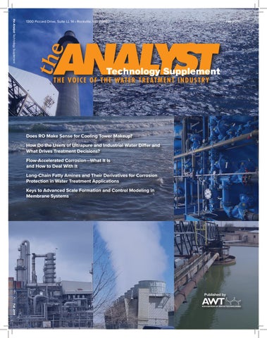
Does RO Make Sense for Cooling Tower Makeup? How Do the Users of Ultrapure and Industrial Water Differ and What Drives Treatment Decisions? Flow-Accelerated Corrosion—What It Is and How to Deal With It Long-Chain Fatty Amines and Their Derivatives for Corrosion Protection in Water Treatment Applications Keys to Advanced Scale Formation and Control Modeling in Membrane Systems
Published by Fall 2019
A COMPLETE SOLUTION
Designed to complete your water treatment system.
MicroVision EX makes life simpler for water treaters. Our advanced controller is easier to install, program and operate because of proven MicroVision software that utilizes an intuitive user interface. Accurate measurement is achieved by our toroidal probe, which is factory-calibrated and maintenance-free. And PULSAlink cloud-based communication delivers convenience at your fingertips with military grade, industry leading security. MicroVision EX controllers help maintain process control, reduce costs and limit downtime, freeing up more time for water treaters to serve their customers.
DON’T BOTHER WITH AN INCOMPLETE CONTROLLER. INSTALL THE MICROVISION EX FROM PULSAFEEDER.
Install Wizard.
Customization and Ultra-Secure.
Using the Install Wizard on all MicroVision EX controllers makes configuring installation, quick, easy, error proof, and customizable. Installs in less than five minutes.
Nameable relays, water meters, inputs, reports and customized color graphing. Ultra secure with the highest, industry leading AES256 encryption & TLS 1.2 protocol.
Improve ROI on Chemical Contracts.
PULSAlink Communications.
Corrosion Sensor.
High Pressure Applications.
MODBUS BMS Integration.
Right Out Of The Box.
Flow Meters with excellent precision and versatility, integrated with PULSAtron & MicroVision EX controller. Calculate and remotely track exact chemical dosed in the system minimizing loss and/ or overfeed.
Online corrosion monitoring to help water treaters track water quality and chemical treatment programs. Choice of 2 metal tips: Mild steel and Copper.
MicroVision Ex controllers equipped with an Ethernet interface can connect to a SCADA system via Modbus TCP communication protocol.
Web and iOS/Android App provides access to live reports, settings and notifications anytime,anywhere. Water meter plots include bleed, makeup and chemical totalization.
Models designed to withstand pressures up to 300 psi, where the cooling tower is on the top of a high rise building and the controller is in the equipment room many floors below/basement.
Making it simple to get everything you need in one location. The MicroVision EX can be ordered with Modem Millie installed on a choice of panels.
To learn more, contact your Pulsafeeder sales rep at pulsatron.com today!
rs. m re te is nk ur
ol, or
COVER Industrial plant in Texas (lower left corner). Photo courtesy of Charles Kuhfeldt.
Other photos: Ocean water by San Diego, California (middle left), power station smokestack (upper left), New York Bay water (upper right), IX treatment system at photovoltaic plant (middle right), power plant clarifier (bottom right), and power plant cooling tower (middle bottom). Photos courtesy of Mike Henley.
Fall 2019
Spotlight
Does RO Make Sense for Cooling Tower Makeup?....6
Long-Chain Fatty Amines and Their Derivatives for Corrosion Protection in Water Treatment Applications...................................................................40
James McDonald, Chem-Aqua While introduced as a water-saving alternative to once-through applications, cooling towers still use large volumes of water. As communities strive to conserve our natural resources, cooling towers are an obvious target for saving water in industrial, commercial, and institutional settings. How much water they use is based on many variables, but it could easily be 20% to 30% of a facility’s total water usage. Approaches to saving water in cooling towers focus on decreasing blowdown and, consequently, increasing the cycles of concentration. The focus of this article will be on using reverse osmosis (RO) for the removal/reduction of cycle-limiting components.
Klin Rodrigues and Fred Gadberry, AkzoNobel Long-chain fatty amines and their derivatives, sometimes referred to as filming amines, are widely used in the oilfield industry for corrosion protection. Oilfield applications typically involve acidic environments, in which these fatty amines are protonated and form a barrier on metallic surfaces. These molecules are finding increased use in water treatment applications. In contrast to most oil field applications, water treatment uses are typically on the alkaline side. Nevertheless, there are similarities in the film-forming mechanisms of these molecules and the insights gleaned from oilfield applications are applicable to water treatment applications.
How Do the Users of Ultrapure and Industrial Water Differ and What Drives Treatment Decisions?.......... 18
Keys to Advanced Scale Formation and Control Modeling in Membrane Systems.................................48
Mike Henley, M.D., Henley & Associates In the industrial world, it is common to hear the terms ultrapure water (UPW) or industrial water (IW). But what exactly is UPW? And, what exactly is IW? Is there one common water treatment method for all UPW? If not, why? This article will explore these questions and the elements that drive UPW treatment variations among different industries. It will also look at IW and technologies used to treat IW at industrial facilities. IW and UPW will be defined and the common treatment approaches for each category will be examined.
Robert J. Ferguson, French Creek Software, Inc. In the past, scale control in reverse osmosis (RO) was a straightforward process. Recovery rates were relatively low. Systems were operated with acid feed for pH control. And, in many cases, antiscalants were fed to provide a safety factor in the event of loss of acid feed. The evaluation systems for modeling scale were adequate for low-ionic-strength systems. Models based on the simple indices and calculations ceased to be applicable in the 1990s and began to be replaced by more sophisticated modeling algorithms. Modeling of treatment systems benefits from the incorporation of sophisticated calculation methods to improve accuracy and optimize treatment. This is of special applicability to 1) operating at higher RO recovery rates; 2) using seawater and reuse brines for feedwater; and 3) those operating in high ionic strengths. In this context, treatment optimization includes pH control and antiscalant dosages.
Flow-Accelerated Corrosion—What It Is and How to Deal With It.....................................................................34 Dennis McBride and Philip Walker, Burns & McDonnell A corrosion process referred to as flow-accelerated corrosion (FAC) has been determined to be the cause of multiple catastrophic failures in power plants, resulting in significant unplanned outages, expense, and even fatalities. By knowing where FAC can occur and using proper chemistry and metallurgical selections, these failures as well as future fatalities can be avoided.
3
the Analyst Technology Supplement 2019
1300 Piccard Drive, Suite LL 14 Rockville, MD 20850 (301) 740-1421 • (301) 990-9771 (fax) www.awt.org
2020 AWT Board of Directors President
Thomas Branvold, CWT
President-Elect
Michael Bourgeois, CWT
Secretary
Matt Jensen, CWT
Treasurer
Steven C. Hallier, CWT
Immediate Past President
David Wagenfuhr
Directors
Noah Baskin Mark Coldren, CWT Stephanie Keck, CWT Andy Kruck, CWT
Ex-Officio Supplier Representative
Garrett S. Garcia
Past Presidents
Brian Jutzi, CWT Jack Altschuler Bruce T. Ketrick Jr., CWT John Baum, CWT Bruce T. Ketrick Sr., CWT R. Trace Blackmore, CWT, Ron Knestaut LEED AP D.C. “Chuck” Brandvold, CWT Robert D. Lee, CWT Mark T. Lewis, CWT Brent W. Chettle, CWT Steven MacCarthy, CWT Dennis Clayton Anthony J. McNamara, CWT Bernadette Combs, CWT, James Mulloy LEED AP Alfred Nickels Matt Copthorne, CWT Scott W. Olson, CWT James R. Datesh William E. Pearson II, CWT John E. Davies, CWT William C. Smith Jay Farmerie, CWT Marc Vermeulen, CWT Gary Glenna Charles D. Hamrick Jr., CWT David Wagenfuhr Joseph M. Hannigan Jr., CWT Casey Walton, B.Ch.E, CWT Mark R. Juhl Larry A. Webb
Staff
Executive Director
Heidi J. Zimmerman, CAE
Deputy Executive Director
Sara L. Wood, MBA, CAE
Senior Member Services Manager
Calendar of Events Association Events 2020 Business Owners Meeting February 10–11, 2020 Hyatt Regency Clearwater Resort Clearwater, Florida
2020 Technical Training West
March 18–21, 2020 Marriott Cleveland Cleveland, Ohio
2020 Annual Convention & Exposition
September 30–October 3, 2020 Louisville Convention Center and Omni Hotel Louisville, Kentucky
2021 Annual Convention & Exposition
September 22–25, 2021 Providence Convention Center and Omni Hotel Providence, Rhode Island
2022 Annual Convention & Exposition September 21–24, 2022 Vancouver Convention Centre Vancouver, Canada
2023 Annual Convention & Exposition
October 4–7, 2023 Amway Grand Hotel and Grand Rapids Convention Center Grand Rapids, Michigan Also, please note that the following AWT committees meet on a monthly basis. All times shown are Eastern Time. To become active in one of these committees, please contact us at (301) 740-1421. Second Tuesday of each month
Angela Pike
Vice President, Meetings
East
February 26–29, 2020 Hyatt Regency Lake Washington Seattle, Washington
11:00 am
Legislative/Regulatory Committee
2:30 pm
Convention Committee
Grace L. Jan, CMP, CAE
Second Wednesday of each month
11:00 am
Business Resources Committee
Morgan Prior
Second Friday of each month
10:00 am
Special Projects Subcommittee
11:00 am
Cooling Subcommittee
Meetings Manager
Exhibits and Sponsorship Manager
Barbara Bienkowski, CMP
Exhibits and Sponsorship Associate Manager
Brandon Lawrence
Senior Marketing Director
Julie Hill
2:00 pm
Pretreatment Subcommittee
Third Monday of each month
9:00 am
Certification Committee
3:30 pm
Young Professionals Task Force
Third Tuesday of each month
3:00 pm
Education Committee
Third Friday of each month
9:00 am
Boiler Subcommittee
10:00 am
Technical Committee
11:00 am
Wastewater Subcommittee
Marketing Director
Jennifer Olivares
Technical Writer/Copy Editor Lynne Agoston
Accountant
Dawn Rosenfeld
The Analyst Staff Publisher
Quarterly (call for meeting dates)
Heidi J. Zimmerman, CAE
Managing Editor
Other Industry Events
Production Manager
• • • • •
Lynne Agoston
Jennifer Olivares
Technical Editor
Michael Henley (303) 745-3890, mdhenleywater@gmail.com
Advertising Sales
Heather Prichard, advertising@awt.org
The Analyst is published quarterly as the official publication of the Association of Water Technologies. Copyright 2018 by the Association of Water Technologies. Materials may not be reproduced without written permission. Contents of the articles are the sole opinions of the author and do not necessarily express the policies and opinions of the publisher, editor or AWT. Authors are responsible for ensuring that the articles are properly released for classification and proprietary information. All advertising will be subject to publisher’s approval, and advertisers will agree to indemnify and relieve publisher of loss or claims resulting from advertising contents. Editorial material in the Analyst may be reproduced in whole or part with prior written permission. Request permission by writing to: Editor, the Analyst, 1300 Piccard Drive, Suite LL 14, Rockville, MD 20850, USA. Annual subscription rate is $100 per year in the U.S. (4 issues). Please add $25 for Canada and Mexico. International subscriptions are $200 in U.S. funds.
ASHRAE, Winter Meeting, February 1–5, 2020, Orlando, Florida BOMA, Winter Business Meeting, February 2–5, 2020, Washington, D.C. CTI, Annual Conference, February 9–13, 2020, Houston, Texas NACE, Corrosion Conference & Expo, March 15–19, 2020, Houston, Texas ACS, Spring National Meeting & Expo, March 22–26, 2020, Philadelphia, Pennsylvania
4
the Analyst Technology Supplement 2019
President’s Message
By Tom Brandvold, CWT
The world of water treatment is vast, as evidenced by the breadth of articles in this Technology Supplement. As water treatment professionals, we all have our areas of subject matter expertise, but AWT’s Technology Supplement gives us the opportunity to be exposed to aspects of our industry we may not routinely encounter. Even if the treatment solutions aren’t ones we use every day, knowing the processes and chemistry behind them allows us to deploy effective solutions for our clients. Included in this Technology Supplement are articles about reverse osmosis for cooling tower makeup, ultrapure water, flow-accelerated corrosion, long-chain fatty amines, and scale control. This is great information for anyone involved in our industry. I hope you find this information helpful and that it adds value for your customers. As always, I welcome your feedback and can be reached at president@awt.org.
Editor's Notes
By Mike Henley water, which historically has been associated with the use of treatment chemicals.
Welcome to the 2019 fall Technology Supplement to The Analyst. This year’s theme focuses on the wide variety of water treatment that falls under the umbrella of “industrial water treatment.”
Robert Ferguson’s technical article examines a common concern in the operation of RO systems—membrane scaling. His discussion considers traditional approaches used to model scale formation and state-of-the-art calculation methods that overcome the limitation of earlier methods and can permit more accurate modeling in high-total dissolved solids waters.
Some of the inspiration for the theme hearkens back to the 1960s. Those of us of a certain age recall an era when televised sports lacked the bells and whistles of the digital technologies of 2019; the TV images were often fuzzy, and instant replays of athletic feats were not replayed over and over and over. During that period of time, the ABC network had a weekly sports anthology called The Wide World of Sports. This show explored sports dominated by individual athletes as well as the various team sports.
Differences Between Industrial and Ultrapure Water
In “How Do the Users of Ultrapure and Industrial Water Differ and What Drives Treatment Decisions?” I consider the differences between industrial waters and ultrapure waters (e.g., microelectronics, pharmaceutical, power plants). My article looks at how the water treatment standards differ and what will drive the use of specific treatment technologies.
The point? Successful industrial water treatment requires a wide variety of treatment technologies. Examples include chemicals, filters, activated carbon, membranes, ion exchange, electrodeionization, ozone, and UV. Laboratory services and monitoring technologies such as online instruments and colorimetric analysis provide the professional with the necessary tools to ensure that the treatment approaches are achieving the necessary water quality.
Corrosion Control
Klin Rodrigues, Ph.D., and Fred Gadberry, Ph.D., examine the use of filming amines for corrosion control in water treatment systems. These types of amines are popular for corrosion protection in oilfield applications and are finding greater use in water systems. Their article reviews different types of amines— monoamine, diamine, and triamine—and provides a technical explanation about each type.
Industrial and commercial water treatment covers a wide variety of applications. Each end-use application is unique and requires different approaches from the water professional’s tool box of treatment technologies. Hence, the title of the fall 2019 Technology Supplement: The Wide World of Water Treatment.
Authors Dennis McBride and Philip Walker discuss the phenomenon of flow-accelerated corrosion (FAC), which causes the preferential dissolution of the ferrous oxide (magnetite) layer on the inside of steam-cycle piping and equipment. This oxide layer is formed on the internal surfaces of piping and equipment as a result of steam-cycle water chemistries.
In this publication, we feature five technical articles that examine several topics important for the water treatment professional, including reverse osmosis, how different types of end-user applications differ, flow-accelerated corrosion, long-chain fatty amines, and scale control.
Reverse Osmosis
The danger of FAC is that it can weaken the tubes and piping in the high-pressure lines. The result is situations where piping or tubing can burst, which may force a plant to shut down for repairs. In extreme cases, an explosion may occur that can seriously injure or even kill plant workers.
James McDonald looks at the question of water conservation and whether or not it makes sense to use RO to help provide cooling tower makeup water. The article offers an interesting discussion on the possible merits for using RO for cooling tower
5
the Analyst Technology Supplement 2019
Does RO Make Sense for Cooling Tower Makeup? James McDonald, Chem-Aqua, Inc.
While introduced as a water-saving alternative to once-through applications, cooling towers still use large volumes of water. As communities strive to conserve our natural resources, cooling towers are an obvious target for saving water in industrial, commercial, and institutional settings. How much water they use is based on many variables, but it could easily be 20% to 30% of a facility’s total water usage.
and start to form scale and deposits within the water system, which can reduce heat transfer, increase corrosion, block flow, and negatively impact the system. It is typically the saturation limits of these nonvolatile components that limit how concentrated the water can be allowed to get as the cooling tower continues to evaporate water. The cycles of concentration refers to how many times the cooling tower water is concentrated compared to the makeup water entering the system to maintain the system water level. A common range is 4 to 6 in many areas. The cycles of concentration is controlled by wasting a portion of the concentrated water by blowdown (i.e., bleed).
Cooling towers achieve their temperature-reducing effect through sensible (direct contact) and evaporative cooling. On average, evaporative cooling is the primary driving factor. As water evaporates, it leaves the nonvolatile components in the water (e.g., calcium, magnesium, bicarbonate, chlorides) behind. Eventually, these components will reach their saturation limits
Equation 1 and Figure 1 show the overall mass balance around a cooling tower. Most of the makeup water requirements to a
6
the Analyst Technology Supplement 2019
cooling tower are to satisfy the evaporation demand, with blowdown being an ever-shrinking percentage as cycles of concentration are increased (as shown in Figure 2). While water treatment professionals typically have little to no control over the evaporation portion of the equation (which is determined by cooling load and current weather conditions), reducing the volume of blowdown may be within their control. Makeup = Evaporation + Blowdown
Eq. 1
Figure 1: Cooling tower mass balance.
It is assumed in Figure 1 that both controlled and uncontrolled water loses (e.g., leaks, drift, windage) are each included in the general “blowdown� variable. Figure 2 shows cooling tower water usage per 100 tons of cooling load.
Figure 2: Cooling tower water usage per 100 tons cooling load.
7
the Analyst Technology Supplement 2019
Does RO Make Sense for Cooling Tower Makeup? continued
Using RO for Cooling Tower Makeup
“While water treatment professionals
Does it make sense to use RO water for cooling tower makeup? The answer is “maybe,” but a mass balance around the entire water system must be considered, including both the RO and the cooling tower.
typically have little to no control over the evaporation portion of the equation (which is determined by cooling load and current
At first glance, it may seem that removing the cycle-limiting components of water (i.e., calcium, magnesium, and silica) would allow the cooling tower blowdown to be reduced to near zero as cycles of concentration are greatly increased. In reality, it does not always save water and can even use more. Only by calculating the mass balance can the user be sure. Let’s dig a little deeper into the idea of using RO for cooling tower makeup.
weather conditions), reducing the volume of blowdown may be within their control.”
Water-Saving Approaches
Approaches to saving water in cooling towers focus on decreasing blowdown and, consequently, increasing the cycles of concentration. The approaches fall into the following categories, as illustrated in Figure 3: •
Antiscalants (e.g., polymers, phosphonates, polyphosphates)
•
Removal/reduction of cycle-limiting components (e.g., water softeners, reverse osmosis)
•
Altering the water chemistry to increase solubility (e.g., lowering pH)
•
Filming of surfaces to inhibit scale buildup (e.g., filming amines)
•
Improved control (e.g., automatic online controllers)
•
Tightening up the system (e.g., fixing leaks, drift, windage, uncontrolled water loses)
•
Alternative makeup water sources (e.g., gray water, waste streams, reverse osmosis reject). While this may or may not actually save water usage within the cooling tower system itself, it may save water for the facility as a whole.
RO systems produce high-purity water by passing water through a semipermeable membrane. They are, however, limited by the same cycles of concentration concepts as cooling towers. The more concentrated the unwanted water components become (e.g., calcium, magnesium, silica), the greater the chance of forming scale on the membrane surfaces. Scaling can greatly reduce the ability of an RO to produce high-purity water and even lead to damage of the membranes themselves. Like in a cooling tower, a portion of the water is wasted to control how concentrated the water gets. This waste stream is called “concentrate” or “reject.” As Equation 2 and Figure 4 illustrate, the overall mass balances of both the RO and cooling tower are similar, with: •
Makeup supplying water
•
High-purity water leaving as permeate/evaporation
•
Concentrated waste streams leaving as reject/blowdown
Makeup = Permeate + Reject
Eq. 2
The focus of this article will be on using reverse osmosis (RO) for the “removal/reduction of cycle-limiting components.”
“Understanding that an RO can waste just as
Figure 3: Water-saving approaches for cooling towers.
or 5 cycles is important to note.”
much water as a cooling tower running at 4
8
the Analyst Technology Supplement 2019
with NorthQuest 599 See our NorthQuest offering at www.NorthQuest.US
North Metal & Chemical Co.
NorthQuest 599
excels at crystal modification, removing the flat surfaces that lead to scale NorthQuest 599 is a high performance terpolymer used as a scale inhibitor and dispersant.
BEFORE
Testing shows NorthQuest 599’s ability to act as a crystal modifier of CaCO3 lattice, and confirms its capacity as a sludge conditioning agent.
AFTER
Does RO Make Sense for Cooling Tower Makeup? continued
Figure 4: Reverse osmosis versus cooling tower mass balances.
Conventional ROs are typically designed to operate at 75% to 80% recovery. This means that 75% to 80% of the water going into an RO ends up as high-purity water (permeate) while 25% to 20%, respectively, ends up being wasted as reject water. How many times is the water within an RO concentrated? Using Equation 3, a 75% recovery RO operates at 4 cycles of concentration, while an 80% recovery RO operates at 5. See Table A for other comparisons. Cycles of Concentration = 1/ 1 – (% Recovery/100)
Eq. 3
Table A: % Recovery versus Cycles
Percent RO Recovery
RO Cycles of Concentration
75%
4
85%
6.7
80% 90% 95%
5
10
20
Understanding that an RO can waste just as much water as a cooling tower running at 4 or 5 cycles is important to note. Sure, the cooling tower may be able to theoretically run at much higher cycles, but if the pretreatment unit providing all the makeup is only running at 4 or 5 cycles, that is the BEST that can be achieved if the cooling tower blowdown were completely eliminated. Equation 4 and Figures 5 and 6 illustrate the overall mass balance of a cooling tower utilizing 100% RO makeup. Makeup = Evaporation + Blowdown + Rejection
Figure 5: Mass balance of using RO for 100% cooling tower makeup.
10
the Analyst Technology Supplement 2019
Eq. 4
Does RO Make Sense for Cooling Tower Makeup? continued
Figure 6: Cooling tower water usage per 100 tons cooling load, assuming 80% evaporative cooling and 10 ºF temperature drop.
Example of Using 100% RO for Cooling Tower Makeup Let’s illustrate this last point by considering the following cooling tower system. Table B lists the cooling tower blowdown and makeup requirements at various cycles. System conditions: •
Recirculation rate = 10,000 gallons per minute (gpm)
•
Temperature drop = 10 °F
•
80% evaporative cooling
•
Operating 24 hours a day, 365 days a year
Table B: Cooling Tower Water Requirements
Cycles
1.5
2
3
4
5
6
7
8
9
10
15
20
50
100
11
Makeup (gpm)
240
160
120
107
100
96
93
91
90
89
86
84
82
81
Evaporation (gpm)
80
80
80
80
80
80
80
80
80
80
80
80
80
80
the Analyst Technology Supplement 2019
Blowdown (gpm)
160
80
40
27
20
16
13
11
10
9
6
4
2
1
Does RO Make Sense for Cooling Tower Makeup? continued
As Table B shows, the cooling tower running at 5 cycles of concentration would require 100 gpm of makeup to replace the 80 gpm evaporation and 20 gpm blowdown. Looking at the extreme of 100 cycles of concentration, it would still require 81 gpm to replace the 80 gpm evaporation and 1 gpm blowdown. For comparison, Table C adds one more column showing how much water would need to be supplied to an RO system (running at 80% recovery) to supply the makeup required to a cooling tower at various cycles. Table C: Cooling Tower and RO Water Requirements
Cycles
Cooling Tower Makeup (gpm)
2
160
1.5
240
3
120
5
100
7
93
4
6 8
107
80 80
86
133
13
80
10
113
80
6
107
2
102
80
84
80
100
81
80
82
27
80
20 50
200
20
80
15
300
80
80
80
91
89
160 40
80
90
Cooling Tower Blowdown (gpm)
100% RO Makeup @ 80% Recovery (gpm)
80
96
9
10
Cooling Tower Evaporation (gpm)
80
150
125
16
120
11
114
9 4
1
117
Table C clearly illustrates that even at the extreme of 100 cycles, the overall RO-cooling-tower system uses MORE makeup water than a cooling tower running at 5 cycles of concentration without RO makeup (at 80% recovery). Why is this? Remember from Table A that an RO running at 80% recovery is already cycling the water five times in the reject stream. Before the RO permeate even makes it to the cooling tower, it has already wasted as much water as if the cooling tower had achieved 5 cycles of concentration by itself. If the cooling tower has any blowdown at all, it uses more. Figures 7 and 8 illustrate this example. A cooling tower running by itself at five cycles without RO makeup and using standard chemistries, high-stress chemistries, or pH control would have saved more water than having to invest the capital funds and annual operational costs of the RO system.
111
105 101
Figure 7: Example of cooling tower mass balance at 5 cycles of concentration.
12
the Analyst Technology Supplement 2019
Legionella
Laboratory
Indoor Air Quality
ONLYYOU CAN PREVENT LEGIONNAIRES' DISEASE
Environmental Safety Technologies Leading the way in Legionella testing since 1993...
• Legionella & Pathogen Testing • Detailed Legionella Laboratory Reports • Standard 7-10 Day and 96 Hour Rapid Turn-around • Emergency Outbreak Response The EST Team consists of a diverse group of professionals:
• Ph.D. Microbiologist • Certified Water Technologist • Certified Industrial Hygienist • Certified Indoor Air Quality Professional • Certified Healthcare Contractor • Certified Indoor Environmental Consultants • Laboratory Analysts • Environmental Specialist • Project Managers We pride ourselves on being competitively priced, offering personalized customer service that is flexible and responsive to our customers' needs.
Call us today to learn more about other waterborne pathogens.
•Pseudomonas•Acinetobacter•Burkholderia•Stenotrophomonas•NTB-Mycobacterium•Fungi Serving Customers Throughout North America
www.estechlab.com I 502-893-6080 I est@estechlab.com ��rK I Department of Health
�ATE
ELAP No. 12068
Does RO Make Sense for Cooling Tower Makeup? continued
Figure 8: Example of cooling tower mass balance with RO makeup and 100 cycles of concentration.
If the cooling tower had originally been running at less than five cycles, then water savings are theoretically possible. As Table C shows, a cooling tower system requires 107 gpm makeup at four cycles of concentration without RO makeup. With RO makeup at 80% recovery, the system only needs 101 gpm at 100 cycles as an extreme. The question to be asked is if an RO can run at 80% recovery (i.e., five cycles) if the cooling tower itself could only run at four cycles of concentration without RO. Since ROs are often limited by the same scale-forming species as cooling towers, additional pretreatment, such as water softening, may be required. Then softener regeneration waters must be factored into the mass balance.
How Many Cycles Can a Cooling Tower Run?
Running a cooling tower at 100 cycles is typically not possible because of leaks, windage, and drift, among other factors. Often, 10 to 20 cycles of concentration are found to be the maximum a cooling tower can physically achieve, and sometimes even less. This makes the comparison to using RO even worse. As Table C shows for an 80% recovery RO, running the cooling tower at 20 cycles equates to running the cooling tower without RO at between four to five cycles. At 10 cycles, this equates to between three to four cycles. Using an RO with 75% recovery makes the example even worse (e.g., running a cooling tower at 20 cycles with RO makeup equates to running a cooling tower without RO makeup at between three and four cycles). Table A is more telling than first implied because even at nearly infinite cycles, a cooling tower system with 100% RO makeup will NEVER use less water than a cooling tower system with-
out RO makeup running at the same cycles of concentration as the RO itself (e.g., at 80% RO recovery and infinite cycles, the system will use the same amount of makeup as a cooling tower at five cycles of concentration without RO makeup).
“…even at nearly infinite cycles, a cooling tower system with 100% RO makeup will NEVER use less water than a cooling tower system without RO makeup running at the same cycles of concentration as the RO itself.”
Unconventional ROs
We’ve been basing our assumptions on conventional RO designs that typically achieve 75% to 80% recovery, depending upon the makeup water quality. There are unconventional designs, such as reverse-flow and closed-circuit systems, that may achieve greater percent RO recoveries (90% to 98%) by taking advantage of the short residence time of the water within the RO versus the induction time for scaling to occur. Such systems also do not have to deal with higher temperatures of heat exchange surfaces that drive scale formation that must be accounted for with cooling tower systems. There are other high-recovery, patented RO designs available for reduction of cycle-limiting component such as silica. 14
the Analyst Technology Supplement 2019
Does RO Make Sense for Cooling Tower Makeup? continued
Using our example of a cooling tower running at five cycles of concentration again, adding an RO for 100% makeup running at 90% recovery could potentially use less water if the cooling tower cycles could be pushed over nine cycles, as the tables in the next section will show.
Table D: Break-Even Cycles of Concentration Using 75% Recovery RO
% Blend Old Cycles of Concentration
Blended RO Makeup
When 100% RO makeup is not a viable option based upon the mass balance or other reasons, perhaps a blend of RO permeate and another source should be considered. Blending RO water with city, soft water, or other sources may reduce the offending component limiting cooling tower cycles. Examples include:
1.5
•
10
2
•
Silica reduction may reduce the potential for silica deposits.
•
Chloride reduction may reduce the corrosion potential for stainless steel components.
•
Total hardness reduction may reduce the potential for scale formation in systems with high skin temperatures at heat exchange surfaces.
4
75%
100%
1.57
1.64
1.71
1.80
3.60
4.50
6.00
9.00
New Minimum Cycles of Concentration to Break Even using an RO with 75% Recovery
5.33
5
7.50
40.00
15
NA
20
NA
50
NA
100
NA
2.40
2.67
8.00
16.00
15.00
NA
NA
NA
NA
NA
NA
NA
NA
NA
NA
NA
3.00 NA NA NA NA NA NA NA
Table E: Break-even Cycles of Concentration Using 80% Recovery RO
% Blend
As already discussed, and based on mass balance calculations, what would be the new cycles of concentration at which the blended-RO-makeup-water system would need to operate to truly save water? The math can be complicated, but Equation 5 and Tables D, E, F, and G show the break-even points. Running at cycles of concentration above those calculated or shown will start saving water, assuming the cooling tower water chemistry allows the cooling tower to run at such cycles.
Old Cycles of Concentration 1.5 2 3 4
5
10
15
20 50 Eq. 5
50%
2.18
3
Alkalinity reduction may reduce the need to feed acid and/ or minimize white rust formation.
25%
100
25%
50%
75%
100%
1.55
1.60
1.66
1.71
3.43
4.00
4.80
6.00
New Minimum Cycles of Concentration to Break Even using an RO with 80% Recovery 2.13 4.92
6.67
22.86
120.00 NA NA NA
2.29 6.40
10.00 NA NA NA NA NA
2.46 9.14
20.00 NA NA NA NA NA
Where: CyclesOld = Previous cycles of concentration with 0% RO makeup CyclesMin = Minimum cycles of concentration required when using RO water to break even with water usage of CyclesOld at various percent blends % Blend = Percent of RO water in blended cooling tower makeup water % Recovery = RO design percent recovery
15
the Analyst Technology Supplement 2019
2.67
16.00 NA NA NA NA NA NA
Does RO Make Sense for Cooling Tower Makeup? continued
Table F: Break-Even Cycles of Concentration Using 85% Recovery RO
% Blend Old Cycles of Concentration 1.5 2 3 4 5
10
15
20 50
100
25%
50%
75%
100%
1.53
1.57
1.61
1.65
3.29
3.64
4.08
4.64
New Minimum Cycles of Concentration to Break Even using an RO with 85% Recovery 2.09 4.61
6.07
16.59
39.23
123.64 NA NA
2.19
5.44 7.73
48.57 NA NA NA NA
2.31
6.63
10.63 NA NA NA NA NA
2.43
8.50
17.00 NA NA NA NA NA
Table G: Break-Even Cycles of Concentration Using 90% Recovery RO
% Blend Old Cycles of Concentration 1.5 2 3 4 5
10
15
20 50
100
25%
50%
75%
100%
1.52
1.54
1.57
1.59
3.18
3.38
3.60
3.86
New Minimum Cycles of Concentration to Break Even using an RO with 90% Recovery 2.06 4.36 5.63
13.33 24.55
42.35 NA NA
2.12
4.80 6.43
20.00 67.50 NA NA NA
2.18
5.33 7.50
40.00 NA NA NA NA
2.25 6.00 9.00 NA NA NA NA NA
Accurately blended water can be a challenge to achieve. Will it be done by throttling valves, volumetrically, or some other method? Taking the time to engineer a reliable system is vital to such a program’s success.
RO Pretreatment
is desired, one must always do an overall mass balance to determine if water usage is truly reduced. Other reasons include: Reusing RO water. RO permeate that is too contaminated from its original use (e.g., rinse water) could potentially be used for cooling tower makeup, depending upon the contaminants. Recovering wastewater. Using RO to recycle wastewater back to the cooling tower may be a possibility in water-stressed areas or where company or governmental policy mandates it. Using the proper pretreatment steps ahead of the RO is important (e.g., filtration, clarification, ultrafiltration, microfiltration, nanofiltration, disinfection). Excess RO capacity. RO systems may be overdesigned due to future plans or reduced need, or to meet peak demand. With the desire to keep the RO systems running to reduce up and down times and stagnant conditions, the plant may produce more RO water than can currently be used. This may be a candidate for cooling tower makeup, with a backup plan for when RO water is not available.
Using RO’s Other Water: Reject
An RO may be producing high-quality permeate for another application, but the RO reject could still be of high enough quality to use for cooling tower makeup, particularly if the makeup water to the RO is softened. This has the benefit of using water that ordinarily would have been sent to the drain. It is important, of course, to consider the impact of RO reject on the overall cooling water chemistry. Can the RO reject provide 100% makeup or just a portion? Will the RO reject be collected in a storage tank? What happens when the RO is down? Will a backup soft water source be required? Is the RO close enough to the cooling tower to make it logistically possible? If the RO reject is blended with other makeup water sources (e.g., city water), how will this affect solubilities of calcium and other factors? Will acid feed be required to reduce alkalinity and pH? Will the cycles of concentration of other components, such as silica and chlorides, be an issue?
Other RO Makeup Considerations
While this article has focused on mass balances, the need for economic and energy balances should not be forgotten. The total cost of operation of an RO system must be considered in addition to any water saving benefits (if any). Factors may include:
The above discussion assumes there are no RO pretreatment water losses. If a water softener is used, for example, the regeneration wastewater will need to be factored into the overall mass balance as well. If a filter is used, the backwash water must be accounted for and will negatively impact the overall water savings.
•
Capital costs
•
Electricity
•
Membrane replacement
•
Cleaning
Mass Balance and Beyond
•
Routine maintenance
•
Antiscalant
•
Dechlorination
There are other reasons and schemes for using RO for cooling tower makeup, not all of which save water. When water savings
16
the Analyst Technology Supplement 2019
Does RO Make Sense for Cooling Tower Makeup? continued
•
Microbiological control
“It is important to know the overall water
•
RO reject destination
•
Softener costs
mass balance and take into account all the
•
Other Pretreatment costs (e.g., carbon filters, macro filtration, ultrafiltration)
•
Footprint required for system installation
As cycles of concentration increase in a cooling tower system, the holding time index (HTI) increases as well. This means that whatever is in the cooling tower water will stay in the cooling tower water longer before leaving the system. This may impact the effective lifespan of corrosion inhibitors, antiscalants, and dispersants. Cooling towers also function as air scrubbers, removing pollen, blossoms, dirt, and dust from the surrounding air. This may require sidestream filtration to keep the system clean. The backwash water from any filtration system will need to be considered in the overall mass balance. Corrosion control may need to be a consideration. Water is the universal solvent, and high-purity water can increase corrosion potential. Is it cheaper to treat for corrosion or scale? Is blended water an economical option for corrosion control? When using RO for boiler makeup, the fuel savings typically make the scheme economically favorable. Considering these other considerations with RO for cooling tower makeup, however, economics and practical aspects may outweigh any advantages of water savings.
factors to make an informed decision instead of falling for a mirage.”
Conclusion
Using RO for cooling tower makeup may be a great solution or may not be. Does the treatment scheme really save water? Does it save or cost more money? It is important to know the overall water mass balance and consider all the factors to make an informed decision instead of falling for a mirage of water savings. James McDonald, PE, CWT, is the technology and marketing manager at Chem-Aqua, Inc. He is the current chair of the AWT Certification Committee and incoming chair of the AWT Technical Committee. Mr. McDonald is the 2013 winner of the AWT Ray Baum Memorial Water Technologist of the Year Award. He has published numerous industrial water treatment papers in trade journals and has written the book Drop by Drop: Articles on Industrial Water Treatment. He is also the founder of Industrial Water Week, an annual global, grassroots, open-source celebration of the noble profession of industrial water treatment held during the first full business week of October.
The ability to control the cooling tower itself cannot be forgotten. Is the current controller working properly? Are probes regularly maintained, calibrated, and replaced? Are dosing pumps in working order and maintain prime? The higher the cycles of concentration in a cooling tower system, the higher the reliability of control needs to be for when things go wrong. A little bit of hardness getting to the system, for example, will be amplified at higher cycles. Is the cooling tower itself maintained to minimize uncontrolled water losses? Tracing down piping and referring to updated piping diagrams may be required to hunt down water loses. Water flow may need to be balanced over the distribution decks to prevent water from splashing onto the ground. Drift eliminators and fill may need to be replaced. Lastly, using RO as makeup to a cooling tower system is not likely to eliminate the need for adding water treatment chemicals. The system may still need dispersants, antiscalants, corrosion inhibitors, and microbicides.
17
the Analyst Technology Supplement 2019
How Do the Users of Ultrapure and Industrial Water Differ and What Drives Treatment Decisions? Mike Henley, MD Henley & Associates
18
Photo courtesy of Micron Technology, Inc.
the Analyst Technology Supplement 2019
Abstract
In the water world, the terms “ultrapure water” (UPW) and “industrial water” (IW) have different meanings, depending on the application. Essentially, each water name acts as an umbrella term for several types of water.
treatment approaches for each category. In the final part of the article, we will spell out some of the organizations whose work influences water treatment decisions. The aim of the author is to provide an overview with appropriate research tools for those who wish to pursue the subject in a deeper, more technical fashion.
In UPW, there are really three primary categories: semiconductor water, pharmaceutical water, and power water for suband super-critical boilers. Each kind requires specific types of treatment to ensure they meet the specifications for use in their respective end use. Likewise, on the IW side, there really are several categories, including pulp and paper, boiler water, petrochemical plants, oil refineries, and general industrial.
In the next section, we begin by providing some definition of what constitutes UPW and IW. It should be noted that, while each category has unique purification requirements, ultimately they are two general facets of water treated at industrial facilities. First, we will examine UPW.
What is UPW?
For example, in the production of microelectronics water, the goal is a final water quality with a resistivity around 18.2 megohm-cm (at 25 °C). To achieve this quality of water, a facility will use treatment technologies such as ion exchange (IX), reverse osmosis (RO), electrodeionization, ultrafiltration, microfiltration, ozone, and UV. Additionally, great care is given to the choice of materials of construction for piping and valves. Whether one is thinking of UPW or IW, one important factor that impacts the water treatment decisions are the different published guidelines. The list of organizations reads like alphabet soup: ASME, ASTM, EPRI, IAPWS, SEMI, and pharmacopeias (USP, JP, EP). Through the use of data (charts and tables) and practical information, the aim of this article is as follows: 1. To provide a breakdown on what the umbrella terms UPW and IW mean; 2. To examine how water treatment varies and is similar between and within the two categories; 3. To briefly highlight the organizations that develop the standards used by different end user industries and the role each plays; and 4. To help readers come to a clearer understanding about these differences and their impact on water treatment decisions.
Introduction
Water. That simple word conveys a complex topic that represents the very essence of life—we enjoy its beauty in nature and also drink it and use it for cooking, bathing, and household cleaning. In the bigger picture, water provides countless jobs because it is the key cog for many industries— power generation, semiconductor and pharmaceutical manufacturing, and industrial plants. In addition, water is important for process and comfort cooling and plays a critical role in mining and oil and gas exploration. In the industrial world, it is common to hear the terms ultrapure water or industrial water. But what exactly is UPW? And, what exactly is IW? Is there one common water treatment method for all UPW? If not, why? This article will explore these questions and the elements that drive UPW treatment variations among different industries. We will also look at IW and technologies used to treat IW at industrial facilities. We will define IW and UPW in the first section of this article and then examine the common
UPW is also called “high-purity water,” but for the purposes of this article, we will use the term UPW. The three main industrial users of UPW are the microelectronics, pharmaceutical, and power generation industries. We will refer to each category as a separate grade of UPW. We will explore the unique requirements for each category, but first, it is important to note that to ensure the necessary level of purity, end users commonly use online instruments to measure for water conductivity, or its reciprocal, resistivity. As noted by Gray (1), conductivity and resistivity readings are a simple way to indicate the level of water purity. They also are a basic data point for indicating a problem with the treatment system. Because the microelectronics industry seeks water that is free of any contaminant (dissolved or suspended), it uses resistivity and considers a resistivity of 18.2 megohm-cm at 25 °C to meet its specification for semiconductor-grade water. Other industries use conductivity and consider a reading of 0.0550 microsiemens per centimeter (μS/cm) at 25 °C as pure water. Table A (2, 3) offers a comparison between the comparative conductivity and resistivity readings at 25 °C for different types of water. Table A: Conductivity and Resistivity Readings for Different Water Qualities at 25 °C
Water Type UPW (microelectronics) Power plant boiler water Pharmaceutical water* Distilled water Deionized water Demineralized water Mountain water Drinking water
Conductivity 0.055 µS/cm
Resistivity 18.2 megohm-cm
0.05–1.0 µS/cm
1–20 megohm-cm
1.3 µS/cm
0.77 megohm-cm
0.5 µS/cm 0.1–10 µS/cm 1–80 µS/cm
2.0 megohm-cm 10–0.1 megohm-cm 1–0.01 megohm-cm
10 µS/cm
0.1 megohm-cm 0.1–1 millisiemens/cm 1–2 kiloohm-cm
Sources: Reference 2, Van London (n.d.). *Data based on Reference 3, USP 40 (2017).
From Table A, the conductivity and resistivity requirements for semiconductor UPW (18.2 megohm-cm) are significantly different from what is needed for pharmaceutical water (1.3 µS/cm 19
the Analyst Technology Supplement 2019
How Do the Users of Ultrapure and Industrial Water Differ and What Drives Treatment Decisions? continued
conductivity) and power plant boiler water (0.05 to 1.0 µS/cm conductivity). These data points illustrate the water-quality differences for what are often considered the three classes of UPW. In fact, the author has learned that it is more accurate to refer to each particular water quality based on the overall end use. The term “UPW” really is an umbrella term for a class of industrial waters that share some similarities related to their production and ultimate purity characteristics. So, we will now first explore these three categories of UPW. In our discussion, we will also highlight treated water uses and quality requirements. Then, we will take a shorter look at some of the key types of industrial water. Figure 1 provides a simple illustration of the industries considered to use UPW. Figure 1. Primary types of UPW end-user industries.
-
Important uses for semiconductor-grade water include rinsing to clean chemicals used on microchips during the different production steps. Examples would involve the rinsing of etchants from photolithography steps and as a rinse from chemical-mechanical planarization processes. UPW is also used as an ingredient in some chemicals used for microchip production.
Pharmaceutical-Grade Water
Ironically, pharmaceutical water is less pure than that used by the microelectronics industry. This is true, even though pharma water is the basis for the different medicines doctors may prescribe, as well as the intravenous fluids that have saved many lives in emergency rooms and hospital beds. Pharmaceutical-grade waters consist of 10 different types of water. The most basic type is Purified Water. From there, facilities produce other grades, based on the products they are manufacturing and the water-quality standards. The different types of pharmaceutical water include Bacteriostatic Water for Injection, Purified Water, Sterile Purified Water, Sterile Water for Inhalation, Sterile Water for Injection, Sterile Water for Irrigation, Water for Injection, Water for Hemodialysis, Pure Steam, and Highly Purified Water. These various types of water have different end uses in plants. Applications include pharmaceutical production steps; as an ingredient; and for bottle/container rinsing, equipment cleaning/ sanitization, floor mopping, and washing products (e.g., healthcare devices). Pharmaceutical-grade waters are primarily used in pharmaceutical and biopharmaceutical plants; however, their uses also extend to the manufacture of healthcare devices and into the life sciences to produce consumer products (toothpaste, mouthwashes, and others) and cosmetics. Essentially, pharma water is used whenever the production protocol calls for the use of pharmaceutical-grade water. We shall examine this area more closely in the next section of the article.
Power Plant Water Semiconductor-Grade Water
Of the three main types of UPW, water used in microelectronics is considered to have the highest purity, with a resistivity of 18.2 megohm-cm. The industry’s water experts will refer to this water as either ultrapure water, UPW, or semiconductor-grade water. For this paper, we will use the latter term. Semiconductor-grade water is used in plants that make semiconductors, flat-panel displays, and photovoltaic panels. This semiconductor water is considered water that has been treated to the highest purity standards for the removal of different types of contaminants, including organic and inorganic compounds, dissolved and particulate matter, volatile and nonvolatile, reactive and inert, and dissolved gases (4). Semiconductor water treatment follows three steps: pretreatment, the main purification system, and polishing steps to ensure the water purity prior to use in the facility.
In the water treatment world, power plants fall under two general categories: conventional and nuclear generating stations. Both categories use boilers for steam to drive the turbines. Now, we will briefly look at these two categories of power stations. Conventional plants. At one time, this category was broadly associated with coal-fired facilities, but in the past couple decades that has changed with the growth in natural gas as a fuel source and the decline in the number of coal stations. Natural gas fueled stations include combined-cycle plants that have heat recovery steam generators (HRSG). Not all power plant water fits under the category of UPW. Boilers that are rated as super-critical and sub-critical require high-purity boiler feedwater. Briefly, here are short overviews on these two types of boilers (5):
20
the Analyst Technology Supplement 2019
How Do the Users of Ultrapure and Industrial Water Differ and What Drives Treatment Decisions? continued
•
•
Super-critical boilers are usually found at power plants generating at least 400 megawatts (MW). These boilers usually operate at pressures of 3,500 pounds per square-inch gauge (psig) (24.1 megapascal [MPa]) or more, and steam temperatures in the 1,100 °F (595 °C) range. Sub-critical boilers pressures are usually from 1,800 to 2,600 psig (12.4 to 17.9 MPa) at 374 °C. As needed, the superheater and reheater outlet temperatures often are in the range of 1,000 to 1,050 °F (538 to 566 °C).
Please note that at these pressures and temperatures, the water quality is critical to protect against turbine scaling and boiler tube scaling and corrosion that, under extreme conditions, can cause boiler and turbine failures. Nuclear. Likewise, nuclear plants use steam to make electricity. Two main categories of nuclear plants are pressurized water reactors (PWR) and boiling water reactors (BWR). In each case, high-purity water is needed as a reactor cooling stream and as a boiler feedwater. The heated cooling water will go to a heat exchanger where it heats the boiler feedwater to product steam to drive the turbines. Please note, some nuclear stations use material other than water as the reactor cooling agent. Because of the concerns about plant safety, great care is taken in the treatment of nuclear power plant water to protect against corrosion and scaling. In plants that use water for reactor cooling, the heated water will then go through a heat exchanger to heat boiler feedwater to create steam to drive the turbines. Much more could be said about nuclear power plant water, but the aim of this paper is to provide an overview.
process. Oil refineries also have brine desalter wastewater and stripped sour water (SSW) treatment, and petrochemical facilities have treatment of spent caustics. The close observer will also note that at a certain point, a UPW plant’s water quality degrades and must be treated as an industrial wastewater, or as necessary, treated for reuse. In addition, whether a facility produces microchips or automobiles, UPW and IW plants both will have cooling water systems used with process streams or for heating, ventilation, air conditioning (HVAC) purposes. The overall distinction between IW and UPW is that the waters treated by industrial users do not need to meet the same purity levels as required in UPW facilities. However, care still must be taken when treating IW because there is equal concern that the process streams do not cause defective products or worse, cause a boiler explosion or steam pipe rupture that, if catastrophic, will kill workers and cause plant shutdowns. And, in some applications, there is a concern on the IW side that the water does not have microbiological contamination. Table A also shows the range of conductivity levels IW users would aim for—particularly for power generation boilers—and deionized water that would be used in lower-pressure boilers and other process streams.
Figure 2. Primary types of IW end-user categories.
-
What Is Industrial Water?
In this section, we will examine some of the variations on the IW side. As is true for the UPW side, the IW side really is a collection of different industries using treated water in their plants. Those industrial users include petrochemical, petroleum (upstream, mid-stream, and downstream), pulp and paper, steel and other metals, heavy and light industrial plants, and mining. Power generation is also part of this category for plants with less than sub-critical boilers, which at lower pressures do not require the same high-purity water treatment. Included in the power category would be natural gas cogeneration plants, captive plants (for industrial users), and peaking plants. Figure 2 provides a simple breakdown of types of IW end users. As can be seen in the figure, IW consists of a number of categories, many of which use boilers and process water. Because these boilers have lower pressures, they do not require the same water purity as super and sub-critical boilers. Other types of IW can include process waters used in facility operations and treated waters for products such as those made by beverage companies. Additionally, coal-fired power plants often use water as a part of their flue gas desulfurization (FGD)
Types of IW Users
When thinking of IW end users, the universe is essentially all other types of plants outside of those using some type of UPW. Briefly, here are some examples:
Boiler Water
This type of water treatment covers many industrial categories listed here: • • • • 21
Power plants with boilers under 900 psig Pulp and paper mills Petrochemical plants Oil refineries the Analyst Technology Supplement 2019
How Do the Users of Ultrapure and Industrial Water Differ and What Drives Treatment Decisions? continued
• • • • • •
Steel and metals Food and beverage Heavy oil recovery by steam assisted gravity drainage (SAGD) boilers Manufacturing Institutions Light industrial and commercial applications
Industrial boilers have many uses. One common purpose is to produce steam for use in industrial processes such as petrochemicals and oil refineries. Another is to drive turbines used in captive power plants that serve a manufacturing facility. Boilers are also used to provide steam for heating or hot process waters for use in industrial or commercial processes.
Other Treated Waters
The following are some brief examples of other treated IW streams. Process water. Likewise, industrial plants need treated water for their manufacturing processes, such as washing or heating and cooling. For the latter two cases, the water streams will pass through a heat exchanger to reach the temperature needed for the industrial process. Food and beverage. This industry treats water for use as an ingredient in its products or for washing fruits and vegetables before final processing. Specialty wastewater treatments. Though different from traditional wastewater treatment, IW also entails treatment of waste streams from FGD in power, spent caustic (petrochemical), and stripped sour water (refineries). These categories really involve processes to clean wastewater streams.
ing the treated water. We shall now briefly explore water quality and end-user needs, beginning with UPW.
UPW
Microelectronics plants. Our discussion will primarily focus on the semiconductor industry, but the water-quality concerns held by semiconductor plants are shared by the flat-panel display industry and photovoltaic solar plants. Overall, microelectronics plants literally seek to produce the highest purity water because of concerns that the water may contribute to product defects with the microchips produced by the plants. As noted earlier, resistivity is a good basic monitoring technology because it can confirm that treatment systems have done their jobs and that the water meets the quality standards as indicated by Wikipedia (4). The microelectronics industry has seen major advances in the product technologies manufactured by companies in the industry. For example, microchips have gotten significantly smaller. A simple example is the small SD card put in cell phones to expand storage space. Today, a 64 gigabyte (GB) card far exceeds the original memory cards used in the first digital cameras. Those first digital camera cards were even considered “large” if they could hold 256 megabytes (MB). Figure 3 shows a size comparison between an SD card such as used for supplemental memory in cell phones and a Zip disk. The Zip disk has a capacity of 100 MB while the SD card (center of Zip disk) can hold up to 64 GB of data. In its day, the Zip disk was considered innovative because, compared to the old floppy disks and the 3.5-inch disks, it was capable of storing significantly more data. However, CDs and DVDs soon superseded it. Figure 3. Zip disk that could hold 100 MB of data and a 64-GB SD card used in cell phones (center of Zip disk).
In the next part of this article, we will examine some of the common treatment technologies found in IW. This will come after our discussion about UPW treatment approaches.
Water Treatment Technologies
Now, we take time for a Captain Obvious statement: “Treatment technologies used in industrial plants are influenced by the final quality needed.” While that is plain, it is still worth examining so that one can understand what influences water treatment in different types of industrial facilities. As in the first section, we will begin with UPW and then examine IW.
What About UPW Treatment Practices?
As discussed and illustrated in Figure 1, UPW really refers to industries that each require varying purities of high-purity water. It is at this point that the types of treatment technologies vary by industry and are determined in part by the end-user water-quality requirements and treatment guidelines/standards unique to each industry. Ultimately, the manufactured product deeply influences the treatment needs and, in turn, the technology. In most cases, the treatment guidelines are based around a facility successfully us-
As Figure 3 simply illustrates, the semiconductor industry’s technology revolution has sharply changed the physical characteristics of microchips and other products and has meant a necessary revolution in water-quality requirements. At one time, the line widths on chips were measured in the micron range. But, the newest chips have line widths that are narrower than 22
the Analyst Technology Supplement 2019
SUPPLIER OF THE YEAR
Bringing Quality Blending To The West Coast QualiChem is proud to announce the opening of our new
No Direct Sales
precision blending facility in Verdi, Nevada. We are now
Precision Manufacturing
better positioned to provide our customers with industryrecognized benefits and services coast to coast. Just one more way we are demonstrating how‌
The Blender Matters 800.296.9102 | www.qualichem.com AN ISO 9001:2015 COMPANY
Formulatory Expertise Application Support Custom GHS-Compliant Labels and SDSs
How Do the Users of Ultrapure and Industrial Water Differ and What Drives Treatment Decisions? continued
a human hair and measured in nanometers (nm). The industry is also beginning to make new chips that are three-dimensional. The consequence is that these latest products require even purer water and that particles even as small as 10 nm need to be removed. Particles are removed by filtration, but they are measured by instruments. On the monitoring side, fabs want particle measuring instruments to accurately measure under 20 nm. The concern about particles is that they can land on a microchip line during cleaning steps and potentially cause a product failure. Similar concerns are held about dissolved solids, which could precipitate onto a microchip electrical line and be the source of a product defect. As noted in Wikipedia (4), semiconductor plants have sophisticated water treatment systems. They also take water-quality monitoring seriously and not only measure for resistivity, but also for total organic carbon (TOC), particles, pH, and specific ionic contaminants (e.g., boron) in plant water. Materials of construction is an important requirement in a microelectronics plant. One common example is polyvinylidene fluoride (PVDF), which is used for piping systems, storage tanks, and valves and fittings (6). PVDF is seen by the industry as an inert material that will not leach or shed contaminants (particles) into the water. Municipal water is a common feed source for most microelectronics fabs. Pretreatment before the main treatment system is determined by the level of suspended solids and organics in the source water. Common pretreatment steps include multi-media filtration and ultrafiltration and activated carbon for organics and chlorine removal. This is then followed by some type of reverse osmosis (RO). The primary treatment will include ultraviolet light (UV) for organics reduction followed by electrodeionization (EDI) and/or mixed-bed ion exchange (IX) for deionization. There can also be a step to remove dissolved oxygen by degasification membranes or vacuum degasification. The final step is polishing that includes UV, heat exchange for controlling a constant temperature in the UPW supply, non-regenerable IX, membrane degasification, and ultrafiltration (UF) for particle control. In some cases, a fab may practice point-ofuse (POU) filtration. Table B provides an overview of some water guidelines for semiconductors, which is based on the F63 guidelines developed by SEMI’s Liquid Chemicals Global Technical Committee (7).
Table B: Overview of Semiconductor Water Guidelines
Parameter Resistivity TOC (online for < 10 ppb Silica (total and dissolved) Online dissolved oxygen Nonvolatile residue Bacteria
Semiconductor UPW 18.2 megohm-cm <1 µg/L 0.5 µg/L 10 µg/L 0.1 µg/L <1 cfu/100 mL
Note: Particle measurement is not included in this table because updated guidelines are still being developed by water experts involved with SEMI and the IRDS. The other listed guidelines are also subject to updating.
Semiconductor water standards. In the microelectronics industry, water-quality guidelines are developed by water experts involved with SEMI’s Liquid Chemicals Committee. SEMI is an industry trade group that represents the global microelectronics industry. SEMI’s Liquid Chemicals Committee has task forces that work on different aspects of water treatment and components used to produce semiconductor-grade water. The SEMI expert groups work in conjunction with the IRDS (International Roadmap for Devices and Systems). Two examples of water standards issued by SEMI are F61—“Guide to Design and Operation of a Semiconductor Ultrapure Water System” and F63—“Guide for Ultrapure Water Used in Semiconductor Processing.” These and other standards are updated regularly. It is important to note that the guidelines issued by SEMI are voluntary in nature and are not mandated by any government agency. They are widely followed, but manufacturers may also have customized standards they follow.
Pharmaceutical/Life Sciences
As noted, pharmaceutical water includes 10 categories that are defined by the United States Pharmacopeia (USP) and other major pharmacopeias (European Pharmacopeia [EP] and Japanese Pharmacopeia [JP], among others). The basic grade is Purified Water (PW), which is used for cleaning and as an ingredient for some pharmaceutical and consumer products. However, many products and manufacturing processes require even purer water. Hence, different classes of waters are produced to meet the specific requirements needed for making pharmaceuticals and life sciences products. Table C (4) provides examples of some grades of pharmaceutical water and their final uses.
24
the Analyst Technology Supplement 2019
How Do the Users of Ultrapure and Industrial Water Differ and What Drives Treatment Decisions? continued
Table C: Examples of Uses for Pharmaceutical Waters
Water Type Water for Injection (WFI) Bacteriostatic WFI Sterile Water for Irrigation Sterile WFI Sterile Water for Inhalation
Source: Reference 4.
Application Used for bulk preparation of medicines for parenteral administration. Also can be used for container washing and cleaning in highly sterile production areas. Used for ophthalmic and multiple-dose injections. Used as a diluent for internal irrigation therapy products. Used in injections. Used as a diluent for inhalation therapy products.
Facilities making pharmaceutical water are required to begin with a water quality that meets the U.S. Environmental Protection Agency’s Drinking Water Standards. So, if the feedwater source is not from a municipal drinking water plant, then it is necessary to treat the incoming water. The feedwater is then treated by technologies such as activated carbon, ultrafiltration, and microfiltration before going to RO and IX or EDI. Other common treatments include UV and ozone. Heat sanitization is commonly achieved with hot water. This water is then considered PW, provided it meets the quality standards as set by the pharmacopeias. To qualify as Water for Injection (WFI), however, which is considered the purest grade of pharmaceutical water, it must undergo further treatment to ensure the water is sterile and free from microorganisms (e.g., bacteria, viruses, fungi) or endotoxins. The conventional approach used to achieve this water quality is by distillation. However, now the USP, EP, and JP also permit the use of membrane technologies as part of a treatment system used to achieve WFI without the use of distillation. The EP just began allowing this treatment approach in 2017 (8). Table D (9) summarizes some treatment standards for PW and WFI.
Table D: Highlights of Pharmaceutical Water-Quality Standards
Parameter
USP Limits
Total Aerobic Microbials (cfu/mL)
100
TOC (mg/L)
0.5
Purified Water
Conductivity (µS/cm at 25°C) Water for Injection
1.3 (3 stage).
Total Aerobic Microbials (cfu/mL)
10
TOC (mg/L)
0.5
Conductivity (µS/cm at 25°C)
Bacterial Endotoxin (EU/mL)
1.3 (3 stage) 0.25
Note: Other pharmacopeias can have requirements on ‘ other parameters. Source: Based on table in Reference 9, p. 5 (2017).
Pharmaceutical industry water regulations are determined by regional pharmacopeias, of which the EP, JP, and USP are the key players, although the Chinese Pharmacopeia (CnP) and the Indian Pharmacopeia (IP) are gaining influence. Unlike the SEMI guidelines, the pharmacopeias are the basis for government regulation and enforcement action for noncompliance. In the United States, the U.S. Food and Drug Administration enforces the water-quality standards developed by the USP. In the case of the USP, a water experts committee works in conjunction with USP staff to develop and update regulations. The USP is a private organization based in Rockville, Maryland, which started in 1820. Later in the 1800s, the U.S. Congress passed legislation that gave the standards developed by the USP the standing of law. The USP has nine water monographs and five key general chapters. A monograph is a legal definition for a particular type of water. Two key monographs published by the USP are “Purified Water” and “Water for Injection”. The water-related chapters include the following: <645> Water Conductivity, <643> Total Organic Carbon, <1231> Water for Pharmaceutical Purposes, <1644> Theory and Practice of Electrical Conductivity Measurements of Solutions, and <1231> Water for Hemodialysis Applications (10). The USP has a five-year cycle in which its different standards and guidance documents are reviewed and updated as necessary.
Power
Power stations treat boiler feedwater to make steam for making electricity. This is true for all thermal plants—whether they burn coal or use natural gas, nuclear, or other energy sources. As noted earlier, facilities using sub- and super-critical boilers must meet stricter quality standards as set by the International Association for the Purification of Water and Steam (IAPWS). The American Society of Mechanical Engineers (ASME) also develops guidelines for boilers, and the Electric Research Power Institute (EPRI) works with its members to publish guidance documents for different aspects of boiler water. For the very high-pressure boilers, common treatment technologies used after pretreatment can include reverse osmosis followed by ion exchange or EDI. Vacuum degasification or degassing membranes will be used for oxygen removal, although some power plants now actually oxygenate their water to control corrosion. Condensate polishing with either powdered IX resin filters or IX vessels is also practiced by some plants. In pharmaceutical water and semiconductor water, the treatment regimens aim to avoid any use of treatment chemicals. However, in power plants, the high water and steam temperatures affect metallurgy and water chemistry. Therefore, power stations also treat their water with chemicals or adjust water chemistry to prevent scaling and corrosion in boiler systems and on the turbine blades. One example is the use of filming amines to protect against corrosion in the water-steam cycle. 25
the Analyst Technology Supplement 2019
How Do the Users of Ultrapure and Industrial Water Differ and What Drives Treatment Decisions? continued
Table E (9) provides a summary of guidelines from IAPWS and EPRI on steam purity and makeup water. Table E: Summary of Recommended Guidelines for Steam Purity, Makeup Water
Parameter Conductivity Cation conductivity Silica Sodium Chloride pH Dissolved oxygen
IAPWS 3-5 µS/cm <0.20 µS/cm <10 ppb <2 ppb <2 ppb 9.1-9.3 < 10 ppb
Source: Summary of table in Reference 9, p. 9 (2017).
Power industry treatment standards. As referenced earlier in this section, the IAPWS plays a key role in the treatment guidelines used for treating water at power stations. Through its website, the organization offers Technical Guidance Documents (TGD) that may be downloaded. These TGDs are followed by power stations globally (11). In addition to IAPWS, other organizations (e.g., ASME, EPRI, ABMA) and manufacturers like Babcock & Wilcox provide guidelines on boiler operation.
Treatment Technologies
Table F (12) provides an overview of the different treatment technologies used by the power, pharmaceutical, and microelectronics industries.
Table F: Overview of Technologies Found in Different UPW Treatment Applications
UPW Water Users Microelectronics (semiconductors, flat panel display, solar)
Relevant Treatment Technologies A, B Pretreatment: multi-media filtration (MMF), diatomaceous earth (DE), activated carbon filtration (ACF), ultrafiltration (UF), microfiltration (MF), cartridge filters Main: IX, RO, EDI, UF, MF, UV POU: IX, vacuum degasification (VDG), membrane degasification (MDG), HX, UV, UF Other: Monitoring instruments such as pH, TOC, conductivity, particle counters, resistivity, temperature, pressure, flow, DO, H 2O2, O3, other specialty ion (e.g., boron) instruments; sanitization systems (ozone, UV); hot DI heaters.
Pharmaceutical/Biopharmaceutical* Healthcare Devices**, Cosmetics***, Consumer Products***
Materials of construction are critical for system components—piping, valves. Mostly consists of PVDF, PFA, PTFE, limited use of 316L SS. Incoming feedwater meets EPA Drinking Water Standards (NPDWR). Pretreatment primarily aims at chlorine removal by carbon or metabisulfite. Main treatment technologies employed can include IX, RO, MF, UF, UV, ozone, EDI, and distillation.
*Product Water or for those requiring water for manufacturing and/or cleaning. Sterilization/sterility may be required for packaged products or for final product quality. **Products that require water in the pro- Note: Materials of construction are a critical consideration, often stainless steel for hot water sanitization. duction process or for cleaning. *** Products that require water as an ingredient in the production process or for cleaning. Power Plants with super-critical or sub-critical boilers (fossil, combined cycle, nuclear)
Wastewater: Treatment techniques are generally limited to pH adjustment, so maintenance items such as RO membrane cleaning are either outsourced or the membranes are discarded. Pretreatment, IX—primary and polishing, RO, EDI, UF, MF, condensate polishing Other: Oxygen removal (e.g., hydrazine); FGD; service (drinking) water; wastewater; in some cases—oxygenated treatment Monitoring: pH, conductivity, TOC, other specialty monitors as needed.
Specialty (e.g., labs, university research facilities)
Note: Nuclear plants can have needs unique to them in their water system. Often smaller-scale treatment systems. Features may include service DI, smaller EDI, RO, monitoring instruments, etc.
Source: Table compiled by Henley, Reference 12. Notes: A The technologies listed for each end user category are examples of what is commonly found. However, local water quality can affect decisions about treatment technologies. B The treatment technologies listed are for the UPW water used by end user facilities. The technologies listed do not consider treatment for process waste streams or cooling water.
26
the Analyst Technology Supplement 2019
How Do the Users of Ultrapure and Industrial Water Differ and What Drives Treatment Decisions? continued
What About IW Treatment Practices?
On the IW side, many of the same treatment technologies are used; only the end users’ water quality needs are less than needed for UPW. Table G (13) provides an overview of treatment technologies common to different IW end users. The brief summaries that follow provide basic information about organizations involved with developing treatment guidelines for users of UPW. Table G: Overview of Technologies Found by Industrial Water Treatment Type
Industrial Users Power Generators*: Traditional fossil Integrated Gasification Combined Cycle Gas Turbine Combined Cycle General Industry (captive power plants) * Pulp & Paper Oil Refining: Downstream (refining & petrochemical) Mining (Ore concentrate) Metal Processing: Metal (steel mills, aluminum, copper) Food Processing/Beverage Desalination for mining, power, industrial end uses General Manufacturing (e.g., automotive, plastic molding) Chemical Manufacturing Commercial/Institutional (e.g., universities, hospitals, large commercial buildings) Emerging/Developing Market Opportunities: Waste-to-Energy* Biofuel Processing
Relevant Treatment Technologies Pretreatment: multimedia, filters, deaeration activated carbon Main: IX, condensate polishing, RO, EDI, softening, and chemicals for scale and corrosion control. Other: Monitoring instruments such as pH, conductivity (specific and cation), silica, ORP, sodium, and TOC Similar technologies as used with power boilers; lime and lime-soda ash softening. Similar technologies as used with power boilers Pretreatment, RO, IX Specialty chemicals, RO, IX Disinfection, UV, ozone, RO, IX, GAC Pretreatment filtration, RO desalination IX, RO, boiler and steam/condensate chemical treatment Similar approaches as used with power boilers Pretreatment, Softening, IX, RO Similar technologies as used with power boilers Similar technologies as used with power boilers
Source: Henley, Reference 14. Note: * Includes facilities that may have boilers used for combined heat and power production.
Boiler Water
As noted in Table F, common treatments associated with power plants include IX, condensate polishing, softening, and specialty chemicals. The chosen treatment technologies are based around the boiler pressure. For example, under-300 psig, simple water softening, or even chemical treatment for a high-quality water source could be sufficient for a boiler feed. On the other hand, a high-pressure (HP) boiler needs a pure water, as noted by Boyd (14). For the HP unit, RO and IX would be likely primary treatments for the boiler feedwater. Wong (15) notes that membrane technologies are increasingly being found in boiler water treatment, often in conjunction with IX. As Table F lists, industrial boilers in other applications also need similar treatment technologies. One important consideration is the materials of construction used in a boiler’s water-exposed surfaces. Because of the high heat and boiler pressures, chemical treatments such as amines, ammonia, all-volatile treatments, hydrazine, and others are used to protect metals against scaling and corrosion. The decisions are based around metal alloys and the boiler pressure. Table H (16) gives one example from an ASME document (17) of how some selected parameters in treated boiler feedwater can vary for different pressure boilers.
27
the Analyst Technology Supplement 2019
How Do the Users of Ultrapure and Industrial Water Differ and What Drives Treatment Decisions? continued
Table H: Examples of Boiler Feedwater Treatment Requirement Variations
Operating Pressure (psig) Feedwater Dissolved Oxygen (before scavenger) (mg/L) Total Iron (mg/L) Total Copper (mg/L) Total Hardness (mg/L) pH (at 25°C)
Source: ASME, Reference 16.
0–300 psig
451–600 psig
751–900 psig
1001–1500 psig
<0.007 ≤0.1 ≤0.05 ≤0.3 8.3-10.0
<0.007 ≤0.03 ≤0.02 ≤0.2 8.3-10.0
<0.007 ≤0.02 ≤0.05 ≤0.1 8.3-10.0
<0.007 ≤0.01 ≤0.01 ND 8.3-9.6
Other Waters
In the food and beverage industry, a key concern is ensuring that the water has no harmful microorganisms. Therefore, disinfection is an important consideration through treatments like UV and ozone. Treatment technologies such as RO, IX, and GAC are common. In the automotive industry, DI water is used in the painting process, and it is important that when dried, there are no water spots. Table I (17) provides an overview of different treatment concerns within IW users. Note that, in addition to pure water areas, other concerns by industrial plants relate to water reuse and different aspects of wastewater treatment for pollution control (e.g., FGD, spent caustic, turbine injection water, tailing waters). Table I: Overview of Industrial Water Treatment Areas
Industrial Users
Power Generators*: Traditional fossil Integrated Gasification Combined Cycle Gas Turbine Combined Cycle General Industry (captive power plants) * Pulp & Paper Oil Refining: Upstream Mid-stream Downstream (refining & petrochemical) Mining (Ore concentrate): Copper Iron Aluminum Coal Metal Processing: Metal (steel mills, aluminum, copper) Food processing/ Beverage
Cooling Water
ZLD
Reuse
Ash Pond or Tailing Pond Effluent
X X
Makeup Water**
Non-PowerProducing Boilers***
Condensate Polishing****
X X
X X
X X
Towers
Blowdown FGD
Industrial Wastewater
X X
X X
X X
X X
X X
X X
X
X
Note A
X
X
X
X
X
X
X
X
X
X
X
X
X
X
X
X
X
X
X
X
X
X
X
X
X X X
X
X X X
X X X X
X X X X
X X X X
X X X X
X X X X
X
X
X
X
X
X
Notes B, C
X
X
X
X
X
X
X
X
28
SAGD X
the Analyst Technology Supplement 2019
X
X
How Do the Users of Ultrapure and Industrial Water Differ and What Drives Treatment Decisions? continued
Table I: Overview of Industrial Water Treatment Areas, continued
Industrial Users
Desalination for mining, power, industrial end uses General Manufacturing (e.g., automotive, plastic molding) Chemicals Commercial/Institutional (e.g., universities, hospitals, large commercial buildings) Emerging/Developing Market Opportunities: Waste-to-Energy* Biofuel Processing
Source: Henley, Reference 17.
Cooling Water
Ash Pond or Tailing Pond Effluent
Makeup Water**
Non-PowerProducing Boilers***
Towers
Blowdown FGD
Industrial Wastewater
X
X
X
X
X
X
X X
X X
X X
X X
X
X X
X X
X X
X X
X X
X X
X
X
X X
ZLD
X X
Reuse
X
X
Condensate Polishing****
General Comments: Local water-quality conditions do vary and will affect the degree and sophistication of treatment methods required to successfully treat the water, as outlined in this table. While the end uses for the treated water vary, treatment approaches for each of these categories are often similar between industries for the different categories of water use. Notes: * Includes facilities that may have boilers used for combined heat and power production. ** Can involve different treatment technologies such as softening, ion exchange, reverse osmosis. This water may be used as a boiler feedwater, or may be the make-up water to a plant process that requires water. *** Reverse osmosis and ion exchange are the typical process for makeup water production in even the highest-pressure boilers, including supercritical. Boilers under 900 psig can perhaps be fed with ion-exchange water or just two-pass RO alone. **** Not always practiced. A: Gas turbine injection water for nitrogen oxide control. B: Oil refineries have brine desalter wastewater and stripped sour water that requires treatment. C: Petrochemical plants treat spent caustic.
Who Provides Treatment Guidance?
Here is a list of some of the organizations that help to develop documents that provide guidance on the treatment of UPW and IW.
ABMA
The American Boiler Manufacturers Association (ABMA) is based in Vienna, Virginia. It publishes its own resources related to boiler operation and also works with AHRI (Air Conditioning, Heating, and Refrigeration Institute), ASME (American Society of Mechanical Engineers), the National Board of Boilers and Pressure Vessel Inspectors, and NFPA (National Fire Protection Association) in the development of codes and standards.
ASME
The ASME, based in New York, provides guidance documents for a number of industrial areas. Related to power, the ASME’s work involves boiler water, feedwater, and pressure vessels.
ASTM
The American Society for Testing and Materials International (ASTM or ASTMI) is based in West Conshohocken, Pennsylvania. The organization has committees that develop consensus-based standards for a variety of subject areas. The Committee D-19 on Water develops standards on different aspects of water treatment.
AWT
The Association of Water Technologies (AWT) is based in Rockville, Maryland. The organization has published the Technical Reference and Training Manual and the Raw Materials Specifications Manual, both of which are resources for learning about water treatment technologies and standards that impact the industry. Both manuals are being updated.
29
the Analyst Technology Supplement 2019
How Do the Users of Ultrapure and Industrial Water Differ and What Drives Treatment Decisions? continued
CTI
The Cooling Technology Institute (CTI) is a member-led trade organization whose work has included the development of guidelines for cooling water treatment.
EPRI
The Electric Power Research Institute (EPRI), based in Palo Alto, California, is an organization that conducts research in different aspects of power generation, including those involving the use of water.
IAPWS
International Association on the Properties of Water and Steam (IAPWS) is an international association of national organizations concerned with the properties of water and steam. A primary area of concern is thermal power and other industrial and scientific applications. The IAPWS has committees that have subject matter experts who work to develop guidelines on cycle chemistry and technology for steam power in fossil and combined-cycle plants.
ISPE
The International Society of Pharmaceutical Engineers (ISPE), based in Bethesda, Maryland, is a trade organization that represents the interests of the pharmaceutical industry, including water treatment. ISPE's work includes committees that have published books related to pharmaceutical water treatment. One recent example is the Good Practice Guide: Approaches to Commissioning and Qualification of Pharmaceutical Water and Steam Systems. These documents are developed by industry experts and are designed for use by water system operators in the pharmaceutical and life sciences industries.
Closing Thoughts
The term UPW does not refer to a universal water-quality standard or treatment approach because each end user category has different needs. Rather, a more appropriate way to view UPW is that it represents an overall type of water treatment where the users require a highly pure water to achieve their goals. Purposes for the water may include steam for the generation of electricity, the production of pharmaceuticals and healthcare products, the manufacture of microchips or photovoltaic panels, or for research and other specialty applications. Likewise, IW represents a water treatment category with different quality standards based on the final need. Additionally, for each type of UPW and IW, there are professional organizations or industry groups that help to develop guidelines for the water treatment needs.
Acknowledgements
The author wishes to express deep gratitude to Dr. Frank Slejko, the founder of Ultrapure Water Journal, for the many opportunities he provided the author to learn about different aspects of the water treatment industry. The author also is grateful for the following individuals who have willingly shared their knowledge and helped review tables prepared by the author that are included in this article: Anthony Bevilacqua, Ph.D., Mettler-Toledo Thornton; Slava Libman, Ph.D., FTD Solutions; Brad Buecker, ChemTreat; Joseph Manfredi, GMP Systems; William V. Collentro, Pharmaceutical Water Specialists, LLC; David Daniels, M&M Engineering Associates Inc.; the late Paul Puckorius, Puckorius & Associates; Dan Wilcox, Samsung; Avijit Dey, Ph.D., Jacobs; and Ted Beardwood, Solenis.
PDA
The Parenteral Drug Association (PDA) is based in Bethesda, Maryland. It was founded by a group of pharmaceutical manufacturers in 1946. One aspect of the PDA’s work involves developing documents on different aspects of the manufacture of parenteral drugs, including areas that touch on water treatment.
SEMI
SEMI (formerly known as Semiconductor Equipment and Materials International), based in Milpitas, California, represents the global semiconductor industry. As a part of its work, SEMI develops guidelines on different aspects of semiconductor manufacture, including water treatment guidelines.
USP
The United States Pharmacopeia (USP) is based in Rockville, Maryland. It provides information on different aspects related to pharmaceutical manufacturing, including water treatment.
30
the Analyst Technology Supplement 2019
How Do the Users of Ultrapure and Industrial Water Differ and What Drives Treatment Decisions? continued
References 1. Gray, D.M. (2015, January/February). Backgrounder: Why does conductivity matter? Ultrapure Water Journal 32(1). 14-16.
2. Van London (n.d.). Education Series: Conductivity Guide. Van London-pHoenix Co., Phoenix, AZ. Retrieved from: www.vl-pc.com. 3. USP 40. (2017). Physical Tests. <645> Water Conductivity. United States Pharmacopeial Convention Inc. Rockville, MD.
4. Wikipedia. (n.d.). Ultrapure water. Retrieved from: https://en.wikipedia.org/ wiki/Ultrapure_water.
5. Babcock & Wilcox Co. (n.d.). Boilers and steam generation for power, renewable and industrial applications. Babcock & Wilcox Co. Barberton, OH. Retrieved from: http://www.babcock.com/en/technology/steam-for-power-process. 6. Burkhart, M.; Mueller, H.; Trinkner, M.; Williamson, C. (2013, May/June). 450-mm PVDF pipe and fittings production to accommodate the UPW volume demands of future megafabs. Ultrapure Water Journal 30(3). 16-25. 7. SEMI. (2016). Based on guidelines developed by SEMI’s Liquid Chemicals Global Technical Committee. F63 guide for ultrapure water used in semiconductor processing. Available at: www.semi.org. 8. Henley, M. (February 2017). What water treatment advancements mean for pharma. PDA Letter. 26-28.
9. Mettler-Toledo Thornton. (2017). Pure water guide: regulations and standards overview for water purification. Mettler-Toledo Thornton. Billerica, MA. Retrieved from: www.mt.com. 5, 9.
10. Henley, M. (May 2016). Is a revolution needed in water treatment technologies? Interview with Dr. Anthony Bevilacqua. GWI | Ultrapure. Available at: www. ultrapurewater.com. 11. Dooley, B. ( June 2018). Personal communication with Barry Dooley, Ph.D., International Association on the Properties of Water and Steam.
13. Henley, M. (2018b). Table on overview of technologies found by industrial water treatment type. MD Henley & Associates, Denver, CO.
14. Boyd, W. (2015, September-October). In what ways do chemical treatments differ for high-pressure boilers when compared to lower-pressure boilers? Ultrapure Water Journal 32(4). 11-14.
15. Wong, J. (April 2017). What are useful membrane technology applications for power plant water treatment and reuse? GWI | Ultrapure. Available at: www. ultrapurewater.com.
16. ASME. (2001). Consensus on the operating practices for the control of feedwater and boiler water in modern industrial systems. ASME. New York, NY.
17. Henley, M. (2018c). Overview of the industrial water marketplace. MD Henley & Associates, Denver, CO.
Mike Henley currently serves as a water industry consultant through MD Henley & Associates. He also is the technical editor for The Analyst, a journal published by the Association of Water Technologies. Mr. Henley previously served for 27 years as the editor of Ultrapure Water Journal. Among his duties was helping to organize the technical programs for the ULTRAPURE WATER Conferences. This paper was originally presented at the International Water Conference, which was conducted on November 4–8, 2018, in Scottsdale, Arizona. More information is available at www.eswp.com/water.
12. Henley, M. (2018a). Table on technologies found in different UPW treatment applications. MD Henley @ Associates, Denver, CO.
31
the Analyst Technology Supplement 2019
Flow-Accelerated Corrosion— What It Is and How to Deal With It Dennis McBride, Burns & McDonnell, and Philip Walker, Emerson
34
the Analyst Technology Supplement 2019
Abstract
A corrosion process referred to as flow-accelerated corrosion (FAC) has been determined to be the cause of multiple catastrophic failures in power plants, resulting in significant unplanned outages, expense, and even fatalities. By knowing where FAC can occur and using proper chemistry and metallurgical selections, these failures as well as future fatalities can be avoided.
Figure 1: Solubility of magnetite as a function of temperature at various ammonia concentrations.
Flow-Accelerated Corrosion
Flow-accelerated corrosion (FAC) is the preferential dissolution of ferrous oxide (Fe3O4, magnetite) that generally had been formed to protect steam cycle surfaces from other forms of corrosion. Iron (Fe), by its nature, prefers to be in an oxide form. The formation of oxides to provide a layer resistant to further corrosion is called passivation. Steam cycle chemistries historically have used chemical addition (oxygen scavengers and amines) to create reducing environments with mildly alkaline pH, allowing magnetite to preferentially form, which provides a relatively passive protective layer on the internal surface of the piping or equipment. This process is shown graphically in the Appendix, Figure A-1 (Iron Oxidation in a Reducing Environment). Magnetite is relatively porous and soluble under certain conditions that can often be found in steam cycles. These conditions include: •
Relatively low, albeit still alkaline, pH levels.
•
A reducing environment.
The porous nature of the magnetite allows for water to migrate through the oxide layer to the metallic iron surface, which encourages further oxidation to occur. The oxidation process is an equilibrium reaction and is normally inhibited once the oxide is formed due to reduced diffusion of reactants and products through a fluid boundary layer that forms along the water/metal junction. Any action that reduces this fluid boundary layer (e.g., flow turbulence), however, reduces this natural reaction inhibition and can allow the oxidation to continue to destructive levels. The solubility of the magnetite can also disrupt the protective oxide layer by reducing the thickness of the layer, allowing for the oxidation process to continue. This solubility reaches a peak at temperatures often found in steam cycles (e.g., feedwater economizers, heater drains). Figure 1 (1) graphically indicates the solubility as a function of temperature.
Source: EPRI, Reference 1.
FAC can occur in both in a single-phase (water only) or twophase (water and steam) environment. In traditional fossil plants, conditions allowing for single-phase FAC include the boiler feedwater sections of the cycle. Two-phase FAC can typically be found in feedwater heaters, drain lines, and deaerators. In combined-cycle plants, FAC has typically occurred in the low-pressure (LP) evaporator circuits, although incidents are known to have occurred in the intermediate-pressure (IP) and high-pressure (HP) economizer or preheater tubing. Figure 2 (1) indicates the typical areas of concern for a heat recovery steam generator (HRSG) system. Figure 2: Schematic of typical FAC locations in an HRSG.
Source: EPRI, Reference 1.
History of FAC
FAC has caused failures throughout the power industry over the years, but in the past, the cause of the failures was almost always unknown or unreported. This changed, however, when a high-pressure condensate line in the Surry nuclear plant ruptured in 1986. This event caught the attention of the media, 35
the Analyst Technology Supplement 2019
Flow-Accelerated Corrosion—What It Is and How to Deal With It continued
particularly because the incident killed four people and injured four more (2, 3). Several other incidents have shone light onto the problem of FAC, particularly incidents involving nuclear plants. The incident that brought the focus on FAC into the power industry in general, rather than just nuclear plants, was the Pleasant Prairie fossil plant failure (1). This accident resulted in the deaths of two plant supervisors and occurred despite having corrosion inspection programs in place (4). As news of these failures emerged, researchers began to search for the cause of this mechanism. It was soon discovered that the reducing program, common to steam cycles at that time, was a contributor to the failure in many of the FAC incidents. Investigators determined that with operation in a reducing environment, within a pH range common to steam cycle operations, the protective layer of magnetite lining the pipes and boilers would dissolve, leaving the bare metal exposed (5). This led to rapid degradation and corrosion of the piping and equipment in many power plants. The reduced metal wall thickness could reach a point where it could no longer contain the system pressure, causing the plant to fail and resulting in the deaths of workers in some cases. Due to this discovery, power plants have implemented corrosion prevention policies and inspection requirements to prevent future accidents (2). In addition, newer plants have been moving away from reducing treatment programs and finding oxidizing alternatives such as all volatile-oxidizing AVT(O) and oxygenated treatment (OT) (5). FAC is a well-understood mechanism today, and power plants have programs in place to help prevent accidents from occurring in the future.
Addressing FAC
There are generally three industry accepted methods to address potential FAC issues. •
Higher oxidation potential
•
Higher pH
•
Metallurgical choices
Higher oxidation potential. In systems that are all-ferrous materials (condenser may contain copper alloys), EPRI has provided guidelines for an AVT(O) feedwater treatment that requires a small residual of oxygen to be maintained. Generally, the residual oxygen remaining in the deaerated condensate (e.g., 5 to 10 parts per billion [ppb]) will be adequate. Further mechanical or chemical deaeration is not required or recommended. By creating an oxidizing environment, the formation of ferric oxides and hydroxides is encouraged. These are significantly less soluble than the ferrous oxides formed in the traditional reducing environment (see Appendix, Figure A-2 Iron Oxidation in an Oxidizing Environment). The ferric salts therefore form a more persistent passive layer with the resultant reduction in corrosion
rates. Figure 3 (1) indicates this relative solubility of the ferrous and ferric salts. Figure 3: Relative solubility of ferrous and ferric salts.
Source: EPRI, Reference 1.
Note: The top line, indicating Fe2O4 Solubility Field should read Fe3O4. In combined-cycle systems, the use of oxidizing environment alone is not recommended, as the low-pressure (LP) drum will act to deaerate the feedwater (distribution ratio at LP conditions approximately 1000:1 oxygen in steam compared to boiler water, see Appendix, Figure A-3) prior to its use in the high and intermediate pressure systems. During boiling in the LP drum, the majority of the ammonia is also volatilized and lost in the LP saturated steam. The graph in Appendix A-3 indicates the distribution ratio (i.e., the quantity of a chemical species found in the steam versus in the water phase). Ammonia has a distribution ratio of approximately 10 (10 times more ammonia in the steam than in the water) at typical LP drum conditions. It is common for the LP drum “blowdown” to form the feedwater for the intermediate-pressure (IP) and high-pressure (HP) sections of an HRSG, which means this stream will have only about 10% of the ammonia of the LP feedwater. pH being a logarithmic scale means the IP/HP feedwater will have a pH about one unit lower than the LP feedwater. Oxygen content decrease from the LP to the IP/HP feedwater streams will be even more dramatic, with oxygen distribution ratio being about 10,000 to 1. Due to the loss of ammonia and oxygen in the LP drum, using the correct metallurgy in the downstream systems is critical to preventing FAC. While IP/ HP feedwater failures are less frequent in FAC cases, these failures pose much more risk and must be accounted for with proper metallurgy. Metallurgical choices are discussed at length later in this article. Higher pH. The second method of addressing FAC, a higher pH, promotes the formation of the ferrous/ferric hydroxide passive layer by providing more hydroxide ions in the form of ammonium hydroxide. Since copper alloys are subject to corrosion by ammonia, the AVT(O) feedwater treatment does not allow for the use of copper alloys in the condensate and feedwater sections of the cycle (use of copper alloys in the condenser 36
the Analyst Technology Supplement 2019
Flow-Accelerated Corrosion—What It Is and How to Deal With It continued
is allowed). If copper alloys are present in the condensate or feedwater sections, EPRI provides guidance for operation in a reducing environment, AVT(R), but this program does not provide the added FAC control of the AVT(O) program. The lower iron solubility at increasing pH is shown in Figure 4 (1). Figure 4: Projected iron concentration versus water pH.
used to monitor the potential for FAC occurrence. Included in this inspection plan should be all areas of the system that are susceptible to FAC. Inspections should be done at least on an annual frequency. For sections of the steam cycle that may be subject to two-phase FAC, the issue must be addressed through metallurgical selection as chemical remedies (i.e., oxygen and ammonia) will always concentrate in the gas phase and not help to mitigate the corrosion.
Conclusions
Source: EPRI, Reference 1.
Metallurgical choices. As mentioned previously, oxygen levels maintained in the condensate system will mostly be lost to the LP steam (HRSG) system because of deaeration, and they are not available to assist in the passivation of carbon steel surfaces in the feedwater system. The environmental condition in between the LP drum and the other drums makes this section of the combined cycle particularly susceptible to FAC. The environmental conditions consist of the following: •
Lower oxygen levels
•
Temperature in the FAC range of 100 to 300 ºC
To protect this particular section of the system, the piping should be made of an FAC-resistant alloy. EPRI recommends steel alloys containing chromium ≥ 1.25% (e.g., P11 or P22), although alloys with chromium contents as low as 0.1% have shown significant protection from FAC. The effect of the chromium content on the mitigation of FAC is indicated in Figure 5 (6).
FAC is a phenomenon that is fairly unique to the steam generation process. FAC has been identified as one of the leading causes of failures in steam generators and has resulted in significant issues, such as unscheduled shutdowns and even the death of several operators. There are two forms of FAC, single-phase and two-phase, each of which must be addressed in a different manner. The means to address this issue involve chemistry (pH, oxidation-reduction potential) and metallurgical considerations. Implementing an oxidizing program is instrumental in addressing the water chemistry concern, resulting in the formation of ferric oxide within the iron oxide matrix. This ferric oxide is significantly less soluble than the ferrous oxides formed in a reducing environment, providing for a more stable passive surface and thus, less corrosion. The oxidizing programs accomplish this through dosing ammonia for pH control and maintaining dissolved oxygen residual. To address metallurgical concerns, steel containing a minimum of 0.1% chromium should be used in areas that cannot be adequately protected chemically. With these measures in place, FAC will be significantly reduced and future catastrophic failures averted.
Appendix
Figures A-1 (1) and A-2 (2) illustrate the differences in iron oxidation in a reducing environment (A-2) and an oxidizing environment (A-2). Figure A-1: Iron oxidation in a reducing environment.
Figure 5: Chromium effect on FAC resistance.
Source: EPRI, Reference 1. 1 Fe = Fe2+ + 2e 2 H O + 2e - = 2 OH- + H 2
Source: EPRI, Reference 6.
In systems where the choice is to use steel material that is not resistant to FAC, it is recommended that an inspection plan is
2
2 Fe + + OH - = Fe(OH)+ 2 Fe(OH)+ +2 H2O = 2 Fe(OH)2+ + H2 2
3 Fe(OH)+ + 2 Fe(OH)2+ + 3 OH - = Fe3O4 + 4 H2O
37
the Analyst Technology Supplement 2019
Flow-Accelerated Corrosion—What It Is and How to Deal With It continued
Figure A-2: Iron oxidation in an oxidizing environment.
References
1. Electric Power Research Institute. (March 2005). Guidelines for Controlling Flow-Accelerated Corrosion in Fossil and Combined Cycle Plants, EPRI, Palo Alto, CA. 2. United States General Accounting Office. (1988). Nuclear Regulation – Action Needed to Ensure that Utilities Monitor and Repair Pipe Damage, General Accounting Office, Washington, D.C.
3. Melton, R. (Dec. 11, 1986). “Worker at Surry Dies of Accidental Injuries,” The Washington Post, accessed at https://www.washingtonpost.com/archive/ local/1986/12/11/worker-at-surry-dies-of-accident-inuries/e22894d3-d93c40df-bf9a-c99f803d0232/?noredirect=on&utm_term=.ab6d4f7a1fed.
4. Metro, G. (April 6, 1995). “Corroded Pipe Was Cause of 2 Deaths.” The Journal Times, accessed at https://journaltimes.com/news/corroded-pipe-was-cause-ofdeaths/article_b7a8ed5c-16c8-519b-b5f1-ee6bfffcd1be.html.
5. Buecker, B. ( July 1, 2007). “Flow-Accelerated Corrosion: A Critical Issue Revisited,” Power Engineering, accessed at https://www.power-eng.com/articles/ print/volume-111/issue-7/features/flow-accelerated-corrosion-a-critical-issue-revisited.html.
6. Electric Power Research Institute (2006). Computer-Based Training Module on Flow-Accelerated Corrosion (FAC) for non-FAC Personnel, EPRI, Palo Alto, CA.
Source: EPRI, Reference 2. 2 Fe(OH)2 + ½ O2 +2 H+ = 2 Fe(OH)2+ + H2O 2 Fe(OH)2 + ½ O2 = 2 FeOOH }H2O
2 Fe(OH)2 + ½ O2 = Fe2O3 + 2 H2O
Figure A-3 (7) shows how impurities are distributed between steam and water. Figure A-3: Distribution of impurities and gases between steam and water.
7. Povarov, K. (2005). “Distribution of Impurities and Gases between Steam and Water Phases of the Geothermal Fluid in the Low-Pressure Zone,” World Geothermal Congress, Antalya, Turkey, www.geothermal-energy.org, retrieved from International Geothermal Association: https://www.geothermal-energy. org/pdf/IGAstandard/Russia/IGW2003/W00046.PDF.
Dennis McBride is a senior water and wastewater treatment consultant for Burns & McDonnell. He has a B.S. in metallurgical engineering from the University of Texas–El Paso and more than 37 years of experience, including water treatment and conservation as well as corrosion and failure analysis. Mr. McBride has performed work in many industries, including power, semiconductor, refining and chemicals, and mining and metals. He has authored or co-authored more than a dozen papers and has made presentations for the International Water Conference (IWC), NACE, AIChE, ASME, and ABMA. Mr. McBride was the recipient of the 2014 Award of Merit by the IWC. He can be contacted at dkmcbride@burnsmcd.com. Philip Walker is a test engineer with Emerson and former process engineer for Burns & McDonnell. He attended the Colorado School of Mines, graduating summa cum laude in 2016 with a B.S. in chemical engineering. He has more than three years of experience in water analysis, water treatment, and combined cycle design, including the design, procurement, and commissioning of water treatment systems and sampling analysis panels for multiple combined-cycle power plants. He currently designs test flow stands for Coriolis flow meters and leads the implementation of new equipment and piping projects. He can be reached at pwalker1413@gmail.com.
Source: Povarov, Reference 7.
This paper was originally presented at the International Water Conference, which was conducted from November 4–8, 2018, in Scottsdale, Arizona. More information is available at www.eswp.com/water.
38
the Analyst Technology Supplement 2019
POWERFUL CONNECTIONS Unparalleled Versatility in Maintaining Your Water Treatment Options
Connect with the Walchem W900 Series controllers and enjoy unparalleled versatility in maintaining your water treatment operations. The W900 can be configured with easy programming on the large touchscreen or online using a standard browser. Plus, universal sensor inputs enable excellent flexibility to utilize many sensor types, including pH/ORP, conductivity, disinfection, fluorescence and flow meter input. • Powerful Control • Flexible Programming • Online Access • Easy Setup • Great Value
Now featuring
WiFi and BACnet!
Get more power over your water treatment processes by connecting with your Walchem representative today.
walchem.com | (508) 429-1110 © Walchem, Iwaki America, Inc.
Long-Chain Fatty Amines and Their Derivatives for Corrosion Protection in Water Treatment Applications Klin Rodrigues, Ph.D., and Fred Gadberry, Ph.D.
40
the Analyst Technology Supplement 2019
Long-chain fatty amines and their derivatives, sometimes referred to as filming amines, are widely used in the oilfield industry for corrosion protection. Oilfield applications typically involve acidic environments, in which these fatty amines are protonated and form a barrier on metallic surfaces. These molecules are finding increased use in water treatment applications. In contrast to most oil field applications, water treatment uses are typically on the alkaline side. Nevertheless, there are similarities in the film-forming mechanisms of these molecules and the insights gleaned from oilfield applications are applicable to water treatment applications. A well-designed water treatment system can greatly reduce the amount of corrosion occurring in a system. A simple and effective way of reducing corrosion is to use chemical inhibitors such as neutralizing amines and filming amines. In the water treatment industry, these materials are sometimes referred to as “polyamines.” This can be confusing because “polyamines” is also the term used for a high-molecular-weight amine containing polymers that are typically used as deflocculants and coagulants in wastewater treatment applications. The primary goal of this article is to discuss the chemistry and mechanism of filming amines in greater detail. In particular, we discuss the main factors that affect film formation and corrosion inhibition performance of filming amines. A secondary goal of this article is to shed light on the differences in chemistry and modes of operation between neutralizing amines and filming amines.
Corrosion
One of the main goals in all of water treatment applications is corrosion control. Corrosion is an electrochemical (1) reaction that is depicted in Equations 1 through 3. Anodic reaction: Fe0 Fe+2 + 2e
Eq. 1
Cathodic reaction: ½O2 + H 2O + 2e- 2(OH-)
Eq. 2
In the absence of oxygen, the hydrogen ion participates in the reaction at the cathode and completes the electric circuit as shown in Equation 3. 2H+ + 2e- H 2
Eq. 3
In condensate boiler applications, the primary cause for corrosion is from dissolved carbon dioxide in the condensate. Carbon dioxide is also introduced to the system from the feedwater in the form of carbonate and bicarbonate salts. This is illustrated in Equations 4 and 5. Heat Ca(HCO3)2 CaCO3 + H 2O + CO2 Calcium Calcium bicarbonate carbonate
Eq. 4
Heat 2NaHCO3 Na 2CO3 + H 2O + CO2 Sodium Sodium bicarbonate carbonate
Eq. 5
After the carbon dioxide leaves the boiler, carbonic acid is formed in the condensed steam. This results in a decrease in pH of the system, which in turn leads to increased potential for iron dissolution, and therefore corrosion, as shown in Equations 6 and 7. A common rule of thumb indicates that the lower the pH the faster the rate of corrosion. CO2 + H 2O H+ + HCO3-
Eq. 6
H+ 2Fe + 3H 2O Fe2O3 + 3H 2
Eq. 7
Although water is typically deaerated in most boiler systems, as the steam condenses, it creates a vacuum that tends to pull air into the system. Furthermore, steam traps, condensate drains, vents, and other areas where air may enter into the system are possible points of entry for oxygen. The corrosion reaction because of oxygen is detailed in Equation 8. 4Fe + 3O2 2Fe2O3
Eq. 8
In boiler applications, corrosion in the steam and condensate lines is a major problem. Damage to pipes, fittings, valves, pumps, etc. due to corrosion can be very costly. Not only is the cost of replacing equipment expensive, but failed components from corrosion could delay production. Excessive corrosion leads to the failure of boiler tubes and also increases the heat transfer rates due to contaminants on the metal surfaces.
Neutralizing Amines
Neutralizing amines are volatile chemicals on the alkaline side that increase the pH level of the condensate. Neutralizing amines volatilize because of the high temperatures of boiler water. The volatilized neutralizing amine is then transported in the form of steam and dissolves in the condensate. Neutralizing amines are excellent for providing protection against carbonic acid, the resulting neutralization reaction forms amine bicarbonate or amine carbonate. As a result, the neutralizing amine in the condensate will typically lower the pH of the condensate to 8.0 to 8.6 to control corrosion. However, some systems are difficult to control and have a wider pH value from 7.6 to 8.6. In general, most neutralizing amines are not effective at reducing corrosion formed by oxygen. The choice between using a filming amine or a neutralizing amine is dependent on the operating system and conditions. Generally, a system with a leakage of air will require corrosion protection from oxygen, which most neutralizing amines do not provide. However, a system requiring a small amount of water makeup would typically use neutralizing amines due to the lack of corrosion from oxygen. A combination of both neutralizing 41
the Analyst Technology Supplement 2019
Long-Chain Fatty Amines and Their Derivatives for Corrosion Protection in Water Treatment Applications continued
amines and filming amines is also a smart option for most boiler systems. The four most common neutralizing amines or amine blends are ammonia, cyclohexylamine, diethylaminoethanol, and morpholine. All of these neutralizing amines control corrosion by raising the pH of the condensate.
Figure 1: Chemical structures for common neutralizing amines: a. ammonia; b. cyclohexylamine; c. diethylaminoethanol; and d. morpholine.
Table A: Distribution Ratio for Neutralizing Amines (2)
Neutralizing amine
Ammonia
Cyclohexylamine
Diethylaminoethanol Morpholine
Vapor to liquid distribution ratio (at 0 psig)
Vapor to liquid distribution ratio (at 600 psig)
4.0 to 1
6.6 to 1
0.4 to 1
1.9 to 1
10 to 1
1.7 to 1
4.2 to 1
3.8 to 1
Filming Amines
In steam lines that contain a large amount of carbon dioxide or an extensive amount of steam loss from the condensate system, ammonia (Figure 1a) is an excellent neutralizing amine. One of the key advantages of ammonia is its lower cost as compared to other common amines. Cyclohexylamine (Figure 1b) is an excellent neutralizing amine for systems with long condensate runs. It also works very well in systems with low pressures in the 5–50 pounds per square inch gauge (psig) range. Diethylaminoethanol (Figure 1c, DEAE), is useful because its performance is between that of cyclohexylamine and morpholine, which makes it a very good workhorse amine that is effective in many industrial condensate systems. Morpholine (Figure 1d) has a low distribution ratio and is commonly blended with other amines. The short distribution ratio makes morpholine effective on short run systems and for the protection of steam turbines. Neutralizing amines are typically fed directly to the boiler, and the steam will carry it through the system into the condensate. To decide which type of neutralizing amine to use, the complexity of the system needs to be taken into consideration. One of the most important aspects of the system when choosing a neutralizing amine is the distance traveled by the condensate through the system. This is important because different neutralizing amines have different distribution ratios. A distribution ratio is the ratio of amine remaining in steam to amine in the condensate. Essentially, an amine with a high distribution ratio will stay in the steam longer. Therefore, a higher distribution ratio amine would be most efficient in a far-reaching condensate system due to higher concentration in the steam phase. The distribution ratios for the four most common neutralizing amines are listed below in Table A.
Filming amines are long-chain organic compounds used for corrosion protection in water treatment, oilfield, and other applications. Filming amines contain one or more hydrophobic alkyl groups, along with one or more nitrogen or quaternary ammonium functionalities. The positively charged nitrogen group can be protonated, ethoxylated, or alkylated. The nitrogen group of the molecule is hydrophilic and the alkyl group is hydrophobic. The positively charged nitrogen portion of the filming amine displaces water and adsorbs to the negatively charged metal surface. The hydrophobic portion of the filming amine gives it the ability to form a protective barrier between bulk aqueous phase and the metal surface. The barrier is a non-wettable organic film that covers all metal surfaces in the system. This film keeps the corrosive aqueous phase from coming in to contact with the metal. Unlike neutralizing amines, filming amines give complete protection from both carbon dioxide and oxygen forms of corrosion. The filming amines do have some steam volatility (5) and part of the filming amine will transfer in to the condensate in boiler systems. In addition to corrosion protection, filming amines keep surfaces clean of contaminants and optimize heat transfer rates. Figure 2 illustrates how the filming amines form a protective layer separating the bulk aqueous phase from the metal surface. Figure 2: Illustration of the film-forming characteristics of filming amines.
Aliphatic or fatty amines that have between 12 and 22 carbon atoms are the most effective film-forming amines. Fatty amines are produced from a combination of fatty acids, ammonia, and hydrogen. In most cases, the fatty acids are derived from natural feedstocks such as coco, tallow, and soya, among others. The alkyl percent distributions for the various fatty alkyl groups are detailed in Table B.
42
the Analyst Technology Supplement 2019
Long-Chain Fatty Amines and Their Derivatives for Corrosion Protection in Water Treatment Applications continued
Table B: Approximate Alkyl Percent Distribution of Filming Amines*
Alkyl composition
Saturated
Oleyl
Coco
C12
C14
C15
C16
C17
C18
C20
Tallow
0.5
7
51
0.5
1.5
19
4
9
16
8-14
2
15
0.5
1
3
3.5
0.5
31
3.5
61
38
0.5
0.5
1
1
29
20
C14’
0.5
C18’
70-74
C16’
C18”
8
50
C22
Unsaturated
Hydrogenated rapeseed
6
C8
C10
Soya
Hydrogenated tallow
4 5
6
0.5
1.0
49.1 13
2
44
*Compositional data is from base fatty acids from which the amines are derived. C18 means the chain has 18 C atoms and does not have any unsaturation. C18’ means the chain has 18 C atoms and does have one double bond in the middle of the chain. C18” means the chain has 18 C atoms and does have two double bonds in the middle of the chain.
In the first step, the fatty acid is converted to a nitrile, which is then further reacted to a fatty monoamine, with primary amine functionality. Figure 3a shows the structure of the fatty monoamine oleylamine. Figure 3: Chemical structures of filming amines: a: oleylamine; b: oleyldiamine; c: oleyltriamine; and d. ethoxylated oleyldiamine.
ated oleyldiamine. Commercially available materials typically have 5, 10, or 15 moles of ethoxylation. This means that x + y + z = 5, 10, or 15. There is usually a distribution in the number of ethylene oxide units. The more ethylene oxide units in an amine, the more water soluble the molecule is. As seen in Figure 3d, the ethoxylated materials are all tertiary amines. Traditionally, the ethoxylated derivatives are not used by themselves, and literature indicates (3, 4) that these materials may be used as a formulating aid to form stable emulsions or dispersions of the mono or diamines in water.
Film Formation
A particularly important class of filming amines typically used for corrosion inhibition is a diamine. A fatty monoamine is cyanoethylated with acrylonitrile to an intermediate that is hydrogenated to form a diamine, specifically oleyldiamine (Figure 3b), which has both a primary and secondary amine. A triamine can also be formed by further reacting the diamine with acrylonitrile, followed by hydrogenation. This yields oleyltriamine (Figure 3c), which has two secondary amine groups and one primary amine group. Another class of materials in this family is ethoxylated amines. Ethoxylated amines are more hydrophilic than their starting amine materials. Figure 3d shows the structure of the ethoxyl-
The ability to deposit on a metal surface and form a long-lasting or persistent film is critical to the corrosion inhibition properties of filming amines. Film formation of an amine can be proven by performing adsorption studies by ellipsometry. Ellipsometry investigates the dielectric properties of thin films and is a very powerful optical technique. Ellipsometry measures the change of polarization from the reflection and compares it to a model surface. One great attribute of ellipsometry is that it is nondestructive to the film, as it is contactless. The range of the ellipsometer is from tenths of a nanometer to a few micrometers. Through ellipsometry, the film thickness of the amine can be measured to a very precise value. Adsorption studies of filming amines on a chromium surface (model surface) by ellipsometry were carried out to measure the adsorbed amount of filming amine that can be deposited from 43
the Analyst Technology Supplement 2019
Long-Chain Fatty Amines and Their Derivatives for Corrosion Protection in Water Treatment Applications continued
an aqueous system. In our studies, chromium was used as a stable, noncorrosive model for iron, and thus, these measurements provide information about adsorption only. In principle, it is also possible to use an iron surface and evaluate both adsorption (quick process) and oxidation/corrosion (slower process) using ellipsometry, although the interpretation of the data is more complex. The measured layer thicknesses on chromium were used to calculate adsorbed mass of the amine derivatives. Silicon wafers coated with chromium (layer thickness ~50 nanometer [nm]) were placed in an ellipsometric cell, and a solution of the filming amine (c=100 parts per million [ppm]) in Milli-Q water was added. The adsorption onto chromium was carried out for at least 30 minutes and the adsorbed mass was then calculated. The results of these experiments are discussed in the next section. Effect of carbon chain length. The water solubility of the filming amine decreases with increasing chain length. Therefore, as a rule, the higher the carbon chain length in the filming amine, the better the film-forming tendency. A series of ellipsometric experiments were conducted using monoamines of different chain lengths. The adsorbed masses for a series of amines with different chains lengths are listed in Table C. Table C: Adsorption of Monoamines of Different Carbon Chain Lengths Using Ellipsometry
Adsorbed mass Filming amine (mg/m2)
(Coco alkyl) amine (C12–C14)
(Tallow alkyl) amine (C16-C18)
(Rape seed alkyl) amine (C18-C22)
1.85
Calculated Approximate molar amount formula weight (Âľmoles/m2) 184
10.0
2.01
268
7.5
2.04
324
6.3
At first glance, there is no significant difference in the absorbed mass when the carbon chain length is varied between C12-C14, C16-C18 and C18-C22 (second column of Table C). However, if this mass is converted into moles (last column of Table C), the C12-C14 deposits the most and the C18-C22 the least. This is most likely due to the difference in molar mass and the fact that the shorter chains may be easier to pack to a surface. The C12-C14 forms the densest film and the C18-C22 the least dense film (Figure 4). Furthermore, the C12-C14 by virtue of the shorter chain length has the least film thickness. Conversely, the C18-C22 has the longest chains and therefore forms the thickest film. In actual practice, carbon chain lengths of C16-C18 are typically used since they may be the best compromise in terms of film density and film thickness. The carbon chain lengths of C16-C18 may provide
the best hydrophobic barrier, resulting in optimal corrosion protection. Figure 4: Film formation illustration of C12-C14 (left), C16 -C18 (middle), and C18-C22 (right) on metal surfaces.
Effect of the number of amine moieties. Filming amines can be chosen with molecules having mono, di, or triamine functionality. The deposition of the monoamines, diamines, and triamines measured by ellipsometry under identical conditions are reported in Table D. Table D: Adsorption of Monoamines, Diamines, and Triamines
Filming amine
Tallow(C16-C18) monoamine
Tallow(C16-C18) diamine Tallow(C16-C18) triamine
Approximate Adsorbed mass formula (mg/m2) weight
Calculated molar amount (Âľmoles/m2)
2.01
268
7.5
1.89
325
5.8
0.92
398
2.3
The diamines deposit less because they cover a larger surface area than the monoamines, as they have twice the amount of attachment points (Figure 5). As such, the monoamines will form a denser film than the diamines. The film formed is dynamic, with molecules constantly leaving the film and being replaced by molecules from the aqueous system. It is postulated that the two attachment points for the diamine gives a more persistent film because both points must detach to release the molecule to the bulk.
Figure 5: Interaction of protonated monoamines (left) and protonated diamines (right) with metal surfaces.
The triamines have three amine moieties that may be protonated (depending on pH) and therefore have a stronger tendency to be attracted to the negatively charged metal surface and form a film. The larger surface area covered by the triamines leads to 44
the Analyst Technology Supplement 2019
Long-Chain Fatty Amines and Their Derivatives for Corrosion Protection in Water Treatment Applications continued
less deposition of the triamine compared to the diamine in the experiment above. The molar amount of diamine deposited is approximately 2.5 times the molar amount of triamine deposited under the same conditions (Table D). The triamine, due to its larger head group, will not pack as well as the diamines and monoamines and therefore, will not provide as good a hydrophobic barrier (see Figure 6). The weaker hydrophobic barrier would lead to penetration by water and intimate contact of water molecules with the metal surface, which exposes the surface to corrosion. Similarly, the ethoxylated amines (Figure 3d), with their larger head groups, will form a less dense hydrophobic barrier compared to the diamines and therefore will not be as effective as the diamines for corrosion protection. Corrosion experiments by Foret (6) and co-workers found that the corrosion protection decreased as the number of amine groups increased. The corrosion results in that study appear to be consistent with the deposition results of our study.
pKa and pH of filming amines. The filming amines need to be protonated to be attracted to the metal surface and form a good film. The degree of protonation depends on the pH; whether the amine is primary, secondary, or tertiary; and their pKa’s. The pKa’s of the primary and secondary amines are 10.6 and 8.6, respectively. The amount of protonated amine depends on the pH of the system and the type of amine (pKa) and is governed by Equation 9: pKa RNH3+ ↔ RNH 2 + H+
For the reaction above, the Henderson–Hasselbalch equation (Equation 10) gives the relationship between pH and pKa: pH = pKa + log10 { [RNH 2] / [RNH3+]}
Table E: pH and Pe Secondary Amines
Figure 6: Illustration of packing density for the diamines (left) and triamines (right) on a metal surface.
The monoamines have shown a tendency to precipitate out, especially in the presence of iron. This is problematic, as it tends to clog up equipment. However, the diamines do not appear to form this precipitate. A potential explanation for this may be the coordination with iron, as depicted in Figure 6. Fe2+ coordinates with two different molecules of the monoamine (Figure 7a). This coordination leads to a species that contains two alkyl chains. This complex may be hydrophobic enough to lead to its precipitation in aqueous solution. However, in the case of the diamine, the Fe2+ coordinates with just one chain to form a relatively stable six-membered ring complex (Figure 7b) (7). This doesn’t lead to an increase in hydrophobicity, and therefore, solubility in aqueous media is maintained. Figure 7: Coordination of Fe+2 with monoamine and diamines.
The diamines give the best balance of deposition, film formation, and corrosion protection in the presence of iron. It is no surprise, therefore, that the diamines are widely used for corrosion protection over their mono and triamine counterparts.
Eq. 9
pH of the solution 8.6 9.3 9.6 9.8 10.0 10.1 10.2 10.3 10.4 10.5 10.6 10.7 10.8 10.9 11.0 11.1 11.2 11.4 11.6 11.9 12.6
Eq. 10
0rcent Neutralization of Primary and
% protonation of primary amine (pKa = 10.6) 99 95 90 85 80 75 70 65 60 55 50 45 40 35 30 25 20 15 10 5 1
pH of the solution 6.60 7.32 7.65 7.85 8.00 8.12 8.23 8.33 8.42 8.51 8.60 8.69 8.78 8.87 8.97 9.08 9.20 9.35 9.55 9.88 10.60
% protonation of secondary amine (pKa = 8.6) 99 95 90 85 80 75 70 65 60 55 50 45 40 35 30 25 20 15 10 5 1
It is reported (8), that the corrosion rate for carbon steel is minimized in the pH range 9.2–9.6. Furthermore, the best pH range for copper alloys is 8.8–9.2. The optimum pH varies from system to system and depends on many factors. In real-life situations, most boiler systems operate in the pH range 10.5–11.5. At a pH of 10.5, 55 mole percent of the primary amines is protonated, but almost none of the secondary amine moieties are protonated (Table E). At a pH of 11.0, 30 mole percent of the primary amines is protonated, but none of the secondary amine moieties are protonated. At a pH of 11.5, 12.5 mole percent of the prima 45
the Analyst Technology Supplement 2019
Long-Chain Fatty Amines and Their Derivatives for Corrosion Protection in Water Treatment Applications continued
ry amines is protonated, but none of the secondary amine moieties are protonated. Therefore, as the pH decreases, the cationic charges on the diamines increase. As a result, the diamines form stronger and more durable films if the pH of the system is lower. The diamines are finding increasing use in cooling tower systems where the pH is in the range of 7–9. At a pH of 8, all the primary amines are protonated and 80% of the secondary amines are protonated. This may suggest that the diamines would have a strong tendency to adhere to the metallic surfaces. However, this high degree of protonation also increases the water solubility, which reduces the tendency to adhere to metallic surfaces. It is well known that the diamines form robust films at the acidic pH conditions encountered in oilfield applications where all of the amine moieties are protonated and the diamine is the most water soluble. Therefore, the increased water solubility should not negatively affect the ability of the diamines to form a protective film in the pH range 7 to 9. In summary, the pKa values and the degree of protonation can shed light on the corrosion performance of these molecules.
Conclusions
Long-chain fatty amines and their derivatives, sometimes referred to as filming amines, are widely used in the oilfield industry for corrosion protection. These materials are finding a resurgence in water treatment applications. These molecules contain a long fatty/carbon chain with nitrogen moieties at one of the of chain. The carbon chain length can range from 8-22 units and the number of amine units can be one (monoamine), two (diamine), three (triamine) or more. The length of carbon chain does affect film forming and the amount of filming amine deposited increases with decreasing chain length. Filming amines with a carbon chain length of C16-C18 derived from oleic or tallow sources usually give the best corrosion protection. A carbon chain length of C16-C18 provides the best compromise in terms of film density and film thickness and therefore may provide the best hydrophobic barrier, resulting in optimal corrosion protection. The diamines tend to be better film formers than monoamines because the diamines cover more surface area and have multiple points of attachment, leading to more persistent films. The pH of most boiler systems is in the range of 10.5–11.5. In this pH range, a part of the primary amine moieties are protonated, but almost none of the secondary amine moieties are protonated. A lower pH increases the propensity of the diamine to be attracted to the negatively charged metallic surface and form a film. Therefore, the lower the pH, the better the corrosion protection performance of the diamines in most water treatment applications.
iron, and, unlike the monoamines, the corrosion performance of the diamines is not adversely affected by the presence of iron.
References
1. Nalco Water (2009). The NalcoWater Handbook, 3rd ed., Flynn, J.F., ed., McGraw-Hill Cos., New York, NY.
2. Yuzwa, G.F., Eng, P. (April 15, 1998). “Corrosion Protection of Condensate Systems,” paper presented at Alberta Public Works, Supply & Services Property Management. 3. Hwa, C.M. ( July 21, 1970). “Cold Water Ospersible Emulsions of Filming Amines,” U.S. Patent No. 3,520,820.
4. Michal, A. (May 13, 1969). “Stabilizing Filming Amine Emulsions,” U.S. Patent No. 3,444,090. 5. Betova, I.; Bojinov, M.; Saario, T. (2014). “Film-Forming Amines in Steam/ Water Cycles—Structure, Properties, and Influence on Corrosion and Deposition Processes,” VTT-R-03234-14, pp. 1–41.
6. Foret, C.; Stoianovici, G.; Chaussec, G.; de Bache, A.; Zum Kolk, C.; Hater, W. (2008). “Study of the Efficiency and Stability of Film-Forming Amines (FFA) for the Corrosion Protection of the Carbon Steel in Water Circuits,” EUROCORR 2008, paper 1106.
7. Akzo Duomeen (now Nouryon) (1985). Brochure, Amsterdam, the Netherlands.
8. Suez Water Technologies and Solutions (n.d.). Handbook of Industrial Water Treatment, Suez Water, Trevose, PA, accessed at https://www.suezwatertechnologies.com/handbook/handbook-industrial-water-treatment.
Klin Rodrigues, Ph.D., is a principal scientist in the Polymer PPR Group at Nouryon. He has been with Alco Chemical/AkzoNobel/Nouryon for 24 years. Dr. Rodrigues has authored 30 technical papers and holds more than 75 U.S. patents. He holds a doctorate in polymer science and a master’s degree in chemical engineering from the University of Akron. He earned his bachelor’s degree in chemical engineering from the Indian Institute of Technology Bombay (India). Dr. Rodrigues can be contacted at klin.rodrigues@nouryon.com. Fred Gadberry, Ph.D., received a doctorate in physical organic chemistry from the University of Notre Dame in 1977. Since 1978, he has worked for AkzoNobel, now Nouryon, where he specializes in the chemistry and applications of fatty nitrogen derivatives. Dr. Gadberry holds 20 U.S. patents, with an emphasis on oilfield chemistry, especially viscoelastic surfactants. He is currently a senior scientist at Nouryon’s Brewster, New York, research center. Dr. Gadberry can be contacted at james. gadberry@nouryon.com. This paper was presented at the 2017 Association of Water Technologies Conference, which was conducted September 13–16, 2017, in Grand Rapids, Michigan.
The triamines and ethoxylated diamines form less dense films in which the hydrophobic barriers are susceptible to penetration by water and therefore are not as good as the diamines for corrosion protection. Finally, the the diamines form soluble complexes with 46
the Analyst Technology Supplement 2019
Business Owners Meeting
February 10-11, 2020 Hyatt Regency Clearwater Resort Clearwater, FL
NETWORK
IDEA EXCHANGE
GROWTH
COLLABORATE
THRIVE GAIN
RETURN
SOLUTIONS PUMP GATHERING PUMP
Register now at https://www.awt.org/businessmeeting20
As a water treatment professional, you know it’s important to keep your skills and knowledge up to date. AWT's in-depth training seminars are designed to provide you with industry expertise so that you can perform at a higher level in your career. Trainings available include: • Sales • RO/Ultrafiltration • Fundaments and Applications • Water Treatment • Wastewater (West Coast Only )
The Meeting Exclusively for Water Treatment Company Owners AWT's popular Business Owners Meeting is now its own 1-1/2 day stand-alone conference—this is your time to focus on the business of running a business. This meeting not only features informative speakers and panel discussions, but it also provides time for attendees to break out into smaller groups to discuss critical topics. The meeting will also have lots of time built in for you to ask questions, share ideas, and brainstorm with your peers— other owners of water treatment companies.
West Coast February 26–29, 2020 Hyatt Regency Lake Washington Seattle, Washington East Coast March 18–21, 2020 Cleveland Marriott Downtown Cleveland, Ohio
Sign up now at https://www.awt.org/tt2020/ 47
the Analyst Technology Supplement 2019
Keys to Advanced Scale Formation and Control Modeling in Membrane Systems Robert J. Ferguson, French Creek Software, Inc.
Introduction
In the past, scale control in reverse osmosis (RO) was a straightforward process. Recovery rates were relatively low. Systems were operated with acid feed for pH control. And, in many cases, antiscalants were fed to provide a safety factor in the event of loss of acid feed. The evaluation systems for modeling scale were adequate for low-ionic-strength systems. Characteristics of these systems, many of which are still in use today, include: •
Scale predictions are based on simple indices (1–4). Calculations always assume totally closed systems having no CO2 exchange with the atmosphere.
•
Indices are calculated from total analytical values and do not account for the ion associations and common ion effects prevalent in higher dissolved solids brines.
•
Calculations estimate carbonate from uncorrected “M” alkalinity titrations and do not correct for noncarbonate alkalinity.
•
Ion activity estimations use methods appropriate for lowionic-strength solutions.
Models based on the simple indices and calculations ceased to be applicable in the 1990s and began to be replaced by more sophisticated modeling algorithms. Modeling of treatment systems benefits from the incorporation of sophisticated calculation methods to improve accuracy and optimize treatment. This is of special applicability to 1) operating at higher RO recovery rates; 2) using seawater and reuse brines for feedwater; and 3) those operating in high ionic strengths. In this context, treatment optimization includes pH control and antiscalant dosages. The use of simple indices and prior art for modeling membrane systems can result in: •
pH prediction errors in excess of 0.5 pH units.
•
Acid requirement predictions being off as much as 10X.
•
Gross underestimates of sulfate contributed to the feedwater and brine from acid feed.
The assumptions upon which historic RO scale evaluations are based can impact system operations in these ways: •
Overestimation of calcium carbonate (CaCO3) scale potential.
•
Overestimation of inhibitor requirement for CaCO3.
•
Establishment of lower recovery when CaCO3 is the limiting factor.
•
Underestimation of sulfate salt scale potential (CaSO4*2H 2O, BaSO4 , SrSO4).
•
Establishment of out-of-range recovery when sulfate scale is the limiting factor.
A further complication of using simple indices for scale prediction is errors in dosage requirements calculated from their use. Dosage models calculate the minimum effective antiscalant dosage as a function of parameters such as scale indices, temperature, and time. The errors in indices will be translated directly into the dosage recommendations. The same errors can affect limits for inhibitor performance. These errors can become significant when data from low-TDS (total dissolved solids) systems are extrapolated to high-TDS brines using the simple indices. The restrictions and limitations of historic modeling can be minimized or eliminated by replacing them with an IAM engine. The use of such tools is commonplace in related water chemistry areas of cooling water and oil field brine chemistry.
Scale Prediction
A majority of the indices used routinely by water treatment chemists are derived from the basic concept of saturation. A water is said to be saturated with a compound (e.g., calcium carbonate) if it will not precipitate the compound and it will not dissolve any of the solid phase of the compound when left undisturbed, under the same conditions, for an infinite period of time. A water that will not precipitate or dissolve a compound is at equilibrium for the particular compound. By definition, the amount of a chemical compound that can be dissolved in a water and remain in solution for this infinite period of time is described by the solubility product (Ksp). In the case of calcium carbonate, solubility is defined by the relationship (Equation 1): (Ca)(CO3) = Ksp
Eq. 1
Where:
(Ca) = the activity of calcium (CO3) = the carbonate activity Ksp = the solubility product for calcium carbonate at the temperature under study In a more generalized sense, the term (Ca)(CO3) can be called the ion activity product (IAP) and the equilibrium condition described by the relationship. This is shown in Equation 2: IAP = Ksp
Eq. 2
It can be shown that the Langelier Saturation Index (LSI) is the base 10 logarithm of calcite saturation level, based on total calcium in the water, an estimate of carbonate calculated from total alkalinity, and the solubility product for the calcite polymorph of calcium carbonate (2, 5). The degree of saturation of a water is described by the relationship of the IAP to the solubility product (Ksp) for the compound as follows: • 49
If a water is undersaturated with a compound— IAP< Ksp — it will tend to dissolve the compound. the Analyst Technology Supplement 2019
Speciation of a water is time prohibitive without the use of a computer for required. The process involves:
1. Checking the water for an electroneutrality via a cation-anion balance and balanc for cation-deficient waters; sulfate, chloride, or nitrate for anio
sodium or potassium Keys to Advanced Scale Formation and Control Modeling in Membrane Systems continued
2. Estimating ionic strength, calculating and correcting activity coefficients temperature, correcting alkalinity for noncarbonate alkalinity. • •
3. Iteratively calculating the distribution of species in the water 3. Iteratively calculating the distribution of species in the water from dissociatio from dissociation outlined in Table A). constants (a partial listing is outlined in Table A). If a water is supersaturated with a compound— IAP>Ksp— Table LevelFormulas Formulas TableA: A:Saturation Saturation Level it will tend to precipitate the compound. If a water is at equilibrium with a compound— IAP= Ksp —it will not tend to dissolve or precipitate the compound.
The ratio called Saturation Ratio, Degree of Supersaturation, or Saturation Level, describes the relative degree of saturation as a ratio of the IAP to the solubility product (Ksp). The log10 of this ratio is typically called a Saturation Index. Equations 3 and 4 illustrate this ratio. Saturation Ratio = IAP/Ksp
Eq. 3
Saturation Index = Log 10 (Saturation Ratio)
Eq. 4
In actual practice, the saturation levels calculated by the various computer programs available differ in the method they use for estimating the activity coefficients used in the IAP; they differ in the choice of solubility products and their variation with temperature; and they differ in the dissociation constants used to estimate the concentration of reactants (e.g., carbonate [CO3] from analytical values for alkalinity, PO4 from analytical orthophosphate) (5-9). Table A defines the saturation ratio for common scale-forming species and provides the basis for their discussion in this article. Simple indices use analytical values for the ions (e.g., Ca). For example, by definition, the LSI is the base 10 logarithm of saturation level if calculated 1) using analytical values rather than free ion concentrations; 2) using an alkalinity that is not corrected for noncarbonate alkalinity; and 3) using simple activity coefficients. Some programs will output a Sauturation Index rather than a Saturation Ratio. The Saturation Index is by definition, the log10 of the Saturation Ratio.
Calcium carbonate
S.L. =
Barium carbonate
S.L. =
Strontium carbonate
S.L. =
Calcium sulfate
(Ca)(SO4) S.L. = ____________ Ksp CaSO4
Barium sulfate
(Ba)(SO4) S.L. = ____________ Ksp BaSO4
Strontium sulfate
(Sr)(SO4) S.L. = ____________ Ksp SrSO4
Speciation of a water is time prohibitive without the use of a computer for the iterative number-crunching required. The process involves: 1. Checking the water for an electroneutrality via a cation-anion balance and balancing with an appropriate ion (e.g., sodium or potassium for cation-deficient waters; sulfate, chloride, or nitrate for anion-deficient waters). 2. Estimating ionic strength, calculating and correcting activity coefficients and dissociation constants for temperature, correcting alkalinity for noncarbonate alkalinity.
___________
Ksp CaCO3 (Ba)(CO3) ___________
Ksp BaCO3 (Sr)(CO3) ___________
Ksp SrCO3
(Ca)3(PO4)2 ____________
Tricalcium phosphate
S.L. =
Calcium fluoride
S.L. =
________
Magnesium hydroxide
S.L. =
____________
Amorphous Silica
H4SiO4 S.L. = __________________ (H2O)2*Ksp SiO2
Ion Association in Brines
Ions in solution are not all present as the free species. For example, calcium in water is not all present as free Ca+2. Other species form that are not available, driving forces for scale formation. Examples include the soluble calcium sulfate species, hydroxide species, and bicarbonate-carbonates. Table B outlines example species that can be present in a typical water.
(Ca)(CO3)
Ksp Ca3(PO4)2 (Ca)(F)2 Ksp CaF2 (Mg)(OH)2
Ksp Mg(OH)2
Note: Table A is reproduced from Reference 3.
4. Checking the water for balance and adjusting ion concentrations to agree with analytical values. 5. Repeating the process until corrections is insignificant. 6. Calculating saturation levels based upon the free concentrations of ions estimated using the IAM (ion pairing).
50
the Analyst Technology Supplement 2019
Keys to Advanced Scale Formation and Control Modeling in Membrane Systems continued
The use of ion pairing to estimate the free concentrations of reactants overcomes several of the major shortcomings of traditional indices. Indices such as the LSI correct activity coefficients for ionic strength based upon the total dissolved solids. They do not account for "common ion" effects (5). Common ion effects increase the apparent solubility of a compound by reducing the concentration of reactants available. A common example is sulfate reducing the available calcium in a water and increasing the apparent solubility of calcium carbonate. The use of indices that do not account for ion pairing can be misleading when comparing waters where the TDS is composed of ions that pair with the reactants versus ions that have less interaction with them. When indices are used to establish operating limits such as maximum recovery or maximum pH, the differences between the use of indices calculated using ion pairing can be of extreme economic significance. In the best case, a system is not operated at as high a recovery as possible because the use of indices based on total analytical values resulted in high estimates of the driving force for a scalant. In the worst case, the use of indices based on total ions present can result in the establishment of operating limits too high. This can occur when experience on a system with high-TDS water is translated to a system operating with a lower TDS water. The high indices that were found acceptable in the high-TDS water may be unrealistic when translated to a water where ion pairing is less significant in reducing the apparent driving force for scale formation. Figure 1 compares the impact of sulfate and chloride on scale potential. The curves profile the calculation of the LSI in the presence of high TDS. In one case, the TDS is predominantly from a high-chloride water. In the other case, a high-sulfate water is profiled. Profiles for the index calculated, based upon total analytical values, are compared with those calculated with IAM free-ion activities. Figure 1: Ion pairing reduces LSI (sulfate effect greater than chloride).
Table B: Example Ion Pairs Used To Estimate Free Ion Concentrations
CALCIUM [Calcium] = [Ca+II] + [CaSO4] + [CaHCO3+I] + [CaCO3] + [Ca(OH)+I] + [CaHPO4] + [CaPO4 -I] + [CaH 2PO4+I] MAGNESIUM [Magnesium] = [Mg+II] + [MgSO4] + [MgHCO3+I] + [MgCO3] + [Mg(OH)+I] + [MgHPO4] + [MgPO4 -I]+[MgH 2PO4+I]+[MgF+I] BARIUM [Barium] =
[Ba+II] + [BaSO4] + [BaHCO3+I] + [BaCO3] + [Ba(OH)+I]
STRONTIUM [Strontium] = [Sr+II] + [SrSO4] + [SrHCO3+I] + [SrCO3] + [Sr(OH)+I] SODIUM [Sodium] =
[Na+I] + [NaSO4 -I] + [Na 2SO4] + [NaHCO3] + [NaCO3-I] + [Na 2CO3] + [NaCl] + [NaHPO4 -I]
POTASSIUM [Potassium] = [K+I] +[KSO4 -I] + [KHPO4 -I] + [KCl] IRON [Iron] = [Fe+II] + [Fe+III] + [Fe(OH)+I] + [Fe(OH)+II] + [Fe(OH)3-I] + [FeHPO4+I] + [FeHPO4] + [FeCl+II] + [FeCl 2+I] + [FeCl3] + [FeSO4] + [FeSO4+I] + [FeH 2PO4+I] + [Fe(OH)2+I] + [Fe(OH)3] + [Fe(OH)4 -I] + [Fe(OH)2] + [FeH 2PO4+II] ALUMINUM [Aluminum] = [Al+III] + [Al(OH)+II] + [Al(OH)2+I] + [Al(OH)4 -I] + [AlF+II] + [AlF 2+I] + [AlF3] + [AlF4 -I] + [AlSO4+I] + [Al(SO4)2 -I] Total Analytical Value
Free Ion Concentration
Note: Table B is reproduced from Reference 3.
Correction for Noncarbonate Alkalinity
The use of simple indices can result in a much lower than required pH control point for the following reasons. The scale potential for calcium carbonate is overestimated in ammonia contaminated systems when simple indices are used to estimate scale potential and the alkalinity is not corrected for noncarbonate alkalinity (e.g., ammonia). It is important to remember that a total "M" alkalinity titration measures the acid-neutralizing capacity (ANC) of the water, not just the carbonate and bicarbonate contributions (10). 51
the Analyst Technology Supplement 2019
Keys to Advanced Scale Formation and Control Modeling in Membrane Systems continued
In neutral waters where carbonic acid equilibria is in complete control, simple indices such as the LSI have their minimum error, as illustrated in Equation 5. ANC = 2.0 * [CO3 =] + [HCO3-] +[OH-] - [H+]
Eq. 5
The contribution of hydroxide to ANC is negligible near pH 7. Carbonate and bicarbonate concentrations can be estimated with reasonable accuracy at higher pH, or when other alkalis, such as ammonia, are present. This shown in Equation 6: ANC = 2.0 * [CO3 =] + [HCO3-] +[NH3] + [PO4] + [B(OH)4] + [OH-] - [H+]
Eq. 6
Hydroxide becomes an increasing contributor to ANC as water pH increases above 7.0. Ammonia and other alkali contributions can lead to very high estimates of carbonate and bicarbonate if the alkalinity (ANC) is not corrected for them prior to use in
simple index calculation. Langelier noted the necessity of correcting for noncarbonate alkalinity in his original paper (1). He also pointed out the desirability of including the impact of ion association and common ion effects in all but low-TDS waters. The graphs in Figure 1 compare models with and without correction for noncarbonate in an ammonia-contaminated system. Failure to correct for noncarbonate alkalinity when using simple indices can result in the establishment of a much lower pH control point than is really necessary to minimize calcium carbonate scale potential. The lower control point can increase the difficulty in maintaining control in poorly buffered waters and increase the sulfate-based scale potential of the water because of the higher sulfates in the feedwater and brine. The IAM saturation levels correct for the errors introduced by noncarbonate alkalinity and high TDS and should be employed when available (5). This is illustrated in Figure 2.
Figure 2: The impact of noncarbonate alkalinity correction on maximum recovery.
52
the Analyst Technology Supplement 2019
Keys to Advanced Scale Formation and Control Modeling in Membrane Systems continued
"Closed" Versus "Open" Systems
Most RO modeling programs assume that the systems are unvented and totally closed with respect to carbon dioxide exchange with the atmosphere. Calculations performed for "closed" systems assume that CO2 produced by acid addition builds up in the system. Calculations performed for "open" systems assume that CO2 produced by acid addition is removed from the system. Figure 3 compares acid requirements, and the resultant sulfate contributions, for pH control in a "closed" versus "open" system. Figure 3: pH control in closed versus open systems.
In this case, it can be seen that approximately five times as much acid is required for an "open" system rather than for a "closed" system. The difference is sufficient to create a calcium sulfate scale problem. Modeling software should be capable of treating a system as "closed" or "open" to ensure that sulfate scale potential is evaluated accurately.
Kinetic Aspects
Thermodynamics tells you if a scale is likely to form. Thermo can also indicate how much scale is likely to form through indicators such as "free ion" momentary excess, which describes the instantaneous precipitation (or dissolution) required to bring a water to equilibrium. Kinetics can tell you when the scale is likely to form, and the rate at which it will form. As outlined in this section, the thermodynamic and kinetic models are intimately related.
cooling system and is safely discharged. A criticism of thermodynamic-based indices is that they only tell you what will happen at time equals infinity. This section discusses induction time, its relationship to thermodynamic-based saturation levels, and the relevance of thermodynamic indices under actual cooling water chemistry, temperature, and residence times.
Saturation level calculations, and even simple indices, indicate whether or not scale is likely to form, or dissolve, if left undisturbed for an infinite period of time. Residence times in cooling systems are significantly less than infinity. The thermodynamic based indices, such as IAM saturation ratios, tell you whether or not scale is likely to form. Kinetics tells you when it is likely to form, and if it will form before the water passes through the
When reactants are mixed and a solution is heated and cooled and undergoes a pressure change, or is otherwise perturbed (upset), the impact of the environmental changes is not immediate. A finite time passes before the perturbation affects any susceptible reaction. In the case of scale formation, induction time can be defined as the time before a measurable phase change (precip-
Induction Time
53
the Analyst Technology Supplement 2019
Keys to Advanced Scale Formation and Control Modeling in Membrane Systems continued
itation or growth) occurs after perturbation. In a pure system, with only the reactants such as calcium and carbonate or barium and sulfate present, scale formation might proceed as follows: 1. Aqueous calcium carbonate molecules congregate and form larger and larger clusters. 2. The clusters grow to a critical size and overcome the "activation energy" needed for the change from the "aqueous" to "solid" phase to occur. 3. The phase change is then observed. In the case of CaCO3, pH drops as the salt changes phase, and the induction time can be defined. 4. Crystals will then grow. Induction time has been studied extensively for industrial processes. In the case of sucrose crystallization, the objective is to minimize induction time and maximize crystallization. In the case of scale control, the objective is to extend the induction time until a water has safely passed through the cooling system or other process adversely affected by scale. The induction time, in the absence of scale inhibitors, has been modeled for common scales, including barite (BaSO4) and calcite (CaCO3) (11). Figures 4 and 5 are derived from this and related works by Mason Tomson and his graduate students at Rice University. Figure 4 profiles the untreated induction time for calcite in the practical operational range for calcite of 0 to 150x saturation. This range was chosen because it is the effective range for most scale inhibitors. The 150X saturation level limit is a commonly accepted upper limit for operation with common inhibitors such as phosphonates and polymers. Figure 5 profiles the saturation level range for barite, 0 to 80X saturation.
Figure 4: Induction Time vs Calcite Saturation Level Figure 4: Induction time versus calcite saturation level. 500 450
Induction time at 25C
Induction Time (seconds)
400
Induction time at 50C
350
Induction time at 100C
300 250 200 150 100 50 0 2
5
10
20
30
40
50
60
70
80
90
100
110
120
130
140
150
Calcite Saturation Level
Figure 5: Induction Time vs Barite Saturation Level
Figure 5: Induction time versus barite saturation level. 1
Induction time at 25C
Induction Time (seconds)
0.9
Induction time at 50C
0.8
Induction time at 100C
0.7 0.6 0.5 0.4 0.3 0.2 0.1 0 2
5
10
20
30
40
50
60
70
80
Barite Saturation Level 54
the Analyst Technology Supplement 2019
Keys to Advanced Scale Formation and Control Modeling in Membrane Systems continued
It should be noted that the induction times for both calcite and barite are several orders of magnitude below the typical residence time in a membrane system. As a result, the use of the thermodynamic saturation ratios for predicting scale is accurate and an acceptable practice in typical operating ranges. Actual induction times in industrial systems will typically be lower than those of a pure system. Existing "seed" crystals and deposits provide a substrate for crystal growth without the necessity for achieving the "activation energy" for the initial phase change. In other words, it is easier to keep a clean system clean than to keep a dirty system from getting dirtier. Other factors can also decrease induction time. Although beyond the scope of this article, it should be noted that scale formation in membrane systems is typically "second order" for bulk water precipitation. Once-through systems, such as potable water and utility condenser cooling systems, tend to be closer to "first order" for growth on an existing substrate (12, 13).
Dosage Optimization Induction Time: The Key to the Models
Reactions do not occur instantaneously. A time delay occurs once all of the reactants have been added together. They must come together in the reaction media to allow the reaction to happen. The time required before a reaction begins is termed the induction time. Thermodynamic evaluations of a water scale potential predict what will happen if a water is allowed to sit undisturbed under the same conditions for an infinite period of time. Ion Association Model Saturation Ratios, and even simplified indices of scale potential such as the Langelier Saturation Index, can be interpreted in terms of the kinetics of scale formation. For example, calcium carbonate scale formation would not be expected in an operating system when the saturation index for the system is only slightly above 1.0X saturation. The driving force for scale formation is too low for scale formation to occur in finite, practical system residence times. Scale would be expected if the same system operated with a saturation index of 50. The driving force for scale formation in this case is high enough, and induction time short enough, to allow scale formation in even the longest residence time systems (14). Scale inhibitors don't prevent precipitation; they delay the inevitable by extending induction time (10, 14, 15). Equation 7 shows variables impacting induction time.
Induction Time = 1/ k [Saturation Ratio - 1]P-1
Eq. 7
Where: Induction Time = the time before crystal formation and growth occurs k = a temperature dependent constant Saturation Ratio = the degree of super-saturation P = the critical number of molecules in a cluster prior to phase change Temperature is a second parameter affecting dosage and is represented by the temperature-dependent constant k in Formula 3. A common concept in basic chemistry is that reaction rates increase with temperature. The rule of thumb frequently referenced is that rates approximately double for every 10 degrees centigrade increase in temperature. The temperature constant above was found to correlate well with the Arrhenius relationship, as outlined in Formula 4 and illustrated in Equation 8. K = A e -Ea/RT
Eq. 8
Where: k = a temperature-dependent constant Ea = activation energy R = the Gas Constant T = absolute temperature Models for optimizing dosage demonstrate the impact of dosage on increasing induction time. An example is profiled in Figure 3. Saturation level and temperature impacts upon the dosage requirement to extend induction time are depicted in Figures 4 and 5. Factors impacting the antiscalant dosage required to prevent precipitation are summarized as follows: Time. The time selected is the residence time the inhibited water will be in the cooling system. The inhibitor must prevent scale formation or growth until the water has passed through the system and been discharged. Figure 6 profiles the impact of induction time on dosage with all other parameters held constant. Figure 6: Induction time versus phosphonate dosage.
55
the Analyst Technology Supplement 2019
Keys to Advanced Scale Formation and Control Modeling in Membrane Systems continued
Degree of supersaturation. An IAM saturation level is the driving force for the model outlined in this technical article, although other similar driving forces have been used. The calculation of driving force requires a complete water analysis, and the temperature at which the driving force should be calculated. Figure 7 profiles the impact of saturation level on dosage, all other parameters being constant.
Figure 7: Phosphonate dosage versus calcite saturation ratio (at constant temperature and induction time).
pH affects the saturation level calculations, but it also may affect the dissociation state and stereochemistry of the inhibitors (16). Inhibitor effectiveness can be a function of pH due to its impact on the charge and shape of an inhibitor molecule. This effect may not always be significant in the pH range of interest (e.g., 6.5 to 9.5 for cooling water). Active sites. It is easier to keep a clean system clean than it is to keep a dirty system from getting dirtier. This rule of thumb may well be related to the number of active sites for growth in a system. When active sites are available, scale-forming species can skip the crystal formation stage and proceed directly to crystal growth. Equation 9 adds the impact of inhibitor dosage on extending induction time to Formula 3. The goal of the inhibitor dosage is to extend the time before precipitation until the treated water has passed through the system and precipitation will no longer be a threat to membrane life. Induction Time = [inhibitor]M / k [Saturation Ratio - 1]P-1
Temperature affects the rate constant for the induction time relationship. As in any kinetic formula, the temperature has a great impact on the collision frequency of the reactants. This temperature effect is independent of the effect of temperature on saturation level calculations. Figure 8 profiles the impact of temperature on dosage with other critical parameters held constant. Figure 8: Phosphonate dosage versus temperature (at constant calcite saturation ratio and induction time).
Eq. 9
Other factors can impact dosage, such as suspended solids in the water. Suspended solids can act as sources of active sites and can reduce the effective inhibitor concentration in a water by adsorption of the inhibitor. State-of-the-art RO modeling software should incorporate the ability to optimize dosages for all of the scales expected.
Inhibitor Upper Limits
Scale inhibitors have upper limits and are not effective above saturation level driving force, regardless of the inhibitor dosage. Table C outlines generally accepted limits for inhibition of scales by standard commercially available inhibitors. Limits are provided for both standard inhibitors and for those formulated for extreme, "stressed" conditions.
56
the Analyst Technology Supplement 2019
Keys to Advanced Scale Formation and Control Modeling in Membrane Systems continued
Table C: Treated Limits Comparison
Scale-Forming Specie
Formula
Mineral Name
Calcium sulfate
CaSO4*2H 2O
Gypsum
Calcium carbonate Barium sulfate
Stressed Treatment Limit
2.5–4.0
4.0+
Calcite
135–150
BaSO4
Barite
80
80+
SiO2
Amorphous silica
1.2
2.5
CaCO3
Strontium sulfate
SrSO4
Tricalcium phosphate
Ca3(PO4)2
Silica
Typical Saturation Ratio Limit
Celestite
Inhibitors have an upper driving force that they can handle. Once this upper limit is reached, even increasing inhibitor dosage drastically will not provide scale control. Upper limits can be determined by a series of induction time tests at various saturations and dosages. The limit is the last saturation ratio where scale could be controlled. Ohers may use a pilot system and RO permeate recovery increased until scale control cannot be achieved regardless of inhibitor dosage. A “Progressive Carbonate Test” can be used to estimate upper limits in a reasonable period of time for calcium carbonate (16). Two solutions were prepared for the test: •
An anion solution of bicarbonate and carbonate
•
A cation solution of calcium
The scale inhibitor, or blend being tested, is included in the anion solution. No inhibitor is added for the blank, untreated tests. The test is initiated by mixing the cation and anion solutions. pH is monitored as anion solution is added to the mixture. The additional anion solution increases carbonate, pH, and the calcium carbonate saturation ratio. The upper limit for the inhibitor is indicated by loss of control and a drop in pH as calcium carbonate precipitates. The solution is also observed for turbidity. Figure 9 profiles a typical plot of pH as the solution is “titrated” to the upper saturation limit for the inhibitor. Figure 9: Example of progressive carbonate test plot.
12
1,500–2,500
200–225
12
125,000
Care must be taken in the experimental design so that the solubility of inhibitor salts does not interfere, such as through the formation of Ca-HEDP. The time for the test must also be less than the treated induction time to prevent precipitation other than that from exceeding the upper limit. Similar procedures can be used to estimate and compare upper limits for other scales (e.g., a progressive sulfate test).
Inhibitor Dissociation
The dissociation state of a scale inhibitor has a significant effect on inhibitor efficacy. The dissociated form of the inhibitor has been demonstrated to be the active species responsible for scale control in industrial water treatment. Basing treatment dosages on the active specie rather than total inhibitor concentration allows for improved accuracy of dosage models and an increased effectiveness of treatment optimization. A knowledge of the dissociation constant for scale inhibitors is necessary to calculate the active specie fraction of the total inhibitor dosage. The pKa for inhibitors decreases, and active fraction present increases with increase in temperature, increase in ionic strength (TDS), and as pH increases. The relationships can be quantified using standard chemistry calculations for weak acids and the properties profiles for various inhibitors measured using standard analytical techniques (17). Equations 10 through 12 provide the basis for calculating the dissociated and protonated inhibitor specie concentrations. A rigorous calculated procedure can be found in Ferguson (17). H-Inhibitor ↔ H+ + Inhibitor
Ka = {H+} {Inhibitor-}/{H-Inhibitor} pKa = - log10(Ka)
Eq. 10 Eq. 11 Eq. 12
By definition, pKa is the pH where 50% of the acid for a given dissociation step will be in the protonated form, and 50% in the dissociated form. Knowing the pKa for the final dissociation step of an inhibitor can be critical when the dissociated and protonated forms have significantly different efficacy as inhibitors. A conservative method for employing the dissociation state is to assume that the dissociated inhibitor concentration for the final step is the active species. 57
the Analyst Technology Supplement 2019
Keys to Advanced Scale Formation and Control Modeling in Membrane Systems continued
Equation 10 can be used to calculate the dissociated and protonated inhibitor form concentrations, so that inhibitor models can be developed using correlations to the active (dissociated) form rather than the total inhibitor concentration.
Figure 12: Basic model.
Figures 10 and 11 profile the dissociated and protonated form concentrations for two common inhibitors: HEDP, and AAAMPS. It should be noted that the phosphonate HEDP is more than 90% dissociated in the pH range of interest for membrane systems, while the copolymer AA-AMPS is predominantly in the inactive protonated form in the pH range of interest. Figure 10: HEDP distribution of species.
Figure 13: pH added to basic model.
Figure 11: AA-AMPS distribution of species.
Figure 14: Correlated to dissociated form.
Figures 12 through 14 demonstrate the importance of developing models to the active inhibitor form, rather than the total inhibitor concentration.
58
the Analyst Technology Supplement 2019
Keys to Advanced Scale Formation and Control Modeling in Membrane Systems continued
Figure 12 compares the predicted and observed minimum effective dosages calculated using a model developed using a form of Equation 5, and the total inhibitor concentrations. Note the three distinct scatter curves. The data was developed in jar tests at pH 7, 8, and 9. Adding pH to the model increased the correlation significantly, as depicted in Figure 14. Correlating to the dissociated active state dramatically increased to goodness of fit, as can be seen in Figure 14.
Inhibitor Synergy
It has been known that blending inhibitors can increase the upper limit. The combination of a phosphonate and polymaleic anhydride (PMA), for example, has been observed to raise the upper limit well above that of the phosphonate alone. Not all combinations or ratios show this positive effect. Possibilities for the impact of inhibitor blends on the upper limit include: •
The limit for the blend would be the lower of the limits for the inhibitors in the blend.
•
The limit would be a weighted average of the limit for each inhibitor when applied alone.
•
The limit would be the higher of the limits for the individual inhibitors in the blend.
•
The new limit would be higher than the limit for any of the inhibitors in the blend.
A laboratory study reproduced the impact of polymaleates observed in field applications when blended with PBTC, and for the phosphonate blend of HEDP and ATMP. The study measured the upper saturation ratio limit for calcium carbonate for the individual inhibitors, and when blended in various ratios (18). Two solutions were prepared: •
An anion solution of bicarbonate and carbonate.
•
A cation solution of calcium.
Inhibitor Solubility
Inhibitors can form insoluble salts in the presence of sufficient cation levels. The classic example is the “Rule-of-Thumb” that the phosphonate HEDP (1-hydroxyethylidene-1, 1-diphosphonic acid) might have solubility issues when calcium levels exceed 400 milligrams per liter (mg/L) as Ca. Iron, manganese, and other cations can also cause inhibitor precipitation and at a minimum loss of inhibitor. Fouling can also result. Inhibitor precipitation can be controlled in many cases by the presence of copolymers, terpolymers and other higher level polymers. Saturation ratios for inhibitor salts can be calculated when the Ksp (solubility product), pKa’s (dissociation constants), and other physical properties are known. The minimum effective dosage can then be modeled in the same manner, using similar test procedures to those used for mineral scales. Upper limits can also be modeled. Inhibitor solubility checks and dosage modeling should be incorporated into thorough membrane system software for use in high-ionic strength, high-cation brines.
Results PBTC:PMA Combination
The combination of PBTC (2-Phosphonobutane-1,2,4-tricarboxylic acid) and PMA (polymaleic acid polymaleic acid) demonstrated the most dramatic impact of blending on the upper saturation limit, as depicted in Figure 15. As the blend ratio in the test goes from polymer only to phosphonate only, there appears to be a drop in the upper limit at high polymer to PBTC ratios, possibly indicating an antagonistic effect when the polymer is the primary inhibitor. The upper limit failure point increases to a maximum at a ratio of 3-to-1 PBTC to polymer, with the upper limit of the higher ratios indicating a synergy between the PBTC and lower levels of PMA. This trend has been observed in field applications. Figure 15: Impact of polymer to phosphonate ratio upon maximum saturation for enhanced PMA and PBTC.
The scale inhibitor, or blend being tested, is included in the anion solution. No inhibitor is added for the blank, untreated tests. The test is initiated by mixing the cation and anion solutions. pH is monitored as anion solution is added to the mixture. The additional anion solution increases carbonate, pH, and the calcium carbonate saturation ratio. The upper limit for the inhibitor is indicated by loss of control, and a drop in pH as calcium carbonate precipitates. The solution is also observed for turbidity. Figure 3 profiles a typical plot of pH as the solution is “titrated” to the upper saturation limit for the inhibitor. Care must be taken in the experimental design so that the solubility of inhibitor salts does not interfere, such as through the formation of Ca-HEDP. The time for the test must also be less than the treated induction time to prevent precipitation other than that from exceeding the upper limit. 59
the Analyst Technology Supplement 2019
Keys to Advanced Scale Formation and Control Modeling in Membrane Systems continued
Antagonism might occur as a result of polymer adsorbing near newly formed active sites and blocking the PBTC from nearby active sites, or by changing the surface charge to decrease attraction. In this case, the upper limit for the blend would be expected to have a lower limit than either inhibitor alone.
Figure 16: CaCO3 scale potential.
Synergy might occur as a result of polymer attaching near newly formed active sites and by changing the surface charge to increase the attraction of PBTC to nearby active sites. In this case, the upper limit for the blend would be expected to have a higher limit than either inhibitor alone.
Concentration Polarization
Concentration polarization is a phenomena whereby ion concentrations in the boundary layer at the membrane are projected to be higher than those of the bulk water. Estimates vary for the amount of concentration expected but vary from 1.12 times to 1.4 times that of the bulk water. Values between 1.12 and 1.2 are typically cited (19, 20).
Figure 17: Inhibitor dosage profile.
Concentration polarization can, in theory, affect all concentration dependent calculations, including: •
pH
•
Recovery limits for treated and untreated conditions
• • •
Brine ion concentrations
Maximum recovery based upon antiscalant saturation ratio upper limit Dosage
In practice, the residence time of water in the boundary layer is insignificant with respect to its impact on dosage calculations. The much longer residence time at the lower bulk water saturation level provides a dosage higher than is required for the higher saturation level, much, much shorter residence time in the boundary layer. The exception to this observation is the case where the saturation level in the boundary layer will exceed the antiscalant maximum saturation level limit.
Table D: Treatment Status*
For example, if a calcite inhibitor has a saturation level upper limit of 150X saturation, and the projected boundary layer saturation level is 175X, recovery should be decreased, and/or pH decreased so that the projected boundary layer saturation level is under 150X saturation. Concentration polarization calculations and checks are recommended as additional safety refinements in reverse osmosis modeling software.
Application of the Models
Figures 16 and 17 profile calcite scale potential and dosage requirements for a common commercial inhibitor, 30% active polyacrylic acid. The model incorporates cut-off limits beyond where the inhibitor is unable to prevent scale. Limit summaries assist in assuring that a treatment scheme will handle all potential scales at the target operating pH and recovery. Table D summarizes the status for the treatment at 73% recovery and a pH of 8.4.
*Data shown as generated through a software modeling program.
60
the Analyst Technology Supplement 2019
Keys to Advanced Scale Formation and Control Modeling in Membrane Systems continued
Summary
Classic RO predictions lack accuracy as TDS, pH, and alkalinity increase because of the use of simple indices that are accurate only at low TDS and near-neutral pH. They suffer from the same shortcomings pointed out by Langelier in 1936 (1). State-of-the-art calculations include calculation methods that overcome the limitations of prior art and allow accurate modeling in high-TDS brines. Refinements provided include corrections for noncarbonate alkalinity, the use of free-ion concentrations, and activities for driving force calculations. They also provide options for treating systems “closed” or “open” with respect to carbon dioxide equilibrium with the atmosphere to improve the accuracy of carbonate equilibria and pH adjustment calculations. Dosage models are available or can be developed for new inhibitors that allow accurate prediction of dosage requirements and treatment failure points. State-of-the-art inhibitor models for minimum effective dosages should be correlated to the dissociated (active) form of the inhibitor molecule(s) rather than to the total inhibitor concentrations. Tests such as the Progressive Carbonate Test can be used to determine the upper saturation ratio limit for individual inhibitors as well as blends. Inhibitor ratios can be optimized in blends to achieve a synergy and highest saturation ratio limit. The same methods used to model the scale potential for mineral-scale-forming species can also be applied to inhibitor solubility. Dosage models can also be developed for controlling inhibitor precipitation in the presence of high cation concentrations. The application of technologies in general use in related water treatment applications such as oil field chemistry and cooling water can be successfully adapted and applied to upgrading the modeling of scale formation and control in membrane systems as long as application-specific characteristics and algorithms are employed in the models.
References
1. Langelier, W.F. (October 1936). “The Analytical Control of Anti-Corrosion Water Treatment,” Journal of the American Water Works Association 28(10), pp. 1500-1521.
2. Ryznar, J.W. (1944). “A New Index for Determining the Amount of Calcium Carbonate Scale Formed by Water,” Journal of the American Water Works Association, Vol. 36, p. 472.
7. Johnson, D.A., Fulks, K.E. (Oct. 24–26, 1980). “Computerized Water Modeling in the Design and Operation of Industrial Cooling Systems,” Paper No. IWC-80-42, 41st International Water Conference, Pittsburgh, P8.
8. Truesdell, A.H.; Jones, B.F. (1974). “WATEQ – A Computer Program for Calculating Chemical Equilibria of Natural Waters, Journal of Research 2(2), U.S. Geological Survey, pp. 233–248. 9. Musil, R.R.; Nielsen, H.J. (Oct. 22–24, 1984). “Computer Modeling of Cooling Water Chemistry,” Paper No. IWC-84-104, 45th International Water Conference, Pittsburgh, PA. 10. Werner, S.; Morgan, J.J. (1996). Aquatic Chemistry, John Wiley & Sons, Inc., New York, NY, pp. 138–140.
11. Tomson, M.B.; Fu, G.; Watson, M.A.; Kan, A.T. (2002). "Mechanisms of Mineral Scale Inhibition,” Society of Petroleum Engineers, Oilfield Scale Symposium, Aberdeen, UK.
12. Ferguson, R.J. (April 2–6, 1984). “A Kinetic Model for Calcium Carbonate Scale”, Paper No. 46, CORROSION/84, New Orleans, LA.
13. Ferguson, R.J. (March 16–21, 2003). “Thirty Years of Ultra-Low-Dosage Scale Control”, Paper No. 063, CORROSION/2003, San Diego, CA.
14. Amjad, Z.; Masler, III, W.F. (March 25–29, 1985). “The Inhibition of Calcium Sulfate Dihydrate Crystal Growth by Polyacrylates and the Influence of Molecular Weight,” Paper No. 357, CORROSION/85, Boston, MA.
15. Gill, J.S.; Anderson, C.D.; Varsanik, R.G. (Oct. 24–26, 1983). “Mechanism of Scale Inhibition by Phosphonates,” Paper No. IWC-83-4, 44th International Water Conference, Pittsburgh, PA.
16. Ferguson, R.J.; Standish, C. (September 2017). “Developing Realistic Laboratory Test Methods and Models: CaCO3,” Association of Water Technologies Annual Conference.
17. Ferguson, R.J.; Standish, M. (September 2015). “The Impact of Inhibitor Speciation on Efficacy: pH, Ionic Strength and Temperature Impact,” Association of Water Technologies Annual Conference, Nashville, TN. 18. Ferguson, R.J.; Standish, C. (September 2016). “In Search of Synergy,” Association of Water Technologies Annual Conference, San Diego, CA.
19. Ferguson, R.J. (Nov. 11–13, 1992). “Developing Scale Inhibitor Models”, WATERTECH Expo 1992, Houston, TX.
20. Byrne, W. (2002). Reverse Osmosis: A Practical Guide For Industrial Users, Tall Oaks Publishing, Inc., Littleton, CO, pp. 158, 457–458.
Robert J. Ferguson is the president of French Creek Software, Inc., a company he co-founded in 1989. His professional career includes positions with Nalco, Apollo, Mogul, Calgon, Chemlink, and Baker. Mr. Ferguson began modeling mineral scale formation and its control in 1974. Software he has developed is used for modeling cooling water, reverse osmosis, and oil field chemistry. He was educated at the U.S. Naval Academy and the University of Minnesota and received a B.S. in biochemistry and microbiology. This article is based on a paper presented by the author at the 2018 AWT Annual Conference, which was conducted September 26–29, 2018, in Orlando, Florida.
3. Stiff, Jr., H.A.; Davis, L.E. (1952). “A Method for Predicting the Tendency of Oil Field Water to Deposit Calcium Carbonate”, Pet. Trans. AIME 195;213.
4. Oddo, J.E.; Tomson, M.B. (April 27–May 1, 1992). “Scale Control, Prediction and Treatment or How Companies Evaluate a Scaling Problem and What They Do Wrong,” Paper No. 34, CORROSION/92, Nashville, TN, National Association of Corrosion Engineers International, Houston, TX. 5. Ferguson, R.J. (Oct. 21–23, 1991). “Computerized Ion Association Model Profiles Complete Range of Cooling System Parameters”, Paper No. IWC-9147, 52nd annual International Water Conference, Pittsburgh, PA.
6. Chow, W.; Aronson, J.T.; Micheletti, W.C. (Oct. 24–26, 1980). “Calculations of Cooling Water Systems: Computer Modeling of Recirculating Cooling Water Chemistry”, Paper No. IWC-80-41, 41st Annual International Water Conference, Pittsburgh, PA.
61
the Analyst Technology Supplement 2019
SPERISTALTIC SERIES PUMP For Demanding Chemical Treatment Applications
Advertising Index Chem-Met Company...................................................................................................................... 31 Environmental Safety Technologies, Inc................................................................................... 13 Myron L. Company.........................................................................................................................32 North Metal & Chemical Company.............................................................................................. 9 Pulsafeeder, Inc................................................................................................................................ 2 QualiChem, Inc................................................................................................................................23 Special Pathogens Laboratory....................................................................................................64 Stenner Pump Company..............................................................................................................62 Walchem, IWAKI America Inc......................................................................................................39
E
DED N TS X P A OUTPU
FLOW
Water Science Technologies.......................................................................................................63
RATE
to n, go c k o i t a a for m s t Tr ore iner.com/ F a m r o F .stenn www
Multiple Operation Modes & Performance Indicators Feature Highlights • Scalable 4-20mA input • PPM Feed • Three output relays • Tube change timer • Tube leak detection • Password protection • Transfer to backup pump Plus • Tool-less tube replacement • High resolution OLED display • Brushless DC motor • NEMA 4X • cULus indoor/outdoor STENNER PUMP COMPANY 904.641.1666 www.stenner.com
62
the Analyst Technology Supplement 2019
Water Safety & Management At Your Fingertips LegiDoc takes the headache out of developing water safety and management plans. The Legionella Experts® in microbiology, engineering, and ASHRAE wrote most of the plan so all you need to do is enter your data. LegiDoc does the rest!
877.775.7284 www.SpecialPathogensLab.com
Fast, easy and affordable No Legionella or ASHRAE expertise required ASHRAE and CMS compliant Professional, high-quality plans in PDF format Backed by Special Pathogens Laboratory
THE LEGIONELLA EXPERTS ®