Research & Discovery 2026 Volume 10

RESEARCH & DISCOVERY

Effects of Beetroot Juice Supplementation on VO2 Max and Perceived Effort in Endurance Runners

Jessica Chapados

Abstract

Beetroot Juice (BRJ) supplementation has become popular among endurance athletes because of its high nitrate content, which is believed to improve oxygen delivery and performance. The purpose of this study was to investigate whether BRJ supplementation improved VO2 max or affected perceived effort in endurance runners. Eight female distance runners did the Queens College step test to find their VO2 max under 2 conditions: without BRJ. The mean VO2 max increased slightly from 39.35 to 39.86 after BRJ supplementation, but the difference was not statistically significant. Perceived effort, on the other hand, decreased on average from 3.86 to 2.57, showing a clear trend of reduced perceived effort. These results suggest that BRJ does not significantly increase VO2 max, but it may reduce perceived effort. This could be due to the effect on nitric oxide production BRJ has, or it could be a psychological factor, such as the placebo effect. Overall, BRJ might offer reduced effects on perceived effort without changing aerobic capacity.

Introduction

For both recreational and elite endurance athletes alike, a minor improvement can mean the difference between winning and losing. There are many supplements on the market that claim to cause improvements in the volume of oxygen consumed at maximal effort or VO2 max. VO2 max is one of the best indicators of cardiovascular fitness and endurance capacity; thus, many athletes and researchers are constantly looking for safe and effective methods to boost VO2 max. Beetroot Juice (BRJ) is one of those supplements and is used by many endurance athletes in hopes of boosting their VO2 max and perceived effort due to its naturally rich source of nitrate (NO3-). Subsequently, efforts to boost performance have been made, but the results have been mixed among athletes. Some studies claim BRJ does not affect endurance performance, while others claim a positive effect.

BRJ is a naturally rich source of nitrate. Ingested nitrate, such as that found in BRJ, is converted to nitrite (NO2-) in the mouth, then to nitric oxide (NO) in the body. NO helps increase blood flow by widening blood vessels and improves oxygen delivery to muscles, potentially improving endurance and VO2 max in athletes (Wylie, 2013). While many studies have been done on BRJ and its effects on NO levels, and thus endurance, the results are varying and inconsistent across studies. Some studies show that BRJ improves exercise economy, lowers perceived exertion, and delays exhaustion, with many participants reporting lower levels of perceived exertion after exercise despite the fact that there was no significant change in VO2 max or heart rate (Bond, 2018). This could be due to a placebo or a factor that wasn’t tested. Other studies show no significant difference in either VO2 max or performance in mainly elite athletes (Boorsma, 2014; Burke, 2021). There is some variability that needs to be considered, such as athlete type, recreational or elite; difference in exercise type, endurance or high intensity; and method of supplementation, due to nitrate content.

While many studies have explored the BRJ supplement and endurance, very few have looked directly at VO2 max levels before and after supplementation. So, despite the growing popularity of BRJ supplementation, results remain inconclusive regarding

an increase in VO2 max, as many studies may have shown improvement in endurance performance and perceived exertion, but not a quantifiable increase in VO2 max.

The purpose of this study is to determine whether BRJ significantly improves VO2 max in endurance runners by measuring VO2 max before BRJ supplementation and after. This will help determine if BRJ has a meaningful effect on VO2 max or simply perceived exertion and exercise efficacy. It is hypothesized that the BRJ will have little effect on VO2 max during endurance-based athletic performance, but perceived effort in athletic performance will decrease due to the placebo effect.

Methods

Female cross-country and track runners were used in this experiment. All were endurance, distance-based runners. The test was conducted at the beginning of the outdoor track season to minimize variation in VO2 max, as it was more consistent and did not change considerably between tests. Subjects were randomly selected. For the round of testing using the BRJ, subjects took three doses of Beet It Sport Pro-Elite leading up to their VO2 max test. The first shot was taken 24 hours before the test, the second, 12 hours before the test, and the final one, an hour before. Participants were instructed to maintain normal eating habits and

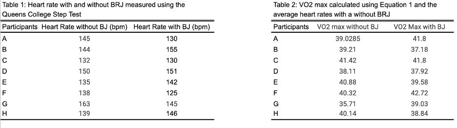
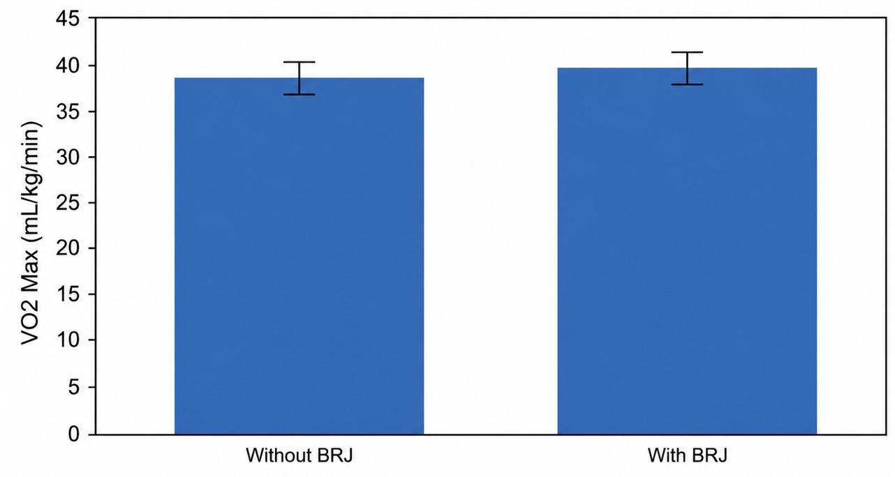
Fig. 1. Comparison of the mean VO2 max (mL/kg/min) measured without BRJ and with BRJ across all participants. Error bars represent standard error ofthe mean (SEM) indicating the precision of the estimated mean.

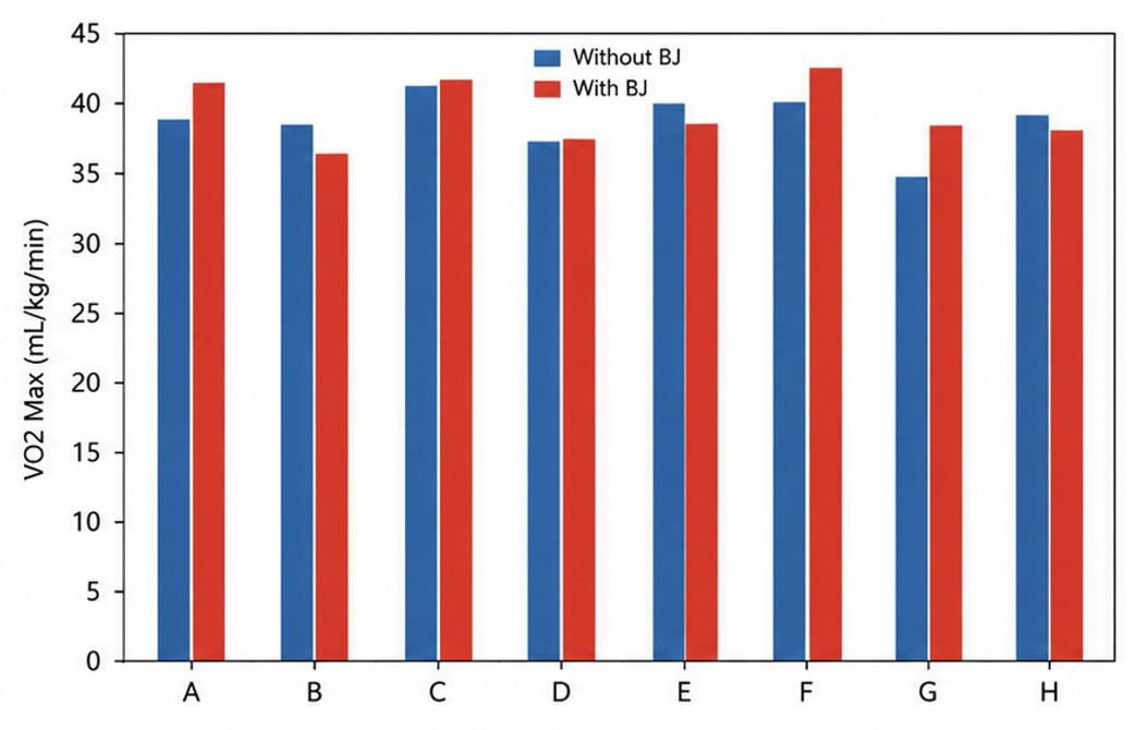
Fig. 2. Comparison of the mean VO2 max (mL/kg/min) measured without BRJ and with BRJ for each participant. Blue bars represent measurements without BRJ and red bars represent measurements with BRJ.

consume no caffeine.

On test day, the Queens College Step Test was used to determine VO2 max (Topend Sports, n.d.). Subjects were instructed to step up and down on a 15.75-inch bench to a set metronome at 88 bpm for women.The stepping consists of stepping up with your left foot, then right, and down with your left foot, then right foot. This was repeated to the metronome for three minutes. After a cycle, the participants had their pulse taken in a standing position within 5 seconds of stopping. The pulse was taken for 15 seconds, then multiplied by four to get the average bpm. Then, using equation 1, which is specific for women, VO2 max was calculated.

Equation 1: VO2 max women = 65.81 - (0.1847 x Recovery Heart Rate in BPM)

This process was repeated both with and without the BRJ. Participants were also instructed to complete a short survey after their VO2 max testing regarding questions of perceived effort.

After testing, the VO2 maxes from both tests were compared using a paired t-test for each subject to see if there was a significant change in VO2 max by comparing the test results with and without the BRJ. The results of the survey were also compared, but given that participants simply filled them out based on how they were feeling, they were not considered solid evidence to point one way or the other.

Results

Eight female runners had their VO2 max tested using the Queens College step test. Each runner repeated the test both before and after supplementing with three shots of Beet It Sport Pro-Elite BJ. The VO2 maxes were then calculated within each trial and compared. The mean VO2 max without BRJ was 39.35, and the mean VO2 with BRJ increased to 39.86 as shown on Table 1 and Figure 1. Therefore, BRJ increased the mean VO2 max by 0.51. Despite this slight increase, the results within individuals varied as presented in Figure 2. Four participants showed increased VO2 max, while the other four showed a decrease. The largest increase in VO2 was +3.32, and the largest decrease in VO2 max was −2.03. Some individuals showed notable improvement, some showed very little or even negative changes in VO2 max. Using a paired t-test, the p-value was calculated to be 0.52; therefore, the results can not be considered significant, indicating that beet juice does not have a significant effect on VO2 max in this sample.

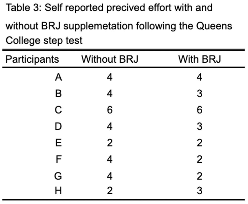
After doing the Queen’s College step test both with and without BRJ, participants reported perceived effort as shown in Table 3 and Figure 4. The mean perceived effort was 3.86 out of

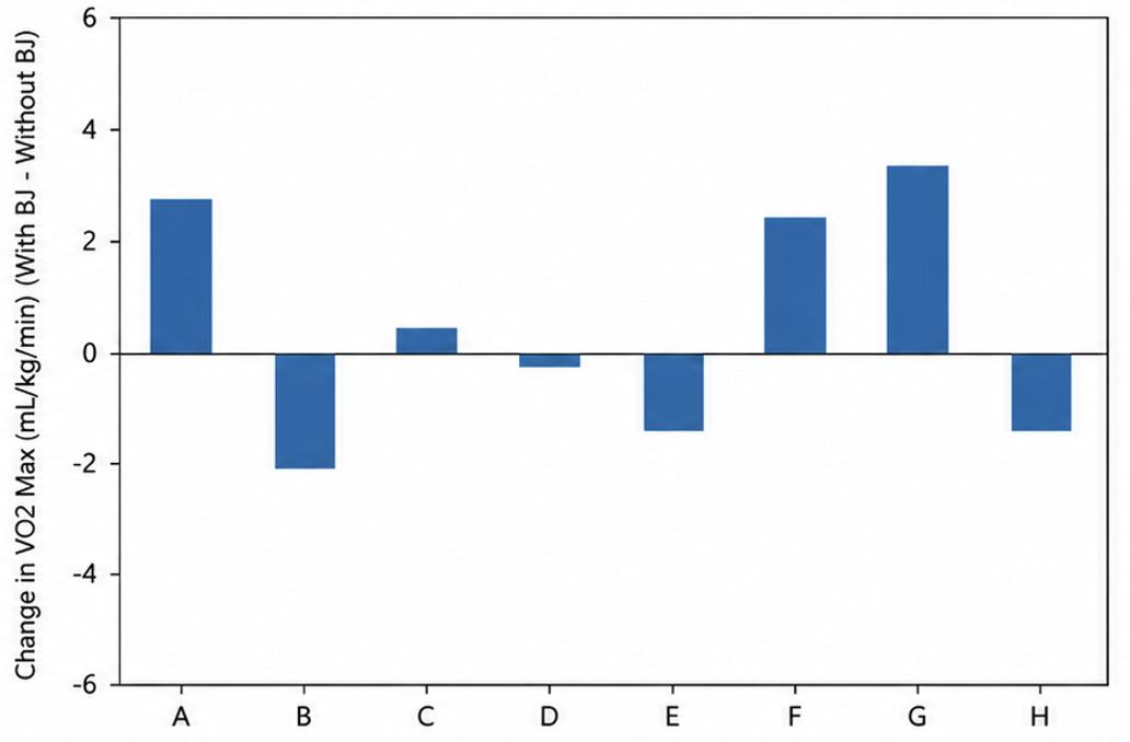
Fig. 3. Change in VO2 max (mL/kg/min) with BRJ compared to without BRJ. Positive values indicate higher VO2 max with BRJ.

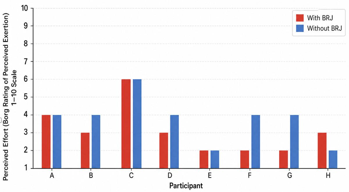
Fig. 4. Self-reported perceived effort during the Queens College step test without BRJ supplementation (blue bars) and with BRJ (red bars). Lower scores indicate the activity felt easier.

ten without BRJ and 2.57 with BRJ.This shows that within this test group, there was a reduction of 1.29 in effort when supplementing with BRJ. Individuals tended to show lower perceived effort with BRJ, but the results can not be considered statistically significant due to the small sample size. Overall, these results suggest that BRJ does not significantly affect VO2 max but may reduce perceived effort during exercise, but the results can not be considered statistically significant.

Discussion

This study investigated whether BRJ significantly improves VO2 max in endurance runners by measuring VO2 max before and after BRJ supplementation. This will help determine if BRJ has a meaningful effect on VO2 max or simply perceived exertion and overall efficacy. It is hypothesized that the BRJ will have little effect on VO2 max during endurance-based athletic performance; however, perceived effort in athletic performance may decrease, potentially due to the placebo effect. It was found that there was an increase in mean VO2 max by 0.51, but results were inconsistent; therefore, the change was not considered significant. Perceived effort had a clear decrease, with the average self-reported effort

score decreasing by 1.29 on average, showing a trend. This trend, however, was not statistically significant. So while BRJ does not appear to meaningfully improve VO2 max, it may decrease perceived effort.

The results of the VO2 testing could not be considered significant due to small, inconsistent changes across participants. Overall, the mean VO2 max did increase, but only half of the participants showed an increase in VO2 max. This could be because BRJ may not directly impact oxygen capacity and therefore endurance, as well as VO2 max. VO2 max is also difficult to change in the short term, and a longer supplementation period may be needed to provide meaningful results (Lundby et al., 2017). The most probable explanation for these findings would be that the Queens College step test may not be as precise as lab testing, such as a maximal oxygen uptake test, or a reliable enough measure of VO2 max to fully capture the subtle difference in VO2 max. But overall, the hypothesis is supported in the findings that BRJ will have little effect on VO2 max during endurance-based athletic performance. The results of the self-reported perceived effort test had a strong pattern suggesting the BRJ did lead to reduced perceived effort. Most participants reported lower perceived effort. This result could be accurate as BRJ has the ability to improve blood flow due to the nitric oxide being produced. The placebo effect also may have played a role, as participants were expecting improvement as they knew they were taking a potentially performance-enhancing supplement. So, it does appear that perceived effort in athletic performance will decrease, whether it is due to the placebo effect or increased blood flow, is unknown at this time. To address these questions, a double-blinded study would help reduce the placebo effect and blood flow, and things like oxygen delivery can be directly tested during exercise and would help to better understand what could potentially be reducing perceived effort. These results match many existing studies. Bond (2018) found that BRJ supplementation did not significantly improve VO2 max or heart rate in elite distance runners, but it did decrease reported perceived effort and exercise economy. These findings are in line with the present study and suggest that BRJ does not influence how exercise feels and may be due to only physiological effects, though the subjects used were high school track athletes, which has not been previously studied. These results are also supported by findings from Boorsma (2014), who reported that BRJ supplementation did not improve the performance of elite 1500-meter runners. He believed this was because the athlete’s physiological systems were maximally adapted, so the placebo would have no effect. In race walkers, Burke (2021) came to a similar conclusion that BRJ does not significantly impact the psychological aspect of performance. As there are conflicting opinions on whether BRJ does impact perceived effort, Lee J Wyle demonstrated how the nitrate in BRJ increases nitric oxide, which improves blood flow and oxygen (Wylie, 2013). This may not increase VO2 max significantly, but it could create a reduced effort during exercise. Overall, many studies are in disagreement on whether VO2 max is increased and perceived effort is reduced following BRJ supplementation.

There were many limitations to this study that potentially impacted the results. Sleep, diet, hydration, and muscle fatigue were not factors that were considered, but they can affect both VO2 max and perceived effort. It is also notable that the first

round of testing was done after runners were doing their own workouts, most likely easy running, while the second round of testing was done two days after a workout. This could potentially have impacted VO2 max, as after a hard workout, VO2 max drops; it will eventually recover and increase, but this varies person to person (Maughan, 2013). Perceived effort can potentially be affected by a hard workout, as a runner’s legs will most likely be most fatigued two days after the workout. Because of this fatigue, it is possible that the change in VO2 max and perceived effort appear less significant than they may be in reality.The sample size was also small, and all women were included, which limits generalizability and statistical significance. The tests used to measure VO2 max and perceived effort also had potential flaws, with the VO2 max measurement likely not as accurate due to difficulties recording heart rates and the fact that it is very difficult to measure true VO2 max without lab-based metabolic testing. Perceived effort scores were most likely heavily affected by placebo, as scores were self-reported, but it is hard to tell, as no placebo control group was able to be used.

For future research, a larger and more diverse sample is suggested. A placebo-controlled design would limit the potential effects that the placebo may have on perceived effort. As for VO2 max testing, lab testing will give more accurate results. Blood nitrate levels and time to exhaustion may also give better insight into the effect of the BRJ. It might be interesting to test using a longer supplementation period or different levels of athletes, elite vs recreational athletes.

Overall, BRJ did not significantly improve VO2 max during endurance-based athletic performance. It may also have reduced perceived effort, though the results were also not significant, and the performance benefits may be psychological due to the placebo effect.

Works Cited

Bond, V., Thompson, C., Wylie, L. J., Fulford, J., Vanhatalo, A., & Jones, A. M. (2018). The effects of beetroot juice supplementation on exercise economy, rating of perceived exertion, and running mechanics in elite distance runners: A double-blinded, randomized study. PLoS ONE, 13(7), e0200517. https://doi.org/10.1371/journal.pone.0200517

Boorsma, R., Whitfield, J., & Spriet, L. L. (2014). Beetroot juice supplementation does not improve performance of elite 1500-m runners. Applied Physiology, Nutrition, and Metabolism, 39(11), 1334–1340. https://doi.org/10.1139/ apnm-2014-0286

Burke, L. M., Hall, R., Heikura, I. A., Ross, M. L., Tee, N., Kent, G. L., Whitfield, J., Forbes, S. F., Sharma, A. P., Jones, A. M., Peeling, P., Blackwell, J. R., Mujika, I., Mackay, K., Kozior, M., Vallance, B., & McKay, A. K. A. (2021). Neither beetroot juice supplementation nor increased carbohydrate oxidation enhance economy of prolonged exercise in elite race walkers. Nutrients, 13(8), 2767. https://doi.org/10.3390/nu13082767

Lundby, C., Montero, D., & Joyner, M. (2017). Biology of VO2 max: looking under the physiology lamp. Acta Physiologica, 220(2), 218–228. https://doi.org/10.1111/apha.12827

Maughan, R. J. (2013). Nutritional ergogenic aids and exercise performance. In J. A. Barroso & T. M. Rodriguez (Eds.), Sports nutrition: ergogenic aids and supplements (pp. 95–120).

Nova Science Publishers. https://www.novapublishers. com/wp-content/uploads/2019/06/978-1-61209-334-5_ ch5.pdf

Topend Sports. (n.d.). Queen’s College step test. Topend Sports. https://www.topendsports.com/testing/tests/step-queens. htm

Wylie, L. J., Kelly, J., Bailey, S. J., Blackwell, J. R., Skiba, P. F., Winyard, P. G., Jeukendrup, A. E., Vanhatalo, A., & Jones, A. M. (2013). Beetroot juice and exercise: Pharmacodynamic and dose-response relationships. Journal of Applied Physiology, 115(3), 325–336. https://doi.org/10.1152/japplphysiol.00372.2013

J. Chapados

RESEARCH & DISCOVERY

The Effects of Estrogen on Female Runners

Katie Chapados

Abstract

Many female athletes (especially distance runners) struggle with health problems due to running, whether it be injury, missing essential hormones due to overtraining, or (most commonly) missing periods. As a female runner, there are additional challenges of hormones naturally changing due to the menstrual cycle, which can result in fatigue, soreness, and injury. Since estrogen is lowest during the follicular phase, the athletes’ races during this phase were compared to races during other phases of the period to see if the estrogen levels affected performance. Overall, distance runners showed a significant decline in performance during their follicular phase, leading to the conclusion that estrogen might be a key hormone for running. This could be tested more rigorously in future studies that control for external factors such as sleep and food intake to ensure that estrogen levels are the only factor affecting performance.

Introduction

Many female athletes, especially endurance runners, often experience amenorrhea or bone density issues. These problems can be caused by underfueling and overexertion, which lead to the brain slowing down its signaling (Sims, 2013).When the brain lacks sufficient energy, it reduces hormone production, resulting in irregular or absent menstrual cycles (Ackerman et al., 2020).

The main hormone that affects the menstrual cycle is estrogen. Estrogen is essential for the development and maintenance of the female reproductive organs, such as the uterus, ovaries, and vagina (Baar, 2019). Short-term symptoms of reduced estrogen levels in vital organs such as the ovaries include loss of the menstrual period or spotting (Sims, 2013). More severe long-term effects can include permanent damage to the ovaries, leading to infertility or cancer.

Estrogen also plays a role in female sex characteristics such as breast development, body hair distribution, and bone density (Sims, 2013). For runners in particular, healthy bone density is essential. Running is a high-impact sport that puts significant stress on tendons and bones. An athlete with low bone density is at a higher risk of developing stress fractures or breaks (Collado-Boira et al. 2021). Estrogen contributes to bone density by promoting bone formation and inhibiting bone reabsorption (Ackerman et al., 2020). It binds to bone-building cells and stimulates activity to increase bone cell formation. In addition, estrogen protects bones from osteoclasts (bone-destroying cells; Collado-Boira, E. et al. 2021). Typically, women who have gone through menopause naturally have lower levels of estrogen, leading to frailer bones (Chidi-Ogbolu et al., 2019).

Estrogen has also been shown to affect the cardiovascular system. It helps reduce stress and plaque buildup in the arteries and activates protective pathways for heart cells (Elliott-Sale et al., 2020). Perhaps the most significant benefit for runners is the impact of estrogen on cholesterol levels. Estrogen maintains a healthy lipid profile by supporting beneficial HDL cholesterol, which removes excess lipids (Khosla, S. et al., 2012). When

estrogen levels drop, LDL cholesterol (bad cholesterol) increases, and the body’s lipid balance worsens (Williams et al. T, 2015). Women naturally experience symptoms of mood changes, digestive issues, and, likely the most detrimental to athletes, fatigue. Estrogen levels are the leading cause of these negative side effects, as they can increase by 10-100 fold during the menstrual cycle. These are all linked to the menstrual cycle and typically occur monthly (Hammes et al., 2019; Baar, K, 2019).

Estrogen is clearly essential for female health, especially for athletes. The question is how much estrogen levels affect athletic performance, specifically in female runners. It is important to understand the impact estrogen levels have on the female body so that we can prevent and account for these issues. This study examines the short-term effects of estrogen levels on female athletes. By tracking the menstrual cycle, we can determine that when a female is in the early follicular phase, she has the lowest estrogen levels (Carmichael, 2021). According to the information above, females should perform worse in races during the follicular phase due to lower estrogen levels.

Methods

For this experiment, six female athletes were recruited from my Indoor Track team, all of whom had received parental consent. Participants were in high school and competed in running events ranging from the 55-meter dash to the 2-mile run. All participants tracked their menstrual cycles using the Health app on their iPhones.This data was used to identify periods of menstruation and to calculate the early follicular phase, during which estrogen levels are lowest. The team competed in weekly meets, and participants

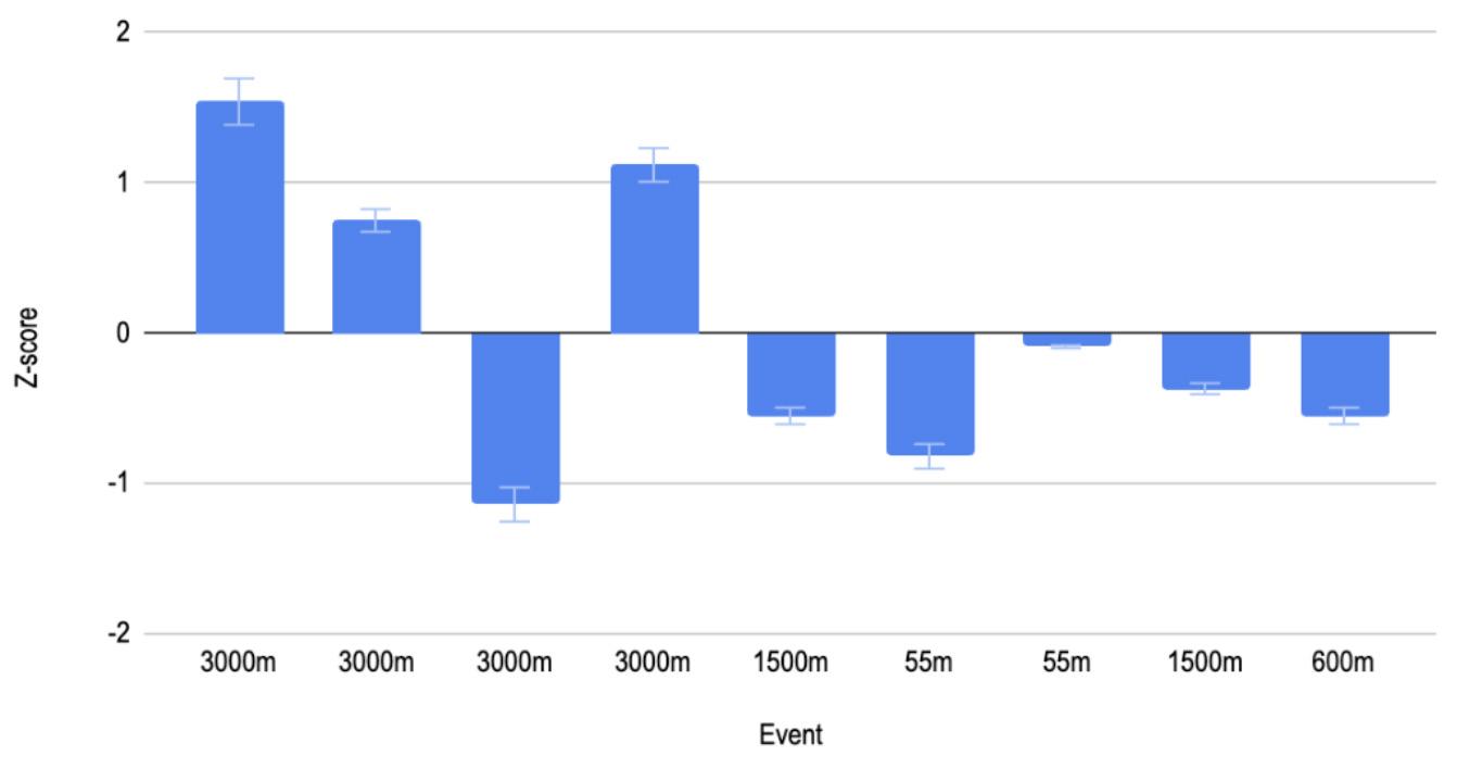
Fig. 1. Average Z - score during the lowest point of nine athletes’ estrogen production (events 3000m - 55m) over the course of the indoor track season.

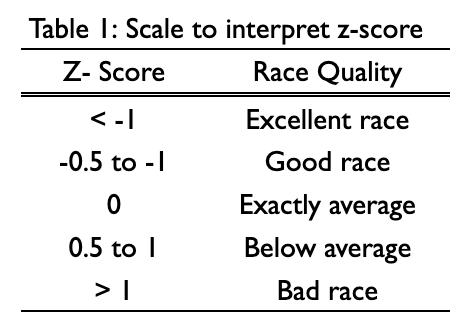
ran the same or a similar event each week. I used a mile split running conversion calculator to convert long-distance event time into the normal event the participant ran to ensure consistency in performance comparisons (MileSplit, 2026). Event times were recorded and organized into a data table that included menstrual phase and race time for each participant during each meet. By comparing race performance across different menstrual phases, I analyzed which phase was associated with optimal performance and assessed the impact of estrogen levels on athletic output. The experiment lasted the duration of the Indoor Track season, which was 14 weeks. I calculated each race’s z-score by subtracting the mean of the data from that week’s time and then dividing it by the data’s standard deviation. If the z-score was negative, the race was faster than average, and if it was positive, the race was slower than average. Using this method, I labeled each race as good or bad by following a scale that I made. Then I took the dates of each person’s menstrual cycle and compared them with each person’s performance on meet days. I made graphs labeling each race with its z-score, whether it was considered a bad or good race, and whether the athlete was in the menstruating phase. The athletes naturally expect to peak at the end of the season, so during the three to four weeks in which the athletes tapered at the end of the season, I only considered a race labeled Very Good to count as a good performance. This is why using the z-score method allows for the overall trend of performance improvement while enabling comparison across menstrual phases.

Out of the six athletes, there were a total of nine times they raced during times when their estrogen was at its lowest levels (first five days of period). Using these nine times, I made a bar graph with the athletes’ events and comparative z-scores.

Results

To analyze my performance, I first subtract the value I was testing from the athlete’s mean race time, then divide by the standard deviation to see how many standard deviations the athlete landed from their mean. A negative result indicates the race was faster than the athlete’s average time, while a positive result shows the athlete finished slower than their average time. (Table 1)

The graphs show low correlation overall between low estrogen in the follicular phase and negative performance in track events. When separating the runners into the categories

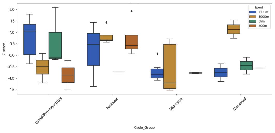
Fig. 2. All z-scores for the events athletes raced during different phases of the menstrual cycle

of distance runners (3000m), middle distance runners (1500m600m), and sprinters (55m), there was a correlation (Figure 1). For distance runners, the z -scores when they raced during the first five days of their period tended to be higher, the highest being +1.12. Three out of the four distance-categorized races were positive, showing bad races. The average z-score for distance runners racing during their periods was +0.5675, which is positive, meaning that distance runners, on average, were probably affected by estrogen levels. The middle distance runners had a majority of average races during their peak of low estrogen, the worst performance having a z-score of -0.37, and the best had a z-score of -0.55. The average z-score for middle-distance runners was -0.49, which is scaled as a slightly good race. The sprinters had a trend of good performances with an average z-score of - 0.685, which is classified as a good race. Overall, there is a suggested effect of low estrogen on distance runners and little to no effect on middle-distance runners and sprinters.

Discussion

The goal of this study was to determine whether female athletes perform worse during their follicular phase, as this is when their bodies produce the lowest levels of estrogen. This hypothesis is primarily supported for distance runners, as the average z-score for this group was +0.5675. A positive z-score indicates that performances during the follicular phase were, on average, worse than those during other phases of the menstrual cycle. Conversely, when those same runners ran races that coincided with the other phases of the menstrual cycle, z-scores were significantly reduced. Low estrogen can increase soreness, lead to faster fatigue, and make your body feel weaker. When estrogen levels are low, the body is forced to rely on carbohydrates for quick energy, meaning fuel depletion happens faster, resulting

K. Chapados

in energy crashes. VO2 max can also decrease with low estrogen, leading to higher cardiovascular strain (Williams et al. T, 2015). As distance runners rely mainly on endurance, these symptoms would have the largest effect on them.

Although there appears to be a correlation between “bad races” and the follicular phase, many other factors can influence a runner’s performance, such as diet, sleep, and training. Studies like Amir Khcharem et al.’s (2025) experiment show that even one night of sleep can lead to decreased endurance performance and effects on hematological and lipid profiles. Regarding diet, studies like Brewer & Patton’s (year) have shown that an increase in carbohydrates for endurance runners can increase performance. Additionally, the study included a limited number of athletes, which reduces the reliability of the data. In the future, it would be beneficial to focus specifically on distance runners and conduct a longer study with a larger sample size. It would also be valuable to directly measure estrogen levels to confirm whether estrogen is the factor affecting performance.

If female athletes have a better understanding of their menstrual cycles and how these cycles affect performance, they may be able to adjust their training and competition strategies accordingly, potentially improving their outcomes. Nutritional needs may also vary across different phases of the menstrual cycle, and diets containing appropriate nutrients for each phase are recommended. In more extreme cases, consistently low estrogen levels may hinder peak performance. In such situations, athletes should consider investigating the underlying causes of reduced estrogen levels. Awareness of estrogen levels is important for overall health, and especially for athletes, as it may help reduce the risk of injury. Future research on the role of estrogen will ideally contribute to greater education and awareness regarding women’s health and safety in athletics.

Works Cited

Ackerman, K. E., Singhal, V., Slattery, M., Eddy, K. T., Bouxsein, M. L., Lee, H., Klibanski, A., & Misra, M. (2020). Effects of Estrogen Replacement on Bone Geometry and Microarchitecture in Adolescent and Young Adult Oligoamenorrheic Athletes: A Randomized Trial. Journal of Bone and Mineral Research, 35(2), 248–260. https://doi.org/10.1002/ jbmr.3887

Baar, K. (2019). Effect of Estrogen on Musculoskeletal Performance and Injury Risk. Frontiers in Physiology, 9, 421933. https://doi.org/10.3389/fphys.2018.01834

Brewer, J., C.Williams, A Patton. (1988). “The Influence of High Carbohydrate Diets on Endurance Running Performance.” European Journal of Applied Physiology and Occupational Physiology, vol. 57, no. 6, 1988, pp. 698–706. https://doi. org/10.1007/BF01075991.

Carmichael, M. A. (2021). The Impact of Menstrual Cycle Phase on Athletes’ Performance: A Narrative Review. Sports Medicine – Open, 7(1), 1–15. https://doi.org/10.1186/ s40798-021-00344-3

Chidi-Ogbolu, N., & Baar, K. (2019). Effect of Estrogen on Musculoskeletal Performance and Injury Risk. Frontiers in Physiology, 10, Article 1834. https://doi.org/10.3389/ fphys.2019.01834

Collado-Boira, E., Jose Enrique Iranz- Cortez. (2021). Influence

The Effects of Estrogen on Female Runners of Female Sex Hormones on Ultra-Running. International Journal of Environmental Research and Public Health, 18(19), Article 10162. https://doi.org/10.3390/ ijerph181910162

Elliott-Sale, K. J. , Kelly L McNulty , Paul Ansdell, Stuart Goodall, Kirsty M Hicks, Kevin Thomas Paul A Swinton Eimear Dolan (2020). The Effects of Oral Contraceptives on Exercise Performance. Sports Medicine, 50(4), 673–690. https://www.ncbi.nlm.nih.gov/pmc/articles/PMC7497464/ Hammes, S. R., & Levin, E. R. (2019). Impact of Estrogens in Males and Androgens in Females. The Journal of Clinical Investigation, 129(5), 1818–1826. https://doi.org/10.1172/ JCI125755

Khcharem, A., Masmoudi, L., Sahnoun, Z., & Sahli, S. (2025). One night of sleep deprivation decreases endurance performance and affects hematological and lipid profiles in young recreational runners. Biological Rhythm Research, 56(3), 158–168. https://doi.org/10.1080/09291016.2024.2 442872

Khosla, S., Oursler, M. J., & Monroe, D. G. (2012). Estrogen and the Skeleton. Trends in Endocrinology & Metabolism, 23(11), 576–581.https://pmc.ncbi.nlm.nih.gov/articles/ PMC3424385/

MileSplitUSA, FloSports.Inc (2026). MileSplit Conversion Calculator. MileSplit.com https://www.milesplit.com/calc?time=3%3A56.5&event=1000m

Sims, M. (2013). Effects of Transdermal Estrogen on Body Composition in Adolescent Female Athletes (Doctoral dissertation, Boston University). https://open.bu.edu/server/api/ core/bitstreams/fab7addf-6022-49ec-ac3c-2d8bb0991f75/ content

Williams, T., Walz, E., Lane, A. R., Pebole, M., & Hackney, A. C. (2015). The Effect of Estrogen on Muscle Damage Biomarkers Following Prolonged Aerobic Exercise in Eumenorrheic Women. Biology of Sport, 32(3), 193–198. PDF / full-text: https://www.termedia.pl/The-effect-of-estrogen-on-muscle-damage-biomarkers-following-prolonged-aerobic-exercise-in-eumenorrheic-women,78,25740,1,1.html

RESEARCH & DISCOVERY

The Study of the Necessity of Supplements in Teenagers Diets

Olivia Fowler

Abstract

This study explores the effect of supplements in teenagers’ diets. The changes that teenagers and adolescence have during puberty leads to a higher nutritional need. Higher nutritional needs and environments that teenagers grow up in often leads to a use of supplements. Supplements (which are products that have a high level of a certain nutrient) are unlike food or drugs and are not heavily regulated by the US Food and Drug Administration, which leads to fears about the unstudied adverse effects that supplements could have on teenagers. Studies have shown that supplements are in fact not needed for teenagers if they are meeting dietary guidelines through their diet.

In this study, I used six teenagers that all took some form of a supplement and examined their diet for a day. I used a calorie tracking app called Cronometer to break down the specific nutrient levels that each subject got in their daily diet. I then compared the difference in supplement inclusion to diet for all six subjects and used a paired t-test to determine whether or not the supplement increase was significant. My results indicated that the increase in nutrient intake with supplements was not significant and therefore my hypothesis that supplements were not needed in teenagers diets was not supported.

Introduction

Teenagers and young adults experience many changes in growth, along with higher needs for different nutrients. Nutrient needs of adolescence compared to adults are relatively higher, which leads to many adolescents facing challenges in meeting their dietary needs (Parnell et al., 2016). The environments in which teenagers live can also contribute to the health challenges they might face. With childhood obesity rising in the United States, there is also a rise in diets that do not meet the required nutrition intake for teenagers (Bell et al., 2004). A “healthy diet” is one that meets a certain level of various nutrients that are essential for a good quality of life and healthy longevity. These nutrients include macromolecules, such as carbohydrates, lipids, proteins and nucleic acids, along with micromolecules such as vitamins and minerals (Wierzejska, 2021). One of the ways that many Americans meet their dietary requirements is with supplements.

Supplements are products that have high levels of a certain nutrient and are digested in addition to a regular diet. Supplements are not like conventional foods and are often a pill, or another form that can be taken orally. For example, magnesium, fiber, iron, collagen are all usually sold in pill form, while melatonin and multivitamins are often seen in gummy form. Powder supplements like creatine also exist, and even caffeine is considered a supplement, depending on its source (Rawson et al., 2018). Supplements, unlike food or drugs, do not need to be approved by the US Food and Drug Administration (FDA) before production or being put on the market (Ronis et al., 2017), which means that supplements could be advertising false or misleading health claims.

Due to the many different forms and low restriction on supplements, there has been a rise in supplement use among young adults. While there are studies on supplement use in teenagers, there is not an exact percentage of how many teenagers take supplements. However, studies show that about 50% of adults in the United States take some form of supplements (Wierzejska, 2021). Many studies also show that young adult athletes are one of the main consumers of supplements (Garthe & Maughan, 2018;

Parnell et al., 2016). Since athletes experience more intensive training for their sport, they tend to increase their calorie intake and prioritize the nutrients that are in their diets. There has also been an increasing trend of health influencers online using and sponsoring supplements (Garthe & Maughan, 2018).

The increased usage globally has led to concerns about the benefits and possible adverse effects of supplements. Due to the fact that supplements are not as heavily regulated as drugs, there are not as many studies on the possible side effects that an excess of nutrients that supplements provide could have on one’s body. While many supplements sold are generally regarded as safe, studies show that they are unnecessary with a balanced diet (Ronis et al., 2017). However, many teenagers, especially athletes, include supplements in their diet. The increased usage of supplements in teenagers’ diets led me to my study question: Are supplements necessary in a teenager’s diet?

I hypothesize that if a healthy teenager is meeting their dietary requirements, then the usage of supplements in their diet is not beneficial for them to maintain a healthy lifestyle. Due to the widespread use of supplements and the low amount of restriction

by the US government on them, it is important to understand the adverse effects that come with supplements. For this study, I intend to gain a better understanding of the prevalence and necessity of supplements in teenagers’ lives, as well as provide information on how supplements that are used by teenagers are contributing to their diets. I intend to do so by tracking different teenagers’ (both athletes and non-athletes) diets for a week to determine if the supplements that they take are truly supplementing nutritional gaps. Also, create a survey about the students at Allendale Columbia School use of supplements. My goal for this study is to help provide information on how much contribution supplements have in young adults’ lives, as well as keep those who are being tested informed on what they are putting in their body.

Methods

For my experiment, I conducted an experiment that tracked the diets of six individuals for a day using the Cronometer App. These individuals volunteered and signed forms of consent. This app tracks the calories consumed and the macronutrients and micronutrients that are part of the subjects’ diets. The subjects logged their daily meals and other food consumed by taking a photo and the app broke down the calories and the different nutrients that were consumed (Cronometer, 2026). To ensure variation in the type of teenagers that I tracked, I had five females and included one male subject as well. All of my subjects had some form of supplements that they took daily, this allowed me to analyze the necessity of supplements in their diets.

For comparison, participants’ daily nutrient and caloric intake was compared to the recommended amount of nutrients that the specific individual should be getting in their diet. The comparison that I used was the recommended amount of nutrients that is set by the National Institute of Health (NIH) (National Institute of Health). Then, I compared the specific micro/macro nutrient that the subjects consumed to the supplements they were taking. If they were consuming more than one supplement, then I included multiple different comparisons of the nutrients they were getting in their diet to the additional supplements. For this complex data, I analyzed each subject’s nutrient intake to the supplement inclusion separately. Then, I used a bar graph to do a direct comparison to the specific nutrient(s) that the subject was

getting with the supplement to the amount that was in their diet and used. Then, I took the disproportion of the specific nutrient in the diet to supplement inclusion for all six subjects. For my statistical analysis, I used a paired t-test with a significance level of 0.05 to see if the difference between the two groups was significant.

Results

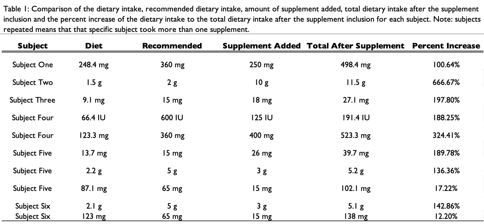
The main trend seen here is that supplementation increased nutrient intake for all subjects. All subjects except for subject four met or exceeded the recommended dietary intake with supplement inclusion. Table one shows that the amount of which nutrient intake increased varied by subject.There was a large range of increased intake from 12.2% to 666.67%. Another trend seen in Table One is that the largest increase in nutrient intake occurred when the original intake levels were low and the supplement inclusion was larger than the recommended dietary intake, as seen in Subject Two who had a nutrient increase of 666.67%. On the other hand, subjects who already had higher baseline intakes generally had the lowest percentage difference like one of the nutrients for subject five and one of the nutrients for subject six, which had a difference of 17.22% and 12.2%, respectively.

A large trend seen in Figure One is that the nutrient intake level for all subjects variated substantially. While some subjects exceeded the recommended daily value by a large percentage, some subjects only increased their intake levels a little bit and therefore did not have as large of a gap between intake levels after supplementation and the recommended intake. This trend likely contributed to the large standard deviation that was seen in the paired t-test. A final trend seen is in Figure Two with the paired t-test showing that the difference in intake level before and after supplementation was not statistically significant.

Discussion

In my experiment, I hypothesized that if a healthy teenager is meeting their dietary requirements, then the usage of supplements in their diet is not beneficial for them to maintain a healthy lifestyle. My results did not result in a p-value lower than 0.05 and therefore they were not statistically significant and my hypothesis was not supported. Figure Two showed that the pair t-test concluded that

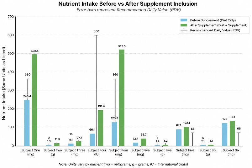
Fig. 2. Comparison of nutrient intake before and after supplement inclusion. Blue bars represent the nutrient intake from diet alone, while green bars represent the total nutrient intake including supplements. Error bars indicate the recommended daily intake value for each specific nutrient. Note: subjects repeated means that that specific subject took more than one supplement and nutrient units vary by the specific nutrient and includes milligrams (mg), grams (g) and International Units (IU).

made a significant difference. This means that the subjects did not have enough nutrients that they were getting through their diet that the supplements were not needed. Although my results were not significant, there is still a strong trend of the subjects exceeding recommended intake levels with supplementation by a large percentage. Although this trend cannot be fully supported because of the sources of error in the experiment.

One of the biggest sources of error was the difference in nutrient levels for each specific supplement. The different levels of supplements for each subject created a large variation. This variation causes the standard deviation to be quite larger which affected my result of the test. Another source of error was the small number of subjects that I had. The six subjects and nine supplements that were used in the paired t-test also created a wide variability. These two errors reduced the statistical significance of my data and therefore affected my results.

Another limitation was the accuracy of the caloric input. For many of my subjects, the total caloric intake was low compared to the NIH recommended total caloric intake. Also, the Cronometer App cannot be 100% accurate when breaking down the nutrient levels for each individual food that is consumed. Finally, the differences between each of my subjects could have been a limitation. Each subject varied by sex, weight and activity level and thus had different nutritional needs than others. Although this was partially taken into account, there was still a small gap between what the NIH recommended nutritional values are and what each specific subject actually needs.

Although the data was not significant, it provides some scientific evidence that there is a strong trend of gaining nutritional needs through diet rather than supplementation. While there is some knowledge on this topic, it is still worth continuing experiments and expanding knowledge on all supplements, especially because of the lack of knowledge on the adverse effects and low regulation

there is not a large enough increase in nutrient intake before and after the inclusion of supplements to say that the supplements be more beneficial to have a more accurate source of data with a larger sample size. Also, focusing on a specific supplement, rather than all supplements would allow the results to be more accurate and specific to that certain supplement. More research would create safer food environments not only for teenagers, but for everyone.

Works Cited

Bell A., Dorsch K. D., Mccreary D. R., Hovey R (2004). A look at nutritional supplement use in adolescents. Journal of Adolescent Health, 34 (6), 508-516 https://www.jahonline. org/article/S1054-139X(03)00348-3/fulltext

Cronometer. (2026). Cronometer (4.48.2) [Mobile application]. https://cronometer.com

Garthe I & Maughan R. J. (2018) Athletes and Supplements: Prevalence and Perspectives International Journal of Sport Nutrition and Exercise Metabolism 28 (2), 126-138. https://journals.humankinetics.com/view/journals/ijsnem/28/2/ article-p126.xml?content=fulltext

National Institutes of Health, Office of Dietary Supplements (2026). Dietary Reference Intakes (DRIs) and Nutrient Recommendations for Adolescents (14–18 years). https://ods.od.nih.gov/healthinformation/nutrientrecommendations.aspx?utm_source=chatgpt.com

Parnell A. J., Weines K. P., Erdman K. A. (2016). Dietary Intakes and Supplement Use in Pre-Adolescent and Adolescent Canadian Athletes. Nutrients, 8 (9), 526-539 https://www. mdpi.com/2072-6643/8/9/526

Rawson E. S., Miles M. P. & Larson-Meyer E. (2018) Dietary Supplements for Health, Adaptation, and Recovery in Athletes. International Journal of Sport Nutrition and Exercise

Metabolism 28 (2), 188-199 https://journals.humankinetics.com/view/journals/ijsnem/28/2/article-p188.xml?content=fulltext

Ronis M J.J., Pedersen K. B., Watt J. (2017). Adverse Effects of Nutraceuticals and Dietary Supplements. Annual Review of Pharmacology and Toxicology, 58, 583-601 https:// www.annualreviews.org/content/journals/10.1146/annurev-pharmtox-010617-052844

Wierzejska RE. (2021) Dietary Supplements-For Whom? The Current State of Knowledge about the Health Effects of Selected Supplement Use. Int J Environ Res Public Health. 24;18 (17), 8897.doi https://pmc.ncbi.nlm.nih.gov/articles/ PMC8431076/

RESEARCH & DISCOVERY

The Effects of Energy Drink Consumption on Athletic Performance

Lauren Garsin

Abstract

Athletes often consume energy drinks thinking they will help them focus, increase energy levels, and improve performance. The purpose of this study was to determine if consuming an energy drink prior to exercise had an effect on reaction time, grip strength, and cardiovascular endurance of female high school athletes. Athletes completed testing sessions with and without an energy drink. Consumption of energy drinks did not lead to significant improvements in reaction time, grip strength, resting heart rate, or blood pressure. There were, however, important differences in cardiovascular responses during exercise, particularly in the heart rate and blood pressure changes following the three-minute step test. These findings suggest that energy drinks may alter the cardiovascular response to exercise, but they do not consistently improve short-term physical or cognitive performance. More research with a larger sample size is needed to better understand the effects of energy drinks on athletic performance and health.

Introduction

Energy drink consumption has increased significantly over the past 20 years with the creation of new drinks and successful marketing strategies (Heckman et al., 2010). Energy drink companies claim their product will improve athletic performance by increasing focus and energy levels, but there is no consistent evidence to prove their claims are accurate (Jacobson et al., 2018). These companies often utilize social media to effectively advertise their product to their target audience: young adults, especially athletes (Erdmann et al., 2021). While these advertisements appeal to individuals, the actual health effects are much more complicated than these companies reveal.

Some individuals reported that they experienced side effects immediately after consuming energy drinks, such as tachycardia, or increased heart rate, dehydration, temporary high blood pressure, restlessness, and difficulty breathing (Jacobson et al., 2018). These beverages often contain stimulants such as taurine, an amino acid naturally produced by the human body that contains sulfur, and caffeine, a central nervous system stimulant. Taurine is included in energy drinks to increase energy levels, improve focus, and enhance muscle efficiency (Seidel et al., 2019). Caffeine blocks adenosine, a chemical in the brain that causes individuals to feel exhausted. As a result, it reduces fatigue, increases energy levels, and boosts focus (Smith, 2002). The quantities of these substances are sometimes unlisted because the FDA does not require manufacturers to disclose them, so consumers do not know how much they are putting into their bodies. Athletes seeking to boost their mental and physical performance often drink energy drinks, but they do not know what is in them because companies do not disclose the ingredients. It is concerning that individuals do not have access to this information, given the harmful side effects (Erdmann et al., 2021).

Energy drinks may appear beneficial immediately after consumption, but they can lead to health problems over time. Studies have found that excessive energy drink usage causes damage to the heart and brain, essential organs in the human body.

The high levels of caffeine in energy drinks cause increased heart rate and blood pressure, which can lead to heart attacks. Energy drinks affect the brain by overactivating the nervous system, possibly causing anxiety, headaches, and, in extreme cases, seizures or strokes (Lazzari et al., 2023). Consuming energy drinks can also cause insomnia, obesity, diabetes, and damage to the liver over time (Alsunni, 2015).

The purpose of this experiment was to determine whether consuming energy drinks prior to athletic training improved athletic performance among athletes of different skill levels and sports. Young athletes are increasingly using energy drinks due to their ergogenic effects (Duchan et al., 2010). In a study of 707 young athletes, it was found that 69% consumed energy drinks, and 17% of them consumed energy drinks weekly (Nowak & Jasionowski, 2016). It is important for athletes and individuals who choose to consume energy drinks to know how the ingredients in these beverages affect their bodies and to fully understand the advantages and risks of consuming these beverages in order to make informed decisions about their health. In this study, one type of energy drink was tested for its effects on endurance, strength, and reaction time. I hypothesized that consuming the energy drink would improve reaction time while having no significant effect on strength and endurance.

Methods

I recruited ten high school athletes to participate in my study. To ensure a diverse sample, I aimed to include athletes from different sports. Upon testing, the participants were required to provide informed consent and complete a survey. The survey collected data on the participant’s athletic background and history with energy drink consumption. Each participant completed two testing sessions. Before testing, participants were instructed not to consume caffeine for 24 hours, engage in high-intensity exercise for 12 hours, or eat within two hours of testing to ensure accurate results.

In the first session, the participant’s reaction time was tested by completing a test three times using computer software developed by Human Benchmark (Human Benchmark, n.d.). Strength was then measured using a handgrip dynamometer (TIPRE digital hand-held grip strength dynamometer; model HS01). To obtain consistent measurements, the participant gripped the device’s handle, exerted maximum force for three seconds, and rested for two minutes between attempts. The participant completed two trials using their dominant hand. The participant then rested three minutes before completing the next test. To test cardiovascular endurance, the participant completed the three-minute step test. Prior to completing the test, the participant’s heart rate and blood pressure were taken using a digital blood pressure monitor. Then, to complete the test, the participant stepped up and down a 12inch platform for three minutes following a metronome set at

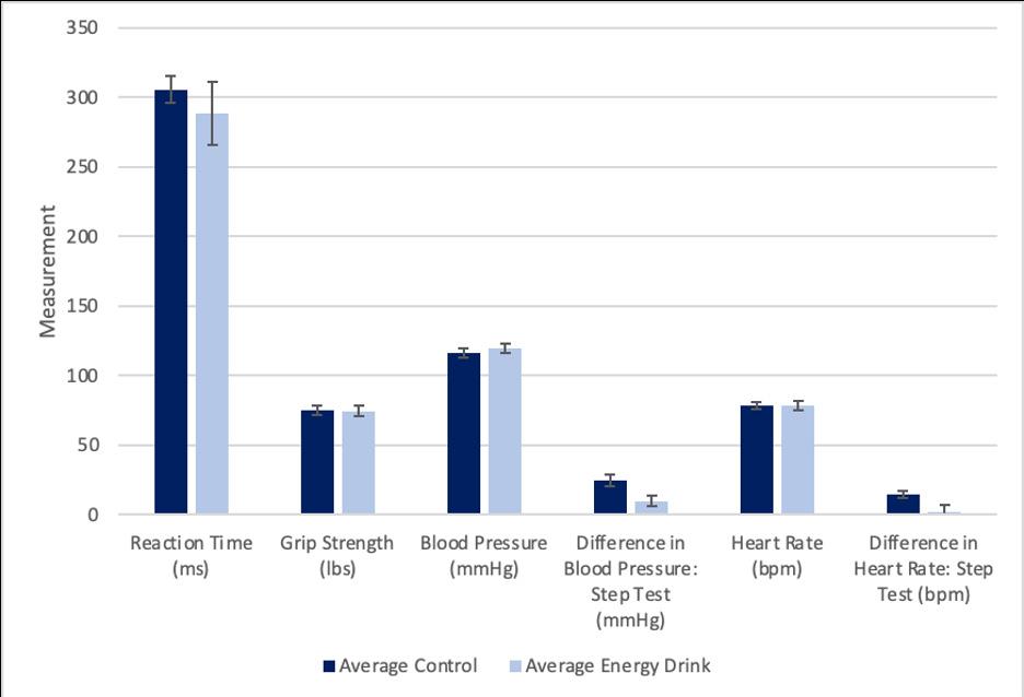
Fig. 1. Tthe average reaction time, grip strength, blood pressure, and heart rate for the control and energy drink groups. Error bars represent the standard error.

88 bpm (Physio-Pedia, n.d.). Following the three-minute test, the participant immediately sat down, and their heart rate and blood pressure were taken again. This concluded the testing for the first session.

In the following session, at least 48 hours later, the participant consumed a 12-fl-oz Alani Nu energy drink within a ten-minute period. The participant then rested for 30 minutes to allow the caffeine and taurine, key ingredients in the beverage, to reach their peak levels in the bloodstream so I could measure the actual effect of the energy drink (Jacobson et al., 2018). Following the 30-minute time period, the participant’s heart rate and blood pressure were taken using a digital blood pressure monitor. The testing for reaction time, strength, and cardiovascular endurance was then repeated.

I compared the results from both sessions using paired t-tests to determine the effect of energy drink consumption on reaction time, strength, and cardiovascular endurance. Faster reaction times, higher average grip strength, and lower post-exercise heart rate and blood pressure values following energy drink consumption were interpreted as evidence of improved performance.

Results

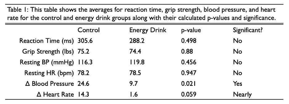
A statistical analysis was conducted to determine the differences between the energy drink and control groups in reaction time, grip strength, heart rate, and blood pressure. The average values for each variable were calculated for both groups. The average reaction time for the control group was 305.6 ms, whereas the energy drink group averaged 288.2 ms. Grip strength was similar between the two groups, with averages of 75.2 lbs for the control group and 74.4 lbs for the energy drink group. Resting blood pressure was slightly higher in the energy drink group (119.8 mmHg) compared to the control group (116.3 mmHg). Resting heart rate was also very similar, averaging 78.2 bpm in the control group and 78.5 bpm in the energy drink group. During the three-minute step test, the control group showed an average blood pressure difference of 24.6 mmHg, compared to 9.7 mmHg for the energy drink group. The average heart rate difference during the three-minute step test was 14.3 bpm for the control group and 1.6 bpm for the energy drink group.

Paired t-test showed no significant differences in reaction time (p = 0.498), grip strength (p = 0.88), resting heart rate (p = 0.947), or resting blood pressure (p = 0.456) between the control and energy drink groups. However, a statistically significant difference was found in the change in blood pressure (p = 0.021).The change in heart rate was close to being statistically significant with a

p-value of 0.059. These results are shown in Figure 1 and Table 1.

Discussion

I hypothesized that consuming an energy drink would improve reaction time while having no significant effect on strength or endurance. Although participants demonstrated slightly faster reaction times after consuming an energy drink, the difference was not statistically significant, and grip strength, resting heart rate, and resting blood pressure showed little variation between the control and energy drink groups. Therefore, the results did not support much of the original hypothesis. The most notable finding came from the three-minute step test, during which participants in the control group exhibited greater increases in both blood pressure and heart rate than those who consumed an energy drink. While the change in blood pressure was statistically significant and the change in heart rate approached statistical significance, these findings suggest that energy drinks may not improve reaction time or strength but could influence cardiovascular responses during exercise.

Despite careful procedures, several sources of error may have affected the accuracy and reliability of the results. Different caffeine tolerance levels of participants may have affected how strongly the energy drink influenced each person. Participants who consume caffeine often may have developed a higher tolerance than those who do not consume caffeine as often or at all (Alsunni, 2015). The energy drink may have less of an effect on participants who consume caffeine more frequently. If this experiment were conducted again, the participants should be grouped by how often they consume caffeine.The equipment used to measure blood pressure and heart rate also had some errors, which may have led to inaccurate measurements. Following the three-minute step test, the digital blood pressure monitor did not always record measurements immediately. For some participants, an ERROR message appeared on the monitor after the first and sometimes second attempts. As a result, it took multiple attempts to read these measurements, which could have altered the results by allowing heart rate and blood pressure to drop from their original numbers. A future experiment could solve this issue by using more accurate equipment. Another source of error could be that the sample size was too small (n = 10) to accurately measure the differences between the control group and the energy drink group. A larger sample size would allow for stronger and more reliable results by reducing the margin of error.

This study adds to existing research by showing that energy drinks may not significantly improve short-term reaction time or grip strength.These findings support previous studies, such as those conducted by Smith (2002) and Jacobson et al. (2018), which found that energy drinks do not consistently enhance physical or cognitive performance.The current study also suggests that energy drinks may affect cardiovascular responses during exercise due to significant differences in the change in blood pressure and a nearly significant difference in the change in heart

rate following physical activity. Overall, the results indicate that energy drinks do not consistently enhance mental and physical performance in athletes.

In future research, this experiment could be repeated with a larger sample size and tighter control of experimental variables to reduce the influence of individual differences. Future studies should more carefully control factors such as sleep, hydration, caffeine tolerance, and fitness level. Additional studies could focus on different brands of energy drinks or the long-term effects they have on the human body. Continued research will help clarify the benefits and risks of consuming energy drinks.

Acknowledgments

I would like to thank Mr. Godkin for teaching the Science Writing and Research course and for guiding me throughout this project. I would also like to thank Allendale Columbia School for funding my research. In addition, I am grateful to my classmates for providing valuable feedback on my work and for assisting with the peer-review process.

Works Cited

Alsunni, A. A. (2015). Energy drink consumption: Beneficial and adverse health effects. International Journal of Health Sciences (Qassim), 9(4), 468–474. https://www.ncbi.nlm. nih.gov/pmc/articles/PMC4682602/

Duchan, E., Patel, N. D., & Feucht, C. (2010). Energy drinks: A review of use and safety for athletes. The Physician and Sportsmedicine, 38(2), 171–179. https://www.tandfonline.com/doi/abs/10.3810/ psm.2010.06.1796

Erdmann, J., Wiciński, M., Wódkiewicz, E., Nowaczewska, M., Słupski, M., Otto, S. W., Kubiak, K., Huk-Wieliczuk, E., & Malinowski, B. (2021). Effects of energy drink consumption on physical performance and potential danger of inordinate usage. Nutrients, 13(8), 2506. https://www.mdpi. com/2072-6643/13/8/2506

Heckman, M. A., Sherry, K., & Gonzalez de Mejia, E. (2010). Energy drinks: An assessment of their market size, consumer demographics, ingredient profile, functionality, and regulations in the United States. Comprehensive Reviews in Food Science and Food Safety, 9(3), 303-317. https://ift.onlinelibrary.wiley.com/doi/10.1111/j.15414337.2010.00111.x

Human Benchmark. (n.d.). Reaction time test. HumanBenchmark. com. https://humanbenchmark.com/tests/reactiontime

Jacobson, B. H., Hester, G. M., Palmer, T. B., Williams, K., Pope, Z. K., Sellers, J. H., Conchola, E. C., Woolsey, C., & Estrada, C. (2018). Effect of energy drink consumption on power and velocity of selected sport performance activities. Journal of Strength and Conditioning Research, 32(6), 1613–1618. https://pubmed.ncbi.nlm.nih.gov/28723815/ Lazzari, J., Casula, C., Turillazzi, E., Frati, P., & Fineschi, V. (2023). The

Garsin The Effects of Energy Drink Consumption on

Dark Side of Energy Drinks: A Comprehensive Review of Their Impact on the Human Body. Nutrients, 15(18), 3922. https://www.mdpi.com/2072-6643/15/18/3922

Nowak, D., & Jasionowski, A. (2016). Analysis of consumption of energy drinks by a group of adolescent athletes. International Journal of Environmental Research and Public Health, 13(8), 768. https://www.mdpi.com/16604601/13/8/768

Physio-Pedia. (n.d.). Step Test. In Physio-Pedia. Retrieved January 14, 2026, from https://www.physio-pedia.com/Step_Test

Seidel, U., Huebbe, P., & Rimbach, G. (2019). Taurine: A regulator of cellular redox homeostasis and skeletal muscle function. Molecular Nutrition & Food Research, 63(16), e1800569. https://onlinelibrary.wiley.com/doi/10.1002/ mnfr.201800569

Smith, A. P. (2002). Effects of caffeine on human behavior. Food and Chemical Toxicology, 40(9), 1243–1255. https://www.sciencedirect.com/science/article/abs/pii/ S0278691502000960?via%3Dihub

RESEARCH & DISCOVERY

Evaluating the Cellular Impact of Bacopa monnieri on Yeast Proliferation

Gabriella Giambra

Abstract

This study investigated the cellular impact of Bacopa monnieri, a traditional nootropic herb, on the proliferation of Saccharomyces cerevisiae (baker’s yeast). While previous research has identified the anti-cancer and neuroprotective properties of Bacopa monnieri in mammalian models, the fundamental effects on eukaryotic cell division remain less known and explored. It was hypothesized that exposure to Bacopa monnieri would decrease the rate of cell division. Using a controlled experimental design, rehydrated yeast cultures were treated with standardized Bacopa monnieri solution and were compared with a distilled water and yeast control group.

The result supported the hypothesis, revealing a 40% reduction in cell concentration in the experimental group (48,000 cells/mL) compared to the control group (411,200 cells/mL). A two-sample t-test confirmed these findings were statistically significant (p=0.000031).

Introduction

Bacopa monnieri, more commonly known as brahmi, is a plant traditionally used in Ayurvedic medicine to support memory, focus, and overall brain health.Ayurvedic medicine is a form of medicine which originated from India and it involves the use of herbs like Bacopa monnieri in aims to support a holistic approach to health, balancing mind, body, and spirit. Bacopa monnieri’s active compounds, called bacosides, have been shown to reduce oxidative stress, decrease inflammation, and influence cellular signalling pathways (Alzheimer’s Research & Prevention Foundation, 2021).While most studies tend to focus on the neurological effects of Bacopa monnieri , more recent studies suggest that Bacopa monnieri may have effects on fundamental cellular processes, including cell growth, division, and apoptosis (Saha et al., 2020; Ghosh et al., 2020).

The cell cycle is the process by which cells grow, replicate their genetic material (DNA), and divide. Sometimes the cycle is paused at certain checkpoints to repair DNA damage or respond to environmental signals.This pause is known as cell arrest. During cell cycle arrest, a cell temporarily stops progressing through the cycle, and if the issue cannot be resolved, it may remain halted, preventing further division (Shukla et al., 2025). Studying cell arrest gives us insight into how compounds like those found in Bacopa monnieri influence the timing of and rate of cell division, which has implications for cancer research.

Previous studies in mammalian cancer cell lines have shown that Bacopa monnieri extracts and isolated compounds like Bacopaside II can reduce cell proliferation and promote apoptosis (Ghosh et al., 2021). These anticancer effects have been reported in colon, lung, breast, and oral cancer cell lines, suggesting that Bacopa monnieri’s bioactive compounds can influence key pathways involved in overall survival and cell division (Ghosh et al., 2021; Sun et al., 2025). While this research demonstrates that Bacopa monnieri can alter cell cycle regulation and induce programmed cell death in mammalian systems, most studies have focused on cancer models.As a result, its effects in other eukaryotic organisms remain less studied and explored. Yeast is widely used as a model organism for studying cell division because it grows rapidly, is

easy to manipulate experimentally, and shares highly conserved cell cycle pathways with more derived eukaryotes, making it a valuable system for investigating fundamental mechanisms of cellular regulation.

An additional motivation for this study is the growing popularity of nootropic supplements that claim to improve focus and cognitive performance. Bacopa monnieri is commonly included in these products and has been studied for its neuropharmacological effects, particularly its potential role in memory and cognitive function (Saha et al., 2020; Alzheimer’s Research & Prevention Foundation, 2021). However, whole clinical research typically uses standardized extracts at specific doses; commercial supplements can vary widely in formulation and concentration. Because of this, it is important to examine whether Bacopa monnieri produces measurable biological effects at the cellular level rather than relying solely on marketing claims. Investigating its impact on yeast cell division allows for a more controlled evaluation of its biological activity.

The purpose of this study is to determine whether Bacopa monnieri affects cell division in yeast and, if so, to characterize the nature of those effects. Previous research has shown that Bacopa monnieri extracts can influence cellular processes such as proliferation and apoptosis in certain cell models, particularly in

Giambra

cancer research (Ghosh et al., 2021). Some studies suggest that Bacopa monnieri may interfere with normal cell cycle progression, leading to reduced cell growth under specific conditions (Ghosh et al., 2021). Based on these findings, it is hypothesized that Bacopa monnieri will alter the rate of yeast cell division, potentially slowing progression through the cell cycle. Examining these effects in yeast provides a simple model to better understand Bacopa monnieri cellular impact (Mallick et al., 2015).

Methods

A dilute culture of Saccharomyces cerevisiae (baker’s yeast) was prepared so that individual cells could be clearly seen and counted. About 0.25 g of active dry yeast was rehydrated in 100 mL of warm sugar water made by dissolving 0.5g of granulated sugar and 10mL of distilled water at 30-35°C. This temperature range was selected to optimize yeast metabolic activity while avoiding thermal stress.

The Bacopa monnieri liquid concentrate was prepared prior to experimentation by dissolving 0.5 g of Bacopa monnieri powder in 30 mL of water, following the instructions provided on the product packaging. The solution was heated to 30–35°C to activate its properties before mixing with yeast.

For the experimental treatment, one mL of the yeast culture was combined with one mL of the prepared Bacopa solution in a petri dish. The control group consisted of one mL of yeast culture and 1mL of distilled water. After combining, all samples were incubated at room temperature, 20°C to 22°C for one hour to allow for cell growth. This hour of incubation allowed for the Bacopa monnieri to possibly inhibit cell growth. Each group contained ten samples: five experimental and five controls. Making a total of ten tests done throughout one test round.

Following incubation, cell viability and concentration were assessed using a hemocytometer under a microscope. For each sample, 100 µL of 0.1% methylene blue concentration was mixed with 100 µL of either the yeast-only or yeast-Bacopa solution to stain the cells. Methylene blue was utilized as a viability indicator, as non-viable cells lack the enzymes necessary to reduce the

Evaluating the Cellular Impact of Bacopa monnieri on Yeast Proliferation

dye, resulting in a blue stain (Sami et al., 1994). A micropipette (bio pipette) was used to transfer all solutions, and tips were rinsed with distilled water between samples to prevent crosscontamination. Microscope slides were cleaned with Kimwipes after each use. Cells were counted via the four outermost squares and the center square,with five replicates for both the control and experimental groups. Counting this way was done to eliminate any potential bias.

To calculate the average cell count, the number of cells in each square was recorded and then added together for each trial. That total was divided by the number of squares counted to find the average number of cells per square.

This was done for all five replicates in both the control and experimental groups. Then, the averages from each replicate were added together and divided by five to get the overall average cell count for each group.

To estimate the cell concentration, the average number of cells per square was multiplied by the hemocytometer conversion factor of 104, taking into account the volume of each square and the 1:1 dilution that occurred during staining. This allowed for an estimate of the number of cells per milliliter in each sample. To determine if the differences between the control and experimental groups were statistically significant, a two sample t-test was conducted using Microsoft Excel. A p-value of less than 0.05 was established as the threshold for significance.

Results

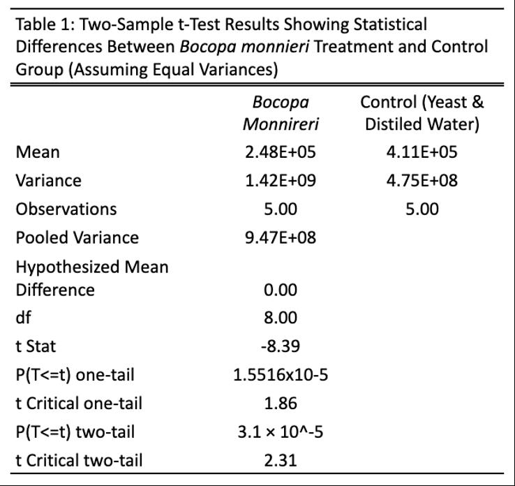
The impact of B. monnieri on yeast cell proliferation was measured by comparing cell counts between the liquid yeast cultures treated with B. monnieri and the control, which was just the untreated liquid yeast culture. In Figure 1, the cultures treated with B. monnieri resulted in a lower average cell count of approximately 248,000 alive cells per mL with a standard error of 16840.43. In comparison to the control group, which averaged approximately 411,200 living cells per mL with a standard error of 9,748.85. A two tailed t-test was used to determine if the differences in cell growth between the control and the treated culture was significant. The test produced a t-statistic of -8.387 with eight degrees of freedom and a two tailed p-value of 0.000031031. Since the p-value is significantly smaller than 0.05,

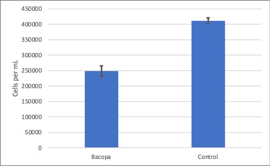
Fig. 1. Average yeast cell count for Bacopa monnieritreated and control groups. Error bars represent the standard error of the mean (SEM).

Giambra

the results indicated a statistically significant decrease in living cells for the group treated with B. monnieri

Discussion

The objective of this study was to determine if Bacopa monnieri impacts cellular division using Saccharomyces cerevisiae (Baker‘s yeast) as a model organism. It was hypothesized that the introduction of Bacopa monnieri would alter the rate of yeast cell division, specifically by slowing progression through the cell cycle. The results supported this hypothesis, the experimental group treated with Bacopa monnieri had a significant 40% reduction in cell concentration, averaging 248,000 cells/mL on average in comparison to the control group which averaged 411,200 cells/ mL. The results also showed a statistically significant p-value of 0.000031, which suggests that bioactive compounds like bacosides can possibly stop cells from dividing in similar ways to previously studied mammalian cells (Saha et al., 2020). Alternatively, it is important to look at other possible explanations for our results, the Bacopa monnieri concentration could have possibly killed the cells instead of just slowing division. It is possible the extract interfered with the general survival rather than just the cell cycle, perhaps by damaging the cell membranes or blocking the yeast’s ability to process energy. The concentration might have also changed the overall pH of the liquid, making it harder for the yeast to stay alive. Also, errors like yeast clumping and mistakes when counting with a hemocytometer could have affected the results. To address these counting errors in future trials, a digital imaging system or automated counter could be used to ensure higher accuracy. However, because the same rehydration and counting procedures were applied to both the control and experimental groups, these errors likely occurred at the same rate across all samples and likely do not account for the large 40% difference observed. Even considering these possible sources for error, this study still shows that Bacopa monnieri affects basic cell growth in simple cells. Since this study only tested a specific concentration based on the product packaging, it is unclear on how the effects may change with different dosage. Future studies should focus on identifying the specific phase of the cell cycle arrest, testing a wider range of concentrations to find the exact point in which cell growth is inhibited, and transitioning to human cells to establish a clear answer due to the fact human cells are much more complex than yeast cells. The evolution into studying human cells will allow for a more reliable understanding of Bacopa monnieri effects within the human body.

Acknowledgments

This study was funded and supported by the Allendale Columbia School. I would like to acknowledge and thank Mr. Godkin and Raylee Stearns for their unwavering support and assistance in conducting this experiment.

Works Cited

Alzheimer’s Research & Prevention Foundation. (2021). Bacopa monnieri: Cognitive vitality media update [White paper]. https://www.alzdiscovery.org/uploads/cognitive_vitality_ media/Bacopa_monnieri_UPDATE_%28supplements%29. pdf

Ghosh, S., Khanam, R., & Chowdhury, A. A. (2021). The evolving

Evaluating the Cellular Impact of Bacopa monnieri on Yeast Proliferation

roles of Bacopa monnieri as potential anti-cancer agent: A review. Nutrition and Cancer, 73(11–12), 2166–2176. https://doi.org/10.1080/01635581.2020.1831016

Saha, P. S., Sifontes-Rodríguez, S., Rodríguez-Sánchez, J. P., & Ramos-López, M. A. (2020). In vitro propagation, phytochemical and neuropharmacological profiles of Bacopa monnieri (L.) Wettst.: A review. Plants, 9(4), 411. https://doi. org/10.3390/plants9040411

Sami, M., Ikeda, M., & Yabuuchi, S. (1994). Evaluation of the alkaline methylene blue staining method for yeast activity determination. Journal of Fermentation and Bioengineering, 78(2), 212–216. https://doi.org/10.1016/0922-338X(94)90292-5

Sun, J. R., Zhao, W. M., Zhou, B. J., Qiao, H. Z., Li, J. M., Ma, S. Q., & Zhang, J. K. (2025). Anticancer potential of ethanolic Bacopa monnieri L. extract: Induction of intrinsic apoptosis in A549 lung cancer cells. Journal of Physiology and Pharmacology, 76(6), 661–671. https://doi.org/10.26402/ jpp.2025.6.04

RESEARCH & DISCOVERY

Playing it Forward: The effects of varying sports participation on the development of psychopathological symptoms in adolescents

Evie Jackson

Abstract

Although research has been conducted looking into the effects of sports participation on the development of eating disorders in adolescents, their effects on cognitive disorders is significantly under-researched.This meta study was conducted in an attempt to evaluate the correlation between participation in solo and/or team sports on the development of psychopathological symptoms in adolescents. Data on sports participation and psychopathology assessment from a 20-year period (1990-2020) were collected and assessed and individual variables (varying survey results, sex, underlying conditions) were isolated. The compiled data was then analyzed and correlation between the development of Generalized Anxiety Disorder (GAD), Major Depressive Disorder (MDD) and Attention Deficit Hyperactivity Disorder (ADHD) and certain types of sport participation could be seen. This study can inform future diagnosis and treatment plans, possibly being integrated in prevention of certain symptom developments.

Introduction

The development of many neurological psychopathologies, such as Attention Deficit Hyperactivity Disorder (ADHD), Major Depressive Disorder (MDD), and Generalized Anxiety Disorder (GAD), are strongly linked to behavior; for this reason behaviors surrounding individuals throughout their lives can influence the severity of symptoms, therefore increasing the likelihood of the development of these symptoms into worsened psychopathologies (Rutter et al., 1997). One leading example of these surrounding behaviors in children are the clubs and activities with which these individuals choose to fill their extra time. (Singh .R, 2012) Possibly the largest sector of these activities is sports. Sports, being defined as a specialized subset of structured, repetitive physical activities designed to improve fitness and performance, have already been seen to have both a positive and negative effect on the mental wellbeing of adolescents (Haff, 2010). Many studies have found this trend, such as those which have looked at the link between team sports and prevalence of depressive symptoms in young children, finding that team sports actually decrease the prevalence of these symptoms (Khan et al., 2022).

Whilst there has been a noticeable correlation between sports and the worsening of symptoms leading to the eventual development of eating disorders (ED) in psychopathology, there is a gap in research regarding the effects of experiences in sports and the development of symptoms (both in worsening and preventing) in anxiety, depressive, and intellectual disorders (Chapa et al., 2022). Unlike EDs such as Anorexia Nervosa, Bulimia Nervosa and Binge-eating Disorder; anxiety, depressive and intellectual psychopathology symptoms are present in a person from birth. However, the development and severity of these symptoms can change drastically throughout time based on external factors (American Psychiatric Association, 2013).

The minimal research that has been conducted on this subject is somewhat contradictory. Some projects focus on lowintensity sports and the positive effects of the social interaction involved in sports and how this may protect against worsening psychopathology symptoms, and work to reduce their severity. For example in a study from 2020 the Strength of Recommendation Taxonomy-grade (SORT) level was used to see the active effect of team sports on pathology in adolescents but focused solely

on low intensity club sports and so had little variation on stress levels for participants (Chang et al., 2020). However, a few other studies focus on sports and the environmental factors that could be detrimental to an individual, developing their symptoms further and increasing their severity (Bohnert & Garber, 2007).

For this reason, I wanted to utilize such studies and broader examinations of mental health and sports to see if there is any relationship between the increase or decrease of severity in psychopathology symptoms as a result of sports participation in adolescents, and determine if a relationship between participation in team versus solo sports and an increased severity of psychopathology symptoms is present (team sports being defined by sports activities in which more than one person plays as a ‘team’ against a group of people for mutually gained points and win/loss conditions).

Methods

Adolescent mental health is largely impacted by the activities and processes of an individual’s daily life. One such element that has been seen to have significant effect, is an individual’s participation

in sports activities (Kunitoki et al., 2023). While, the development of EDs has a high correlation with participation in sports activities, the effect of sports on neurodevelopmental disorders is much less researched and so the following methodology was conducted to help find a clearer understanding of how an individual’s level of adolescent sports participation affects the reduction or development of anxiety, depressive, and intellectual disorder symptoms.

Data was taken from five different sources (indicated by * in the works cited section) on the effects of team vs solo sports on mental health in adolescents (10-18 years old), excluding individuals who have been specifically diagnosed with psychopathologies, to avoid the effects of any worsening of symptoms due to natural psychopathological development. The data was then examined and compared by examining age, frequency of sports, individual vs team sports, sports intensity, as well as their results from standardized, official surveys including the Childhood Behavioural Checklist (CBCL) (whose sections can be used separately to determine more specific symptoms), Problem Solving Inventory (PSI) and Beck Depression Inventory (BDI), which were used to determine the severity of their symptoms (American Psychological Association, 2001; Hardt, 2008). Once the data had been condensed, it was formatted to tables and graphs, in order to more easily view differences within the data sets. This was examined using Standard Mean Difference, while accounting for variability with the t-tests . In an instance where the data showed little to no difference, this information could be used to show how the frequency of sporting activities in adolescence is not related to development/worsening or alleviating of psychopathology symptoms. Where significant discrepancies were identified, trends

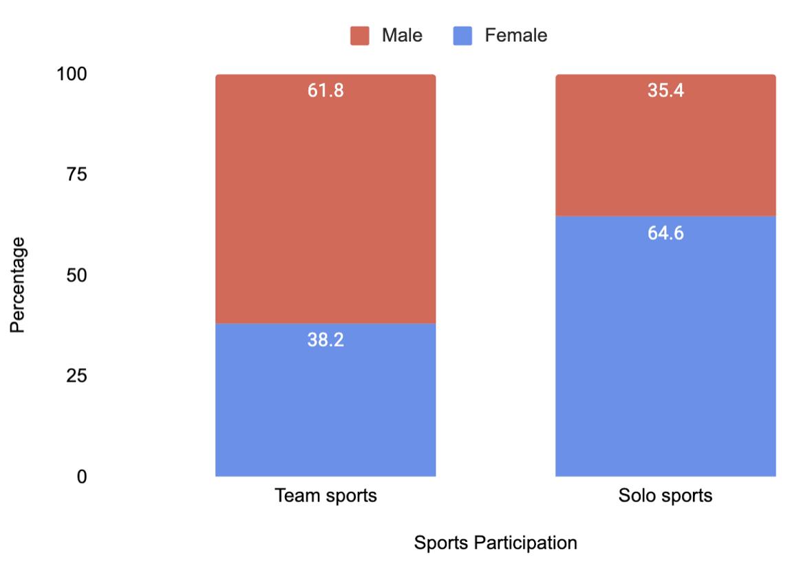
Fig. 1. Male vs Female participation in Solo and Team sports (2000-2025). Solo Sports n=3437. Team Sports n=6201

could be recognized, helping to further determine the effects of sporting activity on the adolescent’s symptom development.

Results

Data from over a period of 25 years (2000-2025) was used and analyzed. Over this 25 year period, results of standardized testing for MDD, GAD and ADHD were collected case by case and analyzed, using the Beck Depression Inventory (BDI) and Problem Solving Inventory (PSI), Childhood Behaviour Checklist (CBCL) scores, and CBCL Anxiety-depression scores respectively. These results were analyzed to find significant differences in individuals who participated in solo sports, and those who participated in team sports.

Figure 1 demonstrates the percentage of male and female participants across the 25 year period. Solo sports saw a 64.4% to 35.4% split between female and male participants, whereas team sports saw an opposite proportion with 38.2% female and 61.8% male participation.

Figure 1. Male vs Female participation in Solo and Team sports (2000-2025). Solo Sports n=3437. Team Sports n=6201

Depression symptoms were measured using two tests, taken by all selected participants, the BDI and PSI, both of which are self-survey style questionnaires recognised as one of the official factors on which MDD can be diagnosed (Khan et al., 2022). Tested scores in those who participated in team sports fell within a range indicating a lack of abnormalities on both the PSI and BDI scales, with an average score of 12.02 on the BDI and 97.65 on the PSI (Scores considered normal BDI: 0-13, PSI: 90-100). However, solo sports participants were found to have significantly different scores with both tests indicating increased depressive symptoms (Score average BDI: 17.01, PSI: 78.11; Table 1;t-test, p<0.001).

Additionally, the CBCL was used with specific focus on ADHD indication, as this test is one of the most widely used methods of symptom indication.The CBCL is a self-survey questionnaire, used most often in ADHD and GAD diagnosis. It was found that both participants who were involved in team sports and solo sports had no indication of increased worsening of ADHD symptoms in correlation to their sports (t-test; p > 0.05). On average, scores fell below 65, which is the lower bound on which ADHD diagnosis can be based.

Symptoms of generalized anxiety were also measured using CBCL scores, this time focusing on anxiety-depression score indication. In this instance, solo sports were found to have slightly lower than average scores, although not significantly different enough from the general population, averaging at 53.6 (Average score indicating an absence of abnormalities is 55. A score greater than 65 is the accepted lower bound of a complete absence of anxiety-depressive symptoms). However, when looking at those who participated in team sports it can be seen that there is a

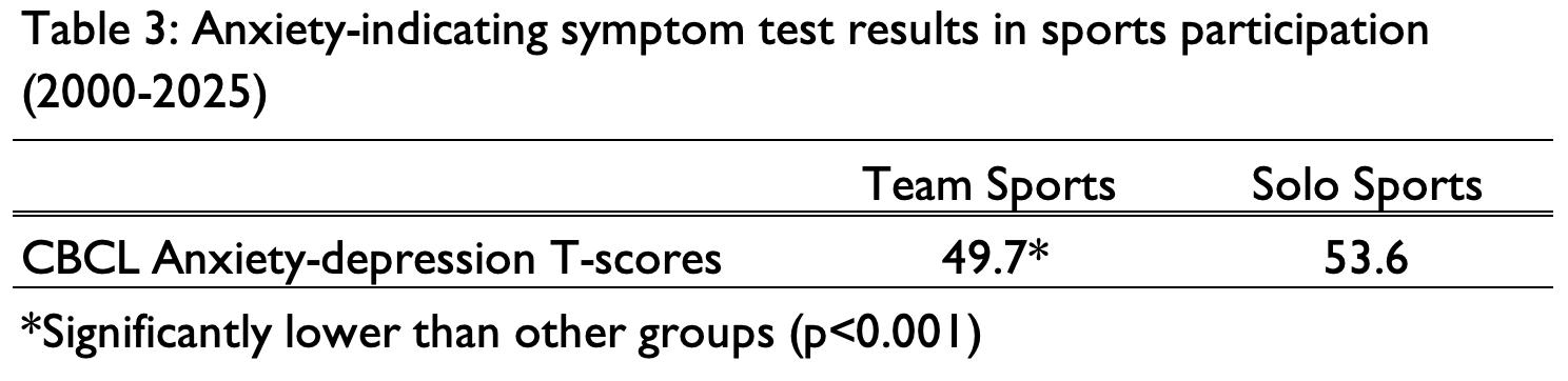
significant drop in scores. Adolescent athletes who participated in team sports had anxiety-depression scores averaging 49.7, indicating an increase of worsening symptoms (t-test: p<0.001).

Discussion

The aim of this study was to understand if there is a significant correlation between adolescents’ participation in solo versus team sports on their development of anxiety, learning, and emotional psychopathological disorder symptoms. Data was collected from over a twenty-five year period and compiled into graphs and tables in order to better view correlations between specific variables.

As is visible through the graphs and calculated statistical significance, there is correlation between the prevention of Generalized Anxiety Disorder symptoms and team sports, possibly due to increased sense of belonging and support from team mates, fostering a more anxiety-free space. There is also a visible connection between solo sports participation and the worsening of depressive symptoms (increasing risk of MDD). It is suspected, then, that although solo sports require high levels of determination, self-confidence, and decreased anxiety, this reliance on purely yourself can increase the let down when failure occurs, as the individual is not losing as a team; in their eyes the loss is solely through fault of their own.

It was made sure that all participants had no previous indication of psychopathology, and ensured that no participant was on a psychopathology-specific drug. However, other health factors, including unrelated medications and underlying conditions, could have influenced results of this data, altering certain neuroprocessings and increasing/decreasing symptoms more severely than those without. Similarly, participation in other activities could also have an effect on results. Many students chose to participate in multiple activities so it is likely that a large selection of people included in this study also had influences from participation in other extracurricular activities.

This study would highly benefit from continued research into more specific variables, as well as other psychopathologies (as this study specifically focuses on only three major psychopathologies). These studies would likely also gain off stricter guidelines surrounding co-variables, either by looking into correlation as a result of said variables or restricting participation. Also, it may be valuable to research the effectiveness of implementing/removing certain types of sports activities as one part of treatment for already diagnosed psychopathologies.

Therefore, this data shows us that there is correlation

between participation in sports and psychopathological symptoms and this can help with the diagnosis and treatment plan of future patients. Information from this study could be integrated into treatment plans itself due to correlations such as those found between GAD and team sports. However, this does not show that sports participation is able to prevent development or worsening of psychopathology completely, but more that it is a factor that could be brought into account when looking at decreasing symptoms.

Works Cited

American Psychiatric Association. (2013). DSM-5 TM. https:// dn790004.ca.archive.org/0/items/APA-DSM-5/DSM5.pdf

American Psychological Association. (2001). Child Behavior Checklist (CBCL). https://www.apa.org/depression-guideline/child-behavior-checklist.pdf

*Bohnert, A. M., & Garber, J. (2007). Prospective Relations Between Organized Activity Participation and Psychopathology During Adolescence. Journal of Abnormal Child Psychology, 35(6), 1021–1033. https://doi.org/10.1007/ s10802-007-9152-1

*Chang, C. J., Putukian, M., Aerni, G., Diamond, A. B., Hong, E. S., Ingram, Y. M… (2020). Mental Health Issues and Psychological Factors in Athletes. Clinical Journal of Sport Medicine, 30(2), e61–e87. https://doi.org/10.1097/ jsm.0000000000000817

*Chapa, D. A. N., Johnson, S. N., Richson, B. N., Bjorlie, K., Won, Y. Q., Nelson, S. V… (2022). Eating-disorder psychopathology in female athletes and non-athletes: A meta-analysis. International Journal of Eating Disorders, 55(7). https:// doi.org/10.1002/eat.23748

*Haff, G. G. (2010). Sport Science. Strength and Conditioning Journal, 32(2), 33–45. https://doi.org/10.1519/ ssc.0b013e3181d59c74

*Hardt, J. (2008). The symptom checklist-27-plus (SCL-27-plus): a modern conceptualization of a traditional screening instrument. GMS Psycho-Social Medicine, 5, Doc08. https:// pmc.ncbi.nlm.nih.gov/articles/PMC2736518/

Khan, A., Ahmed, K. R., Hidajat, T., Kolbe-Alexander, T., Edwards, E. J. (2022). Examining the Association Between Sports Participation and Mental Health of Adolescents. International Journal of Environmental Research and Public Health. Mdpi.com. https://doi.org/10.3390/ijerph192417078

Kunitoki, K., Hughes, D., Elyounssi, S., Hopkinson, C. E., Bazer, O. M., Eryilmaz, H…(2023). Youth Team Sports Participation Associates With Reduced Dimensional Psychopathology Through Interaction With Biological Risk Factors. Biological Psychiatry Global Open Science, 3(4), 875–883. https:// doi.org/10.1016/j.bpsgos.2023.02.001

Rutter, M., Dunn, J., Plomin, R., Siminoff, E., Pickils, A., Maughan, B… (1997). Integrating nature and nurture: Implications of person–environment correlations and interactions

for developmental psychopathology. Development and Psychopathology, 9(2), 335–364. https://doi.org/10.1017/ s0954579497002083

Singh, R. (2012). Positive and Negative Impact of Sports on Youth. Academia.edu, 3(4).

RESEARCH & DISCOVERY

Cost-Benefit Analysis of Uranium vs. Thorium

Jude Maguire-Mueller

Abstract

This paper aims to compare the cost-benefit analysis of thorium and uranium as nuclear fuels.We see how a thorium molten salt reactor compares to a uranium light water reactor through different stages of building, such as the initial capital cost, the fuel cycle cost (cost to maintain), and the combined Levelized Cost of Electricity. We also go deeper into the problems with switching to thorium before the reactors are even considered, talking about supply chains, mining costs, and the overall head start that uranium has over thorium in all those areas. After the comparisons, we go into a deep dive into the economic impacts of not only those calculations, but also investor preferences, environmental impacts of nuclear waste, and socioeconomic impacts.

Introduction

The 21st-century global energy landscape is defined by a double objective: meeting rising electricity demand and transitioning towards a sustainable, low-carbon energy system. With these parameters, a low-carbon option immediately presents itself: that of nuclear fuel. It offers a potential source of reliable, baseload power with very limited greenhouse gas emissions in operation. Since nuclear reactors were first proposed in theory, and even now, the primary way they’ve been powered is with uranium fuel. Although other elements have been present in the fuel, including, in rare cases, thorium, uranium has been the primary element, with any additional elements functioning alongside uranium; for example, Light Water Reactors (LWRs) use a uranium dioxide (UO2) fuel (Kasten, 1970). The economic, safety protocols, and fuel cycle logistics are well-established, having been defined over decades of commercial operations and regulatory experience. A substantial body of literature thus exists concerning cost-benefit analysis of uranium-fuelled systems, considering everything from front-end fuel costs and operational efficiency to back-end waste management and decommissioning (Kim et al., 2010; Emblemsvåg, 2024; Kasten,1970).

In conjunction, the discussion of advanced nuclear technologies has increasingly identified the potential of thorium as an alternative nuclear fuel. Advocates for Thorium, especially in concepts like Thorium-based Molten Salt Reactors (TMSRs), put forward many significant advantages: higher relative abundance of Thorium than uranium in the Earth’s crust, improved inherent safety due to passive safety systems and lower operating pressures, reduced production of long-lived radioactive waste, and inherent proliferation resistance since the fuel cycle does not produce weapons-grade plutonium (Emblemsvåg, 2024). Theoretical benefits, as described in several contemporary reviews (Çakar, 2022), position Thorium as one of the most interesting candidates for the next generation of nuclear energy.

Although this sounds promising, we immediately encounter critical practical challenges that come in the form of a deep lack of the same informational treatment that uranium has received, including a cost-benefit analysis to prove the previously claimed advantages. The possibility of the benefits that Thorium fuel cycles present is frequently discussed; however, there is a lack of relevant, peer-reviewed studies that convert these features into a comprehensive economic evaluation, benchmarking them directly against the established uranium fuel cycle. Any new energy technology must demonstrate its economic viability if it is to be commercialised and adopted on a large scale. Without a clear understanding of full lifecycle cost–encompassing research and

development, fuel fabrication, reactor construction, operation, maintenance, waste management, and decommissioning–the promise of Thorium remains in the realm of speculation. This literature gap constitutes a significant barrier to informed policy decisions, investment choices, and strategic energy planning.

Adding to this challenge is the fact that some of the basic environmental and impact assessments for nuclear energy are also quite old. For example, one of the most accessible reference documents, the “review of the Environmental Impact of Nuclear Energy” from the 1977 IAEA conference in Salzburg, has historical value concerning the uranium fuel cycle (Blanco et al., 1977).

Although this paper’s findings can give us a proper baseline to work off of, the author couldn’t possibly predict how things like inflation or discount rates could change over the almost 50 years since the paper was published.The author also couldn’t have considered the technological advancements. Because of these inaccuracies, we aren’t able to accurately rely on this paper when making modern-day comparisons between modern-day nuclear fuels. Therefore, in order to conduct an accurate cost-benefit analysis of a Thorium-based nuclear fuel, we will have to use other, more relevant works. Although we can still take information from Blanco et al. (1977), we will have to take the information while being skeptical.

A study by Kim et al. (2010) can provide just that; we can use this to give us a cost-benefit analysis of a type of uranium fuel.

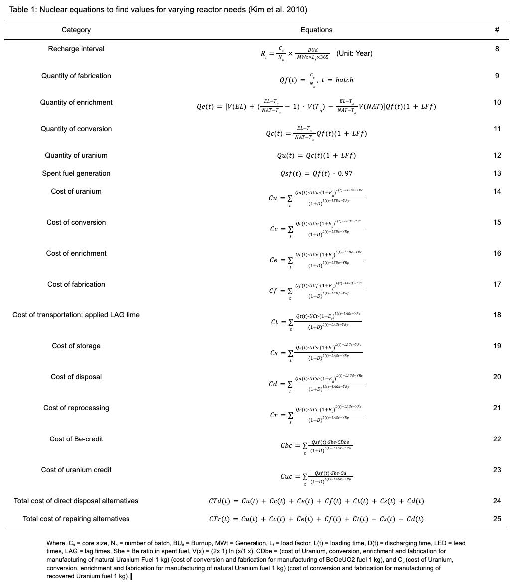
Maguire-Mueller

Their study goes into extreme detail about the Berillium-Uranium fuel, and they identify the major cost drivers (parts of the fuel that would take up the most of the fuel cost) and the benefit drivers (parts of the fuel that take up the least of the fuel cost). Kim et al. take all of the information and plug it into some calculations, shown in Table 1, and come to a “break-even” point. We can use this study to find a foundation to step on when conducting our cost-benefit analysis, using the study to find parameters and a framework for the comparison between our uranium and thorium. By adapting the tested approach from the BeO-UO2 study and understanding it with both historical and contemporary data related to nuclear fuel cycles, this study attempts to provide a simple yet extensive economic outlook on a subject that has plagued the minds of nuclear physicists and investors alike.We will look beyond theoretical benefits and place a provable cost-benefit analysis of both uranium and Thorium nuclear fuel, and in doing this, could prove a potential needed turn in the path of nuclear power away from uranium and towards thorium.

Methods

This study uses a comparative Cost-Benefit Analysis (CBA) framework to assess the economic viability of the Thorium fuel cycle against that of the established Uranium fuel cycle. The methodology has adapted a tested CBA model from existing literature on advanced Uranium-based fuels (Kim et al., 2010) and applied its logical structure to Thorium, given that there is no commercially deployed Thorium economy to which this work can be directly compared on an empirical basis.

Understanding the benefit analysis of Uranium

This analysis leans on the foundational methodology developed by Kim et al. (2010) in their Cost-Benefit Analysis of BeO-UO2 fuel. The authors systematically quantify the fuel’s life cycle cost based on the Nuclear Facilities Control Committee (NFCC), from raw material acquisition to final waste disposal. The core of their model is the set of engineering-economic equations that calculate the quantity and cost of materials and services required to generate a unit of electricity. The benefit of using uranium in general is the fact that it is a fissile element, meaning that uranium can hold a charge by itself. And thorium is a fertile element, meaning it is unable to hold a charge on its own and needs a “kick-start” by a fissile “seed” like U-235 or plutonium, which transmutes into Uranium-233, which then could sustain a charge. Uranium-233 is used for advanced nuclear cycles, primarily when thorium is used in a Light Water Reactor (LWR). But because of Uranium’s long use, it has made the transfer to thorium a massive investment when we start to think about building the new reactor types and trying to establish this commercial fuel cycle from scratch. Table 1 can help us calculate the cost of different parts of our Cost-Benefit Analysis.

Converting the Cost-Benefit Analysis of Uranium to that of Thorium

The Kim et al. (2010) document fits our objective perfectly because the fuel that they talk about (BeO-UO2) has more of a burn-up and therefore less waste; however, it is more expensive upfront. When looking at a possible comparison to Thorium, we run into a roadblock because there are no Thorium reactors in operation (IAEA, 2005). However, we can use the similarities

Cost-Benefit Analysis of Uranium vs. Thorium

that Thorium has with the fuel that Kim et al. use in their paper. Thorium fuel itself might be cheaper, but building a new type of reactor (a Molten Salt Reactor) would be expensive, and there is no physical proof that a Thorium reactor would work and be comparable to Uranium (Kasten, 1970).

To further create similarities to the Uranium Cost-Benefit Analysis, we must identify the cost drivers and the benefit drivers of using Thorium fuel.

Cost Drivers for Thorium

Looking at our Uranium fuel, we can see that it includes Beryllium(Be) in the fuel; we won’t need beryllium anywhere in our Thorium fuel; therefore, we can take that out of the equation and insert an initial higher cost of building a Thorium reactor. Also included as a cost driver would be the complex chemical processing (reprocessing, using equation 21, Cr, from Table 1.

Benefit drivers for Thorium

The benefit of high burn-up is the same. As stated in the cost driver, we can replace the “Be credit” with a “Thorium credit,” reflecting that Thorium itself is more abundant and cheaper than Uranium. The main benefit is a significant decrease in long-term disposal costs. After all, the half-life of thorium is about 3 times that of uranium, which matters because the shorter half-life means more radiation is produced.

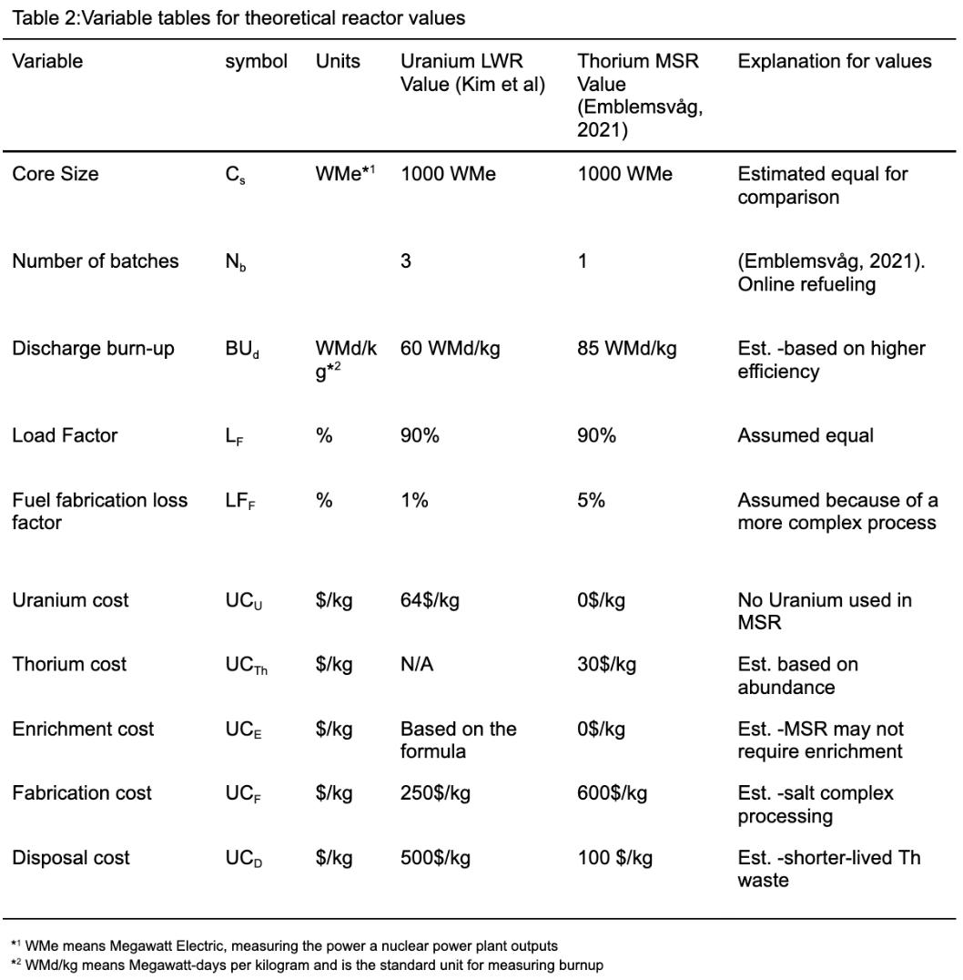
Theoretical Measurements for the Needed Variables

For our calculation, we need proper variable values for Uranium and Thorium (our core size, batch number, burn-up, etc.). Since a full-scale Thorium reactor does not exist, we need to use the variables from Kim et al.’s paper and estimate how Thorium is expected to perform.

Now that we have our estimated values for our Molten Salt Reactor, we can insert these values into our equations from Table 1 and compare and contrast the cost of each step in our Uranium

and Thorium reactors. Of course, the variables for our Molten Salt Reactor are highly estimated based on information from Kim et al. (2010) and Emblemsvåg (2021). So if replicated in real life, we can’t solely rely on these numbers and calculations.

Data Collection

Using the variables from Table 2 and the equations from Table 1, we can calculate the total fuel cycle cost of our Uranium and Thorium reactors, and to keep the comparison as similar as possible, we will use the “direct disposal” Eq. 24 as our final equation.

According to the International Atomic Energy Agency, the values of enrichment and storage/disposal, being the main cost drivers of our calculated cost, are up to par with their studies (IAEA, 2005)

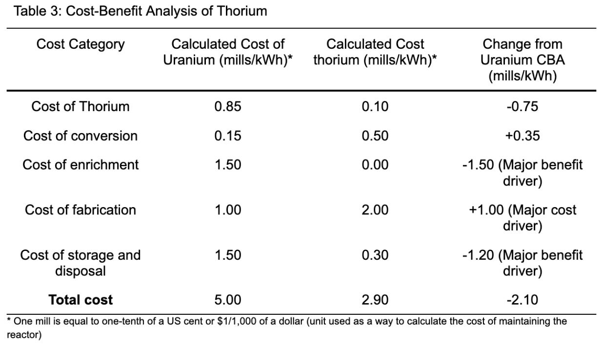
Using these tables, we can see that there are trade-offs to both of the reactors. The Uranium LWR reactor takes less money to build; however, it has a higher Mills/kWh (5.00 vs 2.90). On the other hand, the Thorium MSR is more expensive to build upfront,

but as discussed before, it has a lower Mills/kWh.

Results

In this study, we’ve focused on two different fuel types: a widely accepted fuel, uranium fuel that is used for a Light Water Reactor, and a theoretical thorium fuel, used for a Molten Salt Reactor. The results are presented in three parts: 1) The cost of the fuel cycle over its lifetime, 2) The capital cost of the initial building of the reactor, and 3) a final combined analysis using the Levelized Cost of Energy (LCOE).

Fuel Cycle Cost Comparison

Using our equations and the theoretical values that we’ve defined in our method section, the total lifetime fuel cycle cost of each reactor type was calculated. The total cost contains everything from fuel procurement to enrichment costs and final waste disposal.

Table 5 shows the calculations for our fuel, including enrichment, fabrication, storage, and disposal. It includes trade-offs, where our fuel is less appealing when compared to our uranium fuel, and our benefits, where our fuel is more appealing when compared to our uranium fuel. All of these calculations come from a thorium fuel used in a Molten Salt Reactor, and a Light Water Reactor using our BeO-UO2 fuel. When we compare these two fuel types, we see

that the thorium fuel cost has an advantage over the uranium fuel, mostly because of thorium’s enrichment cost being substantially lower than that of uranium, as well as the abundance being 90% cheaper than uranium, with better waste management, storage, transportation, and disposal. All of these factors add up to the fact that, in theory, the use of a thorium reactor is economically better than that of a uranium reactor.

Capital Construction Cost Comparison

Although we’ve established that the cost of maintaining either of the reactors favors our theoretical thorium MSR reactor, we must also consider the initial capital cost of building the reactors themselves. Initially, this cost will be the biggest benefit or cost driver, and can deter people from spending that amount of money to build the more expensive reactor if there is a cheaper alternative. To keep the comparison as fair as possible, we will continue using the cost breakdown for a 1000 MWe power plant.

Building this first-of-a-kind thorium MSR would be more expensive than a normal uranium reactor because of the new materials that would be incorporated into the reactor. A new kind of specialized salt-handling system, most importantly, a lack of an established supply chain) For these specialized ingredients. The most significant of those is a source of thorium. Although there is around 4 times the amount of thorium as uranium, there isn’t a readily available established market for thorium.

Like in all of these calculations, when talking about the MSR, these calculations are completely theoretical, and in this specific scenario, the calculations are very optimistic, and the ~10% increase in capital costs could be just a fraction of how much more an MSR costs to build when compared to an LWR.

Integrated Cost Analysis: Levelized Cost of Energy (LCOE)

The two systems of power production can be compared using a Levelized Cost of Energy, which combines the investment and the fuel cycle cost and produces a single unit for our cost of electricity: US Dollars per megawatt hour (USD/MWh; U.S. Department of Energy).

In the final analysis, using our new unit, we will be using the scenario of a reactor over 60 years with a 4.5% discount rate or return on investment, which means that the higher the discount rate is, the more risk there is in investing in that project*. Additionally, a half-time, so 30-year, refurbishment was included in both of the costs; this way, most of the factors can be accounted for in the estimations.

*It is important to mention that the discount rate fluctuates from year to year and country to country, not specifically from nuclear reactor to nuclear reactor

Although the initial capital cost of the Thorium reactor was

higher than that of the uranium reactor, the MSR in both scenarios was favored over the LWR in our LCOE ratings in USD/MWh. The reason for this ~15% advantage that thorium gets is most likely due to the almost half fuel cycle cost compared to uranium (see table 1). Because thorium has a lower LCOE, that shows that even with the initially higher capital cost, in the long run, or at least over 60 years, we can see that thorium has the upper hand over uranium.

We use the two scenarios, the U.S. and South Korea, to simulate a cheaper and more expensive scenario. The U.S. has a discount rate of ~4.5%, while South Korea has a discount rate of ~3%, although not too different from the U.S. rate, as shown in the table, it makes a pretty big difference. The discount rate is used mainly to estimate the LCOE in different parts of the world, but it can also be used to plan for the future. If a country has a certain discount rate, then they could theorize the cost if they were to plan to get to a different discount rate.

Discussion

When looking at our results, we can see that a simple costbenefit analysis can spiral into strong, quantitative, and qualitative evidence that supports our objective of looking for a better alternative to uranium-based nuclear fuel. Thorium-based Molten Salt Reactors (MSR) are more economically viable, and more importantly, a safer alternative to our comparison, a Uraniumbased Light Water Reactor, when we look at a source of nuclear energy. The results show that substantial long-term operational savings are achieved through a theory-based fuel; these operational savings not only basically cancel out the higher initial capital cost of building the reactor, but are also directly responsible for the lower levelized cost of electricity (LCOE).

The results show two initial observations: our accepted Uranium-based Light Water Reactor shows a lower initial capital cost, but loses in the comparison of both our fuel cycle costs and our Levelized Cost of Energy (LCOE). The burden of our operating costs comes from our constant need for enrichment, which is over three times the cost compared to thorium, and the large waste management cost, including storage, transportation, and disposal. This cost alone showed a 5:1 ratio of Uranium to Thorium (Table 6). Thorium is the opposite of Uranium; it has a higher initial capital cost, but a lower fuel cycle cost and a lower LCOE. The higher capital cost can be derived from the lack of any existing monopolies on Thorium fuel supply chains, the creation of which would require a huge investment of between $4-5 billion (Norman et al. 2023).

As it stands, according to all of our calculations,Thorium wins in two out of the three cost-benefit analyses. We must take into account that there are materials that would require investments lower than or on par with the investment it takes to build the Thorium reactor. This fact almost mitigates the lower overall cost of maintaining the reactor. When we look at our fuel cycle comparisons, thorium beats out uranium with a ~42% advantage. This makes perfect sense that the main cost benefit comes from the fuel cycle, because we theorized that the enrichment costs would be minuscule, if any, and because thorium’s waste has a shorter half-life, meaning that the waste produces radiation for a shorter time, we were able to cut that cost by 80%. This cost superiority continues when looking at a part of the world that

leads in the cost-effectiveness of the uranium program, that being South Korea, which shows that the benefits of our fuel are implemented into the new technology of the reactor itself, not the circumstances of how good or bad the country’s nuclear program or economy is.

Navigating Uncertainties and Sensitivities

The uncertainties of this new reactor are at the forefront in our conversation when talking about switching reactor models.

This

thorium reactor would be the first of its kind

Since the Thorium MSR is the first of its kind, any new technology would have to be designed from scratch. Since those new technologies would have to be designed and tested, this would set the production of the TSMR back years or even upwards of decades. Our fuel includes molten salt. As it stands right now, there is no machine that exists that can synthesize salt for our fuel. Our salt chamber would only be created for this purpose; therefore, if TMSRs fail, there wouldn’t be any other use for the salt chamber, and all that time and money testing would be wasted. The main takeaway is that there would only be one purpose for the salt chamber, and if all fails, there wouldn’t be a backup for the time and money lost.

The Lack of Supply Chains

The biggest reason that there hasn’t been any establishment of supply chains is that monopolizing thorium fuel would require a big investment. The investment wouldn’t just include the fuel itself; it would also include the need for the salt mixture. There are Thorium mines around the world, but not up to par with the uranium mines. The Uranium mines total over 1.8 million acres (Cameco Corporation, 2026), the largest of which is in Canada, along Cigar Lake. This mine accounted for 7.39 thousand tonnes of uranium in 2022 (Mining Technology, 2024), while the largest Thorium mine is only about 1000 acres. To effectively switch over to thorium, we would have to achieve mine sizes on par with uranium mines. When we take into account the amount of time and money that it costs to build and set up a Uranium mine and assume that it’s the same for Thorium, we run into a problem. According to the IAEA (2005), Uranium mines can cost upwards of billions of dollars and take 10-15 years to start operation. Because the mines take up not only money but time, it is a heavy, if not the heaviest, reason why investors would be pushed away from investing in thorium reactors, especially in nothing but theory.

The Importance of the Discount Rate

When looking at our table that compares the different discount rates, we can see how much it matters. In Table 8, we compared the U.S. and South Korea; the countries were at ~4.5% discount rate and ~3% discount rate in 2023, respectively. In the table, the U.S. uranium LWR LCOE was $49.45/MWh, while the South Korean uranium LWR LCOE was $25.85/MWh. This difference of over 20 dollars for around a 1.5% discount rate is even more shocking when we compare this to countries with very high discount rates, such as Turkey or Argentina. Turkey’s is over 30% (Trading Economics, 2026). When we compare that to the rates we’ve already calculated, Turkey’s LCOE is well over $100/ MWh.

We also need to account for fluctuations in the discount rate. The United States’ discount rate has fluctuated between 4.5% in January 2023 and 5.5% in February 2024 and is now at around 3.75% (Trading Economics, 2026). If investors had considered doing their calculations during the period when the discount rate was at 5.5%, it would have been way higher than if they had done their calculations just two years later. Now, there is little possibility that Turkey’s discount rate will drop by over 20 percent in the near future; however, the possibility that the discount rate may drop, and therefore the cost of production drops, can entice investors to wait and watch for any fluctuations in discount rates.

How the Future Can Affect This Study

This section of our discussion is purely speculation, filled with a lot of “what ifs.”Along with the uncertainties of our new reactor model, the future is a relevant topic that we must discuss.

A Disaster Similar to Chornobyl (Wikipedia 2005)*

The biggest nuclear disaster in history is probably the Chornobyl disaster in 1986. This is a very big “what if.” The Chornobyl disaster was a freak accident that almost no one could see coming. The disaster covered much of the surrounding area in a nuclear fallout; even now, there remains a 30-km “exclusion zone,” which is about 2,600 km2, that remains largely uninhabited even today (IAEA, 2005). If a disaster like Chornobyl happens again, there are only two scenarios that we care about.

*I don’t think that any reactor anywhere in the world will blow up, nor do I hope so; out of everything in this paper, this is the least likely outcome, but we should explore all possibilities

Scenario 1: the Zahybel disaster

The Chornobyl disaster killed around 4,000 people and cost around 700 billion USD. So in our first scenario, the Zahybel disaster occurs and is on par with the Chornobyl disaster in terms of death toll, cost, and socio-economic/environmental impact; however, due to inflation, the cost would be well over 2 trillion dollars. When nuclear investors see that, they see trillions of dollars lost and never invest in a nuclear reactor ever again, period. And the story ends there, the thorium MSR reactor stays just a theory because investors never create it because they fear nuclear energy because of the Zahybel disaster.

Scenario 2: The Feniks Disaster

This scenario is much the same as the first; however, the key difference is that in this scenario, the government sees this and says to itself, “We need something safer,” and so they do exactly that, closing down the uranium supply chains and opening up thorium ones. Creating the chamber needed for the salt mixture and building thorium reactors all over the world.

Of course, the two differences between these scenarios are that one ends with the thorium reactors never seeing the light of day, and the other shows thorium reactors becoming the main reactor all over the world. But we must dive deeper into what that really means; the Zehybel disaster turns into a world where nuclear fuel is seen as dangerous and not viable economically, turning to fossil fuels and coal, or inefficient means for electricity like wind or solar. Turning to fossil fuels directly goes against what we want to achieve, which is finding a low-carbon, economically

viable fuel source alternative to uranium. The Feniks disaster turns into a world where all nuclear power plants that utilize uranium are torn down, and instead, thorium ones are erected. The problem with this is that if investors acted too hastily, we would again be without effective power before thorium mines could even start development. These two scenarios are probably on opposite sides of the spectrum when it comes to how people will react to a disaster mimicking that of the Chornobyl disaster. In any case, it’s one way that we could get to a future where the Thorium reactors never exist or a future where they have no choice but to exist.

Why Haven’t We Switched to Thorium

This study has laid out a pretty clear question, and it’s this one: why hasn’t anyone had the idea of switching from uranium to thorium? Not just a few thorium reactors here and there, but permanently switching? This part of the discussion focuses on the subtexts to this question, such as the fact that there’s so much thorium in the world, or that thorium requires a driver to start a chain reaction because it’s not fissile.

There’s so Much Thorium

To understand this section, we must understand just how much more thorium there is in the world. The IAEA (2023) says that uranium is about 500 times more common than gold. To put that in context, the World Gold Council (2026) estimates there are 350,000 tonnes of gold in the world. Using that number along with the ratio of 1:500 more uranium than gold, we can get an estimate of how much uranium is in the world; that number is 175 billion tonnes of uranium. To put that in the context of thorium, Polytechnique Insight (2022) estimates that thorium is 4 times more abundant than Uranium, putting the amount of thorium in the Earth’s crust at 700 billion tonnes*. Even though there is this much thorium in the Earth’s crust, many would think that investors would flock towards the chance to monopolise the vast amount of thorium, but there remains the fact that uranium mining is already monopolised. Investors don’t want to risk building thorium mines** if there’s no guarantee that they’ll get more money than they put into it, or if there’s already a good alternative source to what they’re looking for, i.e., uranium mines.

*VERY theoretical

** Reminder that the average uranium mine can cost upwards of a billion dollars, and we’ll be using that number for our thorium mines as well

Thorium is not a Fissile element

The difference between a fertile and a fissile element is that a fissile element is not able to sustain a chain reaction, while a fertile element can do so and be used as fuel.

Thorium is the latter of the two, a fertile element. Therefore, a fissile element is needed as a driver to start a chain reaction. The only fissile elements that can act as a drive for thorium are uranium-233, uranium-235, and plutonium-239. These are very precise elements that would need to be used for the driver of our thorium fuel. There have been theories about creating a fuel that excretes U-233 as a byproduct, and outputs more material than it consumes, the fertile material. A way we could use plutonium as a driver to entirely exclude uranium from the picture is by using it as a sort of lever, where we use plutonium to activate the thorium, and the plutonium acts as our driver that is needed to start a

chain reaction and start producing fuel. The downside of using this fuel is that no new plutonium is produced from the thorium component, unlike for uranium fuels in U-Pu MOX fuel, so the level of net consumption of plutonium is high. (World Nuclear Association, 2024).

Conclusion

Our study poses the question of whether or not to permanently switch from uranium to thorium. The studies we’ve done and the calculations we’ve…calculated have led us to try to answer that question. Our answer is this: there isn’t a clear yes or no to this question, but it is instead a complicated “maybe.” Our calculations have shown that the building and maintenance of a thorium MSR reactor are cheaper than those of a uranium LWR, according to our Levelized Cost of Energy (LCOE). However, when we look at our external factors, we see many different problems. The problem at the forefront is that there are no supply chains for thorium, and monopolizing thorium to create these supply chains and mines on par with or better than those of uranium could prove to be very expensive. The second problem we run into is our ever-changing discount rates. In our comparison between the U.S. discount rate and South Korea’s discount rate, we saw a substantial difference in our LCOE when the countries had a discount rate difference of just 1.5%. The third problem we run into is the possibility of another reactor meltdown. In the unlikely event that a disaster like Chornobyl happens again, investors could consider never investing in another reactor again.

Although there are upsides and downsides to our research, it all comes down to what investors want to risk. If we want to make a monopoly on thorium, we need to spend the money to make the mines, and even after that, it takes 10-15 years for the mines to even start operating. Both the uranium and the thorium reactors cost money to build; the thorium reactor just costs a little less. The variability of the discount rate also poses a problem to investors; if they’re watching the discount rate and it happens to skyrocket, that’ll deter investors from investing. Many factors will entice or deter investors from investing in thorium reactors; it just matters whether or not they want to take that risk.

Works Cited

Blanco, R.E. … Witherspoon, J.P.(1977) A cost/benefit analysis of methods for controlling the release of radioactive materials in the nuclear fuel cycle [Paper presentation]—International Conference on Nuclear Power and Its Fuel Cycle, Salzburg, Austria.

Çakar, N. D., Erdoğan, S., Gedikli, A., & Öncü, M. A. (2022). Nuclear energy consumption, nuclear fusion reactors, and environmental quality: The case of G7 countries. Nuclear Engineering and Technology, 1301–1311. http://dx.doi. org/10.1016/j.net.2021.10.015

Calkins, J. B., and H. R. Shell. (1953). “Monazite.” Information Circular 7663. Washington, DC: U.S. Department of the Interior, Bureau of Mines. Cameco Corporation. (2026). “Exploration.” Cameco.com. Last modified 2026. Exploration | Cameco. Emblemsvåg, J. (2024). Safe, clean, proliferation-resistant, and cost-effective Thorium-based Molten Salt Reactors for sustainable development. International Journal of Sustain-

Maguire-Mueller

able Energy, 41(6), 514–537. https://doi.org/10.1080/14786 451.2021.1928130

International Atomic Energy Agency (IAEA). “Chernobyl.” The Chornobyl Forum 2003-2005 Chernobyl Accident - Frequently Asked Questions | IAEA.

International Atomic Energy Agency (IAEA). “What is Uranium?” August 16, 2023, What is Uranium? | IAEA.

International Atomic Energy Agency (IAEA). (2005). Thorium fuel cycle – Potential benefits and challenges (Report No. IAEA-TECDOC-1450).

Kasten, P. R. (1970). The role of Thorium in power-reactor development (Report No. ORNL-4628). Oak Ridge National Laboratory.

Kim, S., Ko, W., Kim, H., Revankar, S. T., Zhou, W., & Jo, D. (2010). Cost–benefit analysis of BeO–UO2 nuclear fuel. Progress in Nuclear Energy, 52(8), 813-821. https://doi. org/10.1016/j.pnucene.2010.07.008

Mayhew, Noah. (2018). “URAM-2018: Ebb and Flow — the Economics of Uranium Mining.” International Atomic Energy Agency (IAEA). URAM-2018: Ebb and Flow — the Economics of Uranium Mining.

MIT (Massachusetts Institute of Technology). (2018). The Future of Nuclear Energy in a Carbon-Constrained World. An Interdisciplinary MIT Study.

Mining Technology. “The world’s ten largest uranium mines.” Mining Technology. Accessed April 23, 2026. World’s ten largest uranium mines.

Polytechnique insight. Can Thorium Compete with Uranium as a Nuclear Fuel? March 31st 2022: Can thorium compete with uranium as a nuclear fuel? - Polytechnique Insights. Trading Economics. “Interest Rate by Country.” Updated February 2026. Interest Rate - Countries - List.

U.S. Department of Energy. n.d. Levelized Cost of Energy (LCOE). Levelized Cost of Energy (LCOE)

Wang, Weizheng & Kurnia, Sherah & Linden, Tanya. (2020). Investigating key benefits and benefit drivers of enterprise systems implementation in the higher education institution context.

Wikipedia. Chornobyl disaster. Last edited on February 7, 2026, created August 18, 2005. Chernobyl disaster - Wikipedia World Gold Council. “How Much Gold Has Been Mined?” February 11, 2026. How Much Gold Has Been Mined? | World Gold Council: How Much Gold Has Been Mined? | World Gold Council

World Nuclear Association. “Thorium” updated May 2, 2024, Thorium - World Nuclear Association. Thorium - World Nuclear Association

Cost-Benefit Analysis of Uranium vs. Thorium

RESEARCH & DISCOVERY

The Effects of Acute Exercise on Cognitive Function and Short-Term Memory in

Juliette Methot

Abstract

This study investigated whether or not a single bout of strenuous exercise has an immediate effect on short-term memory performance in female adolescent athletes. Given prior research linking long-term physical activity to enhanced cognitive function, neuroplasticity, and hippocampal development, this experiment aimed to determine whether or not these benefits applied directly after exercise. Fifteen female ice hockey players between the ages of 15 and 18 completed the Human Benchmark Verbal Memory Test before and after one hour of on-ice exercise. Results showed no statistically significant improvement with a p-value of 0.58. Although some participants showed some improvement, results were inconsistent. These findings suggest that a single session of exercise does not aid in short-term memory performance. These results align with similar prior research indicating that the benefits of acute exercise heavily depend on timing, intensity, and phase of memory retention. Future research should explore larger and more diverse samples, as well as the timing of cognitive testing relative to exercise, to better understand how physical activity influences memory and cognitive function.

Introduction

Cognitive decline and mental fatigue are common problems among an increasingly sedentary population (Konopa, 2015). Global physical inactivity among adults is estimated at around 31%, representing an increase of approximately 5 percentage points since 2010 (WHO, 2022). and is projected to increase to 35% by 2030 if current trends continue. Notably, 81% of adolescents worldwide don’t meet activity guidelines, and inactivity increases with age (World Health Organization, [WHO] 2022). At the same time, over 1 billion people worldwide were living with a mental health condition as of 2021, and the number of people affected has grown faster than the global population between 2011 and 2021(World Health Organization [WHO] 2022).This includes common conditions like depression and anxiety. In a report covering 144 countries, the WHO found that the prevalence of mental disorders in 2021 was about 13.6% of the global population, and this represented a slight increase compared with data from previous years (World Health Organization, [WHO] 2022). While pharmacological solutions are always developing to account for the increase in mental health disorders, they have seen little success (Kinderman, 2014). This does not mean the issue is unsolvable, though, as a much simpler solution has been proven to be highly effective and accessible to almost everyone: exercise. Scientists across disciplines have begun to explore how exercise benefits not only the body but also the brain.

According to Konopka (2015), cardiovascular exercise causes changes in the biochemical molecules of the brain. Brain-derived growth receptors (BDNF) cause the proliferation of neurons, which means that there is increased cell division among progenitor cells, which significantly increases the number of neural cells. Additionally, vascular endothelial growth factor (VEGF) increases, which results in critical blood vessel growth, and an insulin-like growth factor (IGF-1) promotes exercise-induced angiogenesis, the creation of new blood vessels from existing ones. Exerciseinduced angiogenesis directly improves perfusion, or blood delivery, to the brain, resulting in increased capillary beds with an enhanced ability to deliver oxygen and glucose essential for brain function. With these biochemical changes in the brain, neuroplasticity improves with the development of synaptic connections and neuronal networks, which in turn result in elevated learning and brain function. Exercise triggers these changes in the brain due to overall increased blood flow. During exercise, especially

cardiovascular exercise, the heart pumps blood harder and faster, increasing the amount of blood that is pumped with each beat. In addition to this, blood vessels widen in order for the increased volume of blood to pass through and are redirected from nonessential areas like the skin to the working muscles, including the brain (Wahl, 2011).

A growing amount of research has demonstrated the multiple positive effects of exercise on the brain. Both animal and human studies, as well as systematic and integrative reviews and crossover studies, have investigated the effect of aerobic and anaerobic exercise on brain functions such as mood, focus, and memory. Each study resulted in outcomes such as hippocampal neurogenesis (Kemperman, 2010), increased brain size and volume specifically in the hippocampus (Erickson, 2011), and overall improved cerebral blood flow.These results were measured using technology such as functional magnetic resonance imaging (Maass, 2015), analysis of new growth and survival of neural cells in the prefrontal cortex and

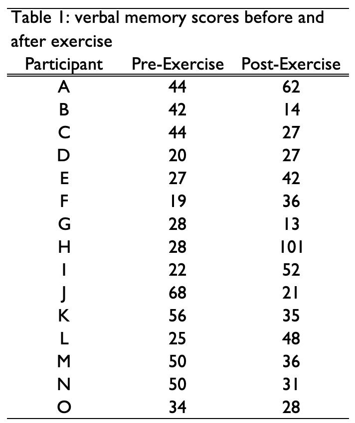
hippocampus (Kempermann, 2010), and memory testing (Rashidi, 2017). The hippocampal region specifically is significant due to its primary responsibility for storing and processing memories, along with generating new nerve cells (Biderman, 2020). The outcomes of these studies support the hypothesis that exercise can improve overall brain function, enhance memory, increase processing speed, and reduce the risk of dementia. With the extensive existing evidence linking physical activity to heightened brain health and function, it is reasonable to hypothesize that physical exertion will enhance brain function, specifically memory retention, and will be consistent with the findings from prior research. Although this research does exist, many of the experiments focus mainly on long-term programs, older adult populations, or animal models, leaving fewer studies that test the immediate, short-term cognitive changes in younger individuals. This study aims to examine whether a single bout of moderate physical exertion produces a short-term improvement in memory retention. The outcomes could determine practical application, whether brief physical activity, something students and workers could incorporate into daily routines, can enhance cognitive performance in real time. An example of real-life application could be performing light to moderate exercise before a test for students. Understanding the cognitive benefits of exercise is significant to clinical and non-clinical populations. This could also supplement current therapies as a tool for individuals who have conditions

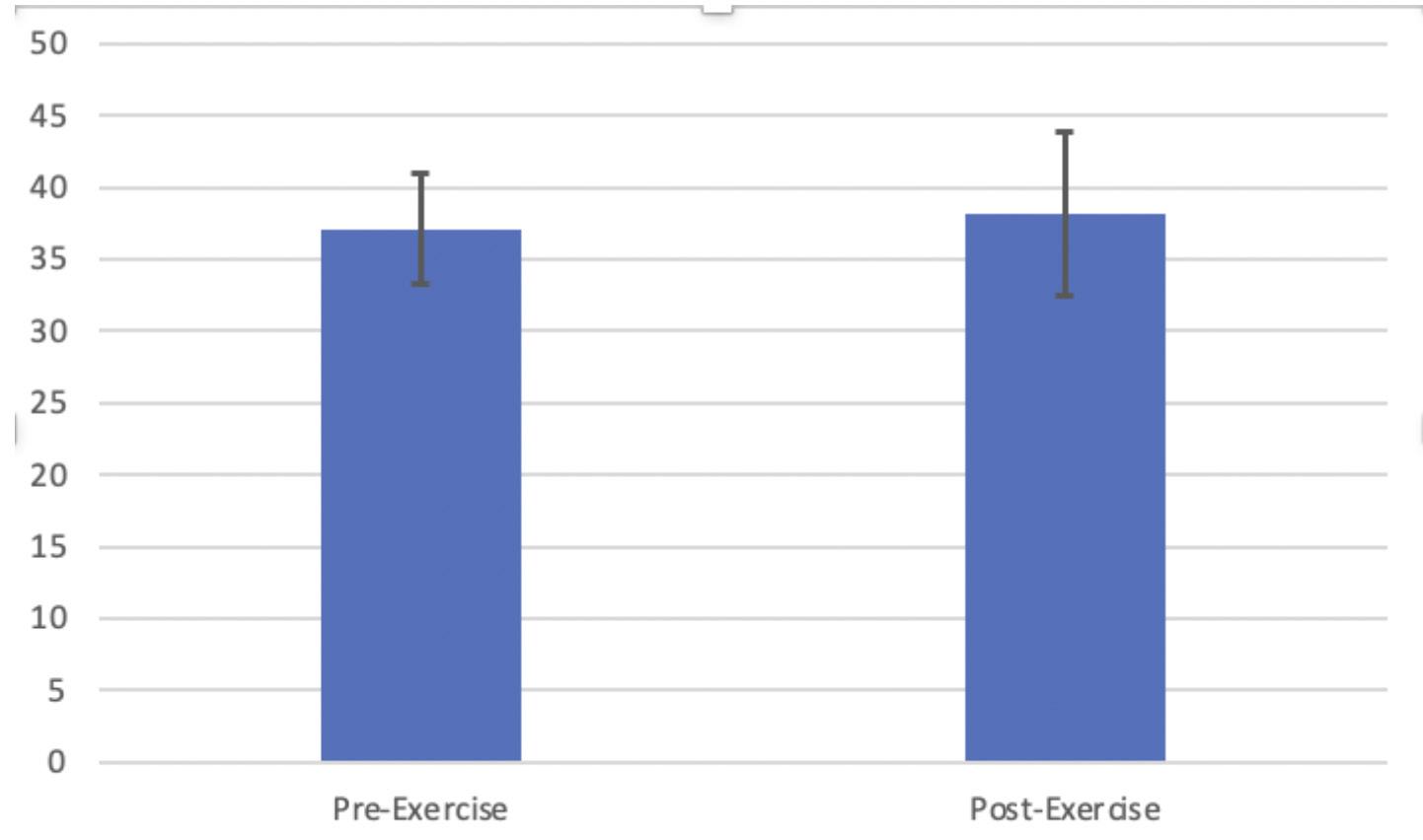
Fig. 2. Mean test score values before (pre-exercise) and after (post-exercise) activity. Error bars represent ± standard deviation.

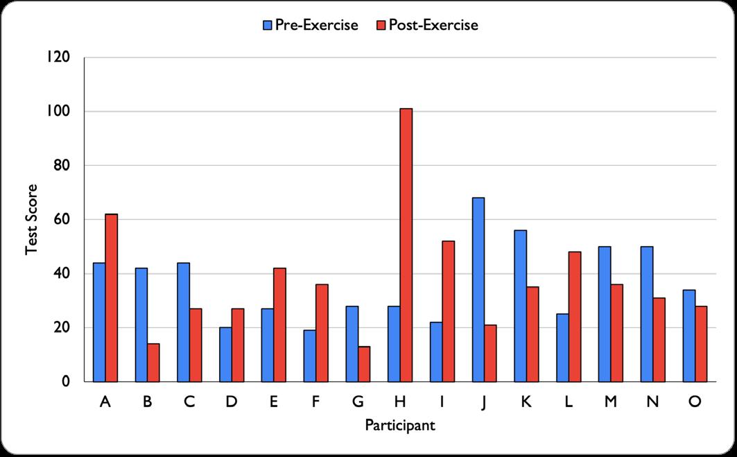
1: Comparison of average verbal memory scores before and after exercise.

such as ADHD, depression, and anxiety, as this population has demonstrated improved mental focus and emotional regulation in response to exercise interventions. Because exercise is easily accessible and associated with few or no negative side effects, it can be utilized as an effective and sustainable therapeutic tool to enhance cognitive function and overall mental well-being.

Methods

For this study, I used a group of 15 high school students, specifically female ice hockey players ages 15–18 years old, who had given informed consent. I tested their cognitive function before exercise using an online resource, the Human Benchmark Verbal Memory Test (Rashidi, 2017). The athletes engaged in one hour of on-ice cardiovascular exercise and were asked to repeat the cognitive test after exercise.The Human Benchmark Verbal Memory Test was an accessible online test designed to measure short-term memory and recognition ability for words. For this test, participants had to identify whether a presented word was new or previously seen. Performance was measured by the number of correct responses before three errors occurred. Once the participants completed the test, I collected their scores from both before and after exercise and compared the data using a paired t-test. This determined how many words each participant remembered before exercise and after exercise (Passell, 2019).

Results

The average verbal memory score before exercise was 37.93, while the average score after exercise was 35.13. A paired t-test showed that the difference was not statistically significant with a p-value of 0.58. Six participants saw improved scores after exercise, while eight participants saw a decline in their performance. Participant “H” was a major outlier in this experiment, with an initial score of 28 and a final score of 101, which was the biggest difference in scores. After utilizing the interquartile range test, it was confirmed that participant H was an official outlier. After removing participant H from the data set, the new pre-exercise mean was 37.79 and the post-exercise mean was 33.71 and the new p value of 0.46.

Discussion

The objective of this study was to determine the effects of strenuous exercise on short-term memory. After completing the procedure and analyzing the data, the results indicated that

Fig

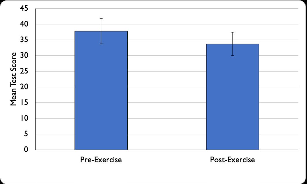
Fig. 3. Mean test score values after removing outlier, “Participant H”

the hypothesis was not supported (p = 0.58). The relatively high p-value suggests that there was no statistically significant difference between pre- and post-exercise scores. Although some participants saw an increase in scores (6 out of 15), a slightly larger number (8 out of 15) saw a decrease in scores post exercise, and the overall mean score decreased from 37.93 to 35.13. These findings suggest that cognitive function, specifically short-term memorization, may not be immediately enhanced after a single bout of strenuous exercise.

One limitation in this study was a notable outlier: “Participant H,” whose score increased from a 28 to a 101. After using the Interquartile Range Method, it was determined that the score of 101 was determined to be an outlier. It is possible that the participant may have had a misunderstanding of the initial test, improved understanding of the test post-exercise, and/ or inconsistent testing conditions. Other sources of error may include player fatigue post-exercise, changes in motivation, or external distractions. Furthermore, the small and limited sample size of strictly female hockey players of similar ages also made data application difficult, as it limited the generalizability of the findings to broader populations. Although my hypothesis was not supported, it is not uncommon to see similar outcomes in other studies that focus specifically on the immediate effects of exercise rather than long-term effects (Loprinzi et al., 2019). After further analysis of existing research, the results of this study align with the findings of a meta-study demonstrating that the effects of acute exercise on memory are heavily dependent on timing. Specifically, exercise can enhance memory in the early stages of consolidation, which can begin immediately after learning. Exercise immediately before or during learning, however, show little to no improvement, and even show some decline (Loprinzi et al., 2019). According to Nickerson (2025), strenuous exercise increases stress hormones such as epinephrine and cortisol, which may push the brain beyond its optimal level of cognitive performance, particularly during memory encoding and learning. This concept is explained by the Yerkes-Dodson Law, which suggests that cognitive performance peaks at moderate levels of physiological arousal but declines when stress levels become too high (Nickerson 2025). This study contributes to the greater body of scientific understanding on this topic because the majority of research done investigates the effects of long-term exercise and how sustained

The Effects of Acute Exercise on Cognitive Function

exercise programs can increase hippocampal volume, improve cerebral blood flow, and promote neurogenesis. However, fewer studies evaluate the immediate effects of a single exercise session on memory performance in adolescents. By focusing on shortterm cognitive changes in adolescent athletes, this study helps address the gap in inquiry and supports the limited existing research. In doing this study, it is possible now to look forward to possible future research, which could include expanding to a larger, more diverse sample size, including participants of different age groups, genders, or athletic backgrounds. Also, future studies could consider neurodivergent and neurotypical individuals to determine how the study differs among differing cognitive profiles. Furthermore, future studies could investigate the optimal timing and test different types of exercise, for example, aerobic vs. anaerobic, to determine how and when exercise most effectively enhances cognitive function. Understanding these mechanisms could help scientists develop evidence-based recommendations for students, athletes, and individuals with neurological or mental health conditions.

Works Cited

Erickson, K. I., Voss, M. W., Prakash, R. S., Basak, C., Szabo, A., Chaddock, L., … Kramer, A. F. (2011). Exercise training increases size of hippocampus and improves memory. Proceedings of the National Academy of Sciences of the United States of America, 108(7), 3017–3022.

Kempermann Gerd , Fabel Klaus , Ehninger Dan , Babu Harish , Leal-Galicia Perla , Garthe Alexander , Wolf Susanne Why and How Physical Activity Promotes Experience-Induced Brain Plasticity, Frontiers in Neuroscience, Volume 42010, 2010

Kinderman, P. (2014). The Drugs Don’t Work … So Offer Real Solutions. In: A Prescription for Psychiatry. Palgrave Macmillan, London. https://doi.org/10.1057/9781137408716_4

Konopka, Lukasz M. “How exercise influences the brain: a neuroscience perspective.” Croatian medical journal vol. 56,2 (2015): 169-71. doi:10.3325/cmj.2015.56.169

Maass, A., Düzel, S., Goerke, M., Becke, A., Sobieray, U., Neumann, K., Lövdén, M., Lindenberger, U., Bäckman, L., Braun-Dullaeus, R. C., Ahrens, D., Heinze, H. J., & Düzel, E. (2015). Vascular hippocampal plasticity after aerobic exercise in older adults. Molecular Psychiatry, 20(5), 585–593. https://www.ncbi.nlm.nih.gov/pmc/articles/PMC10203129/ Rashidi, M., Shahvaranian, M., Sedaghat, M. (2017). Ann Appl Sport Sci, 5(Special Issue): 67-72.

Talbot, J. S., Perkins, D. R., Tallon, C. M., Dawkins, T. G., M. Douglas, A. J., Beckerleg, R., Crofts, A., Wright, M. E., Davies, S., Steventon, J. J., Murphy, K., Lord, R. N., A. Pugh, C. J., Oliver, J. L., Lloyd, R. S., Ainslie, P. N., McManus, A. M., & Stembridge, M. (2023). Cerebral blood flow and cerebrovascular reactivity are modified by maturational stage and exercise training status during youth. Experimental Physiology, 108(12), 1500-1515. https://doi.org/10.1113/EP091279

Tomoto, Tsubasa et al. “One-year aerobic exercise increases cerebral blood flow in cognitively normal older adults.” Journal of cerebral blood flow and metabolism: official journal of the International Society of Cerebral Blood Flow and Metabolism vol. 43,3 (2023)

Wahl, M. (2011, March 30). Enhancing blood flow to exercising muscles. Muscular Dystrophy Association. https://www. mda.org/quest/article/enhancing-blood-flow-exercising-muscles

World Health Organization. (2022). Physical activity. https://www. who.int/news-room/fact-sheets/detail/physical-activity

Passell, E., Dillon, D. G., Baker, J. T., Vogel, S. C., Scheuer, L. S., Mirin, N. L., Rutter, L. A., Pizzagalli, D. A., & Germine, L. (2019). Digital cognitive assessment: Results from the TestMyBrain NIMH Research Domain Criteria (RDoC) field test battery report (Preprint). PsyArXiv. https://osf.io/preprints/ psyarxiv/dcszr_v1

Rashidi, M., Shahvaranian, M., Sedaghat, M. (2017). Ann Appl Sport Sci, 5(Special Issue): 67-72.

Loprinzi, P. D., Blough, J., Crawford, L., Ryu, S., Zou, L., & Li, H. (2019). The Temporal Effects of Acute Exercise on Episodic Memory Function: Systematic Review with Meta-Analysis. Brain sciences, 9(4), 87. https://doi.org/10.3390/brainsci9040087

Nickerson, Charlotte. “What Is the Yerkes-Dodson Law?” Simply Psychology, 14 Aug. 2025, https://www.simplypsychology. org/what-is-the-yerkes-dodson-law.html.

The Effects of Acute Exercise on Cognitive Function

RESEARCH & DISCOVERY

Effectiveness of Ice versus Heat Therapy for Muscle Soreness and Injury Recovery

Makayla Putney

Abstract

The use of ice and heat to treat minor soft tissue injuries and aid in soreness recovery is very common among the athletic and health care communities.While both ice and heat have benefits to assist muscle recovery, in this experiment, one big question was asked: Does one treatment show more effectiveness in reducing muscle soreness, improving flexibility, and the recovery of minor soft tissue injuries, mainly focusing on Delayed Onset Muscle Soreness (DOMS) in athletes? While better flexibility and a decrease in soreness levels were recorded for ice and heat compared to the control group, data showed no significant difference between all treatment groups. Further education and understanding are important to help improve recovery strategies and reduce downtime for athletes after intense training or injury.

Introduction

Delayed onset muscle soreness, known as (DOMS), and acute soft-tissue injuries are immensely common among athletes and active individuals. DOMS is induced from microscopic tears in the muscle fibers, which repair and grow after the initial tears leading muscles to grow larger and stronger Petrofsky et al., (2015). Two well-known uses for managing soreness and aiding in recovery are cryotherapy (ice) and thermotherapy (heat). Many, including coaches and athletes, often recommend ice for minimal swelling and pain, and heat for stiffness and increased tissue flexibility. However, effectiveness can vary on how long and how consistent they are applied to the injury (Huang et al., 2025).

Research has shown that both ice and heat have benefits to help the body’s natural functions and functional processes, with methods of use and timing playing a role in which is more effective. Chen et al. (2025) noted cold therapy can decrease discomfort by slowing tissue irritation if applied directly after activity. Petrofsky et al.(2015) noted heat therapy increases tissue metabolism which causes healing to occur more quickly along with reducing pain within the muscle. Current information supporting the use of both heat and cold, however, highlights a lack of consensus on which should be used over the other in specific recovery goals. Petrofsky et al.(2015) found both treatments reduce post-exercise soreness but in different functional ways towards the muscles. Wang et al. (2022) considered ten different interventions, including cold pack, hot pack, cryotherapy, ice massage, and passive recovery during the experiment, reporting that heat relieves pain more effectively early after exercise where cold is better for recovery later in the process. More specifically, they determined that hot- packs used within the first day may be more effective in reducing pain. Then later after the exercise and initial treatment with heat, an extreme cold (cryotherapy) would be beneficial. Hotfiel et al., (2025) studied how thermal therapies work to help with injuries in particular, examining how these therapies helped with multiple parts of the body like the repairing of the tissue, blood flow, inflammation, and metabolism. They explained thermal therapies help with muscle temperature, circulating the blood, and reducing inflammation from the initial injury, making heat a useful tool for

injury rehabilitation and management.

Many experimental studies have shown the physiological effects of heat and cold, however the effectiveness is expected to vary from athlete to athlete and according to the sport played. Understanding what athletes do on a regular basis is important because it allows for a better understanding of muscles being worked and how ice or heat can benefit their recovery time. Also, ice and heat are low-cost and very accessible so understanding their effectiveness for athletes can help better training and resources.

The objective of this study is to determine the effectiveness of ice versus heat therapy in reducing muscle soreness and assisting in recovery from soreness and minor soft-tissue injuries in athletes. High school athletes performed a strengthening workout in the experiment and will either ice or heat after for a set time before data of their soreness and flexibility will be recorded with a simple flexibility test where a picture of participants knee angle is captured and measured to find the angle of the joint. The angle will allow the flexibility of the muscle to be determined allowing a better understanding of which is more effective in recovery and soreness.

Data is going to be collected and analyzed in determining the percentage the treatment worked in helping recovery. The results taken from the test will then be compared to determine which treatment was more effective.

Methods

The study design is guided by findings from Petrofsky et al., (2015) and Wang et al., (2022), which detail physiological outcomes of thermal therapies. Information from Vrindten et al., (2025) and Hotfiel et al., (2025) will be used for scientific mechanisms.

To determine the effectiveness of ice versus heat therapy in reducing muscle soreness, an experiment was conducted among physically active people involved in a minimum of one sport. In the experiment, DOMS was induced with two fitness activities: 30 squats and 30 lunges, targeting the Quadricep muscle. Then the participants used either the ice or heat treatment for 15 minutes immediately after the activities. Participants applied a heat or ice pack on their quadricep muscle directly after performing the set exercises to ensure the ice testing is done correctly, as improper icing duration and timing can cause delay in tissue healing and potentially tissue death (Horschig et al., 2024). They also applied the treatments immediately after to reduce potential sources of error in the experiment. For the following three days after the treatment their muscle flexibility and soreness was tested by photographing the participants knee angle as they were in a laying position on their stomach with their knees so their feet were moving towards the gluteus maximus and calculated the knee flexion angle. Participants were also asked to rank their soreness each day following the initial day. This experiment was repeated to test the hot, cold, and control treatment. The experiment in total took about three-four weeks for all the testing to be done. Tests were done across four days for the experiment and the following days with no testing to allow the muscles to finish the process of repair and growth from microscopic tears in the fibers induced from working the quadriceps muscles. Data was entered into a spreadsheet throughout the duration of the experiment and after all testing was completed the data was graphed to visualize trends and then calculated for the One-Way ANOVA, Tukey HSD, and an independent sample T-Test, which was used to evaluate the effectiveness in soreness reduction and flexibility of muscles after heat and ice therapies.

Results

Pain Ratings

Soreness pain ratings peaked within the first 24 hours following exercise, consistent with established DOMS progression (Petrofsky et al., 2015). The control experiment exhibited the greatest peak in soreness and remained slightly higher than both treatments for the duration of the recovery period. The Ice treatment demonstrated the lowest peak at 24 hours (Figure one). At 48 hours, the heat treatment showed the lowest pain rating. Overall, all three treatments had similar patterns of soreness progression and recovery. Both the heat and ice treatments showed lower pain ratings. Soreness pain ratings gradually declined between 24 to 48 hours across all three treatments (Figure one). For the Pain Rating scale the heat treatment showed no statistical significance compared to the control group with a p-value of (p=0.120). The cold treatment showed statistical significance compared to the control group with a p-value of (p=0.038). Neither the heat nor cold treatment ]showed any significant difference between each other.

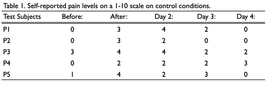
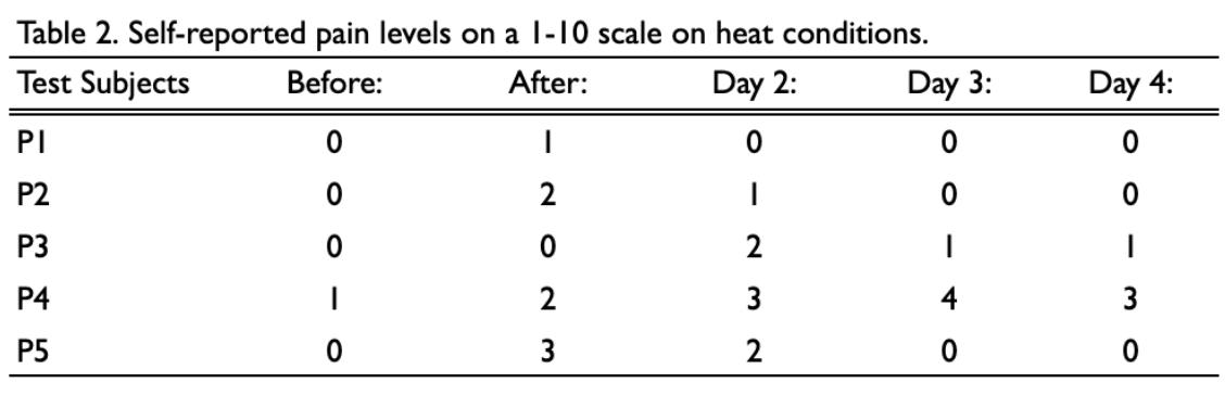
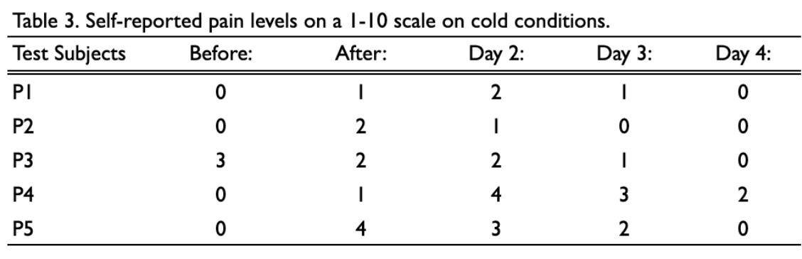
Knee Flexion Angle

The knee flexion angle was measured to indicate quadricep flexibility and stiffness, with lower angles representing greater flexibility. In the heat and ice treatments, quadricep flexibility immediately increased following exercise (figure two). Both treatments showed a minor decrease in flexibility between 24 to 72 hours (Figure two). The control treatment demonstrated a consistently greater angle, remaining above both heat and ice treatments for the duration of the experiment. The Ice treatment remained just below the heat treatment for the duration of the experiment, indicating the ice is properly manipulating the process of inflammation in soft tissue creating slightly greater flexibility in the quadricep muscle (Horschig et al., 2024). Overall, the heat and ice treatments had similar patterns for quadricep flexibility, while the control treatment remained divergent from the heat and

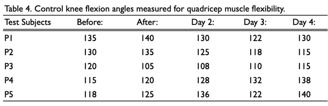
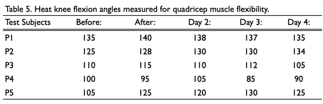
ice treatments. The cold had no statistically significant difference compared to the control group with a p-value of (p=0.038). Heat was not significantly different compared to the control group as well with a p-value of (p=0.487). The heat and cold treatments additionally did not show any significant difference between each other.

The testing concluded that while the cold and heat treatments showed lower pain ratings than the control group, the treatments did not show significant difference in the results. For Knee Flexion angle the cold showed better knee flexibility than heat however neither the cold or heat treatments showed any significant difference to the control group. The data shows that ice and heat treatments show improvement to the process of DOMS, there was no significant difference between the therapies and the control group.

Discussion

The purpose of this study was to test whether thermotherapy (heat) and cryotherapy (ice) were more effective in reducing muscle soreness and quadriceps flexibility after inducing Delayed Onset Muscle Soreness (DOMS). The results indicate that Ice and Heat had strong impacts on reducing pain and flexibility. Pain rankings followed the expected progression of DOMS, peaking within the 24 hour period and gradually declining through the 28 hour period. While minimal differences were observed between treatments there was not significant difference between the ice and heat treatment. That data demonstrates both ice and heat altered muscle soreness more compared to the control treatment but isn’t significant enough. These results match results with prior studies indicating that heat and cold can temporarily bring muscle relief (Petrofsky et al., 2015). Knee flexion angle measurements indicated small and consistent differences between ice and heat treatments. In the data, the lower knee flexion angles indicate greater quadriceps flexibility. The slightly lower values observed in the heat and ice treatments illustrate improved flexibility recovery compared to that of the control treatment. The trends of the data indicate that ice and heat contribute to improvements in muscle flexibility. Overall, both the thermotherapy and the cryotherapy reduced muscle soreness compared to the control treatment. However, heat showed the lowest soreness peak, the difference between heat and ice isn’t statistically significant. The data indicates that cold treatment had a substantially greater

effect on muscle flexibility.

Despite these results, several limitations should be considered when analyzing the data. The sample size for this experiment was (n=5), which reduces statistical power and limits generalizability to a greater population. Additionally, measurement error in knee flexion angle reading may occur, altering the data, and the seventy-two hour experiment duration may not have captured full recovery for all participants in the experiment.

In future research, experimentation should include a larger sample size with more athletic diversity and additional markers such as muscle thickness or electromyographic activity. Measuring the muscle thickness and electromyographic activity, provide direct structural and functional evidence of how the therapies change the muscle tissue, swelling, and muscle activation patterns. These tools for future studies would give more accurate data on the effect of either therapy on muscles. Extending the experiment duration beyond seventy-two hours may also provide more complete understanding of long-term treatment effects which would allow for a deeper grasp of the full recovery process of the muscle and insure complete recovery within the muscle. Overall, the findings suggest that while thermotherapy and cryotherapy do not significantly reduce muscle soreness compared to natural recovery, thermotherapy and cryotherapy provide a slight benefit in restoring quadriceps flexibility.

Works Cited

Chen, J., Hu, Q., Hu, J., Liu, S., & Yin, L. (2025). Differences in the effectiveness of different physical therapy modalities in the treatment of delayed-onset muscle soreness: A systematic review and Bayesian network meta-analysis. Journal of Pain Research, 18, 2993–3008.

Horschig, A., Sonthana, K., Williams, B., Horgan, M., & Starrett, K. (2024). The efficacy of icing for injuries and recovery — A clinical commentary. Journal of Contemporary Chiropractic, 7(1), 96–101. Journal of Contemporary Chiropractic Hotfiel, T., Engelhardt, M., Hammer, C., Grim, C., & Freiwald, J. (2025). Heat and cold therapy in sports – Rethinking mechanisms and clinical applications. Sports Orthopaedics and Traumatology, 41(1), 28–34.

Huang, Y.-C., Chou, T.-Y., Chen, T. C., & Chen, H.-T. (2025). Effect of cold-water immersion treatment on recovery from exercise-induced muscle damage in the hamstring. European

Fig. 2. Average soreness over time line graph with error bars representing standard error.

Fig. 2. Average flexibility over time line graph with error bars

Journal of Sport Science, 25(3), e12235.

Petrofsky, J. S., Khowailed, I. A., Lee, H., Berk, L., Bains, G. S., Akerkar, S., Shah, J., Al-Dabbak, F., & Laymon, M. S. (2015). Cold vs. heat after exercise — Is there a clear winner for muscle soreness? Journal of Strength & Conditioning Research, 29(11), 3245–3252.

Vrindten, K. L., Lonati, D. P., Mazzocca, J. L., & Matzkin, E. G. (2025). Thermal modalities including hot baths and cold plunges play a unique role in injury prevention and recovery. Arthroscopy, Sports Medicine, and Rehabilitation, 7(2), 101143.

Wang, Y., Lu, H., Li, S., Zhang, Y., Yan, F., Huang, Y., Chen, X., Yang, A., Han, L., & Ma, Y. (2022). Effect of cold and heat therapies on pain relief in patients with delayed onset muscle soreness: A network meta-analysis. Journal of Rehabilitation Medicine, 54, 331.

RESEARCH & DISCOVERY

Sunscreen Effectiveness: A Study of SPF Levels and Active Ingredients

Raylee Stearns

Abstract

Skin cancer is a huge global health issue and is oftentimes caused by ultraviolet (UV) radiation. Sunscreen is the most common way to protect yourself against damage, but questions remain about whether higher SPF numbers actually provide better protection or whether different active ingredients affect the level of protection. This study compared the effectiveness of mineral sunscreens, which use Zinc Oxide to reflect rays, against chemical sunscreens that use ingredients like Avobenzone and Homosalate to absorb them. To evaluate the relationship between types of active ingredients and protection levels, the experiment tested a range of different SPF ratings (15,30,50) for both a chemical sunscreen (Sun Bum) and a mineral sunscreen (Absolutely Natural). This study used Saccharomyces cerevisiae (yeast) as a model organism because its DNA repair process is very similar to how human cells react to UV damage. Each sunscreen was placed on petri dish lids over liquid yeast culture, exposed to UV, stained with methylene blue, then cells were counted using a hemocytometer. A Two-way ANOVA test showed sunscreen type (p<0.001) and SPF level (p=0.006) significantly affected yeast survival, mineral, and higher SPF levels protected cells the best.

Introduction

Skin cancer is one of the most common cancers worldwide, and the most common cause is exposure to ultraviolet radiation (Soehnge et al., 1997). Sunscreens are designed to protect the skin from the damaging UV rays that lead to mutations in skin cells and cancer development (Soehnge et al., 1997). These sunscreens are generally classified as chemical or mineral, depending on their active ingredients (Sorpese et al., 2007). Chemical sunscreens’ most common active ingredients include oxybenzone and avobenzone, which absorb UV radiation and convert it to heat, whereas mineral sunscreens’ common active ingredients include zinc oxide or titanium dioxide, which block and reflect the UV rays (Sorpese et al., 2007; Ginzburg et al., 2021). The active ingredients in chemical and mineral sunscreens differ, as do their approaches to protecting the skin. SPF refers to the percentage of UV rays it protects against; for example, UV 30 only allows 1/30 of UV rays to penetrate the protective layer (Bissonauth et al., 2000).

Questions remain concerning the effectiveness of chemical vs mineral sunscreen, and if a higher sun protection factor, more commonly known as SPF rating, actually provides more protection against the damaging rays, or if it’s a marketing strategy used by companies to increase profits. A study found that SPF 100 sunscreen provided better protection against sunburn and UVinduced erythema, characterized by skin turning red, than SPF 50 during a 5-day study conducted at the beach (Kohli et al., 2020). Participants experienced more sunburn on the side with SPF 50, consistent with more erythema than the side with SPF 100 (Kohli et al., 2020). These results show that higher SPF sunscreens provide more protection when exposed to UV radiation, but I wonder if sunscreen was applied constantly as recommended and applied using the proper amount recommendation. Additionally, some sunscreens with the same SPF labels can vary in sun protection depending on the brand (Hojerová et al., 2011). This study makes me wonder if the SPF protection varied because of the active ingredients or because of something like a source of error in the study. Additionally, broad-spectrum sunscreens, which protect against UV A and UV B rays and can be chemical

or mineral, have been found to prevent DNA damage caused by UV exposure (Ambruso et al., 2023). Recent research has found that mineral sunscreens may undergo structural changes when they are exposed to UV radiation, which may alter their effectiveness (Ginzburg et al., 2021). This study aims to evaluate a variety of sunscreens in an attempt to evaluate the source of these inconsistent findings.

To study sunscreen effectiveness in a controlled system, I used Saccharomyces cerevisiae (yeast) as a model organism to mimic human cells. Yeast DNA repair mechanisms are similar to those found in human cells. A previous experiment tested SPF 15 and 50’s effectiveness on yeast (D’Costa & Santoro, 2008). So I plan to expand on this study by determining if SPF levels offer a significant increase in protection against UV rays, and if the active ingredients in these sunscreens play a significant role.

This research is important to determine if higher-priced or mineral options, which are better for the environment, provide better protection and to identify which type most effectively prevents UV-related skin damage and cancer.

The study’s objective is to assess the effectiveness of

sunscreens with different SPF ratings and active ingredients when studying how well they protect yeast cells from UV damage. It is hypothesized that higher SPF sunscreens and mineral-based formulas will provide greater protection to the yeast cells, which will result in a higher survival rate of the yeast colonies after exposure to UV rays compared to those treated with chemical or lower-rated SPF.

Methods

For my experiment, I used yeast as an organism to evaluate the effectiveness of chemical and mineral sunscreens at different SPF levels (15,30,50) in preventing damage when the yeast is exposed to UV radiation. I began this experiment by placing 0.25 grams of yeast in a mason jar with 0.5 grams of sugar and 100 ml of water. I heated it to 32-38 degrees Celsius, then allowed it to grow in the jar covered with plastic wrap for 10-20 minutes (Alhamdy & Al-Sowayan, 2020). I then took two mL of the liquid yeast culture and placed it in small petri dishes. I conducted this experiment over three days, and each day I had eight petri dishes prepared, one for my positive control (SPF 0), one for my negative control (UV 0), three for my mineral sunscreens, and three for my chemical sunscreens. For my Chemical sunscreen, I used Sun Bum, and the active ingredients were Avobenzone, Hemosalate, Octisalate, and Octocrylene with different concentrations for each SPF value (Table 1). For my mineral sunscreen, I used the brand Absolutely Natural, and the active ingredient was Zinc Oxide with different concentrations for each SPF value (Table 2). I treated my petri dishes with sunscreen by smearing the specific sunscreen on the lids with a butter knife. I then tested the UVI of my 100w Lucky Herp reptile mercury vapor lamps by using a UVI sensor and recorded UVI values fluctuating between UVI 0-12 at approximately 22 centimeters from our petri dishes, which were placed on a one-inch stand made of cardboard to prevent the table from getting too hot. I placed my petri dishes at randomly assigned positions, to control for varying UV intensity relative to distance from the center of the light, under these two lamps for 30 minutes. Then, after the 30 minutes were up, I took the petri dishes and randomly selected them to be viewed with our microscope and hemocytometer slide by first mixing 400 microliters of the liquid culture and 400 microliters of Methylene blue 0.1% concentration. After mixing my liquid culture with the methylene blue, I took 100 microliters of the mixed solution and placed it on my hemocytometer slide for viewing. I counted five squares for each liquid culture, counting the living, clear cells,

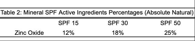
and not counting the dead, blue cells. I selected one square from each corner and one from the middle of the hemocytometer’s field of view to limit bias. I recorded the values and continued this process for all of my cultures mixed with methylene blue. After three days of recording data, I took all the data and placed it in a Google Sheet. I used the sheet to calculate the average survival for each group across the three separate days of testing. I conducted this test over three days to ensure correct counting via the hemocytometer, as well as making the results less biased because I did one of each three SPFs (15,30, and 50) per day. To make the data more comparable, I converted the numbers into percentages of the negative control group’s growth, which allowed me to normalize the data across the three separate days of testing. Doing so allowed for any daily variations in the baseline yeast growth or starting culture concentration. By setting the negative control as the 100% baseline, I could accurately isolate and measure the exact percentage of cell growth achieved after UV radiation as well as the level of protection provided by each sunscreen type and SPF level. I then moved the data into Excel to create a bar graph and add error bars to the graph to account for the variation in the results and how much the survival counts changed between the trials. Finally, to see if my results were significant, I used Google’s Gemini AI to run a “Two-way ANOVA” test. A two-way ANOVA tests how two different factors affect a result, both separately and together (Numiqo Team, 2025). My two factors were the type of sunscreen (Chemical vs. Mineral) and the SPF levels (15,30,50)

Results

The results of the experiment involve measuring the percentage of cell growth in comparison to the unexposed negative control. The data in Figure 1 and Table 3 show that both sunscreen type and SPF level play a role in the yeast colony’s survival. In my analysis, the mineral sunscreen (Absolutely Natural) consistently resulted in a higher percentage of living cells, signifying cell growth in comparison to the chemical sunscreen (Sun Bum) at every SPF level. The highest cell count was seen in the Mineral 50 group, which averaged approximately 115% of the negative controls’ growth, meaning that the average cell count of the Mineral 50 treatment exceeded the average cell count by 15% of the negative control. Mineral 30 also had a significantly higher

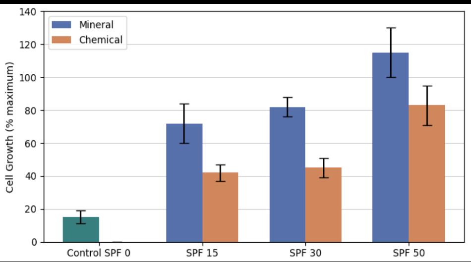
Fig. 1. Average percent of yeast cell growth compared to the unexposed negative control across the different sunscreen types and SPF levels. Error bars represent the standard error of the mean between the trials

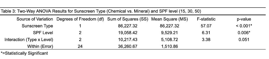
cell count than most of the other treatments, with approximately 82% of the negative controls’ growth. Chemical 15 and 30 groups showed the lowest percent of growth, both falling below 45% of the negative control’s growth. The error bars in figure one show the standard error of the average between the three separate trials, all happening on different days. The statistical significance of these results is shown in the two-way ANOVA analysis (Table 1). The effects of the sunscreen type were very significant (F = 57.07, p < 0.001) as well as the effect of the SPF level (F = 6.31, p = 0.006). The interaction between the two variables resulted in a p-value of 0.051, suggesting that the two factors influenced the growth percentages independently. While 0.051 is technically just above the standard of 0.05 cutoff for statistical significance, the proximity of the cutoff does still suggest a strong pattern. This indicates that the relationship between the type of sunscreen and its SPF level most likely has a combined effect on yeast survival.

Discussion

The objective of this study was to evaluate the effectiveness of sunscreens with varying Sun Protection Factor (SPF) ratings and active ingredients in protecting yeast cells from UV damage. It was hypothesized that higher SPF ratings and mineral-based formulas would provide greater protection to the yeast cells, which would result in a higher survival rate of the yeast colonies after exposure to UV rays compared to those treated with chemical or lower-rated SPF. The data supported this hypothesis as mineral sunscreens outperformed chemical sunscreens at every SPF level tested, including 15, 30, and 50. The mineral SPF 50 group achieved the highest survival rate at approximately 115% relative to the negative control, and mineral 30 achieved 82% of the negative control’s growth. This indicates that the mineral SPF 50 treatment not only prevented damage but may have slightly enhanced cell viability compared to the negative control, resulting in a value above 100%. Chemical 15 and 30 both had less than 45% of the negative control growth, showing a lack of protection in comparison to the mineral sunscreens. These findings were statistically significant as supported by a two-way ANOVA test, which showed significant effects for both sunscreen type (p<0.001) and SPF level (p=0.006). The results suggest that SPF and active ingredients interact to influence overall protection. That being said, the survival rate exceeding 100% in the mineral group suggests errors that could have been made, like the mineral layer being thicker, manual cell counting error, or maybe suggesting that it improves growing conditions for the cells, and lastly, maybe a lack of randomization of counting order. This may also indicate that the negative control was not a true representation of the baseline; it may have been an underestimate, which led to the treatment’s survival values being exaggerated. To address these issues in future studies, the amount of sunscreen should be measured and consistent between all tests,

three people could count the same sample and average them to get a more accurate cell count, and a randomized counting order should be implemented to prevent bias from influencing the results. These changes would improve the reliability of our results. This research provides important context for the study of skin cancer prevention by identifying which active ingredients best protect DNA against UV-induced damage. The results also align with other studies that agree mineral sunscreens, which reflect UV rays, are more effective than chemical sunscreens, which absorb UV rays (Sorpese et al., 2007). Similarly, the results align with previous studies that higher SPF levels provide more adequate protection (Kohli et al., 2020). This supports using yeast as a model organism because it responds to UV similarly to how human cells react in previous studies (D’Costa & Santoro, 2008). Future studies should transition to human cells, or better yet, human skin models, because the response to radiation and DNA damage in humans will likely differ from the reactions observed in yeast.

Acknowledgments

This study was supported by funding from the Allendale Columbia School. I would like to acknowledge Mr. Godkin as well as Gabby Giambra for their valuable insight and assistance in conducting the experiment.

Works Cited

Ambruso, K., Park, H.-Y., & Riley, K. R. (2023). Analysis of the active ingredients in sunscreen: A multiweek experiment for the analytical chemistry laboratory. Journal of Chemical Education, 100 (12),4845–4852. https://pubs.acs.org/doi/ full/10.1021/acs.jchemed.3c00808

Bissonauth, V., Drouin, R., Mitchell, D. L., Rhainds, M., Claveau, J., & Rouabhia, M. (2000). The efficacy of a broad-spectrum sunscreen to protect engineered human skin from tissue and DNA damage induced by solar ultraviolet exposure. Clinical Cancer Research, 6, 4128–4135. https://aacrjournals.org/clincancerres/article/6/10/4128/287908/The-Efficacy-of-a-Broad-spectrum-Sunscreen-to

D’Costa, A. R., & Santoro, I. (2008). The effect of UV radiation on the survival of yeast and its implications for a real-life situation. ABLE 2008 Proceedings, 30, 372–382. https://www. ableweb.org/biologylabs/wp-content/uploads/volumes/ vol-30/029.pdf

Ginzburg, A. L., Blackburn, R. S., Santillan, C., Truong, L., Tanguay, R. L., & Hutchison, J. E. (2021). Zinc oxide–induced changes to sunscreen ingredient efficacy and toxicity under UV irradiation. Photochemical & Photobiological Sciences, 20, 1273–1285. https://doi.org/10.1007/s43630-021-00101-2

Hojerová, J., Medovcíková, A., Mikula, M., Sovciková, D., & Chmelík,

M. (2011). Photoprotective efficacy and photostability of fifteen sunscreen products having the same label SPF subjected to natural sunlight. International Journal of Pharmaceutics, 408(1–2), 27–38. https://doi.org/10.1016/j. ijpharm.2011.01.040

Kohli, I., Nicholson, C. L., Williams, J. D., Lyons, A. B., Seo, I., Maitra, P.,(...), Hamzavi, I. H. (2020). Greater efficacy of SPF 100+ sunscreen compared with SPF 50+ in sunburn prevention during 5 consecutive days of sunlight exposure: A randomized, double-blind clinical trial. Journal of the American Academy of Dermatology, 82(4), 869–877. https://doi. org/10.1016/j.jaad.2019.09.018

Numiqo Team. (2025). Two-way ANOVA. numiqo: Online Statistics Calculator. numiqo e.U. https://numiqo.com/tutorial/two-factorial-anova-without-repeated-measures

Sorpese, N., Dondi, D., & Albini, A. (2007). Inorganic and organic UV filters: Their role and efficacy in sunscreens and suncare products. Inorganica Chimica Acta, 360(3), 794–802. https://doi.org/10.1016/j.ica.2005.12.057

RESEARCH & DISCOVERY

Salivary biomarkers and Early Prediction of Atopic Dermatitis in Infancy

Chloe Terio

Abstract

Atopic dermatitis (AD) is a common inflammatory skin condition that often begins in early childhood, but tools to predict it before symptoms appear are limited.This study investigated whether salivary biomarkers, including immune markers and the oral microbiome, are associated with the development of AD in early infancy. A cohort of 119 infants was followed from birth to 24 months, with saliva samples collected at multiple time points and analyzed for immune markers and microbial composition.While there was no difference in overall microbial diversity, beta diversity differed significantly at two months (p = 0.038), suggesting early differences in bacterial composition. Infants who later developed AD showed higher levels of the immune markers IL-1a and IL-9 at four months and lower IL-1a at six months. These findings suggest that salivary biomarkers are associated with the development of AD and may serve as a noninvasive tool for early detection of disease risk.

Introduction

Atopic dermatitis (AD), also known as eczema, is one of the most common chronic inflammatory skin diseases, typically emerging in early childhood and often persisting into adulthood (Ständer, 2021). AD causes itchy, red, and irritated skin that often flares up in cycles. It is also connected to other allergic conditions like asthma and hay fever, which together make up what is known as the “atopic march.” Globally, AD has increased over recent years, affecting up to around 25% of children and about 2-3% of adults (Eichenfield et al., 2014).The causes of AD are complex and involve a mix of genetics, immune system imbalance, skin barrier problems, and environmental triggers (Bakker et al., 2023).

Because AD varies so much from person to person, researchers have focused on identifying biomarkers. Specifically, measurable biological indicators that can help predict or track disease development. Biomarkers have advanced our understanding of AD’s underlying causes and could support earlier diagnosis and more precise treatments. For instance, skin biomarkers have been shown to predict the likelihood of developing AD during infancy (Rinnov et al., 2022). Additionally, studies have found that microbial communities, especially those under the skin, may influence immune activity and disease severity, showing that changes in the microbiome could be an early sign of AD risk (Zhang et al., 2024).

Saliva is emerging as an especially promising tool for studying early-life health because it is noninvasive, easy to collect, and rich in information. It contains immune-related molecules such as cytokines and antibodies, as well as microbial DNA that reflects both oral and systemic health (Zainal et al., 2021). These features make saliva an ideal method for identifying early immune or microbial markers associated with AD.

Since saliva also carries microbes from the mouth, it can help show what is happening in the oral environment. The oral microbiome is one of the body’s most diverse microbial communities. It includes over 700 species of bacteria, as well as fungi and viruses, all of which contribute to immune regulation and systemic health (Deo & Deshmukh, 2019). This community plays a key role in both oral and systemic health. Early colonization of the mouth by microbes may help train the immune system, while

imbalances in these microbes have been linked to inflammatory and allergic conditions. A 2024 study found that children with AD had different microbial patterns not only on their skin but also in their saliva and gut (Zhang et al., 2024), suggesting that oral microbes could influence immune development and allergic disease.

While much research has focused on the gut microbiome and blood-based immune markers in AD, little is known about how salivary biomarkers reflect or predict the disease. Since saliva contains both immune and microbial signals, it might help identify early signs of AD risk in infants. Understanding these patterns could lead to noninvasive, early detection strategies and, in the future, more specific prevention for children who are likely to develop AD.

The objective of this study is to assess how differences in salivary biomarkers, such as immune markers and changes in the oral microbiome, relate to the onset or severity of atopic dermatitis in early infancy. By analyzing saliva samples from infants with and without AD, this study aims to identify distinct biomarker patterns that could serve as early warning signs of the disease and evaluate saliva’s potential as a simple, noninvasive tool for early detection and risk prediction. We hypothesize that specific salivary biomarkers reflecting immune and microbial changes are associated with AD and may serve as early indicators of disease development.

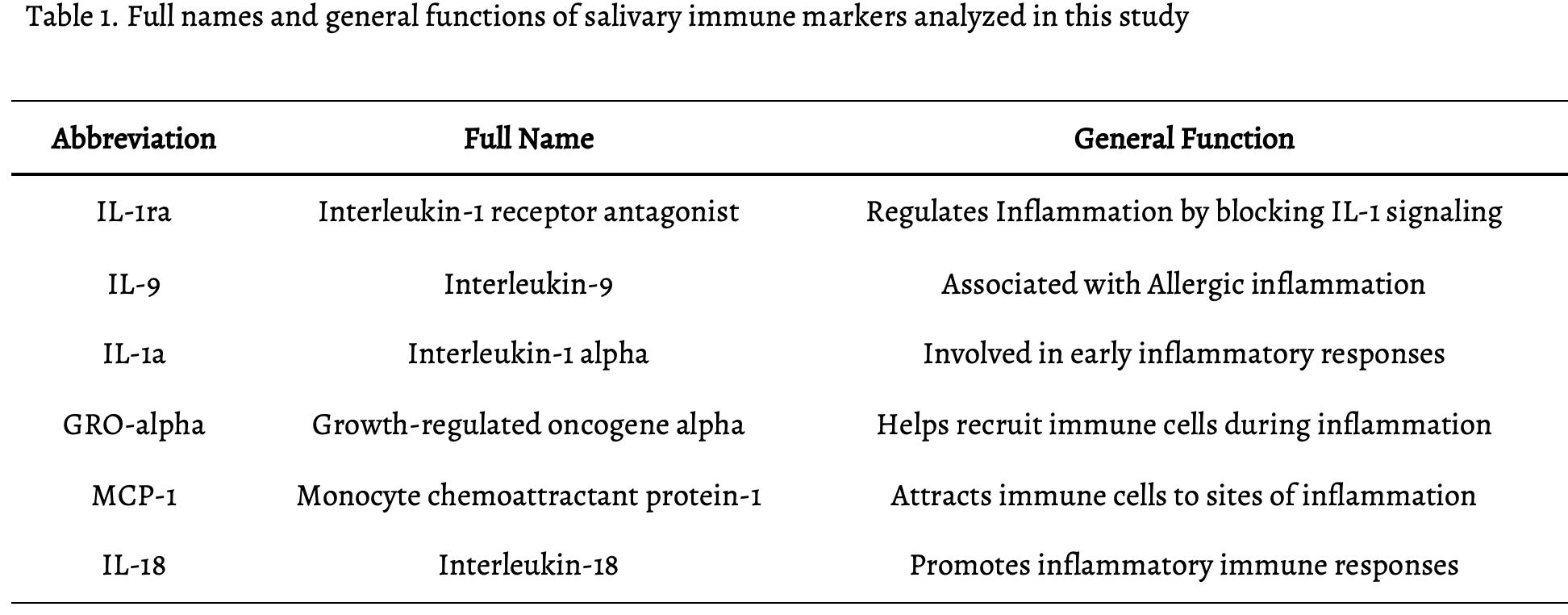
Methods

This study was part of a larger mother-infant birth cohort that followed 160 babies from clinics at the University of Rochester between 2018 and 2023. Each infant was tracked for the first two years of life. Babies were not included if they were born early, had low birth weight, Down syndrome, cleft lip or palate, or had taken antifungal medications. All study procedures were approved by the University of Rochester’s research board and followed official reporting guidelines (Alkhars et al., 2025).

We collected saliva from each infant at 1 week and at 2, 4, 6, 12, 18, and 24 months. Samples were kept cold and stored at -80 °C. Families also provided information about their background, medical history, feeding routines, and oral health habits. Using zip codes, we obtained additional info on each family’s community environment. Similar studies have used saliva-based immune and inflammatory biomarkers in infants and young children to assess immune functioning, supporting the validity of these methods (Riis et al., 2017).

To determine which children had AD, we checked the electronic health records and confirmed diagnoses made by doctors. For saliva, we measured 36 immune markers, including cytokines and growth factors, using the MILLIPLEX® magnetic bead-based immunology panel. We also measured six hormones in saliva using a magnetic bead assay on a Luminex machine. DNA was extracted using a Qiagen kit, and sequencing libraries were prepared and run on an Illumina Novaseq machine. Afterward, we analyzed the sequencing data using bioinformatics tools such as MetaPhlAn to classify bacterial types and determine how common they were in each sample. These biomarkers were measured as quantitative values, and we compared them between infants who developed atopic dermatitis and those who did not to determine whether there were statistically significant connections. Statistical comparisons between groups were done using independentsamples t-tests for alpha diversity and immune markers, and PERMANOVA for beta diversity, with p-values < 0.05 considered statistically significant.

Results

Timing of AD development during early infancy

Among the 119 infants included in this study, 48% developed atopic dermatitis (AD) within the first two years of life. Most

Fig. 1. Timing of Atopic Dermatitis Development in infants during the first two years

cases appeared during early infancy (Figure 1). The highest number of new cases occurred between months two and four, with about 8% of infants developing AD at month two and around 7-8% at months three and four. By six months of age, about 34% of infants had developed AD. This number increased to 42% by 12 months. After the first year, the number of new cases slowed down, with only about 6% of infants developing AD between 13 and 24 months. These results show that AD often begins early in life, highlighting the importance of studying biological markers during the first year.

Salivary Microbiome and bacterial differences

We examined whether the salivary microbiome differed between infants who developed AD and those who did not. Overall bacterial diversity within the sample (Alpha diversity), which measures how many different bacterial species are present and how evenly they are distributed, was calculated using the Shannon index (Figure 2A) and did not differ significantly between the two groups at any time point (independent samples t-test, p > 0.05).

Beta Diversity, which measures differences in the total microbial community between individuals, showed a significant difference at 2 months of age (PERMANOVA; p = 0.038) between infants who developed AD by 1 year and those who did not (Figure 2B). No significant differences were observed at the other time points.

Fig. 2. Differences in Salivary Microbiome Diversity between infants with and without AD.

(A) Alpha diversity of the salivary microbiome, measured using the Shannon index, is shown with each point representing one infant. Higher values indicate greater bacterial diversity, while lower values indicate less diversity. There were no significant differences between infants who developed AD and those who did not at any time point (independent samples t-test, p > 0.05).

(B) Beta Diversity, measured using the Bray-Curtis dissimilarity index, is shown in a scatter plot where each point represents one infant. Points closer together have more similar bacteria, while points farther apart are more different. The x-axis and y-axis explain 44.1% and 22% of the variation in the microbial data, respectively. The groups are somewhat separated at 2 months, showing a difference between infants with and without AD (PERMANOVA, p = 0.038).

Salivary Immune Markers Associated with AD

Several differences in salivary immune markers were observed between infants who developed AD by one year and those who did not (Figure 3; Table 1). Some of these differences appeared before AD was diagnosed. At 4 months of age, infants who later developed AD had higher levels of IL-1ra (p = 0.024) and IL-9 (p = 0.034). At 6 months, IL-1a levels were significantly lower in infants who developed AD (p = 0.038). At 12 months, GRO-alpha levels were also lower in infants with AD (p= 0.044). MCP-1 levels showed a similar trend at 12 months but did not reach statistical significance (p = 0.054). At 24 months, infants with AD continued to show lower levels of IL-1a (p = 0.048) and IL-

Fig. 3. Differences in Salivary Immune Markers Between Infants with and without AD.

This figure compares levels of immune markers between infants who developed atopic dermatitis (AD) and those who did not at different ages. Each point represents one infant, and higher or lower positions indicate higher or lower levels of the immune marker. P-values show whether the differences between the groups were statistically significant. Infants who developed AD showed differences in several immune markers, including higher IL-1ra and IL-9 at 4 months; lower IL-1a at 6 months; lower GRo-alpha at 12 months; and lower IL-1a and IL-18 at 24 months.

18 (p = 0.033). These findings suggest that differences in salivary immune markers may be associated with the development of AD during early infancy.

Discussion

The objective of this study was to determine whether salivary biomarkers, including immune markers and the oral microbiome, are associated with the development of atopic dermatitis (AD) in early infancy. The results support our hypothesis, showing that infants who developed AD had noticeable differences in both their immune markers and microbiome compared to those who did not. The data showed that AD mainly develops early in life, with most cases happening within the first year and peaking between two and four months. This suggests that early infancy is a critical period for the development of AD. In terms of the microbiome, there was no difference in alpha diversity, but beta diversity was significantly different at 2 months (p = 0.038), suggesting that the types of bacteria present early in life may be linked to AD risk. There were also differences in immune markers. Immune markers are molecules such as cytokines that help the body

control inflammation and respond to infections. Infants who later developed AD had higher levels of IL-1ra and IL-9 at 4 months and lower levels of IL-1a at 6 months, along with additional differences at later time points. These changes suggest that the immune system may be responding differently in infants, even before any visible symptoms of AD appear. This finding aligns with previous research, as IL-9 has been associated with allergic inflammation and conditions such as asthma and atopic dermatitis (Ciprandi et al., 2012). IL-1ra is also important because it helps block IL-1 signaling and can increase when the body is trying to regulate inflammation (Arend, 2002). IL-1a, on the other hand, is involved in early inflammatory responses in the skin, so lower levels at 6 months may suggest a change in skin-related immune signaling (Di Paeolo & Shayakhmetov, 2016). Since the immune system is still developing in infancy, differences in these cytokines may help explain why certain infants are more likely to develop AD.

These findings suggest that saliva may be a useful noninvasive tool for early detection of AD risk. Because saliva is easy to collect and does not require invasive procedures, it could continue to be used to monitor infants and identify factors linked to disease development. A limitation of this study is that salivary biomarkers may be influenced by external factors such as diet or oral hygiene, which could affect biomarker levels and increase variability in results. In addition, the sample size of 119 infants, while sufficient to detect some differences, remains relatively limited and may reduce the applicability of the findings. Additionally, because the study population was from a specific geographic and clinical setting, the results may not fully represent broader or more diverse populations. Finally, this study shows only a relationship between biomarkers and AD, not a direct cause, meaning the identified biomarkers may not directly cause AD.

These results contribute to existing research by supporting the link between immune and microbial changes to AD. This study is essential, as it contributes to current knowledge by showing that these changes can be detected in saliva in early infancy. Although biomarkers cannot be directly modified, future research could explore how they may be indirectly influenced by factors such as diet, oral hygiene, or environmental exposures that affect the immune system. Future studies should first confirm these findings in larger, more diverse populations and see how these biomarkers change over time. Researchers could then identify which factors most strongly influence biomarker levels before exploring whether targeted help could reduce the risk or severity of AD. In conclusion, this study provides evidence that salivary biomarkers are associated with the development of atopic dermatitis in early infancy and may serve as a useful tool for early detection.

Works Cited

Alkhars, N., Manning, S., Al Jallad, N., Zeng, Y., Wu, T. T., Fogarty, C., Mendoza, M., van Wijngaarden, E., Kopycka-Kedzierawski, D. T., Billings, R., Fiscella, K., Koo, H., & Xiao, J. (2025). Birth cohort study identifies Candida albicans as a risk factor for dental caries. Journal of Dental Research, 104, 1470–1478.

Arend, W. P. (2002). The balance between IL-1 and IL-1Ra in disease. Cytokine & Growth Factor Reviews, 13(4–5), 323–340.https://doi.org/10.1016/S1359-6101(02)00020-5

Bakker, D., de Bruin-Weller, M., Drylewicz, J., van Wijk, F., & Thijs, J.

(2023). Biomarkers in atopic dermatitis. Journal of Allergy and Clinical Immunology, 151(5), 1163–1168. https://www. jacionline.org/article/S0091-6749(23)00143-4/fulltext

Ciprandi, G., De Amici, M., Giunta, V., Marseglia, A., & Marseglia, G. (2012). Serum interleukin-9 levels are associated with clinical severity in children with atopic dermatitis. Pediatric Dermatology, 30(2), 222–225.https://doi.org/10.1111/ j.1525-1470.2012.01766.x

Deo, P. N., & Deshmukh, R. (2019). Oral microbiome: Unveiling the fundamentals. Journal of Oral and Maxillofacial Pathology, 23(1), 122–128. https://doi.org/10.4103/jomfp. JOMFP_304_18

Eichenfield, L. F., Tom, W. L., Chamlin, S. L., Feldman, S. R., Hanifin, J. M., Simpson, E. L., …Sidbury, R. (2014).Guidelines of care for the management of atopic dermatitis: Section 1. Diagnosis and assessment of atopic dermatitis. Journal of the American Academy of Dermatology, 70(2), 338–351. https://doi.org/10.1016/j.jaad.2013.10.010

Di Paolo, N. C., & Shayakhmetov, D. M. (2016).Interleukin 1α and the inflammatory process. Nature Immunology, 17, 906–913.https://doi.org/10.1038/ni.3503

Riis, J. L., Granger, D. A., DiPietro, J. A., Bandeen-Roche, K., & Johnson, S. B. (2015). Salivary cytokines as a minimally invasive measure of immune functioning in young children. Developmental Psychobiology, 57(2), 153–167. https://doi. org/10.1002/dev.21271

Rinnov, M. R., Halling, A.-S., Knudgaard, M. H., Vestergaard, C., & Johansen, J. D. (2022). Skin biomarkers predict the development of atopic dermatitis in infancy. Allergy, 77(12), 3649–3660.https://doi.org/10.1111/all.15518

Ständer, S. (2021). Atopic dermatitis. The New England Journal of Medicine, 384(12), 1136–1143.https://doi.org/10.1056/ NEJMra2023911

Zainal, N. H. M., Abas, R., & Mohamad Asri, S. F. (2021). Childhood allergy disease, early diagnosis, and the potential of salivary protein biomarkers. Mediators of Inflammation, 2021, Article 9198249. https://doi.org/10.1155/2021/9198249

Zhang, X., Huang, X., Zheng, P., Liu, E., Bai, S., Chen, S., Pang, Y., Xiao, X., Yang, H., & Guo, J. (2024). Changes in oral, skin, and gut microbiota in children with atopic dermatitis: A case-control study. Frontiers in Microbiology, 15, 1442126. https://doi.org/10.3389/fmicb.2024.1442126

RESEARCH & DISCOVERY

A Performance Review of Nozzle Geometries in Pulsed Plasma Thrusters

Nathan Thornburg

Abstract

This review focuses upon unique electrode geometries for ablative pulsed plasma thrusters, specifically variations of the rectangular and coaxial configurations. Currently many microsatellites lack propulsion systems and thus are unable to maintain or change their orbit. This review is a synthesis of literature relevant to our goal of realizing the different applications of these geometries for further use of these thrusters in spacecraft. The rectangular rail geometry possesses one of the longest lifespans, lowest cost, and greatest reliability of any geometry making it an ideal choice for implementation as reaction control systems in larger satellites. The coaxial nozzle configuration is overall less fuel efficient but produces a larger impulse, making them a better choice for use in microsatellites in which maneuvers of larger magnitude are being attempted.

Introduction

As the space industry continues to grow, it has become increasingly privatized, shifting away from previously government and state-funded research and missions (NASA, ESA, JAXA, etc.). Companies such as SpaceX, Blue Origin, Axiom Space, and Boeing have become major service providers for moving goods and people between Earth and space, thereby driving growth across the entire space industry. Thus, as a result of a growing industry, there are increasingly more opportunities for small organizations and researchers to buy space aboard rockets from private companies in order to launch their own spacecraft and lead their own missions. These privately owned and operated missions primarily utilize miniature satellites and spacecraft due to their lower fabrication and launch cost (often determined by the weight of the payload). As a part of this trend, microsatellites, categorized as satellites between 11 and 200 kilograms in weight, have increasingly grown in popularity among researchers and businesses interested in space flight due to their relatively minimal production, launch, and maintenance costs. Unfortunately, as a direct result of these satellites’ small size, most reside in low Earth orbit with a lack of proper attitude control or station-keeping abilities, thus limiting the extent of research and observation that can be conducted. Electric propulsion systems could provide a practical solution to these issues while also maintaining the appeal of the relatively low cost of microsatellites. Although electric propulsion systems are not currently considered reliable or capable enough of being the sole propulsion system of a spacecraft, with the majority being implemented as reaction control systems to complement traditional thrusters, which handle large orbital corrections (Kaseev et al., 2019), improvements to fuel efficiency and ignition systems could legitimize them as a viable alternative to gas or combustion-based thrusters. Currently, there are a multitude of electric propulsion system models that all utilize uniquely different sets of principles and methods to produce thrust. The scope of this review will remain concentrated upon electromagnetic thrusters and, even more specifically, ablative pulsed plasma thrusters (APPT) and their chamber geometries.

Solid fuel pulsed plasma thrusters (PPT) are able through many steps to produce thrust through the creation of plasma and subsequent application of the Lorentz force, however this is a multistep process. This process begins prior to the ignition, during which the capacitors that provide the high-voltage current necessary to fuel the ablation process are recharged after being emptied in the previous ignition process. Now that pre-flight preparations are complete, a spark plug is introduced inside the ignition chamber at the same moment the primary capacitors discharge. Through the initial spark, a small cloud of electrons is created inside the chamber, which, fueled by the capacitors, produces a plasma pathway between the electrodes. This plasma pathway vaporizes the provided fuel creating more plasma inside the chamber. The plasma plume produced through vaporization yields a magnetic field inside the thrust chamber due to the high

current of the plume. The magnetic field acts upon the ionized particles in the plume, creating a Lorentz force accelerating the cloud and produces thrust. (Li et al., 2021)

There are many advantages to using electric propulsion systems in spacecraft, including simplicity, precision, and longevity. The main advantage provided by electronic propulsion systems is the increase in available change in velocity (�v), drastically increasing the range and length of missions. The largest drawbacks of APPTs include low thrust, high burn times, and large fuel inefficiency. Fuel inefficiency remains the largest issue for PPTs since available �v, and thus the practicality of the thruster, is drastically reduced. Common diagnoses of this issue have found the largest factors to include late-time ablation (LTA), which causes slow-moving gas (Yang et al., 2019) and carbon deposition, causing uneven ablation of the solid fuel block (Ling et al., 2020).

Although the easiest solution would be a new type of fuel, there are currently no alternative fuel types that are comparable with the simplicity and effectiveness of plastic polymers in ablative pulsed plasma thrusters. Of all viable plastic polymers tested, PTFE remains the leading option due to its resistance against carbon deposition.Viable alternative solid fuels must achieve lower values of carbon deposition to be considered (Ling et al., 2020). Attempts to minimize the effects of LTA and the subsequent slow-moving gas created have led to experiments in both electrical discharge systems and nozzle geometry, which have resulted in the creation of several unique geometries that will be discussed in this paper.

The goal of this paper is to summarize and evaluate the impacts of different electrode and nozzle geometries on pulsed plasma thruster efficiency and effectiveness, so that these engines can continue to be iterated and improved upon for the furtherment of space use and travel.

Rectangular/Rail Electrode Orientation

The original and most basic PPT, the rectangular electrode geometry is characterized by a rectangular anode and cathode plate parallel to each other and separated by a breach fed fuel source. In this geometry, the spark plug is typically mounted through the cathode in proximity to the ablation surface of the fuel source. This geometry is pictured below, along with key ignition and discharge circuitry.

1. Diagram of a rectangular breach-fed PPT. The spark plug is mounted through the cathode and the fuel source is partly seated inside the chamber.

The greatest benefit of the rectangular electrode geometry as PPTs is the simplicity and reliability that it provides. Primarily, the rectangular shape of the electrodes and fuel block drastically simplifies the fabrication process of the thruster by utilizing widely available commercial parts rather than custom-ordered and produced parts. This drastically reduces the cost of creating a PPT, making this a much more economical choice for research programs on a smaller or limited budget.Additionally, the reliability of the rectangular electrode geometry is largely unmatched by other geometries. This electrode geometry has been observed as possessing a firing failure rate under 10%, which is drastically lower than other geometries that will be discussed (Li et al., 2021).

The most common variation of the rectangular electrode

PPT is the flared electrode geometry. In this configuration, both the anode and cathode electrodes are angled outward partway down the nozzle so that the end of the thrust chamber is flared. The angle of the electrodes typically ranges between 0° and 40°, with 20° being the most common. The angling of the electrodes typically begins partway down the nozzle so as not to interfere with the mounting of circuitry and the feeding of fuel. Perhaps one of the biggest impacts that angled electrodes can

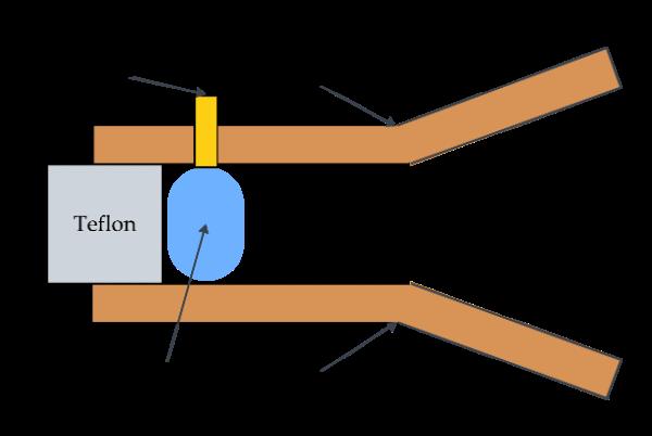
Fig. 2. Diagram of a rectangular flared electrode PPT geometry. The electrodes flare out at a 20° angle partway down the chamber after the ignition site. The ignition circuitry is not changed in any way from the rectangular geometry.

cause is upon the reliability of the thruster. It has been observed that an electrode angle greater than 20° has a negative impact on the reliability of the thruster. This increase in probability of misfire is due to the increased distance between electrodes, resulting in a diminished magnetic field between the electrodes, decreasing the present Lorentz force and thus accelerating plasma less. Beyond 20°, reliability continues to decrease with a 40° angle on both electrodes, resulting in an ignition failure rate beyond 80% (Li et al., 2021), practically rendering the thruster useless. This was also observed by Li. et al (2021), where it was concluded that the electrode angle is inversely proportional to the reliability of the thruster.

Despite the drawbacks previously mentioned, the flared electrode geometry has been shown to increase the efficiency and effectiveness of PPTs. Specifically, an angle of 20° was observed as increasing the efficiency of the thruster by 35% in reference to the frequency of discharge, thrust, and mass of propellant used per pulse and increasing exhaust exit velocity by 20% (Schönherr et al., 2010). Additionally, the 20° was observed as improving the thrust-to-power ratio per pulse (Arrington et al., 1997). These benefits can potentially mitigate the decrease in reliability as a result of electrode angle; however, in reality, this configuration and all other configurations of PPTs for that matter, are dependent upon variables beyond the scope of this paper. For example, electrode length has a large impact on the performance of the flared electrode geometry thruster. As was observed and tested by L. Arrington and N. Meckel (1997), a change in electrode length from 2.54 cm to 3.81 cm in the same configuration previously

Fig.

Thornburg

discussed, yielded increased efficiency but did not improve the power-to-thruster ratio. Thus, it is known that the length of the electrode after being angled does significantly impact the performance of the thruster, it is a subject beyond the scope of this review.

Co-axial Electrode Orientation

Among the 119 infants included in this study, 48% developed atopThere are two main types of coaxial geometries, both of which are pictured in figures 3 & 4. The main difference between these models is the extension of the anode through the center of the cylindrical chamber created by the cathode. In the annular configuration, the anode is a cylindrical rod, and it extends inside the chamber created by the cathode. The chosen fuel force surrounds the anode, filling the space between both electrodes. Ablation occurs inside the cavity of the cathode and in front of the anode electrode. The tip of the anode should not protrude beyond the surface of the fuel source and the length of the cathode cavity down which the plasma is accelerated should be of minimal. Alternatively, in the coaxial cavity geometry, the anode is located in the rear of the nozzle behind the fuel source. In this configuration, ablation occurs along the walls of the chamber along the surface of the fuel, with the resulting ions being accelerated through the cavity in the center of the cathode electrode.

In the coaxial geometry, it has been observed that the length of the cavity between the fuel source and the end of the cathode cylinder has a large influence upon the reliability of the thruster. Specifically, the overall lifetime of the thruster can be increased by shortening the cavity due to the decrease in the buildup of contamination along the electrode surface. Additionally, the cathode cavity can be flared out in a similar manner to the electrodes in the flared rectangular PPT geometry to further improve upon the lifetime of the thruster by further reducing contamination buildup by more effectively moving exhaust gas, resulting in an improved impulse bit. Consequently, the larger the angle becomes, the less reliable the thruster is, with angles at and above 60° significantly reducing the reliability of the thruster. As for the anode in the annular geometry, protrusion of the electrode beyond the surface of the fuel source changes the

geometry. The dashed line represents the axis of symmetry around which the nozzle revolves.

A Performance Review of Nozzle Geometries

characteristics of the system’s discharge and ignition, resulting in increased charring of the fuel source. (Aoyagi et al., 2024). As was also noted for the rectangular geometries, electrode size also has a large impact on the thruster’s performance. However, in the case of coaxial geometries, chamber diameter is also of similar importance. Increasing the length of the cavity has been shown to increase the ablated mass per pulse and thus improve the impulse of the thruster, while increasing the diameter of the cavity reduces the ablated mass per pulse (El-Hadeed et al., 2025). Additionally, widening the diameter of the cavity results in uneven ablation of the solid fuel surface, resulting in unstable future ablation (Fu et al., 2024).

Just as the size of the electrodes is important for the previously described reasons, their size also impacts the energy density of the thruster, which is an important characteristic of performance in coaxial geometries. An energy density under 0.11 J/mm^2 has been found to result in increased charring of fuel, while an energy density of 0.23 J/mm^2 and higher is necessary to maintain efficient operation for the duration of the thruster’s lifespan (Aoyagi et al., 2024).

Conclusions

The future of PPTs is largely dependent upon their implementation into the larger space industry.To this, it is necessary for PPT to continually be innovated and improved upon in order to be a practical choice for space missions. Nozzle geometry, one of the most impactful characteristics of a PPT, is largely ambiguous regarding what the optimal choice is. As it currently stands, each PPT geometry is comparatively unique from one another in its performance, meaning that each geometry is best applied in different scenarios. It currently appears that the coaxial geometry will grow to become commonplace in missions utilizing microsatellites due to the larger impulse and impulse bit provided by the geometry making them better for larger maneuvers. The higher thruster strength provided by this geometry however proves disadvantageous for missions in which PPTs are to be utilized for attitude control and station keeping.Thus meaning that the rectangular geometry, which possesses a comparatively lower

The dashed lines represent the axis of symmetry around which the nozzle revolves.

Fig. 3. Coaxial annular PPT

Fig. 4. Coaxial Cavity PPT Geometry.

impulse bit and high fuel efficiency, will remain a prime choice to missions in which the PPT is not the main source of thrust.

The iteration and innovation currently occurring in the PPT and electronic propulsion system field as a whole, has greatly advanced the field of alternative propulsion systems to liquid fuel combustion thrusters. However, the implementation of these thrusters into satellites and spacecraft is a severely under studied area of the expanding industry. Much of the research currently being done regarding PPTs has focused upon the characteristics of the thrusters themselves and not their ability to integrate into existing spacecraft. The greatest issue presented by this gap in knowledge is whether the current microsatellites are capable of supporting and operating a PPT for the mission duration. Since microsatellites can often only produce a limited supply of electricity due to constraints of solar panels, it is important to consider whether the power requirement of a PPT and critical spacecraft hardware is practical for a microsatellite to support. Though there are other major limitations that PPTs are currently inhibited by such as fuel inefficiency, late time ablation, slow moving exhaust gas, etc., this presents one of the largest gaps in knowledge regarding PPTs with there being little scientific literature regarding the topic. Thus it is imperative that an understanding of the relationship between electronic propulsion systems and microsatellites is built.

Nozzle geometry is an important field of study for electric propulsion systems as it explores the ways in which each unique PPT geometries excel. Akin to how certain liquid fuel combustion thrusters specialize in atmosphere versus in vacuum or are reusable versus single use, the different geometries of PPTs all serve uniquely different purposes due to their different characteristics. Thus not only is it important for PPT to continue to be innovated upon at large, but also for each individual geometry to be further specialized towards its niche.

Works Cited

Aoyagi, J. A., Yamada, M. Y., Tezuka, T. T., Watanabe, R. W., Otsuki, T. O., & Takeya, S. T. (2024). Series Development of Coaxial Pulsed Plasma Thruster From 1 J to 8 J, Journal of Electric Propulsion. https://doi.org/10.1007/s44205-025-00135-z

Arrington, L. A., Haag, T. H., Pencil, E. P. & Meckel, N. M. (1997). A Performance Comparison of Pulsed Plasma Thruster Electrode Configurations [Conference Presentation]. International Electric Propulsion Conference, Cleveland, Ohio.

El-Hadeed, M.M.A., Abdelkader, M.E., Diab, F.B. et al. Investigation of a coaxial pulsed plasma thruster by electrothermal discharge in Teflon propellant. CEAS Space J (2025). https:// doi.org/10.1007/s12567-025-00637-4

Fu, F. H., Wu, Z. W., Huang, T. H., Hu, T. H. & Zhang, S. Z. (2024). Influences of initial voltage and electrode size on propellant surface evolution in a coaxial pulsed plasma thruster, Acta Astronautica, 222, 573-585, https://doi.org/10.1016/j. actaastro.2024.06.032.

Kaseez, M. K., Khondenko, V. K. (2019). Hybrid Electric Propulsion System on the Basis of SPT and PPT [Conference Presentation]. International Electric Propulsion Conference, Vienna, Austria.

Li, Y. L., Dorn, K. D., Hsieh, H. H., Kuo, T. K., & Hsu, Y. H. (2021). Journal of Aeronautics, Astronautics and Aviation, 53 (3), 353 - 368. 10.6125/JoAAA.202109_53(3).02

Ling, W. L., Zhang, S. Z., Fu, H. F., Huang, M. H., Quansah, J. Q., Liu, X. L. & Wang, N. W. (2020). A Brief Review of Alternative Propellants and Requirements for Pulsed Plasma Thrusters in Micropropulsion Applications. Chinese Journal of Aeronautics, 33(12), 2999 - 3010. https://doi. org/10.1016/j.cja.2020.03.024

Schönherr, T. S. Nawaz, A. N., Lau, M. L., Petkow, D. P., & Herdrich, G. H. (2010). Review of Pulsed Plasma Thruster Development at IRS. JSASS Aerospace Tech. Japan, 8 (27), 11-16.

Woodruff, C. W., King, D. K., Burton, R. B.. & Carroll, D. C. (2019). Fiber-fed Pulsed Plasma Thruster (FPPT) for Small Satellites (Conference Presentation). University of Vienna, Vienna, Austria.

Yang, L. Y., Liu, Q. L., Zhao, X. Z., & Huang, Y. P. (2019). Analysis of Distributed Energy Release Characteristics in an Ablative Pulsed Plasma Thruster [Conference Presentation]. International Electric Propulsion Conference, Vienna, Austria.

RESEARCH & DISCOVERY

The Effects of Melatonin

Evie Tucker

Abstract

Melatonin is a hormone that regulates the sleep-wake cycle that most likely influences mood and behavior. This study helps explain how melatonin affects sleep quality and mood by asking individual participants to record their sleep patterns. Half the participants took the melatonin supplement orally each night and the other half did not. Using a daily mood assessment called the Profile of Mood States (POMS) scale, the participants logged their sleep patterns and mood changes. Results show that individuals who took melatonin had lower levels of anger, confusion, fatigue, and tension compared to non melatonin users (p < 0.05). Overall mood disturbance was reduced, while vigor and depression showed little to no change. Although this study had a small sample size and uncontrolled dosage of melatonin, the results suggest that melatonin improved mood and relaxation. This is because melatonin actively regulates the circadian rhythm. For future research, for more success using a larger sample size and controlled samples would better confirm the effects of melatonin.

Introduction

Do you ever wonder what makes you feel tired at the end of the day? Melatonin plays a significant role. Melatonin is a hormone produced by the pineal gland located in the brain, which regulates the circadian rhythm.The circadian rhythm contributes to the sleep-wake cycle. For melatonin to affect the signals in the brain it needs to interact with membrane MT1 and MT2 receptors and the intercellular proteins. (Musshoff et al., 2002).

Melatonin affects intracellular cyclic otherwise known ascAMP, cGMP and calcium levels. ascAMP is aspartic acid which transmits signals between neurons in the brain. cGMP is the cyclic monophosphate which is another messenger neuron that is mainly used by eukaryotic cells. It helps activate the protein kinases to help build the membrane peptides for the external cells in the brain. Intracellular cyclic is a messenger inside of the cell that signals the regulation process outside of the cell. Then these affect protein kinase C and the steroid hormones which help regulate protein G that signals other proteins. Tryptophan is a hormone that creates melatonin in the brain which is turned into serotonin that converts into an enzyme. The enzyme arylalkylamine-Nacetyl that is metabolized in the melatonin (Axelrod and Wurtman, 1968). Serotonin helps control your mood, movement, and sleep which regulates your sleep-wake cycle. Due to melatonin increasing the REM cycle which is when most dreams occur, most people have reported vivid dreams that often seem strange or unsettling. It is hypothesized that melatonin is related to a change in behavior while sleeping. This is due to the fact that melatonin is associated with darkness which causes you to become more tired. Due to serotonin levels changing the neurotransmitter helps reduce anxiety behaviors (Jean-Louis et al., 1998). With a better understanding of how melatonin affects the brain I conducted a similar experiment to the Lieberman study. It will follow the simple guidelines along with some alterations.

A study was conducted where fourteen participants between the ages of 18 and 45 were tested to see how melatonin affects

mood and performance. Before the study each participant was given a physical exam to see the differences with and without melatonin. These men were split into two groups, the first group was given melatonin and the second group was given a placebo. There were two sessions for this study to create a clean slate from the session before. During the sessions the participants received 240mg of melatonin or the placebo which was separated into three 80mg doses (Lieberman et al., 1984). I want to use this paper as a model for my presumed experiment which is finding out how melatonin is effective to teens’ mood patterns and sleep

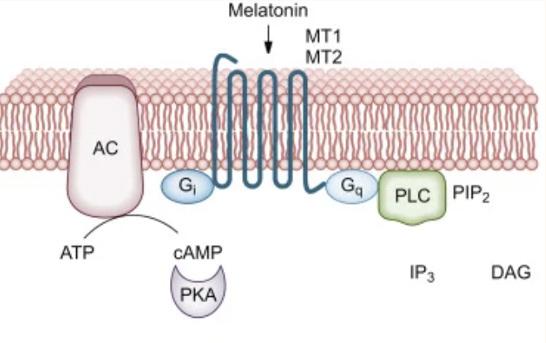
Fig. 1.The binding site for melatonin reacting to the receptor inside the pituitary gland. (Wang et al., 2005).

schedules.

The purpose of this study is to better understand how melatonin truly affects the brain when sleeping. If people take melatonin before going to sleep, then they will have better sleep quality and improved moods compared to people who do not take melatonin. Understanding how melatonin affects the brain is important because most times we take the pill without thinking twice about how it works. For this study a test will be conducted with participants who volunteer to take melatonin during a scheduled period of time. They will record their sleep patterns, what kinds of dreams they have, and the quality of their sleep. Then I will ask those who do not take melatonin to record their sleep patterns for two weeks. After the study is completed I hope to have a better understanding of how melatonin makes you tired, affects the quality of sleep, and changes how your brain works when you sleep; if you have more or less dreams how severe they are. If melatonin helps improve mood if it is taken before bed then why don’t more people take it?

Methods

For this experiment, I created a study similar to the Lieberman et al. (1984) study.

A google form was sent throughout the school that has a series of questions related to how melatonin affects your mood. To collect the results I used a POMS scale. In order to analyze my data I asked each participant to fill out the questions each day and send me screenshots of their results which were calculated in a spreadsheet.

After doing some extra research I found a specific test called the POMS, Profile of mood state. scale from Upenn and Stanford. It is a scale that has 65 questions which can be answered on a scale from; not at all, a little, moderately, quite a bit and, extremely. After all questions were filled out they would press the “analyze” button to obtain the TMD, total mood disturbance. Then they had to analyze the TMD number to determine their mood profile. (Shahid et al., 2012). This recorded the participant’s mood each morning (Mackenzie, 2001). This should be a reliable form of data capturing because many other studies have the POMS scale.

Another way to obtain the data would be through a series of surveys. The survey would ask about the quality of sleep to make sure I receive the same data from each participant. To analyze the data I created a bar graph with error bars to see outliers. Using AI we determined the best way to find differences between both independent groups. The Welches T-test was used which is a t-test that assumes both groups have equal variance and is best used when dealing with small sample sizes.

Results

In this study I have focused on how melatonin affects one’s mood. I used a variety of questions based on the POMS scale. The scale consists of five categories: anger, confusion, depression, fatigue, tension, and vigor.

Comparing both results of the control group (without melatonin) and experimental group (with melatonin) had slight differences, we can infer that the melatonin users had a much calmer Circadian Rhythm due to the melatonin receptors in the brain being activated. Using the POMS scale helps provide a more accurate form of results. The difference between taking

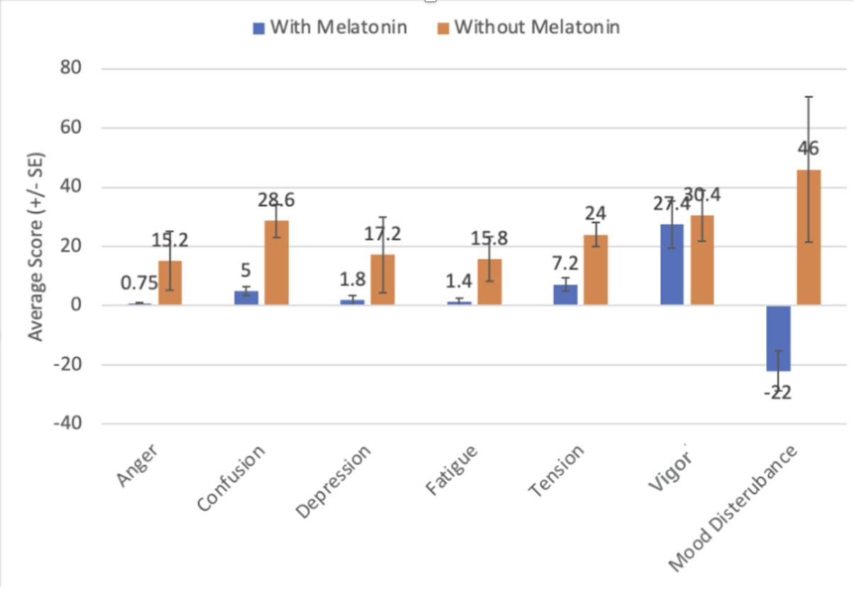
Fig. 2. Difference in mood disturbance between those who take melatonin and those who do not. Error bars represent standard error of the mean.

melatonin and not taking melatonin is prominent in this study. The graphs show with melatonin the brain can improve overall mood disturbance.

For melatonin administered subjects, melatonin lowered the amount of anger, confusion, fatigue, and tension (p<0.05; Welch’s t-test).. The mood disturbance shows more reliable results, showing how the melatonin group averaged -22.0 as a score. The negative number implies mood disturbance is very low. The nonmelatonin group averaged 46.0 making the difference significant as the (P < 0.0015). Vigor (energy) was a mood that was minimally impacted showing no significant difference with a score of (P > 0.7494). This suggests that the melatonin users felt less stressed and angry when taking melatonin before bed although minimal change in energy levels throughout the day with a difference of (P = 0.0528).

Discussion

Although there were only 12 participants in this study, six who take melatonin and six who don’t take melatonin, my hypothesis is supported that melatonin relaxes the brain.There was a significant improvement in all areas of the POMS study except for depression and vigour. The results show how melatonin can improve overall sleep quality resulting in a more stable mood.

Originally I planned to follow the Lieberman study. The study

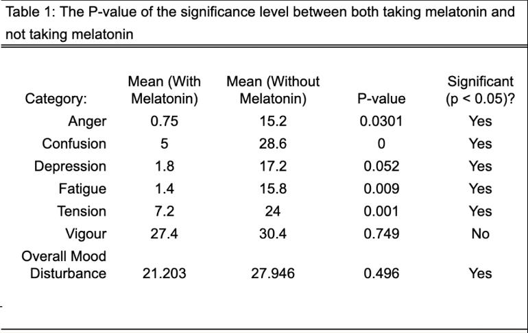
asked: (why) if they dream, if they wake up, and how well rested they are will they have mood stability? (Lieberman et al., 1984). However, their experiment followed strict rules which I was not able to replicate. In the Lieberman study there were a total of 14 male participants. I had 12 participants who were all teen girls. Although the participants were different, comparing the results was not easily obtainable between both studies due to the fact that I had limited resources. Similarly I was not able to control the time and amount of melatonin administered because this was an unmaintained study. I did not want to change people’s sleeping habits. This caused each participant to have uncontrolled outcomes causing my data to be skewed and unreliable. If I were to do this experiment again I would obtain more participants to solidify my hypothesis and show how beneficial melatonin is for overall mood health.

Works Cited

Axelrod, J., Wurtman, R.J., (1968). Photic and neural control of indoleamine metabolism in the rat pineal gland. Adv. Pharmacol. 6, 157–166.

Lieberman, H. R., Waldhauser, F., Garfield, G., Lynch, H. J., & Wurtman, R. J. (1984a). Effects of melatonin on human mood and performance. Brain Research, 323, 201-207.

Lieberman, H. R., Waldhauser, F., Garfield, G., Lynch, H. J., & Wurtman, R. J. (1984b). Melatonin receptors in rat hippocampus: molecular and functional investigations. Hippocampus 12, 165–173.

Mackenzie, B. (2001). Profile of Mood States (POMS). BrianMac Sports Coach. Retrieved [date you looked at it].

Musshoff, U., Riewenherm, D., Berger, E., Fauteck, J.D., Speckmann, E.J., 2002.

Jean-Louis, G., von Gizycki, H., & Zizi, F. (1998). Melatonin effects on sleep, mood, and cognition in elderly with mild cognitive impairment. Journal of Pineal Research, 25(3),177–183.

Shahid, Azmeh, et al., editors. Stanford Sleepiness Scale (SSS). STOP, THAT and One Hundred Other Sleep Scales, Springer, 2012.

Wang, L.M., Suthana, N.A., Chaudhury, D., Weaver, D.R., Colwell, C.S., 2005 Melatonin inhibits hippocampal long-term potentiation. Euro. J. Neurosci. 22, 2231–2237.

RESEARCH & DISCOVERY

Python-based Analytical Modelling for Waste Thermal Energy Recovery in Air Conditioner Systems

Parika Verma

Abstract

The hospitality sector, characterized by its substantial energy demands for space conditioning, presents a significant opportunity for waste heat recovery, particularly from air conditioning systems. This is especially pertinent in tropical climates where cooling loads are consistently high, leading to substantial thermal energy being rejected into the environment.

This study focuses on recuperating this waste thermal energy, via a compact plate-heat heat exchanger.Two machine learning models were used to analyse performance, offering a data-driven approach to optimise energy reuse and mitigate environmental impact.

This study found that plate-type heat exchangers recovered a substantial proportion of waste thermal energy from hotel air-conditioning systems, with recovery rates ranging from 65-82%, under realistic operating conditions. The integration of Python-based analytical modelling with LightGBM machine learning successfully predicted hourly condenser heat rejection and evaluated system performance dynamically across varying environmental and operational conditions. The results showed that waste heat recovery significantly improved overall HVAC energy efficiency, with annual system efficiency averaging 76.4% and estimated energy recovery reaching 480-620 MWh per year for a 300-room hotel. The modelling framework also identified the influence of key design parameters, including water flow rate, plate count, and pipe diameter, on heat exchanger effectiveness. Overall, the findings demonstrated that data-driven thermal analysis provided a practical, low-cost, and scalable approach for improving energy efficiency and reducing environmental impact in hospitality HVAC systems.

This research thus represents a critical step towards developing data-driven solutions for enhanced energy efficiency and environmental stewardship.

Introduction

The hospitality sector ranks among the most energy-intensive commercial industries, with air conditioning accounting for a dominant share of total energy consumption. In tropical and subtropical regions, hotels operate cooling systems nearly year-round, leading to continuous rejection of large quantities of low-grade thermal energy from condenser units. This rejected heat, while often overlooked, represents a stable and predictable energy source with significant recovery potential.

Plate-type heat exchangers (PHEs) are well suited for recovering condenser waste heat due to their compactness, high heat transfer coefficients, and effectiveness at low temperature differentials. Previous studies have demonstrated their applicability in industrial and domestic heat recovery contexts (Masoumpour, 2021). However, practical adoption in hotel HVAC systems remains limited. One key barrier is the difficulty of accurately estimating available waste heat under real operating conditions, which vary hourly with climate, occupancy, and system load.

Conventional approaches rely heavily on detailed simulations or experimental prototyping, both of which are costly and inflexible during early design stages. Recent advances in machine learning offer an alternative: data-driven prediction of system behaviour that can be coupled with first-principles thermal analysis.

This study proposes a hybrid framework that integrates machine learning-based condenser heat prediction with analytical plate heat exchanger modelling. The objective is to quantify recoverable waste heat, identify optimal design parameters, and

evaluate system efficiency under realistic, time-varying conditions. While the focus is on hotel air-conditioning systems, the methodology is broadly applicable to other commercial cooling applications.

Methods Modeling Framework

The modeling framework followed a two-stage structure approach in order to ensure both predictive accuracy and physical reliability. In the first stage, a machine learning model is developed to predict the hourly condenser heat rejection based on the environmental and operational inputs (ASHRAE Great energy Predictor III) (Kaggle, 2025). In the second stage these predictions are integrated with the heat exchanger theory (Serhat & Boskovic, 2020) to estimate the amount of the recoverable heat and the overall system efficiency. This combined approach allowed the analysis to move beyond assumptions by linking it to

real-world operating behavior with established thermal, dynamic relationships. All modeling was implemented in Python, which ensured low computational cost, reproducibility, and practicality for large-scale applications.

Machine learning model

The predictive model is based on a Light GBM (light gradient boosting machine) regression algorithm (Ke, 2017) selected due to its strong performance with large datasets and its ability to capture complex nonlinear relationships between variables. The model uses input features such as ambient conditions representing hotel HVAC systems and cooling load. The model performance is evaluated using Root Mean Squared Error (RMSE), where the initial model achieved an RMSE of 1.178, corresponding to an uncertainty of approximately 18%. After the hyperparameter optimization which helps the algorithm align design variables for best thermal performance, the RMSE improves to around 1.07, reducing uncertainty to approximately 7-8%.This level of accuracy is considered acceptable for preliminary engineering design and system sizing (Dubois,2021), demonstrating that the model can reliably predict condenser heat output under varying operating conditions.

Heat Exchanger Analysis

The predicted condenser heat rejection was then coupled with a compact plate-type heat exchanger model using the effectiveness-NTU method which is a direct approach for evaluating heat exchanger performance when the outlet temperatures are unknown, using the heat exchanger effectiveness and the Number of Transfer Units (NTU) (Subramanian,2019). This approach allowed for the estimation of actual heat recovery while accounting for realistic system constraints. Key parameters such as water mass flow rate, heat transfer surface area, number of plates, and pipe diameter are incorporated into the analysis. By evaluating these variables, the model calculates the hourly system effectiveness and recovered heat across an annual operating cycle. This integration ensures that the predicted performance reflects both the variability of the operating conditions and physical limitations of the heat exchanger.

Virtual design optimization

Once trained, the model was enabled for rapid design scenarios through virtual optimization. By systematically varying parameters such as flow rate, plate count, and pipe diameter, the framework performed a “what-if” analysis that stimulated a wide range of configurations.This effectively created a computational test bench, allowing the performance trends and optimal design regions to be identified without the need for physical experimentation. As a result, the methodology not only predicted the system behavior but also supported design decision- making. Highlighting the practicality of using a LightGBM based approach for efficiency and scalable optimization.

Results

The results obtained from the LightGBM model demonstrate that the condenser heat availability remains consistently sufficient to support effective heat recovery under a wide range of operating conditions.The trained model predicts that, when coupled with an

1. Predicted condenser waste heat generation as a function of outdoor temperature

Fig. 2. Optimisation analysis showing the relationship between pressure drop and recovered heat for different water flow rates, highlighting optimal design zone.

appropriately designed plate heat exchanger (PHE), approximately 65% to 82% of the rejected heat can be recovered successfully under realistic system behavior. As illustrated in Figure 1, the availability of condenser waste heat increases with rising outdoor temperatures.

The sensitivity analysis was conducted through virtual optimization, and further clarified the influence of key design parameters on system performance. Increasing the water flow rate through the heat exchanger improved the predicted heat recovery up to a certain threshold; however, beyond this point the diminishing returns are observed. This trend was reflected in the optimization results shown in Figure 2, where the recovered heat increases with pressure drop (which is associated with higher flow rates) until reaching an optimal design region.

Similarly, increasing the number of plates significantly improved the heat exchanger effectiveness by expanding the available heat transfer surface area, where greater surface area corresponds to higher overall recovery. In contrast, pipe diameter presents a more complex trade-off. While larger diameters may improve thermal performance by reducing flow resistance and enhancing heat transfer they also increase system-level energy losses due to

Fig.

Fig. 3. Heatmap of predicted waste heat recovery as a function of ambient temperature and time of day, indicating peak recovery during afternoon hours and higher temperature ranges.

higher fluid circulation which is demanded and associated with frictional losses within the piping network.

As a result, optimization was required to balance these competing effects. The results indicate that no singular parameter independently maximized the system performance; instead, an optimal level exists where the heat recovery is maximized while minimizing the energy losses.

The daily distribution of recoverable condenser heat is where its state remained relatively stable throughout the operating cycle but increased slightly during afternoon hours. This trend aligns with higher cooling loads and elevated ambient temperatures during these periods.

The model predictions also vary with ambient temperature conditions. The system achieved efficiencies of approximately 80% to 85% when outdoor temperatures exceeded 28°C, as shown in Figure 3. The recovery occurred during afternoon periods when temperature surpassed 30°C, reflecting a stronger thermal gradient and increased heat recovery potential. And in mild conditions, predicted efficiency ranged from 60% to 70%. The annual average efficiency was calculated at 76.4%. (800 MWh (Q available) 611.2 MWh(Q recovered), n=611.2/800*100=76.4%)

For a representative large-scale application such as a 300 room

Fig. 4. Annual recovered energy from condenser waste heat across months, showing an average recovery of approximately 580 MWh per year.

Fig. 5. Plate heat exchanger’s effectiveness comparison to NTU (Number of transfer units) [showing how powerful/ capable the heat exchanger is at transferring heat] (Sciencedirect, 2024)

hotel, the total annual heat recovery was estimated to range between 482 and 620 MWh, (580 MWh shown in Figure 4) corresponding to approximately 18% to 22% of total cooling energy consumption.

The relationship between the exchanger performance and theoretical effectiveness is illustrated in Figure 5, which compares plate heat exchanger (PHE) effectiveness with NTU (Number of transfer Units), which is a dimensionless parameter used in heat exchanger analysis to show how effectively heat exchanger can transfer heat relative to its size and flow conditions. As shown, the theoretical curve follows a non linear trend, where effectiveness rapidly increases at lower NTU values and gradually begins to plateau, reflecting the returns at higher transfer units. The hotel data points generally follow this same trend, supporting the validity of the modelling approach, although they appear slightly higher than the theoretical predictions, likely due to some real-world operating conditions such as stronger temperature gradients or flow variations not fully captured in the model. This alignment confirms that the effectiveness-NTU method provides a reliable representation of system behavior, while also reinforcing that increasing NTU improves performance only up to an optimal range and beyond this the gains become marginal, highlighting the need for careful design optimization.

Discussion

This study set out to address the research question: How well can a plate-type heat exchanger recover waste heat from hotel air conditioners? The results confirm that waste heat recovery from hotel air-conditioning systems is not only feasible but also highly effective, with 65-82% of condenser heat successfully recuperated under realistic operating conditions. This confirms that the plate-heat type exchangers are well suited for this application, particularly when system behavior is evaluated, rather than through static assumptions.

The objective was achieved through the development of a hybrid modelling framework by integrating machine learning with established thermodynamic models. By using a LightGBM model to predict hourly condenser heat rejection and coupling it with

Verma Python-based Analytical Modelling for Waste Thermal Energy

effectiveness-NTU analysis, the study provides a detailed and time-resolved assessment of system performance. This approach overcomes the limitations of conventional simulation based methods, which are often data intensive and less adaptable during early-stage design.

Unlike static design calculations, the proposed framework captures hour-by-hour variability in system performance, which provides a more realistic assessment of long-term energy recovery. For example, the results showed clear fluctuations in heat recovery potential throughout the day, with peak recovery occurring during periods of highest cooling demand and reduced performance during the off-peak hours. This variation highlights the importance of the dynamic modelling, as static approaches would overestimate the performance by assuming constant operating conditions. By capturing these variations, the model provides more accurate estimates of cumulative energy savings over time.

Importantly, key variables including the time of year, water flow rate, and plate number play a critical role in determining performance and were implicitly optimized within the modelling framework. The framework is scalable, efficient, and suitable for feasibility analysis in the early stage, making it easier to adopt it in real life usage in commercial buildings without requiring extensive resources or physical prototyping. This lowers the barrier to adoption and supports the broader implementation of waste heat recovery strategies in the hospitality sector. This is particularly important as even during summer time when space heating demand is low, hotels have continuous demand for domestic hot water for guest use, laundry services, kitchens and pools. Recovered heat can therefore be directed to meet these loads, reducing reliance on conventional water heating systems and lowering overall energy consumption and operating costs.

However, several sources of error should be acknowledged. The accuracy of the LightGBM predictions depends heavily on the quality and representativeness of the data; and any missing data, bias and fluctuations during different seasons can affect model reliability as here we have modelled it based on climates in North India. Measurement errors in the input variables including temperature, flow rates and power consumptions can also affect results.Further assumptions were necessary to make the model traceable (eg. minor heat losses to the surroundings or fouling effects).

In the future, further development could focus on improving model accuracy through expanded datasets, as well as integrating real time building management system data for live optimization. Future work may also explore economic analysis in a greater depth, including lifecycle cost modelling and the payback periods alongside the experimental validation of the proposed system. Overall, the study demonstrates that combining machine learning with thermodynamic analysis provides a powerful and practical pathway for enhancing energy efficiency and sustainability in hotel HVAC systems. This approach is consistent with a growing body of research showing that data driven methods can significantly enhance heat recovery and energy system optimisation. For instance, prior studies in the field of HVAC engineering and energy systems engineering have reported heat recovery efficiencies typically ranging between 50-75% (Lamrani, 2024), when using conventional modelling or steady-state assumptions, particularly

in applications involving waste heat recovery from air-conditioning systems. In comparison, the 65-82% recovery achieved in this study demonstrates as not only competitive but in many cases even improved performance, particularly due to the incorporation of time-resolved system behavior.

Unlike earlier works that rely heavily on static or simulationbased approaches, this study advances the field by demonstrating how hybrid frameworks integrating machine learning models such as LightGBM with established thermodynamic methods like effectiveness-NTU analysis can capture transient variations with greater accuracy and lower computational cost. This contributes to the growing shift toward data-driven modelling in building energy research, where adaptability and scalability are increasingly prioritised.

Furthermore, this work extends current understanding by highlighting the importance of temporal variability in heat recovery potential, which is an aspect which is often overlooked in traditional analyses. By quantifying how performance fluctuates throughout the day and across operating conditions, the study provides deeper insight into realistic system behavior and longterm energy savings. This not only supports existing findings but also refines them by demonstrating that dynamic modelling can prevent overestimation of performance, thereby improving the reliability of the feasibility assessments.

Works Cited

ASHRAE - Great Energy Predictor III.” Kaggle.com, www.kaggle. com/competitions/ashrae-energy-prediction/data.

Masoumpour, Babak, et al. “Performance Evaluation of a Shell and Tube Heat Exchanger with Recovery of Mass Flow Rate.” Journal of the Taiwan Institute of Chemical Engineers, vol. 123, 1 June 2021, pp. 153–165, reader.elsevier. com/reader/sd/pii/S1876107021002819?token=4EEC6578441E1A453906E93D5DF162736DB96724DD74 26886F8E4CC470A53BD4D8445E546AB091A21951E41493C8435B&originRegion=eu-west-1&originCreation=20221122034756, https://doi.org/10.1016/j. jtice.2021.05.022. Accessed 22 Nov. 2022.

Dubois, Anne Migan, et al. “Estimation of the Uncertainty due to Each Step of Simulating the Photovoltaic Conversion under Real Operating Conditions.” International Journal of Photoenergy, vol. 2021, no. 1, 15 Oct. 2021, pp. 1–14, www.researchgate.net/publication/355330683_Estimation_of_the_Uncertainty_due_to_Each_Step_of_Simulating_the_Photovoltaic_Conversion_under_Real_Operating_Conditions, https://doi.org/10.1155/2021/4228658.

Bilal Lamrani, . “Comprehensive Analysis of Waste Heat Recovery and Thermal Energy Storage Integration in Air Conditioning Systems.” Energy Conversion and Management X, 1 Sept. 2024, pp. 100708–100708, https://doi.org/10.1016/j. ecmx.2024.100708.

Subramanian, M. Heat Transfer Heat Exchangers -Effectiveness-NTU Method. 2019

Beyeni , Serhat, and Sanja Boskovic. “1.5: Heat Exchangers.” Workforce LibreTexts, 28 Nov. 2020,workforce.libretexts. org/Bookshelves/HVAC_and_Power_Plant_Operations/ Sim_Labs_for_Thermodynamics_and_Thermal_Power_ Plant_Simulator_(Beyenir_and_Boskovic)/01%3A_Sim_

Verma Python-based Analytical Modelling for Waste Thermal Energy Labs/1.05%3A_Heat_Exchangers.

Ke, Guolin. LightGBM: A Highly Efficient Gradient Boosting Decision Tree. 2017

“Number of Transfer Unit - an Overview | ScienceDirect Topics.” Www.sciencedirect.com, www.sciencedirect.com/topics/ engineering/number-of-transfer-unit.

RESEARCH & DISCOVERY

Lost in Translation? Evaluating AI and Human Translation in Diplomatic Communication

Sivan Yosha

Abstract

This study investigates how artificial intelligence translation systems alter diplomatic language and whether those changes influence reader interpretation. Focusing on a speech delivered originally in French at the 30th Ambassador’s Conference in Paris, the study compares an AI-generated English translation by the platform Kimi with a sworn human translation. A total of 45 participants were randomly assigned to read one version and evaluate it across nine categories, including formality, clarity, naturalness, and perceived speaker confidence. Statistical analysis using one-way ANOVA showed that while the human translation received consistently higher ratings across all categories, the differences were not statistically significant, though confidence in understanding approached significance. These findings suggest that AI translation can replicate formal aspects of diplomatic language but may reduce clarity and nuance, affecting reader comprehension. Overall, the study highlights that even subtle shifts in translation can drastically influence interpretation in high stakes settings, emphasizing the continued importance of human oversight in communication contexts such as diplomacy.

Introduction

Words and language are the primary vehicles of diplomacy. They carry intention, tone, and the delicate balance of international relationships. Diplomatic language often operates through subtle implications, metaphors, and even restraint, qualities that are essential for cooperation in some of the globe’s most important conversations. As artificial intelligence increasingly mediates communication between nations, translation has become not only a linguistic task but also an ethical one. Machine translation systems, while efficient and widely used, frequently struggle to reproduce the layered and ambiguous qualities of human speech (Jiang, 2024; Lu, 2025). These limitations raise important questions about what is lost when human translators, who have been trained to understand culture and context, are replaced by algorithms.

Recent research highlights both the potential and the risks of relying solely on technology for translation. Large language models have made rapid progress in recent years in producing fluent, natural-sounding text. But, they often simplify complex ideas that smooth over the tone that gives diplomatic language its subtlety (Di Martino & Ford, 2024; Bano et al., 2023). Chaudhri and Zowghi (2023), for example, found that generative AI tends to normalize political expressions across cultures, softening phrases or turning cautious diplomatic statements into more assertive ones. These are alterations that can shift perceived intent drastically in crossnational and cross-lingual conversations. Similarly, He et al. (2020) demonstrated that machine translation outputs frequently violate referential transparency, meaning ideas or references become inconsistent when translated back and forth.These inconsistencies suggest that subtle meanings risk distortion when processed through AI systems.

These findings show that AI translation can and does unintentionally reshape a message rather than merely transfer it directly. As translation becomes faster and more automated, diplomacy itself begins to shift, valuing efficiency and precision over empathy and cultural sensitivity (Akhmedov, 2024). In fields where each word carries political or symbolic weight, such as SinoAmerican relations, even small mistranslations can alter meaning

or weaken expressions of shared understanding (Semenov & Tsvyk, 2021). Similar patterns appear in other cross-cultural communication in tourism and healthcare, where AI translations can unintentionally change persuasion, tone, or emotional impact (Chen & Lin, 2025; Wong et al., 2025). While AI can positively bridge linguistic gaps, it may also reshape the very message it translates, adjusting how the meaning survives or changes across translation systems.

While previous research looked at AI platforms in general, I would like to focus on how specific translation platforms alter diplomatic language in ways that may not be immediately obvious, yet still influence how readers interpret political tone and intent. While past studies tend to concentrate on technical accuracy or isolated translation errors, this research will look at the more subtle shifts that can accumulate across commonly used platforms. By examining the commonly used AI tool Kimi that renders the same set of diplomatic phrases, the project highlights the patterns and inconsistencies that emerge when language meant to be careful and strategic is filtered through different systems. What makes this study unique is its emphasis on perception; instead of only analyzing the translations themselves, it also considers how readers respond to them, revealing which alterations are noticeable, which go undetected, and how those shifts might

affect understanding. This research explores the balance between innovation and understanding, how the growing use of AI in communication might enhance connection across languages, but also raises the stakes of human diplomacy. The hypothesis of this study is that human translators will outperform AI translation systems in persevering diplomatic tone, cultural nuance, and intended political meaning across languages.

Methods

This project used a two-part approach to study how AI translation platforms change diplomatic language and how these changes influence reader interpretation. In the first part of the study, I collected an excerpt from a speech that was dense with diplomatic phrases. The paragraphs I selected are from the 30th Ambassador’s Conference in Paris, delivered originally in French by Jean-Noël Barrot (2025). The speech as a whole included themes of state sovereignty, international law, conflict resolution, and appeals to the international community. I then entered the excerpt into a major AI translation tool: Kimi. To incorporate a control, I also found a sworn human translation, which served as a baseline for comparison. Forty-five participants (23 in the human translated group and 22 in the AI translated group) took one of the two blind surveys on Google Forms, where they read the excerpt that included the passage translated by either a human or Kimi, without being told which was which. For each statement, they rated tone, formality, clarity, and intent. Their responses showed whether the differences created by AI translation are noticeable to readers and which types of shifts are most likely to affect interpretation. I analyzed the survey results with an Analysis of Variance (ANOVA) to compare responses to the human translation versus the AI translations. The open-ended survey questions I read and interpreted to identify recurring themes in how readers interpret diplomatic statements. Each translated phrase was compared to the human English translation version to evaluate changes in tone, naturalness, clarity, politeness, formality, persuasiveness, and respectfulness. These are all elements that matter significantly in diplomatic communication.

The method’s design allowed this study to show not only how AI systems alter diplomatic language, but also how those changes impact the way people understand the meaning.

Results

A total of 45 participants completed the survey, with 22 in the AI-translated text group and 23 in the human-translated text group. Participants rated each passage on a scale from 1 to 10 across nine categories: formality, politeness, naturalness, clarity, perceived speaker confidence, persuasiveness, confidence in understanding, emotional tone, and respectfulness.

As shown in Figure 1 and Table 1, the AI translation scored highest in formality (M=8.41) and perceived speaker confidence (M=8.23), with moderate ratings for respectfulness (M=7.32), politeness (M=6.82), and persuasiveness (M=6.77). Lower ratings appeared for naturalness (M=4.64), emotional tone (M=4.64), clarity (M=5.05), and confidence in understanding (M=5.82), suggesting the text was formal but somewhat difficult for participants to understand and interpret.

The human translation as seen in Figure 1 and Table 2, followed a similar pattern but with consistently higher ratings. Highest scores

were in formality (M=8.87) and perceived speaker confidence (M=8.57), followed by respectfulness (M=7.91). Naturalness (M=5.27), clarity (M=5.64), and emotional tone (M=5.18) were also rated higher than the AI translation, indicating greater ease of comprehension. Direct comparison in Figure 1 shows the human translation rated higher across all nine categories, with the largest difference in confidence in understanding (M=6.91 versus 5.82). Moderate differences were observed in clarity and naturalness, and smaller differences in politeness, persuasiveness, and perceived speaker confidence.

To evaluate the differences between the two groups statistically, a one-way ANOVA was conducted across translation types for each category using Gemini AI. Consistent with the descriptive trends, the overall effect of translation type was not statistically significant across most categories (p>0.05), indicating that variation within participant responses was relatively large compared to differences between AI and human translations. The largest observed difference occurred in confidence in understanding the speaker’s main point, which approached the conventional significance level, while other categories showed smaller differences.

Post hoc comparisons, also conducted using Gemini AI, did not reveal statistically significant differences after adjusting for multiple comparisons (p>.05), reinforcing that although human translations were consistently rated higher, these differences were

Fig. 1. Comparison of average ratings between AItranslated and human-translated passages across nine categories. Ratings are based on participant responses using a 1-10 scale. The error bars in the graph represent the standard error.

not strong enough to be considered statistically significant. The difference in confidence in understanding the speaker’s main point approached the significance threshold, suggesting a potential trend that participants found the human translation easier to interpret. While this value is very close to the commonly used 0.05 cutoff, this threshold is arbitrary, and the result could mean possible significance.

Discussion

This study aimed to determine whether AI translation changed diplomatic language in ways that affected how readers interpreted tone and intent, and whether, in the long term, it could replace human translators. Overall, the hypothesis was only partially supported by this study. While the human translation was rated higher across all nine categories, these differences were not statistically significant at the typical level (p >0.05). However, the consistent pattern in the data, along with the near significant result for confidence in understanding, suggested that translation type may still have influenced reader interpretation in important, but subtle, ways. Even without statistical significance, the trends in the data were important. In every category, the human translation received higher average ratings, especially in clarity, naturalness, and confidence in understanding. These are all areas closely tied to how easily a reader can interpret meaning. In contrast, the AI translation performed well in formality and perceived speaker confidence but scored lower in categories related to comprehension and tone. These lower scores suggested that while AI was able to replicate the structure of diplomatic language, it may have struggled to preserve the nuance that made it easier to understand. The gap in confidence in understanding supported the idea that AI-translated text may have glossed over some of the subtleties that are crucial for deep understanding.

Although the statistical tests did not show significance, it is important to recognize that the 0.05 cutoff is somewhat arbitrary (Murtaugh, 2014). Results that approach this threshold could still point to meaningful patterns, especially in studies like this one with a small sample size. In this case, the near significant result for confidence in understanding suggested that with more participants or different conditions, a clearer difference might have appeared. Because of this, the lack of statistical significance did not necessarily mean that there was no effect, but it was not strong enough to be confirmed by this study. Several limitations could have influenced the results. One possibility is that participants did not have exposure to diplomatic language and, therefore, were unable to understand the subtleties of the excerpt. Which may have made it harder for them to distinguish between the two translations. In addition, the variation in responses suggested that individual interpretation played a large role. The sample size was relatively small (n=45), which reduced statistical power. A large portion of participants likely skimmed the text, which would result in an inability to notice the subtleties of the passage. Additionally, only one passage was used, so the results may not apply to all types of diplomatic language. Despite these limitations, it is still possible that this study contributed to the broader understanding of AI translation, particularly in diplomatic settings. Unlike many previous studies that focused primarily on technical accuracy, this research examines how translations were actually perceived by readers

largely unfamiliar with diplomatic language.The findings supported existing research suggesting that AI tends to simplify or standardize complex language, potentially reducing nuance. This study showed that these shifts not only affected the translations themselves but also how readers interpreted meaning. These results highlight the importance of reader perception, suggesting that even subtle changes could influence understanding and have an impact in real world contexts. At the same time, AI could have value in the future world of diplomacy. It could be useful in situations for efficiency and accessibility, particularly in moments that require quick communications, while still being supplemented by human translators.

Future research could expand on these results by using a larger sample size, including participants with more experience in language or international relations, and testing multiple passages and translation tools. It would also be useful to analyze open ended responses more deeply to better understand how readers interpret subtle differences.

While this study did not find statistically significant differences, the consistent trends suggested that AI and human translators were not perceived in exactly the same way. In particular, differences in clarity and confidence in understanding pointed to the possibility that AI translation might subtly affect how meaning is interpreted. As AI becomes more widely used in global communication, these small differences may become increasingly important.

Works Cited

Akhmedov, S. S. (2024). The impact of technology on diplomatic translation: Balancing innovation and human expertise. International Conference on Economics, Finance, Banking and Management, 182–186. https://econfseries.com/index. php/6/article/view/159?utm_source

Bano, M., Chaudhri, Z., & Zowghi, D. (2023). The role of generative AI in global diplomatic practices: A strategic framework. arXiv. https://arxiv.org/abs/2401.05415

Barrot, J.-N. (2025, 7 janvier). Discours de Jean-Noël Barrot, ministre de l’Europe et des Affaires étrangères, 7 janvier 2025. Ministère de l’Europe et des Affaires étrangères. https:// www.diplomatie.gouv.fr/fr/le-ministere-et-son-reseau/ actualites-du-ministere/30e-edition-de-la-conference-desambassadrices-et-des-ambassadeurs-6-7-janvier/article/ discours-de-jean-noel-barrot-ministre-de-l-europe-et-desaffaires-etrangeres-07?utm

Chen, S., & Lin, Y. (2025). A multidimensional comparison of ChatGPT, Google Translate, and DeepL in Chinese tourism texts translation: Fidelity, fluency, cultural sensitivity, and persuasiveness. Frontiers in Artificial Intelligence, 8, Article 1619489. https://www.frontiersin.org/journals/artificial-intelligence/articles/10.3389/frai.2025.1619489/full Di Martino, L., & Ford, H. (2024). Navigating uncertainty: Public diplomacy vs. AI. Place Branding and Public Diplomacy, 20(1), 350–354. https://link.springer.com/article/10.1057/ s41254-024-00330-z

He, P., Meister, C., & Su, Z. (2020). Testing machine translation via referential transparency. Proceedings of the 43rd International Conference on Software Engineering (ICSE), 410–422. https://ieeexplore.ieee.org/document/9402040 Jiang, X. (2024). A comparative analysis of human translation

and machine translation in diplomatic languages under the theory of functional equivalence: A case study of the US-China high-level strategic dialogue in 2021. Academic Journal of Science and Technology, 11(2), 219–222. https:// drpress.org/ojs/index.php/ajst/article/view/22374/21919

Lu, D. (2025). Translation quality of Chinese diplomatic discourse by NMT and LLMs based on multidimensional quality metrics. Journal of Theory and Practice in Linguistics, 2(5), 1–10. https://woodyinternational.com/index.php/jtpl/article/view/296/259

Semenov, A., & Tsvyk, A. (2021). The approach to the Chinese diplomatic discourse. Fudan Journal of the Humanities and Social Sciences, 14(4), 565–586. https://link.springer.com/ article/10.1007/s40647-021-00321-x

Wong, B. L. H., Aslanyan, G., Panichkriangkrai, W., Leite, R. B., Mahmood, J., & Nordström, A. (2025). From algorithms to negotiations: Why health diplomacy must adapt. PLOS Global Public Health, 5(4), e0004488. https://journals. plos.org/globalpublichealth/article?id=10.1371/journal. pgph.0004488

Yan, Z. (2024). The art of diplomatic discourse: Exploring the role of translation in international relations. International Journal of Frontiers in Sociology, 6(1), 6–11. https://francis-press.com/papers/14663

RESEARCH & DISCOVERY

Hypermobile Ehlers-Danlos Syndrome and the Correlation Between POTS and Reproductive Issues

Evalyn Zanibbi

Abstract

Hypermobile Ehlers-Danlos Syndrome (hEDS) is a connective tissue disorder that has been increasingly studied in relation to Postural Orthostatic Tachycardia (POTS), a form of orthostatic intolerance, an autonomic nervous system disorder that is characterized by increased heart rate causing dizziness, fatigue, nausea, and many other symptoms. Although the relationship between POTS and EDS remains unclear, this study is aimed to investigate the potential correlations between hEDS, POTS, and reproductive disorders. Data was collected from 18 participants through an online survey. Results showed no statistically significant correlation between hEDS, POTS, and reproductive disorders since p-val was 0.28 (p -val needed to be < 0.05 to be statistically significant). Similarly, no significant genetic association was identified through reported family history. Despite the lack of statistical significance, descriptive trends indicated that a notable portion of participants experienced all three conditions concurrently. Limitations of the study include a small sample size and potential variability in diagnostic criteria and participant interpretation. Further research with a larger and more diverse population is necessary to better understand these potential relationships.

Introduction

Connective tissue disorders were first recognized in the mid-20th century, although in the past couple of decades there has been an increase in understanding of one specific type: Ehlers-Danlos Syndrome. Ehlers-Danlos Syndrome, also known as EDS, has 13 different recognized subtypes (Malfait et al., 2017). Hypermobile Ehlers-Danlos Syndrome (hEDS) is the most common type of EDS, and represents about 90% of EDS cases. According to Mao, Jau-Ren, and Bristow (2001), EDS is a hereditary connective tissue disorder caused by abnormalities involving collagen and other extracellular matrix proteins that affect the strength and structure of connective tissues throughout the body. hEDS is characterized by generalized joint hypermobility, chronic musculoskeletal pain, autonomic dysfunction, fatigue, skin abnormalities such as soft, velvety skin, stretchy skin, or stretch marks all over the body that also bruises easily (Kurcharik et al., 2019).

In addition to the physical symptoms, individuals with hEDS often experience psychiatric and psychological complications, including anxiety, depression, and increased emotional distress, which may be linked to chronic pain, autonomic dysfunction, and the challenges of living with a chronic illness (Bulbena et al., 2017). However, there have been some studies that have found a correlation between EDS and another disorder, Postural Orthostatic Tachycardia Syndrome (POTS). POTS is an autonomic nervous system disease that is characterized by an excessive increase in heart rate when standing and is a specific type of Orthostatic Intolerance (Fedorowski, 2018). Orthostatic Intolerance is a broader condition that is characterized by increased heart rate when standing up, but is not specific in how much the heart rate changes, unlike POTS, which is characterized by an increase in heart rate of at least 30 beats per minute when standing (Fedorowski, 2018). The first reported association between EDS and orthostatic intolerance (including POTS) was described by Rowe et al. (1999). The links between POTS and EDS is still not fully understood, since POTS is mainly associated with autonomic nervous systems, while EDS is a connective tissue disorder. However, Kurcharik et al. (2019) was looking

for a correlation between hEDS, POTS, and Mast Cell Activation Syndrome (MCAS), but found that there was not a statistically significant correlation between hEDS and POTS.The authors state this was due to the fact that the sources used for this paper were methodologically limited since it relied on outdated or inconsistent criteria for diagnosing hEDS (Kurcharik et al., 2019). In contrast, in a study done in 2015 (Grigoriou et al., 2015) regarding orthopedic considerations, reported a significant association between EDS and POTS based on retrospective clinical data. In a review of 109 patients that were evaluated, 39 patients had POTS, and 7 of those (about 18%) had EDS. This is considered to be significantly higher than the estimated prevalence of EDS in the general population (around 0.02% of the population). Among the 70 patients without POTS, only three patients had EDS. The odds of having EDS were about five times higher in patients who had POTS than in autonomic patients without POTS. It is also important to note that patients diagnosed with EDS are typically females when they are in their 40’s or older, and people with POTS are mainly females with a mean age of 30 years old (Grigoriou et al., 2015).

Additionally, I personally have observed an apparent correlation between EDS, POTS, and certain reproductive

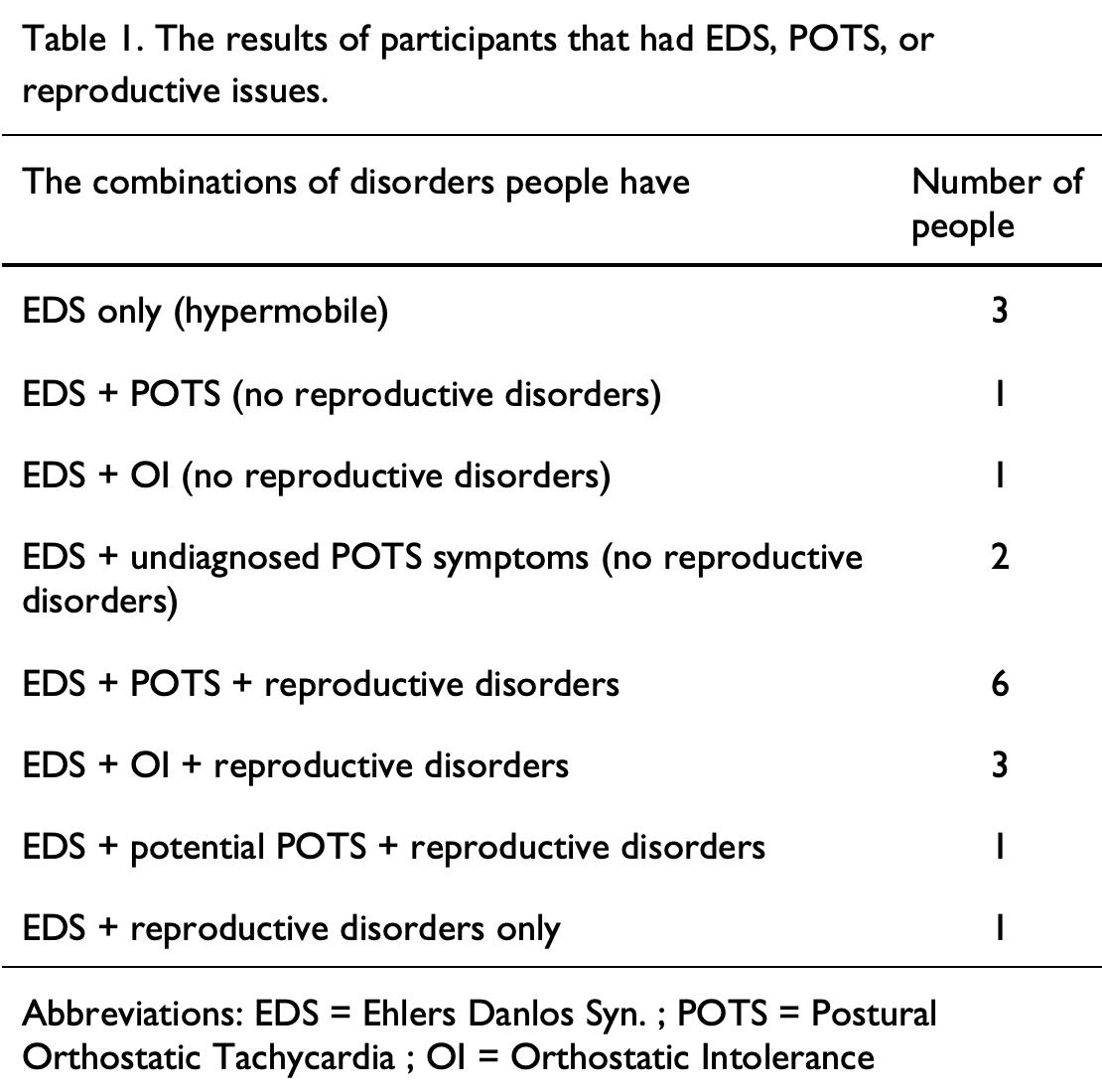
disorders. I am specifically trying to find any correlation with either Endometriosis, Adenomyosis, and polycystic ovary syndrome (PCOS). Endometriosis and adenomyosis are closely related disorders, both having the issue of endometrial tissue from the uterus growing in places it should not, as well as infertility issues, and problems with heavy bleeding or cramping during menstruation; this can potentially be dangerous and may cause additional issues. The main difference between these two reproductive disorders has to do with where the endometrial tissue grows. Endometriosis deals with the endometrial tissue growing and spreading outside of the uterus, which can lead to the tissue growing on organs such as the ovaries, fallopian tubes, pelvic peritoneum, or even organs such as the heart or brain in rare cases. For endometriosis you also run the risk of damaging the organs that the endometrial tissue may grow on in the worst cases. In contrast, adenomyosis has the growth of endometrial tissue growing within the muscular wall of the uterus (Bulun, 2023). PCOS is the most common endocrinologic condition in people born with a uterus and estimated to affect 8% to 13% of people with uteruses. Common symptoms of PCOS include irregular or absent periods, acne due to the excess androgen hormones, and excess hair growth around the back, chest, and face (Hoeger, 2021). The main purpose of this study is to see if there is a correlation either between specifically hEDS, POTS, and any of these reproductive issues as well as to examine the relationship between these conditions.

Methods

For this study I was looking for a correlation between specifically hEDS, POTS, and Endometriosis, Adenomyosis, or PCOS. I used certain social media platforms such as Discord to try and get substantial numbers of participants. This specific research study focused on people that were assigned female at birth, and the only main criteria for participation in this study is the subject had to have a diagnosis of EDS as well as either currently have or had

a uterus. A google form was used in order to get the information needed (https://forms.gle/n9Rh3D6MryZbxvfB9). Specific questions that were asked were the age of diagnosis of EDS and which subtype, as well as if they were diagnosed with POTS, and if they were diagnosed with either Endometriosis, Adenomyosis, or PCOS. I also collected data regarding if the participant had Orthostatic Intolerance (OI) since POTS is just a specific type of OI.There were also questions regarding if there were reproductive disorders that I did not take into consideration since I only went with the most common ones. Using this information, I was able to use statistical analysis to analyze all of the variables. I was also able to determine the difference in the probability of getting just one of the other disorders with hEDS. The goodness of fit chisquared statistical test was specifically used to examine bivariate associations between diagnostic categories between hEDS with a POTS diagnoses and hEDS with reproductive conditions. To help with the statistical analysis, there were also questions regarding certain family members, such as maternal parents and female siblings to see if there was a correlation with family members also having these disorders.

Results

The Chi Square test showed no significant effect between EDS, POTS, and reproductive disorders (Chi-Square; p-value > 0.05). The test also saw no significant effect between these disorders being genetically related as of right now. Regarding Table 1, out of the 18 participants, six had a combination of EDS, POTS, and some sort of reproductive disorder. Testing did not show this because there are very few family members who were diagnosed with EDS, being only three people, however there are five currently

looking into a diagnosis. But as stated before, hypermobile EDS has been shown to be hereditary (Malfait et al., 2017; Byers et al., 2017).This disorder just is not widely known and there are people currently looking into a diagnosis regarding the family members in this study, or in some cases some prefer to not get the diagnosis even if they have signs they possibly have the disorders. From the 18 participants however, 13 of them had at least one family member with some sort of reproductive disorders (Table 2), and the same three participants who had family members with EDS, all had reproductive disorders. However, there was only one participant who had a family member with EDS, POTS, and some sort of reproductive disorder. It is important to note that while this study focused on PCOS, Endometriosis, and Adenomyosis, there were participants who had other reproductive disorders not stated.

Discussion

The purpose of this study was to see if there is a correlation either between hEDS, POTS, and any of these reproductive issues as well as to examine the relationship between these conditions. There was no correlation found between hEDS, POTS, or reproductive issues in people born with uteruses. The p-value aimed for this study was 0.05, if the p-value that was found happened to be either equal or less than 0.05 then we would reject the null hypothesis that there is no correlation. However, the p-value was 0.28, meaning it failed to reject the null hypothesis. This data instead leads me to reject my actual hypothesis of there being a correlation between EDS, POTS, and reproductive disorders. However, the number of participants is fairly small, only having 18 total participants in the study meaning that even if in this instance this did support my hypothesis, this would be less applicable to the greater population. If this study had a larger sample size, I think there would be a high chance that there would be a correlation between EDS, POTS, and reproductive disorders since out of the eight categories, this category was the biggest with six out of 18 participants having all three of these disorders. Additionally, there were three individuals diagnosed with EDS, OI, and reproductive disorders. Thus, combining the two nervous system disorders there is a 9/18 probability in this study to have EDS, a nervous system disorder, and reproductive disorders.

From what was gathered through the family history, there were no family members with just an EDS diagnosis, all three of the family members that had EDS at least had a reproductive disorder, and out of those three only one had EDS, POTS, and reproductive disorders. So outside of the three who had either EDS and reproductive disorders or EDS, POTS, and reproductive disorders, 10 other participants had family members with reproductive disorders. Therefore, there were a total of 13/18 participants whose family had some form of reproductive disorders. It is important to note that while there are many family members without an official diagnosis, whether that is because they are in the process of getting one or in some cases do not want to have to wait the years it may take to get the diagnosis, many of these studies such as Malfait et al. (2017), Byers et al. (2017), and others, found hypermobile EDS is hereditary. This can also apply to receiving a POTS diagnosis, which for many people with uteruses could potentially get misdiagnosed as anxiety and may also take years to get the right diagnosis. Kurcharik et al.

(2019), Grigoriou et al., (2015), and Fedorowski et al. (2019) all found strong correlations between EDS and POTS due to the number of patients who had both EDS and POTS in those studies. However, from the studies there is even less correlation between EDS and reproductive disorders. It is still important to note that there are very minimal studies done on all of these disorders in these studies, including the individual reproductive disorders such as PCOS, Endometriosis, and Adenomyosis. Data for all of these disorders is extremely limited, meaning there is not much information to go off of, which limits how much we are able to compare results. This is especially interesting since out of the participants from my study there was only one who had just EDS and POTS or just EDS and reproductive disorders, while there were six that had EDS, POTS, and reproductive disorders. This finding is in contrast to the other research studies where there was more statistical evidence linking just EDS and POTS and not much for a connection between EDS and reproductive disorders (Grigoriou et al., 2015).

There were also some complications when it came to gathering the right information for this study. When I finally found a place to put the form, I had to do it through a specific place in a discord server that had 60 people total, which was problematic because that took out potentially hundreds of people who could do the survey, to just 60. This was due to the fact that many of the places that I asked to put this form into asked for something called IRB approval. An IRB, also known as an Internal Review Board, are people who look over human studies to make sure they are following federal regulations to make sure what researchers are doing is ethical. There were also some issues regarding what people classified as a reproductive disorder. What the language should have said was “diagnosed reproductive disorder”, which would exclude answers such as “heavy periods”, which were not counted when doing the statistical analysis. When picking the reproductive disorders to focus on, I did not account for the less common disorders, those being primary ovarian insufficiency, uterine fibroids, and uterine polyps. For future studies, the main thing to change would be the population size of the study, as increasing the number of participants could lead to more robust results. The other thing would be to change some of the language so as to not confuse the participants when answering questions. In conclusion, while this study was unable to find enough statistical evidence to support a direct correlation between EDS, POTS, and reproductive disorders with people assigned female at birth, the findings still suggest that there is still research that needs to be done. A large portion of the participants experienced multiple overlapping diagnoses, which indicates that further investigation is needed. The limited sample size and challenges surrounding diagnosis and data collection likely affected the results and reduced the ability to apply the findings to the greater population. Additionally, the lack of existing research for all of these disorders highlights the need for more comprehensive research in this area as well as their own areas. For future research, a larger participant group, clearer survey language, and broader diagnostic categories could provide stronger evidence and help understanding how connective tissue disorders, nervous system disorders, and reproductive disorders may potentially be connected.

Works Cited

Bulbena, Antonio., Carolina Baeza-Velasco, Andrea Bulbena-Cabre, Guillem Pailhez, Hugo Critchley, Pradeep Chopra, Nuria Mallorqui-Bague…et alia (2017). Psychiatric and Psychological Aspects in the Ehlers-Danlos syndromes, American Journal of Genetics Part C (Seminars in Medical Genetics), 175C, 237-245.

Byers, Peter H., John Belmont, James Black, Julie De Backer, Michael Frank, Xavier Jeunemaitre, Diana Johnson…Nigel Wheeldon, (2017). Diagnosis, natural history, and management in vascular Ehlers-Danlos Syndrome, American Journal of Genetics Part C (Seminars in Medical Genetics), 175C, 40-47.

Fedorowski, A., (2019). Postural Orthostatic tachycardia syndrome: clinical presentation, aetiology and management, The Journal of Internal Medicine, Volume 258 (Issue 4), 352-366.

Grigoriou, Emmanouil, Jeffrey R. Boris, & John P. Dormans (2015). Postural Orthostatic Tachycardia Syndrome (POTS): Association with Ehlers-Danlos Syndrome and Orthopaedic Considerations, Clinical Orthopedics and Related Research, Volume 437 (Number 2), 722-728.

Hoeger, Kathleen M, Anuja Dokras, & Terhi Piltonen (2021). Update on PCOS: Consequences, Challenges, and Guiding Treatment, The Journal of Clinical Endocrinology & Metabolism, Vol. 106 (No. 3), e1071-e1083.

Kurcharik, Alison Haley, Christopher Chang (2019). The Relationship Between Hypermobile Ehlers-Danlos Syndrome (hEDS), Postural Orthostatic Tachycardia Syndrome (POTS), and Mast Cell Activation Syndrome (MCAS), Clinical Reviews in Allergy & Immunology, 58, 273-297

Malfait, Fransiska., Richard J. Wenstrup, and Anne De Paepe, (2010). Clinical and genetic aspects of Ehlers-Danlos Syndrome, classic type, Genetics in Medicine, Volume 12 (Issue 10), 1-9.

Malfait F., Francomano C, Byers P, Belmont J, Berglund B, Black J, Bloom L… et al. (2017). The 2017 International Classification of the Ehlers- Danlos Syndromes, American Journal of Genetics Part C (Seminars in Medical Genetics), 175C, 8-26.

Mao, Jau-Ren, James Bristow (2001), The Ehlers-Danlos syndrome: on beyond collagens, The Journal of Clinical Investigation, Volume 107 (Number 9), 1-8.

Sacheti, Anubha, J. Szemere, Bruce Bernstein, Tria/llafyllos Tafas,, Neil Schechter,, and Petros Tsipouras, MD (1997). Chronic Pain Is a Manifestation of the Ehlers-Danlos syndrome, Journal of Pain and Symptom management, Vol. 14(No. 2), 1-6.