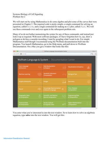
Systems Biology of Cell Signaling Problem Set 2 We will start out by using Mathematica to do some algebra and plot some of the curves that were presented in Chapter 2. The required code is pretty simple--a single command for solving an equation, called Solve, and a single command for making an x-y plot, called Plot. We will use these commands over and over again in the subsequent problem sets. Many of us do not bother memorizing the syntax for any of these commands, and instead just look it up as required. With most software packages, if I have forgotten how to, say, draw a polygon or de-hiss a cassette recording, I start by googling what I want to do. For simple Mathematica stuff though I recommend using the Wolfram documentation built into the program. You launch Mathematica, go to the Help menu, and pull down to Wolfram Documentation. On a Mac you get a window that looks like this:
You enter what you’re interested in into the text window. So to learn how to solve an algebraic equation, type solve into the text window. You will get this:
Information Classification: General
2
The first “basic example” shows us everything we need to know for now. You type Solve, with a capital S--all of the Mathematica commands start with capital letters. Then type an open square bracket, then an equation with a double equal sign, then the variable you want Mathematica to solve for, and then a close square bracket. In the example equation, they use a space to represent the multiplication sign between a and x. I recommend against this; it’s much easier to see that you have entered the multiplication expression correctly if you type it as a*x, using the asterisk as a multiplication sign. And finally, you type an Enter—Shift-Return on a Mac. Lo and behold Mathematica spits out the solution or solutions of your equation. We will now use the Solve command to work through some of the derivations from Chapter 2. 1. Suppose we have a ligand x binding to a receptor y to form a complex cxy. In Chapter 2 we wrote down the rate equation for this process, and then set it equal to zero to yield an algebraic equation for the conditions required for equilibrium. This yielded Eq 2.5: (2.5)
Information Classification: General
3 Use the Solve command to get an expression for cxy in terms of ytot, x, and the kinetic parameters.
2. Plot the equation you just derived using the Plot command for some choice of parameters--for simplicity let’s say k1 = k-1 = ytot = 1. You can assign these values this way:
Note that we have put three separate commands, on three separate lines, in one Input cell for convenience. And note that here you need to use a single equal sign rather than a double equal sign (it’s an issue of whether you are defining a mathematical relationship between two sides of an equation or assigning a numerical value to a variable/parameter). You should be able to get all the syntactical help you need for the Plot command from the Wolfram Documentation Center. Choose a reasonable range for the x-axis--say 0 to 10, the way it is in Fig. 2-4a.
3. The Plot command includes many options. One very useful option is PlotRange, which you can use to specify the range of y-axis values you want to see. If you don’t specify it, Mathematica will guess at what is the most interesting part of the plot and show that to you, and it doesn’t always guess right.
Information Classification: General
4 Use PlotRange to make the y-axis range be 0 to 1. Note that to make the right arrow for this option, you type a hyphen followed immediately by a greater than sign (->).
4.
Use the PlotStyle option to make your curve green.
5. Now let’s try upping the value of k1 to 10. Plot the resulting curve, and make it red. Use the same range of x and y values.
Information Classification: General
5
6.
Combine the two curves together on a single plot using the Show command.
7.
Plot the same two curves on a semi-log plot using the LogLinearPlot command.
Information Classification: General