Solution Manual For Mastering ArcGIS Pro 2e Release 2025 Maribeth Price Chapters 2-12
Chapter 1 Answers to Exercises 1
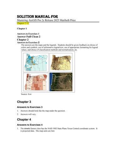
Answer Full Clean 2 Chapter 2 Answers to Exercises 2 The answers are the maps and the legends. Students should be given feedback on choice of colors and symbols, use of informative legend text, use of appropriate formatting for legend values, and choice of classification methods and normalization, etc.
Source: Esri
Chapter 3 Answers to Exercises 3 1. Answers should look like the map under the question. 2. Answers will vary.
Chapter 4 Answers to Exercises 4 1. The streets feature class has the NAD 1983 State Plane Texas Central coordinate system. It is projected data. The map units are feet.
Method: Right-click the data set in the Contents pane, open its properties, and examine the Coordinate Systems settings. 2. The projection is Lambert Conformal Conic. It has a central meridian of -120.5 and standard parallels of 43 and 45.5. No, it uses 41.75 as its latitude of origin. Method: Right-click one of the data set in the Contents pane, open its properties, and examine the Coordinate Systems settings. 3. The DMS coordinates are 121° 45’ 38‖ W, 46° 51’ 10‖ N. The UTM coordinates are about 594,490E and 5,189,560N. The State Plane coordinates are about 1,325,060E and 556,660N. Method: Use the Locate tool to search for and find Mt. Rainier, then zoom in close to find the point marking the summit on the Topographic base map. Open the map properties and set the coordinate system to GCS NAD 1983, place the cursor on the summit, and read the x-y display values. Repeat for the other two coordinate systems and units. 4. They have the same central meridian, false easting, and false northing, but the standard parallels are different: 33 and 44 for the contiguous US and 20 and 60 for North America. The parallels are wider apart because North America covers a wider range of latitudes and the parallels should be placed at the upper and lower sixths. The latitude of origin is also slightly different, 39 versus 40, so that it is centered between the parallels. Method: Open the map properties and select each coordinate system in turn. Click the Details link to view the parameters for each one and compare what you find. 5. The central meridian is 25 and the standard parallels are 20 and -23. The Latitude of Origin is the equator. Yes, it will have negative y values because the latitude of origin is the equator and a good portion of Africa lies below it. Method: Open the map properties and select the coordinate system. Click the Details link to view the parameters. 6. It is a secant conic projection because it has two standard parallels. Method: Open the map properties and select the coordinate system. Click the Details link to view the parameters. 7. It uses the WGS 84 datum because the NAD 1983 datum used in the US projections is optimized for North America and does not work well elsewhere. Method: Open the map properties and select the coordinate system. Click the Details link to view the parameters. 8. The projections are as follows a. Amarillo lies near the boundary between UTM Zones 13 and 14, but near the center of the Texas State Plane North zone. Distortion would be less for the State Plane zone. b. Pensacola, Florida is at the far west end of the Florida North State Plane Zone but almost at the center of the UTM Zone 16 Zone, so UTM would be better. c. The state of Tennessee nearly fits within the UTM Zone 16 but extends further east. Also, it is an elongated east-west area, so the conic State Plane zone would be preferred. Method: For the US areas, add the utmzone and spcszones layers and symbolize and label them for easy viewing. Search for the locations and determine whether they are closer to the center of the State Plane or the UTM zone. 9. Mississippi runs north-south. Start with the Mississippi East or West State Plane zone and modify the central meridian to the approximate center of the state, about -89.7. The answer should appear similar to the picture.
Source: Esri 10. The dog_offleash_areas point file has an undefined coordinate system, although it appears to be in NAD 1983 State Plane Texas Central like the other Austin data. The dog_offleash_bnd polygon file is in an unlabeled GCS. The other answer is the map. Method: Load the arteries into a new map document. Add the dog point file, which appears but with a warning. Examine the coordinate system to determine that it is unlabeled, and use Define Projection to set it to match the other Austin data in State Plane. Add the dog polygon file, which does not appear. Examine the coordinate system to determine that it is unlabelled and contains degrees. Use Project Define to label it as GCS_NAD_1983, and it then appears with the rest of the data. It can be projected to State Plane if desired, but it is not necessary to make the map.
Source: City of Austin, TX
Chapter 5 Answers to Exercises 5 Answers will vary.
Chapter 6 Answers to Exercises 6 Answers will vary.
Chapter 7 Answers to Exercises 7 1. Method: Add the table to Pro and use the Export function to save it in the geodatabase. 2. There are 3176 stores. The first one opened in Rogers, Arkansas in 1962. The latest one opened on January 31, 2006 in ten different locations. Method: Look at the number of records in the table to determine the number of stores. Sort by the OPENDATE field to find the earliest and latest openings. 3. The latest date is not the actual youngest store(s). The metadata indicates that store openings until 2006 are included. The count will not include new stores opened since then. Method: Use the Catalog view to examine the metadata for the .csv file. 4. Texas has the most stores, 315. Method: Use the Frequency tool to count the stores, with STRSTATE as the case field. 5. Arkansas has the most stores per capita, 2.7 per 100,000 people. California has the least, with 0.4. Method: Create a per capita field in the stores table. Join states to the stores table with stores as the target. Calculate the per capita field using stores.frequency / states.POP2014 * 100000.
6. See maps. The numbers map appears mostly but not completely related to population, an example of MAUP issues. The per capita map suggest that the stores are much stronger and more prevalent in the Midwest than in the Pacific states and most of the northeast. Method: Remove the previous join with stores as the target table and add a new join with states as the target table. Create a map based on the frequency field. Then remove the previous join with stores as the target table and add a new join with states as the target table. Create a map based on the frequency field. Map of the number of Walmarts per state
Source: Esri Map of Walmarts per capita
Source: Esri 7. See plot. There is a fairly strong correlation with an R-squared of 0.62. Texas lies above the line and has far more stores than expected. California and New York lie below the line and have far fewer stores than expected.