1
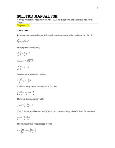
Solution Manual For Applied Numerical Methods with MATLAB for Engineers and Scientists 5e Steven Chapra Chapters 1-24 CHAPTER 1 1.1 You are given the following differential equation with the initial condition, v(t = 0) = 0, c dv g d v2 dt m
Multiply both sides by m/cd m dv m g v2 cd dt cd
Define a mg / cd m dv a2 v2 cd dt
Integrate by separation of variables, cd
a v m dt dv
2
2
A table of integrals can be consulted to find that
a x a tanh a dx
2
1
1 x
2
Therefore, the integration yields 1 v c tanh 1 d t C a a m
If v = 0 at t = 0, then because tanh–1(0) = 0, the constant of integration C = 0 and the solution is 1 v c tanh 1 d t a a m
This result can then be rearranged to yield v
gcd gm tanh t m cd
2
1.2 (a) For the case where the initial velocity is positive (downward), Eq. (1.21) is
c dv g d v2 dt m Multiply both sides by m/cd m dv m g v2 cd dt cd
Define a =
mg / cd
m dv a2 v2 cd dt
Integrate by separation of variables,
cd
a v m dt dv
2
2
A table of integrals can be consulted to find that
a x a tanh a dx
2
1
1 x
2
Therefore, the integration yields
1 v c tanh 1 d t C a a m If v = v0 at t = 0, then
C
v 1 tanh 1 0 a a
Substitute back into the solution
v 1 v c 1 tanh 1 d t tanh 1 0 a a m a a Multiply both sides by a, taking the hyperbolic tangent of each side and substituting a gives,
v
gcd cd mg tanh t tanh 1 v0 cd mg m
(1)
3
(b) For the case where the initial velocity is negative (upward), Eq. (1.21) is
c dv g d v2 dt m Multiplying both sides of Eq. (1.8) by m/cd and defining a mg / cd yields
m dv a2 v2 cd dt Integrate by separation of variables,
cd
a v m dt dv
2
2
A table of integrals can be consulted to find that
a x a tan a dx
2
1
1 x
2
Therefore, the integration yields
1 v c tan 1 d t C a a m The initial condition, v(0) = v0 gives
C
v 1 tan 1 0 a a
Substituting this result back into the solution yields
v 1 v c 1 tan 1 d t tan 1 0 a a m a a Multiplying both sides by a and taking the tangent gives v c v a tan a d t tan 1 0 a m
or substituting the values for a and simplifying gives
v
gcd cd mg tan t tan 1 v0 cd mg m
(2)
(c) We use Eq. (2) until the velocity reaches zero. Inspection of Eq. (2) indicates that this occurs when the argument of the tangent is zero. That is, when
4
gcd cd t zero tan 1 v0 0 m mg The time of zero velocity can then be computed as
t zero
cd m tan 1 v0 gcd mg
Thereafter, the velocities can then be computed with Eq. (1.9), gcd mg v tanh (t t zero ) cd m
(3)
Here are the results for the parameters from Example 1.2, with an initial velocity of –40 m/s.
t zero
68.1 0.25 tan 1 (40) 3.470239 s 9.81(0.25) 68.1(9.81)
Therefore, for t = 2, we can use Eq. (2) to compute
v
9.81(0.25) 68.1(9.81) 0.25 m tan (2) tan 1 ( 40) 14.8093 0.25 68.1 68.1(9.81) s
For t = 4, the jumper is now heading downward and Eq. (3) applies
v
9.81(0.25) 68.1(9.81) m tanh (4 3.470239) 5.17952 0.25 68.1 s
The same equation is then used to compute the remaining values. The results for the entire calculation are summarized in the following table and plot: t (s)
v (m/s)
0 2 3.470239 4 6 8 10 12
-40 -14.8093 0 5.17952 23.07118 35.98203 43.69242 47.78758
5
60 40
20 0
-20 0
4
8
12
-40
1.3 (a) Use the conservation of cash to compute the balance on 6∕1, 7∕1, 8∕1, and 9∕1 if the interest rate is 1% per month (i = 0.01∕month). Show each step in the computation. (b) Write a differential equation for the cash balance in the form
dBi f [ D(t ),W (t ), i] dt where t = time (months), D(t) = deposits as a function of time ($/month), W(t) = withdrawals as a function of time ($/month). For this case, assume that interest is compounded continuously; that is, interest = iB. (c) Use Euler‟s method with a time step of 0.5 month to simulate the balance. Assume that the deposits and withdrawals are applied uniformly over the month. (d) Develop a plot of balance versus time for (a) and (c). ========================================== (a) This is a transient computation. For the period ending June 1: Balance = Previous Balance + Deposits – Withdrawals + Interest Balance = 1512.33 + 220.13 – 327.26 + 0.01(1512.33) = 1420.32 The balances for the remainder of the periods can be computed in a similar fashion as tabulated below: Date 1-May
Deposit
Withdrawal
Interest
$220.13
$327.26
$15.12
$216.80
$378.61
$14.20
$450.25
$106.80
$12.73
$127.31
$350.61
$16.29
1-Jun
$1,420.32
1-Jul
$1,272.72
1-Aug
$1,628.89
1-Sep
(b)
Balance $1,512.33
dB D(t ) W (t ) iB dt
(c) for t = 0 to 0.5: dB 220.13 327.26 0.01(1512.33) 92.01 dt
$1,421.88