Issuu

XII

https://doi.org/10.22214/ijraset.2021.39593

December 2021

CNN-Enhanced Multi-Indices Patch-Based Classification: A Case Study of Guwahati City Arindom Ain1, Minakshi Gogoi2, Dibyajyoti Chutia3 1, 2

Dept. of Computer Science & Engg., GIMT, Guwahati Guwahati-781017, Assam, India

Scientist/Engineer SF North Eastern Space Applications Center, Department of Space Umium, Shillong, India

Abstract: Land use and land cover (LULC) provides a way to classify objects on the surface of Earth. This paper aims to identify the varying land cover classes by stacking of 6 spectral bands and 10 different generated indices from those bands together. We have considered the multispectral images of Landsat 7 for our research. It is seen that instead of using only basic spectral bands (blue, green, red, nir, swir1 and swir2) for classification, stacking relevant indices of multiple target classes like ndvi, evi, nbr, BU, etc. with basic bands generates more precise results. In this study, we have used automated clustering techniques for generating 5 different class labels for training the model. These labels are further used to develop a predictive model to classify LULC classes. The proposed classifier is compared with the SVM and KNN classifiers. The results show that this proposed strategy gives preferable outcomes over other techniques. After training the model over 50 epochs, an accuracy of 93.29% is achieved. Keywords: Land use, land cover, CNN, ISODATA, indices I. INTRODUCTION Conserving Natural resources are an important element for environmental aspects. Different activities have been carried out by humans using various naturally existing resources in the environment. So monitoring and proper utilization of resources are necessary to maintain sustainable growth in the environment [1]. One of the effective methods suggested by the literature is by using areal images [2]. The changes that occur in the earth’s surface are caused due to evolution and are recognized as LULC changes. Areal images collected from the satellite could be used for LULC map generation [1], [2]. The LULC maps have a great impact in monitoring, management, and planning programmes at both local and national levels [3], [4], [5]. With the evolution of remote sensing technology, the generation of LULC maps over time became very efficient. LULC maps are efficient in terms of monitoring and planning activities, ecosystem management, climate change, and government policies [3]. In this paper, we intend to do a case study of the GM region, a prominent city of the North Eastern Region (NER) about the urban growth, agriculture, watershed, and bare land using multispectral satellite images. Many development activities are going on at Guwahati city [6]. An extension is planned under a Master Plan-2025 concerning smart city development. The city is listed in the "smart cities" category among t h e top 20 cities [7, 8]. With development, the prospect of urbanization and urban growth increases with time. So, we feel it is important to do proper assessment and planning for better development of the region. With this objective, it is proposed to develop an efficient deep learning model for the detection and classification of LULC classes and generate a LULC classification map for the GM region. LULC is primarily classified into four classes based on different signature viz, land, water, vegetation, and built-ups. North-East India is rapidly facing a transition from one class to another over time due to the influence of many factors on the base class. Factors can be classified into two major types viz. direct influencing factor (DIF) and indirect influencing factor (IIF). DIF is categorized as those factors which directly influence the transitions of classes and IIF are those which indirectly affect the transition. We have selected some DIF and IIF to understand and listed them in Table I. Due to these factors, NER is facing many challenges like improper field survey, smart and proper planning of roads, water conservation, dams, and other construction, access to unreachable areas, land cover changes monitoring, land use detection, flood problems, etc. These challenges result in some direct or indirect issues like increasing pollution, destruction of natural habitat, illegal settlements, eco-system disruption, and state economy slowdown by proper monitoring and analysis of the LULC map over time. Many works of literature [9, 10, 11, 12] have found remote sensing and GIS techniques as an adequate method of analyzing land use and land cover detection and classification. Guwahati Metropolitan (GM) is one of the renowned cities situated in the state of Assam of NER. It has undergone immense expansion due to rapid urbanization and other human needs [6]. For the last decades, the city has been known to have a relatively sparse population.

©IJRASET: All Rights are Reserved | SJ Impact Factor 7.538 | ISRA Journal Impact Factor 7.894 |

1824

International Journal for Research in Applied Science & Engineering Technology (IJRASET) ISSN: 2321-9653; IC Value: 45.98; SJ Impact Factor: 7.538 Volume 9 Issue XII Dec 2021- Available at www.ijraset.com But now it falls under the category of the fastest growing city in the north-eastern region. So, it becomes important to detect and monitor the nature and frequency of changes to predict and analyze the direction of future expansion. With these aims, we have come up with the following objectives listed below. 1) Collecting and selecting Landsat Satellite images of GM region 2) Preprocessing of collected satellite images. 3) Preparing Labels for supervised learning and validating class labels from field surveys and high-resolution maps in an unsupervised way. 4) Land use Land cover detection, prediction, and classification. 5) Accuracy assessment. 6) Analysis 7) Comparison with other techniques The rest of the paper is organized into sections. Section II will discuss the related literature. Section III will give an introduction of the study area and its importance and Section IV discuss the motivation and methodology. Section V focus on the results and analysis. Section VI will discuss the comparison of our model with other techniques and lastly, section VII has the conclusion. TABLE I LAND COVER INFLUENCING FACTORS Direct Influencing Factors Indirect Influencing Factors Increasing flood Soil erosion in Brahmaputra River Habitat destruction Landslide activity

Weak society economy the Improper Planning Sport and communication disruption. Monitoring Problems

II. LITERATURE STUDY The classification of satellite images involves the classification of the binary class of categorical classes. The binary class classification is generally done for Built-up area or Water bodies segmentation from satellite images. With the recent enhancement of various machine learning techniques, the LULC mapping for multiple classes has been attracting considerable attention. Yansheng et al [13] proposed Multi-Label Remote Sensing Image Scene Classification by Combining a Convolutional Neural Network and a Graph Neural Network. [14] included NDVI, MNDWI, NDBI, and Sentinel 2A bands to classify vegetation, water, and built-up areas. He used a multilayered feed-forward deep neural network to classify different Land Cover classes. Literature also suggested the use of pre-trained models like VGG16, Inception-ResNet-V2, Inception-V3, and DenseNet201 to extract features from satellite data [15]. The multispectral data can be classified using a supervised or unsupervised learning approach. The supervised classification can be done either traditional pixel-wise or patch-based. In pixelwise classification, each pixel is individually mapped with the corresponding spectral data. Many machines learning models like random forest, support vector machines, and self-organizing maps use this approach for learning. But this approach does not consider spatial information completely in learning as cand cover pixels may correlate with neighboring pixels [16]. Another approach is patch-based that uses spatial patterns in classification. Here instead of using individual pixels for learning, it also includes the neighboring pixels to extract information to learn. 2D-CNN can be used to extract features from neighboring pixels. It uses multiple layers to learn. This study includes multispectral data, i.e., the dataset will consist of multiple bands to form a 3D structure. This structure is fed to CNN to extract features. Many pieces of the literature suggested the use of spectral indices to classify land cover classes [17, 18]. [17] used water indies TCW, NDVI, MNDWI, AwEisnh, Aweish, and WRI for mapping urban areas and watersheds. They have used a supervised classification-based Minimum Distance algorithm in ArcGIS to map the water bodies. Indices like Automated Built-up Extraction Index (ABEI) [19], Normalized Difference built-ups Index (NDBI) [20], Index-Based Built-up Index (IBI) [21], and Modified Built-Up Index (MBUI) were developed to classify built-up class and other class in satellite images [18].

©IJRASET: All Rights are Reserved | SJ Impact Factor 7.538 | ISRA Journal Impact Factor 7.894 |

1825

International Journal for Research in Applied Science & Engineering Technology (IJRASET) ISSN: 2321-9653; IC Value: 45.98; SJ Impact Factor: 7.538 Volume 9 Issue XII Dec 2021- Available at www.ijraset.com In this research, we include 10 sets of indices including 6 Landsat bands. Though some work used indices for specific class classification [17,18,20]. We have combined specific indices relevant to each class for multiclass classification. It is seen that fusion of these multiple indices shown in table III, with basic spectral bands shows impressive result. The proposed architecture can handle input data with no-data pixels. It is seen that the proposed technique outperforms many states of art algorithms, such as SVM and KNN. III. STUDY AREA Guwahati is the main hub and metropolis in Assam and Northeast India. It can be called the heart of the North-Eastern region. It comes under the jurisdiction of the Guwahati Metropolitan Development Authority (GMDA). The total area of it is around 216 Sq. Km. The approximated population density according to the 2011 census is about 1 million and was estimated to grow million by 2025 [7]. The city is bounded on the northern side by the great river Brahmaputra, and on the southern side by hill rocks that are extensions of the Khasi highlands. The Rani Reserve Forest, Deepor Beel wetland, and alluvial tracts of the Brahmaputra plain are located in the west and southwest. Many endangered birds and rare animals as Asian elephants, pythons, and one-horned rhino can be found in the Guwahati region. The city has been divided by Guwahati Municipal Corporation into five divisions within which twenty zones and sixty wards are demarcated for better service. The Guwahati city map with true color is shown in Figure 2. The map is created by overlapping administrative boundary vector data collected from OpenStreetMap on Landsat 7 satellite image. IV. MOTIVATION AND METHODOLOGY For decades it is seen that changes in particular land cover classes are always impacted or come under the influence of either naturally occurring factors or man-made factors over time. Naturally occurring factors like climate change, sudden earthquakes, landslides, increasing flood, water source, soil erosion is a major river, etc., and man-made factors like industries setup, infrastructure setup, communication channel, population, illegal settlements, etc., [22]. Also, the same LC class is influenced by its surrounding classes over time [10]. Some indirect factors are also responsible for the changes like weak society economy, improper planning, sports and communication disruption, monitoring problem, etc. Due to these naturally occurring, man-made, and indirect factors, the area is affected by many challenges, especially in NE states. As NE is surrounded by rivers and mountains, it becomes very challenging to proper field study and faces monitoring problems. Due to these challenges, NE is facing some issues like increasing population, destruction of natural habitat, illegal settlements, ecosystem disruption, etc. Guwahati city is one of the prominent hubs of State Assam in the NE region because of state economic, industrial prospect, main communication gateway for other NE states, heritage like Maa Kamakhya temple and Ramdesir site Deepor Beel. So, for the prospect of urbanization and to continue to maintain the existence of ecologically sensitive areas, it is important to do proper assessment and planning for better development of the city. Many kinds of literature have found remote sensing and GIS techniques as an adequate method of LULC detection, classification, and analysis [1, 3, 6, 9]. So, we have considered developing a model based on deep learning which could be able to classify and predict different land cover classes. The architecture of the proposed methodology is shown in Figure 1. The proposed methodology is composed of mainly three sections as described below. 1 ) Preprocessing of satellite images

Model Training 3 ) Model Testing 2)

A. Preprocessing of Satellite Images Preprocessing of satellite data plays an important role in the analysis of final output. In this study, the preprocessing of Landsat imagery involves the following steps. 1) Creation of Guwahati City Boundary Vector File: As for downloading and extracting the raster data of the study area, we need to specify the extent of the target location. So, we have extracted the polygon of the administrative boundary of Guwahati city from the OSM layer [23]. This extracted polygon is saved as a vector file Vs for further use. The algorithm for the creation of the boundary vector file is given in Algorithm 1

©IJRASET: All Rights are Reserved | SJ Impact Factor 7.538 | ISRA Journal Impact Factor 7.894 |

1826

Data Source: Satellite data can be collected from various web sources namely, USGS [24, 25], etc. We have collected multispectral Landsat imagery of the Guwahati city location for the year 2011. The imagery is freely available at this website address http://www.earthexplorer.usgs.gov. For the year 2011, we have used Landsat 7 satellite images. It comprises multispectral sensors that collect 6 spectral bands viz, Blue, Green, Red, NIR, SWIR1, SWIR2. All the bands have t h e same spatial resolution of 30 meters but with different spectral properties. The maps generated are projected in the WGS84 UTM 46N projection. To download the Landsat tile containing the study area, we have used the vector file Vs in USGS. It is seen from the footprint of tiles that in the NE region we can find images with very less cloud cover from January to April. So, the tiles are collected between January to April do not contain any cloud cover on the study boundary. The complete Guwahati administrative boundary fits into a single tile. The metadata information of the tiles downloaded is given in Table II. Image Correction: It generally involves the atmospheric correction of overall images. Moreover, radiometric calibration and corrections [4] are important for classification. Landsat 8 has a higher radiometric and spectral resolution. So, to keep it simple we have selected Landsat 7 images for our research [26]. The raster data of the target area fetched with 0% cloud cover is referred to in Table II, so we could infer that no effect of cloud on the raster data of the study area. Many researchers have suggested the use of Semi-Automatic Classification to perform DOS1 atmospheric correction and conversion of DN number to the reflectance of Landsat images [27]. To keep it simple we have set the "No Data" pixels to value. And also, we have considered the "No Data" value as a classification label and feed to the deep learning algorithm. The algorithm for image correction is given in Algorithm 2. Clipping of Study Area: The corrected raster contains pixels outside the study area boundary. For processing, the unwanted pixel is an extra overhead. So, we clipped the exact study area raster extent by overlapping the vector shapefile Vs of Guwahati city that is generated earlier on the corrected raster. The clipped raster is then ready for further processing. The algorithm for clipping the GM raster based on GM boundaries is given in Algorithm 3 Generating Features for Model Training: In this study, we have considered both spectral and spatial characteristics of satellite images as features. The spectral indices like NDVI, NDWI, etc. were explored from the aspect of water body cover(W), forest cover(F), vegetation cover(V), and built-up areas (BU) using Landsat data. So, it is assumed that the indices will help in enhancing the accuracy of the influence of LC classes during generating model. All the indices for each raster data are computed and stacked together along with raster data. All the bands that are used in the calculation of index values have the same spatial resolution. Every indices have limitations. Like NDVI is highly sensitive to the brightness of soil and atmospheric effect, so we have considered some other indices, viz, MSAVI, EVI, ARVI, and NBR along with NDVI for more accurate classification of vegetation. Similarly, for identification of water features, water index like the NDWI (normalized difference water index), MNDWI (modified NDWI) [28, 29, 30, 31, 32] are considered. Built-up index enhances the spectral characteristics of built-up areas [33]. All the bands viz. blue, green, red, NIR, SWIR1 and SWIR2 of 2011 is than stacked with the generated indices map ARVI, AWEIsh, BI, EVI, MNDW2, MSAVI, NBR2, NBR, NDVI, NDWI in one file Rraster. The bands and indices used in this literature are shown in Table III. Label Creation for Supervised Learning: The labels for training are generated by using an unsupervised learning approach. Kmeans clustering and Iterative Self Organizing Data Analysis Technique (ISODATA) are two algorithms that can be used for the cluster creation in unsupervised classification [39]. We have used the ISODATA algorithm to find 5 different clusters. The signature is seeded from band values of Landsat 7 satellite data. The minimum distance between the signature i s u s e d w i t h a distance threshold value of 0.01 and a maximum standard deviation of 0.02 for finding the 5 different clusters. For verifying the identified and mapped landscapes class with actual raster data, we have used high resolution google earth images. The pixels of cluster corresponding to vegetation area in google map is labeled as V for vegetation, the cluster pixels corresponding to water bodies in google map is marked W for water bodies. Similarly, built-ups as B and land as S. The no data is treated as label as D. Finally, we got a labelled map Rlabel of timeline 2011 with five different class pixels (V, W, B, S, and D) based on signature similarity and dissimilarity. This labelled map generated is also verified by masking it with the LULC thematic map downloaded from the website https://bhuvan-app1.nrsc.gov.in/thematic/thematic/index.php [25].

©IJRASET: All Rights are Reserved | SJ Impact Factor 7.538 | ISRA Journal Impact Factor 7.894 |

1827

1 2 3 4 5 6

Bands and Indices Blue Green Red NIR SWIR1 SWIR2

ARVI

Serial No

MNDWI

− 1.5 ∗ ( 2)

+ 1 − (2 ∗

NBR

NDVI

NBR2

)+1

1 1

Enhancement of open water features.

−

on land surface [22], [8]. NDWI (Normalized Difference Water Index) enhances the water features of the landscapes[38]

− + − + ( (

MSAVI (Modified Soil-Adjusted Vegetation Index) to reduce the soil noise influence like, soil color, soil variability across region, soil moisture on canopy spectra [37]. NBR (Normalized Burn Ratio) index is used to highlight the areas that are burned either due to human needs or due to wild- fires destroying forest biomass and is used in agriculture and forestry in the detection of active fires, analysis of burn severity, and monitoring of vegetation survival after the burn. NDVI used to estimate the green area density

− +

( (

EVI (Enhanced Vegetation Indices) is used in areas where leaf area index content is high. The blue band is used to rectify soil background signals and influence of atmosphere [36].

)

− +

NDWI

+ 1) − 8 ∗ ( 2

MSAVI

)+ )+

− + 2∗

Landsat 7 Band Landsat 7 Band Landsat 7 Band Landsat 7 Band Landsat 7 Band Landsat 7 Band ARVI (Atmospherically Resistant Vegeta- tion Index) is effective for regions that are polluted This indices is well known for classification of areas with shadow and dark surfaces. AWEIsh is intended to eliminate shadow pixels [35].

2.5 ∗ ( − +6∗ − 7.5 ∗

( EVI

+ 2.5 ∗ ) − 0.25 ∗

AWEISH

Description

− (2 ∗ + (2 ∗ (

Formulae

) ( − ) ( 1− 1+

− + 2) 2)

) )

The Built-up (BU) index is the binary image having higher positive value. It indicates built-up area and barren land, allowing BU to map the built-up area automatically [33]. Normalized Burn Ratio (NBR) 2 is used to highlight water sensitivity in vegetation.

©IJRASET: All Rights are Reserved | SJ Impact Factor 7.538 | ISRA Journal Impact Factor 7.894 |

1828

International Journal for Research in Applied Science & Engineering Technology (IJRASET) ISSN: 2321-9653; IC Value: 45.98; SJ Impact Factor: 7.538 Volume 9 Issue XII Dec 2021- Available at www.ijraset.com 7) Generation of 3D Raster Patches and Corresponding 2D Label Patches: The stacked raster data Rraster (Rrow x Rcolumnx Rbands) is split to 3D patches p0 ,p1,p2,p3. . . .pn−1. We considered each patch has a size (7x7xRbands). The patches are created with a stride similar to patch row size as shown in equation 1. Therefore, Rraster = p0, p1, p2, p3 . . . .pn−1

(1)

Similarly, the label 2D data Rlabel is also divided into l number of patches shown in equation 2. The patches created for the label have the same dimension as that of Rraster i.e (7x7). They are also created with a stride similar to the patch row size of Rraster . given by equation 2. = , , ,…. ( ) Further to include the influence of surrounding raster on raster center pixel in classification, the central pixel of each patch of labels is extracted. To find the central pixel index position equation 3 is used patch + 1 patch +1 (3) = , 2 2 7+1 7+1 = , 2 2 = (4,4)

©IJRASET: All Rights are Reserved | SJ Impact Factor 7.538 | ISRA Journal Impact Factor 7.894 |

1829

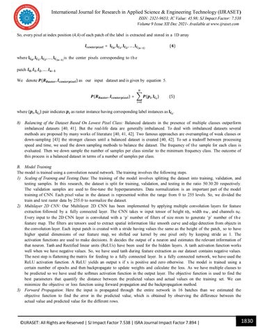
International Journal for Research in Applied Science & Engineering Technology (IJRASET) ISSN: 2321-9653; IC Value: 45.98; SJ Impact Factor: 7.538 Volume 9 Issue XII Dec 2021- Available at www.ijraset.com So, every pixel at index position (4,4) of each patch of the label is extracted and stored in a 1D array = where patch

,…,

(

)

,…,

(

( )

)

is the center pixels corresponding to t h e

, , ,….

We denote (

) as our input dataset and is given by equation 5.

(

where ( ,

) pair indicates

( ,

)

as raster instance having corresponding label instances as

(5)

8) Balancing of the Dataset Based On Lowest Pixel Class: Balanced datasets in the presence of multiple classes outperform imbalanced datasets [40, 41]. But the real-life data are generally imbalanced. To deal with imbalanced datasets several methods are proposed by many works of literature [40, 41, 42]. Two famous approaches are oversampling of weak classes or down-sampling [43] the stronger classes until a balanced dataset is created [40, 42]. To set a tradeoff between processing speed and time, we used the down sampling methods to balance the dataset. The frequency of t h e sample for each class is evaluated. Then we down sample the number of samples per class similar to the minimum frequency class. The outcome of this process is a balanced dataset in terms of a number of samples per class. B. Model Training The model is trained using a convolution neural network. The training involves the following steps. 1) Scaling of Training and Testing Data: The training of the model involves splitting the dataset into training, validation, and testing samples. In this research, the dataset is split for training, validation, and testing in the ratio 50:30:20 respectively. The validation samples are used to fine-tune the hyperparameters. Data normalization is an important part of the model training of CNN. Each pixel value in the dataset is represented within the range from 0 to 255 levels. So, we divided the train and test raster data by 255.0 to normalize the dataset. 2) Multilayer 2D CNN: Our Multilayer 2D CNN has been implemented by applying multiple convolution layers for feature extraction followed by a fully connected layer. The CNN takes w input tensor of height nh, width nw , and channels nc. Every input to the 2D CNN layer is convoluted with a ‘p’ number of filters of size mxm to generate ‘p’ number of t h e feature map. The filters are tensors used to extract spatial information like smooth curve and edge detection from objects in the convolution layer. Each input patch is created with a stride having values the same as the height of the patch, so to have higher spatial dimensions of our feature map, we shifted our kernel by one pixel only by keeping stride as 1. The activation functions are used to make decisions. It decides the output of a neuron and estimates the relevant information of that neuron. Tanh and Rectified linear units (ReLUs) have been used for the hidden layers. A tanh activation function works well when we have negative values. So, we have used tanh during feature extraction as our dataset contains negative values. The next step is flattening the matrix for feeding to a fully connected layer. In a fully connected network, we have used the ReLU activation function. A ReLU yields an output x if x is positive and zero otherwise. The model is trained using a certain number of epochs and then backpropagate to update weights and calculate the loss. As we have multiple classes to be predicted so we have used the softmax activation function in the output layer. The objective function is used to find the best parameters that quantify the distance between the predicted values and actual values on the training set. We can minimize the objective or loss function using forward propagation and the backpropagation method. 3) Forward Propagation: Here the input is propagated through the entire network in 16 batches than we estimated the objective function to find the error in the predicted value, which is obtained by observing the difference between the actual value and predicted value for the different rows.

©IJRASET: All Rights are Reserved | SJ Impact Factor 7.538 | ISRA Journal Impact Factor 7.894 |

1830

Backpropagation: It consists of finding the gradients of the cost function for different parameters and then applying a gradient descent algorithm to update the weights. The same process is iterated several times called epoch number. The softmax function has been used in the output layer of CNN because more than two classes are to be classified. The parameters used in each layer of this architecture are given in Table IV. The architecture involves 3 convolution layers followed by dense layer and output layers. Input patch of size 7x7x16 has been given to the first Convolutional Layer. The Convolution layers have 16,32,48 filters followed by a fully connected layer, consisting of 1000 nodes. The model is trained on total {779989} parameters with batch sizes 16 and 50 epochs. The learning rate is set to be 0.0001. We have used ‘Adam’ as a model optimizer. The description of each layer is described below. The last layer contains five nodes with a softmax activation function. It produced 5005 parameters. The loss function used in this architecture is ’categorical_crossentropy’.

C. Model Testing The model is tested on a different set of unseen data. The result is evaluated using various metrics and is discussed in the results section

TABLE II LANDSAT TARGET AREA TILE INFORMATION Year 2011 Data Set Attribute Attribute Value Acquisition Date 4/7/2011 Satellite 5 Collection Category T1 Sensor Mode BUMPER WRS Path 137 WRS Row 42 Land Cloud Cover 6 Study Area Cloud Cover 0 Sensor Identifier TM

Class Water Vegetation Built-up Land Others

TABLE V PIXEL AREA Pixel sum 7945 43219 20035 11279 163267

Area (SQ meter) 7150500 38897100 18031500 10151100 146,940,300

©IJRASET: All Rights are Reserved | SJ Impact Factor 7.538 | ISRA Journal Impact Factor 7.894 |

1831

International Journal for Research in Applied Science & Engineering Technology (IJRASET) ISSN: 2321-9653; IC Value: 45.98; SJ Impact Factor: 7.538 Volume 9 Issue XII Dec 2021- Available at www.ijraset.com Algorithm 1 Creation of Guwahati city boundary vector file Input: O: OpenStreetMap of Kamrup Metropolitan district with attribute administrative boundary O Output: Vector file of Guwahati city boundary extent Process: 1) Initialized OSM layer O= , , , … where O ∈ set of points of the polygon of Guwahati City boundary in OSM ranging from 1 to n 2) Initialized a new vector file v 3) for each point i in O till n, do 4) if is the starting point then: 5) v = v0 6) else if vi = v0 then: 7) stop loop 8) else: 9) v.append(vi) 10) v = v + vi 11) Save vector v as Vs Algorithm 2 Algorithm for Image correction (Consider red, green, blue, NIR, SWIR1, SWIR2, and Band 1, 2, 3, 4, 5, 6 respectively) Input: I: uncorrected satellite image multitemporal with ‘r’ rows from 1 → p and ‘c’ columns from 1 → q and z bands with bands 1,2,3,4,5,6 where p = max(r) and q = max(c) Output: Corrected satellite image (multitemporal) Process: 1) 2) 3) 4) 5) 6) 7) 8) 9) 10) 11) 12) 13) 14) 15)

Initialized r → 1 and q → 1and z → 1 for each band in z ∈ I do for each row r ∈ I do for each pixel p in column c ∈ I do Load pixel p at r ∗ c if valuesat(p) == ’No Data’ than: Set ’No Data’ to value 0 at p Check for atmospheric error on p Geometric Resampling and Adjustment on p Convert to reflectance End for of c End for of r End for of z Stack corrected bands 1,2,3,4,5,6 to single raster S Save single raster (S)

©IJRASET: All Rights are Reserved | SJ Impact Factor 7.538 | ISRA Journal Impact Factor 7.894 |

1832

Algorithm 3 Algorithm for clipping of Guwahati city raster Input 1: I: Corrected raster S and new raster Sn Input 2: Vs: Set of pixels within the Guwahati city administrative boundary. Output: Clipped raster with Guwahati city extent Process: 1) Initialized vector layer Sc = s0,s1,s2,s3. . . .,sn−1, where Sc ∈ set of pixels of the raster ranging from 1 to n 2) For every ith pixel in S: do 3) if Si ∈ Vs then: 4) Sn.append (Si) 5) i =i +1 6) else 7) Si → 0 8) i =i +1 9) End if 10) End for Save single raster (S)

V. RESULTS AND ANALYSIS The CNN algorithm was used to create the LULC classifier on the Guwahati city dataset in Python. This dataset is used to classify 5 different classes. These five classes viz. built-up areas, water areas, vegetation, land, and others have been considered for classification. The actual map and the predicted classification map for the year 2011 of Guwahati city are shown in Figure 3 and Figure 4 respectively. CNN is used to train the model. For CNN, experiments are carried out in the Python Tensorflow environment. It uses 0.0001 learning rate with 16 batch size. During m o d e l training the following parameters were used: Adam (decay = 1e-6, momentum = 0.9, Nesterov = True), tanh activation function is used in the feature extraction part i.e. convolution layer and ReLU activation functions in fully connected layer, and filter sizes of 5, 3, 1 with number of filters 16, 32 and 48 is used in convolution layer 1, 2 and 3 respectively. CNN is made up of three convolutional layers followed by a fully linked layer having 1000 nodes. The number of samples gathered for 5 classes for the Guwahati city datasets is shown in table V. The training samples obtained are downsampled from a higher number of pixels to the lowest number of pixels. In this study for water has th e lowest pixels viz. 7945 as shown in table V. So, we downsampled all the class to the lowest number of samples (7945) during training. 80% percent of the samples were used for training, while 20% were used for testing. Table VI shows the effect of test accuracy on changing various parameters. It has been observed from Set 8 that the accuracy goes down if we use dropouts during training. The accuracy works well if we set the learning rate to 0.0001. The models are also tested on varying kernel sizes, it is seen that if we have kernel size of (5, 3, 1) for the first three convolution layer the test accuracy is high. In our experiment, we found that the parameters at Set 1 have given classification accuracy of 93.29% for our study area dataset. The kappa coefficient of the model is found to be 91.69%. The same set of parameters is also used to train and test model using basic spectral bands. The model generated with only 6 basic spectral bands is evaluated by metric like accuracy, precision, F1-score and recall as shown in Table IX. It is seen from the table VIII and IX that the model can classify the classes more precisely when the 10 indices are stacked with the 6 basic spectral bands of the multispectral Landsat image in comparison with only basic bands. The various metric used to evaluate the model are discussed below

©IJRASET: All Rights are Reserved | SJ Impact Factor 7.538 | ISRA Journal Impact Factor 7.894 |

1833

International Journal for Research in Applied Science & Engineering Technology (IJRASET) ISSN: 2321-9653; IC Value: 45.98; SJ Impact Factor: 7.538 Volume 9 Issue XII Dec 2021- Available at www.ijraset.com A. Training vs Validation Plots of the model The training samples and validation samples are in the ratio 7:3. The curves in Figure 5 and Figure 6 depicted how the training samples vary with the validation samples. The test is done 250 epochs. Early stopping decreased the computational cost by stopping the iteration early. So, we employed early stopping, we found that the accuracy is achieved in fewer epochs only. For our dataset, it is seen in the validation plot that the training loss and validation loss are gradually decreasing with increasing epochs and stabilize around a point. A little difference of 0.0376 is observed which indicates a good fit and we can infer that the performance of the model is good on both the train and validation sets. Moreover, the difference between validation accuracy and training accuracy is also small and the curve increases w.r.t increase in the number of epochs and seems to stabilize around a point, indicating a good fit. We have used AUC (Area Under the Curve) ROC (Receiver Operating Characteristics) curve to evaluate the performance of the model. We also used different metrics like accuracy, precision, recall, f1-score, and kappa-coefficient to quantitively evaluate the performance and prediction capability of the model. B. AUC and ROC curve AUC helps us to estimate the classification capability of a mode and ROC Curves explain the performance of the model. It plots a graph between the true positive rate (TPR) and false-positive rate (FPR) to predictive model. It uses separate probability thresholds. When AUC is higher, it reflects that the model is performing better in predicting false as false and true as true. The TPR is evaluated as shown in equation 6. It describes model prediction capability in predicting positive class as positive. TPR = Tp / (Tp + FN) (6) The FPR is calculated from the ratio of false positive (Fp) with the sum of (Fp) and th e true negative (Tn) number given by equation 7. It helps to understand how frequently a positive class is predicted when the model output a negative class. FPR = 1 − Specificity = Fp/(Tn + Fp) (7) The x-axis with a small value indicates lower Fp and higher Tn. The large values on the y-axis indicate lower FN and higher TP. We have also computed the micro-average and macro-average of the ROC curve and ROC area. The results for AOC and ROC curve are shown in Figure 7 and the zoomed version is shown in Figure 8. C. Precision Precision is also known as a positive predicted value. It is calculated by dividing the number of TP by the sum of the TP and Fp shown in equation 8. P recision = TP /(TP + Fp)

(8)

D. Recall (sensivity) The recall is evaluated by dividing TP and the sum of the TP and the FN number shown in equation 9. It estimates the correctness of pixel detection of each category [44]. Recall = TP /(TP + FN )

(9)

Fig. 3. Actual classification Map of Guwahati City

©IJRASET: All Rights are Reserved | SJ Impact Factor 7.538 | ISRA Journal Impact Factor 7.894 |

1834

Fig. 4. Actual classification Map of Guwahati City

Fig. 5. Training vs Validation Accuracy Curve

Fig. 6. Training vs Validation Loss Curve

©IJRASET: All Rights are Reserved | SJ Impact Factor 7.538 | ISRA Journal Impact Factor 7.894 |

1835

Fig. 7. ROC and AOC curve for 5 classes

Fig. 8. ROC and AOC curve for 5 classes (Zoomed Version) E. F1-score It measures the balance between precision and recall [45]. It indicates the harmonic average of precision and recall. The score is near or equal to 1 when the precision and recall are perfect reflecting low Fp and low FN and worst when it is 0. It is evaluated by equation 10 F 1 = 2 ∗ (P recision ∗ Recall)/(P recision + Recall)

(10)

For our dataset, the average precision value, recall value, and f1-score are given in Table VIII. The test accuracy of the model for a different set of parameters for the five classes of our dataset is given in Table VI. It is observed from the different evaluation metrics that our dataset has achieved 92.29 percent accuracy in terms of classification. F. Confusion Matrix The confusion matrix helps to estimate the test accuracy. Figure 9 shows the confusion matrix for the study area dataset. The label ’0’ in the confusion metric implies other class pixels. It generally involves the ’No Data’ value. Labels 1, 2, 3, and 4 refer to Water, Vegetation, Buildups, and Land respectively. It is seen that water and land precision is less as compared to all other classes. In our study area, Set 1 from Table IV, consisting of Adam (0.9 momentum) optimizer, 0.0001 learning rate, filter size i.e. (5x5),(3x3),(1x1) in corresponding 3 convolution layer with tanh in convolution and ReLU in dense layer activation function, has given more accuracy (93.29%).

1836

Fig. 9. Confusion Metric for Study Area Dataset G. Comparison With Other Techniques The spatial distribution of Land Cover in the GM region is obtained by applying the CNN model on the Landsat dataset. The result obtained using the proposed architecture is compared and evaluated with two classifiers, viz. Support Vector Machine (SVM) and KNN classifier. Table VII shows the comparative study with proposed model. It is observed that our model produces satisfactory results compared to both the classifiers. Table IV Parameters of the Proposed Model Layers Input Layer Convolution Layer 1 Convolution Layer 2 Convolution Layer 3 Flattening Dense Layer 1 Output Layer

Shape 7x7x16 3D tensor kernel_size=5x5, # Bias=16, padding= kernel_size=3x3, # Bias=32, padding= regularizes=0.01 kernel_size=1x1, #

of valid, of valid,

filters=16, stride=1, filters=32, stride=1,

of Bias=48, padding= valid, 768x1 vector Hidden nodes=1000, bias=1000 Output node=5, bias=5

filters=48, stride=1,

kernel kernel kernel

Activation

No. of parameters 0

tanh

2320

tanh

2080

tanh

1584

relu softmax

769000 5005

1837

Sets Set Set Set Set Set Set Set Set

1 2 3 4 5 6 7 8

Adam adam adam Adam rmsprob sgd adam adam

Classifier SVM KNN Proposed CNN Classifier

Learning Rate 0.0001 0.0001 0.0001 0.0001 0.0001 0.0001 0.0001 0.0001

hyperparameter 1 Kernel = radial Basis function (RBF) n_neighbors=6 Optimizer=Adam

Kernel Size

Activation Function

(5x5),(3x3),(1x1) tanh,tanh,tanh,ReLU (5x5),(3x3),(1x1) ReLU,ReLU,ReLU,R (3x3),(2x2),(1x1) ReLU,ReLU,ReLU,R (5x5),(3x3),(1x1) ReLU,ReLU,ReLU,ta (5x5),(3x3),(1x1) tanh,tanh,tanh,ReLU (5x5),(3x3),(1x1) tanh,tanh,tanh,ReLU (3x3),(2x2),(1x1) tanh,tanh,tanh,ReLU (5x5),(3x3),(1x1) tanh,tanh,tanh,ReLU Table VII Comparison With Other Techniques hyperparameter 2

hyperparameter 3

degree= 6 weights=unifor

cache size = 1024 leaf_size=30

learning_rate =0.0001

Kernel size= (5x5),(3x3),(1x1)

Dropout Threshold 0 0 0 0 0 0 0 0.4

hyperparameter 4 Regularization parameter = 3 activation function = tanh, tanh, tanh, ReLU

Test Accuracy 93.29 92.95 92.15 89.65 88.37 86.77 91.25 83.95

Test Accuracy

89.10 81.70 93.29

Table VIII Evaluation of Dataset (16 bands) by F1-Score, Precision and Recall Classes Precision Recall F1-score Accuracy Others 1.00 1.00 1.00 Water 0.90 0.97 0.93 93.29 Vegetation 0.86 0.87 0.86 Built-up 0.94 0.92 0.93 Land 0.95 0.91 0.93

Table IX Evaluation of Dataset (6 bands) by F1-Score, Precision and Recall Classes Precision Recall F1-score Accuracy Others 1.00 1.00 1.00 Water 0.33 0.55 0.59 80.89 Vegetation 0.59 0.26 0.22 Built-up 0.35 0.39 0.36 Land 0.45 0.54 0.47 VI. CONCLUSION AND FUTURE WORK In this study, a deep learning approach is proposed for classifying Landsat 7 data. The multispectral dataset contains more continuous spectral bands. Thus, each class signature is more distinct. Here we considered 10 different indices relevant to target class label stacked with basic spectral bands to train the CNN model. As CNN works on unstructured data effectively and features are extracted automatically, so, we have selected CNN for feature selection and land cover classification. The hyperparameters tuning is employed by changing the values of parameters to optimize the model. It is observed that CNN with Adam optimizer, tanh and RELU activation function, 0.0001 learning rate, and a couple of 16,32,48 number of filter having filter sizes of 5x5, 3x3, 1x1 has given the optimized result for the dataset. Further, we have used the spectral signature of classes along with neighboring spatial information for classification. Multistep CNN has been used to classify five classes, viz, Water, Vegetation, Built-ups, Land, and Others. We have obtained an accuracy of 93.29%. In the future, we’ll attempt to improve performance using some efficient techniques.

1838

CONFLICT OF INTERESTS

The authors declare no conflict of interest. VIII. ORCID ID

Arindom Ain id: https : /orcid.org/0000 − 0003 − 0489−5940 REFERENCES [1] [2] [3] [4] [5] [6] [7] [8] [9] [10] [11] [12] [13] [14] [15] [16] [17] [18] [19] [20] [21] [22] [23] [24] [25] [26] [27] [28] [29] [30] [31]

P. Mangan, “Land use and land cover change detection using remote sensing and gis in parts of coimbatore and tiruppur districts, tamil nadu, india,” 01 2014. Y. Fadi, Abdelmalik and Y. Ruichek, “A comparative study of image segmentation algorithms and descriptors for building detection,” pp. 591–606, 2017. R. Hamad, “An assessment of artificial neural networks support vector machines and decision trees for land cover classification using sentinel2a data,” Applied Ecology and Environmental Sciences, vol. 8, pp. 459–464, 10 2020. E. A. Alshari and B. W. Gawali, “Development of classification system for lulc using remote sensing and gis,” Global Transitions Proceedings, vol. 2, no. 1, pp. 8–17, 2021. P. Yadav, S. Ladha, S. S. Deshpande, and E. Curry, “Computational model for urban growth using socioeconomic latent parameters,” 2018. S. U. U. Geological, “District rural development agency, kamrup (drda),” Available at http://kamrup.nic.in/drda.htm" (2021/08/25), 2021. Nath, Bibhash, N. Meister, Wenge, Choudhury, and Runti, “Impact of urbanization on land use and land cover change in guwahati city, india and its implication on declining groundwater level,”Groundwater for Sustainable Development, vol. 12, p. 100500, 02 2021. Pawe, Chandra, Saikia, and Anup, “Unplanned urban growth: land use/land cover change in the guwahati metropolitan area, india,” pp. 1–13, 11 2017. Hassan and Zahra, “Dynamics of land use and land cover change (lulcc) using geospatial techniques: a case study of islamabad pakistan,” SpringerPlus, vol. 5, pp. 1–11, 06 2016. Vinayak, Bhanage, Lee, H. Soo, Gedem, and Shirishkumar, “Prediction of land use and land cover changes in mumbai city, india, using remote sensing data and a multilayer perceptron neural network-based markov chain model,” Sustainability, vol. 13, no. 2, 2021. H. Saadat, J. Adamowski, R. Bonnell, F. Sharifi, M. Namdar, and S. Ale- Ebrahim, “Land use and land cover classification over a large area in iran based on single date analysis of satellite imagery,” ISPRS Journal of Photogrammetry and Remote Sensing, vol. 66, no. 5, pp. 608–619, 2011. ——, “Effects of dynamic land use/land cover change on water resources and sediment yield in the anzali wetland catchment, gilan, iran,” Science of The Total Environment, vol. 712, p. 136449, 2020. Li, Yansheng, Chen, Ruixian, Zhang, Yongjun, Mi, Zhang, Chen, and Ling, “Multilabel remote sensing image scene classification by combining a convolutional neural network and a graph neural network,” Remote Sensing, vol. 12, p. 4003, 12 2020. A. Abdi, “Land cover and land use classification performance of machine learning algorithms in a boreal landscape using sentinel2 data,” GIScience and Remote Sensing, vol. 57, pp. 1–20, 08 2019. G. Wang, M. Bosco, and Y. Hategekimana, “Multi granularity neural network encoding method for land cover and land use image classification,” 08 2021. O. Sefrin, F. Riese, and S. Keller, “Deep learning for land cover change detection,” Remote Sensing, vol. 13, p. 78, 12 2020. S. Parihar, S. L. Borana, and Yadav, “Comparative evaluation of spectral indices and sensors for mapping of urban surface water bodies in jodhpur area smart and sustainable growth,” 10 2019, pp. 484–489. W. Prasomsup, Piyatadsananon, P, W. Aunphoklang, and A. Boon- rang, “Extraction technic for builtup area classification in landsat 8 imagery,” International Journal of Environmental Science and Devel- opment, vol. 11, pp. 15–20, 01 2020. K. Firozjaei, Mohammad, Sedighi, Amir, Kiavarz, Majid, Qureshi, Salman, Haase, Dagmar, A. Panah, and S. Kazem, “Automated builtup extraction index a new technique for mapping surface builtup areas using landsat 8 oli imagery,” Remote Sensing, vol. 11, 08 2019. I. Nur Hidayati, R. Suharyadi, and P. Danoedoro, “Developing an extraction method of urban builtup area based on remote sensing imagery transformation index,” Forum Geografi, vol. 32, 04 2018. H. Xu, “A new index for delineating builtup land features in satellite imagery,” International Journal of Remote Sensing, vol. 29, pp. 4269 – 4276, 07 2008. Rouse, J. W, Haas, R. H, Schell, J. A, Deering, and DW, “Monitoring vegetation systems in the great plains with erts symposium,” NASA SP- 351 and Washington DC, pp. 309–317, december 1973. “Openstreetmap,” Available at https://www.openstreetmap.org(08/26/2021), 2021. “Earthexplorer,” Available at https://earthexplorer.usgs.gov/(08/26/2021), 2021. “Indian geo platform of isro,” Available at https://bhuvan.nrsc.gov.in/home/index.php(08/26/2021), 2021. P. Tripathy, “Is cnn equally shiny on mid-resolution satellite data? | by pratyush tripathy | towards data science,” Available at https://towardsdatascience.com/is-cnn-equally-shiny-on-mid-resolution- satellite-data-9e24e68f0c08(08/29/2021), 2021. L. Congedo, “Semi-automatic classification plugin documentation. re- lease 6.0.1.1,” 09 2016. Jiang, Hao, Feng, Min, Zhu, Yunqiang, Lu, Ning, Huang, Jianxi, Xiao, and Tong, “An automated method for extracting rivers and lakes from landsat imagery,” Remote Sensing, vol. 6, no. 6, pp. 5067–5089, 2014. Ryu, J. Hyung, Won, J. Sun, Min, and K. Duck, “Waterline extraction from landsat tm data in a tidal flat a case study in gomso bay korea,” Remote Sensing of Environment, vol. 83, no. 3, pp. 442–456, dec 2002. Acharya, T. Dev, Lee, D. Ha, Yang, I. Tae, Lee, and J. Kang, “Identi- fication of water bodies in a landsat 8 oli image using a j48 decision tree,” Sensors, vol. 16, no. 7, 2016. Tulbure, Mirela, Broich, and Mark, “Spatiotemporal dynamic of surface water bodies using landsat time-series data from 1999 to 2011,” ISPRS Journal of Photogrammetry and Remote Sensing, vol. 79, 05 2013.

1839

International Journal for Research in Applied Science & Engineering Technology (IJRASET) ISSN: 2321-9653; IC Value: 45.98; SJ Impact Factor: 7.538 Volume 9 Issue XII Dec 2021- Available at www.ijraset.com [32] Du, Yun, Zhang, Yihang, Ling, Feng, Wang, Qunming, Li, Wenbo, Li, and Xiaodong, “Water bodies mapping from sentinel 2 imagery with modified normalized difference water index at 10 m spatial resolution produced by sharpening the swir band,” Remote Sensing, vol. 8, no. 4, 2016 [33] Karanam and H. Krishna, “Study of normalized difference builtup (ndbi) index in automatically mapping urban areas from landsat tm imagery,” 08 2018. [34] Kaufman, YJ, Tanre, and D, “Atmospherically resistant vegetation index (arvi) for eos modis,” IEEE Transactions on Geoscience and Remote Sensing, vol. 30, no. 2, pp. 261–270, 1992. [35] Acharya, Tri, Subedi, Anoj, Lee, and Dongha, “Evaluation of water indices for surface water extraction in a landsat8 scene of nepal,” Sensors, vol. 18, p. 2580, 08 2018. [36] Matsushita, Bunkei, Yang, Wei, Chen, Jin, Onda, Yuyichi, Qiu, and Guoyu, “Sensitivity of the enhanced vegetation index (evi) and normalized difference vegetation index (ndvi) to topographic effects a case study in high-density cypress forest,” Sensors, vol. 7, no. 11, pp. 2636– 2651, 2007. [37] J. Qi, A. Chehbouni, A. Huete, Y. Kerr, and S. Sorooshian, “A modified soil adjusted vegetation index,” Remote Sensing of Environment, vol. 48, no. 2, pp. 119–126, 1994. [38] “Index database,” Available at https://www.indexdatabase.de/,(08/27/2021), 2021. [39] Abbas, Arbab, Minallh, Ahmad, Nasir, A. R. Abid, Sahibzada, Khan, and Muhammad, “Kmeans and isodata clustering algorithms for landcover classification using remote sensing,” vol. 48, pp. 315–318, 04 2016. [40] S. Vucetic and Z. Obradovic, “Classification on data with biased class distribution,” vol. 2167, 09 2001, pp. 527–538. [41] Yanminsun, Wong, Andrew, Kamel, and M. S, “Classification of imbalanced data a review,” International Journal of Pattern Recognition and Artificial Intelligence, vol. 23, 11 2011 [42] C. Chen and L. Breiman, “Using random forest to learn imbalanced data,” University of California, Berkeley, 01 2004. [43] W. Xie, G. Liang, Z. Dong, B. Tan, and B. Zhang, “An improved oversampling algorithm based on the samples selection strategy for classifying imbalanced data,” Mathematical Problems in Engineering, vol. 2019, pp. 1–13, 05 2019. [44] Liu, Yongcheng, F. nd Bin, Wang, Lingfeng, Bai, Jun, Xiang, Shiming, Pan, and Chunhong, “Semantic labeling in very high resolution images via a self cascaded convolutional neural network,” ISPRS Journal of Photogrammetry and Remote Sensing, 12 2018 [45] M. Mahdianpari, B. Salehi, M. Rezaee, F. Mohammadimanesh, and Y. Zhang, “Very deep convolutional neural networks for complex landcover mapping using multispectral remote sensing imagery,” Remote Sensing, vol. 10, p. 1119, 07 2018. [46] Bhosle, Kavita, Musande, and Vijaya, “Evaluation of deep learning cnn model for land use land cover classification and crop identification using hyperspectral remote sensing images,” Journal of the Indian Society of Remote Sensing, vol. 47, 09 2019.

1840