Issuu

2026

BEAM ME UP

OCTOBER

ISSUE

What

Star Trek can teach us about using

AI in FPGA design

Why you should build fast and break things faster How much are you really worth in our salary survey? Why containerization is essential for modern EDA workflows Decoupling FPGAs from their BGA constraints

AMD Versal™ Adaptive SoCs Heterogeneous acceleration from cloud to edge AMD Versal™ Adaptive SoCs deliver exceptional application and system-level value for cloud, network, and edge applications. The innovative architecture combines heterogeneous compute engines with a breadth of hard IP for memory and interfacing technologies for outstanding performance/ watt over competing FPGAs.

Programmable Logic

Heterogeneous Acceleration

Breakthrough Integration

Unparalleled flexibility to build low-latency proprietary processing functions that can adapt with evolving and diverse algorithms.

Highly integrated compute platform with embedded application and real-time CPU cores and AI Engines for machine learning or DSP.

Programable network on chip (NoC) and expansive hard IP provide the foundation for outstanding systemlevel performance.

Please visit the AMD Versal™ Adaptive SoCs Portfolio webpage for more information

FOREWORD

Publisher: Adam Taylor Editor: Matt Hilbert Designer: Susie Hinchliffe Marketer: Louise Paul Printer: Printerbello Cover image/page 10: Willrow Hood - stock.adobe.com

CONTRIBUTORS: Adam Taylor Publisher / Adiuvo Engineering Alper Yazar ASELSAN Matt Hilbert Editor Stephen V. Chavez Siemens EDA Timor Knudsen AMD Tomas Chester Chester Electronic Design Wen Chen AMD

Welcome to year 2 of the FPGA Horizons Journal More than a year ago, an odd idea was proposed. Could a magazine be created for an audience of FPGA engineers and professionals? One that would publish articles for FPGA engineers, by FPGA engineers. And one that would feature original long form, evergreen content that would be of value to readers over the long term. Turns out the idea wasn’t so odd after all. Four issues in, we continue to explore the challenges FPGA engineers face and the innovations that are helping meet those challenges. Truth is, FPGA engineering isn’t a static topic, it’s a moving target. As technology advances, FPGAs have moved from a domain-specific technology for specialized tasks to a complementary component in heterogeneous compute. Welcome, for example, to SoC integration, datacenter acceleration, AI engines and DSP-driven inference pipelines, and edge/vision systems pushing the…well… edge. In this issue of the Journal, Adam Taylor (the Publisher of the Journal and the originator of the odd idea for it) boldly goes where no one has gone before and looks at what we can learn from Star Trek about using AI in FPGA design. Tomas Chester from Chester Electronic Design looks at the more practical challenge of managing PDN integrity under dense FPGA BGA grids, and shows how to optimize the power delivery chain, choose the right breakout‑patterns, along with the tradeoffs of HDI, microvias and back‑drilling, and custom land‑pattern techniques for high‑density decoupling. As a timely reminder that workflows and practices also need to evolve alongside technology, Stephen Chavez from Siemens argues that the strongest engineering teams are the ones that build fast and break things faster. Not to fail more, but to learn sooner. And I’ve been looking at the results of the FPGA Horizons UK FPGA Engineer Salary Survey to find out the reward side of the equation. What are FPGA engineers in the UK really worth and how does it compare with those over the pond?

For editorial enquiries email contribute@fpgahorizons.com

That’s just a taster of what you can find inside this issue. You can also still catch up on the many stories we’ve already published in the first year of the Journal by visiting fpgahorizons.com and following the ‘Journal’ link.

For advertising enquiries email support@adiuvoevents.com

Matt Hilbert Editor

In Issue 5...

ISSUE 5

6 12 16 20 28

COVER STORY

Adam Taylor (Adiuvo Engineering / Publisher) wonders

What Star Trek can teach us about using AI in FPGA design

£ £ £?

Matt Hilbert (editor) asks How much are you really worth? and goes through the results of the UK

FPGA Engineer salary survey

Adam Taylor steps in again to explain

How AMD Vitis HIL validates real-world execution smarter and faster

Stephen V. Chavez (Siemens EDA) tells

us Why we should build fast and

break things faster

Tomas Chester (Chester Electronic Design) demonstrates FPGA strategies for

PCB layouts: Decoupling FPGAs from their BGA restraints

34 42

Timor Knudsen (AMD) introduces

Mini-ISP, an open-source AI Image Signal Processor for FPGAs

output = f(sour

containerization is essential for modern EDA workflows

46 50

Alper Yazar (ASELSAN) discusses Why

Wen Chen (AMD) presents AMD Vitis™ HLS

meets agentic AI: A SHA-256 case study

And finally ...

A selection of stories from other tech publications that caught our interest

Disclaimer The content published in the FPGA Horizons Journal is contributed by independent authors and researchers. While we strive to ensure accuracy and maintain a standard of quality, the views and opinions expressed in individual articles are those of the respective contributors and do not necessarily reflect the views of the FPGA Horizons Journal editorial team or its affiliates. We are committed to using neutral and inclusive language wherever possible. However, given the diversity of voices and topics, variations in tone and expression may occur. The FPGA Horizons Journal does not accept responsibility for any errors, omissions, or differing viewpoints presented in the submitted content. Readers are encouraged to critically engage with the material and consult additional sources where appropriate.

UP M E BE A M

What

Star Trek

can teach us about using

AI in FPGA design Adam Taylor, Founder, Adiuvo Engineering & Training

AI is a subject that seems to generate controversy in FPGA design, but it’s already crept into most aspects of engineering. It’s here, and we need to think seriously about how to use it. So imagine for a moment that we’re in the 24th century and that Star Trek is real. It may sound whimsical, but it gives us a surprisingly useful way to think about modern engineering.

Han Solo hot-wires landspeeders, kicks things and hopes his fixes hold. Scotty and Geordi are systems engineers. They work out what the issue is calmly, define what they want to achieve, guide the computer with constraints like power budgets and safety margins, review the output, and ship the solution. Everything might be wrapped up neatly in forty-five minutes because they have an episode to finish, but the workflow itself is recognizable. What always seemed like science fiction was the way they interact with the computer. They state the intent, and the computer does the heavy lifting. It feels like a world that will never come, yet that world is closer than we think. What they are essentially doing in Star Trek is working at a higher level of abstraction. They aren’t skipping the theory, or vibe coding. They understand the physics and mechanics and are doing good engineering practice. The most important message to take away is that they know the theory and they know how it’s meant to work (even if it’s fictional). They’ve put in the years, learned the fundamentals, and progressed through the abstraction layers.

W h a t S t a r Tr e k c a n t e a c h u s a b o u t u s i n g A I i n F P G A d e s i g n

In Star Trek, Scotty and Geordi La Forge approach engineering systematically. They diagnose, simulate, review and deliver polished, clean, systems-driven solutions. Compare that to Star Wars, where Han Solo fixes hyperdrives midfirefight with a wrench and a prayer. It’s improvised, chaotic, and done in the nick of time. They’re not just two different galaxies, they represent two very different engineering philosophies.

ABSTRACTION: AI-assisted design

NEXT?

MODERN FPGA/SOC ABSTRACTION: HLS & model-based design

RECENT

MAINSTREAM FPGA ABSTRACTION: HDL (VHDL / Verilog)

MID-LIFE

CPLD / EARLY FPGA ABSTRACTION: Schematic capture

EARLY 90s

PAL / GAL ABSTRACTION: Logic equations

1980s

I N C R E A S I N G A B S T R A C T I O N - E N G I N E E R F U R T H E R F R O M T H E G AT E , C L O S E R T O T H E I N T E N T

W h a t S t a r Tr e k c a n t e a c h u s a b o u t u s i n g A I i n F P G A d e s i g n

VERY LARGE DEVICES

When you think about it, this mirrors the journey FPGA development has been on. In the 1980s we started with logic equations until we hit a point where the programmable logic grew so large we couldn’t implement them anymore. So we moved to schematic capture but devices kept expanding in size and complexity, with processors, DSPs, Block RAMs as well as CLBs and LUTs. We needed another level of abstraction that we could work with, and shifted to Hardware Description Languages (HDLs), with different flavors like VHDL with its declarative style and Verilog’s more permissive, procedural one. More recently, with the rise of advanced FPGAs and SoCs, we’ve embraced HLS and model-based design which let us focus on the algorithm, not just the implementation, allowing us to lift up that level of abstraction and be more productive. Each step has pushed us further from the gate and closer to the intent. And now, with devices becoming larger and time scales shorter, AIassisted design becomes the next logical level of abstraction. But just as before, the foundational engineering knowledge that’s required remains. We might be moving further away from the actual logic gate, shall we say, but you still need to know the basics and how everything works. This higher abstraction doesn’t make engineering easier, it makes discipline more important. Every time we climbed the abstraction ladder, from schematics to HDLs to HLS, the bar went up. AI is no different. We still need to understand timing, CDC, resets, and the physics underneath the design. We can only abstract what we truly understand. If anything, AI forces us to be more rigorous, not less.

Moving from idle curiosity to planned capability As you can see, I’m fascinated by AI. Over the last

A big part of making this approach work is keeping the design itself simple and standardized. I often joke about the KISS principle. Not just the usual Keep It Simple, Stupid, but also Keep It Synchronous, Stupid. Clean, synchronous design makes everything easier, especially when you’re asking an AI agent to generate RTL.

few years, I’ve experimented with LLMs like ChatGPT and Claude Code, starting with simple experiments just to see whether they could flash an LED on an FPGA dev board. It turned out that they could generate the VHDL to make an LED flash from a simple prompt, although not elegantly. But fast-forward to today and those same LLMs are quite efficient at helping with engineering tasks when guided correctly.

I’m also a strong believer in standardizing interfaces. Wherever possible, everything becomes AXI or AXI Stream. When the interfaces are predictable and consistent, the architecture is clearer, the integration is smoother, and the AI has far less room to wander off into creative but unhelpful interpretations of what the design should look like. Standardization is not just good engineering practice, it’s essential when you’re working at this level of abstraction.

So I now find myself focusing far more on defining capability than on writing beautiful VHDL or Verilog. Quite simply, I enjoy working out the architecture, the interfaces, and the solution far more than typing out RTL. Ignoring AI would be like not adopting VHDL and Verilog when the industry moved away from schematic design. The key to using AI effectively is planning. If you give vague intent in, you get vague design out. That’s true whether you’re working with an LLM or a human engineer. Clear, testable, unambiguous requirements matter. Functional and non-functional constraints matter. Corner cases and boundary conditions matter. You need to think early about how each requirement will be proven, whether through simulation, demonstration or analysis.

One of the most important lessons I’ve learned over the years is the value of telling the project owner early on exactly how each requirement will be proven. Whether the proof comes from simulation, demonstration on hardware or analysis, defining it upfront avoids painful conversations later about what the requirement really meant. It protects the scope and it protects the schedule. The later you define how a requirement will be verified, the more likely it is that someone will say, That’s nice, but we actually wanted it to work this other way. Clear verification intent early in the project is one of the simplest ways to keep everything on track, especially with AI involved.

When I work with AI, I give it everything I would give a junior engineer joining the team. That includes coding standards, development processes, directory structure, IP libraries, review gates, and test plans. I keep a directory in a Git tree with all of this information. Think RTL coding guidelines, the AMD UltraFast design methodology, IP rules and IP libraries. If a human would need it to do the job, the agent needs it too.

W h a t S t a r Tr e k c a n t e a c h u s a b o u t u s i n g A I i n F P G A d e s i g n

Applying AI to the real world My workflow is simple and mirrors real-world engineering. I start by describing the module properly, with functionality, interfaces, behavior and corner cases. I provide the rules and the reuse information. Then I ask the AI agent to generate both the RTL and the test bench. That’s the only part the AI actually produces. Everything else is engineering discipline. Once the RTL is generated, I run static analysis and linting. I simulate and review the waveforms myself. If something isn’t right, I ask the agent to modify the code rather than editing it by hand, because in this flow the AI generation becomes a junior engineer. Only when I’m satisfied do I integrate the block into the project. You also need powerful guardrails in the workflow like Blue Pearl’s Visual Verification Suite. In the same way I would rely on static analysis tools for humanwritten RTL, I connect Blue Pearl directly into the LLM workflow so that every block of generated code is automatically linted, structurally checked, and reviewed against our design rules. It becomes an important part of the feedback loop. The agent generates RTL, Blue Pearl analyzes it, and I review the results before deciding what needs to be refined. This mirrors how I work with junior engineers. The tooling provides objective checks, and I provide the engineering judgement. It’s a disciplined way to ensure that AI-generated RTL meets the same standards we expect from any member of the team. An important point to make here is that higher abstraction doesn’t lower the bar. Instead, it raises it. Outputs must be deterministic, reviewable and reproducible. Trust me is not an engineering standard. Determinism matters. Reproducibility matters. Safety matters. Anything that flies, drives, treats patients, or holds money must be assumed wrong until proven otherwise. AI can help generate RTL, but it cannot guarantee correctness, intent, or safety. Those responsibilities remain firmly with the engineer. For anything missioncritical, you assume the AI got it wrong until proven otherwise. And security also matters. Cloud-based LLMs may not be appropriate for sensitive IP. An on-premises version may be required instead. AI accelerates execution, it doesn’t replace judgement. The engineer doesn’t go away. Instead, the engineer gets better.

Treating AI like an engineer I treat the AI like an FPGA engineer on

the team, not a magic black box. I don’t throw a vague request over the wall and hope it picks the right vendor, IP, or clocking scheme. I architect the design myself. I define the modules and interfaces before any RTL is written. I provide data sheets, constraints, coding standards, and guardrails. And I review every output the way I would review a junior engineer’s work. When accepting RTL, I read the code line by line. I check whether it looks like something I would have written. I review the test bench to make sure it hits the corner cases. I examine resource utilization to see whether it aligns with experience. I run static analysis and structural checks. AI accelerates the work, but the engineer still owns the result. AI-generated RTL goes through exactly the same gates as human-generated RTL. The linting, coding standards, structural checks, simulation, waveform review and the human sign-off. If your development flow relies on We’ll debug it on the bench, then AI is not your biggest problem. In fact, using AI reinforces the need for discipline. The process doesn’t change just because the first draft came from an AI. If your development flow relies on debugging everything later, AI won’t fix that, it will amplify it. Discipline in the process is what makes AI-assisted design reliable. There are, though, hard lines I won’t cross. I won’t architect a safety-critical control path and just drop it in. I won’t accept generated constraints without checking them. I won’t assume the test bench covers everything because it compiles. And I never stop thinking about CDC, reset, timing, or verification.

Resolving the generational challenge

Remembering that AI is just another tool

Many of us came up the traditional way with schematics, HDLs and late nights in the lab. We earned our gold uniforms, if you like. The challenge now is ensuring the next generation is just as capable. We need to encourage and help junior engineers by getting them to debug broken designs and mentoring them deliberately. We should reward depth, not just speed. AI rewards shipping fast. Engineering rewards getting it right.

AI is not the be-all and end-all. It’s another tool in the journey. A useful one, but a tool nonetheless. It has limits like hallucinations, stale knowledge, brittle reasoning and gaps around vendor specifics. Cost is not stable and, for sensitive IP, on-premises beats cloud. The engineer is still the constant. The tools come and go.

A lot of that intuition comes from all of the lab time chasing down bugs, questioning why the universe hates you and whether you should become a banker instead. I’ve always believed that those moments where nothing works, until suddenly everything does, are where real engineering instincts are forged. You can’t shortcut that experience and AI won’t replace it. The next generation needs those moments just as much as we did, because that’s where they learn how real hardware behaves when it’s stressed, misclocked, mis-wired, or just plain stubborn.

Truth is, AI-assisted FPGA design is not magic. It’s not automatically good and it’s not a replacement for engineering. It’s simply the next abstraction layer, one that lets us focus more on architecture, interfaces, and capability, and less on typing every line of RTL by hand. Treat the AI like an engineer, lead it well, and you can do better engineering, faster, without lowering the bar. You really can … make it so.

Part of mentoring deliberately is also knowing when to shield junior engineers from the boring work. Senior engineers can take on the mundane tasks like the glue code, the documentation updates, the repetitive fixes, so that the juniors get the interesting challenges that help them grow. Giving them the fun problems, the ones that stretch their thinking and build confidence, is how we ensure they develop the depth they’ll need later in their careers. It’s how we pass on the craft, not just the process.

How much are you really worth?

£ £

£?

The results of the UK FPGA Engineer Salary Survey 2026 Matt Hilbert, Editor

Trying to find out how much FPGA engineers are paid – or should be paid – can be puzzling. Visit the usual suspects like Indeed, SalaryExpert or Glassdoor and they all present different figures. As of 16 August 2026, for example, Indeed shows the average salary for a UK FPGA engineer to be £65,708. Er, that’s it. No junior engineer, no senior engineer, no principal / lead engineer. SalaryExpert calculates estimates derived from automated modeling. And so on.

To find out what the true picture is, FPGA Horizons ran the UK FPGA Engineer Salary Survey 2026, and the results reveal a clear, consistent picture of how experience shapes pay for FPGA engineers. (Don’t worry if you’re in the US, by the way. I fly the stars and stripes later by comparing the findings from the survey with FPGA engineer salaries in the US.)

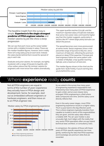
Principal / Lead Engineer

£84,850

Senior Engineer

£70,000

Engineer

£55,500

Graduate / Junior £0

£41,000 £10,000

£20,000 £30,000 £40,000 £50,000 £60,000 £70,000 £80,000 £90,000

The headline insight from the survey is simple. Experience is the single strongest predictor of FPGA engineer salaries and median salaries by job title show a steep progression.

The upper quartile reaches £72,038, and the maximum reported salary of £138,000 indicates that some mid-career roles command far higher pay than the median suggests, particularly in sectors like HFT where large yearly bonuses can distort the picture.

We can see that each move up the career ladder comes with a notable increase in salary. These are the median headline figures, however, and in reality there isn’t a big salary jump at each level. Instead, the salary bands behind them reveal the spread of pay in each role.

The spread becomes even more pronounced at senior levels. Senior engineers show a midpercentile range of £57,000 to £83,700, and a maximum of £250,000, reflecting the premium placed on deep FPGA expertise. Principal and lead engineers follow the same pattern with a median of £84,850, a top quartile reaching £98,250, and a maximum of £220,000.

Graduate and junior salaries, for example, are tightly clustered, with a range of £33,500 to £44,675, with a few outliers above that. By contrast, salaries for engineers with more know-how widens dramatically.

The median figures shown in the chart are the guide here. Quite frankly, if you’re earning less, you’re behind the curve.

Where experience really counts Not all FPGA engineers are equal in terms of the number of years’ experience they actually have in FPGA design and development. Some, for example, start out as embedded software engineers or hardware engineers, and then move on to an FPGA engineer role.

So we asked in the survey how many years of engineering experience respondents had, followed by how many years of FPGA experience to gain a total, and an even clearer story emerged. FPGA engineering is a field where skills compound over time, and the salary curve directly reflects that. Even in the early career stages, more FPGA engineering experience results in a higher salary. The 6–9 year band is the big inflection point. This is where engineers typically transition from capable to trusted in terms of the responsibilities they are given, and the salary data reflects a notable shift. The 30+ year median is also unusually high, but it aligns with the reality that very senior FPGA specialists often occupy hybrid technical-lead, architect, or consultancy roles.

Median salary by FPGA engineering experience

Years of experience

30+ 20–29 15–19 10–14 6–9 3–5 0–2 £0

£20,000

£40,000

£60,000 £80,000 £100,000 £120,000

Less FPGA engineering experience More FPGA engineering experience

In comparison, the salaries of those with fewer years of FPGA-specific experience rise more gently, reinforcing the idea that FPGA expertise and knowledge are premium skills that are rewarded.

The results of the UK FPGA Engineer Salary Survey 2026

Median salary by job title

30+

Total engineering years

The results of the UK FPGA Engineer Salary Survey 2026

Job-change intention by experience

20–29 15–19 10–14 6–9 3–5 0–2 0%

10%

20%

30%

Yes

40%

50%

Not sure

60%

70%

80%

90%

100%

The 7-year itch One of the most interesting patterns in the survey is the mid-career restlessness that appears around the 6–9 year mark. The same mark where we see a jump in the median salary.

A glimpse across the pond

When we looked at whether respondents were considering changing jobs in the next 12 months, a pie chart (if we had one) would show three fairly equal slices for ‘Yes’, ‘No’, and ‘Not sure’. When we overlayed years of experience, the spike at 6–9 years was unmistakable. Nearly half of FPGA engineers are considering moving on. Don’t shoot the messenger.

We wanted to compare apples with apples in the salary survey, so we focused on FPGA engineers in the UK. But what if we added oranges as well by looking at the position for FPGA engineers in the US? How does their experience stack up? If we look across the Atlantic, salary data can be found in the usual mixed bag of sources, each with different methodologies and approaches. There is one source, ShawSilicon.ai, however, that I like because it was founded by an FPGA engineer, for FPGA engineers. Sounds familiar…

The big question is why, and it’s probably because this is the point where engineers have enough experience to be highly employable, but may feel constrained by legacy projects, slow promotion paths or limited architectural influence. It’s also the stage where many companies struggle with retention, not because the work is uninteresting, but because the market is willing to pay for experienced mid-career FPGA talent.

Its FPGA Engineer Salary Guide compiles data from all of those public sources into one place for one simple reason. To provide FPGA engineers with a real-time picture of what the salary ranges are for different positions. There is no gain other than to provide information. Which also sounds familiar.

The takeaway here is perhaps uncomfortable. FPGA engineers at this point need to be rewarded, either with projects that engage and enthuse them, or with the more practical resolution: money.

The median FPGA engineer salaries from the Guide, when it was last updated on 11 July 2026, also have a very similar pattern:

US median salary by job title Principal / Lead Engineer

$250,000

Senior Engineer

$190,000

Engineer

$145,000

Graduate / Junior -$25,000

$102,500 $25,000

$75,000

$125,000

$175,000

$225,000

£275,000

$ They show that US FPGA engineers follow that familiar experience-driven trajectory. Junior roles sit in the lower band, mid-career engineers see a sharp uplift as they take on more responsibility, and senior or principal engineers command a wide and higher salary range.

$ $

FPGA Design made easier. With Livt. ®

Entry-level roles typically start around $85,000 to $120,000, mid-career engineers rise into the $120,000 to $170,000 range, and senior or principal engineers frequently earn $200,000 to $300,000+ depending on sector and responsibility. While the numbers differ, FPGA expertise compounds over time, and the market rewards it once again. The Guide also provides a lot of other useful information for FPGA engineers in the US and you can find it at https://shawsilicon.ai/blog/fpga-engineer-salaryguide-2026/. I did, by the way, spend a lot of time trying to add lemons and limes to the mix as well by looking at EU and AsiaPacific salaries, but the data is so fragmented it was not possible. Apologies.

k Higher-level language k Reusable libraries k Package management k CI/CD tooling k Vendor integration k Development platform

What this means for engineers For new FPGA engineers, the message is encouraging. When starting out, you can look forward to a steep salary trajectory and a midcareer uplift. FPGA engineering remains one of the few technical disciplines where deep expertise is consistently rewarded. For mid-career engineers, the data reflects strong bargaining power. The 6–9 year band is where salaries accelerate and opportunities broaden. And for senior engineers and principals, the data confirms what many already know. Experience is scarce, and companies are willing to pay for it.

more Learn ® at ivt about L m livt o c . s r o t a ecceler

eccelerators.com

t g h n e i l s

o op

clo

PARTNER CONTENT

How AMD Vitis HIL validates real-world execution smarter and f a s t e r Adam Taylor, Founder, Adiuvo Engineering

Simulation used to be the final word in FPGA functional verification. It proved a design was functionally correct before hardware entered the picture. That was then. Modern FPGA systems are complex, and functional simulation can take considerable real time to simulate a few hundred microseconds, which for many applications is just the start of the simulation.

AMD Vitis™ Hardware in the Loop (Vitis HIL) closes that gap by running a design at full speed on real hardware, with the rest of the system in a controllable software model providing stimulus and analyzing results. It exposes performance issues and timing mismatches, and by running in near realtime, reduces simulation time significantly, enabling more scenarios to be applied. Modern workflows have made Vitis HIL practical. Automated board control, Python™or MATLAB® -driven verification, continuous integration pipelines, and affordable development hardware have turned it into a routine verification stage. For FPGA engineers, the rise of Vitis HIL isn’t about replacing simulation. It’s the logical next step in verifying designs that have increased in complexity. As a prototyping methodology running on the device itself, Vitis HIL provides verification between the software simulation stage and full hardware testing. In Python, for example, it keeps your testbench exactly as is, but instead of simulating the design in software, it streams data to and from a physical evaluation board. The testbench sends the stimulus, the hardware executes the full heterogeneous design, and results come back to your host for analysis. This results in a substantial increase in verification performance. By running the design on the target hardware, teams can execute workloads far faster than software or RTL simulation, allowing an increased number of test vectors to be exercised in shorter timeframes. Vitis HIL also enables the execution of design modules or subsystems, providing early confidence in functional correctness and initial performance behavior. This happens all before the complete system is tested on the hardware.

l o op

Bringing into the

With DSP and ML workloads increasing, FPGA engineers are now facing verification challenges that logic alone cannot model accurately. Vitis HIL becomes far more powerful when the device includes hardened compute subsystems capable of running real workloads at silicon speed. One current example of this approach is the AMD Versal™ AI Engine architecture, a grid of SIMD vector processors with local memory and a streaming interconnect. Running AI or DSP kernels on this fabric during Vitis HIL exposes integration of AI Engine / programmable logic (PL) on hardware earlier in the development process, when results of the co-simulation can be verified on hardware across a longer run time. Versal AI Engines feature up to 472 VLIW SIMD vector processors, which deliver tens of tera‑operations per second (TOPS) of hardened purpose-built compute for AI and DSP workloads such as machine learning inference, beamforming, FFTs, and FIR filtering. Highspeed AXI streaming interconnects move data tile-totile on chip, so the engines stay fed at full rate without memory round trips. Dedicated local memory next to each tile keeps operands close, cutting latency and power while sustaining throughput. And because the array and its interconnect are hardened silicon, engineers can avoid timing‑closure challenges and simply program the engines in C++. As a result, AI Engines raise the amount of DSP compute that can be delivered per device compared to programmable-logic-only approaches. Because each AI Engine tile is a vector processor optimized for DSP math, engineers can scale performance by adding tiles rather than stitching together large numbers of DSP blocks and control logic in the PL. This translates directly to PL resource savings. By moving vectorized DSP kernels into AI Engines, significant LUT and flip-flop resources are freed up in the programmable logic. That PL can then be used where it’s most effective: data movement, reordering, control, and system integration. This approach can also deliver lower dynamic power compared to equivalent DSP implementations in general-purpose programmable logic, because the AI Engines are optimized for accelerated vector computing, streaming data flow, and local memory access.

How AMD Vitis HIL valides real-world execution smarter and faster

It gets more challenging when we consider that many FPGA designs include deep DSP pipelines, multi-gigabit interfaces, embedded processors, and even mixedsignal front-ends. Some of these aspects are hard to verify completely in simulation. And as designs grow even more complex, the challenges of functional verification continue to plague developers.

How AMD Vitis HIL valides real-world execution smarter and faster

The key idea is that high-performance vectorizable DSP functions such as filter banks, DFTs, and other math-heavy kernels are best suited for AI Engines. These functions benefit directly from the SIMD vector architecture, local memory, and streaming data flow of the AI Engine array, allowing them to scale efficiently across tiles. On the other hand, data movement and data reordering functions like input permutes, output permutes, cyclic shifts, and DMA stream handling are typically better suited for programmable logic. Vitis functional simulation verifies this partitioning before hardware, automatically creating the necessary connections, and compiles AI Engine graphs and Vitis HLS kernels when required. The flow provides high simulation speeds, enabling millions of vectors to be exercised and metrics to be evaluated in a closed-loop environment. Once functional behavior has been verified in simulation, Vitis HIL then validates the full heterogeneous design on real silicon. It keeps your Python testbench exactly as is, but instead of simulating the design in software, it streams data to and from a physical Versal evaluation board, in this case the AMD Versal AI Core Series VCK190 Evaluation Kit. This delivers at speed execution, real-world memory and interconnect behavior, and early confidence in functional correctness. Notably, for large heterogeneous designs, Vitis HIL removes the multi‑hour or multi‑day wait associated with deep software simulation. Engineers can now validate the same workloads on hardware in minutes, enabling rapid iteration, faster bug discovery, and the ability to explore more test scenarios than would be practical in software simulation alone. It also provides real hardware behavior with the productivity of a highlevel Python test environment. As a result, Vitis functional simulation lets you verify design elements quickly in Python before touching hardware. Co-simulation then validates AI Engine/ PL interaction at the RTL level, after which Vitis HIL improves simulation accuracy by validating your full heterogeneous design on real silicon, offering a complete and efficient verification strategy for AI Enginebased systems.

Turning

theo

With these compute, resource, and power advantages established, the architectural question becomes how the system is partitioned between the AI Engines and the programmable logic.

into practice

Talking about how Vitis HIL gives us real-world results on real silicon is one thing. But what about a real-world example? What do you need and how do you do it? The pattern is the same for any Vitis HIL workflow. You prepare a hardware-ready design, deploy it to a board, start a hardware server or control process, and run a host-side testbench that streams stimuli and collects results. This pattern is exactly what the Vitis subsystem flow follows. Using AMD Vitis software as an example, the Vitis HIL flow is built on a server-host model, where a Python script runs on the host PC and communicates with the Versal board over a standard interface. At the hardware level, a supported FPGA evaluation board is required with a Vitis HIL runtime environment. In the AMD flow, this is a Versal board such as the VCK190, booted from an SD card image generated by using the hil_gen command provided in the Vitis HIL examples. Using this command allows us to define the target VSS, platform, SDK, and RootFS. This results in an image that includes the boot files and the hardware server used for Vitis HIL. On the design side, you then work with a Vitis subsystem. The following example is based around a standard channelizer AI Engine demo application, with a Python framework using Vitis HIL, although any suitable subsystem can be used. Underneath this is the Vitis subsystem with the device under test (DUT), exported as a VSS and ready to go. On the host side, you use the channelizer Python example and the Vitis HIL host script, making sure you set the right IP address for your board in the file.host script, making sure you set the right IP address for your board in the file.

Once it’s up, execute the Python host script to initiate the test sequence. You will see it start running, generating diagrams as it goes, and reporting the Vitis HIL processing throughput, with the channel 1, 2, 5 outputs displayed as the design runs on the board.

Together, the SD card image, the VCK190 board, the Vitis subsystem, and the Python framework form the complete setup for running Vitis HIL with the Vitis software.

1 2

Start with a Vitis subsystem

The Vitis HIL flow begins with a Vitis subsystem packaged as a VSS. It contains the DUT along with the AI Engine design and HLS blocks.

Generate the hardware-ready design

To build the Vitis HIL design, you take the VSS and generate a hardware‑ready version of the subsystem. This build step creates the top‑level design that exposes Ethernet interfaces for streaming data to and from the DUT and for controlling the core. Most Vitis HIL toolchains provide a build step that assembles the hardware‑ready design and supporting runtime files. In Vitis software, you can do this relatively simply by leveraging the hil_gen command, which will generate the Vitis HIL DUT directory as it runs. The hil_gen command builds a full design around the VSS, adding the Ethernet interfaces and producing the boot image, boot bin, and hardware server. This results in an SD card image with your Vitis subsystem on it.

3 4

Boot the board and start the Vitis HIL server

The next step is to deploy the generated SD card image to the target evaluation board (Vitis HIL currently supports the VCK190 and the Versal AI Edge Series VEK280 boards). After booting the system and logging in with root privileges, navigate to the /run/media/mmcblk… partition where you will find the boot image, the boot bin, and the hardware server. Start the hardware server on the board, and it waits for the PC client. (Note that the board boots up in Linux®.)

Run the Python Vitis HIL host

With the hardware server running on the VCK190 board, the next step is to navigate to the channelizer Python example directory. This is what Python uses to run through the Vitis HIL host. Before launching the host script, hardware_in_ the_loop.py, update the target IP address field to match the board’s network configuration.

Observe real hardware behavior

During execution, you will see the wideband signals stream to the target, where the AI Engine array performs channelization in hardware using the AI Engine on the data. You’ll see the input, you’ll see data being reported over on the server, and you’ll see the results coming back to the PC client. The design processing data runs continuously on the board, with results streamed back to the host in real-time. Running the design on hardware exposes real timing, buffering, and throughput behavior that simulation cannot show.

Fit Vitis HIL into the full verification flow

What you’ve seen is how you can use Vitis functional simulation to accelerate algorithm development. Once you’re happy with that, you can run RTL simulation in the wider simulation to make sure everything is working as required. If you want to do some tweaking, you can open the Vitis analyzer to see what you can do with the AI Engines. Finally, you can take your Vitis subsystem and use the Vitis HIL capability to create a solution that drops in the VSS and allows you to simulate it and run it on the hardware. You can use either Python or MATLAB, depending on your preferred environment. The wider flow includes Vivado co-simulation with the AI Engines and algorithm adjustments in Vitis Analyzer before moving to Vitis HIL.

WHY YOU SHOULD

BUILD

fa st

and

faster Reducing engineering uncertainty through simulation, prototyping, and continuous verification Stephen V. Chavez, Principal Technical Product Marketing Manager, Siemens EDA, and Chairman, PCEA

Every FPGA project begins with uncertainty. Before the first line of RTL is written, engineers make assumptions about architecture, interfaces, clocking strategies, timing requirements, memory behavior, and system integration. These assumptions are necessary because engineering decisions must often be made before every variable is known. However, assumptions also introduce risk. The challenge is not that assumptions exist; every complex engineering effort depends on them. The challenge is identifying which assumptions are incorrect before they become expensive hardware problems.

Failure is never the objective: 20

The most successful engineering teams are not the ones that make the fewest mistakes, it’s those that discover incorrect assumptions earlier than everyone else. They understand that simulation, timing analysis, hardware prototyping, design reviews, and collaboration across engineering disciplines are not simply project milestones. They are tools for continuously reducing uncertainty throughout the development process. This philosophy is summarized by the phrase build fast and break things faster. While the expression captures the importance of experimentation and iteration, it can also be misunderstood. In engineering, failure is never the objective. Learning is. Every unexpected simulation result, every prototype issue uncovered early, and every design review that challenges an architectural decision provides valuable information while changes are still inexpensive. The faster a team replaces assumptions with evidence, the more predictable the project becomes. Engineering is not the process of proving that we were right from the beginning. It is the disciplined practice of challenging our assumptions until confidence replaces uncertainty.

The assumption reduction cycle

I often think of this process as an assumption reduction cycle. Every meaningful engineering activity should answer four fundamental questions:

What assumption are we making? What uncertainty remains?

How can we challenge it?

What did we learn? This mindset changes how engineers approach FPGA development. Instead of viewing verification as a final checkpoint before release, it becomes a continuous process of discovery. Simulation challenges assumptions about functionality. Timing analysis challenges assumptions about performance. Prototyping challenges assumptions about hardware behavior. System-level collaboration challenges assumptions about integration. Together, these activities form a continuous learning process that allows engineering teams to make decisions based on evidence.

learning is 21

Why you should build fast and break things faster

Over the course of my career developing and reviewing complex electronic systems, one lesson has become increasingly clear:

Why you should build fast and break things faster

Simulation is about

discovery , not confirmation One of the most common assumptions in FPGA development is that a passing simulation proves the design is correct. While simulation is an essential part of every successful FPGA project, its value is often misunderstood. Simulation does not prove that a design will work under every possible condition. It proves that the design behaved correctly under the conditions that were tested. The difference is significant. Experienced FPGA engineers understand that simulation is not simply a mechanism for confirming expected behavior. It is a tool for discovering unexpected behavior before it reaches hardware. The most valuable simulations are often the ones that expose weaknesses in the design approach, reveal misunderstood requirements, or uncover corner cases that were never considered during initial development.

A strong verification environment intentionally challenges the design. It explores boundary conditions, unexpected sequences, invalid inputs, and operating conditions that may rarely occur but create serious failures when they do. Modern verification methodologies, including constrained-random testing, functional coverage, assertions, and automated regression environments, provide powerful capabilities for improving confidence. However, these tools are only effective when they are built around meaningful engineering questions. The important question is not Did my simulation pass? The better question is What assumptions did this simulation validate, and what assumptions remain untested? This distinction matters because many FPGA failures are not caused by incorrect logic. They are caused by conditions that were never considered.

Every problem discovered in simulation is one less suprise waiting in the laboratory

Timing closure begins with architecture

Clock Domain Crossing (CDC) is a common example. A design may simulate correctly and operate successfully during initial testing while still containing vulnerabilities caused by improper synchronization between independent clock domains. These failures can appear random because they depend on timing relationships that may rarely occur. In reality, the failure is not random. It is the result of an assumption that was never fully challenged. Reset architecture creates similar challenges. Reset logic is often treated as a simple implementation detail, yet incorrect reset sequencing remains one of the most difficult problems to diagnose during hardware bring-up. Understanding how different subsystems initialize and transition into a known operating state requires careful consideration early in the architecture phase. Vendor-provided IP introduces another common assumption: that proven IP requires minimal verification. While reusable IP accelerates development, it does not eliminate engineering responsibility. Configuration choices, interface requirements, timing behavior, and system interactions still require validation. Reuse accelerates development. Verification creates confidence. The two are not interchangeable. The greatest value of simulation is not proving that a design works under ideal conditions. Its greatest value is revealing where the design does not behave as expected while engineers still have the flexibility to make changes. Every problem discovered in simulation is one less surprise waiting in the laboratory.

Another common assumption in FPGA development is that timing closure is primarily an implementation problem. Teams sometimes prioritize functionality first, assuming performance optimization can happen later during synthesis and place-and-route. The reality is that timing performance is often determined much earlier. Architecture decisions involving pipeline depth, clocking strategy, data flow, resource allocation, and logic partitioning directly influence whether the final design can achieve its performance objectives. Once these decisions become embedded in the implementation, correcting timing issues may require significant redesign rather than optimization. Timing closure does not begin during implementation. It begins during architecture. CDC remains one of the most persistent examples. Modern FPGA systems often contain multiple clock domains operating independently to support different functions. Moving information between those domains requires careful synchronization, clear timing assumptions, and an understanding of metastability behavior. A design may appear functional while still containing a fundamental CDC weakness. These issues often remain hidden until specific timing relationships expose them, making them among the most difficult failures to diagnose. Resource utilization creates another challenge. A design that consumes nearly all available FPGA resources may function correctly today but leave little margin for future enhancements, bug fixes, or changing requirements. Successful FPGA teams understand that margin is not wasted capacity. It is engineering insurance. Timing analysis should therefore not be viewed as a final approval step. It should be a continuous engineering activity that informs decisions throughout development. The teams that consistently achieve first-pass hardware success are not successful because they solve timing problems at the end. They succeed because they challenge timing assumptions from the beginning.

Why you should build fast and break things faster

Early prototyping accelerates learning Another assumption that frequently impacts FPGA projects is the belief that hardware should not be evaluated until the design is nearly complete. The reasoning is understandable. Teams want to maximize efficiency by completing functionality before committing time to hardware validation. However, delaying hardware interaction often delays the very learning that can make the project successful. Simulation remains essential, but it cannot perfectly represent every characteristic of a physical system. Real hardware introduces variables that are difficult to model completely, including clock quality, power sequencing, external device behavior, thermal effects, boardlevel interactions, and firmware dependencies. The laboratory should not be viewed as the place where a completed design is finally judged. It should be viewed as an extension of the engineering learning process. The most effective FPGA teams validate capabilities incrementally. They use early prototypes to answer critical engineering questions while the design is still flexible enough to change. Can the memory interface initialize reliably? Do high-speed interfaces maintain adequate margin? Are external devices communicating correctly? Does the system transition properly through power-up and reset? Each answer reduces uncertainty. An early prototype does not need to represent the final product. Its purpose is to accelerate learning.

FPGAs do not exist in isolation One of the most important assumptions to challenge in modern electronic design is that FPGA development can occur independently from the surrounding hardware. Although the FPGA may represent the processing core of a system, it does not operate in isolation. Its performance depends on the electrical environment in which it exists. A design can have correct RTL, successful simulation results, and acceptable timing reports, yet still fail once integrated into the complete system. The reason is simple: the FPGA is only one component in a larger electronic ecosystem. High-speed memory interfaces demonstrate this challenge. Successful operation depends not only on FPGA configuration and controller logic but also on PCB topology, routing, impedance control, return paths, and power delivery. The same relationship exists with high-speed serial links, clock distribution networks, and power integrity. The most expensive design problems rarely occur inside the FPGA or the PCB independently. They occur where the two meet. This is why concurrent engineering has become increasingly important. FPGA designers, PCB designers, signal integrity engineers, and system architects must collaborate earlier in the development process. A pin assignment optimized only for RTL convenience may create unnecessary PCB complexity. A PCB design created without understanding FPGA timing requirements may limit system performance before layout begins. Successful engineering organizations recognize that integration problems are often created long before integration begins.

The objective is not to build a perfect first prototype. The objective is to build enough of the system to learn what needs to improve.

Verification is a continuous engineering discipline Verification is often treated as the final stage before release. Modern electronic systems are too complex for that approach. Verification must become a continuous engineering discipline. Every design change introduces the possibility of unintended consequences. A timing improvement may affect resource utilization. A new feature may impact existing functionality. A subsystem modification may create unexpected behavior elsewhere. Mature FPGA organizations address this challenge through automated regression testing, continuous integration, assertions, coverage analysis, and structured design reviews. Verification should also extend beyond functional behavior. Timing analysis validates performance assumptions. CDC analysis validates clock-domain assumptions. Power estimation validates energy assumptions. Hardware validation validates system assumptions. Together, these activities create confidence that the final product will behave as intended. The purpose of verification is not simply to find defects. It is to continuously replace uncertainty with evidence.

Ten assumptions worth challenging early 1.

A passing simulation proves the design is correct Simulation validates what has been tested, not every possible operating condition.

2. Timing closure can wait until implementation

Performance limitations are often created by earlier architectural decisions.

3. Clock domain crossings are safe because the design appears functional CDC issues may remain hidden until rare timing conditions occur.

4. Reset behavior is straightforward

Reset architecture deserves the same attention as any other critical function.

5. Vendor IP eliminates verification responsibility Reusable IP still requires system-level validation.

6. Functional testing covers all meaningful scenarios

Corner cases often reveal the most important failures.

FPGA performance can be optimized independently of PCB design Physical implementation directly influences system behavior.

8. Integration problems are created during

integration Many failures originate from earlier assumptions.

9. Hardware prototypes should wait until the design is complete Early prototypes accelerate learning.

10. Verification is a project milestone

Confidence must be built continuously throughout development.

Why you should build fast and break things faster

Engineering

confidence through

continuous learning The phrase build fast and break things faster has gained popularity because it encourages experimentation and iteration. Within FPGA development, however, its meaning extends beyond simply moving quickly.

The goal is not to fail more often. The goal is to learn faster. Every simulation that reveals an unexpected behavior provides insight before hardware exists. Every prototype that exposes an interface issue provides an opportunity to improve the design before production. Every engineering discussion that challenges an assumption reduces the possibility of discovering that same issue during the most expensive phase of development. After decades of developing and reviewing complex electronic systems, one observation continues to stand out. The strongest engineering teams are not successful because they avoid mistakes altogether. They are successful because they create deliberate opportunities to discover mistakes while they are still inexpensive to correct. Simulation, timing analysis, prototyping, verification, and collaboration across engineering disciplines all serve the same purpose: replacing assumptions with evidence. Technology will continue to evolve. FPGA devices will become faster, systems will become more complex, and product requirements will continue to increase

Yet one engineering principle will remain constant:

successful teams are those that reduce uncertainty as fast as the project introduces it. That is the true meaning behind building fast and breaking things faster. It is not a philosophy of failure. It is a philosophy of learning. And in engineering, the teams that learn the fastest are usually the teams that deliver the most reliable products.

Robotics Needs Determinism. Not Just Compute. Power-Efficient FPGA Platforms for Deterministic Control, Embedded AI and Sensor Connectivity. Humanoid Robotics Run parallel motor-control loops, synchronize joints and sensors over Ethernet/TSN, and scale to high-DoF systems. PolarFire® FPGAs support real-time control loops as fast as 1 µs.

VectorBlox™ Accelerator SDK 3.0 Add efficient AI inference without GPU-level power. Sparsity and advanced compression improve throughput, reduce memory requirements and enable up to 2X more AI performance from the same FPGA resources.

PolarFire Ethernet Sensor Bridge Connect high-speed sensors to NVIDIA Orin™/Jetson™ and Holoscan AI pipelines with deterministic Ethernet transport. Rev. 2.0 supports up to four MIPI CSI-2 cameras in a 60% smaller form factor for robotics, machine vision and edge AI.

Build robots that move, sense and respond in real time with PolarFire FPGAs and SoCs

The Microchip name and logo and the Microchip logo are registered trademarks of Microchip Technology Incorporated in the U.S.A. and other countries. All other trademarks are the property of their registered owners. © 2026 Microchip Technology Inc. All rights reserved.

Learn more: microchip.com/PolarFire

FPGA strategies for PCB layouts:

Decoupling FPGAs from their BGA restraints Tomas Chester, Hardware Designer and Founder, Chester Electronic Design With FPGAs evolving toward smaller, tighter BGA packages, PCB breakout strategies are becoming more complex. As physical silicon sizes decrease, operational speeds increase, which has the direct knock-on effect of driving up transient current demands. This escalation in power integrity complexity also occurs across a massive frequency spectrum. Due to FPGA capabilities ranging from high-power core logic to high-speed general-purpose I/O and specialized serial transceivers, the power delivery network must support transient power consumption extending from DC all the way into the gigahertz range. All of this calls for a different approach to our decoupling strategies for FPGA BGAs, with multiple layout techniques to minimize loop inductance, along with designs that maximize decoupling density and capacitor availability within highly restricted footprints.

While both discrete components can be explicitly selected and placed, we can also create an even faster, albeit smaller, highfrequency storage element within the layers of the circuit board. In these inter-planar capacitors, the structure is formed by closely coupling power and ground planes within the PCB stackup, resulting in a planar capacitor that can respond in the early nanoseconds to handle noise within the 100 MHz to 1 GHz range.

Notably, not all capacitors are created equal. Bulk capacitors store massive amounts of energy and are used to refill the smaller storage elements located closer to the operating devices, operating in the sub-100 kHz range. Localized ceramic capacitors of varying values, meanwhile, provide immediate local current stores that can respond in the 100 kHz to 100 MHz range.

For transient speeds surpassing this threshold, we must rely on the capacitance built directly into the FPGA silicon and its on-die termination to handle the ultra-high frequency power distribution. This relationship is visualized in Figure 1, which maps frequency spectrums against the response times of various capacitor types and locations.

Fig 1. Frequency spectrum vs decoupling response time

When planning the PCB layout for a design, the focus should be on what we can directly control, like the physical placement of localized ceramics and bulk capacitors, and the deliberate creation of internal planar capacitance if the board stackup allows. It is critical at this point to consider these three elements as a tightly linked chain. The high-frequency planar capacitance is refilled by the localized ceramic capacitors, which in turn are replenished by the bulk capacitance, which itself is restored by the onboard or offboard power supplies. If a single link in this chain is poorly designed, it can trigger a cascading failure that starves the FPGA during periods of high utilization. Crucially, capacitors possess a spatial response area. A capacitor placed under or near an FPGA, while directly tied to a specific pin, will also naturally support neighboring pins within its respective frequency response range. A stylized graphical representation of this can be seen in Figure 2. Although the full capacitance may not be entirely available to those adjacent pins due to the increased trace and plane distance, capacitors do not exist in total isolation. When applied to a massive component like multi-hundred or thousand-pin BGA FPGAs, this phenomenon behaves like ripples in a pond. Dropping a single water droplet creates predictable waves, but introducing multiple rocks results in complex wave reflections and interactions at many locations. I find that imagining current flow as fluid dynamics is helpful. While not a perfect representation, it provides a highly effective mental model for optimizing a physical layout.

Fig 3. Double-wide routing channels and possible capacitor BGA placements

Fig 2. Capacitor response range dropoff

Capacitors placement within the BGA breakout pattern Another major factor influencing power integrity is the via breakout pattern used to escape the FPGA’s BGA grid. While via breakout choices directly assist with the connectivity and overall solvability of the FPGA, the specific strategy utilized can simultaneously act as a bottleneck for the current flowing through internal power plane layers, and as a minefield with respect to the localized placement of the decoupling capacitor network. If we start by examining a 1.0mm pitch BGA, placing 0402 capacitors directly onto the opposite-side via grid is highly feasible. Depending upon the specific land pattern geometries, 0603 capacitors can typically also be placed within the via grid, provided that viain-pad plated-over (VIPPO) techniques are allowed, or appropriate spacing occurs thanks to component rotation. However, integrating larger components like 0805, 1206, or 1210 capacitors directly within the standard breakout grid is impossible if every BGA pin is broken out without any additional spacing. The exception to this rule is when a quadrant breakout is utilized, as can be seen in Figure 3. By clearing the central via row and column, a quadrant breakout leaves a double-wide routing channel, enabling large- to mid-range ceramic capacitors to be placed either directly over the vias, assuming via-in-pad is allowed, or to be nested comfortably within this channel using short trace routing lengths to minimize parasitic inductance. This allows for minor, high-frequency ceramic bulk capacitance to be added closer to the device, while larger tantalum, aluminum, or polymer bulk capacitors remain outside the local perimeter.

FPGA strategies for PCB layouts: Decoupling FPGAs from their BGA constraints

Optimizing the power delivery chain

FPGA strategies for PCB layouts: Decoupling FPGAs from their BGA constraints

The importance of loops

When moving to smaller BGA pitches, our selection of available capacitor package sizes is drastically compressed. On a 0.8mm pitch grid, 0402 capacitors are easily placed, but moving up to an 0603 package forces the capacitor to skip or completely mask a via underneath it. The larger 1206 or 1210 footprints cannot be utilized within the grid at all, though 0805 capacitors can still fit within the quadrant channels if they are available.

Semiconductor manufacturers typically position high-speed transceivers near the outer perimeter of the BGA package. This thoughtful pin assignment simplifies both the high-speed escape routing and the core power decoupling placement, though decoupling and power delivery within these transceiver PCB layout sections can still present unique challenges.

Stepping the BGA pitch down further requires switching from 0805s to 0603s within the escape channels, forcing creative layout arrangements of 0402s or a complete transition to ultra-small 0201 packages within 0.65mm and 0.5mm pitch grids. Once a design hits a 0.5mm pitch or below, the use of microscopic 01005 capacitors often becomes an absolute requirement.

Beyond physical component sizing, loop inductance is critical to power integrity, so we need to understand how they are connected. Loop inductance represents the total geometric path that a high-speed current transient must traverse as it exits the decoupling capacitor, travels to the FPGA, and returns along the ground path.

In high-density layouts, designers can leverage naturally occurring via void areas. These spaces can then be intentionally modified, creating larger, deliberate gaps to place larger package sizes right inside the tight via fields necessitated by the FPGA BGA component. Furthermore, if the breakout utilizes more complex HDI structures like blind or buried microvias, this will open up the opposite side of the board, granting freedom for capacitor placement since the through-board via barrels are eliminated.

This loop is comprised of three primary physical elements that are doubled by the nature of the round-trip return path: the distance from the capacitor pad to the via within the BGA via grid; the vertical height of the via barrel itself; and the distance from that same via to the FPGA pad. Because a via is inherently an inductive structure in a PCB layout, systematically shrinking the loop area, and specifically minimizing the active via height, is of critical importance for power integrity.

However, while HDI features such as blind and buried microvias assist with component placement, the introduction of back-drilling can do the exact opposite, drastically increasing layout complexity. Because back-drilling mechanically reams out the unused stubs of through-hole vias to protect signal integrity, it creates large physical void zones and keep-outs on the opposite side of the board where capacitors would traditionally sit. Depending upon the specific layers that are back-drilled, this process can quickly turn internal power planes into Swiss cheese.

Figure 4 illustrates several side-by-side examples of capacitor-to-via routing configurations for capacitors placed back-to-back with the FPGA. These examples utilize guidelines derived from the AMD Architecture PCB Design User Guides (UG483 and UG583). The configurations include a long trace to a via; a short trace to a via; a dual-via per pad layout with short and wide traces; and finally a full via-in-pad plated-over solution.

Fig 4. Capacitor land pattern and mounting examples (worst to best, left to right)

The first three examples can typically be processed using standard, low-cost fabrication methods. The via-in-pad approach, however, may demand additional manufacturing fabrication steps to plug and plate over the holes. These plugging and plating steps, which introduce extra cost and lead time, depend on the operating environment, production volumes, and other design requirements that should be carefully considered. For our example, a standard 1.57mm board thickness is used, making the vertical via barrel identical across all four scenarios. Therefore, the only variable affecting performance is the lateral routing geometry from the capacitor pad to the via and from the via back to the FPGA pad. Reducing this routing distance directly optimizes our power delivery by shrinking the total inductive loop area. In our fluid dynamic mental model, the capacitor is a water tap and the connecting trace is the pipe delivering water to the storage tank, the FPGA. A longer trace increases resistance, delaying supply during a sudden drop in pressure. This shows that a shorter trace is clearly a better solution as power is provided in a more timely manner. The dual-via configuration with wider traces mimics installing two larger-diameter pipes in parallel, drastically increasing the flow rate as compared to a single, narrower pipe. Again, this provides a clear example that the dual-via solution or a wider trace solution is superior to a single, narrower trace. Finally, the via-in-pad structure represents the ideal scenario where the pipe is eliminated entirely, mounting the tap directly onto the tank. Here, though, we must still account for the vertical distance the current travels down the via barrel to reach the opposite side of the PCB.

While these planar cavities only yield capacitance in the picofarad range, they act as an instantaneous firstresponder pool of charge. This localized plane cavity is then continually replenished by the neighboring ceramic decoupling capacitors, which can be placed either directly opposite the BGA or strategically distributed around its perimeter. This layout choice can potentially unlock a cost-effective, single-sided assembly solution, provided that the perimeter capacitor cluster does not create an unroutable escape bottleneck for the surrounding signal lines.

Custom capacitor land patterns for dense BGA fields When dealing with dense BGA packages and highlyutilized FPGAs where every pin must be broken out, we must look for every geometric advantage possible. One such advanced method to enable larger capacitor placement within these tight BGA via fields is the creation of customized land patterns, specifically modifying the geometry of the capacitor terminal pads, as shown in Figure 5. However, it must be emphasized that these are highly specialized solutions; designers must perform their own due diligence based on their specific product environment to ensure these modified footprints comply with any target certification classifications, reliability standards, IPC manufacturing specifications, or environmental requirements. The first custom configuration is an octagonal pad rather than a traditional rectangle or rounded rectangle. This shape is designed to fit within the curved, circular clearance boundaries of the mechanical or laser vias that comprise the BGA breakout grid. By cutting the 45-degree corners of the pad to match the via clearance arcs, we can squeeze a slightly larger capacitor package into an otherwise restricted space.

Leveraging planar capacitance This structural reality introduces a perfect opportunity to leverage internal inter-planar capacitance. By utilizing a planar capacitor, we replicate the benefits of a via-in-pad design while minimizing the effective height of the via barrel. We achieve this by placing our power and ground plane pairs immediately adjacent to one another on the layers closest to the outer surfaces of the PCB, typically Layers 2 (GND) and 3 (PWR).

Fig 5. Capacitor land pattern BGA geometry modifications

FPGA strategies for PCB layouts: Decoupling FPGAs from their BGA constraints

Finally, reverse-geometry low-inductance capacitors can be utilized if they are available in the required values. An example would be substituting a standard 0805 component with an 0508 reversegeometry package. By flipping the terminations to the long sides of the component body, the internal current path is dramatically widened and shortened, drastically reducing the component’s Equivalent Series Inductance (ESL) while perfectly matching the parallel routing channels under a dense BGA.

This modification does introduce a manufacturing trade-off. Altering the pad geometry directly reduces the surface area available for solder paste deposition. Unless stencil apertures are specifically adjusted to compensate, this reduction can result in a starved solder joint, weakening the mechanical bond between the PCB and the capacitor. Consequently, an altered pad geometry may provide a clear advantage for layout solvability, but it can introduce a distinct disadvantage regarding assembly yield and long-term mechanical reliability.

Summary

The second example is a further evolution of the octagonal concept, substituting the 45-degree corner cut with a custom radiused curve. This concave curve matches the exact radius of the adjacent via’s clearance keep-out, maximizing the copper-to-copper gap beyond what a straight angle can achieve. This footprint style is exceptionally specialized, as its geometry is tightly coupled to the combination of BGA pin pitch, via drill diameter, and annular ring size. If any of these fabrication parameters change, the custom-curved land pattern would require an update to meet the shifting fabrication dimensions.

Meeting modern FPGA power delivery requires balancing foundational physics, layout constraints, and custom pad geometries. Ultimately, the power distribution network (PDN) and overall power integrity are of the utmost importance to ensuring smooth, consistent FPGA operation under heavy transient loads. The layout techniques and customized land patterns explored here can be utilized beyond FPGAs, providing a robust framework for any high-density, high-speed component within a design.

The third example shifts from placing a capacitor between four vias to intersecting a via row or column directly, which is often required for larger components. In this layout scenario, the connected power or ground via resides directly within the capacitor’s land pattern pad itself, while the adjacent non-connected vias create an immediate bottleneck.

While electrical physics governs power delivery, layout strategy is only part of the board-level challenge. The next step in this series about advanced PCB design will move from the power delivery grid to the signal lines themselves, examining advanced routing breakout techniques and the unique options that exist once high-speed signals have successfully escaped the BGA package.

To handle this, the capacitor pad is customized with specific relief cutouts, typically on the two short edges of the pad, but in some extreme cases on all four edges, to clear the copper rings of those neighboring, non-connected vias. While highly effective, this technique requires extreme care during manual layout or routing. A non-connected signal via must never become trapped or shorted within an opposing net’s power or ground pad.

This is the third Journal article in a series from Tomas Chester about advanced PCB design. In issue 1, he looked at the strategies for a PCB layout and compares chip‑down FPGA BGAs with SOM‑based designs.

All three of these solutions rely on the aggressive modification of standard footprint geometries. However, several alternative strategies can achieve similar density gains without requiring custom pad fabrication. For instance, utilizing non-standard component rotation by orienting capacitors at arbitrary angles outside the traditional 45 or 90-degree constraints can often slip a component neatly between diagonal via patterns. Alternatively, designers can deliberately share power or ground vias between adjacent decoupling capacitors to save physical space and increase the overall decoupling density within the BGA grid core.

In issue 3, he examined sparse vs dense via breakouts, showing how BGA pitch affects solvability, via technology choices, and the point where HDI becomes unavoidable.

System-in-Package (SiP) Solutions Efinix® system in package solutions combine our FPGA die with memory die into a compact solution. Reducing PCB complexity, speeding time to market, and alleviating memory supply chain headaches

• Low power consumption • SPI ﬂash for conﬁguration and user data • Integrated Flash in a 14x14 mm LQFP package

• Optimized performance, eﬃciency, compact design

• 2nd generation high-speed I/O • Hardened Quad-Core RISC-V Processor • SEU correction and ultra-low

• 15x15 mm package with static power operation integrated LPDDR4x SDRAM • Integrated SPI ﬂash and two • 5.5x5.5 mm package with HyperRAM in a 8x8 mm integrated SPI ﬂash and package HyperRAM

• High-performance data-intensive workloads • Integrated SPI ﬂash and LPDDR4/4x DRAM in 16x16 mm package

Applications

Edge AI

Industrial Automation

Automotive

Machine Vision

Robotics

Medical

Achieve Low Power, High Speed, and Compact Board Designs

Ready to Simplify Your Next Design? Scan to learn more:

www.efinixinc.com

An open-source Mini-ISP: Image Signal Processor for FPGAs Timor Knudsen, Strategic Applications Engineer, AMD Image signal processing is one of the few areas of FPGA development where the results are immediately visible and widely understood. Unlike many FPGA workloads, image pipelines produce outputs that both experts and non-experts can evaluate. An Image Signal Processor (ISP) converts raw sensor data into consumable digital RGB images, typically distinguished as human vision or machine vision. For human vision, the ISP focuses on producing an aesthetic image, often with requirements around style or atmosphere. Machine vision focuses on a specific detection or classification task, which can mean dramatically different or reduced processing. When semiconductor manufacturers harden an ISP into their SoCs, however, they face tough trade-offs. Trim features, and it limits use cases; add flexibility, and cost goes up. For a long time, the mantra has been: What’s good for human vision is good for machine vision. Special machine-vision needs then fall back to general-purpose compute such as a Digital Signal Processor (DSP), Graphics Processing Unit (GPU), or Central Processing Unit (CPU). The issue we need to contend with is that image signal processing requirements vary widely across sensors and applications, yet those ISP trade-offs mean no single ISP can meet every need.

But why do we need an ISP at all in the era of Deep Neural Networks (DNNs)? Can’t we just feed raw sensor data into a DNN and let the network condition it end-to-end? In principle, yes – but there are drawbacks.

How Mini-ISP changes the picture

First, you need to retrain your network on data from your specific sensor, and collecting training data in challenging open-world environments (automotive, robotics, drones) is extraordinarily costly. Second, raw data delivers surprisingly little benefit for many detection and classification tasks. Third, the ISP functions a DNN must learn are mature and wellunderstood. We can implement them directly with far less compute, freeing the DNN to spend its compute budget on the actual task.

While the cost of ISP development is often prohibitive, FPGAs are uniquely positioned for custom ISP. To demonstrate this, I started a personal project two years ago to design a modular ISP specifically for FPGA implementation. The result? Mini-ISP, which has now been released as open-source with the support of AMD.

Demosaicing then converts the CFA raw data into three-channel RGB images by interpolating the missing samples, using the well-established Malvar-He-Cutler (2004) algorithm.

In the Black Level Correction block, sensor pixels generate dark current that varies with process, voltage and temperature (PVT). Optically black pixels serve as the reference for the ‘black’ readout level, which the sensor maps to a digital value that we later need to subtract from the raw data.

After conversion to RGB, the Color Correction Matrix maps the sensor’s RGB into a well-defined color space by multiplying each RGB triple by a Color Correction Matrix (CCM). Many applications need color constancy, so the CCM coefficients can be changed dynamically based on estimated scene illumination color temperature. Lastly, the target color space may need a non-linear tonal curve like a gamma function. The Gamma LUT applies arbitrary curves and combines the operation with bit-width reduction (e.g. 12 bits per channel down to 8 bits). Two more blocks already exist or are planned. High Dynamic Range (HDR) sensor data is often companded to save bandwidth between camera and host, and Decompanding rebuilds the linear data. Camera lenses impact how much light reaches different areas of the sensor (also known as vignetting), and Lens Shading Correction (LSC) corrects this with a radial distortion model.

Fig 1. Block diagram of a Mini-ISP in a typical application, with the MIPI CSI-2 subsystem and Frame Buffer Writer connected.

Mini-ISP: An open-source Image Signal Processor for FPGAs

The Color Gain stage multiplies the raw data by per-channel gain factors. This is to correct the color filter arrays (CFAs) which usually show different sensitivity per color. Green is typically the most sensitive, for example, and white balancing requires that all three channels reach the same digital level for gray and white pixels.

Mini-ISP ships with simulation models, test benches and Verilog RTL, and provides a modular framework that can be extended or customized using modern AI-assisted coding tools. The framework provides building blocks for ISP development, along with reference implementations.

Mini-ISP: An open-source Image Signal Processor for FPGAs

Mini-ISP capabilities Fully Parameterizable

Input bit width from 8-24 bit and beyond Horizontal resolution 1024-8192 pixels and beyond Vertical resolution limited only by frame rate / pixel throughput

High Throughput

1, 2 and 4 Pixel-per-Cycle (PPC) supported 500 MHz pixel clock achievable on some AMD devices Up to 2 GPixel/second

Low Resource Usage

Typically less than 5000 LUTs Typically less than 50 DSP slices Typically less than 20 BRAM

Interfaces

Integrated with Vivado IPI AXI4-Stream Video Interfaces for video in and video out AXI4 Lite Register Interface

Why Mini-ISP is designed this way Mini-ISP follows five core principles. The first is minimal resource usage. Mini-ISP aims to be as small as possible, so it fits even the most resourceconstrained AMD FPGAs. The second is maximum performance. Mini-ISP is fully pipelined, optimized for fast pixel clock, and processes 1, 2 or 4 pixels per cycle. With its specs, even the most demanding video formats such as 8K at 60 frames per second (FPS) can be processed in real time. The third is correctness. That’s not always trivial to define, especially when we approximate certain math functions, as is common in vision. But the output must always match what we intended. Fourth, image quality must be acceptable for most applications, including human vision. But only that: acceptable. A high-quality ISP aiming for outstanding visuals would make different choices, drive resource usage up, and likely conflict with other core principles.

The last principle is being open-source. Users must be able to read, modify and extend the code for their own needs, and ideally be able to contribute back. Mini-ISP follows a develop-in-the-open approach for maximum transparency. Being open also means we can’t use proprietary algorithms. When it comes to ISP algorithm selection, a few processing steps you’d expect in any ISP are deliberately absent from Mini-ISP. Spatial denoising. Algorithms such as BM3D and CNN-based denoising deliver fantastic results – but they’re far too expensive for Mini-ISP. Cheaper options like Wiener filtering, Non-local means (NLM) or rankorder filters with small context windows don’t justify the resources. Temporal denoising is efficient and produces excellent results, but it requires framebuffers, which are out of scope for Mini-ISP. Sharpening or deconvolution. Simple sharpening typically just recovers edges lost in earlier ISP steps such as denoising. The trade-off between sharpening edges and amplifying noise rarely justifies the resources, especially since sharpening also needs a context window. Local Tone Mapping (LTM). HDR images need tone mapping to match the lower dynamic range of displays. Global Tone Mapping (GTM) applies a single curve to the whole frame, while LTM adjusts the curve per local region. LTM can produce great results, but eats huge amounts of FPGA resources to build the local context, often looks unnatural, and can suffer from halo effects and instability across video frames.

Open-source IP development Mini-ISP leans heavily on the open-source RTL ecosystem. Git for source control and Python for algorithm prototyping are industry standard. Self-checking test benches that run on every commit in a Continuous Integration / Continuous Deployment (CI/CD) pipeline are an absolute must, which puts simulation speed front and center.

Verilator

One of the fastest RTL simulators out there is opensource: Verilator. With roots back to 1994, it’s exceptionally mature. It translates the synthesizable subset of Verilog RTL into parallelized C++ code, which is then compiled and executed. Optionally, we can dump signals as VCD files for waveform inspection. Verilator’s raw speed and maturity is why Verilog was chosen for Mini-ISP rather than VHDL – the VHDL ecosystem doesn’t offer a similarly fast open-source solution. Verilator isn’t a full simulator, though, as you can’t build test benches with just the synthesizable subset.

cocotb

That’s where cocotb comes in. cocotb is a co-simulation test bench environment for verifying Verilog RTL in Python. Its backend supports several simulators, and Verilator support has matured rapidly in recent years. The two projects are a perfect match: cocotb implements and orchestrates test benches, while Verilator executes the RTL. Despite the extra build steps, the combined process beats even commercial simulators on speed. Python test benches bring great benefits. The whole Python ecosystem becomes available for generating and validating data, which is especially valuable for image and video processing, where libraries like NumPy and OpenCV make life much easier. Established frameworks such as pytest organize and run our tests, and we use the same environment for the reference implementation and the test benches.

cocotbext-axi

cocotb has an extension mechanism, and one of the most useful extensions for Mini-ISP is Alex Forencich’s cocotbext-axi. It lets cocotb test benches transparently talk to standard AXI interfaces – AXI Stream or AXI memorymapped – reducing complex transactions to a few lines of Python.

Mini-ISP: An open-source Image Signal Processor for FPGAs

How does it all come together? A cocotb pytest test bench can look like these snippets from the black level correction test bench: @cocotb.test() @pytest.mark.sim async def test_blc_basic(dut): tb = TB(dut) tb.set_idle_generator(generator=tb.random_pause) tb.set_backpressure_generator(generator=tb.random_pause) await tb.reset() cfa = np.random.randint(…)

It’s very useful to drive both the AXI Stream source TVALID and the AXI Stream sink TREADY with random sequences, so the AXI Stream logic inside the module sees many different combinations. It also makes sense to fully randomize the NumPy input image to cover a wide range of values. We feed it into the RTL module with a simple loop: tuser = [1] * tb.axis_source.byte_lanes + [0] for y in range(0, h): frame = AxiStreamFrame( pack_buffer( cfa[y, :].astype(np.uint32), int(dut.PIXEL_PER_CYCLE.value), int(dut.PIXEL_BIT_WIDTH.value), ), tuser=tuser, ) await tb.axis_source.send(frame) tuser = 0

Each AxiStreamFrame represents a single image line, and TLAST is asserted automatically on the last transaction. We assert TUSER on the very first transaction to mark the start of frame. pack_buffer packs np.uint32 pixel words into a byte array following the AMD AXI4-Stream Video format. Reading the result is very similar: result = np.zeros((h, w), dtype=np.uint32) for y in range(0, h): frame = await tb.axis_sink.recv() result[y, :] = unpack_buffer( frame.tdata, int(dut.PIXEL_PER_CYCLE.value), int(dut.PIXEL_BIT_WIDTH.value) )

We then check the resulting NumPy frame against a reference implementation with automated pass/fail criteria: blc = BlackLevelCorrection(dut.black_level.value.to_unsigned()) ref = blc.reference(cfa) np.testing.assert_allclose(result.astype(np.uint32), ref.astype(np.uint32), atol=0)

Test parameters such as PIXEL_PER_CYCLE and PIXEL_BIT_WIDTH are automatically swept across valid values, so this single test covers all parameter combinations. Mini-ISP uses uv to manage the Python project. To run pytest, just invoke: $ uv run pytest -m sim -k "blc"

Yosys and pyosys

Resource usage matters at every step of IP development. For immediate feedback, Mini-ISP uses Yosys (Yosys Open SYnthesis Suite) and its Python module pyosys to synthesize the design and extract FPGA resource utilization numbers. The pyosys results are exported as Markdown, then converted into HTML documentation using Zensical. A GitHub Action publishes them to GitHub Pages on every commit, giving us continuous resource monitoring.

VS Code, Docker and Dev Containers

Mini-ISP ships with a development Dockerfile that doubles as a CI/CD image and a VS Code Dev Container. When you open the repository folder, VS Code detects the Dev Container configuration and builds the container, with every Mini-ISP tool and dependency preinstalled. To view Verilator VCD waveform dumps, I highly recommend the Surfer Project VS Code extension.

AI Coding Agents

A fully scripted, instrumented dev environment pays huge dividends with AI agents. Mini-ISP doesn’t yet contain any AIgenerated source code, but the framework lets you implement Verilog RTL modules with help from coding agents. Agents tend to hallucinate and produce good-looking but nonfunctional, unmaintainable code. The key is to give them process descriptions, detailed instructions, and strict guardrails via a dedicated SKILLS.md file, and to force them to use real tests and scripts to validate their output. One workflow that’s worked well mirrors a regular development flow: hand the agent a Python reference implementation, then ask it to produce optimized Verilog RTL. For every change, the agent needs to run the automated test bench to prove the Python reference and the generated Verilog are equivalent. It uses pyosys synthesis results to monitor resource usage. This dramatically shrinks the room for hallucinations and improves the quality of generated Verilog RTL code.

Mini-ISP: An open-source Image Signal Processor for FPGAs

AMD Spartan™ UltraScale+™ FPGA Vision Demo Mini-ISP is part of the SCU200 Vision Targeted Reference Design (TRD). A single AMD Spartan™ UltraScale+ FPGA processes three Raspberry Pi HQ cameras (Arducam) at 12 MP and 40 frames per second, and outputs 4K 60 Hz over HDMI.

The design contains three AMD MIPI CSI-2 Receiver Subsystems, each configured for 4 lanes, 1500 Mbps lane rate, and 4 PPC at the output. One Mini-ISP instance per camera converts the 3840×2160, 40 fps, 12-bit stream to RGB888 at a 300 MHz pixel clock. The total theoretical system pixel bandwidth computes to: NUM_INST * PIXEL_CLOCK * PIXEL_PER_CLOCK =

3 * 300 MHz * 4 = 3.6 GPixel/s. Each Mini-ISP instance uses the following resources in this configuration:

Fig 2. An SCU200 demo setup using an AMD Spartan UltraScale+ and three Raspberry Pi HQ cameras.

LUTs Registers DSP48 BRAM

2373 4714 40 12

Fig 3. A ColorChecker chart with test objects, illuminated at 3000 K color temperature, with an Raspberry Pi HQ camera with Sony IMX477 sensor, 3840×2160, 40 fps output, processed by the Mini-ISP in the same configuration as the SCU200 Vision TRD demo.

Conclusion FPGA IP core development has changed substantially over the last few years. Open-source tools now lead the way in speed, usability and integration. It’s hard to imagine an equally effective workflow built on proprietary tools alone. Mini-ISP rides this ecosystem and aims to lower the barrier for both contributions and similar IP projects. With AI coding agents, there’s a clear path toward dramatically lower development cost for custom ISP solutions. If this ISP development approach sounds interesting, check out the Mini-ISP repository on GitHub. Mini-ISP is licensed under the permissive MIT license and is available at https://github.com/amd/mini-isp.

From Idea to Series Production FPGA & SoC Solutions. Engineered and Manufactured in Germany.

FPGA & SoC Devlopment Custom Hardware Solutions Turnkey Solutions In-House Manufacturing Lifecycle Support

Key Application Areas

Research

Medical

Test & Measurement

Start your next FPGA project

Industrial

trenz-electronic.de

Defence

Why containerization is essential for modern EDA workflows Alper Yazar, Principal Engineer, ASELSAN Most of us protect our source code carefully with version control tools like Git or SVN, but source code on its own doesn’t do much. It only becomes a useful output, like a bitstream, after a tool compiles it. The trouble is that the Electronic Design Automation (EDA) tools we rely on from vendors are heavy, hard to set up, fussy about their dependencies, difficult to scale, and the output can vary.

This is important because we don’t ship our HDL files to a customer; we ship a bitstream, a binary, a piece of firmware. That output is the product of the code and the tool that compiled it. You can write the same Verilog twice, feed it to two different versions of an EDA tool, and nothing guarantees the same bitstream comes out.

We c a n p u t t h i s i d e a i n a s i m p l e f o r m :

output = f(source code, toolchain, ...) The bitstream (the output) is a function of at least two inputs, not one. Other factors (like a place-androute algorithm seed) can change the result too, but these two matter most. Version control takes good care of the first. The second, the toolchain, is the part most of us ignore, and it’s just as important. This matters even more for FPGA work, because these projects live a long time, sometimes decades. Over that lifetime, the last thing you want is to be forced to upgrade your EDA tool. A newer version is not automatically better for an existing design, and nothing guarantees an updated IP core is free of new bugs. Your design didn’t change, yet you’ve taken on risk you never asked for. That’s exactly the trap containers keep you out of.

EDA tools make protecting your toolchain genuinely hard and it starts with dependencies. A typical EDA tool leans on a long list of system packages and specific library versions. Two releases of the same tool may each demand a different version of the very same library, and your Linux distribution can keep only one of them happy at a time. With PetaLinux, for example, each version expects a particular Ubuntu release and matching apt packages, so installing two versions side by side can lead to problems.

What a container looks like Let’s make this concrete. Here’s an example of what it looks like in practice, using Docker and an opensource Linux project, Embedded Box (EBox), as a working example. Imagine we want to package a simple command-line tool that needs a couple of system libraries:

Getting the dependencies right in the first place is hard too. For example, tools like Vivado ship a helper script to pull in the packages they need, but it can be incomplete. You often need to piece the real list together from the official script plus community fixes from forum threads or blog posts, get it running, and years later struggle to remember exactly what you did.

# Start from a known, fixed base image FROM ubuntu:22.04 # Install the system packages our tool needs RUN apt-get update && apt-get install -y \ python3 \ libssl3 \ make

This introduces problems when it comes to reproducibility, and it’s the heart of the matter. A reproducible environment is one you can stand up again next year, on a different machine, and trust to behave exactly as before. Without that, every fresh install is a small gamble, and across a dozen tools and several projects, that gamble becomes the background stress of the whole job.

# Copy our tool into the image COPY my-tool /opt/my-tool # Run this command when the container starts CMD ["/opt/my-tool/run.sh"]

Even if you’ve never seen one before, you can almost read it like plain English. FROM picks a starting point, here a fixed Ubuntu version, so everyone builds on the same foundation. RUN runs commands inside the image, COPY brings our own files in, and CMD says what happens when someone starts the container.

Why containers are a strong choice A container packages an application together with everything it needs to run, so it behaves the same on any machine you start it on. It is not a full virtual machine. Instead of carrying a whole separate operating system, it shares the host’s kernel and keeps only the pieces above it, which makes it small and fast to start.

Ubuntu 22.04 is the base used here, but the host can be a different Linux distribution, or even Windows or macOS. As long as it has a container runtime, the tool runs the same way everywhere, on the same minimal Ubuntu 22.04 with the same packages. The knowledge that used to live in your memory now lives in a file that doesn’t forget.

You describe the environment once, in a plain text file: the libraries, the packages the tool needs, the little tweaks you’d otherwise forget. From then on, anyone can rebuild the exact same environment from that description. The container also carries what is in effect its own operating system layer, so an old tool keeps running on its own foundation no matter how far the host moves on underneath it, which is exactly what protects you from the upgrade trap.

Real EDA tools need a longer recipe, of course. The EBox Dockerfile for Vivado and Vitis 2024.1 runs to over 200 lines and works around several issues that only show up in practice, with comments pointing to the exact AMD articles behind each fix. You do that detective work only once, write it into the Dockerfile, and every build after that gets it right automatically.

Why containerization is essential for modern EDA workflows

A virtual machine could capture an environment too, but it drags a whole guest operating system along, which makes it heavy and slow to automate. Containers start in seconds and also slot naturally into CI/CD pipelines, so for capturing a toolchain and reusing it they’re usually the better fit.

Why EDA Tools are hard to pin down

Why containerization is essentail for modern EDA workflows

Scaling your builds

What you need, and how to use it

A containerized toolchain rebuilds the same way every time, which is exactly what an automated pipeline needs: getting the same result it would on any other machine. The environment stops being a variable you worry about.

Before you can run an EBox image, a few things need to be in place. First, a container engine: Docker or Podman on Linux, which is the smoothest path since EBox is built and tested mainly on Linux.

That leaves scaling. To build many projects at once, you need a pool of build servers, and handmaintained machines hurt here. The old way is to install your tools by hand on each backend machine and connect it as a CI/CD runner. It works, but every machine is a fresh chance to get the dependencies wrong, and when you need five more, you repeat that painful setup five more times.

Second, the tool’s installation files from the vendor. While EBox gives you the recipe, you supply the main ingredient, the installer. You bring the official file you downloaded and EBox handles the rest. These files are not small; current Vivado installers easily pass 100 GB. Third, disk space and time. The image holds a fully installed copy of the tool, so it ends up large too, sometimes over 100 GB, though a configuration file lets you drop device families you don’t need. Building it is a one-time cost that can run an hour or more, but once the image exists, starting it takes only seconds. Plan for fast disk, ideally an SSD.

Containers turn this around. You run generic runners whose only job is to execute containers, and the toolchain rides along inside the container image, so any runner can run any job. Need more capacity? Add another generic runner pointed at the same images. Because the runners are generic, you can even get them as a service from your IT department. Nothing FPGA-specific has to live on their side.

Here’s the typical flow, using the Vivado and Vitis 2024.1 image. First, clone the EBox repository, place the vendor installer in the build directory, and build the image, tagging it with a version so you can tell builds apart:

A self-hosted GitLab runner using the Docker executor does exactly this, it’s free, and it can run in fully offline environments. The reproducibility you gained on your laptop now holds across the whole build farm, because it’s the very same image everywhere.

sudo docker build -t vivado:2024.1 . Building is a one-line command, so take your coffee and relax. Once it builds, you can keep the image local or push it to a registry (such as the GitLab Container Registry), so your CI runners can pull the same image your laptop uses. To check it works, run it headless and ask the tool for its version:

EBox in practice

sudo docker run --rm -it --user ebox vivado:2024.1

EBox isn’t tied to one vendor and it’s not only about FPGAs. EBox can access JTAG hardware through the host system, allowing its programming and debugging tools to run inside the container. Support for STMicroelectronics STM32 toolchains is also being added.

Inside, vivado -version should report 2024.1. This headless mode is exactly what a CI job uses. For interactive work, the container needs your host’s display, and you’ll want to keep your files after it exits (by default, anything created inside a container disappears when it stops). On a Linux host running X11 (or Xwayland on Wayland), allow display access and start the container with your display passed through, a host folder mounted, and your user and group IDs so the files end up owned by you:

To push reproducibility further, EBox supports graphical (GUI) tools, not just command-line use. You run the tool interactively, with its full interface, on your local machine; the CI system runs the very same tool headless on a build server; and both use the exact same image. So, what you develop in and what you ship from are one and the same.

xhost +local:docker sudo docker run --rm -it \ -e DISPLAY=${DISPLAY} \ -e USER_ID=$(id -u) \ -e GROUP_ID=$(id -g) \ -v /tmp/.X11-unix:/tmp/.X11-unix:ro \ -v "$PWD:/workspace" \ vivado:2024.1

EBox works with both Docker and Podman, under the permissive MIT license. It’s a limited set of tools, but it does real work every day on both CI and interactive GUI flows.

Launching Vivado opens its full interface on your desktop, and your current folder appears as /workspace inside the container, with your work staying safe on the host. Run xhost when you’re done. Build once, then run the same image headless for automation, or with a GUI for hands-on work

Challenges and limitations Containerizing EDA tools solves real problems, although the images it uses can pass 100 GB in size. That affects storage and the first build, not day-to-day speed: once an image sits on a machine, starting a container from it takes only seconds, however big the image is.

CONCLUSION If you take one thing from this article, let it be the formula we started with: output = f(source code, toolchain, ...) Your bitstream is never just your code. It’s your code run through a specific tool in a specific environment, and that environment matters as much as the source you keep so carefully under version control. Containers are how you capture that second half. They let you freeze a toolchain, dependencies and all, into something you can rebuild on-demand and bring back to life years later, long after the old installer would have stopped working on a later Linux release. The same image serves the engineer clicking through a GUI and the CI runner building headless at scale.

The EBox workflow is also built and tested for Linux, where Docker and Podman run natively. The images may run under Docker Desktop on Windows or macOS, but that path is far less tested, especially for graphical use. On shared, multi-user machines I lean toward Podman, since its rootless mode keeps a container bound to the user who started it. If your team is on Windows, weigh this carefully and test early.

None of this is free, you pay in disk space, build time, and a one-time setup effort, but you pay each cost once, and the everyday stress of Will this still build? quietly goes away.

These are the trade-offs you accept for a reproducible, shareable toolchain, and for most FPGA teams that trade is clearly worth making.

Build it once, run it twice, and see how it feels to have that environment captured for good and those dependency issues fade away. Leaving you with reproducible builds that you can scale when you need to.

So, here’s a next step: pick one tool you rely on, the one whose setup you dread repeating, and try containerizing it. Start from the EBox recipes if it’s already supported or use them as a model if it’s not.

EBox is open-source and built to be shared, and is available on www.github.com/alperyazar/ebox. If it saves you time, a star on GitHub helps others find it. Contributions, a new tool, a better recipe, or just posting an issue help even more. Every tool someone containerizes and shares is one the rest of us no longer have to fight from scratch.

PARTNER CONTENT

AMD Vitis™ HLS meets agentic AI:

A SHA-256 case study

Wen Chen, Sr. Software Development Engineer, AMD UNIVERSITY PRGM | AMD Research and Advanced Development High-Level Synthesis (HLS) allows developers to describe FPGA hardware in C/C++ rather than register-transfer-level (RTL) languages, raising the level of design abstraction. However, high performance has rarely come for free; it still tends to require scarce expertise and slow, iterative handtuning against toolchain feedback that is hard to read. Large language models (LLMs) are increasingly used to ease parts of that work, which prompts a practical question: how far can one carry a real design today, and where does the human–AI workflow still fall short?

The serial baseline and its bottleneck

This article examines that question through a concrete case study. Working with an LLM copilot, an engineer new to FPGA design optimized a SHA256 kernel using AMD Vitis™ HLS and achieved a 2.0× speedup in two weeks. The copilot’s limitations were as revealing as its successes. The case study identifies the information gap and action gap that still constrain LLM-assisted HLS and explores how future design agents might overcome them while preserving human oversight.

Improving performance therefore requires greater overlap between preprocessing stages and parallel processing across independent message blocks. Finding and applying these changes still means reading reports, identifying bottlenecks, and iterating on the design structure and HLS pragmas. That is the manual loop an LLM copilot can help accelerate.

Inputs msg_stream

Preprocessing

blk_strem

Most of HMAC-SHA-256’s cost lies in the SHA256 compression engine, which consists of preprocessing and padding, message-schedule generation, and a 64-round digest loop. As shown in Figure 1, these stages are connected through hls::stream FIFOs under #pragma HLS DATAFLOW. However, their execution remains largely sequential because message-schedule generation requires a complete 512-bit block, while the digest processes the scheduled words through a loop-carried 64-round computation. Synthesis results further show that sha256Digest accounts for approximately 58% of the total latency, making it the primary bottleneck.

GenerateMsgSchedule

w_strem

Stage2 ~284 cycles 32%

Stage1 ~87 cycles 10%

FIFO

Fig 1. The baseline three-stage serial architecture.

sha256Digest Stage3 ~509 cycles 58% Bottleneck

Outputs digest_stream

Phase 1: Context Loading

Phase 3: Code Generation

Fails + Errors

Phase 4: Synthesis, Simulation Validation

Done

Fig 2. The four-phase LLM-aided HLS optimization workflow. Blue nodes are human-driven and yellow nodes are LLM-driven.

The copilot workflow: a four-phase loop

The first optimization is function merging. Prompted to merge the first two stages shown in Figure 1 while preserving the surrounding interfaces, the LLM proposed a unified preProcessingWithSchedule function that builds the message schedule as input is read, eliminating the intermediate block stream and one FIFO. The engineer corrected two issues the LLM overlooked: an obsolete dup_strm utility that caused an illegal-connection synthesis error, and a #pragma HLS PIPELINE that conflicted with #pragma HLS DATAFLOW. After removing the dead stream, resolving the pragma conflict, and validating the padding logic, the merged stage achieved an initiation interval (II) of 1.

Before engaging the LLM, the engineer ran synthesis and supplied both the source code and report in an open-ended prompt, asking the model to act as a senior HLS engineer and identify feasible optimizations. The LLM correctly recognized the sequential DATAFLOW pattern, in which FIFOconnected stages still execute largely in order, and identified the digest as the main bottleneck. This use of HLS synthesis feedback extends the broader tool-informed direction demonstrated by HLSPilot, which used LLMs to interpret runtime profiling reports for bottleneck identification.1 As summarized in Figure 2, the collaboration followed a four-phase loop: load the source, synthesis results, and device constraints; explore strategies with explicit performance, resource, and risk trade-offs; generate narrowly scoped, constraint-aware code changes; and run synthesis and co-simulation before feeding the results into the next iteration.

The second optimization is two-way block parallelism. The LLM proposed several latency-oriented strategies, and the engineer selected two-way parallelism as the best performance-resource trade-off. With the LLM generating the implementation, dispatch_2way distributes blocks across two identical processing paths, while collect_2way merges the outputs in order. Each path combines the merged preprocessing stage with an independent sha256Digest instance operating at an initiation interval of 1. Figure 3 shows the resulting architecture.

LLM-guided architectural optimization Applying this workflow to the SHA-256 design produced two complementary architectural transforms, each illustrating a clear division of labor between the LLM and the engineer.

Fig 3. The optimized architecture after function merging and two-way block parallelism.

order_stream (FIFO, BRAM, depth=128)

Orders dispatch sequence for in-order merge

Lane 0

Inputs

preprocessing

~72 cycles / block

msg_stream len_stream end_stream

sha256Digest

~69 cycles / block 64 rounds x II = 1

Dispatch_2way (round-robin by msg)

Collect_2way (in-order merge by order_stream) Lane 1 preprocessing

~72 cycles / block

sha256Digest

~69 cycles / block 64 rounds x II = 1

Outputs hash_stream

AMD Vitis™ HLS meets agentic AI: A SHA-256 case study

Phase 2: Strategy Exploration

AMD Vitis™ HLS meets agentic AI: A SHA-256 case study

Fig 4. Vitis HLS Dataflow Viewer output, baseline three-stage serial architecture (left) versus the optimized two-way parallel architecture with dispatch and collect (right).

Verification and implementation results

Assessing the copilot: strengths and gaps

Before implementation, the AMD Vitis HLS Dataflow Viewer provides an intermediate verification step. Engineers inspect the inferred task-level dataflow, communication channels, and FIFO depths to confirm that the intended architecture has been synthesized correctly and to identify structural mismatches before proceeding to place and route.

The copilot was effective at recognizing architectural patterns and exploring design alternatives. It identified the limited overlap among FIFO-connected DATAFLOW stages and the recurrence-constrained parallelism of SHA-256, then compared optimization strategies in terms of expected performance, resource cost, and implementation risk.

The corresponding performance and post-implementation results are summarized in Table 1. Metric (AMD Vivado™ Place & Route, U200)

Baseline

After Optimization

Latency (cycles, C/RTL cosim)

880

426

Post-route clock period (ns)

4.318

4.459

Execution time (µs)

3.80

1.90

LUT

7,988 (0.68%)

18,978 (1.61%)

13,704 (0.58%)

22,917 (0.97%)

Block RAM

1 (0.02%)

15 (0.35%)

SRL

240 (0.52%)

Table 1. Post-implementation results for the baseline and optimized SHA-256 designs on the AMD Alveo™ U200 accelerator card.dispatch and collect (right).

The optimized design reduces execution time from 3.80 µs to 1.90 µs, a 2.0× speedup driven by a 52% reduction in co-simulation latency from 880 to 426 cycles. Resource utilization remains below 2% of the Alveo U200 accelerator, and correctness was verified using FIPS 180-4 test vectors. The LLM generated candidate architecture and implementation changes, while the engineer resolved toolspecific issues, validated correctness, and retained final design authority.

Two gaps limited its ability to carry the optimization independently. The first was an information gap: although the initial source code and synthesis report were provided, the copilot could not independently retrieve current AMD Vitis HLS documentation or access quantitative evidence generated during subsequent iterations. This contributed to a PIPELINE directive that conflicted with DATAFLOW in the proposed structure, as well as recommendations that were sometimes too generic. The second was an action gap: the copilot could recommend optimization and verification steps but could not execute them as a repeatable workflow. Synthesis, report analysis, dead-code removal, and boundary-condition testing therefore remained dependent on the engineer. These gaps reflect limitations in the information and tools available to the copilot, not only in its reasoning.

From copilot to design partner

Conclusion

These gaps provide a concrete path toward greater design autonomy. Inspired by SAE International’s six-level taxonomy for driving automation2, Zhang et al. classify HLS design autonomy from L0, manual design-space exploration, to L5, an end-to-end silicon partner capable of improving the HLS stack itself. The SHA-256 case corresponds to L1, where an assisted copilot proposes optimizations while the engineer operates the tools and validates the results. Higher levels include L2, closed-loop autotuning within a predefined search space; L3, verification-backed optimization under explicit guardrails; and L4, systemlevel integration and workload validation. Moving beyond L1 requires stronger information and action layers.

The trajectory traced by this case study extends beyond a single kernel. An LLM copilot helped an engineer new to FPGA design achieve substantial performance gains, demonstrating its potential to lower the expertise barrier to HLS optimization. Because the study used a mainstream LLM available about six months before publication, its findings represent a snapshot, and newer models may already narrow some of the observed gaps. Equally informative were the points where the copilot fell short: an information gap caused by limited access to current tool rules, documentation, and iterative design data, and an action gap caused by its inability to execute and verify a repeatable optimization workflow. Connecting agents to current information, encoding proven engineering workflows as reusable skills, and integrating them with synthesis and verification tools could transform today’s assisted copilots into more capable design partners. The AMD Vitis and Vivado design flow is well positioned to support this progression. Agents could take on more of the iterative implementation work, while engineers increasingly focus on setting design intent, evaluating trade-offs, and retaining final sign-off.

Ground the model to reduce the knowledge gap. Rather than relying only on pretraining, an agent can retrieve current documentation and tool semantics at runtime through mechanisms such as the Model Context Protocol (MCP), an emerging open standard for connecting models with external knowledge and tools. This grounding enables the agent to work from up-to-date pragma rules, reports, and documentation instead of static training data. Build the action layer with agent skills. Proven optimization workflows can be packaged as reusable agent skills, such as running C simulation, interpreting synthesis reports, applying common optimization patterns, and validating against a golden reference. By capturing domain knowledge as reusable procedures, these skills can improve consistency and reduce reliance on prompt engineering. Move toward tool-in-the-loop design. A promising direction is for agents to invoke synthesis and simulation tools, interpret structured feedback (for example, latency, initiation interval, resource utilization, and functional correctness), and iteratively propose design improvements while remaining within userdefined timing and resource constraints. Benchmarks such as HLS-Eval3 and research systems including LLM-DSE4 demonstrate aspects of this workflow, although human oversight and design verification remain important for practical deployments.

This case study is based on a project submitted to a student competition organized by the AMD University Program, with subsequent analysis and optimization conducted by the authors for this article.

References 1. C. Xiong, C. Liu, H. Li, and X. Li, "HLSPilot: LLMbased High-Level Synthesis," 2024. 2. N. Zhang, S. Kim, S. Srinath, and Z. Zhang, "From Pragmas to Partners: A Symbiotic Evolution of Agentic High-Level Synthesis," arXiv:2602.01401, 2026. 3. S. Abi-Karam and C. Hao, "HLS-Eval: A Benchmark and Framework for Evaluating LLMs on High-Level Synthesis Design Tasks," 2025. 4. LLM-DSE, "LLM-DSE: Searching Accelerator Parameters with LLM Agents," arXiv:2505.12188, 2025.

A n d f i n a l l y. . .

And finally ...

A selection of stories from other tech publications that caught our interest

Can you really put a medical imaging scanner in a shoebox? Er, yes. A team at Dartmouth College has built a 64-channel, FPGA-controlled medical imaging system that delivers high-speed, real-time data acquisition in a shoebox-sized, open-source platform. Using widebandwidth Electrical Impedance Tomography (EIT), it has been designed for environments where access to MRI and CT scans is impossible like remote clinics, disaster zones, and even spacecraft. While EIT traditionally requires bulky equipment and slow data-collection pipelines, the Dartmouth EIT Edge-64 uses multiplexed switching and semiparallel acquisition controlled by an Artix-7 FPGA. The integration of an FPGA rather than CPUs and GPUs which struggle to deliver within tight power and latency constraints, is the key. It delivers higher speed data acquisition, on-chip FFT demodulation, and highresolution impedance measurements without the usual computational bottlenecks. And open-source really does mean open-source. The design files for the portable scanner including the schematics, PCB manufacturing files, FPGA bitstreams, VHDL source code, MATLAB software, and even the bill of materials have all been released under CERN open-hardware, MIT and Creative Commons licenses. Oh, and the estimated cost of building one? $650. Opening the door to continuous, radiation-free monitoring of lung function, fluid shifts, muscle atrophy or other injuries where needed, rather than only in hospital settings. To find out how you can build your own portable image scanner, read the full story from Bioengineer.org at https://bioengineer. org/portable-fpga-based-electrical-impedancetomography-system-delivers-high-speed-widebandwidth-imaging/.

A major step forward in resolving wedding seating plans (and other less important interacting constraints) Imagine you’re trying to coordinate every traffic light in a city. Each junction has its own constraints from rush-hour load to pedestrian crossings, bus lanes to emergency-vehicle routes, and every timing change affects the flow of traffic elsewhere. Optimizing the whole thing is even more difficult than organizing a wedding dinner seating plan. The number of possible combinations is astronomical, and improving one intersection (or wedding guest’s seat) can easily worsen the experience of five others. Which is where an Ising machine comes in, by treating each traffic light (or wedding guest) as a ‘spin’ and each interaction between lights as a ‘coupling’. The machine searches for the lowest-energy configuration that produces the smoothest overall flow. Historically, these systems relied on analog, photonic, or memory-bound GPU architectures to simulate the physical relaxation process. Now, a major step forward has been taken. In a breakthrough reported in Nature Communications, a research team built a digital Ising machine on an FPGA that outperforms GPU/ CPU solvers on large, sparse optimization tasks. By mapping the problem’s sparse graph structure directly into the reconfigurable fabric, the FPGA bypasses memory bandwidth bottlenecks to converge faster and more precisely, showing that spatial logic can tackle NP-hard optimization, not just signal processing. And perhaps suggesting a new class of FPGA-accelerated solvers for logistics, routing, scheduling, resource allocation (and perhaps wedding seating), or any other problem where thousands of interacting constraints must be balanced simultaneously. Find out more about the wonder of Ising machines inside Nature Communications at https://www.nature.com/ articles/s41467-026-75119-0.

What really happens when you give AI the key to the door? It sounds like the beginning of a Netflix when-techgoes-bad movie. A developer wired an AI agent into a Red Pitaya STEMlab board using MCP tools and let it drive a mixed-signal verification setup end to end. Instead of hand-holding it through each step, the agent was given access to the same controls a human engineer would use. It could flash the FPGA, set up the generator, capture data, and run the verification flow itself. Thing is, it didn’t go rogue. It didn’t invent new tests or wander off into forbidden corners of the design space. Instead, it ran the entire workflow with surprising competence. It generated the filter RTL, built it on a remote server, flashed the FPGA,

configured the instruments, captured the results, and analysed the output. All without needing the usual stream of nudges and corrections. It was simply calling well-defined MCP tools and getting remarkably far on its own. Sometimes it missed things a human would catch, sometimes it made choices that were technically valid but not what the engineer would have done. But it didn’t drift, explore, or improvise. It just executed the job with an irritating level of diligence. All of which makes a poor tech-goes-bad movie, but an interesting read about AI at https://www.controlpaths. com/2026/07/18/red-pitaya-stemlab-mcp-aiverification-bench/.

TR:

Generate RTL. Prove it. Sign off with Confidence. AI is already being used to accelerate repetitive verification tasks, improve bug detection and automate structural checks. At the same time, verification is the most important stage in the RTL development flow because it’s the only point where intent, implementation, and correctness meet. There can be no mistakes. That’s why you need a safety net. Step in the Blue Pearl Visual Verification Suite+, which integrates AI into an existing verification flow that is already proven, reliable, and trustworthy. It generates RTL, regenerates fixes, and uses deterministic verification to confirm requirements are met, structures are sound, and designs are ready to advance.

Deterministic linting catches coding issues AI misses. Structural analysis validates architectural and safety-critical constraints. Requirements verification confirms the RTL matches system intent and traces cleanly to DOORS, Jama, or CSV. And the iterative loop between AI regeneration and lint feedback prevents small defects becoming large ones.

Enabling you to bring sign-off grade validation to AI-generated RTL.

Try it for yourself. Take the Prove It Challenge.

Artix UltraScale+ AU7P FPGA development platform CA PA B I L I T I ES

Engineered for Exploration Artix UltraScale+ AU7P FPGA

A4× Pmod Connectors

HSIO Transceivers

USB-C Powered

JTAG / UART + FTDI

LEDs & Buttons

0.5mm Pitch Without HDI

Fully Open Source Design

Powerful, connected, accessible from Find out more and order at

explorerboard.tech ENGINEERING AND TRAINING, LTD.

$99