15.1. K-means Clustering
2
(a)
2
(b)
2
0
0
0
−2
−2
−2
−2 2
0
2
(d)
−2 2
0
2
(e)
0
0
0
−2
−2
−2
−2 2
0
2
(g)
−2 2
0
2
(h)
2
0
0
−2
−2
−2
0
2
−2
0
2
0
2
0
2
0
2
(f)
−2
0
−2
(c)
−2 2
463
(i)
−2
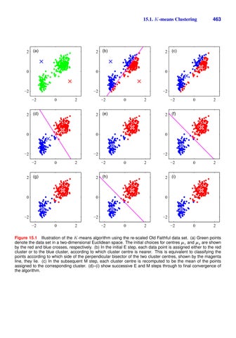
Figure 15.1 Illustration of the K-means algorithm using the re-scaled Old Faithful data set. (a) Green points denote the data set in a two-dimensional Euclidean space. The initial choices for centres µ1 and µ2 are shown by the red and blue crosses, respectively. (b) In the initial E step, each data point is assigned either to the red cluster or to the blue cluster, according to which cluster centre is nearer. This is equivalent to classifying the points according to which side of the perpendicular bisector of the two cluster centres, shown by the magenta line, they lie. (c) In the subsequent M step, each cluster centre is recomputed to be the mean of the points assigned to the corresponding cluster. (d)–(i) show successive E and M steps through to final convergence of the algorithm.