4.1. Linear Regression
Chapter 1
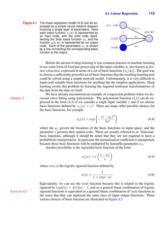
The linear regression model (4.3) can be expressed as a simple neural network diagram involving a single layer of parameters. Here each basis function φj (x) is represented by an input node, with the solid node representing the ‘bias’ basis function φ0 , and the function y(x, w) is represented by an output node. Each of the parameters wj is shown by a line connecting the corresponding basis function to the output.
φM −1 (x)
...
Figure 4.1
φ1 (x) φ0 (x)
wM −1
113
y(x, w)
w1 w0
Before the advent of deep learning it was common practice in machine learning to use some form of fixed pre-processing of the input variables x, also known as feature extraction, expressed in terms of a set of basis functions {φj (x)}. The goal was to choose a sufficiently powerful set of basis functions that the resulting learning task could be solved using a simple network model. Unfortunately, it is very difficult to hand-craft suitable basis functions for anything but the simplest applications. Deep learning avoids this problem by learning the required nonlinear transformations of the data from the data set itself. We have already encountered an example of a regression problem when we discussed curve fitting using polynomials. The polynomial function (1.1) can be expressed in the form (4.3) if we consider a single input variable x and if we choose basis functions defined by φj (x) = xj . There are many other possible choices for the basis functions, for example (x − µj )2 φj (x) = exp − (4.4) 2s2 where the µj govern the locations of the basis functions in input space, and the parameter s governs their spatial scale. These are usually referred to as ‘Gaussian’ basis functions, although it should be noted that they are not required to have a probabilistic interpretation. In particular the normalization coefficient is unimportant because these basis functions will be multiplied by learnable parameters wj . Another possibility is the sigmoidal basis function of the form x − µj (4.5) φj (x) = σ s where σ(a) is the logistic sigmoid function defined by σ(a) =
Exercise 4.3
1 . 1 + exp(−a)
(4.6)
Equivalently, we can use the tanh function because this is related to the logistic sigmoid by tanh(a) = 2σ(2a) − 1, and so a general linear combination of logistic sigmoid functions is equivalent to a general linear combination of tanh functions in the sense that they can represent the same class of input–output functions. These various choices of basis function are illustrated in Figure 4.2.