https://ebookmass.com/product/fundamentals-of-engineering-
Instant digital products (PDF, ePub, MOBI) ready for you
Download now and discover formats that fit your needs...
Thermodynamics: An Engineering Approach 9th Edition Yunus A. Çengel
https://ebookmass.com/product/thermodynamics-an-engineeringapproach-9th-edition-yunus-a-cengel/
ebookmass.com
Fundamentals of Thermodynamics 10th Edition Claus Borgnakke
https://ebookmass.com/product/fundamentals-of-thermodynamics-10thedition-claus-borgnakke/
ebookmass.com
Engineering Thermodynamics P.K. Nag
https://ebookmass.com/product/engineering-thermodynamics-p-k-nag/
ebookmass.com
It Cannoli Be Murder Catherine Bruns [Bruns
https://ebookmass.com/product/it-cannoli-be-murder-catherine-brunsbruns/
ebookmass.com
(eBook PDF) Microeconomics as a Second Language
https://ebookmass.com/product/ebook-pdf-microeconomics-as-a-secondlanguage/
ebookmass.com
Blood of the Devil W. Michael Farmer
https://ebookmass.com/product/blood-of-the-devil-w-michael-farmer/
ebookmass.com
Bears Behaving Badly Maryjanice Davidson
https://ebookmass.com/product/bears-behaving-badly-maryjanicedavidson/
ebookmass.com
The Handbook of Global Shadow Banking, Volume I: From Policy to Regulation 1st ed. Edition Luc Nijs
https://ebookmass.com/product/the-handbook-of-global-shadow-bankingvolume-i-from-policy-to-regulation-1st-ed-edition-luc-nijs/
ebookmass.com
The Complete Family Office Handbook 2nd Edition Kirby Rosplock
https://ebookmass.com/product/the-complete-family-office-handbook-2ndedition-kirby-rosplock/
ebookmass.com
Elementary Particle Physics -The Standard Theory J. Iliopoulos And T.N. Tomaras
https://ebookmass.com/product/elementary-particle-physics-thestandard-theory-j-iliopoulos-and-t-n-tomaras/
ebookmass.com
1 Getting Started 1
1.1 Using Thermodynamics 2
1.2 Defining Systems 2
1.2.1 Closed Systems 4
1.2.2 Control Volumes 4
1.2.3 Selecting the System Boundary 5
1.3 Describing Systems and Their Behavior 6
1.3.1 Macroscopic and Microscopic Views of Thermodynamics 6
1.3.2 Property, State, and Process 7
1.3.3 Extensive and Intensive Properties 7
1.3.4 Equilibrium 8
1.4 Measuring Mass, Length, Time, and Force 8
1.4.1 SI Units 9
1.4.2 English Engineering Units 10
1.5 Specific Volume 11
1.6 Pressure 12
1.6.1 Pressure Measurement 12
1.6.2 Buoyancy 14
1.6.3 Pressure Units 14
1.7 Temperature 15
1.7.1 Thermometers 16
1.7.2 Kelvin and Rankine Temperature Scales 17
1.7.3 Celsius and Fahrenheit Scales 17
1.8 Engineering Design and Analysis 19
1.8.1 Design 19
1.8.2 Analysis 19
1.9 Methodology for Solving Thermodynamics Problems 20 Chapter Summary and Study Guide 22
2 Energy
and the First Law of Thermodynamics 23
2.1 Reviewing Mechanical Concepts of Energy 24
2.1.1 Work and Kinetic Energy 24
2.1.2 Potential Energy 25
2.1.3 Units for Energy 26
2.1.4 Conservation of Energy in Mechanics 27
2.1.5 Closing Comment 27
2.2 Broadening Our Understanding of Work 27
2.2.1 Sign Convention and Notation 28
2.2.2 Power 29
2.2.3 Modeling Expansion or Compression Work 30
2.2.4 Expansion or Compression Work in Actual Processes 31
2.2.5 Expansion or Compression Work in Quasiequilibrium Processes 31
2.2.6 Further Examples of Work 34
2.2.7 Further Examples of Work in Quasiequilibrium Processes 35
2.2.8 Generalized Forces and Displacements 36
2.3 Broadening Our Understanding of Energy 36
2.4 Energy Transfer by Heat 37
2.4.1 Sign Convention, Notation, and Heat Transfer Rate 38
2.4.2 Heat Transfer Modes 39
2.4.3 Closing Comments 40
2.5 Energy Accounting: Energy Balance for Closed Systems 41
2.5.1 Important Aspects of the Energy Balance 43
2.5.2 Using the Energy Balance: Processes of Closed Systems 44
2.5.3 Using the Energy Rate Balance: Steady-State Operation 47
2.5.4 Using the Energy Rate Balance: Transient Operation 49
2.6 Energy Analysis of Cycles 50
2.6.1 Cycle Energy Balance 51
2.6.2 Power Cycles 52
2.6.3 Refrigeration and Heat Pump Cycles 52
2.7 Energy Storage 53
2.7.1 Overview 54
2.7.2 Storage Technologies 54 Chapter Summary and Study Guide 55
3 Evaluating Properties
3.1 Getting Started 58
3.1.1 Phase and Pure Substance 58
3.1.2 Fixing the State 58
3.2 p–υ–T Relation 59
3.2.1 p–υ–T Surface 60
57
3.2.2 Projections of the p–υ–T Surface 61
3.3 Studying Phase Change 63
3.4 Retrieving Thermodynamic Properties 65
3.5 Evaluating Pressure, Specific Volume, and Temperature 66
3.5.1 Vapor and Liquid Tables 66
3.5.2 Saturation Tables 68
3.6 Evaluating Specific Internal Energy and Enthalpy 72
3.6.1 Introducing Enthalpy 72
3.6.2 Retrieving u and h Data 72
3.6.3 Reference States and Reference Values 74
3.7 Evaluating Properties Using Computer Software 74
3.8 Applying the Energy Balance Using Property Tables and Software 76
3.8.1 Using Property Tables 77
3.8.2 Using Software 79
3.9
Introducing Specific Heats cυυ and cp 80
3.10 Evaluating Properties of Liquids and Solids 82
3.10.1 Approximations for Liquids Using Saturated Liquid Data 82
3.10.2 Incompressible Substance Model 83
3.11 Generalized Compressibility Chart 85
3.11.1 Universal Gas Constant, R –85
3.11.2 Compressibility Factor, Z 85
3.11.3 Generalized Compressibility Data, Z Chart 86
3.11.4 Equations of State 89
3.12 Introducing the Ideal Gas Model 90
3.12.1 Ideal Gas Equation of State 90
3.12.2 Ideal Gas Model 90
3.12.3 Microscopic Interpretation 92
3.13 Internal Energy, Enthalpy, and Specific Heats of Ideal Gases 92
3.13.1 ∆u, ∆h, cυ, and cp Relations 92
3.13.2 Using Specific Heat Functions 93
3.14 Applying the Energy Balance Using Ideal Gas Tables, Constant Specific Heats, and Software 95
3.14.1 Using Ideal Gas Tables 95
3.14.2 Using Constant Specific Heats 97
3.14.3 Using Computer Software 98
3.15 Polytropic Process Relations 100 Chapter Summary and Study Guide 102
4 Control Volume Analysis Using Energy
105
4.1 Conservation of Mass for a Control Volume 106
4.1.1 Developing the Mass Rate Balance 106
4.1.2 Evaluating the Mass Flow Rate 107
4.2 Forms of the Mass Rate Balance 107
4.2.1 One-Dimensional Flow Form of the Mass Rate Balance 108
4.2.2 Steady-State Form of the Mass Rate Balance 109
4.2.3 Integral Form of the Mass Rate Balance 109
4.3 Applications of the Mass Rate Balance 109
4.3.1 Steady-State Application 109
4.3.2 Time-Dependent (Transient) Application 110
4.4 Conservation of Energy for a Control Volume 112
4.4.1 Developing the Energy Rate Balance for a Control Volume 112
4.4.2 Evaluating Work for a Control Volume 113
4.4.3 One-Dimensional Flow Form of the Control Volume Energy Rate Balance 114
4.4.4 Integral Form of the Control Volume Energy Rate Balance 114
4.5 Analyzing Control Volumes at Steady State 115
4.5.1 Steady-State Forms of the Mass and Energy Rate Balances 115
4.5.2 Modeling Considerations for Control Volumes at Steady State 116
4.6 Nozzles and Diffusers 117
4.6.1 Nozzle and Diffuser Modeling Considerations 118
4.6.2 Application to a Steam Nozzle 118
4.7 Turbines 119
4.7.1 Steam and Gas Turbine Modeling Considerations 120
4.7.2 Application to a Steam Turbine 121
4.8 Compressors and Pumps 122
4.8.1 Compressor and Pump Modeling Considerations 122
4.8.2 Applications to an Air Compressor and a Pump System 122
4.8.3 Pumped-Hydro and Compressed-Air Energy Storage 125
4.9 Heat Exchangers 126
4.9.1 Heat Exchanger Modeling Considerations 127
4.9.2 Applications to a Power Plant Condenser and Computer Cooling 128
4.10 Throttling Devices 130
4.10.1 Throttling Device Modeling Considerations 130
4.10.2 Using a Throttling Calorimeter to Determine Quality 131
4.11 System Integration 132
4.12 Transient Analysis 135
4.12.1 The Mass Balance in Transient Analysis 135
4.12.2 The Energy Balance in Transient Analysis 135
4.12.3 Transient Analysis Applications 136 Chapter Summary and Study Guide 142
5 The Second Law of Thermodynamics
145
5.1 Introducing the Second Law 146
5.1.1 Motivating the Second Law 146
5.1.2 Opportunities for Developing Work 147
5.1.3 Aspects of the Second Law 148
5.2 Statements of the Second Law 149
5.2.1 Clausius Statement of the Second Law 149
5.2.2 Kelvin–Planck Statement of the Second Law 149
5.2.3 Entropy Statement of the Second Law 151
5.2.4 Second Law Summary 151
5.3 Irreversible and Reversible Processes 151
5.3.1 Irreversible Processes 152
5.3.2 Demonstrating Irreversibility 153
5.3.3 Reversible Processes 155
5.3.4 Internally Reversible Processes 156
5.4 Interpreting the Kelvin–Planck Statement 157
5.5 Applying the Second Law to Thermodynamic Cycles 158
5.6 Second Law Aspects of Power Cycles Interacting with Two Reservoirs 159
5.6.1 Limit on Thermal Efficiency 159
5.6.2 Corollaries of the Second Law for Power Cycles 160
5.7 Second Law Aspects of Refrigeration and Heat Pump Cycles Interacting with Two Reservoirs 161
5.7.1 Limits on Coefficients of Performance 161
5.7.2 Corollaries of the Second Law for Refrigeration and Heat Pump Cycles 162
5.8 The Kelvin and International Temperature Scales 163
5.8.1 The Kelvin Scale 163
5.8.2 The Gas Thermometer 164
5.8.3 International Temperature Scale 165
5.9 Maximum Performance Measures for Cycles Operating Between Two Reservoirs 166
5.9.1 Power Cycles 167
5.9.2 Refrigeration and Heat Pump Cycles 168
5.10 Carnot Cycle 171
5.10.1 Carnot Power Cycle 171
5.10.2 Carnot Refrigeration and Heat Pump Cycles 172
5.10.3 Carnot Cycle Summary 173
5.11 Clausius Inequality 173 Chapter Summary and Study Guide 175
6
Using Entropy 177
6.1 Entropy–A System Property 178
6.1.1 Defining Entropy Change 178
6.1.2 Evaluating Entropy 179
6.1.3 Entropy and Probability 179
6.2 Retrieving Entropy Data 179
6.2.1 Vapor Data 180
6.2.2 Saturation Data 180
6.2.3 Liquid Data 180
6.2.4 Computer Retrieval 181
6.2.5 Using Graphical Entropy Data 181
6.3 Introducing the T dS Equations 182
6.4 Entropy Change of an Incompressible Substance 184
6.5 Entropy Change of an Ideal Gas 184
6.5.1 Using Ideal Gas Tables 185
6.5.2 Assuming Constant Specific Heats 186
6.5.3 Computer Retrieval 187
6.6 Entropy Change in Internally Reversible Processes of Closed Systems 187
6.6.1 Area Representation of Heat Transfer 188
6.6.2 Carnot Cycle Application 188
6.6.3 Work and Heat Transfer in an Internally Reversible Process of Water 189
6.7 Entropy Balance for Closed Systems 190
6.7.1 Interpreting the Closed System Entropy Balance 191
6.7.2 Evaluating Entropy Production and Transfer 192
6.7.3 Applications of the Closed System Entropy Balance 192
6.7.4 Closed System Entropy Rate Balance 195
6.8 Directionality of Processes 196
6.8.1 Increase of Entropy Principle 196
6.8.2 Statistical Interpretation of Entropy 198
6.9 Entropy Rate Balance for Control Volumes 200
6.10 Rate Balances for Control Volumes at Steady State 201
6.10.1 One-Inlet, One-Exit Control Volumes at Steady State 202
6.10.2 Applications of the Rate Balances to Control Volumes at Steady State 202
6.11 Isentropic Processes 207
6.11.1 General Considerations 207
6.11.2 Using the Ideal Gas Model 208
6.11.3 Illustrations: Isentropic Processes of Air 210
6.12 Isentropic Efficiencies of Turbines, Nozzles, Compressors, and Pumps 212
6.12.1 Isentropic Turbine Efficiency 212
6.12.2 Isentropic Nozzle Efficiency 215
6.12.3 Isentropic Compressor and Pump Efficiencies 216
6.13 Heat Transfer and Work in Internally Reversible, Steady-State Flow Processes 218
6.13.1 Heat Transfer 218
6.13.2 Work 219
6.13.3 Work in Polytropic Processes 220
Chapter Summary and Study Guide 222
7 Exergy Analysis 225
7.1 Introducing Exergy 226
7.2 Conceptualizing Exergy 227
7.2.1 Environment and Dead State 227
7.2.2 Defining Exergy 228
7.3 Exergy of a System 228
7.3.1 Exergy Aspects 230
7.3.2 Specific Exergy 230
7.3.3 Exergy Change 232
7.4 Closed System Exergy Balance 233
7.4.1 Introducing the Closed System Exergy Balance 233
7.4.2 Closed System Exergy Rate Balance 236
7.4.3 Exergy Destruction and Loss 237
7.4.4 Exergy Accounting 239
7.5 Exergy Rate Balance for Control Volumes at Steady State 240
7.5.1 Comparing Energy and Exergy for Control Volumes at Steady State 242
7.5.2 Evaluating Exergy Destruction in Control Volumes at Steady State 243
7.5.3 Exergy Accounting in Control Volumes at Steady State 246
7.6 Exergetic (Second Law) Efficiency 249
7.6.1 Matching End Use to Source 249
7.6.2 Exergetic Efficiencies of Common Components 251
7.6.3 Using Exergetic Efficiencies 253
7.7 Thermoeconomics 253
7.7.1 Costing 254
7.7.2 Using Exergy in Design 254
7.7.3 Exergy Costing of a Cogeneration System 256 Chapter Summary and Study Guide 260
8 Vapor Power Systems 261
8.1 Introducing Vapor Power Plants 266
8.2 The Rankine Cycle 268
8.2.1 Modeling the Rankine Cycle 269
8.2.2 Ideal Rankine Cycle 271
8.2.3 Effects of Boiler and Condenser Pressures on the Rankine Cycle 274
8.2.4 Principal Irreversibilities and Losses 276
8.3 Improving Performance—Superheat, Reheat, and Supercritical 279
8.4 Improving Performance—Regenerative Vapor Power Cycle 284
8.4.1 Open Feedwater Heaters 284
8.4.2 Closed Feedwater Heaters 287
8.4.3 Multiple Feedwater Heaters 289
8.5 Other Vapor Power Cycle Aspects 292
8.5.1 Working Fluids 292
8.5.2 Cogeneration 293
8.5.3 Carbon Capture and Storage 295
8.6 Case Study: Exergy Accounting of a Vapor Power Plant 296
Chapter Summary and Study Guide 301
9 Gas Power Systems 303
9.1 Introducing Engine Terminology 304
9.2 Air-Standard Otto Cycle 306
9.3 Air-Standard Diesel Cycle 311
9.4 Air-Standard Dual Cycle 314
9.5 Modeling Gas Turbine Power Plants 317
9.6 Air-Standard Brayton Cycle 318
9.6.1 Evaluating Principal Work and Heat Transfers 318
9.6.2 Ideal Air-Standard Brayton Cycle 319
9.6.3 Considering Gas Turbine Irreversibilities and Losses 324
9.7 Regenerative Gas Turbines 326
9.8 Regenerative Gas Turbines with Reheat and Intercooling 329
9.8.1 Gas Turbines with Reheat 329
9.8.2 Compression with Intercooling 331
9.8.3 Reheat and Intercooling 335
9.8.4 Ericsson and Stirling Cycles 337
9.9 Gas Turbine–Based Combined Cycles 339
9.9.1 Combined Gas Turbine–Vapor Power Cycle 339
9.9.2 Cogeneration 344
9.10 Integrated Gasification Combined-Cycle Power Plants 344
9.11 Gas Turbines for Aircraft Propulsion 346
9.12 Compressible Flow Preliminaries 350
9.12.1 Momentum Equation for Steady One-Dimensional Flow 350
9.12.2 Velocity of Sound and Mach Number 351
9.12.3 Determining Stagnation State Properties 353
9.13 Analyzing One-Dimensional Steady Flow in Nozzles and Diffusers 353
9.13.1 Exploring the Effects of Area Change in Subsonic and Supersonic Flows 353
9.13.2 Effects of Back Pressure on Mass Flow Rate 356
9.13.3 Flow Across a Normal Shock 358
9.14 Flow in Nozzles and Diffusers of Ideal Gases with Constant Specific Heats 359
9.14.1 Isentropic Flow Functions 359
9.14.2 Normal Shock Functions 362
Chapter Summary and Study Guide 366
10 Refrigeration and Heat Pump Systems
369
10.1 Vapor Refrigeration Systems 370
10.1.1 Carnot Refrigeration Cycle 370
10.1.2 Departures from the Carnot Cycle 371
10.2 Analyzing Vapor-Compression Refrigeration Systems 372
10.2.1 Evaluating Principal Work and Heat Transfers 372
10.2.2 Performance of Ideal Vapor-Compression Systems 373
10.2.3 Performance of Actual Vapor-Compression Systems 375
10.2.4 The p–h Diagram 378
10.3 Selecting Refrigerants 379
10.4 Other Vapor-Compression Applications 382
10.4.1 Cold Storage 382
10.4.2 Cascade Cycles 383
10.4.3 Multistage Compression with Intercooling 384
10.5 Absorption Refrigeration 385
10.6 Heat Pump Systems 386
10.6.1 Carnot Heat Pump Cycle 387
10.6.2 Vapor-Compression Heat Pumps 387
10.7 Gas Refrigeration Systems 390
10.7.1 Brayton Refrigeration Cycle 390
10.7.2 Additional Gas Refrigeration Applications 394
10.7.3 Automotive Air Conditioning Using Carbon Dioxide 395
Chapter Summary and Study Guide 396
11 Thermodynamic Relations 399
11.1 Using Equations of State 400
11.1.1 Getting Started 400
11.1.2 Two-Constant Equations of State 401
11.1.3 Multiconstant Equations of State 404
11.2 Important Mathematical Relations 405
11.3 Developing Property Relations 408
11.3.1 Principal Exact Differentials 408
11.3.2 Property Relations from Exact Differentials 409
11.3.3 Fundamental Thermodynamic Functions 413
11.4 Evaluating Changes in Entropy, Internal Energy, and Enthalpy 414
11.4.1 Considering Phase Change 414
11.4.2 Considering Single-Phase Regions 417
11.5 Other Thermodynamic Relations 422
11.5.1 Volume Expansivity, Isothermal and Isentropic Compressibility 422
11.5.2 Relations Involving Specific Heats 423
11.5.3 Joule–Thomson Coefficient 426
11.6 Constructing Tables of Thermodynamic Properties 428
11.6.1 Developing Tables by Integration Using p–υ–T and Specific Heat Data 428
11.6.2 Developing Tables by Differentiating a Fundamental Thermodynamic Function 430
11.7 Generalized Charts for Enthalpy and Entropy 432
11.8 p–υ–T Relations for Gas Mixtures 438
11.9 Analyzing Multicomponent Systems 442
11.9.1 Partial Molal Properties 443
11.9.2 Chemical Potential 445
11.9.3 Fundamental Thermodynamic Functions for Multicomponent Systems 446
11.9.4 Fugacity 448
11.9.5 Ideal Solution 451
11.9.6 Chemical Potential for Ideal Solutions 452 Chapter Summary and Study Guide 453
12 Ideal Gas Mixture and Psychrometric Applications
12.1 Describing Mixture Composition 458
457
12.2 Relating p, V, and T for Ideal Gas Mixtures 461
12.3 Evaluating U, H, S, and Specific Heats 463
12.3.1 Evaluating U and H 463
12.3.2 Evaluating cυ and cp 463
12.3.3 Evaluating S 464
12.3.4 Working on a Mass Basis 464
12.4 Analyzing Systems Involving Mixtures 465
12.4.1 Mixture Processes at Constant Composition 465
12.4.2 Mixing of Ideal Gases 470
12.5 Introducing Psychrometric Principles 474
12.5.1 Moist Air 474
12.5.2 Humidity Ratio, Relative Humidity, Mixture Enthalpy, and Mixture Entropy 475
12.5.3 Modeling Moist Air in Equilibrium with Liquid Water 477
12.5.4 Evaluating the Dew Point Temperature 478
12.5.5 Evaluating Humidity Ratio Using the Adiabatic-Saturation Temperature 482
12.6 Psychrometers: Measuring the Wet-Bulb and Dry-Bulb Temperatures 483
12.7 Psychrometric Charts 484
12.8 Analyzing Air-Conditioning Processes 486
12.8.1 Applying Mass and Energy Balances to Air-Conditioning Systems 486
12.8.2 Conditioning Moist Air at Constant Composition 488
12.8.3 Dehumidification 490
12.8.4 Humidification 493
12.8.5 Evaporative Cooling 494
12.8.6 Adiabatic Mixing of Two Moist Air Streams 496
12.9 Cooling Towers 499
Chapter Summary and Study Guide 501
13 Reacting Mixtures and Combustion
503
13.1 Introducing Combustion 504
13.1.1 Fuels 505
13.1.2 Modeling Combustion Air 505
13.1.3 Determining Products of Combustion 508
13.1.4 Energy and Entropy Balances for Reacting Systems 511
13.2 Conservation of Energy—Reacting Systems 511
13.2.1 Evaluating Enthalpy for Reacting Systems 511
13.2.2 Energy Balances for Reacting Systems 514
13.2.3 Enthalpy of Combustion and Heating Values 520
13.3 Determining the Adiabatic Flame Temperature 523
13.3.1 Using Table Data 523
13.3.2 Using Computer Software 523
13.3.3 Closing Comments 525
13.4 Fuel Cells 526
13.4.1 Proton Exchange Membrane Fuel Cell 527
13.4.2 Solid Oxide Fuel Cell 529
13.5 Absolute Entropy and the Third Law of Thermodynamics 530
13.5.1 Evaluating Entropy for Reacting Systems 530
13.5.2 Entropy Balances for Reacting Systems 531
13.5.3 Evaluating Gibbs Function for Reacting Systems 534
13.6 Conceptualizing Chemical Exergy 536
13.6.1 Working Equations for Chemical Exergy 538
13.6.2 Evaluating Chemical Exergy for Several Cases 538
13.6.3 Closing Comments 540
13.7 Standard Chemical Exergy 540
13.7.1 Standard Chemical Exergy of a Hydrocarbon: CaHb 541
13.7.2 Standard Chemical Exergy of Other Substances 544
13.8 Applying Total Exergy 545
13.8.1 Calculating Total Exergy 545
13.8.2 Calculating Exergetic Efficiencies of Reacting Systems 549
Chapter Summary and Study Guide 552
14 Chemical and Phase Equilibrium 555
14.1 introducing Equilibrium Criteria 556
14.1.1 Chemical Potential and Equilibrium 557
14.1.2 Evaluating Chemical Potentials 559
14.2 Equation of Reaction Equilibrium 560
14.2.1 Introductory Case 560
14.2.2 General Case 561
14.3 Calculating Equilibrium Compositions 562
14.3.1 Equilibrium Constant for Ideal Gas Mixtures 562
14.3.2 Illustrations of the Calculation of Equilibrium Compositions for Reacting Ideal Gas Mixtures 565
14.3.3 Equilibrium Constant for Mixtures and Solutions 569
14.4 Further Examples of the Use of the Equilibrium Constant 570
14.4.1 Determining Equilibrium Flame Temperature 570
14.4.2 Van’t Hoff Equation 573
14.4.3 Ionization 574
14.4.4 Simultaneous Reactions 575
14.5 Equilibrium between Two Phases of a Pure Substance 578
14.6 Equilibrium of Multicomponent, Multiphase Systems 579
14.6.1 Chemical Potential and Phase Equilibrium 580
14.6.2 Gibbs Phase Rule 582
Chapter Summary and Study Guide 583
appendix Tables, Figures, and Charts
a-1
Index to Tables in SI Units a-1
Index to Tables in English Units a-49
Index to Figures and Charts a-97
Index i-1
thermodynamics
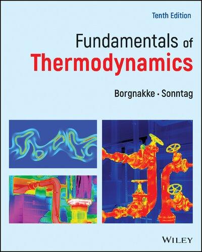
Engineers use principles drawn from thermodynamics and other engineering sciences, including fluid mechanics and heat and mass transfer, to analyze and design devices intended to meet human needs. Throughout the twentieth century, engineering applications of thermodynamics helped pave the way for significant improvements in our quality of life with advances in major areas such as surface transportation, air travel, space flight, electricity generation and transmission, building heating and cooling, and improved medical practices. The wide realm of these applications is suggested by Table 1.1.
In the twenty-first century, engineers will create the technology needed to achieve a sustainable future. Thermodynamics will continue to advance human well-being by addressing looming societal challenges owing to declining supplies of energy resources: oil, natural gas, coal, and fissionable material; effects of global climate change; and burgeoning population. Life in the United States is expected to change in several important respects by mid-century. In the area of power use, for example, electricity will play an even greater role than today. Table 1.2 provides predictions of other changes experts say will be observed.
If this vision of mid-century life is correct, it will be necessary to evolve quickly from our present energy posture. As was the case in the twentieth century, thermodynamics will contribute significantly to meeting the challenges of the twenty-first century, including using fossil fuels more effectively, advancing renewable energy technologies, and developing more energy-efficient transportation systems, buildings, and industrial practices. Thermodynamics also will play a role in mitigating global climate change, air pollution, and water pollution. Applications will be observed in bioengineering, biomedical systems, and the deployment of nanotechnology. This book provides the tools needed by specialists working in all such fields. For nonspecialists, the book provides background for making decisions about technology related to thermodynamics—on the job, as informed citizens, and as government leaders and policy makers.
1.2
Defining Systems
The key initial step in any engineering analysis is to describe precisely what is being studied. In mechanics, if the motion of a body is to be determined, normally the first step is to define a free body and identify all the forces exerted on it by other bodies. Newton’s second law of motion is then applied. In thermodynamics the term system is used to identify the subject of the analysis. Once the system is defined and the relevant interactions with other systems are identified, one or more physical laws or relations are applied.
The system is whatever we want to study. It may be as simple as a free body or as complex as an entire chemical refinery. We may want to study a quantity of matter contained within a closed, rigid-walled tank, or we may want to consider something such as a pipeline through which natural gas flows. The composition of the matter inside the system may be fixed or may be changing through chemical or nuclear reactions. The shape or volume of the system being analyzed is not necessarily constant, as when a gas in a cylinder is compressed by a piston or a balloon is inflated.
surroundings boundary
Everything external to the system is considered to be part of the system’s surroundings The system is distinguished from its surroundings by a specified boundary, which may be at rest or in motion. You will see that the interactions between a system and its surroundings, which take place across the boundary, play an important part in engineering thermodynamics.
Two basic kinds of systems are distinguished in this book. These are referred to, respectively, as closed systems and control volumes. A closed system refers to a fixed quantity of matter, whereas a control volume is a region of space through which mass may flow. The term control mass is sometimes used in place of closed system, and the term open system is used interchangeably with control volume. When the terms control mass and control volume are used, the system boundary is often referred to as a control surface
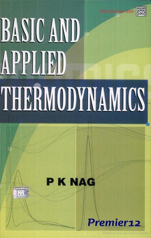
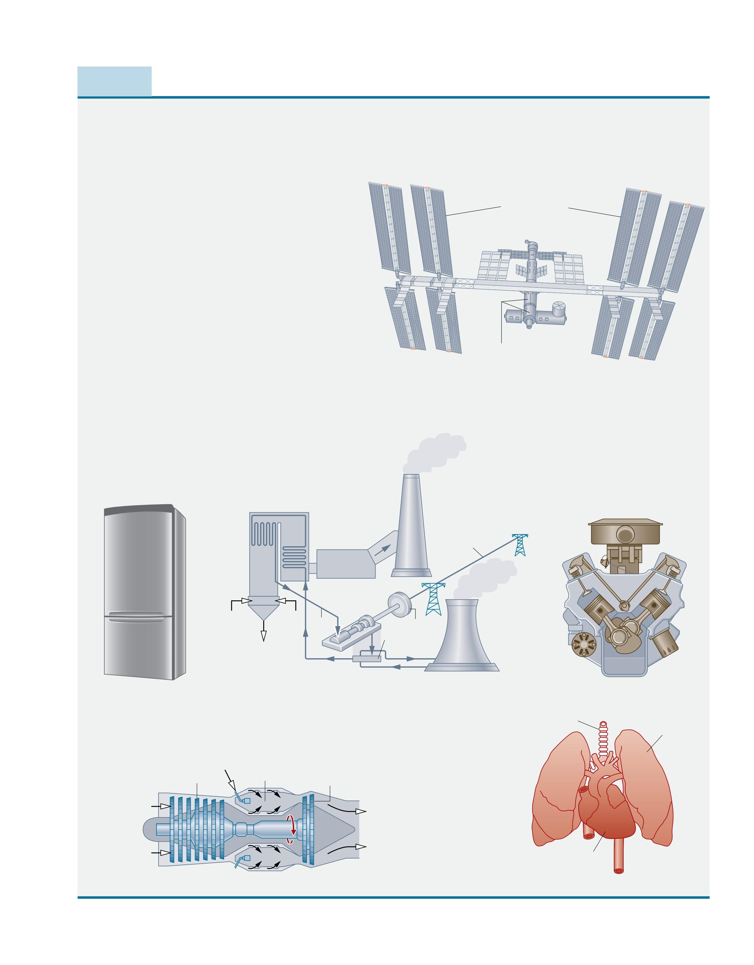
t ABLE 1.1 selected Areas of Application of Engineering thermodynamics
Aircraft and rocket propulsion
Alternative energy systems
Fuel cells
Geothermal systems
Magnetohydrodynamic (MhD) converters
Ocean thermal, wave, and tidal power generation
Solar-activated heating, cooling, and power generation
thermoelectric and thermionic devices
Wind turbines
Automobile engines
Bioengineering applications
Biomedical applications
Combustion systems
Compressors, pumps
Cooling of electronic equipment
Cryogenic systems, gas separation, and liquefaction
Fossil and nuclear-fueled power stations
heating, ventilating, and air-conditioning systems
Absorption refrigeration and heat pumps
Vapor-compression refrigeration and heat pumps
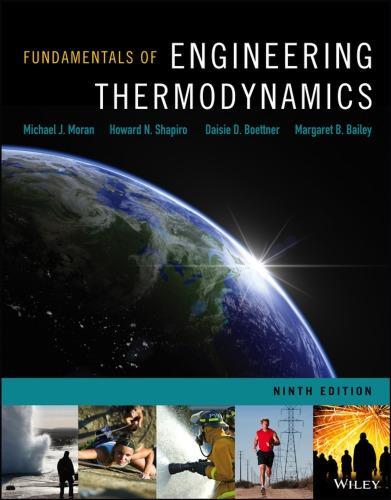
Steam and gas turbines power production propulsion
Space Station
Space Station
t ABLE 1.2 Predictions of Life in the united states in 2050
At home
• homes are constructed better to reduce heating and cooling needs.
• homes have systems for electronically monitoring and regulating energy use.
• Appliances and heating and air-conditioning systems are more energy-efficient.
• Use of solar energy for space and water heating is common.
• More food is produced locally.
transportation
• plug-in hybrid vehicles and all-electric vehicles dominate.
• One-quarter of transport fuel is biofuels.
• Use of public transportation within and between cities is common.
• An expanded passenger railway system is widely used.
Lifestyle
• Efficient energy-use practices are utilized throughout society.
• Recycling is widely practiced, including recycling of water.
• Distance learning is common at most educational levels.
• telecommuting and teleconferencing are the norm.
• the Internet is predominately used for consumer and business commerce.
Power generation
• Electricity plays a greater role throughout society.
• Wind, solar, and other renewable technologies contribute a significant share of the nation’s electricity needs.
• A mix of conventional fossil-fueled and nuclear power plants provides a smaller, but still significant, share of the nation’s electricity needs.
• A smart and secure national power transmission grid is in place.
1.2.1 Closed Systems
A closed system is defined when a particular quantity of matter is under study. A closed system always contains the same matter. There can be no transfer of mass across its boundary. A special type of closed system that does not interact in any way with its surroundings is called an isolated system
Figure 1.1 shows a gas in a piston–cylinder assembly. When the valves are closed, we can consider the gas to be a closed system. The boundary lies just inside the piston and cylinder walls, as shown by the dashed lines on the figure. Since the portion of the boundary between the gas and the piston moves with the piston, the system volume varies. No mass would cross this or any other part of the boundary. If combustion occurs, the composition of the system changes as the initial combustible mixture becomes products of combustion.
1.2.2 Control Volumes
In subsequent sections of this book, we perform thermodynamic analyses of devices such as turbines and pumps through which mass flows. These analyses can be conducted in principle by studying a particular quantity of matter, a closed system, as it passes through the device. In most cases it is simpler to think instead in terms of a given region of space through which mass flows. With this approach, a region within a prescribed boundary is studied. The region is called a control volume. Mass crosses the boundary of a control volume.
A diagram of an engine is shown in Fig. 1.2a. The dashed line defines a control volume that surrounds the engine. Observe that air, fuel, and exhaust gases cross the boundary. A schematic such as in Fig. 1.2b often suffices for engineering analysis. Control volume applications in biology and botany are illustrated is Figs. 1.3 and 1.4 respectively.
Boundary Gas
F
I g. 1.1 Closed system: A gas in a piston–cylinder assembly.
(control surface) Boundary (control surface)
1.2.3 Selecting the System Boundary
The system boundary should be delineated carefully before proceeding with any thermodynamic analysis. However, the same physical phenomena often can be analyzed in terms of alternative choices of the system, boundary, and surroundings. The choice of a particular boundary defining a particular system depends heavily on the convenience it allows in the subsequent analysis.
In general, the choice of system boundary is governed by two considerations: (1) what is known about a possible system, particularly at its boundaries, and (2) the objective of the analysis.
For Exampl E
Figure 1.5 shows a sketch of an air compressor connected to a storage tank. The system boundary shown on the figure encloses the compressor, tank, and all of the piping. This boundary might be selected if the electrical power input is known, and the objective of the analysis is to determine how long the compressor must operate for the pressure in the tank to rise to a specified value. Since mass crosses the boundary, the system would be a control volume. a control volume enclosing only the compressor might be chosen if the condition of the air entering and exiting the compressor is known, and the objective is to determine the electric power input.
drink)
Driveshaft
Driveshaft
System Types Tabs a, b, and c
Ta KE N o TE...
animations reinforce many of the text presentations. You can view these animations by going to the e-book, WileyplUS course, or student companion site for this book. animations are keyed to specific content by an adjacent icon.
The first of these icons appears here. In this example, the animation name “System Types” refers to the animation content while “Tabs a, b, and c” refers to the tabs of the animation recommended for viewing now to enhance your understanding.
1.3
Describing Systems and their Behavior
Engineers are interested in studying systems and how they interact with their surroundings. In this section, we introduce several terms and concepts used to describe systems and how they behave.
1.3.1 Macroscopic and Microscopic Views of thermodynamics
Systems can be studied from a macroscopic or a microscopic point of view. The macroscopic approach to thermodynamics is concerned with the gross or overall behavior. This is sometimes called classical thermodynamics. No model of the structure of matter at the molecular, atomic, and subatomic levels is directly used in classical thermodynamics. Although the behavior of systems is affected by molecular structure, classical thermodynamics allows important aspects of system behavior to be evaluated from observations of the overall system.
The microscopic approach to thermodynamics, known as statistical thermodynamics, is concerned directly with the structure of matter. The objective of statistical thermodynamics is to characterize by statistical means the average behavior of the particles making up a system of interest and relate this information to the observed macroscopic behavior of the system. For applications involving lasers, plasmas, high-speed gas flows, chemical kinetics, very low temperatures (cryogenics), and others, the methods of statistical thermodynamics are essential. The microscopic approach is used in this text to interpret internal energy in Chap. 2 and entropy in Chap 6. Moreover, as noted in Chap. 3, the microscopic approach is instrumental in developing certain data, for example ideal gas specific heats. For a wide range of engineering applications, classical thermodynamics not only provides a considerably more direct approach for analysis and design but also requires far fewer mathematical complications. For these reasons the macroscopic viewpoint is the one adopted in this book. Finally, relativity effects are not significant for the systems under consideration in this book.
Animation
F I g. 1.5 Air compressor and storage tank.
1.3.2 property, State, and process
To describe a system and predict its behavior requires knowledge of its properties and how those properties are related. A property is a macroscopic characteristic of a system such as mass, volume, energy, pressure, and temperature to which a numerical value can be assigned at a given time without knowledge of the previous behavior (history) of the system.
The word state refers to the condition of a system as described by its properties. Since there are normally relations among the properties of a system, the state often can be specified by providing the values of a subset of the properties. All other properties can be determined in terms of these few.
When any of the properties of a system changes, the state changes and the system is said to undergo a process. A process is a transformation from one state to another. If a system exhibits the same values of its properties at two different times, it is in the same state at these times. A system is said to be at steady state if none of its properties changes with time.
Many properties are considered during the course of our study of engineering thermodynamics. Thermodynamics also deals with quantities that are not properties, such as mass flow rates and energy transfers by work and heat. Additional examples of quantities that are not properties are provided in subsequent chapters. For a way to distinguish properties from nonproperties, see the following box.
Distinguishing Properties from Nonproperties
At a given state, each property has a definite value that can be assigned without knowledge of how the system arrived at that state. The change in value of a property as the system is altered from one state to another is determined, therefore, solely by the two end states and is independent of the particular way the change of state occurred. The change is independent of the details of the process. Conversely,
1.3.3 Extensive and Intensive properties
if the value of a quantity is independent of the process between two states, then that quantity is the change in a property. This provides a test for determining whether a quantity is a property: A quantity is a property if, and only if, its change in value between two states is independent of the process. It follows that if the value of a particular quantity depends on the details of the process, and not solely on the end states, that quantity cannot be a property.
Thermodynamic properties can be placed in two general classes: extensive and intensive. A property is called extensive if its value for an overall system is the sum of its values for the parts into which the system is divided. Mass, volume, energy, and several other properties introduced later are extensive. Extensive properties depend on the size or extent of a system. The extensive properties of a system can change with time, and many thermodynamic analyses consist mainly of carefully accounting for changes in extensive properties such as mass and energy as a system interacts with its surroundings.
Intensive properties are not additive in the sense previously considered. Their values are independent of the size or extent of a system and may vary from place to place within the system at any moment. Intensive properties may be functions of both position and time, whereas extensive properties can vary only with time. Specific volume (Sec. 1.5), pressure, and temperature are important intensive properties; several other intensive properties are introduced in subsequent chapters.
For Exampl E
To illustrate the difference between extensive and intensive properties, consider an amount of matter that is uniform in temperature, and imagine that it is composed of several parts, as illustrated in Fig. 1.6. The mass of the whole is the sum of the masses of the parts, and the overall volume is the sum of the volumes of the parts. However, the temperature of the whole is not the sum of the temperatures of the parts; it is the same for each part. mass and volume are extensive, but temperature is intensive.
extensive property
intensive property
Extensive and Intensive Properties Tab a
Animation
1.3.4 Equilibrium
Classical thermodynamics places primary emphasis on equilibrium states and changes from one equilibrium state to another. Thus, the concept of equilibrium is fundamental. In mechanics, equilibrium means a condition of balance maintained by an equality of opposing forces. In thermodynamics, the concept is more far-reaching, including not only a balance of forces but also a balance of other influences. Each kind of influence refers to a particular aspect of thermodynamic, or complete, equilibrium. Accordingly, several types of equilibrium must exist individually to fulfill the condition of complete equilibrium; among these are mechanical, thermal, phase, and chemical equilibrium.
Criteria for these four types of equilibrium are considered in subsequent discussions. For the present, we may think of testing to see if a system is in thermodynamic equilibrium by the following procedure: Isolate the system from its surroundings and watch for changes in its observable properties. If there are no changes, we conclude that the system was in equilibrium at the moment it was isolated. The system can be said to be at an equilibrium state
When a system is isolated, it does not interact with its surroundings; however, its state can change as a consequence of spontaneous events occurring internally as its intensive properties, such as temperature and pressure, tend toward uniform values. When all such changes cease, the system is in equilibrium. At equilibrium, temperature is uniform throughout the system. Also, pressure can be regarded as uniform throughout as long as the effect of gravity is not significant; otherwise, a pressure variation can exist, as in a vertical column of liquid.
It is not necessary that a system undergoing a process be in equilibrium during the process. Some or all of the intervening states may be nonequilibrium states. For many such processes, we are limited to knowing the state before the process occurs and the state after the process is completed.
1.4
Measuring Mass, Length, time, and Force
When engineering calculations are performed, it is necessary to be concerned with the units of the physical quantities involved. A unit is any specified amount of a quantity by comparison with which any other quantity of the same kind is measured. For example, meters, centimeters, kilometers, feet, inches, and miles are all units of length. Seconds, minutes, and hours are alternative time units.
Because physical quantities are related by definitions and laws, a relatively small number of physical quantities suffice to conceive of and measure all others. These are called primary dimensions. The others are measured in terms of the primary dimensions and are called secondary. For example, if length and time were regarded as primary, velocity and area would be secondary. A set of primary dimensions that suffice for applications in mechanics is mass, length, and time. Additional primary dimensions are required when additional physical phenomena come under consideration. Temperature is included for thermodynamics, and electric current is introduced for applications involving electricity.
Once a set of primary dimensions is adopted, a base unit for each primary dimension is specified. Units for all other quantities are then derived in terms of the base units. Let us illustrate these ideas by considering briefly two systems of units: SI units and English Engineering units.
F I g. 1.6 Figure used to discuss the extensive and intensive property concepts.
t ABLE 1.3 units for mass, Length, time, and Force sI
1.4.1 SI Units
In the present discussion we consider the SI system of units that takes mass, length, and time as primary dimensions and regards force as secondary. SI is the abbreviation for Système International d’Unités (International System of Units), which is the legally accepted system in most countries. The conventions of the SI are published and controlled by an international treaty organization. The SI base units for mass, length, and time are listed in Table 1.3 and discussed in the following paragraphs. The SI base unit for temperature is the kelvin, K.
The SI base unit of mass is the kilogram, kg. It is equal to the mass of a particular cylinder of platinum–iridium alloy kept by the International Bureau of Weights and Measures near Paris. The mass standard for the United States is maintained by the National Institute of Standards and Technology (NIST). The kilogram is the only base unit still defined relative to a fabricated object.
The SI base unit of length is the meter (metre), m, defined as the length of the path traveled by light in a vacuum during a specified time interval. The base unit of time is the second, s. The second is defined as the duration of 9,192,631,770 cycles of the radiation associated with a specified transition of the cesium atom.
The SI unit of force, called the newton, is a secondary unit, defined in terms of the base units for mass, length, and time. Newton’s second law of motion states that the net force acting on a body is proportional to the product of the mass and the acceleration, written F ∝ ma. The newton is defined so that the proportionality constant in the expression is equal to unity. That is, Newton’s second law is expressed as the equality Fma = (1.1)
The newton, N, is the force required to accelerate a mass of 1 kilogram at the rate of 1 meter per second per second. With Eq. 1.1
1 N(1 kg)(1 m/s) 1 kg m/s 22 ⋅⋅ == (1.2)
SI base units
For Exampl E
To illustrate the use of the SI units introduced thus far, let us determine the weight in newtons of an object whose mass is 1000 kg, at a place on Earth’s surface where the acceleration due to gravity equals a standard value defined as 9.80665 m/s2. recalling that the weight of an object refers to the force of gravity and is calculated using the mass of the object, m, and the local acceleration of gravity, g, with Eq. 1.1 we get
(1000 kg)(9.80665 m/s )9806.65 kg m/s 22
This force can be expressed in terms of the newton by using Eq. 1.2 as a unit conversion factor. That is,
Ta KE N o TE...
observe that in the calculation of force in newtons, the unit conversion factor is set off by a pair of vertical lines. This device is used throughout the text to identify unit conversions.
t ABLE 1.4 sI unit Prefixes
symbol
English base units
Since weight is calculated in terms of the mass and the local acceleration due to gravity, the weight of an object can vary because of the variation of the acceleration of gravity with location, but its mass remains constant.
For Exampl E
If the object considered previously were on the surface of a planet at a point where the acceleration of gravity is one-tenth of the value used in the above calculation, the mass would remain the same but the weight would be one-tenth of the calculated value.
SI units for other physical quantities are also derived in terms of the SI base units. Some of the derived units occur so frequently that they are given special names and symbols, such as the newton. SI units for quantities pertinent to thermodynamics are given as they are introduced in the text. Since it is frequently necessary to work with extremely large or small values when using the SI unit system, a set of standard prefixes is provided in Table 1.4 to simplify matters. For example, km denotes kilometer, that is, 103 m.
1.4.2
English Engineering Units
Although SI units are the worldwide standard, at the present time many segments of the engineering community in the United States regularly use other units. A large portion of America’s stock of tools and industrial machines and much valuable engineering data utilize units other than SI units. For many years to come, engineers in the United States will have to be conversant with a variety of units.
In this section we consider a system of units that is commonly used in the United States, called the English Engineering system. The English base units for mass, length, and time are listed in Table 1.3 and discussed in the following paragraphs. English units for other quantities pertinent to thermodynamics are given as they are introduced in the text.
The base unit for length is the foot, ft, defined in terms of the meter as 1 ft 0.3048 m =
The inch, in., is defined in terms of the foot: 12 in. 1 ft =
One inch equals 2.54 cm. Although units such as the minute and the hour are often used in engineering, it is convenient to select the second as the English Engineering base unit for time.
The English Engineering base unit of mass is the pound mass, lb, defined in terms of the kilogram as
The symbol lbm also may be used to denote the pound mass.
Once base units have been specified for mass, length, and time in the English Engineering system of units, a force unit can be defined, as for the newton, using Newton’s second law written as Eq. 1.1. From this viewpoint, the English unit of force, the pound force, lbf, is the force required to accelerate one pound mass at 32.1740 ft/s2, which is the standard acceleration of gravity. Substituting values into Eq. 1.1, 1 lbf(1 lb)(32.1740 ft/s) 32.1740 lbft/s 22 ==
With this approach force is regarded as secondary.
The pound force, lbf, is not equal to the pound mass, lb, introduced previously. Force and mass are fundamentally different, as are their units. The double use of the word “pound” can be confusing, so care must be taken to avoid error.
For Exampl E
To show the use of these units in a single calculation, let us determine the weight of an object whose mass is 1000 lb at a location where the local acceleration of gravity is 32.0 ft/s2. By inserting values into Eq. 1.1 and using Eq. 1.5 as a unit conversion factor, we get
This calculation illustrates that the pound force is a unit of force distinct from the pound mass, a unit of mass.
1.5 Specific Volume
Three measurable intensive properties that are particularly important in engineering thermodynamics are specific volume, pressure, and temperature. Specific volume is considered in this section. Pressure and temperature are considered in Secs. 1.6 and 1.7, respectively.
From the macroscopic perspective, the description of matter is simplified by considering it to be distributed continuously throughout a region. The correctness of this idealization, known as the continuum hypothesis, is inferred from the fact that for an extremely large class of phenomena of engineering interest the resulting description of the behavior of matter is in agreement with measured data.
When substances can be treated as continua, it is possible to speak of their intensive thermodynamic properties “at a point.” Thus, at any instant the density ρ at a point is defined as
where V ′ is the smallest volume for which a definite value of the ratio exists. The volume V ′ contains enough particles for statistical averages to be significant. It is the smallest volume for which the matter can be considered a continuum and is normally small enough that it can be considered a “point.” With density defined by Eq. 1.6, density can be described mathematically as a continuous function of position and time.
The density, or local mass per unit volume, is an intensive property that may vary from point to point within a system. Thus, the mass associated with a particular volume V is determined in principle by integration
and not simply as the product of density and volume.
The specific volume υ is defined as the reciprocal of the density, υ = 1/ρ. It is the volume per unit mass. Like density, specific volume is an intensive property and may vary from point to point. SI units for density and specific volume are kg/m3 and m3/kg, respectively. They are also often expressed, respectively, as g/cm3 and cm3/g. English units used for density and specific volume in this text are lb/ft3 and ft3/lb, respectively. In certain applications it is convenient to express properties such as specific volume on a molar basis rather than on a mass basis. A mole is an amount of a given substance numerically equal to its molecular weight. In this book we express the amount of substance on a molar basis in terms of the kilomole (kmol) or the pound mole (lbmol), as appropriate. In each case we use
Extensive and Intensive Properties Tabs b and c
The number of kilomoles of a substance, n, is obtained by dividing the mass, m, in kilograms by the molecular weight, M, in kg/kmol. Similarly, the number of pound moles, n, is obtained by dividing the mass, m, in pound mass by the molecular weight, M, in lb/lbmol. When m is in grams, Eq. 1.8 gives n in gram moles, or mol for short. Recall from chemistry that the number of molecules in a gram mole, called Avogadro’s number, is 6.022 × 10²³. Appendix Tables A-1 and A-1E provide molecular weights for several substances.
To signal that a property is on a molar basis, a bar is used over its symbol. Thus, υ signifies the volume per kmol or lbmol, as appropriate. In this text, the units used for υ are m3/kmol and ft3/lbmol. With Eq. 1.8, the relationship between υ and υ is
where M is the molecular weight in kg/kmol or lb/lbmol, as appropriate.
1.6 pressure
Next, we introduce the concept of pressure from the continuum viewpoint. Let us begin by considering a small area, A, passing through a point in a fluid at rest. The fluid on one side of the area exerts a compressive force on it that is normal to the area, Fnormal. An equal but oppositely directed force is exerted on the area by the fluid on the other side. For a fluid at rest, no other forces than these act on the area. The pressure, p, at the specified point is defined as the limit
where A′ is the area at the “point” in the same limiting sense as used in the definition of density. If the area A′ was given new orientations by rotating it around the given point, and the pressure determined for each new orientation, it would be found that the pressure at the point is the same in all directions as long as the fluid is at rest. This is a consequence of the equilibrium of forces acting on an element of volume surrounding the point. However, the pressure can vary from point to point within a fluid at rest; examples are the variation of atmospheric pressure with elevation and the pressure variation with depth in oceans, lakes, and other bodies of water. Consider next a fluid in motion. In this case the force exerted on an area passing through a point in the fluid may be resolved into three mutually perpendicular components: one normal to the area and two in the plane of the area. When expressed on a unit area basis, the component normal to the area is called the normal stress, and the two components in the plane of the area are termed shear stresses. The magnitudes of the stresses generally vary with the orientation of the area. The state of stress in a fluid in motion is a topic that is normally treated thoroughly in fluid mechanics. The deviation of a normal stress from the pressure, the normal stress that would exist were the fluid at rest, is typically very small. In this book we assume that the normal stress at a point is equal to the pressure at that point. This assumption yields results of acceptable accuracy for the applications considered. Also, the term pressure, unless stated otherwise, refers to absolute pressure: pressure with respect to the zero pressure of a complete vacuum. The lowest possible value of absolute pressure is zero.
1.6.1
pressure Measurement
Manometers and barometers measure pressure in terms of the length of a column of liquid such as mercury, water, or oil. The manometer shown in Fig. 1.7 has one end open to the atmosphere and the other attached to a tank containing a gas at a uniform pressure. Since pressures at equal elevations in a continuous mass of a liquid or gas at rest are equal, the pressures at points a and b of Fig. 1.7 are equal. Applying an elementary force balance, the gas pressure is
where patm is the local atmospheric pressure, ρ is the density of the manometer liquid, g is the acceleration of gravity, and L is the difference in the liquid levels.
The barometer shown in Fig. 1.8 is formed by a closed tube filled with liquid mercury and a small amount of mercury vapor inverted in an open container of liquid mercury. Since the pressures at points a and b are equal, a force balance gives the atmospheric pressure as pp gL atmvapor mρ =+ (1.12)
where ρm is the density of liquid mercury. Because the pressure of the mercury vapor is much less than that of the atmosphere, Eq. 1.12 can be approximated closely as patm = ρmgL. For short columns of liquid, ρ and g in Eqs. 1.11 and 1.12 may be taken as constant.
Pressures measured with manometers and barometers are frequently expressed in terms of the length L in millimeters of mercury (mmHg), inches of mercury (inHg), inches of water (inH2O), and so on.
For Exampl E
a barometer reads 750 mmHg. If ρρm == 13.59 g/cm3 and g == 9.81 m/s2, the atmospheric pressure, in N/m2, is calculated as follows:
A Bourdon tube gage is shown in Fig. 1.9. The figure shows a curved tube having an elliptical cross section with one end attached to the pressure to be measured and the other end connected to a pointer by a mechanism. When fluid under pressure fills the tube, the elliptical section tends to become circular, and the tube straightens. This motion is transmitted by the mechanism to the pointer. By calibrating the deflection of the pointer for known pressures, a graduated scale can be determined from which any applied pressure can be read in suitable units. Because of its construction, the Bourdon tube measures the pressure relative to the pressure of the surroundings existing at the instrument. Accordingly, the dial reads zero when the inside and outside of the tube are at the same pressure.
Pressure can be measured by other means as well. An important class of sensors utilizes the piezoelectric effect: A charge is generated within certain solid materials when they are deformed. This mechanical input/electrical output provides the basis for pressure measurement as well as displacement and force measurements. Another important type of sensor employs a diaphragm that deflects when a force is applied, altering an inductance, resistance, or capacitance. Figure 1.10 shows a piezoelectric pressure sensor together with an automatic data acquisition system.
F I g. 1.8 Barometer.
Elliptical metal Bourdon tube Gas at
F I g. 1.9 Pressure measurement by a Bourdon tube gage.
F I g. 1.10 Pressure sensor with automatic data acquisition.
F I g. 1.11 Evaluation of buoyant force for a submerged body.
1.6.2
Buoyancy
When a body is completely or partially submerged in a liquid, the resultant pressure force acting on the body is called the buoyant force. Since pressure increases with depth from the liquid surface, pressure forces acting from below are greater than pressure forces acting from above; thus, the buoyant force acts vertically upward. The buoyant force has a magnitude equal to the weight of the displaced liquid (Archimedes’ principle).
For Exampl E
applying Eq. 1.11 to the submerged rectangular block shown in Fig. 1.11, the magnitude of the net force of pressure acting upward, the buoyant force, is Fp pp gL pgL gL L
A( )A() A( ) A( ) 21 atm2 atm1
where V is the volume of the block and ρρ is the density of the surrounding liquid. Thus, the magnitude of the buoyant force acting on the block is equal to the weight of the displaced liquid.
1.6.3
pressure Units
The SI unit of pressure and stress is the pascal:
1 pascal 1 N/m2 =
Multiples of the pascal, the kPa, the bar, and the MPa, are frequently used.
1 kPa10 N/m
1 bar10 N/m
1 MPa10 N/m
Commonly used English units for pressure and stress are pounds force per square foot, lbf/ft2, and pounds force per square inch, lbf/in.2
Although atmospheric pressure varies with location on the earth, a standard reference value can be defined and used to express other pressures.
1 standard atmosphere (atm)
1.0132510 N/m 14.696 lbf /in. 760 mmHg29.92 inHg
=
Absolute pressure that is greater than the local atmospheric pressure
Absolute pressure that is less than the local atmospheric pressure
Since 1 bar (105 N/m2) closely equals one standard atmosphere, it is a convenient pressure unit despite not being a standard SI unit. When working in SI, the bar, MPa, and kPa are all used in this text.
Although absolute pressures must be used in thermodynamic relations, pressure-measuring devices often indicate the difference between the absolute pressure of a system and the absolute pressure of the atmosphere existing outside the measuring device. The magnitude of the difference is called a gage pressure or a vacuum pressure. The term gage pressure is applied when the pressure of the system is greater than the local atmospheric pressure, patm.
pp p (gage) (absolute) (absolute) atm =− (1.14)
When the local atmospheric pressure is greater than the pressure of the system, the term vacuum pressure is used.
pp p (vacuum)(absolute )(absolute ) atm =− (1.15)
Ta KE N o TE...
In this book, the term pressure refers to absolute pressure unless indicated otherwise.
Engineers in the United States frequently use the letters a and g to distinguish between absolute and gage pressures. For example, the absolute and gage pressures in pounds force per square inch are written as psia and psig, respectively. The relationship among the various ways of expressing pressure measurements is shown in Fig. 1.12
1.7 temperature
In this section the intensive property temperature is considered along with means for measuring it. A concept of temperature, like our concept of force, originates with our sense perceptions. Temperature is rooted in the notion of the “hotness” or “coldness” of objects. We use our sense of touch to distinguish hot objects from cold objects and to arrange objects in their order of “hotness,” deciding that 1 is hotter than 2, 2 hotter than 3, and so on. But however sensitive human touch may be, we are unable to gauge this quality precisely. A definition of temperature in terms of concepts that are independently defined or accepted as primitive is difficult to give. However, it is possible to arrive at an objective
Relationships among the absolute, atmospheric, gage, and vacuum pressures.
gage pressure vacuum pressure
Animation F I g. 1.12
Extensive and Intensive Properties Tab e
thermal (heat) interaction
thermal equilibrium temperature
understanding of equality of temperature by using the fact that when the temperature of an object changes, other properties also change.
To illustrate this, consider two copper blocks, and suppose that our senses tell us that one is warmer than the other. If the blocks were brought into contact and isolated from their surroundings, they would interact in a way that can be described as a thermal (heat) interaction During this interaction, it would be observed that the volume of the warmer block decreases somewhat with time, while the volume of the colder block increases with time. Eventually, no further changes in volume would be observed, and the blocks would feel equally warm. Similarly, we would be able to observe that the electrical resistance of the warmer block decreases with time and that of the colder block increases with time; eventually the electrical resistances would become constant also. When all changes in such observable properties cease, the interaction is at an end. The two blocks are then in thermal equilibrium. Considerations such as these lead us to infer that the blocks have a physical property that determines whether they will be in thermal equilibrium. This property is called temperature, and we postulate that when the two blocks are in thermal equilibrium, their temperatures are equal.
zeroth law of thermodynamics
thermometric property
It is a matter of experience that when two objects are in thermal equilibrium with a third object, they are in thermal equilibrium with one another. This statement, which is sometimes called the zeroth law of thermodynamics, is tacitly assumed in every measurement of temperature. If we want to know if two objects are at the same temperature, it is not necessary to bring them into contact and see whether their observable properties change with time, as described previously. It is necessary only to see if they are individually in thermal equilibrium with a third object. The third object is usually a thermometer
1.7.1 thermometers
Any object with at least one measurable property that changes as its temperature changes can be used as a thermometer. Such a property is called a thermometric property. The particular substance that exhibits changes in the thermometric property is known as a thermometric substance
A familiar device for temperature measurement is the liquid-in-glass thermometer pictured in Fig. 1.13a, which consists of a glass capillary tube connected to a bulb filled with a liquid such as alcohol and sealed at the other end. The space above the liquid is occupied by the vapor of the liquid or an inert gas. As temperature increases, the liquid expands in volume and rises in the capillary. The length L of the liquid in the capillary depends on the temperature. Accordingly, the liquid is the thermometric substance and L is the thermometric property. Although this type of thermometer is commonly used for ordinary temperature measurements, it is not well suited for applications where extreme accuracy is required.
More accurate sensors known as thermocouples are based on the principle that when two dissimilar metals are joined, an electromotive force (emf) that is primarily a function of temperature will exist in a circuit. In certain thermocouples, one thermocouple wire is platinum of a specified purity and the other is an alloy of platinum and rhodium. Thermocouples also utilize copper and constantan (an alloy of copper and nickel), iron and constantan, as well as several other pairs of materials. Electrical-resistance sensors are another important class of temperature measurement devices. These sensors are based on the fact that the electrical resistance of various materials changes in a predictable manner with temperature. The materials used for this purpose are normally conductors (such as platinum, nickel, or copper) or semiconductors. Devices using conductors are known as resistance temperature detectors Semiconductor types are called thermistors. A battery-powered electrical-resistance thermometer commonly used today is shown in Fig. 1.13b.
A variety of instruments measure temperature by sensing radiation, such as the ear thermometer shown in Fig. 1.13c. They are known by terms such as radiation thermometers and optical pyrometers. This type of thermometer differs from those previously considered because it is not required to come in contact with an object to determine its temperature, an advantage when dealing with moving objects or objects at extremely high temperatures.
1.7.2 Kelvin and Rankine temperature Scales
Empirical means of measuring temperature such as considered in Sec. 1.7.1 have inherent limitations.
For Exampl E
The tendency of the liquid in a liquid-in-glass thermometer to freeze at low temperatures imposes a lower limit on the range of temperatures that can be measured. at high temperatures liquids vaporize and, therefore, these temperatures also cannot be determined by a liquid-in-glass thermometer. accordingly, several different thermometers might be required to cover a wide temperature interval.
In view of the limitations of empirical means for measuring temperature, it is desirable to have a procedure for assigning temperature values that do not depend on the properties of any particular substance or class of substances. Such a scale is called a thermodynamic temperature scale. The Kelvin scale is an absolute thermodynamic temperature scale that provides a continuous definition of temperature, valid over all ranges of temperature. The unit of temperature on the Kelvin scale is the kelvin (K). The kelvin is the SI base unit for temperature. The lowest possible value of temperature on an absolute thermodynamic temperature scale is zero.
To develop the Kelvin scale, it is necessary to use the conservation of energy principle and the second law of thermodynamics; therefore, further discussion is deferred to Sec. 5.8 after these principles have been introduced. We note here, however, that the Kelvin scale has a zero of 0 K, and lower temperatures than this are not defined.
By definition, the rankine scale, the unit of which is the degree rankine (°R), is proportional to the Kelvin temperature according to
TT (R )1.8 (K ) °= (1.16)
As evidenced by Eq. 1.16, the Rankine scale is also an absolute thermodynamic scale with an absolute zero that coincides with the absolute zero of the Kelvin scale. In thermodynamic relationships, temperature is always in terms of the Kelvin or Rankine scale unless specifically stated otherwise. Still, the Celsius and Fahrenheit scales considered next are commonly encountered.
1.7.3 Celsius and Fahrenheit Scales
The relationship of the Kelvin, Rankine, Celsius, and Fahrenheit scales is shown in Fig. 1.14 together with values for temperature at three fixed points: the triple point, ice point, and steam point.
Kelvin scale
rankine scale
By international agreement, temperature scales are defined by the numerical value assigned to the easily reproducible triple point of water: the state of equilibrium among steam, ice, and liquid water (Sec. 3.2). As a matter of convenience, the temperature at this standard fixed point is defined as 273.16 kelvins, abbreviated as 273.16 K. This makes the temperature interval from the ice point1 (273.15 K) to the steam point2 equal to 100 K and thus in agreement with the Celsius scale, which assigns 100 degrees to the same interval.
The Celsius temperature scale uses the unit degree Celsius (°C), which has the same magnitude as the kelvin. Thus, temperature differences are identical on both scales. However, the zero point on the Celsius scale is shifted to 273.15 K, as shown by the following relationship between the Celsius temperature and the Kelvin temperature:
From this it can be concluded that on the Celsius scale the triple point of water is 0.01°C and that 0 K corresponds to −273.15°C. These values are shown on Fig. 1.14.
A degree of the same size as that on the Rankine scale is used in the Fahrenheit scale, but the zero point is shifted according to the relation
Substituting Eqs. 1.17 and 1.18 into Eq. 1.16, we get
This equation shows that the Fahrenheit temperature of the ice point (0°C) is 32°F and of the steam point (100°C) is 212°F. The 100 Celsius or Kelvin degrees between the ice point and steam point correspond to 180 Fahrenheit or Rankine degrees, as shown in Fig. 1.14.
Ta KE N o TE...
When making engineering calculations, it’s usually okay to round off the last numbers in Eqs. 1.17 and 1.18 to 273 and 460, respectively. This is frequently done in this book.
1The state of equilibrium between ice and air-saturated water at a pressure of 1 atm.
2The state of equilibrium between steam and liquid water at a pressure of 1 atm.
F I g. 1.14 Comparison of temperature scales.